density functional theory in the solid state -...
TRANSCRIPT

Density functional theory in the solid state
Ari P Seitsonen
IMPMC, CNRS & Universités 6 et 7 Paris, IPGP
École thematique calcul/RMN
Density functional theoryBloch theorem / supercells
Plane wave basis setPseudo potentials
MotivationHistoryKohn-Sham method
Summary
1 Density functional theoryMotivationHistoryKohn-Sham method
2 Bloch theorem / supercells
3 Plane wave basis set
4 Pseudo potentials
DFT in the solid state École thematique calcul/RMN 2 / 99

Density functional theoryBloch theorem / supercells
Plane wave basis setPseudo potentials
MotivationHistoryKohn-Sham method
Motivation: Why use DFT?
Explicit inclusion of electronic structurePredictable accuracy (unlike fitted/empirical approaches)Knowledge of the electron structure can be used for theanalysis; many observables can be obtained directly
Preferable scaling compared to many quantum chemistrymethods
DFT in the solid state École thematique calcul/RMN 3 / 99
Density functional theoryBloch theorem / supercells
Plane wave basis setPseudo potentials
MotivationHistoryKohn-Sham method
History of DFT — I
There were already methods in the early 20th centuryThomas-Fermi-methodHartree-Fock-method
DFT in the solid state École thematique calcul/RMN 4 / 99

Density functional theoryBloch theorem / supercells
Plane wave basis setPseudo potentials
MotivationHistoryKohn-Sham method
History of DFT — II
Walter Kohn
DFT in the solid state École thematique calcul/RMN 5 / 99
Density functional theoryBloch theorem / supercells
Plane wave basis setPseudo potentials
MotivationHistoryKohn-Sham method
History of DFT — III: Foundations
DFT in the solid state École thematique calcul/RMN 6 / 99

Density functional theoryBloch theorem / supercells
Plane wave basis setPseudo potentials
MotivationHistoryKohn-Sham method
Hohenberg-Kohn theorems: Theorem I
Given a potential, one obtains the wave functions viaSchrödinger equation:
V (r) ⇒ ψi (r)
The density is the probability distribution of the wavefunctions:
n (r) =∑
i
|ψi (r)|2
ThusV (r) ⇒ ψi (r) ⇒ n (r)
DFT in the solid state École thematique calcul/RMN 7 / 99
Density functional theoryBloch theorem / supercells
Plane wave basis setPseudo potentials
MotivationHistoryKohn-Sham method
Hohenberg-Kohn theorems: Theorem I
TheoremThe potential, and hence also the total energy, is a uniquefunctional of the electron density n(r)
ThusV (r) ⇒ ψi (r) ⇒ n (r) ⇒ V (r)
The electron density can be used to determine all properties ofa system
DFT in the solid state École thematique calcul/RMN 8 / 99

Density functional theoryBloch theorem / supercells
Plane wave basis setPseudo potentials
MotivationHistoryKohn-Sham method
Hohenberg-Kohn theorems: Theorem II
TheoremThe total energy is variational: In the ground state the totalenergy is minimised
ThusE [n] ≥ E [nGS]
DFT in the solid state École thematique calcul/RMN 9 / 99
Density functional theoryBloch theorem / supercells
Plane wave basis setPseudo potentials
MotivationHistoryKohn-Sham method
History of DFT — IV: Foundations
DFT in the solid state École thematique calcul/RMN 10 / 99

Density functional theoryBloch theorem / supercells
Plane wave basis setPseudo potentials
MotivationHistoryKohn-Sham method
History of DFT — V: The reward
. . . in 1998:
DFT in the solid state École thematique calcul/RMN 11 / 99
Density functional theoryBloch theorem / supercells
Plane wave basis setPseudo potentials
MotivationHistoryKohn-Sham method
Kohn-Sham method: Total energy
Let us write the total energy as:
Etot[n] = Ekin[n]+Eext[n]+EH[n]+Exc[n]
Ekin[n] = QM kinetic energy of electronsEext[n] = energy due to external potential (usually ions)EH[n] = classical Hartree repultion (e− − e−)Exc[n] = exchange-correlation energy
DFT in the solid state École thematique calcul/RMN 12 / 99

Density functional theoryBloch theorem / supercells
Plane wave basis setPseudo potentials
MotivationHistoryKohn-Sham method
Kohn-Sham method: Noninteracting electrons
To solve the many-body Schrödinger equation as such is anunformidable task
Let us write the many-body wave function as a determinantof single-particle equationsThen kinetic energy of electrons becomes
Ekin,s =∑
i
−12
fi⟨ψi (r) | ∇2 | ψi (r)
⟩
fi = occupation of orbital i (with spin-degeneracy included)
DFT in the solid state École thematique calcul/RMN 13 / 99
Density functional theoryBloch theorem / supercells
Plane wave basis setPseudo potentials
MotivationHistoryKohn-Sham method
Kohn-Sham method: External energy
Energy due to external potential; usually Vext =∑
I − ZI|r−RI |
Eext =
∫rn (r) Vext (r) dr
n (r) =∑
i
fi |ψi (r)|2
DFT in the solid state École thematique calcul/RMN 14 / 99

Density functional theoryBloch theorem / supercells
Plane wave basis setPseudo potentials
MotivationHistoryKohn-Sham method
Kohn-Sham method: Hartree energy
Classical electron-electron repulsion
EH =12
∫r
∫r′
n (r) n (r′)|r − r′| dr′ dr
=12
∫rn (r) VH (r) dr
VH (r) =
∫r′
n (r′)|r − r′| dr′
DFT in the solid state École thematique calcul/RMN 15 / 99
Density functional theoryBloch theorem / supercells
Plane wave basis setPseudo potentials
MotivationHistoryKohn-Sham method
Kohn-Sham method: Exchange-correlation energy
The remaining component: Many-body complicationscombined
=⇒ Will be discussed later
DFT in the solid state École thematique calcul/RMN 16 / 99

Density functional theoryBloch theorem / supercells
Plane wave basis setPseudo potentials
MotivationHistoryKohn-Sham method
Total energy expression
Kohn-Sham (total1) energy:
EKS[n] =∑
i
−12
fi⟨ψi | ∇2 | ψi
⟩+
∫rn (r) Vext (r) dr
+12
∫r
∫r′
n (r) n (r′)|r − r′| dr′ dr + Exc
1without ion-ion interactionDFT in the solid state École thematique calcul/RMN 17 / 99
Density functional theoryBloch theorem / supercells
Plane wave basis setPseudo potentials
MotivationHistoryKohn-Sham method
Kohn-Sham equations
Vary the Kohn-Sham energy EKS with respect to ψ∗j (r′′): δEKS
δψ∗j (r′′)
⇒ Kohn-Sham equations
−1
2∇2 + VKS (r)
ψi (r) = εiψi (r)
n (r) =∑
i
fi |ψi (r)|2
VKS (r) = Vext (r) + VH (r) + Vxc (r)
Vxc (r) = δExcδn(r)
DFT in the solid state École thematique calcul/RMN 18 / 99

Density functional theoryBloch theorem / supercells
Plane wave basis setPseudo potentials
MotivationHistoryKohn-Sham method
Kohn-Sham equations: Notes
−1
2∇2 + VKS (r)
ψi (r) = εiψi (r) ; n (r) =
∑i
fi |ψi (r)|2
Equation looking like Schrödinger equationThe Kohn-Sham potential, however, depends on densityThe equations are coupled and highly non-linear⇒ Self-consistent solution requiredεi and ψi are in principle only help variables (only εHOMOhas a meaning)The potential VKS is localThe scheme is in principle exact
DFT in the solid state École thematique calcul/RMN 19 / 99
Density functional theoryBloch theorem / supercells
Plane wave basis setPseudo potentials
MotivationHistoryKohn-Sham method
Kohn-Sham equations: Self-consistency
1 Generate a starting density ninit
2 Generate the Kohn-Sham potential ⇒ V initKS
3 Solve the Kohn-Sham equations ⇒ ψiniti
4 New density n1
5 Kohn-Sham potential V 1KS
6 Kohn-Sham orbitals ⇒ ψ1i
7 Density n2
8 . . .
. . . until self-consistency is achieved (to required precision)
DFT in the solid state École thematique calcul/RMN 20 / 99

Density functional theoryBloch theorem / supercells
Plane wave basis setPseudo potentials
MotivationHistoryKohn-Sham method
Kohn-Sham equations: Self-consistency
Usually the density coming out from the wave functions ismixed with the previous ones, in order to improveconvergenceIn metals fractional occupations numbers are necessaryThe required accuracy in self-consistency depends on theobservable and the expected
DFT in the solid state École thematique calcul/RMN 21 / 99
Density functional theoryBloch theorem / supercells
Plane wave basis setPseudo potentials
MotivationHistoryKohn-Sham method
Kohn-Sham energy: Alternative expression
Take the Kohn-Sham equation, multiply from the left withfiψ∗
i and integrate:
−12
fi∫
rψi (r)∇2ψi (r) dr + fi
∫rVKS (r) |ψi (r)|2 dr = fiεi
Sum over i and substitute into the expression forKohn-Sham energy:
EKS[n] =∑
i
fiεi − EH + Exc −∫
rn (r) Vxcdr
DFT in the solid state École thematique calcul/RMN 22 / 99

Density functional theoryBloch theorem / supercells
Plane wave basis setPseudo potentials
MotivationHistoryKohn-Sham method
Exchange-correlation functional
The Kohn-Sham scheme is in principle exact — however,the exchange-correlation energy functional is not knownexplicitlyExchange is known exactly, however its evaluation isusually very time-consuming, and often the accuracy is notimproved over simpler approximations (due toerror-cancellations in the latter group)Many exact properties, like high/low-density limits, scalingrules etc are knownFamous approximations:
Local density approximation, LDAGeneralised gradient approximations, GGAHybrid functionals. . .
DFT in the solid state École thematique calcul/RMN 23 / 99
Density functional theoryBloch theorem / supercells
Plane wave basis setPseudo potentials
MotivationHistoryKohn-Sham method
Exchange-correlation functional: LDA
Local density approximation:Use the exchange-correlation energy functional forhomogeneous electron gas at each point of space:Exc
∫r n (r) eheg
xc [n(r)]drWorks surprisingly well even in inhomogeneous electronsystems, thanks fulfillment of certain sum rules
Energy differences over-bound: Cohesion, dissociation,adsorption energiesLattice constants somewhat (1-3 %) too small, bulk moduliitoo largeAsymptotic potential decays exponentially outside chargedistribution, leads to too weak binding energies for theelectrons, eg. ionisation potentialsContains self-interaction in single-particle case
DFT in the solid state École thematique calcul/RMN 24 / 99

Density functional theoryBloch theorem / supercells
Plane wave basis setPseudo potentials
MotivationHistoryKohn-Sham method
Exchange-correlation functional: GGA
Generalised gradient approximation:The gradient expansion of the exchange-correlation energydoes not improve results; sometimes leads to divergenciesThus a more general approach is taken, and there is roomfor several forms of GGA: Exc
∫r n (r) exc[n(r), |∇n(r)|2]dr
Works reasonably well, again fulfilling certain sum rulesEnergy differences are improvedLattice constants somewhat, 1-3 % too large, bulk moduliitoo smallContains self-interaction in single-particle caseAgain exponential asymptotic decay in potential⇒ Negative ions normally not boundUsually the best compromise between speed and accuracyin large systems
DFT in the solid state École thematique calcul/RMN 25 / 99
Density functional theoryBloch theorem / supercells
Plane wave basis setPseudo potentials
MotivationHistoryKohn-Sham method
Exchange-correlation functional: Hybrid functionals
Hybrid functionalsInclude partially the exact (Hartree-Fock) exchange:Exc αEHF + (1 − α)EGGA
x + EGGAc ; again many variants
Works in general wellEnergy differences are still improvedVibrational properties slightlyImproved magnetic moments in some systemsPartial improvement in asymptotic formUsually the best accuracy if the computation burden can behandledCalculations for crystals appearing
DFT in the solid state École thematique calcul/RMN 26 / 99

Density functional theoryBloch theorem / supercells
Plane wave basis setPseudo potentials
MotivationHistoryKohn-Sham method
Exchange-correlation functional: Observations
The accuracy can not be systematically improved!van der Waals interactions still a problem (tailoredapproximations in sight)Most widely used parametrisations:
GGAPerdew-Burke-Ernzerhof, PBE (1996); among phycisistsBeck–Lee-Yang-Parr, BLYP (early 1990’s); among chemists
Hybrid functionalsPBE0; among phycisistsB3LYP; among chemists
DFT in the solid state École thematique calcul/RMN 27 / 99
Density functional theoryBloch theorem / supercells
Plane wave basis setPseudo potentials
Summary
1 Density functional theory
2 Bloch theorem / supercells
3 Plane wave basis set
4 Pseudo potentials
DFT in the solid state École thematique calcul/RMN 28 / 99

Density functional theoryBloch theorem / supercells
Plane wave basis setPseudo potentials
Periodic systems
In realistic systems there are ≈ 1020 atoms in cubicmillimetre — unformidable to treat by any numericalmethodAt this scale the systems are often repeating (crystals). . . or the observable is localised and the system can bemade periodicChoices: Periodic boundary conditions or isolated(saturated) cluster
DFT in the solid state École thematique calcul/RMN 29 / 99
Density functional theoryBloch theorem / supercells
Plane wave basis setPseudo potentials
Periodic systems
DFT in the solid state École thematique calcul/RMN 30 / 99

Density functional theoryBloch theorem / supercells
Plane wave basis setPseudo potentials
Periodic systems
Is it possible to replace the summation over translations L witha modulation?
Bloch’s theoremFor a periodic potential V (r + L) = V (r) the eigenfunctionscan be written in the form
ψi (r) = eik·ruik (r) ,
uik (r + L) = uik (r)
DFT in the solid state École thematique calcul/RMN 31 / 99
Density functional theoryBloch theorem / supercells
Plane wave basis setPseudo potentials
Periodic systems: Reciprocal space
Reciprocal lattice vectors:
b1 = 2πa2 × a3
a1 · a2 × a3
b2 = 2πa3 × a1
a2 · a3 × a1
b3 = 2πa1 × a2
a3 · a1 × a2
DFT in the solid state École thematique calcul/RMN 32 / 99

Density functional theoryBloch theorem / supercells
Plane wave basis setPseudo potentials
Periodic systems: Brillouin zone
First Brillouin zone: Part of space closer to the origin thanto any integer multiple of the reciprocal lattice vectors,K′ = n1b1 + n2b2 + n3b3
DFT in the solid state École thematique calcul/RMN 33 / 99
Density functional theoryBloch theorem / supercells
Plane wave basis setPseudo potentials
Integration over reciprocal space
Thus the summation over infinite number of translationsbecomes an integral over the first Brillouin zone:
∞∑L
⇒∫
k∈1.BZdk
In practise the integral is replaced by a weighted sum ofdiscrete points: ∫
kdk ≈
∑k
wk
Thus eg.n (r) =
∑k
wk∑
i
fik |ψik (r)|2
DFT in the solid state École thematique calcul/RMN 34 / 99

Density functional theoryBloch theorem / supercells
Plane wave basis setPseudo potentials
Periodic systems: Dispersion
DFT in the solid state École thematique calcul/RMN 35 / 99
Density functional theoryBloch theorem / supercells
Plane wave basis setPseudo potentials
Band structure: Example Pb/Cu(111)
Photoemission vs DFT calculations for a free-standing layer
Felix Baumberger, Anna Tamai, Matthias Muntwiler, Thomas Greber and Jürg
Osterwalder; Surface Science 532-535 (2003) 82-86
doi:10 1016/S0039-6028(03)00129-8DFT in the solid state École thematique calcul/RMN 36 / 99

Density functional theoryBloch theorem / supercells
Plane wave basis setPseudo potentials
Monkhorst-Pack algorithmApproximate the integral with an equidistance grid of kvectors with identical weight:
n =2p − q − 1
2q, p = 1 . . .q
kijk = n1b1 + n2b2 + n3b3
DFT in the solid state École thematique calcul/RMN 37 / 99
Density functional theoryBloch theorem / supercells
Plane wave basis setPseudo potentials
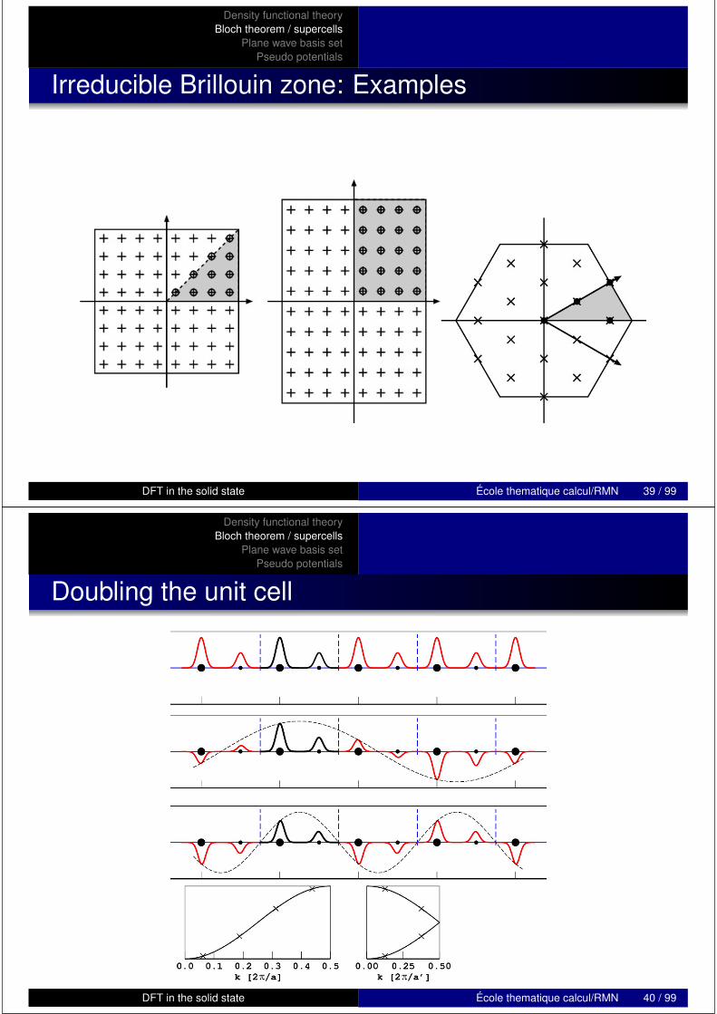
Symmetry operations
If the atoms are related by symmetry operation S(Sψ (r) = ψ (Sr)) the integration over the whole 1stBrillouin zone can be reduced into the irreducible Brillouinzone, IBZ
Sψik (r) = ψik (Sr) = eik·Sruik (Sr) = eik′·ruik′ (r) , k′ = S−1k
∫k
dk ≈∑
k∈BZ
wk =∑
k∈IBZ
∑S
w ′Sk
DFT in the solid state École thematique calcul/RMN 38 / 99
Density functional theoryBloch theorem / supercells
Plane wave basis setPseudo potentials
Irreducible Brillouin zone: Examples
DFT in the solid state École thematique calcul/RMN 39 / 99
Density functional theoryBloch theorem / supercells
Plane wave basis setPseudo potentials
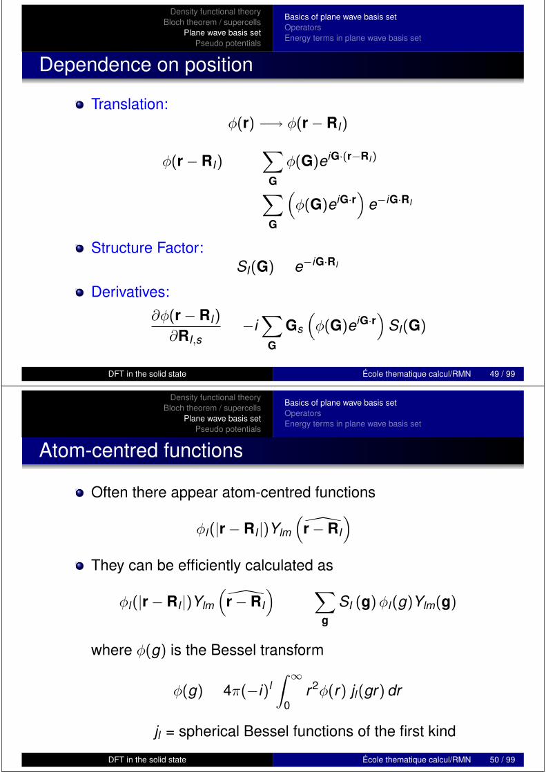
Doubling the unit cell
DFT in the solid state École thematique calcul/RMN 40 / 99

Density functional theoryBloch theorem / supercells
Plane wave basis setPseudo potentials
Doubling the unit cell (super-cells)
If one doubles the unit cell in one direction, it is enough totake only half of the k points in the corresponding directionin the reciprocal spaceAnd has to be careful when comparing energies in cellswith different size unless either equivalent sampling of kpoints is used or one is converged in the total energy inboth cases
DFT in the solid state École thematique calcul/RMN 41 / 99
Density functional theoryBloch theorem / supercells
Plane wave basis setPseudo potentials
Basics of plane wave basis setOperatorsEnergy terms in plane wave basis set
Summary
1 Density functional theory
2 Bloch theorem / supercells
3 Plane wave basis setBasics of plane wave basis setOperatorsEnergy terms in plane wave basis set
4 Pseudo potentials
DFT in the solid state École thematique calcul/RMN 42 / 99

Density functional theoryBloch theorem / supercells
Plane wave basis setPseudo potentials
Basics of plane wave basis setOperatorsEnergy terms in plane wave basis set
Kohn–Sham method
The ground state energy is obtained as the solution of aconstrained minimisation of the Kohn-Sham energy:
minΦ
EKS[Φi(r)]
∫Φ
i (r)Φj(r)dr = δij
DFT in the solid state École thematique calcul/RMN 43 / 99
Density functional theoryBloch theorem / supercells
Plane wave basis setPseudo potentials
Basics of plane wave basis setOperatorsEnergy terms in plane wave basis set
Expansion using a basis set
For practical purposes it is necessary to expand theKohn-Sham orbitals using a set of basis functionsBasis set ϕα(r)M
α=1
Usually a linear expansion
ψi(r) =M∑α=1
cαiϕα(r)
DFT in the solid state École thematique calcul/RMN 44 / 99

Density functional theoryBloch theorem / supercells
Plane wave basis setPseudo potentials
Basics of plane wave basis setOperatorsEnergy terms in plane wave basis set
Plane waves
PhilosophyAssemblies of atoms are slight distortions to free electrons
ϕα(r) =1√Ω
eiGα·r
(. . . = cos(Gα · r) + i sin(Gα · r))+ orthogonal+ independent of atomic positions+ no BSSE± naturally periodic– many functions needed
DFT in the solid state École thematique calcul/RMN 45 / 99
Density functional theoryBloch theorem / supercells
Plane wave basis setPseudo potentials
Basics of plane wave basis setOperatorsEnergy terms in plane wave basis set
Computational box
Box matrix : h = [a1,a2,a3]
Box volume : Ω = det hDFT in the solid state École thematique calcul/RMN 46 / 99

Density functional theoryBloch theorem / supercells
Plane wave basis setPseudo potentials
Basics of plane wave basis setOperatorsEnergy terms in plane wave basis set
Lattice vectors
Direct lattice h = [a1,a2,a3]
Translations in direct lattice: L = i · a1 + j · a2 + k · a3
Reciprocal lattice 2π(ht)−1 = [b1,b2,b3]
bi · aj = 2πδij
Reciprocal lattice vectors : G = i · b1 + j · b2 + k · b3
DFT in the solid state École thematique calcul/RMN 47 / 99
Density functional theoryBloch theorem / supercells
Plane wave basis setPseudo potentials
Basics of plane wave basis setOperatorsEnergy terms in plane wave basis set
Expansion of Kohn-Sham orbitals
Plane wave expansion
ψik(r) =∑
G
cik(G)ei(k+G)·r
To be solved: Coefficients cik(G)
Different routes:Direct optimisation of total energyIterative diagonalisation/minimisation
DFT in the solid state École thematique calcul/RMN 48 / 99
Density functional theoryBloch theorem / supercells
Plane wave basis setPseudo potentials
Basics of plane wave basis setOperatorsEnergy terms in plane wave basis set
Dependence on position
Translation:φ(r) −→ φ(r − RI)
φ(r − RI) =∑
G
φ(G)eiG·(r−RI)
=∑
G
(φ(G)eiG·r
)e−iG·RI
Structure Factor:SI(G) = e−iG·RI
Derivatives:
∂φ(r − RI)
∂RI,s= −i
∑G
Gs
(φ(G)eiG·r
)SI(G)
DFT in the solid state École thematique calcul/RMN 49 / 99
Density functional theoryBloch theorem / supercells
Plane wave basis setPseudo potentials
Basics of plane wave basis setOperatorsEnergy terms in plane wave basis set
Atom-centred functions
Often there appear atom-centred functions
φl(|r − RI |)Ylm
(r − RI
)They can be efficiently calculated as
φl(|r − RI |)Ylm
(r − RI
)=
∑g
SI (g)φl(g)Ylm(g)
where φ(g) is the Bessel transform
φ(g) = 4π(−i)l∫ ∞
0r2φ(r) jl(gr) dr
jl = spherical Bessel functions of the first kind
DFT in the solid state École thematique calcul/RMN 50 / 99

Density functional theoryBloch theorem / supercells
Plane wave basis setPseudo potentials
Basics of plane wave basis setOperatorsEnergy terms in plane wave basis set
Plane waves: Kinetic energy
Kinetic energy operator in the plane wave basis:
−12∇2ϕG(r) = −1
2(iG)2 1√
ΩeiG·r =
12
G2ϕG(r)
Thus the operator is diagonal in the plane wave basis set
Ekin(G) =12
G2
DFT in the solid state École thematique calcul/RMN 51 / 99
Density functional theoryBloch theorem / supercells
Plane wave basis setPseudo potentials
Basics of plane wave basis setOperatorsEnergy terms in plane wave basis set
Cutoff: Finite basis set
Choose all basis functions intothe basis set that fulfill
12
G2 ≤ Ecut
— a cut-off sphere
NPW ≈ 12π2 ΩE3/2
cut [a.u.]
Basis set size depends on volume of box and cutoff only— and is variational!
DFT in the solid state École thematique calcul/RMN 52 / 99

Density functional theoryBloch theorem / supercells
Plane wave basis setPseudo potentials
Basics of plane wave basis setOperatorsEnergy terms in plane wave basis set
Plane waves: Fast Fourier Transform
The information contained in ψ(G) and ψ(r) are equivalent
ψ(G) ←→ ψ(r)
Transform from ψ(G) to ψ(r) and back is done using fastFourier transforms (FFT’s)Along one direction the number of operations ∝ N log[N]
3D-transform = three subsequent 1D-transformsInformation can be handled always in the most appropriatespace
DFT in the solid state École thematique calcul/RMN 53 / 99
Density functional theoryBloch theorem / supercells
Plane wave basis setPseudo potentials
Basics of plane wave basis setOperatorsEnergy terms in plane wave basis set
Plane waves: Integrals
Parseval’s theorem
Ω∑
G
A(G)B(G) =Ω
N
∑i
A(ri)B(ri)
Proof.
I =
∫Ω
A(r)B(r)dr
=∑GG′
A(G)B(G)
∫exp[−iG · r] exp[iG′ · r]dr
=∑GG′
A(G)B(G) Ω δGG′ = Ω∑
G
A(G)B(G)
DFT in the solid state École thematique calcul/RMN 54 / 99

Density functional theoryBloch theorem / supercells
Plane wave basis setPseudo potentials
Basics of plane wave basis setOperatorsEnergy terms in plane wave basis set
Plane waves: Electron density
n(r) =∑
ik
wkfik|ψik(r)|2 =1Ω
∑ik
wkfik∑G,G′
cik(G)cik(G′)ei(G−G′)·r
n(r) =2Gmax∑
G=−2Gmax
n(G)eiG·r
The electron density can be expanded exactly in a plane wavebasis with a cut-off four times the basis set cutoff.
NPW(4Ecut) = 8NPW(Ecut)
DFT in the solid state École thematique calcul/RMN 55 / 99
Density functional theoryBloch theorem / supercells
Plane wave basis setPseudo potentials
Basics of plane wave basis setOperatorsEnergy terms in plane wave basis set
Plane waves: Operators
The Kohn-Sham equations written in reciprocal space:−1
2∇2 + VKS(G,G′)
ψik (G) = εiψik (G)
However, it is better to do it like Car and Parrinello (1985)suggested: Always use the appropriate space (via FFT)There one needs to apply an operator on a wave function:∑
G′O(G,G′)ψ
(G′) =
∑G′
c(G′) 〈G|O|G′〉
Matrix representation of operators in: O(G,G′) = 〈G|O|G′〉Eg. Kinetic energy operator
TG,G′ = 〈G| − 12∇2|G′〉 =
12
G2δG,G′
DFT in the solid state École thematique calcul/RMN 56 / 99

Density functional theoryBloch theorem / supercells
Plane wave basis setPseudo potentials
Basics of plane wave basis setOperatorsEnergy terms in plane wave basis set
Plane waves: Local operators
〈G′|O(r)|G”〉 =1Ω
∑G
O(G)
∫e−iG′·reiG·reiG”·rdr
=1Ω
∑G
O(G)
∫ei(G−G′+G”)·rdr
=1Ω
O(G′ − G”)
Local operators can be expanded in plane waves with a cutofffour times the basis set cutoff
DFT in the solid state École thematique calcul/RMN 57 / 99
Density functional theoryBloch theorem / supercells
Plane wave basis setPseudo potentials
Basics of plane wave basis setOperatorsEnergy terms in plane wave basis set
Plane waves: Applying operators
B(G) =∑G′
O(G,G′)A(G′)
Local operators: Convolution
B(G) =∑G′
1Ω
O(G − G′)A(G′) = (O ∗ A)(G)
Convolution in frequency space transforms to product inreal space:
B(ri) = O(ri)A(ri)
DFT in the solid state École thematique calcul/RMN 58 / 99

Density functional theoryBloch theorem / supercells
Plane wave basis setPseudo potentials
Basics of plane wave basis setOperatorsEnergy terms in plane wave basis set
Kohn–Sham energy
EKS = Ekin + EES + Epp + Exc
Ekin Kinetic energyEES Electrostatic energy (sum of electron-electron
interaction + nuclear core-electron interaction +ion-ion interaction)
Epp Pseudo potential energy not included in EES
Exc Exchange–correlation energy
DFT in the solid state École thematique calcul/RMN 59 / 99
Density functional theoryBloch theorem / supercells
Plane wave basis setPseudo potentials
Basics of plane wave basis setOperatorsEnergy terms in plane wave basis set
Kinetic energy
Ekin =∑
ik
wkfik〈ψik|−12∇2|ψik〉
=∑
ik
wkfik∑GG′
c∗ik(G)cik(G′)〈k + G|−1
2∇2|k + G′〉
=∑
ik
wkfik∑GG′
c∗ik(G)cik(G′) Ω
12|k + G|2 δG,G′
= Ω∑
ik
wkfik∑
G
12|k + G|2 |cik(G)|2
DFT in the solid state École thematique calcul/RMN 60 / 99

Density functional theoryBloch theorem / supercells
Plane wave basis setPseudo potentials
Basics of plane wave basis setOperatorsEnergy terms in plane wave basis set
Periodic Systems
Hartree-like terms are most efficiently evaluated inreciprocal space via the
Poisson equation
∇2VH(r) = −4πntot(r)
VH(G) = 4πn(G)
G2
VH(G) is a local operator with same cutoff as ntot
DFT in the solid state École thematique calcul/RMN 61 / 99
Density functional theoryBloch theorem / supercells
Plane wave basis setPseudo potentials
Basics of plane wave basis setOperatorsEnergy terms in plane wave basis set
Electrostatic energy
EES =12
∫∫n(r)n(r′)|r − r′| dr′dr+
∑I
∫n(r)V I
core(r)dr+12
∑I =J
ZIZJ
|RI − rJ |
The isolated terms do not converge; the sum only forneutral systemsGaussian charge distributions a’la Ewald summation:
nIc(r) = − ZI(
RcI
)3π−3/2 exp
[−
(r − RI
RcI
)2]
Electrostatic potential due to nIc:
V Icore(r) =
∫nI
c(r′)|r − r′|dr′ = − ZI
|r − RI |erf[ |r − RI |
RcI
]DFT in the solid state École thematique calcul/RMN 62 / 99

Density functional theoryBloch theorem / supercells
Plane wave basis setPseudo potentials
Basics of plane wave basis setOperatorsEnergy terms in plane wave basis set
Electrostatic energy
EES =12
∫ ∫dr dr′
n(r)n(r′)|r − r′| +
12
∫ ∫dr dr′
nc(r)nc(r′)|r − r′|
+
∫ ∫dr dr′
nc(r)n(r′)|r − r′|
+12
∑I =J
ZIZJ
|RI − rJ |−12
∫ ∫dr dr′
nc(r)nc(r′)|r − r′|
where nc(r) =∑
I nIc(r)
The first three terms can be combined to the electrostaticenergy of a total charge distribution
ntot(r) = n(r) + nc(r)
and the other two terms calculated analytically.DFT in the solid state École thematique calcul/RMN 63 / 99
Density functional theoryBloch theorem / supercells
Plane wave basis setPseudo potentials
Basics of plane wave basis setOperatorsEnergy terms in plane wave basis set
Electrostatic energy
EES =12
∫ ∫dr dr′
ntot(r)ntot(r′)|r − r′|
+12
∑I =J
ZIZJ
|RI − rJ |erfc
⎡⎣ |RI − rJ |√
RcI2 + Rc
J2
⎤⎦
−∑
I
1√2π
Z 2I
RcI
1. Term: Long-ranged forces; reciprocal space2. Term: Short-ranged two-center terms; real space3. Term: One-center term
DFT in the solid state École thematique calcul/RMN 64 / 99

Density functional theoryBloch theorem / supercells
Plane wave basis setPseudo potentials
Basics of plane wave basis setOperatorsEnergy terms in plane wave basis set
Electrostatic energy: Long-ranged forces
Plane wave expansion of ntot
ntot(G) = n(G) +∑
I
nIc(G)SI(G)
= n(G) − 1Ω
∑I
ZI√4π
exp[−1
2G2Rc
I2]
SI(G)
Criterion for parameter RcI : PW expansion of nI
c has to beconverged with density cut-off
Poisson equation
VH(G) = 4πntot(G)
G2
DFT in the solid state École thematique calcul/RMN 65 / 99
Density functional theoryBloch theorem / supercells
Plane wave basis setPseudo potentials
Basics of plane wave basis setOperatorsEnergy terms in plane wave basis set
Electrostatic energy
Electrostatic energy
EES = 2πΩ∑G=0
|ntot(G)|2G2 + Eovrl − Eself
Eovrl =∑′
I,J
∑L
ZIZJ
|RI − rJ − L|erfc
⎡⎣ |RI − rJ − L|√
RcI2 + Rc
J2
⎤⎦
Eself =∑
I
1√2π
Z 2I
RcI
Sums expand over all atoms in the simulation cell, all directlattice vectors L; the prime in the first sum indicates thatI < J is imposed for L = 0.
DFT in the solid state École thematique calcul/RMN 66 / 99
Density functional theoryBloch theorem / supercells
Plane wave basis setPseudo potentials
Basics of plane wave basis setOperatorsEnergy terms in plane wave basis set
Exchange-correlation energy
Exc =
∫rn(r)εxc(r)dr = Ω
∑G
εxc(G)n(G)
εxc(G) is not local in G space; the calculation in real spacerequires very accurate integration scheme.If the function εxc(r) requires the gradients of the density,they are calculated using reciprocal space, otherwise thecalculation is done in real space (for LDA and GGA; hybridfunctionals are more intensive)
DFT in the solid state École thematique calcul/RMN 67 / 99
Density functional theoryBloch theorem / supercells
Plane wave basis setPseudo potentials
Basics of plane wave basis setOperatorsEnergy terms in plane wave basis set
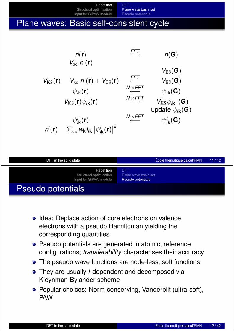
Plane waves: Basic self-consistent cycle
n(r) FFT−→ n(G)Vxc[n](r)
VES(G)
VKS(r) = Vxc[n](r) + VES(r) FFT←− VES(G)
ψik(r) Ni×FFT←− ψik(G)
VKS(r)ψik(r) Ni×FFT−→ [VKSψik] (G)update ψik(G)
ψ′ik(r) Ni×FFT←− ψ′
ik(G)
n′(r) =∑
ik wkfik∣∣ψ′
ik(r)∣∣2
DFT in the solid state École thematique calcul/RMN 68 / 99

Density functional theoryBloch theorem / supercells
Plane wave basis setPseudo potentials
Basics of plane wave basis setOperatorsEnergy terms in plane wave basis set
Plane waves: Calculation of forces
With the plane wave basis set one can apply the
Hellmann-Feynman theorem
(FI =) − ddRI
〈Ψ | HKS | Ψ〉 = −〈Ψ | ∂
∂RIHKS | Ψ〉
All the terms where RI appear explicitly are in reciprocalspace, and are thus very simple to evaluate:
∂
∂RIe−iG·RI = −iGe−iG·RI
DFT in the solid state École thematique calcul/RMN 69 / 99
Density functional theoryBloch theorem / supercells
Plane wave basis setPseudo potentials
Basics of plane wave basis setOperatorsEnergy terms in plane wave basis set
Plane waves: Summary
Plane waves are delocalised, periodic basis functionsPlenty of them are needed, however the operations aresimpleThe quality of basis set adjusted using a single parametre,the cut-off energyFast Fourier-transform used to efficiently switch betweenreal and reciprocal spaceForces and Hartree term/Poisson equation are trivialThe system has to be neutral ! Usual approach for chargedstates: Homogeneous neutralising backgroundThe energies must only be compared with the same Ecut
DFT in the solid state École thematique calcul/RMN 70 / 99

Density functional theoryBloch theorem / supercells
Plane wave basis setPseudo potentials
Introduction to pseudo potentialsGeneration of pseudo potentials
Summary
1 Density functional theory
2 Bloch theorem / supercells
3 Plane wave basis set
4 Pseudo potentialsIntroduction to pseudo potentialsGeneration of pseudo potentials
DFT in the solid state École thematique calcul/RMN 71 / 99
Density functional theoryBloch theorem / supercells
Plane wave basis setPseudo potentials
Introduction to pseudo potentialsGeneration of pseudo potentials
Why use pseudo potentials?
Reduction of basis set sizeeffective speedup of calculationReduction of number of electronsreduces the number of degrees of freedomFor example in Pt: 10 instead of 78Unnecessary “Why bother? They are inert anyway...”Inclusion of relativistic effectsrelativistic effects can be included "partially" into effectivepotentials
DFT in the solid state École thematique calcul/RMN 72 / 99

Density functional theoryBloch theorem / supercells
Plane wave basis setPseudo potentials
Introduction to pseudo potentialsGeneration of pseudo potentials
Why pp? Estimate for number of plane waves
plane wave cutoff ↔ most localized function
1s Slater type function ≈ exp[−Zr ]Z: effective nuclear charge
φ1s(G) ≈ 16πZ 5/2
G2 + Z 2
Cutoff Plane wavesH 1 1Li 4 8C 9 27Si 27 140Ge 76 663
DFT in the solid state École thematique calcul/RMN 73 / 99
Density functional theoryBloch theorem / supercells
Plane wave basis setPseudo potentials
Introduction to pseudo potentialsGeneration of pseudo potentials
Pseudo potential
What is it?
Replacement of the all-electron, −Z/r problem with aHamiltonian containing an effective potentialIt should reproduce the necessary physical properties ofthe full problem at the reference stateThe potential should be transferable, ie. also be accuratein different environments
The construction consists of two steps of approximationsFrozen core approximationPseudisation
DFT in the solid state École thematique calcul/RMN 74 / 99

Density functional theoryBloch theorem / supercells
Plane wave basis setPseudo potentials
Introduction to pseudo potentialsGeneration of pseudo potentials
Frozen core approximation
Core electrons are chemically inertCore/valence separation is sometimes not clearCore wavefunctions are from atomic reference calculationCore electrons of different atoms do not overlap
DFT in the solid state École thematique calcul/RMN 75 / 99
Density functional theoryBloch theorem / supercells
Plane wave basis setPseudo potentials
Introduction to pseudo potentialsGeneration of pseudo potentials
Remaining problems
Valence wavefunctions must be orthogonal to core states→ nodal structures → high plane wave cutoffThus pseudo potential should produce node-less functionsand include Pauli repulsionPseudo potential replaces Hartree and XC potential due tothe core electronsXC functionals are not linear: approximation
EXC(nc + nv) = EXC(nc) + EXC(nv)
This assumes that core and valence electrons do notoverlap. This restriction can be overcome with the"non–linear core correction" (NLCC) discussed later
DFT in the solid state École thematique calcul/RMN 76 / 99

Density functional theoryBloch theorem / supercells
Plane wave basis setPseudo potentials
Introduction to pseudo potentialsGeneration of pseudo potentials
Atomic pseudo potentials: Basic idea
1 Create a pseudo potential for each atomic speciesseparately, in a reference state (usually a neutral or slightlyionised atom)
2 Use these in the Kohn-Sham equations for the valenceonly
(T + V (r, r′) + VH(nv) + VXC(nv)
)Φv
i (r) = εiΦvi (r)
GoalPseudo potential V (r, r′) has to be chosen such that the mainproperties of the all-electron atom are imitated as well aspossible
DFT in the solid state École thematique calcul/RMN 77 / 99
Density functional theoryBloch theorem / supercells
Plane wave basis setPseudo potentials
Introduction to pseudo potentialsGeneration of pseudo potentials
Pseudisation of valence wave functions
DFT in the solid state École thematique calcul/RMN 78 / 99

Density functional theoryBloch theorem / supercells
Plane wave basis setPseudo potentials
Introduction to pseudo potentialsGeneration of pseudo potentials
Generation of pseudo potentials: General recipe
1 Atomic all–electron calculation (reference state)⇒ Φv
l (r) and εl .2 Pseudize Φv
l ⇒ ΦPSl
3 Calculate potential from
[T + Vl(r)] ΦPSl (r) = εlΦ
PSl (r)
4 Calculate pseudo potential by unscreening of Vl(r)
V PSl (r) = Vl(r) − VH(nPS) − VXC(nPS)V PS
l is dependent on l ! Otherwise poor transferability
DFT in the solid state École thematique calcul/RMN 79 / 99
Density functional theoryBloch theorem / supercells
Plane wave basis setPseudo potentials
Introduction to pseudo potentialsGeneration of pseudo potentials
Semi-local pseudo potential
Semi-local form
V PS(r, r′) =∑
l
V PSl (r) | Ylm(r)〉〈Ylm(r′) |
where Ylm are spherical harmonics
This form leads, however, to large computing requirements inplane wave basis sets
DFT in the solid state École thematique calcul/RMN 80 / 99

Density functional theoryBloch theorem / supercells
Plane wave basis setPseudo potentials
Introduction to pseudo potentialsGeneration of pseudo potentials
Norm-conserving pseudo potentials
Hamann-Schlüter-Chiang-Recipe (HSC) conditionsD R Hamann, M Schlüter & C Chiang, Phys Rev Lett 43, 1494 (1979)
1 Real and pseudo valence eigenvalues agree for a chosenprototype atomic configuration: εl = εl
2 Real and pseudo atomic wave functions agree beyond achosen core radius rc : Ψl(r) = Φl(r) for r ≥ rc
3 Integral from 0 to R of the real and pseudo chargedensities agree for R ≥ rc (norm conservation):〈Φl |Φl〉R = 〈Ψl |Ψl〉R for R ≥ rc , 〈Φ|Φ〉R =
∫ R0 r2|φ(r)|2dr
4 The logarithmic derivatives of the real and pseudo wavefunction and their first energy derivatives agree for r ≥ rc .
Points 3) and 4) are related via−1
2
[(rΦ)2 d
dεddr lnΦ
]R =
∫ R0 r2|Φ|2dr
DFT in the solid state École thematique calcul/RMN 81 / 99
Density functional theoryBloch theorem / supercells
Plane wave basis setPseudo potentials
Introduction to pseudo potentialsGeneration of pseudo potentials
Recipes for norm-conserving pseudo potentials
Bachelet-Hamann-Schüter (BHS) form
G B Bachelet et al., Phys Rev B 26, 4199 (1982)
Recipe and analytic form of V PSl
Kerker recipe G P Kerker, J Phys C 13, L189 (1980)
analytic pseudisation functionD. Vanderbilt, Phys Rev B 32, 8412 (1985)
Kinetic energy optimized pseudo potentials
A M Rappe et al., Phys Rev B 41, 1227 (1990)J S Lin et al., Phys Rev B 47, 4174 (1993)
DFT in the solid state École thematique calcul/RMN 82 / 99

Density functional theoryBloch theorem / supercells
Plane wave basis setPseudo potentials
Introduction to pseudo potentialsGeneration of pseudo potentials
Troullier–Martins recipe
N Troullier and J L Martins, Phys Rev B 43, 1993 (1991)
ΦPSl (r) = r l+1ep(r) r ≤ rc
p(r) = c0 + c2r2 + c4r4 + c6r6 + c8r8 + c10r10 + c12r12
determine cn fromnorm–conservationsmoothness at rc (for m = 0 . . .4)dmΦdrm
∣∣∣r=rc−
= dmΦdrm
∣∣∣r=rc+
dΦdr
∣∣r=0 = 0
DFT in the solid state École thematique calcul/RMN 83 / 99
Density functional theoryBloch theorem / supercells
Plane wave basis setPseudo potentials
Introduction to pseudo potentialsGeneration of pseudo potentials
Separation of local and nonlocal parts
V PS(r, r′) =∞∑
L=0
V PSL (r)|YL〉〈YL|
Approximation: All potentials with L > Lmax are equal to V PSloc
V PS(r, r′) =Lmax∑L=0
V PSL (r)|YL〉〈YL| +
∞∑L=Lmax+1
V PSloc(r)|YL〉〈YL|
=Lmax∑L=0
(V PS
L (r) − V PSloc(r)
) |YL〉〈YL| +∞∑
L=0
V PSloc(r)|YL〉〈YL|
=Lmax∑L=0
(V PS
L (r) − V PSloc(r)
) |YL〉〈YL| + V PSloc(r)
DFT in the solid state École thematique calcul/RMN 84 / 99

Density functional theoryBloch theorem / supercells
Plane wave basis setPseudo potentials
Introduction to pseudo potentialsGeneration of pseudo potentials
Semi-local pseudo potential
Final semi-local form
V PS(r, r′) = V PSloc(r) +
Lmax∑L=0
∆V PSL (r)|YL〉〈YL|
Local pseudo potential V PSloc
Non-local pseudo potential ∆V PSL = V PS
L − V PSloc
Any L quantum number can have a non-local part
DFT in the solid state École thematique calcul/RMN 85 / 99
Density functional theoryBloch theorem / supercells
Plane wave basis setPseudo potentials
Introduction to pseudo potentialsGeneration of pseudo potentials
DFT in the solid state École thematique calcul/RMN 86 / 99

Density functional theoryBloch theorem / supercells
Plane wave basis setPseudo potentials
Introduction to pseudo potentialsGeneration of pseudo potentials
DFT in the solid state École thematique calcul/RMN 87 / 99
Density functional theoryBloch theorem / supercells
Plane wave basis setPseudo potentials
Introduction to pseudo potentialsGeneration of pseudo potentials
DFT in the solid state École thematique calcul/RMN 88 / 99

Density functional theoryBloch theorem / supercells
Plane wave basis setPseudo potentials
Introduction to pseudo potentialsGeneration of pseudo potentials
Kleinman–Bylander form
Write the pseudo potential terms as
Kleinman-Bylander operator
V KBPS,nl
(r, r′
)=
∑L
|∆VLφL〉ωL〈∆VLφL|
ωL = 〈φL | ∆VL | φL〉
φL is the pseudo wave function
EPS,nl =∑
ik
wkfik∑
L
〈ψik | ∆VLφL〉ωL〈∆VLφL | ψik〉
Now the expression is fully non-local f (r′) f (r) and thuscomputationally efficient also in plane wave basis set!
DFT in the solid state École thematique calcul/RMN 89 / 99
Density functional theoryBloch theorem / supercells
Plane wave basis setPseudo potentials
Introduction to pseudo potentialsGeneration of pseudo potentials
Ghost states
Problem: In Kleinman–Bylander form, the node-less wavefunction is no longer the solution with the lowestenergy
Solution: Carefully tune the local part of the pseudopotential until the ghost states disappear
How to detect ghost states: Look for following propertiesDeviations of the logarithmic derivatives of theenergy of the KB–pseudo potential from thoseof the respective semi-local pseudo potentialor all–electron potential.Comparison of the atomic bound state spectrafor the semi-local and KB–pseudo potentials.Ghost states below the valence states areidentified by a rigorous criteria by Gonze et al
DFT in the solid state École thematique calcul/RMN 90 / 99

Density functional theoryBloch theorem / supercells
Plane wave basis setPseudo potentials
Introduction to pseudo potentialsGeneration of pseudo potentials
Ultra–soft pseudo potentials and PAW method
Many elements require high cutoff for plane wavecalculations
First row elements: O, FTransition metals: Cu, Znf elements: Ce
relax norm-conservation condition∫nPS(r)dr +
∫Q(r)dr = 1
DFT in the solid state École thematique calcul/RMN 91 / 99
Density functional theoryBloch theorem / supercells
Plane wave basis setPseudo potentials
Introduction to pseudo potentialsGeneration of pseudo potentials
Ultra–soft pseudo potentials and PAW method
Augmentation functions Q(r) depend on environment.No full un-screening possible, Q(r) has to be recalculatedfor each atom and atomic position.Complicated orthogonalisation and force calculations.Allows for larger rc , reduces cutoff for all elements to about30 Ry
DFT in the solid state École thematique calcul/RMN 92 / 99
Density functional theoryBloch theorem / supercells
Plane wave basis setPseudo potentials
Introduction to pseudo potentialsGeneration of pseudo potentials
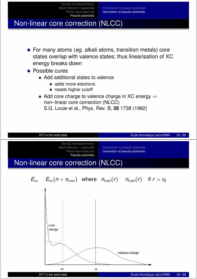
Non-linear core correction (NLCC)
For many atoms (eg. alkali atoms, transition metals) corestates overlap with valence states; thus linearisation of XCenergy breaks downPossible cures
Add additional states to valenceadds more electronsneeds higher cutoff
Add core charge to valence charge in XC energy ⇒non–linear core correction (NLCC)S.G. Louie et al., Phys. Rev. B, 26 1738 (1982)
DFT in the solid state École thematique calcul/RMN 93 / 99
Density functional theoryBloch theorem / supercells
Plane wave basis setPseudo potentials
Introduction to pseudo potentialsGeneration of pseudo potentials
Non-linear core correction (NLCC)
Exc = Exc(n + ncore) where ncore(r) = ncore(r) if r > r0
DFT in the solid state École thematique calcul/RMN 94 / 99

Density functional theoryBloch theorem / supercells
Plane wave basis setPseudo potentials
Introduction to pseudo potentialsGeneration of pseudo potentials
Non-linear core correction (NLCC)
The total core charge of the system depends on the atomicpositions.
ncore(G) =∑
I
nIcore(G)SI(G)
This leads to additional terms in the derivatives wrt to nuclearpositions and the box matrix (for the pressure).
∂Exc
∂RI,s= −Ω
∑G
iGsV xc(G)nI
core(G)SI(G)
DFT in the solid state École thematique calcul/RMN 95 / 99
Density functional theoryBloch theorem / supercells
Plane wave basis setPseudo potentials
Introduction to pseudo potentialsGeneration of pseudo potentials
Specification of pseudo potentials
The pseudo potential recipe used and for each l value rcand the atomic reference stateThe definition of the local potential and which angularmomentum state have a non–local partFor Gauss–Hermit integration: the number of integrationpointsWas the Kleinman–Bylander scheme used ?NLCC: definition of smooth core charge and rloc
DFT in the solid state École thematique calcul/RMN 96 / 99

Density functional theoryBloch theorem / supercells
Plane wave basis setPseudo potentials
Introduction to pseudo potentialsGeneration of pseudo potentials
Testing of pseudo potentials
Calculation of other atomic valence configurations(occupations), comparison with all-electron resultsCalculation of transferability functions, logarithmicderivatives, hardnessCalculation of small molecules, comparison with allelectron calculations (geometry, harmonic frequencies,dipole moments)Calculation of other test systemsCheck of basis set convergence (cutoff requirements)
DFT in the solid state École thematique calcul/RMN 97 / 99
Density functional theoryBloch theorem / supercells
Plane wave basis setPseudo potentials
Introduction to pseudo potentialsGeneration of pseudo potentials
Convergence test for pseudo potentials in O2
DFT in the solid state École thematique calcul/RMN 98 / 99

Density functional theoryBloch theorem / supercells
Plane wave basis setPseudo potentials
Introduction to pseudo potentialsGeneration of pseudo potentials
Pseudo potentials: Summary
Pseudo potential are necessary when using plane wave basissets in order to keep the number of the basis functionmanageable
Pseudo potentials are generated at the reference state;transferability is the quantity describing the accuracy of theproperties at other conditions
The mostly used scheme in plane wave calculations is theTroullier-Martins pseudo potentials in the fully non-local,Kleinman-Bylander form
Once created, a pseudo potential must be tested, tested,tested!!!
DFT in the solid state École thematique calcul/RMN 99 / 99

Plane wave/pseudo potential calculations insolid state — II
Ari P Seitsonen
IMPMC, CNRS & Universités 6 et 7 Paris, IPGP
École thematique calcul/RMN
Different basis setPractical calculations — What to control
Quantum Espresso/PWSCF
Localised basis setsComparison: Localised basis sets vs plane waves
Summary
1 Different basis setLocalised basis setsComparison: Localised basis sets vs plane waves
2 Practical calculations — What to control
3 Quantum Espresso/PWSCF
PWSCF École thematique calcul/RMN 2 / 34

Different basis setPractical calculations — What to control
Quantum Espresso/PWSCF
Localised basis setsComparison: Localised basis sets vs plane waves
Expansion using a basis set
For practical purposes it is necessary to expand theKohn-Sham orbitals using a set of basis functionsBasis set ϕα(r)M
α=1
Usually a linear expansion
ψi(r) =M∑α=1
cαiϕα(r)
PWSCF École thematique calcul/RMN 3 / 34
Different basis setPractical calculations — What to control
Quantum Espresso/PWSCF
Localised basis setsComparison: Localised basis sets vs plane waves
Different basis sets
Plane wavesquantum espresso/PWSCF, CPMD, abinit, paratec, VASP,CASTEP, . . .
Gaussian functionsTurboMole, MolPro, GaussianXX, . . .
Slater functionsADF
Numerical/δ basisDMol3, numol, . . .
MixturesCP2k, Wien2k, . . .
PWSCF École thematique calcul/RMN 4 / 34
Different basis setPractical calculations — What to control
Quantum Espresso/PWSCF
Localised basis setsComparison: Localised basis sets vs plane waves
Atomic orbital basis sets
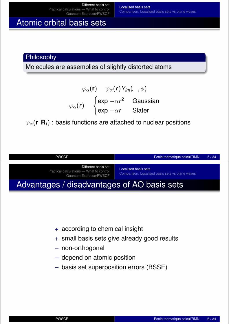
PhilosophyMolecules are assemblies of slightly distorted atoms
ϕα(r) = ϕα(r)Ylm(Θ, φ)
ϕα(r) =
exp[−αr2] Gaussianexp[−αr ] Slater
ϕα(r; RI) : basis functions are attached to nuclear positions
PWSCF École thematique calcul/RMN 5 / 34
Different basis setPractical calculations — What to control
Quantum Espresso/PWSCF
Localised basis setsComparison: Localised basis sets vs plane waves
Advantages / disadvantages of AO basis sets
+ according to chemical insight+ small basis sets give already good results– non-orthogonal– depend on atomic position– basis set superposition errors (BSSE)
PWSCF École thematique calcul/RMN 6 / 34

Different basis setPractical calculations — What to control
Quantum Espresso/PWSCF
Localised basis setsComparison: Localised basis sets vs plane waves
Properties of plane waves
ϕG(r) =1√Ω
exp[iG · r]
Plane waves are periodic wrt. box hPlane waves are orthonormal
〈ϕG′ |ϕG〉 = δG′,G
Plane waves are complete
ψ(r) = ψ(r + L) =1√Ω
∑G
ψ(G) exp[iG · r]
PWSCF École thematique calcul/RMN 7 / 34
Different basis setPractical calculations — What to control
Quantum Espresso/PWSCF
Localised basis setsComparison: Localised basis sets vs plane waves
Comparison to AO basis set
Plane Waves:
12
G2 < Ecut
12
G′2 < Ecut
12
(G + G′)2
<(√
Ecut +√
Ecut
)2= 4Ecut
Atomic orbitals: Every product results in a new function
ϕα(r − A)ϕβ(r − B) = ϕγ(r − C)
Linear dependence for plane waves vs. quadratic dependencefor AO basis sets.
PWSCF École thematique calcul/RMN 8 / 34
Different basis setPractical calculations — What to control
Quantum Espresso/PWSCF
Starting a new calculationUseful toolsExamples of convergence tests
Summary
1 Different basis set
2 Practical calculations — What to controlStarting a new calculationUseful toolsExamples of convergence tests
3 Quantum Espresso/PWSCF
PWSCF École thematique calcul/RMN 9 / 34
Different basis setPractical calculations — What to control
Quantum Espresso/PWSCF
Starting a new calculationUseful toolsExamples of convergence tests
How to start a new calculation
PWSCF École thematique calcul/RMN 10 / 34
Different basis setPractical calculations — What to control
Quantum Espresso/PWSCF
Starting a new calculationUseful toolsExamples of convergence tests
Initial considerations
What is the best method/code available?(classical/approximate/DFT potential)Size of system? (computational resources available)Static or dynamics calculation?
PWSCF École thematique calcul/RMN 11 / 34
Different basis setPractical calculations — What to control
Quantum Espresso/PWSCF
Starting a new calculationUseful toolsExamples of convergence tests
Procedure for DFT calculations
Choice of the system (number of atoms, unit cell, ...; canbe modified later)Test for static computational parametres
description of nuclei (CPMD: pseudo potentials)basis set (CPMD: cut-off energy only)computational unit cell for isolated systems (molecules)exchange-correlation functional
PWSCF École thematique calcul/RMN 12 / 34

Different basis setPractical calculations — What to control
Quantum Espresso/PWSCF
Starting a new calculationUseful toolsExamples of convergence tests
Choice for computational parametres: Unit cell
In plane wave calculations one always has to define acomputational unit cell, even for isolated objects such asatoms or molecules
It should be large enough so that the electronic wavefunctions and density vanish at the boundary of the box, orthat the periodic images of the molecule do not interact witheach otherTest simply by increasing the size of the box systematicallyuntil the main parametres of interest (energies, vibrationalfrequencies, Kohn-Sham eigenvalues, . . . ) do not changeanymore
In naturally periodic systems like solids, liquids, slabgeometries (surfaces, 2-dimensional periodicity), polymers(1-dimensional periodicity) one has to test for theconvergence with respect to k point sampling
PWSCF École thematique calcul/RMN 13 / 34
Different basis setPractical calculations — What to control
Quantum Espresso/PWSCF
Starting a new calculationUseful toolsExamples of convergence tests
Choice for computational parametres: XC functional
Does the system size allow for the use of hybridfunctionals?If not, would LDA provide better accuracy than GGA’s?This is normally the case only in solids or other denselypacked materials, for the bulk properties. Also usedsometimes in cases where GGA’s fail qualitatively (egadsorbtion of molecules with phenyl ring on transitionmetal surfaces)If GGA, which one of them? BLYP (and BP86) is favouredby chemists, PBE by physicistsOther functionals: Meta-GGA’s, asymptotically correctedfunctionals, self-interaction corrected functionals, . . .
PWSCF École thematique calcul/RMN 14 / 34
Different basis setPractical calculations — What to control
Quantum Espresso/PWSCF
Starting a new calculationUseful toolsExamples of convergence tests
Choice for static computational parametres: PP
Considerations when selecting a pseudo potentialWhich valence configuration? Semi-core (= state inbetween “clear” core and valence states; normally−20. . .−50 eV below the vacuum level) in core or valence?Do the core and valence electron density over-lapconsiderably? If yes, is NLCC necessary?Type of pseudo potential? Troullier-Martins, Vanderbilt,other norm-conserving one, . . .Kleinman-Bylander scheme or Gauß-Hermite integration?Which lmax, lloc? The former is more an issue of computingtime, the second crucial to avoidCould the core radii be larger (to reduce basisset/computing time)?
PWSCF École thematique calcul/RMN 15 / 34
Different basis setPractical calculations — What to control
Quantum Espresso/PWSCF
Starting a new calculationUseful toolsExamples of convergence tests
Choice for computational parametres: PP testing
Select a (small) representative system, preferably severalof them; for example of different bonding or hybridisationtypes (eg purely covalent C-C, partially ionic/polarisationC-N or C-H, ionic like H-FStart with a large basis set (please see next topic) in orderto be sure of convergenceCompare to all-electron or other, reliable pseudo potentialcalculation employing the same XC functional, if possible;comparisons with experiments have a second priority, dueto the known, systematic errors in the XC functionalsQuantities to compare: Binding energies, bond lengths,angles, vibrational frequencies, . . .The differences to proper all-electron calculations shouldbe of the order of 0.01 Å or less in bond lengths, < 50 meVfor binding energies, vibrational frequencies < 20 cm−1
PWSCF École thematique calcul/RMN 16 / 34

Different basis setPractical calculations — What to control
Quantum Espresso/PWSCF
Starting a new calculationUseful toolsExamples of convergence tests
Choice for computational parametres: PP parametres
If you need to optimise the parametres of the pseudo potentiallike the core radii, NLCC radius etc, you have to change themand re-run these tests; again until the property of interest doesnot change anymore significantly (Please remember: It isalways nicer to be on the safe side. . . )
PWSCF École thematique calcul/RMN 17 / 34
Different basis setPractical calculations — What to control
Quantum Espresso/PWSCF
Starting a new calculationUseful toolsExamples of convergence tests
Choice for computational parametres: Basis set
With plane wave basis set only one parametre: Cut-offenergy Ecut; units Rydberg atomic units (historical /convenience reasons: Ecut [Ha] = 1
2 |Gmax|2 = 12Ecut [Ry] ⇒
|Gmax| [1/Bohr] =√
Ecut [Ry] )You can start from a low value of Ecut for fast convergence,increase it in steps of 5, 10 or 20 Ry until the properties ofinterest converge; please notice that the total energy of thesystemTypical values
2p elements, transition metals, Troullier-Martins pp’s:50-90 Ry3p, 4p elements, alkali metals with NLCC, transition metalsof the 5p row etc, Troullier-Martins pp’s: 20-40 RyVanderbilt pp’s: 20-35 Ry
PWSCF École thematique calcul/RMN 18 / 34

Different basis setPractical calculations — What to control
Quantum Espresso/PWSCF
Starting a new calculationUseful toolsExamples of convergence tests
Useful tools
units command: Conversion between different units:localhost (~) : units2084 units, 71 prefixes, 32 nonlinear units
You have: 32*(15.9994+2*1.0067) atomicmassunit / (9.885 angstrom)^3You want: g cm^-3
* 0.99094647/ 1.0091362
You have:
openbabel converts between different graphics fileformatsxmgrace or gnuplot for 2-dimensional graphicsxcrysden understand input and output of PWSCFgraphics programs for 3-dimensional plots and atomicconfigurations, movies: gOpenMol vmd, xmakemol, . . .
PWSCF École thematique calcul/RMN 20 / 34
Different basis setPractical calculations — What to control
Quantum Espresso/PWSCF
Starting a new calculationUseful toolsExamples of convergence tests
Convergence tests: Cut-off energy
PWSCF École thematique calcul/RMN 21 / 34

Different basis setPractical calculations — What to control
Quantum Espresso/PWSCF
Starting a new calculationUseful toolsExamples of convergence tests
Convergence tests: k point set
PWSCF École thematique calcul/RMN 22 / 34
Different basis setPractical calculations — What to control
Quantum Espresso/PWSCF
Starting a new calculationUseful toolsExamples of convergence tests
Convergence tests: Cut-off energy
PWSCF École thematique calcul/RMN 23 / 34

Different basis setPractical calculations — What to control
Quantum Espresso/PWSCF
Starting a new calculationUseful toolsExamples of convergence tests
Convergence tests: k point set
PWSCF École thematique calcul/RMN 24 / 34
Different basis setPractical calculations — What to control
Quantum Espresso/PWSCF
IntroductionBasic usageExample
Summary
1 Different basis set
2 Practical calculations — What to control
3 Quantum Espresso/PWSCFIntroductionBasic usageExample
PWSCF École thematique calcul/RMN 25 / 34

Different basis setPractical calculations — What to control
Quantum Espresso/PWSCF
IntroductionBasic usageExample
Quantum Espresso http://www.quantum-espresso.org/
PWSCF École thematique calcul/RMN 26 / 34
Different basis setPractical calculations — What to control
Quantum Espresso/PWSCF
IntroductionBasic usageExample
PWSCF http://www.pwscf.org/
PWSCF École thematique calcul/RMN 27 / 34

Different basis setPractical calculations — What to control
Quantum Espresso/PWSCF
IntroductionBasic usageExample
Quantum Espresso
Historically started from “original” Car-Parrinello codeJoined recently from PWSCF, CPV and FPMD
PWSCF École thematique calcul/RMN 28 / 34
Different basis setPractical calculations — What to control
Quantum Espresso/PWSCF
IntroductionBasic usageExample
Running the executable
Machine-dependent!Serial run:./pw.x -input my-input-file > my-output-file &
Parallel run, linuxmpirun -np $NSLOTS ./pw.x -npool 4 -input my-input-file > my-output-file &
Parallel run, LoadLeveler:./pw.x -npool 4 -input my-input-file > my-output-file &
PWSCF École thematique calcul/RMN 30 / 34

Different basis setPractical calculations — What to control
Quantum Espresso/PWSCF
IntroductionBasic usageExample
Example: fcc-Cu&control
calculation=’scf’restart_mode=’from_scratch’,pseudo_dir = ’/home/seitsonen/usr/espresso/PP_LIBRARY/’,wfcdir=’/tmp/’prefix=’fcc-Cu’tstress = .true.tprnfor = .true.
/&system
ibrav = 2, a = 4.00, b = 4.00, c = 4.00,nat= 1, ntyp= 1,nbnd = 9ecutwfc = 140
! ecutrho = 0occupations=’smearing’, smearing=’fermi-dirac’, degauss=.00367490107593722133
/&electrons
diagonalization=’david’conv_thr = 1.0e-9mixing_beta = 0.8
/ATOMIC_SPECIESCu 63.5500 Cu_pbe-20071125.UPFATOMIC_POSITIONS angstromCu 0.0 0.0 0.0K_POINTS (automatic)16 16 16 0 0 0
PWSCF École thematique calcul/RMN 32 / 34
Different basis setPractical calculations — What to control
Quantum Espresso/PWSCF
IntroductionBasic usageExample
Help on input
Input is explained in file Doc/INPUT_*
One can ask for help on the Mailing list
Different values for ’ibrav/celldm’ are explained at the endof Doc/INPUT_PWPlease be aware on units for lattice vectors andcoordinates: Bohr, Ångström, a0, lattice vectors, . . .
PWSCF École thematique calcul/RMN 34 / 34

Density functional theory in the solid state — III
Ari P Seitsonen
IMPMC, CNRS & Universités 6 et 7 Paris, IPGP
École thematique calcul/RMN
RepetitionStructural optimisation
Input for GIPAW module
DFTPlane wave basis setPseudo potentials
Summary
1 RepetitionDFTPlane wave basis setPseudo potentials
2 Structural optimisation
3 Input for GIPAW module
DFT in the solid state École thematique calcul/RMN 2 / 42

RepetitionStructural optimisation
Input for GIPAW module
DFTPlane wave basis setPseudo potentials
Kohn-Sham schemeKohn-Sham equations
−12∇2 + VKS (r)
ψi (r) = εiψi (r)
n (r) =∑
i
fi |ψi (r)|2
VKS (r) = Vext (r) + VH (r) + Vxc (r)
Vxc (r) = δExcδn(r)
Total energy:
Etot[n] =∑
i
−12
fi⟨ψi | ∇2 | ψi
⟩+
∫rn (r) Vext (r) dr
+12
∫r
∫r′
n (r) n (r′)|r − r′| dr′ dr + Exc + Eion−ion
DFT in the solid state École thematique calcul/RMN 3 / 42
RepetitionStructural optimisation
Input for GIPAW module
DFTPlane wave basis setPseudo potentials
Kohn-Sham equations: Notes
−1
2∇2 + VKS (r)
ψi (r) = εiψi (r) ; n (r) =
∑i
fi |ψi (r)|2
Many-body problem casted into a system of single-particle,coupled equationsSelf-consistent solution requiredεi and ψi are in principle only help variables (only εHOMOhas a meaning)The potential VKS is localThe scheme is in principle exact
DFT in the solid state École thematique calcul/RMN 4 / 42

RepetitionStructural optimisation
Input for GIPAW module
DFTPlane wave basis setPseudo potentials
Exchange-correlation functional
The Kohn-Sham scheme is in principle exact — however,the exchange-correlation energy functional is not knownexplicitlyExchange is known exactly, however its evaluation isusually very time-consuming, and often the accuracy is notimproved over simpler approximations (due toerror-cancellations in the latter group)Many exact properties, like high/low-density limits, scalingrules etc are knownFamous approximations:
Local density approximation, LDAGeneralised gradient approximations, GGAHybrid functionals. . .
DFT in the solid state École thematique calcul/RMN 5 / 42
RepetitionStructural optimisation
Input for GIPAW module
DFTPlane wave basis setPseudo potentials
Exchange-correlation functional: Observations
The accuracy can not be systematically improved!van der Waals interactions still a problem (tailoredapproximations in sight)Most widely used parametrisations:
GGAPerdew-Burke-Ernzerhof, PBE (1996); among phycisistsBeck–Lee-Yang-Parr, BLYP (early 1990’s); among chemists
Hybrid functionalsPBE0; among phycisistsB3LYP; among chemists
DFT in the solid state École thematique calcul/RMN 6 / 42

RepetitionStructural optimisation
Input for GIPAW module
DFTPlane wave basis setPseudo potentials
Integration over reciprocal space
Bloch’s Theorem: The summation over infinite number oftranslations becomes an integral over the first Brillouinzone: ∞∑
L
⇒∫
k∈1.BZdk
In practise the integral is replaced by a weighted sum ofdiscrete points: ∫
kdk ≈
∑k
wk
Eg.n (r) =
∑S
∑k∈1. BZ
wk∑
i
fik |ψik (Sr)|2
DFT in the solid state École thematique calcul/RMN 7 / 42
RepetitionStructural optimisation
Input for GIPAW module
DFTPlane wave basis setPseudo potentials
Expansion of Kohn-Sham orbitals
Plane wave expansion
ψik(r) =∑
G
cik(G)ei(k+G)·r
To be solved: Coefficients cik(G)
+ orthogonal+ independent of atomic positions+ no BSSE± naturally periodic– many functions needed
DFT in the solid state École thematique calcul/RMN 8 / 42

RepetitionStructural optimisation
Input for GIPAW module
DFTPlane wave basis setPseudo potentials
AdvantagesTranslations
φ(r − RI) =∑
G
(φ(G)eiG·r
)e−iG·RI
∂φ(r − RI)
∂RI,s= −i
∑G
Gs
(φ(G)eiG·r
)e−iG·RI
Poisson equation
∇2VH(r) = −4πn(r)
VH(G) = 4πn(G)
G2
Diagonal terms
Ekin = Ω∑
ik
wkfik∑
G
12|k + G|2 |cik(G)|2
DFT in the solid state École thematique calcul/RMN 9 / 42
RepetitionStructural optimisation
Input for GIPAW module
DFTPlane wave basis setPseudo potentials
Cutoff: Finite basis set
Choose all basis functions intothe basis set that fulfill
12
G2 ≤ Ecut
— a cut-off sphere
NPW ≈ 12π2 ΩE3/2
cut [a.u.]
Basis set size depends on volume of box and cutoff only— and is variational!
DFT in the solid state École thematique calcul/RMN 10 / 42
RepetitionStructural optimisation
Input for GIPAW module
DFTPlane wave basis setPseudo potentials
Plane waves: Basic self-consistent cycle
n(r) FFT−→ n(G)Vxc[n](r)
VES(G)
VKS(r) = Vxc[n](r) + VES(r) FFT←− VES(G)
ψik(r) Ni×FFT←− ψik(G)
VKS(r)ψik(r) Ni×FFT−→ [VKSψik] (G)update ψik(G)
ψ′ik(r) Ni×FFT←− ψ′
ik(G)
n′(r) =∑
ik wkfik∣∣ψ′
ik(r)∣∣2
DFT in the solid state École thematique calcul/RMN 11 / 42
RepetitionStructural optimisation
Input for GIPAW module
DFTPlane wave basis setPseudo potentials
Pseudo potentials
Idea: Replace action of core electrons on valenceelectrons with a pseudo Hamiltonian yielding thecorresponding quantitiesPseudo potentials are generated in atomic, referenceconfigurations; transferability characterises their accuracyThe pseudo wave functions are node-less, soft functionsThey are usually l-dependent and decomposed viaKleynman-Bylander schemePopular choices: Norm-conserving, Vanderbilt (ultra-soft),PAW
DFT in the solid state École thematique calcul/RMN 12 / 42

RepetitionStructural optimisation
Input for GIPAW module
DFTPlane wave basis setPseudo potentials
Example: Si
DFT in the solid state École thematique calcul/RMN 13 / 42
RepetitionStructural optimisation
Input for GIPAW module
Optimisation of atomic structureOptimisation of crystal lattice
Summary
1 Repetition
2 Structural optimisationOptimisation of atomic structureOptimisation of crystal lattice
3 Input for GIPAW module
DFT in the solid state École thematique calcul/RMN 14 / 42

RepetitionStructural optimisation
Input for GIPAW module
Optimisation of atomic structureOptimisation of crystal lattice
Structural optimisation
In the beginning of the calculation the atomic coordinatesare usually not accurate (= not at equilibrium of the DFTmethod), coming from
ExperimentsClassical simulationsEducated guess (“chemical intuition”)
Task: Optimise the atomic coordinates and maybe thecrystal parametres= Minimise the total energy with respect to ionic positionsOther type of calculations: Ab initio molecular dynamics(finite ionic T)
DFT in the solid state École thematique calcul/RMN 15 / 42
RepetitionStructural optimisation
Input for GIPAW module
Optimisation of atomic structureOptimisation of crystal lattice
Optimisation of atomic geometry
In principle easy: “Only” (3N-6) degrees of freedom (DoF)However, non-linear and coupled dependency on relativepositionsThe optimisation is much easier if one has the gradientsavailable
Forces acting on the ions
FI = −∇Etot = −∂Etot
∂RI
DFT in the solid state École thematique calcul/RMN 16 / 42
RepetitionStructural optimisation
Input for GIPAW module
Optimisation of atomic structureOptimisation of crystal lattice
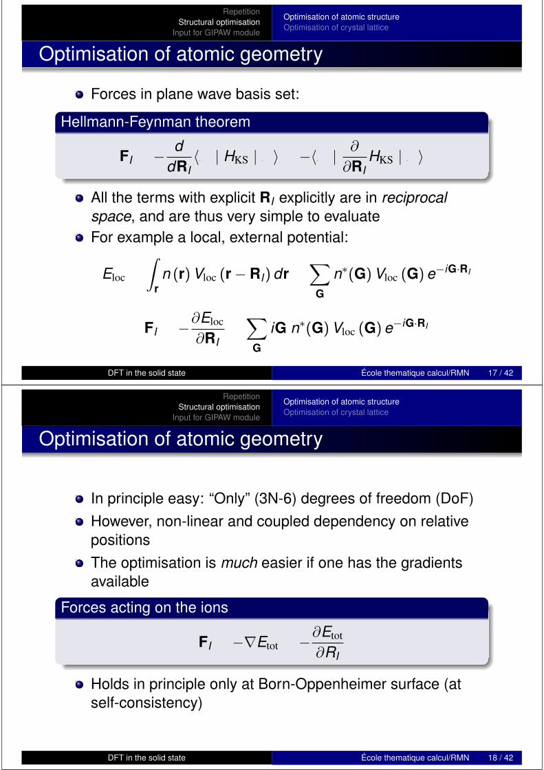
Optimisation of atomic geometry
Forces in plane wave basis set:
Hellmann-Feynman theorem
FI = − ddRI
〈Ψ | HKS | Ψ〉 = −〈Ψ | ∂
∂RIHKS | Ψ〉
All the terms with explicit RI explicitly are in reciprocalspace, and are thus very simple to evaluateFor example a local, external potential:
Eloc =
∫rn (r) Vloc (r − RI) dr =
∑G
n∗(G) Vloc (G) e−iG·RI
FI = −∂Eloc
∂RI=
∑G
iG n∗(G) Vloc (G) e−iG·RI
DFT in the solid state École thematique calcul/RMN 17 / 42
RepetitionStructural optimisation
Input for GIPAW module
Optimisation of atomic structureOptimisation of crystal lattice
Optimisation of atomic geometry
In principle easy: “Only” (3N-6) degrees of freedom (DoF)However, non-linear and coupled dependency on relativepositionsThe optimisation is much easier if one has the gradientsavailable
Forces acting on the ions
FI = −∇Etot = −∂Etot
∂RI
Holds in principle only at Born-Oppenheimer surface (atself-consistency)
DFT in the solid state École thematique calcul/RMN 18 / 42

RepetitionStructural optimisation
Input for GIPAW module
Optimisation of atomic structureOptimisation of crystal lattice
Mathematical formulation
At least close to minimum: Quadratic problem
E = Emin +12
(RI − RminI ) · B · (RI − Rmin
I )
with Hessian BIα,Jβ = ∂2E∂RIα∂RJβ
gradient GIα = ∂E∂RIα
= B · (RI − RminI )
DFT in the solid state École thematique calcul/RMN 19 / 42
RepetitionStructural optimisation
Input for GIPAW module
Optimisation of atomic structureOptimisation of crystal lattice
Optimisation of atomic structure
Newton’s algorithm
Evaluate B and then B−1
Start from a point R(1)I
Calculate gradien G(1)I = GI(R
(1)I )
After movement: R(2) = R(1)I − B−1 · G(1)
I
Since GI(RI) = B · (RI − RminI ), R(2) = Rmin
I
However, evaluation of B would take too long (and system innot harmonic) ⇒ Not a practical schemeQuasi-Newton methods; approximations for B can be used forpre-conditioning
DFT in the solid state École thematique calcul/RMN 20 / 42

RepetitionStructural optimisation
Input for GIPAW module
Optimisation of atomic structureOptimisation of crystal lattice
Optimisation of atomic structure: Algorithms
Steepest descentsConjugate gradientsBroyden-Fletcher-Goldfarb-Shanno (BFGS) methodDamped (Langevin) dynamicsSimulated annealing (molecular dynamics)
DFT in the solid state École thematique calcul/RMN 21 / 42
RepetitionStructural optimisation
Input for GIPAW module
Optimisation of atomic structureOptimisation of crystal lattice
Steepest descents, SD
Steepest descents
At point R(k)I , calculate gradient G(k)
I = GI(R(k)I )
R(k+1)I = R(k)
I − αG(k)I
alpha can be either fixed. . . or searched via line minimisation: Move ions along G(k)
I ,calculate new energy, search for a minimum via harmonicapproximation and move the ions with the final, optimal αCan be very slow eg. in steep valleys
DFT in the solid state École thematique calcul/RMN 22 / 42

RepetitionStructural optimisation
Input for GIPAW module
Optimisation of atomic structureOptimisation of crystal lattice
Direct inversion in iterative sub-space, DIIS
Direct inversion in iterative sub-space, DIIS
Obtain a new point R(k)I = R(k−1)
I − αG(k−1)I , calculate
gradient G(k)I = GI(R
(k)I )
Find GoptI =
∑i≤k αiG
(i)I with
∑α = 1
RoptI =
∑i≤k αiR
(k)I
Update R(k+1)I = Ropt
I − λGoptI
DFT in the solid state École thematique calcul/RMN 23 / 42
RepetitionStructural optimisation
Input for GIPAW module
Optimisation of atomic structureOptimisation of crystal lattice
Broyden-Fletcher-Goldfarb-Shanno, BFGS
Broyden-Fletcher-Goldfarb-Shanno, BFGS
Solve B(k) · s(k) = −G(k)I for s(k)
Perform line search along this direction to obtain α(k)
Obtain the new position from
R(k+1)I = R(k)
I + α(k)s(k)
y(k) =G(k+1)
I − G(k)I
α(k)
B(k+1) = B(k) +y(k) · y(k)
y(k)s(k)− (B(k) · s(k)) · (B(k) · s(k))
s(k) · B(k) · s(k)
DFT in the solid state École thematique calcul/RMN 24 / 42

RepetitionStructural optimisation
Input for GIPAW module
Optimisation of atomic structureOptimisation of crystal lattice
Conjugate gradient, CG
Conjugate gradient, CG
Calculate the gradient at current point, G(k)I = GI(R
(k)I )
Conjugate this gradient as
s(k) = G(k)I + γs(k−1) , γ =
(G(k)I − G(k−1)
I ) · G(k)I
G(k−1)I · G(k)
I
Perform line minimisation along s(k) to obtain R(k+1)I
DFT in the solid state École thematique calcul/RMN 25 / 42
RepetitionStructural optimisation
Input for GIPAW module
Optimisation of atomic structureOptimisation of crystal lattice
Damped dynamics
Damped dynamicsUpdate the positions dynamicallyForces accelerate the ions, velocities are used in a frictionterm to stop them (large forces — fast acceleration, fastmovement — large friction, “cooling”)Equation of motion
R(k)I = −G(k)
I /MI + γs(k−1)
DFT in the solid state École thematique calcul/RMN 26 / 42

RepetitionStructural optimisation
Input for GIPAW module
Optimisation of atomic structureOptimisation of crystal lattice
Quenching dynamics
Quenching/projected dynamicsUpdate the positions dynamicallyForces accelerate the ions, quench if the forces andacceleration are opposite (“overshooting”)Equation of motion
R(k)I = (R(k)
I − R(k−1)I )/(∆t)
V(k)I = R(k)
I · G(k)I
|G(k)I |
G(k)I
|G(k)I |
if R(k)I · G(k)
I < 0, otherwise 0
R(k+1)I = R(k)
I + αV(k)I − (∆t)2G(k)
I
DFT in the solid state École thematique calcul/RMN 27 / 42
RepetitionStructural optimisation
Input for GIPAW module
Optimisation of atomic structureOptimisation of crystal lattice
Simulated annealing
Simulated annealing
Perform molecular dynamics (Newton’s equation ofmotion), reduce the temperature periodicallyAt minimum the forces vanish and the atoms stopIs the “natural” way, however the annealing rates are muchfaster than in eg. in experiments/preparation
DFT in the solid state École thematique calcul/RMN 28 / 42

RepetitionStructural optimisation
Input for GIPAW module
Optimisation of atomic structureOptimisation of crystal lattice
Optimisation of atomic structure
Which algorithm to use?Few degrees of freedom (or robustness required):Conjugate gradientsMedium number of DoF: DIIS, BFGSLarge number of DoF: Damped dynamics or simulatedannealing
DFT in the solid state École thematique calcul/RMN 29 / 42
RepetitionStructural optimisation
Input for GIPAW module
Optimisation of atomic structureOptimisation of crystal lattice
Optimisation of atomic structure
Extrapolation of potential and/or wave function from previousionic steps
Helps to assign a new initial guess for the electronicstructure in the new geometryThus the self-consistent solution is found faster
DFT in the solid state École thematique calcul/RMN 30 / 42

RepetitionStructural optimisation
Input for GIPAW module
Optimisation of atomic structureOptimisation of crystal lattice
Optimisation of crystal structure
It is straightforward to calculate the stress tensor in planewave basis set:
Πuv = − 1Ω
∑s
∂Etot
∂hushT
sv
Eg. kinetic energy
∂Ekin
∂huv= −
∑ik
wkfik∑
G
∑s
GuGs(hT )−1sv |cik (G)|2
Π acts as “gradient” in the update of the lattice vectorsOne has to be careful with discontinuities/jumps in thebasis set when changing the lattice vectors: High accuracyneeded already for stress tensor
DFT in the solid state École thematique calcul/RMN 31 / 42
RepetitionStructural optimisation
Input for GIPAW module
Summary
1 Repetition
2 Structural optimisation
3 Input for GIPAW module
DFT in the solid state École thematique calcul/RMN 32 / 42
RepetitionStructural optimisation
Input for GIPAW module
Parametres affecting scientific output
Exchange-correlation functional (read from pp files)Pseudo potentialsBasis set — Ecut [ecutwfc]k point sampling [section K_POINTS]Convergence: Self-consistency [conv_thr]Spin-polarisation [nspin,multiplicity]Lattice vectors, ionic positions
DFT in the solid state École thematique calcul/RMN 33 / 42
RepetitionStructural optimisation
Input for GIPAW module
Parametres affecting verbosity/control
Algorithm for optimisation of electronic structure[diagonalization]Mixing [mixing_*]Amount of output [verbosity]Restarting [restart_mode]Restarting a parallel calculation [wf_collect]Print-outs [tstress,tprnfor]Organisation of files [outdir,wfcdir]Output filenames [prefix]Computing time [max_seconds]Amount of hard disc/memory [disk_io]Pseudo potentials [pseudo_dir]Symmetries [nosym]
DFT in the solid state École thematique calcul/RMN 34 / 42

RepetitionStructural optimisation
Input for GIPAW module
GIPAW
Chris J Pickard and Francesco Mauri, PRB 63, 245 101 (2001)
Two tasks:1 Gauge-invariance2 Reconstruction of core wave functions
PAW-like transformation
TB = 1+∑I,n
ei/(2c)r·RI×B[∣∣φI,n
⟩ − ∣∣∣φI,n
⟩] ⟨pI,n
∣∣ e−i/(2c)r·RI×B
Slowly-varying field: eiq·x
Macroscopic shape:
B(1)ind (G = 0) =
8π3χB
DFT in the solid state École thematique calcul/RMN 35 / 42
RepetitionStructural optimisation
Input for GIPAW module
GIPAW in PWSCF
First perform a self-consistent run with ’pw.x’Then you can use ’gipaw.x’: The latter uses informationgenerated by ’pw.x’Converge the electronic structure accuratelyThe symmetry operations have to map the coordinate axisinto each other; otherwise the symmetries must beswitched off!
DFT in the solid state École thematique calcul/RMN 36 / 42

RepetitionStructural optimisation
Input for GIPAW module
Example: Hegaxonal lattice, GIPAW-NMR&control
calculation = ’scf’ <<<<<<<<<<<<<<<<<<<<<<<<<<<<! restart_mode = ’from_scratch’
restart_mode = ’restart’prefix = ’b2o3I’tstress = .false.tprnfor = .true.pseudo_dir = ’./’outdir = ’./scratch/’
/&system
ibrav = 4celldm(1) = 8.07450432109878800047celldm(3) = 1.92343173431735265832nat = 15ntyp = 2nspin = 1ecutwfc = 60.0nosym = .true. <<<<<<<<<<<<<<<<<<<<<<<<<<<<
/&electrons
diagonalization = ’cg’mixing_mode = ’plain’mixing_beta = 0.7conv_thr = 1.0d-12 <<<<<<<<<<<<<<<<<<<<<<<<<<<<
/ATOMIC_SPECIESB 10.81 B_pbe-20070929.cpi.UPFO 15.9994 O_pbe-20070929.cpi.UPF
ATOMIC_POSITIONS crystalO 0 555685095948 0 398122479874 -0 003161558426
DFT in the solid state École thematique calcul/RMN 38 / 42
RepetitionStructural optimisation
Input for GIPAW module
Relaxation of ionic positions
&controlcalculation = ’relax’
...etot_conv_thr = 1.0D-7forc_conv_thr = 1.0D-5
.../...&ions
ion_dynamic = ’bfgs’pot_extrapolation = first_orderwfc_extrapolation = first_order
/...
DFT in the solid state École thematique calcul/RMN 40 / 42

RepetitionStructural optimisation
Input for GIPAW module
Relaxation of ionic positions
&inputgipawjob = ’nmr’prefix = ’b2o3I’tmp_dir = ’./scratch/’iverbosity = 1q_gipaw = 0.01read_recon_in_paratec_fmt = .false.file_reconstruction ( 1 ) = "B_AEPS.DAT"file_reconstruction ( 2 ) = "O_AEPS.DAT"use_nmr_macroscopic_shape = .TRUE.
/
DFT in the solid state École thematique calcul/RMN 42 / 42