Department of Electrical and Computer Engineering

EE461: Digital Control - Lab Manual

Winter 2011

EE 461 Experiment #1Digital Control of DC Servomotor

1 Objectives

The objective of this lab is to introduce to the students the design and implementation ofdigital control. The digital control is implemented on a lab-scale DC Servomotor in the con-trol systems laboratory. The performance of the resulted digital control system is comparedwith the continuous-time control system performance. The effect of sampling period Ts (orsampling frequency fs =

1Ts) is studied.

When doing the lab, the software packages MATLAB with Control Systems Toolbox, andthe Simulink are used for the analysis and design of control systems.

2 Introduction

An important approach to digital controller (filter) design is to start with a well-designed ana-log controller. The digital controller C(z) is then implemented by discretizing the continuous-time controller C(s). This design method is also called design by emulation, which iswidely used by control engineers in practice. It is known that for a properly chosen samplingperiod, this method can provide a useful digital controller with satisfactory performance. Inthis lab, students are asked to implement the digital controllers, obtained by discretizinga pre-specified analog controller using some common discretization methods. The effect ofsampling frequency is also studied by comparing different system responses with respect to fs.

In the last part of the experiment, the students are asked to implement a digital controllerdesigned directly for the discrete-time dc-motor model, and the system response is ob-tained for comparison purpose.

1

3 Preparation

Before the lab begins, students are required to read and understand the Control System Lab-oratory Manual for the hardware and software description. In addition, it is recommendedthat the students complete the following pre-lab work.

The Quanser dc-servomotor in the control systems laboratory has the following model (witha low gear ratio and in the load free case): P(s) = 20020

s(s+42). The analog control system can

be implemented by using a continuous-time controller C(s):

Figure 1: Analog Control System for a DC-Motor

In this lab, the analog controller is given as a lead compensator C(s) = 0.08s+0.08s+3

, which cangenerate a satisfactory transient and steady-state performance of the system step response.By discretizing C(s), one can implement a digital control system:

Figure 2: Digital Control System for a DC-Motor

1. With the sampling interval chosen as Ts = 0.001, and Ts = 0.01, use the Bilineartransformation (Tustin’s method) to obtain the discrete-time models of C(s), denotedby C1(z) and C2(z), respectively. This can be done by using c2d command in Matlab.

Record down C(s), C1(z), and C2(z), and they will be used in the following experimentprocedure.

2

4 Experiment Procedure

1. Check and understand the wiring between the dc-motor, power module(UPM) and thecomputer.

2. Start the MATLAB, and Simulink. It can be noticed that a Quanser toolbox is installedin the Simulink, and it contains the blocks to interface with the real system setup.

4.1 Part 1. Implementation of Analog Control

3. Build a simulink model (use Simulink and Quanser toolbox) to implement the analogcontrol system in Figure 1, with C(s) given there. The motor shaft Encoder is used tomeasure the angular position, and a calibration gain of -360/4096 needs to be addedto the encoder to convert the angular signal to ‘degree’. The reference input is set toa step signal of 30 degrees.

4. Compile your program by going to ‘WinCon’ in the manual bar and clicking ‘Build’, aWinCon interface window will then appear if there is no error in your simulink model.Remember to adjust your motor shaft to zero position before start running the systemevery time. You can also select scopes to monitor the signals in real-time. For example,choose scopes to monitor the angular position Θ(t) and the control signal u(t)

5. Run the system by clicking ‘Start’, after 6 seconds (it can be seen from the scope),stop the program by clicking ‘Stop’ and save the data for later analysis. Another wayto stop the program is to add the following timer in your Simulink model, which allowsthe simulation to stop automatically.

Figure 3: Timer

3

4.2 Part 2. Implementation of Digital Control by Emulation

6. Implement the digital control system in Figure 2. Set the sampling time as Ts =0.001 sec., then replace the analog controller in your Simulink model by the discretizedone C1(z). Remember to set the same sampling time in the input block, and in the‘Simulation > Parameters...’ (change simulation method to ‘discrete’, and set the fixedstep size as same as Ts).

7. Repeat steps (4) and (5), and save the data

8. Set Ts = 0.01 sec., implement C2(z). Repeat steps (6) and (7)

4.3 Part 3. Digital Control by Direct Design

In the following steps, we are going to implement a digital controller directly designedbased on the discretized plant (i.e. the ZOH equivalent model of P(s)), rather thandiscretizing an analog controller. This method is referred to as ”direct design method”.

9. By setting Ts = 0.01 sec., a discrete-time compensator of the form C3(z) = K( z−0.657z−0.35

)is chosen. Implement C3(z) in your model, and repeat the steps (4) and (5). Observethe system response and save the data. Note: The gain K in C3(z), can be tuned toget a good performance. ( Warning: the system is very sensitive to the selection ofK, too large K may result in instability, a suitable rang is [0.2, 0.05]), a suitable choiceis K = 0.12)

10. When changing the sampling interval to Ts= 0.1 (a rather slow sampling), one has tore-design the discrete-time compensator, it is chosen as C4(z) = 0.04( z−0.6

z−0.35). Imple-

ment C4(z), and observe the system response.

Caution: during the experiment, the motor may run without control, suchas turning extremely fast and making unpleasant noises, in these cases, stopthe program immediately, and ask for assistance.

5 Analysis and Discussion

Finally, after all the trials, load the data into Matlab and plot the time responses of the dc-motor angular position. Evaluate the performance by calculating the percent of overshoot(P.O.), settling time (Ts, and steady-state error ess. It is recommended to plot the referenceinput signal and the output signals that you want to compare in the same graph.

4

1. Compare the step responses of the dc-motor using the discretized controller C1(z), andC2(z) with that of analog controller C(s), in terms of P.O., Ts, and ess. What can youobserve?

2. How does the sampling time affect the system responses in the experiment in Part 2?

3. Compare the system response by using C3(z) in Part 3, step (9), with the systemresponse using C2(z) in step (8), what can you say about the performance of thesetwo digital controllers? (remember that they are obtained by ”emulation” and ”directdesign”)

4. From all above procedures when trying different sampling intervals, make a discussionon the effects of sampling time to the system performance.

6 Lab Report

Individual reports are required although the students may work in groups. The reportsshould contain:

• The pre-lab work

• A brief introduction of the experiment.

• Printouts of Simulink models, and all the plots.

• Your discussions by answering the question in section 5.

• Any conclusions you would like to draw.

The lab report is due by 4pm on Feb. 14, 2011 for section H3 and 4pm on Feb. 28, 2011 forsection H4. Please drop your report into the box assigned to EE461 LAB outside the mainoffice at 2nd floor ECERF.

5

EE 461 Experiment #2Computer Simulation of Digital Control

Systems

1 Objectives

The objectives of this lab is to perform the inter-sample response analysis and the computersimulation of a sampled-data system using MATLAB.

2 Introduction

A typical sampled-data system is shown in Figure 1, where S and H represent the Sampler(A/D converter) and the Holder (D/A converter) respectively.

Figure 1: Sampled-Data System

Unlike a pure analog system (that has an analog controller and the continuous-time plant), ora pure discrete-time system (with a digital controller and the discretized model of the plant),the sampled-data system has both the digital controller and the continuous-time plant. Thesignals passing through the entire system is a mixture of sampled data and continuous-time signals. Most control system simulation software packages such as MATLAB only havefunctions for continuous-time and discrete-time simulations, e.g., lsim, step, and dstep, dlsim,etc., but none for sampled data simulation. This lab is to write a general MATLAB program(function) to simulate the step response of a sampled-data (digital) control system.

1

3 Preparation

Before the experiment, the students should understand the procedure of the sampled-datasimulation, and the procedure for calculating the inter-sample response.

4 Experiment Procedure

The analog plant P(s) that we considered in this lab is a flexible beam system:

P(s) =1.6188s2 − 0.1575s− 43.9425

s4 + 0.1736s3 + 27.9001s2 + 0.0186s(1)

Assume that you have designed an advanced digital controller for this complex system (atsampling period T = 0.5 sec), i.e. as in Figure 1:

Cd(z) =−0.1084z5 − 0.01202z4 + 0.1708z3 + 0.08469z2 − 0.09198z − 0.04313

z6 − 0.6528z5 − 0.8377z4 + 0.4495z3 + 0.4709z2 − 0.5820z + 0.1521(2)

Before we can implement this digital controller on-line and perform real-time control onthe real flexible beam system, first of all, we need to test the control system performancein a computer environment. This can be achieved by sampled-data (digital) simulation .

The following steps describe the procedure for simulating the step response of the sampled-data system using existing MATLAB functions:

1. Define the models of the digital controller and the analog plant, e.g.

sysC d = tf(numC d, denC d, T) Create a discrete-time transfer function withsampling period T (T = 0.5 )

sysP = tf(numP,denP)

2. Discretize the continuous-time plant P(s) to obtain the ZOH equivalent Pd(z) (Pd(z)= SP(s)H ) via the MATLAB function c2d.

2

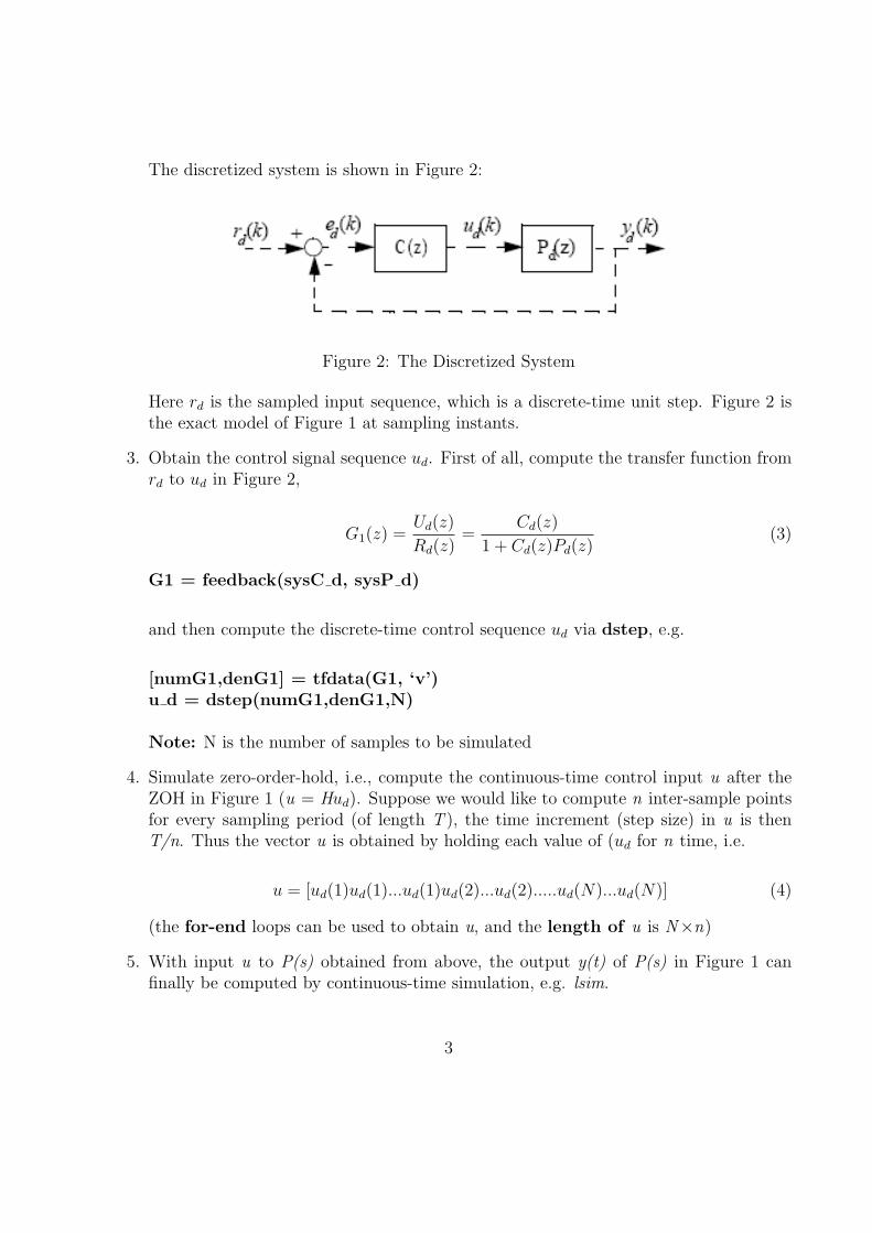
The discretized system is shown in Figure 2:

Figure 2: The Discretized System

Here rd is the sampled input sequence, which is a discrete-time unit step. Figure 2 isthe exact model of Figure 1 at sampling instants.

3. Obtain the control signal sequence ud. First of all, compute the transfer function fromrd to ud in Figure 2,

G1(z) =Ud(z)

Rd(z)=

Cd(z)

1 + Cd(z)Pd(z)(3)

G1 = feedback(sysC d, sysP d)

and then compute the discrete-time control sequence ud via dstep, e.g.

[numG1,denG1] = tfdata(G1, ‘v’)u d = dstep(numG1,denG1,N)

Note: N is the number of samples to be simulated

4. Simulate zero-order-hold, i.e., compute the continuous-time control input u after theZOH in Figure 1 (u = Hud). Suppose we would like to compute n inter-sample pointsfor every sampling period (of length T ), the time increment (step size) in u is thenT/n. Thus the vector u is obtained by holding each value of (ud for n time, i.e.

u = [ud(1)ud(1)...ud(1)ud(2)...ud(2).....ud(N)...ud(N)] (4)

(the for-end loops can be used to obtain u, and the length of u is N×n)

5. With input u to P(s) obtained from above, the output y(t) of P(s) in Figure 1 canfinally be computed by continuous-time simulation, e.g. lsim.

3

(The obtained y(t) is in fact the computer approximation of the actual continuous-timeoutput in the real system. It should be a good approximation because 10 points of theinter-sample response are calculated during each sampling interval T.)

Finally, the above steps can be integrated into a general function named sdstep (orchoose your own preferred name) in MATLAB:

[y,u,t] = sdstep(numC d,denC d,numP,denP,T,N,n)

For this function, the user can define the model of the digital controller in numC d anddenC d, and the model of the continuous-time plant in numP and denP. T and N aresampling period and number of samples to be simulated, respectively; and the integern is the ratio of sampling period T to the time increment T1 used when calculatingthe inter-sample response. The returned variables of the above function are the outputfrom continuous-time plant P(s), y(t) (see Figure 1, and the corresponding input u(t)and the time vector t. (Actually, during debugging and the experiment, you can returnas many inter-variables as you prefer.)

Once you have programmed the function sdstep, perform the following for this exper-iment:

• Debug your program(sdstep.m) and simulate the step responses of the sampled-data system with Cd(z), P(s) given in Eqs. (1) and( 2), with the sampling periodT = 0.5, number of samples N = 40, and the intersample ratio n = 10.

• Calculate the discrete-time output yd based on the control sequence ud and thediscrete-time model using dlsim, the time sequence td can be chosen as

t d = [0:T:(N-1)*T];The time sequence td with N samples and the interval as T

• On the same figure, plot the discrete-time control sequence ud vs. td, and thecontinuous-time control sequence u vs. t, for example, use:

plot(t d,u d,‘*’,t,u,‘r’)

Can you see the effect of the zero-order-hold?

• On the same figure, plot the continuous-time output y vs. t, and the discrete-timeoutput (td vs. yd).

4

plot(t d,y d,‘*’,t,y,‘r’)

Does the discrete-time output samples match the continuous-time output at thesampling instants?

5 Lab Report

Your report should contain:

• A brief introduction.

• Your program in MATLAB for the sampled-data simulation function: sdstep.m

• All the plots.

• Answering the questions given at the end of Section 4.

• Any conclusions you would like to draw.

The lab report is due by 4pm on Mar. 7, 2011 for students in section H3 and 4pm on Mar.14, 2011 for students in section H4. Please drop your report into the box assigned to EE461LAB outside the main office at 2nd floor ECERF.

5

EE 461 Experiment #3

State Feedback Control of the Flexible Link

System

1 Objectives

One of the major advantages of state-space modeling and esign techniques lies in the fact that

they can be easily implemented using computers, which have superior processing power and

speed in handling matrix computations. In this lab, several types of state feedback designs

are implemented on a flexible link setup built by Quanser. The Simulink with Quanser tool

box is used as control system development software. Students are expected to understand the

design procedure of pole placement design technique and some practical issues in applying

theory to real world problems.

2 Introduction

The flexible link apparatus consists of a Quanser DC servomotor - SRV02 and a Flexgage

module mounted on SRV02. For detailed hardware descriptions and the connections, please

refer to the attachment of the Lab Preliminary.

The state space model of the flexible link is given as follows (for more details about the

derivation of this model, see Appendix of flexible link manual, also available at Lab website):

x =

0 0 1 0

0 0 0 1

0 1060.9 −57.658 0

0 −1465.2 57.658 0

x(t) +

0

0

107.39

−107.39

u(t) (1)

1

where x = [θ, α, θ, α]′; θ denotes the motor shaft angle, α the tip deflection angle of the ruler,

θ the motor angle velocity, and α the deflection angle velocity. The input u is the voltage

applied to motor armature.

The design objective for this setup is to move the link within a range of angles (driven by the

motor), while maintaining a small deflection at the tip all the time. This is a typical tracking

plus regulation problem. Two sensors are installed, one is a shaft encoder to measure motor

angle θ, and the other a strain gauge to measure tip deflection angle α. The calibration

factors of the shaft encoder and strain gauge are listed as follows:

• Motor shaft angle: − 2π4096

for radian

• Deflection angle: −0.02540.48

for radian

Since there is no sensor to measure angle velocity, θ and α are estimated by two differential

filters (their functions are to calculate the differentiation of angles), which are implemented

using default Simulink modules.

The following figures illustrate analog and digital state feedback controls. In this lab, we

are going to implement both of them on the flexible link. It needs to be point out that

when implementing digital state feedback control, the selection of sampling period is crucial,

especially for this flexible link, because theoretically it is marginally unstable and also has

under-damped modes that tend to be more oscillatory. This can be observed by checking

the open loop eigenvalues: eig(A). In this case, the analog design can help us to determine

suitable sampling period.

La

(A, B)+_

r(t) u(t) x(t)

(A-BLa, B)r(t) x(t)

Figure 1: Analog state feedback control

2

r(k) x(k)

_ZOH (A, B) S

L

x(t)u(t)u(k)

),( ΓΓ−Φ Lr(k) x(k)

Figure 2: Digital state feedback control

3 Preparation

In the pre-lab section, students are expected to obtain the following results beforehand: 1)

The analog state feedback gain La; 2) The digital state feedback gain L; and 3) A suitable

range of the sampling frequency when implementing the digital state feedback.

Note: It is strongly recommended that you have all the results available at least

before proceeding to the next part of the lab: Implementation. The Lab TA

will check with each group to see whether or not your choice of sampling period

and the computed state feedback gains are correct (or “reasonable”). This is

important, because a “careless” mistake may result in a severe damage on the

hardware. We work with a real system, not a simulation!

1. The set of closed-loop poles for the analog system (in Figure 1) are given as follows:

p = (−150, − 16, − 10 + j15, − 10− j15).

For this set of poles, compute and write down the analog state feedback gain La using

MATLAB functions: place or acker.

2. Once La is obtained, the bandwidth ωB of the analog regulator system can be evaluated

based on the bode plot of the following transfer function. Bode plot can be obtained

using MATLAB function bode( ):

G1(s) = La[sI − (A−BLa)]−1B (2)

The bandwidth is the frequency at which the magnitude response drops 3dB from the

magnitude response at the low frequency, i.e. ω ∼= 0.

The sampling frequency ωs can then be selected within the following ranges: 40 ≤ ωs

ωB≤

3

70. (The upper and lower bound is chosen higher than normally required because of

the open loop characteristics of this flexible link setup: under-damped and marginally

unstable.) Based on the above justification, compute and write down an appropriate

sampling period T = 2πωs.

3. In the following, you are required to compute the digital state feedback gain based on

different design methods:

• First of all, compute the ZOH discrete plant (Φ, Γ) using the c2d function, with

the selected sampling period T (T should be within the above range; a default

choice is T = 0.001sec). (Φ, Γ) will be used in the following steps to obtain digital

state feedback gains.

• With your selection of sampling period T, map the closed-loop poles for the analog

control system in (1) to z-plane poles z, using the mapping relationship z = epT ,

where p = (−150,−16,−10 + j15,−10 − j15). Then use ”place()” or ”acker()”

to compute the digital state feedback gain L1 (in Figure 2) which can achieve the

desired z-plane poles pd.

• In this lab, a Digital Linear Quadratic Regulator (DLQR) is to be implemented as

an alternative controller. This design yields a state feedback controller that can

achieve the stabilization (regulation) objective as well as minimizing the following

performance index:

J =∑k

xT [k]Qx[k] + uT [k]Ru[k] (3)

By selecting

Q =

3000 0 0 0

0 10000 0 0

0 0 15 0

0 0 0 5

and R = 10, compute the optimal state feedback gain using Matlab function

dlqr(). Write it down as L2 for later use.

4 Experiment Procedure

Note: during the experiment, allow enough space for flexible link to turn around.

The motor may run extremely fast and make unpleasant noises. In this case,

stop experiment immediately and ask for help.

4

1) Check and understand the wiring between the DC motor, Flexgage module, power

module (UPM) and the computer.

2) Start the MATLAB and Simulink.

Implementation of Analog State Feedback:

3) Build a Simulink model, and implement the analog state feedback control shown in

Figure 1, with the gain La obtained in Section 3 . Pay attention to the calibration

factors. The reference input is set to a step signal of magnitude 10.

4) Compile your Simulink model by going to ‘WinCon’ in the manual bar and clicking

‘Build’, a WinCon interface window will then appear if there is no error in your model.

Remember to adjust the ruler to zero position before start running the system every

time. Select scopes to monitor the signals in real-time. For example, choose scopes to

monitor the angular position θ, α, and the control signal u.

5) Run the system by clicking ‘Start’, after 4-6 seconds (it can be seen from the scope),

stop the program by clicking ‘Stop’ and save the data for later analysis. Another way to

stop the program is to add a timer in your Simulink model (refer to the Lab 1 manual).

Implementation of Digital State Feedback:

6) Set the sampling period as the value selected in the pre-lab section wherever it is needed

in the Simulink model (default choice is T = 0.001sec). Implement the digital state

feedback control u[k] = −L1x[k], where L1 is obtained by matching the continuous

poles used in the analog design. Repeat the steps 4) and 5). Observe the system

response and save the data.

7) With the sampling period fixed as in 6), implement the digital linear quadratic regulator

u[k] = −L2x[k], and repeat steps 4) and 5). Observe system response and save the

data.

5 Analysis and Discussion

Finally, after all the trials, load the data into MATLAB and plot the time responses of the

motor shaft angular position θ and tip deflection angle α. For the above three state feedback

controllers (i.e., the analog La, the digital L1 by matching continuous closed-loop poles, and

5

the optimal DLQR L2), evaluate and compare the performance by calculating the percentage

of overshoot (P.O.) and settling time (Ts).

Note: Since tracking performance is not explicitly considered in the design of state feedback,

the angle position θ is expected to have a tracking error.

6 Lab Report

Individual reports are required although the students are allowed to work in groups. The

report should contain:

• The pre-lab work.

• A brief introduction of the experiment.

• Printouts of Simulink models and all plots.

• Your analysis and discussions in section 5.

• Any conclusions you would like to draw.

The lab report is due by 4pm on Mar. 21, 2011 for students in section H3 and 4pm on Mar.

28, 2011 for students in section H4. Please drop your report into the box assigned to EE461

LAB outside the main office at 2nd floor ECERF.

6

EE 461 Experiment #4Design of Observer-Based State-feedback

Control for a Flexible Link System

1 Objectives

State estimation(observer) schemes are extremely useful in practical systems, especially whensystems states can not be completely measured. The observer-based state feedback control isone of the most important design techniques for modern control systems. In this experiment,students will be given the opportunity to implement such a controller on a lab-scale flexiblelink system, which is claimed as a difficult system to control because of the inherent under-damped (oscillatory) properties of the system. The “real life” example of this setup is theCanada Arm (the large scale long flexible beam robotic manipulator) in the outer space.

2 Introduction

The state space model of the flexible link is obtained as follows:

x(t) =

0 0 1 00 0 0 10 1060.9 −57.658 00 −1465.2 57.658 0

x(t) +

00

107.39−107.39

u(t),

(1)

where x = [θ, α, θ, α]′; θ represents motor shaft angle, α the tip deflection angle of the ruler,

θ motor angle velocity, and α deflection angle velocity. The input u is the voltage appliedto motor armature. The design objective for this setup is to move the link within a rangeof angles (driven by the motor), while maintaining a small deflection at the tip all the time.This is a typical tracking plus regulation problem. Two sensors are installed, one is the shaftencoder to measure the motor angle θ and the other is the strain gauge to measure the tip

1

deflection angle α. The calibration factors of shaft encoder and strain gauge are listed asfollows:

• Motor shaft angle: − 2π4096

for radian

• Deflection angle: −0.02540.48

for radian

Since there is no sensor instrumented in this setup to measure angle velocities, θ and α willbe estimated in this lab by using a full-order observer, together with the estimated anglesθ and α, four system states will all be available for state feedback control. Recall that inthe experiment 3, the angular velocity rates are calculated by taking differentiations of angles.

From Experiment #3, students may have noticed that the sensor of deflection angle α maynot work very well; there may exist an offset/bias in α measured by the strain gauge. Thisbias is caused by an improperly calibrated sensor. Later when comparing the tip angle, theobservation should be made on the oscillation magnitude of α.

Considering that the system is still observable with one measurement θ, we will consider tobuild an observer based on

y(t) =[1 0 0 0

]x(t).

In this set-up, measurement of α is not needed, and only the measurement of θ is used toconstruct an observer for state vector.

The true state feedback control and the observer-based state feedback control are illustratedin Figure 1 and 2.

Figure 1: True state feedback control

2

Figure 2: Observer-based state feedback control

3 Preparation

Note: It is strongly recommended that you have all the results available at leastbefore you proceed to the next part of the lab: Implementation. The Lab TAwill check with each group to see whether or not your computed state feedbackgains and observer gains are correct (or “reasonable”).

In the pre-lab section, students are expected to obtain the following results: 1) digital statefeedback gain L; 2) digital observer gain K.

1. Digital State Feedback Gain L (with sampling period T = 0.001sec)

• As in Experiment #3, given the closed-loop poles of analog state feedback controlsystem p0 = (−100,−16,−10+ j15,−10− j15), obtain the corresponding z-planepoles using the mapping pd0 = ep0T , T = 0.001.

• Compute the ZOH discrete system plant (Φ,Γ) using MATLAB function ‘c2d’,and then compute the digital state feedback gain L to achieve closed-loop polesat pd0.

2. Digital Observer Gain K

Given two sets of poles p1 = (−200,−70,−20+j15,−20−j15) and p2 = (−120,−30,−20+j15,−20 − j15), map them to z-plane poles pd1 and pd2. Then respectively compute

3

the observer gain K1 and K2 to place observer poles with the ZOH discrete plant (Φ,Γ)obtained in Part 3-1.

4 Experimental Procedure

During the experiment, allow enough space for the flexible link to turn around.The motor may run without control, turning fast and making unpleasant noises.In this case, stop the program immediately, and ask for assistance.

In the following procedures, students are expected to implement both the true state feedbackwith the state feedback gain L obtained in (1) (follow the same procedure as in Experiment#3), and the observer based state feedback control. The responses of the system output θand α, are compared in these two designs. Estimation error of the observer will be examined.The effect of choosing different observer poles are also tested with the two different observergains K1 and K2.

Case 1: Implementation of the True State Feedback Control:

1) Build a Simulink model to implement the true feedback control shown in Figure 1with the gain L obtained in Section 3. Pay attention to the calibration factors. Thereference input is set to a step signal of magnitude 20 degree in this lab.

2) Set the sampling time as T = 0.001sec. Compile and run your program for 4-6 sec-onds. Select scopes to monitor the signals in real-time. For example, choose scopesto monitor the angular position θ, and α, and the control signal u. Make sure to savedata for later analysis, preferably in the form of ”.mat” files.

Case 2: Implementation of Digital Observer-Based State Feedback Control:

3) Set the sampling time as T = 0.001sec. Implement the digital observer-based statefeedback control as shown in Figure 2 in the Simulink model, with the state feedbackgain L and the observer gain K1 obtained in the pre-lab section. Select scopes tomonitor the signals θ, α, θ, α, and the estimation errors ϵθ = θ - θ and ϵα = α - α,where θ and α are true measurement from the plant, and θ and α are estimates fromthe observer.

4) Compile and run your program, monitor the signals θ, α, ϵθ, ϵα in real time and savedata for analysis and comparison.

5) With observer gain vector K2 (computed in the pre-lab section to achieve the polesp2 (pd2), repeat steps 3) - 4). Save the data for analysis and comparison.

4

5 Analysis and Discussion

Finally, after all the trials, load the data into MATLAB:

1. Plot the time responses of the motor shaft angular position θ and the tip deflectionangle α for the true state feedback and the observer-based state feedback de-sign with K1. Can you observe any difference? Comment on the performance of theobserver-based design.

2. Plot the time responses of motor angle θ, the tip deflection angle α, and the estimationerrors ϵθ and ϵα, for the observer-based state feedback design with K1 and K2

respectively. Can you observe any difference, especially in the estimation error signalrecorded? Make discussions on the effect of the observer poles on the overall systemperformance.

3. Make your own analysis on the possible sources of the estimation errors, which appearto exist in our design.

6 Lab Report

Individual reports are required which should contain:

• The pre-lab work

• A brief introduction of the experiment

• Printouts of Simulink models, and all the plots

• Your analysis and discussions in section 5

• Any conclusions you would like to draw

The lab report is due by 4pm on Apr. 4, 2011 for students in section H3 and 4pm on Apr.11, 2011 for students in section H4. Please drop your report into the box assigned to EE461LAB outside the main office at 2nd floor ECERF.

5