department of geophysics, osmania university, hyderabad ijser filevlf-em and total magnetic...

International Journal of Scientific & Engineering Research Volume 8, Issue 10, October-2017 1572 ISSN 2229-5518

IJSER © 2017 http://www.ijser.org

VLF-EM and Total Magnetic Investigations for Identification of Permeable

Groundwater Zones in a Hardrock Terrain, Osmania University Campus, Hyderabad,

Telangana State, India.

DUBBA VIJAY KUMAR1, G. RAMADASS 2 and S. SANTHOSH KUMAR 3 1&2 Department of Geophysics, Osmania University, Hyderabad

3 State Groundwater Department, Telangana. 1Corresponding author’s Email. [email protected], Cell.No. 9550627034

ABSTRACT Very Low Frequency (EM) and Total Magnetic measurements were carried out in the Osmania

University Campus, Hyderabad to delineate structural configuration and trace subsurface fracture

zones at depth could represent groundwater potential zones. The present investigation consist of

Nine (9) VLF-EM and Total Magnetic (AA1, BB1, CC1, FF1, II1, NN1, OO1, QQ1 and RR1)

traverses with 10m interval in an area of approximately 6.58 sq kilometers (1627.32 acres) in a

granitic terrain. Applications of Fraser filter for the real and imaginary components are aided in

filtering the noise and refining the raw data for location of conductive zones. Karous Hjelt filter

pseudo section reveals the nature of conductive, dip and depth of these conductors and shallow

linear conductors are mapped and also identified fifty, subsurface fractures at different locations

are highly permeable groundwater potential zones. Magnetic survey were directed towards

tracing out and verifying the detailed geological setting and identifying different tectonic

structures in the area which could have a definite bearing on potential zones for groundwater.

Keywords: Very Low Frequency Electromagnetic Method (VLF-EM); Fracture zones; Structural configuration; Fraser filter; Groundwater.

INTRODUCTION

Very Low Frequency Electromagnetic (VLF-EM) method of geophysics utilizes very low

frequency radio signals determine electrical properties of near surface and shallow bed rock

IJSER

http://www.ijser.org/



features. This method is especially used for mapping steeply dipping structures such as faults,

fractures and aquifer zones.

VLF method is a passive method that uses radiation from ground based military radio transmitters

has the primary EM field for geophysical survey, utilizes signals from the communication stations

operating in 3 to 30 KHz frequency range. These stations located around the world transmit the

signals. These transmitters generate plane EM waves that can induce secondary eddy currents

particularly to electrically conductive elongated two dimensional targets. EM wave propagates

through the subsurface and subject to local distortions by the conductivity contacts in this

medium. These variations indicate the variation in geo-electrical properties which may be related

to the presence of groundwater (Satpathy, B.N. and Kanungo, B.N. 1976[1]).

The magnetic method holds an important position among the various geophysical techniques used

for groundwater exploration even though the method is suited more for iron ore minerals, areal

mapping and profiling rather than studies of structure layer by layer. Furthermore, since,

variations in susceptibility are more useful for obtaining information on the tectonic/structural

features, intrusives and magnetic linear that contribute to the structural configuration of the study

region. At the same time, this is a relatively fast and inexpensive method of survey requiring little

by way of manpower or instrumentation. An additional advantage of magnetic methods is that

they are equally well applicable for identifying subsurface structures.

GEOLOGY AND DRAINAGE

Here three types of granites exist – pink, grey and the leucogranites (Balakrishana and Rao,

1961[2]; Sitaramayya, 1971[3]) and some pegmatite patches traversed by narrow white apatite

veins, which intersect each other randomly. The granitic host rocks are intruded at places with

doleritic dykes. The general geological section consists of a surficial soil layer underlain by

weathered rock, which is in turn followed by the fractured rock at a few places. The basement,

occurring at an average depth of 15 m consists of hard impervious granite.

The drainage is mostly dendritic which is characteristic of the granitic country and becomes radial

at some places. The general trend of the drainage is towards the south joining the musi river.

There is nallah running parallel to the road leading to Elegugutta hill, which takes many turns and

finally attains north-south trend. There are three tanks in the area – Mohini Cheruvu, Landscape

IJSER




Garden tank and Ramanthapur Cheruvu (Figure: 1). The last one falls outside the university area,

which was once part of it.

The Landscape Garden tank was formed due to the construction of a small dam like bund which is

in a valley across the nullah. The tanks total areal extent is about 1/2 sq.km. Under normal

rainfall, the tank gets overflowed. However, due to the continuous drought for the last few years

it does not contain much water. Of the three tanks, the major one is Mohini Cheruvu which gets

filled with most of the University’s run off water.

Figure: 1 Geology and Drainage Patterns of the Study area.

DATA BASE VLF and Magnetic investigations were conducted to identifying the groundwater potential zones.

These studies were then supplemented by hydrogeological data to evolve an integrated

exploration strategy for groundwater. The studies as investigated thus combined reconnaissance,

semi-detailed and detailed investigations. VLF and Magnetic studies corresponding to a part of

N

LATI

TUDE

IN D

EGRE

ES

LONGITUDE IN DEGREES

IJSER




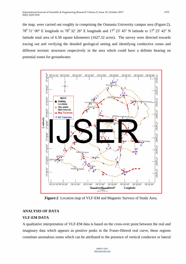
the map, were carried out roughly in comprising the Osmania University campus area (Figure:2),

780 31ʹ 00ʺ E longitude to 780 32ʹ 26ʺ E longitude and 170 23ʹ 45ʺ N latitude to 170 25ʹ 42ʺ N

latitude total area of 6.58 square kilometers (1627.32 acres). The survey were directed towards

tracing out and verifying the detailed geological setting and identifying conductive zones and

different tectonic structures respectively in the area which could have a definite bearing on

potential zones for groundwater.

Figure:2 Location map of VLF-EM and Magnetic Surveys of Study Area.

ANALYSIS OF DATA

VLF-EM DATA

A qualitative interpretation of VLF-EM data is based on the cross-over point between the real and

imaginary data which appears as positive peaks in the Fraser-filtered real curve, these regions

constitute anomalous zones which can be attributed to the presence of vertical conductor or lateral

IJSER




contacts of different resistivities beneath the surface (Srigutomo et al., 2005[4]). This, therefore,

ascertains a simple fact that the analytical signal of the real component takes off the Fraser filtered

off the real component. The Fraser Filter (Q) (Fraser, 1969[5]) was computed using a filter

operator as;

Q = (𝑸𝑸𝟒𝟒 + 𝑸𝑸𝟑𝟑) - (𝑸𝑸𝟐𝟐 + 𝑸𝑸𝟏𝟏) … (1)

Where Q is EM data and the subscript is station positions. This was applied to the real component

VLF data to transform the data set to the filtered real VLF data.

For quantitative interpretation, it is more useful to plot the real and imaginary data. The method

of estimating depth to a linear conductor based on the peak to peak width of VLF vertical in-phase

data. The depth is half the peak-to-peak width, less the instrument's elevation above ground. This

procedure was developed by Karous and Hjelt (K&H, 1983[6])

The interpretation of VLF surveys in terms of buried conductors can be assisted by the application

of the Karous and Hjelt, linear filter to the observed in-phase component of the vertical magnetic

field. Karous and Hjelt filter technique are based on discrete linear filtering of VLF data. Starting

with the Biot–Savart law to describe the magnetic field arising from a subsurface 2-D current

distribution, these authors use linear filter theory to solve the integral equation for the current

distribution, assumed to be located in a thin horizontal sheet of varying current density, situated

everywhere at a depth equal to the distance between the measurement stations. By calculating the

inverse filter at various depths (example Δx, 2Δx, 3Δx), one can study the variation of current

densities with depth. This filter is expressed as;

∆𝒛𝒛𝟐𝟐𝟐𝟐

𝑰𝑰𝒂𝒂 ∆𝒙𝒙𝟐𝟐 = 0.102 𝑯𝑯−𝟑𝟑 – 0.059 𝑯𝑯−𝟐𝟐+ 0.561 𝑯𝑯−𝟏𝟏 – 0.561 𝑯𝑯𝟏𝟏 + 0.059 𝑯𝑯𝟐𝟐 – 0.102 𝑯𝑯𝟑𝟑 … (2)

Where Δz is the assumed thickness of the current sheet, Δx is the distance between the data points

and also the depth to the current sheet, location of the calculated current density is beneath the

center point of the six data points. The values of H are the normalized vertical magnetic field

anomaly at each of six data points. Details of the filter derivation can be found in Karous & Hjelt

(1983[6]).

Filtered VLF data help to locate vertical discontinuities such as hidden faults. K&H filter

technique also provides a useful complementary tool for the semi-quantitative analysis and target

visualization from the surface to a few ten meters. The current density maxima seem always to

occur within or around the conductors. As a result of this feature, current density pseudo sections

can give diagnostic information for the target (Ogilvi and Lee, 1991[7]).

IJSER




A simple filtering technique that transforms crossovers into peaks, removes regional gradients and

also amplifies anomalies from near surface was suggested by Fraser, 1969[5]. The filter (Fraser) is

applied to the in-phase (real), Quadrature (imaginary) component data and presented in the form

of a contour map (Figure: 3 & 4). The negative contours are due to the false crossovers and are

discarded. Based on the contour pattern it may be inferred that the conductive are probably a

result of en-echelon-type complex fracture systems.

An additional interpretation tool is pseudo-section obtained through filtering (Wright, 1988[8]).

Such a section is produced by processing a given data profile with filters of various lengths. As

the length of the filter increases, response from increasing depth is successively emphasized.

Pseudo-sections are prepared for traverses AA1 to SS1 with two filters by normalizing each time

with its filter lengths of the filtered in-phase component.

TOTAL MAGNETIC DATA

Magnetic data collected in the study area are corrected for diurnal and normal correction.

Recognition of characteristic patterns and shapes of anomalies in relation to particular rock units

or geologic structures is one of the first steps in the qualitative interpretation of a magnetic map.

With the advent of detailed surveys, many near-surface geologic features are so clearly expressed

that their geologic origin is obvious in colour shaded-relief images. In the shaded-relief (Gunn,

1997[9], Davies et al., 2004[10], Gay, 2004[11]), folds look like folds, fault expressions can exhibit

en echelon and an atomizing behavior (Grauch et al., 2001[12], Langenheim et al., 2004[13]) and

individual dikes within swarms are clearly resolved (Hildenbrand and Raines, 1990[14], Modisi et

al., 2000[15]). Magnetic anomalies produced by rocks with strong, reverse-polarity eminence

display characteristic, high-amplitude negative anomalies (Books, 1962[16], Grauch et al., 1999[17])

that, without high-resolution data, might be confused with magnetic lows caused by a lack of

magnetization, which are also negative but generally featureless (Airo, 2002[18]).

The present detailed magnetic investigations make a significant contribution for the fine

elucidation of the subsurface magnetic structures in the hard rock terrain in Osmania University

campus. The following section gives detail results of qualitative and quantitative analysis of the

data.

VLF–EM AND MAGNETIC TRAVERSES

IJSER




Electromagnetic VLF magnetic traverses are carried all along parallel to the roads (15m away

from the roads) in the N-S & E-W direction. Nine (AA1, BB1, CC1, FF1, II1, NN1, OO1, QQ1 and

RR1) traverses in all were taken up. Plots of the filtered real and imaginary parts were produced

for every profile and they were interpreted in view of the existence of conductive zones that could

be related to tectonic faults.

Figures: 3 to 11 are the diagrams of the magnetic, VLF and traverses along the AA1, BB1, CC1,

FF1, II1, NN1, OO1, QQ1 and RR1respectively. From an examination of these figures we can infer

that, there is a direct correlation between magnetic (TMI) and magnetic coefficient of variation

(C.V) are responding higher values over the conductive bodies lower values over the non-

conductive bodies and they are correlated with VLF, Coefficient of variation are exactly

correlated at disturbed and fractured zones.

At locations VLF with traverses oriented in the N-S direction a plot of filtered data shows real and

imaginary components positive magnitude response intersection points resulting is probable

fractured zones located at 490 and 1850m. Comparing with the electrical sections reveals that

resistivity value of < 50Ωm are encouraging groundwater potentiality. Similarly sections FF1

comparing magnetic and VLF data oriented in the N-S direction. A well prominent three

fractured zones are delineated at 270, 390 and 500m, which exactly coincide magnetic and

magnetic coefficient of variation. And also TMI showing the low values over the conductive

bodies, high values over the non-conductive bodies.

Traverse AA1 shown in Figur.3 is running in the N-S direction about 2000m long length

extended up to west of the study area and it traverse from UFRO - under the Adikmet flyover –

PGRRCDE – EFLU – B.Ed College to Tarnaka Junction,

Total magnetic response along the traverse AA1 (Fig.3a) at 620 nT , 500 nT, -800 nT, 600 nT

and 400nT with corresponding distances 0-180m, 180-620m, 620-800m, 800-970m, and 1180-

1300m respectively. Computed Coefficient of variation along the traverse is shown in (Fig.3b)

mapped three tectonic disturbed zones marked as 1, 2 and 3.

Figure: 3(c) shows the Fraser filtered data (real or in-phase component and imaginary or

quadrature component) show positive intensities suggesting the presence of shallow and deep

conductors. This traverses is this s processed using the Karous–Hjelt filter (1983), current density

IJSER




plot for traverse as presented in Figure: 3(c) reveals a number of conductive and non conductive

subsurface structural features and inferred fractures zones (at 500, 640 and 1450m)/faults along

the traverse

In addition, to the above equivalent current density cross-section also gives an idea about the dip

direction; however, exact dip angle cannot be estimated due to the vertical axis variable being a

pseudo depth only.

The equivalence current density pseudo section of traverse (Figure:3.d) reveals the presence of

major anomalies at the southern side between 590m and 710m, and at the right side between

1400m and 1490m with depth of 20 to 60m, which can be referred to as fracture zone.

Furthermore, two high current density zones between 300m and 350m, and 510m along the

traverse can also be referred to as indications of the potential subsurface fracture system.

Traverse -

1 2 3

nT%

MA

GN

ETIC

(A)

FrFr Fr

*Fr - Fracture

VLF

-EM

(B)

(a)

(b)

(c)

(d)

IJSER




Figure: 3 Comparison of Geophysical Data with corresponding Sections for Traverses in the

Study Area (Traverse: AA1, from UFRO - under the Adikmet flyover – PGRRCDE -EFLU – B.Ed

College to Tarnaka Junction).

(a) Total Magnetic Intensity, (b) Magnetic Coefficient of variation

(c) VLF Real and Imaginary coefficents and (d) Pseudo Section

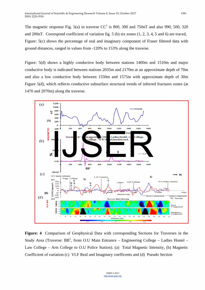
Traverse BB1 shown in Figure.4 running 2200m and trending in N-S direction , lies towards west

of the study area and it traverse from O.U Main Entrance - Engineering College - Ladies Hostel -

Law College - Arts College to O.U Police Station.

Figure: 4(a), magnetic response along the traverse at 400-600m, 1000-1100m and 1200-1300m,

magnetic response is 900, 250 and 100 nT respectively from opposite to UFRO to ‘B’ Hostel

junction road, from the geology map the highs can be inferred to correspond to a basic intrusion.

The response of coefficient of variation (Fig.4(b) a series of highs and lows zones (1, 2 and 3)

were identified , which are reflecting a low to moderate susceptibility can be attributed to the

fracture granites.

Figure: 4(c) shows the Fraser filtered data of in-phase and quadrature component, responses

ranged in value from –100 % to 175% along the traverse. Figure: 4(d) shows the corresponding

K-H pseudo section of traverse BB1. The pseudo section is a measure of the conductivity of the

subsurface as a function of depth. The conductivity shown as color codes with conductivity

increasing from left to right (i.e., from negative to positive). Different features of varying degree

of conductivity trending in different directions are delineated on the section, for instance, between

stations 515m and 620m and between stations 1745m and 1830m, highly and major conductive

bodies respectively at approximate depth of 70m are indicated. Figure: 4(a) reveals a number of

anomalies, which reflects conductive subsurface structural trends of inferred fractures zones (at

490 and 1850m) along the traverse.

Traverse CC1 shown in Figure: 5. is situated east of the O.U Campus, about 2140m long and it

runs from a point towards IPE, in N-S direction nearby Darga which is behind the Genetics Dept.

– IPE - behind the residences of Maneru Hostel to Professors Quarters.

IJSER




The magnetic response Fig. 5(a) in traverse CC1 is 800, 300 and 750nT and also 990, 500, 320

and 200nT. Correspond coefficient of variation fig. 5 (b) six zones (1, 2, 3, 4, 5 and 6) are traced,

Figure: 5(c) shows the percentage of real and imaginary component of Fraser filtered data with

ground distances, ranged in values from -120% to 153% along the traverse.

Figure: 5(d) shows a highly conductive body between stations 1400m and 1510m and major

conductive body is indicated between stations 2035m and 2170m at an approximate depth of 70m

and also a low conductive body between 1550m and 1575m with approximate depth of 30m

Figure 5(d), which reflects conductive subsurface structural trends of inferred fractures zones (at



Study Area (Traverse: BB1, from O.U Main Entrance – Engineering College – Ladies Hostel –

Law College – Arts College to O.U Police Station). (a) Total Magnetic Intensity, (b) Magnetic

Coefficient of variation (c) VLF Real and Imaginary coefficents and (d) Pseudo Section

Traverse -

(A)

VLF-

EM

(B)

nT

*Fr - Fracture

12 3

%

BB1

MA

GN

ETI

C

FrFr

(a)

(b)

(c)

(d)

IJSER




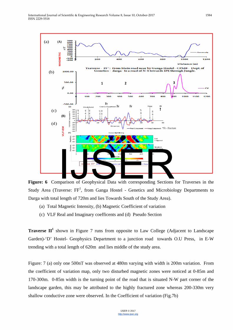
Traverse FF1 shown in Figure: 6, has the path in E-W directions and it starts from Ganga Hostel -

Genetics and Microbiology Departments to Darga - inside the Forest to a road up to a N-S

direction with total length of 1180m and lies towards south of the study area.

Here magnetic highs Fig.6 (a) at starting 0-250m and 1000m- at end of the traverse were 600nT to

700nT In between these two magnetic high minor responses are recorded. Figure: 6(b) coefficient

of variation is significant variations at 800-1000m are marked, whereas two other 200-250m, 450-

500m were noticed and three zones were identified. These two lows responses are not very clear

as the geology indicated. The highly disturbed zone were traced 800-1000m varying to 200m

width might be fault zones, and also an indication of groundwater potential zones.

IJSER





Study Area (Traverse: CC1, from a point towards IPE, in N-S direction nearby Darga which is

behind the Genetics Dept. – IPE – behind the residences of Maneru Hostel - Professors Quarters -

Indore Stadium to Aradana Theater).



Figure: 6(c) shows VLF (real and imaginary components different features of varying degree of

conductivity trending in different directions, for instance, between stations 460m and 550m, major

conductive body at an approximate depth of 70m trending in NW-SE. Highly conductive body

between stations 360m and 415m is indicated. There are several pockets of highly conductive

bodies cross-cut between stations 135m and 285m forming V-shaped conductive body.

Generally, the section shows several closures of conductive bodies at different depths. Figure:

6(d) reveals a number of anomalies, which reflects conductive subsurface structural trends of

inferred fractures zones (at 270, 390 and 500m) along the traverse.

-300.00

-200.00

-100.00

0.00

100.00

200.00

300.00

400.00

0 200 400 600 800 1000 1200 1400 1600 1800 2000 2200 2400

C.V

-2000

200400600800

10001200

0 200 400 600 800 1000 1200 1400 1600 1800 2000 2200 2400

Anomaly

Distance (m)1

2

Fr Fr

*Fr - Fracture

(A)V

LF-E

M

(B)

nT%

MA

GN

ETIC

v

v

(a)

(b)

(c)

(d)

IJSER





Study Area (Traverse: FF1, from Ganga Hostel - Genetics and Microbiology Departments to

Darga with total length of 720m and lies Towards South of the Study Area).



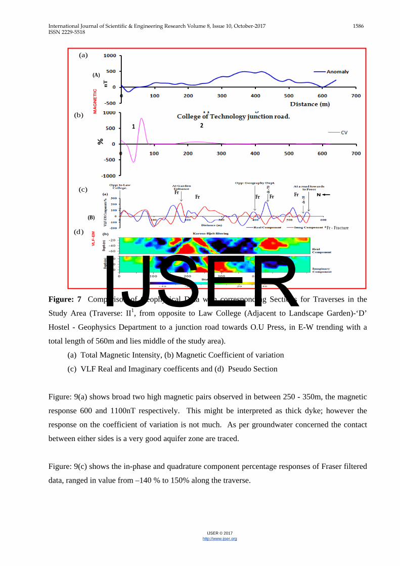
Traverse II1 shown in Figure 7 runs from opposite to Law College (Adjacent to Landscape

Garden)-‘D’ Hostel- Geophysics Department to a junction road towards O.U Press, in E-W

trending with a total length of 620m and lies middle of the study area.

Figure: 7 (a) only one 500nT was observed at 480m varying with width is 200m variation. From

the coefficient of variation map, only two disturbed magnetic zones were noticed at 0-85m and

170-300m. 0-85m width is the turning point of the road that is situated N-W part corner of the

landscape garden, this may be attributed to the highly fractured zone whereas 200-330m very

shallow conductive zone were observed. In the Coefficient of variation (Fig.7b)

31 2

nT%

VLF

-EM

MA

GN

ETI

C

FrFr

Fr

*Fr - Fracture

(A)

(B)

(a)

(b)

(c)

(d)

IJSER




Figure: 7(c) shows the anomaly response of real and imaginary Fraser filtered data, the percentage

ranged from -190% to 250%.

In figure: 7(d) different features of varying degree of conductivity are delineated on the section,

for instance, between stations 150m and 220m, and 410m and 490m major conductive bodies are

shown. Similarly, between stations 220m and 245m, and 520m and 560m, highly conductive

bodies at an approximate depth of 50m and 25m respectively present on the section. Figure:

4.13(a) reveals a number of anomalies, which reflects conductive subsurface structural trends of

inferred fractures zones (at170, 230, 410, 450 and 530m) along the traverse.

Traverse NN1 shown in Figure: 8, this 1560m and trending in an E-W direction lays towards

below middle part of the study area and it traverse from Renuka Yellamma Temple -

Administrative building - College of Technology – IPE to Dead End of the Residences Area.

The response of coefficient of variation a series of highs and lows six zones were identified

(Fig.8b), which are low to moderate susceptibility can be attributed to the fractured granite are

found in fair quantities, whereas 480 to 645m data in dyke.


ranged in value from –140 % to 150% along the traverse.

Figure: 8(d) revealed occurrence of major conductive bodies between stations 640m and 715m,

and 900m and 990m at an approximate depth of 52m and 60m respectively. There are several

pockets of highly conductive bodies are indicted along section at different depths. Figure: 8(a)

reveals a number of anomalies, which reflects conductive subsurface structural trends of inferred

fractures zones (at 700 and 1200m) along the traverse.

Traverse OO1 shown in Figure: 9 start from O.U Darga (Near Maneru Hostel) to Spot Valuation

Building running a total length of 440m to the east of study area.

IJSER





Study Area (Traverse: II1, from opposite to Law College (Adjacent to Landscape Garden)-‘D’

Hostel - Geophysics Department to a junction road towards O.U Press, in E-W trending with a

total length of 560m and lies middle of the study area).



Figure: 9(a) shows broad two high magnetic pairs observed in between 250 - 350m, the magnetic

response 600 and 1100nT respectively. This might be interpreted as thick dyke; however the

response on the coefficient of variation is not much. As per groundwater concerned the contact

between either sides is a very good aquifer zone are traced.

Figure: 9(c) shows the in-phase and quadrature component percentage responses of Fraser filtered

data, ranged in value from –140 % to 150% along the traverse.

Traverse

1 2

FrFr Fr FrFr

(A)

VLF-

EM

(B)

nT

*Fr - Fracture

%M

AG

NE

TIC

(a)

(b)

(c)

(d)

IJSER





Study Area (Traverse: NN1, from Renuka Yellamma Temple - Administrative Building - College

of Technology – IPE to Dead End of the Residences Area).



Figure: 9(d) shows a major conductive body at an approximate depth 45m between stations 340m

and 405m. Similarly, between stations 220m and 305m, a linear highly conductive body is

indicated. Figure: 9(a) reveals a number of anomalies, which reflects conductive subsurface

structural trends of inferred fractures zones (at 70 and 330m) along the traverse.

Traverse QQ1 shown in Figure.10 indicates the path in E-W direction all along the 980m length

to above middle of the study area and it starts from a junction road after Central Workshop, UCS -

Botany and Zoology Departments towards to Arts College road.

12

3 45 6

NN1

Fr Fr Fr

(A)

VL

F-E

M

(B)

nT

*Fr - Fracture

%M

AG

NE

TIC

(a)

(b)

(c)

(d)

IJSER




There are four magnetic highs Fig.10a) at distances 0-180m, 180-400m, 400-580m and 800-980m,

the magnetic response1400, 1000, 825, and 780nT respectively. Similarly the trends high and

lows were also seen on the coefficient of variation. Along this traverse five broad zones were

identified distances 0-120m, 120-250m, 335-475m, 675-820m and 820-930m correlating

interestingly opposite to the Botany Department i.e., east side of the glass room, there was a big

fracture has been traced at distance. Remaining zones were tallying the lineaments and tectonic

disturbances mapped along the traverse (Fig.10b).


Study Area (Traverse: OO1, from O.U Darga (Near Maneru Hostel) to Spot Valuation Building

running a Total length of 440m to the East of Study Area).



VL

F-E

MM

AG

NE

TIC

%

Fr Fr

*Fr - Fracture

(A)

(B)

(a)

(b)

(c)

(d)

IJSER





ranged in value from –110 % to 135% along the traverse.

Figure: 10(d) shows a major conductive body cross-cut between stations 320m and 460m forming

V-shaped conductive body. Similarly, between stations 190m and 300m, a linear major

conductive body is indicated. Generally, the section shows several closures of conductive bodies

at different depths. Figure: 10(a) reveals a number of anomalies, which reflects conductive

subsurface structural trends of inferred fractures zones (at 170, 250 and 460m) along the traverse.


Study Area (Traverse: QQ1, from A junction road after Central Workshop, UCS - Botany and

Zoology Departments to towards to Arts College Road).



Fr Fr Fr

21 3 4 5

QQ1

(A)

VLF-

EM

(B)

nT

*Fr - Fracture

%

MA

GN

ETI

C

(a)

(b)

(c)

(d)

IJSER




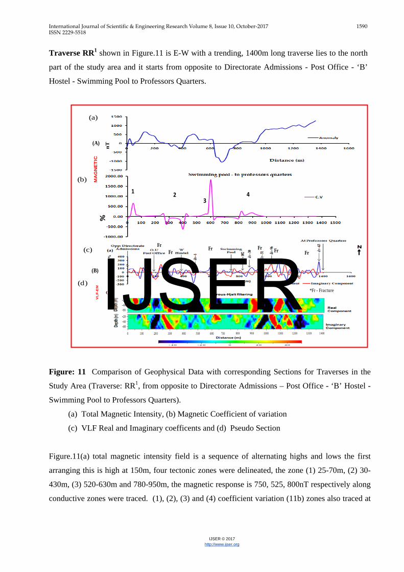
Traverse RR1 shown in Figure.11 is E-W with a trending, 1400m long traverse lies to the north

part of the study area and it starts from opposite to Directorate Admissions - Post Office - ‘B’

Hostel - Swimming Pool to Professors Quarters.


Study Area (Traverse: RR1, from opposite to Directorate Admissions – Post Office - ‘B’ Hostel -

Swimming Pool to Professors Quarters).



Figure.11(a) total magnetic intensity field is a sequence of alternating highs and lows the first

arranging this is high at 150m, four tectonic zones were delineated, the zone (1) 25-70m, (2) 30-

430m, (3) 520-630m and 780-950m, the magnetic response is 750, 525, 800nT respectively along

conductive zones were traced. (1), (2), (3) and (4) coefficient variation (11b) zones also traced at

1 23

4

RR1

FrFr

Fr Fr Fr Fr

(A)

VLF

-EM

(B)

nT

*Fr - Fracture

%M

AG

NE

TIC

(a)

(b)

(c)

(d) IJSER




the distances at the same distances coincide with the tectonically disturbed zones, whereas at

950m that is opposite to NRS hostel, a fault traced.

In Figure.11(c) different features of varying degree of conductivities are delineated on the section,

for instance, between stations 40m and 85m, 895m and 960m, 1055m and 1135m at an

approximate depth of 32m, 70m and 65m respectively. Similarly, between stations 250m and

320m, a conductive body at an approximate depth of 60m is indicated. Several other closures of

conductive bodies are present on the section. Figure 11(a) reveals a number of anomalies, which

reflects conductive subsurface structural trends of inferred fractures zones (at 240, 300, 600,950,


The results of magnetic and VLF data Figure:3, 4, 5, 7, 8, 9, 10 and 11 are representation of along

the traverses AA1, BB1, CC1, FF1, II1, NN1, OO1, QQ1 and RR1 respectively are showing similar

response of earlier traverses multi fractures are delineated, are summarized in table:1. From

figures 3 - 11 the discussion above we can qualitatively and determine the relative contribution of

magnetic and VLF methods. Two aspects emerge:

1) Magnetic and VLF methods are more sensitive to lateral and vertical litho

variations and are useful for demarcating tectonically disturbed zones and

conductive bodies which are correlative groundwater potential zones in O.U

granitic terrain.

2) The VLF method is useful because the response has real and imaginary

components from deeper horizons (Oluwafemi, O., Oladunjoye, M.A., 2013)

IJSER




Table: 1 A comparative study of information from VLF and magnetic surveys

S.No.

Traverse Identified

zones

Magnetic method

Zone width (m)

VLF Point

Remarks/Groundwater significance &aquifer

characteristic Magnetic VLF-EM

1 AA1 AA1

1 525 -820 650m Conductive/Poor 2 2 900 – 960 --- Poor 3 3 1025 – 1330 --- Very good 4

BB1 BB1 1 405 – 610 --- Very good

5 2 990 – 1100 --- Good 6 3 1215 – 1300 --- Poor 7

CC1 CC1

1 0- 105 m --- --- 8 2 185 – 300 --- --- 9 3 400 -545 --- Poor 10 4 545 – 680 --- Poor 11 5 680 -880 --- Poor 12 6 880 – 970 --- Poor 13 1 560 – 670 1455m Low Conductive/Poor 14 2 800 – 1000 567m Low Conductive/Poor 21 FF1 FF1 1 190 - 300 270m Fault/Good 28 II1 II1 1 0 -85 --- Poor 29 2 170 -300 202m ,

Conductive/Very good

41

NN1 NN1

1 200 - 350 --- Good 42 2 480 – 645 595m Dyke/Poor 43 3 645 -790 680m Conductive/Very good 44 4 890 – 1000 950m Conductive/Poor 45 5 1175 – 1300 1200m Poor 46 6 1300 – 1500 --- Poor 47 OO1 OO1 1 0-50 50m Good 48 2 135 – 270 265m Conductive/Very good 50

QQ1 QQ1

1 0 – 120 --- Poor 51 2 120 – 250 245m Conductive/Poor 52 3 335 – 475 350m,

Conductive/Poor

53 4 675 – 820 740m Lineament/Poor 54 5 820 – 930 --- Poor 55

RR1 RR1

1 25 – 70 60m Conductive/Very good 56 2 230 – 430 --- Very good/Poor 57 3 520 -630 595m dyke 58 4 780 – 950 930m Conductive/Very good

IJSER




SUMMARY AND CONCLUSIONS A qualitative analysis of vertical magnetic profiles has been performed to anticipate the

subsurface structures and rock assemblages, where groundwater aquifer zones could be possible.

From coefficient of variation profiles (Figure: 3(c) to 11 ( c) , 1, 2, 3, 4 and 5 tectonic disturbed

permeable zones were identified, which is showing as the groundwater occurence and aquifer

characteristics are magnetic response. Are showin in Table-1.

The VLF electromagnetic traversing data are presented as plots of filtered real and filtered

imaginary (in %) against station position. VLF –EM traverses from the study area are shown in

Figure 1(c) to 11(c) and these shows the linearly filtered real and imaginary components of the

vertical magnetic field of the VLF data. Figures 1 (d) to 11 (d) shows a comparison of the

Karous-Hjelt filtered real component (Karous and Hjelt, 1983).

The real and imaginary components enable qualitative identification of the top of linear features

i.e., points of coincident of crossovers and positive peaks of the real and filtered anomaly. From

these plots (Figures1 (c) - 11(c)), minor linear features suspected to be faults/fractured zones were

identified. These suspected geological interfaces are shown in the table: 1, delineated from the

profiles, was shown occurring at varying distances on the traverses. These positive peaks mapped

as fractures/conductive bodies on the filtered real are zones of interest in groundwater exploration

in hard-rock terrain. The asymmetry of these conductive anomalies suggests that the conductive

structures are dipping. Also, the anomaly patterns exhibit varying amplitudes, which are

controlled by the depth of the body to the surface, its geometry, and attitude.

A figure (from 1 (d) to 11 (d)) shows the corresponding KH filter pseudo sections of traverses

AA1-SS1. These pseudo sections are the measure of the conductivity of the subsurface as the

function of depth. The conductivity is shown as color codes. Different features of varying degree

of conductivity trending in different directions were delineated on the sections.

The VLF-EM results mapped shallow linear conductors thus are suspected fractures/conductive

bodies of varying length in the area. Also, the electrical sounding results delineated 3-4

subsurface geological layers and mapped series of basement depressions. That coincide with the

fracture zone which of significant hydro geological importance for groundwater exploration.

IJSER




ACKNOWLEDGMENT

The authors gratefully acknowledge the financial support extended by the UGC, New Delhi for

granting Emeritus fellow.

REFERENCES

[1] Satpathy, B.N. and Kanungo, B.N. 1976. Groundwater Exploration in Hard-Rock Terrain:

A Case Study. Geoph, Prosp. 24(4) pp. 725-736.

[2] Balakrishna S. and Raghava Rao M., 1961. Pink and grey granites Hyderabad, Current

Science, Vol.30, pp.264.

[3] Sitaramayya S., 1971. The Pyroxene Bearing Granodiorite and Granites of Hyderabad Area,

(the Osmania Granites): Quarterly Journal of the Geological, Mining and Metallurgical

Society of India, V.43, pp.117-129.

[4] Srigutomo, W., Harja, A., Sutarno, D. & Kagiyama, T (2005), VLF data analysis through

transformation into resistivity value: Application to synthetic and field data, Indonesia

Journal of Physics, 16(4), 127-136.

[5] Fraser, D.C., 1969, Contouring of VLF-EM data: Geophysics, Vol. 34, No. 6, p. 958- 967.

[6] Karous, M. R. and Hjelt, S. E. 1983 Linear Filtering of VLF Dip Angle Measurements.

Geophysical Prospecting, Vol. 31, pp. 782 – 794

[7] Ogilvi RD, Lee AC (1991) Interpretation of VLF-EM in-phase data using current density

psuedosections. Geophysical Prospecting, Vol 39, pp: 567–580.

[8] Wright, J.L. 1988, VLF Interpretation manual: Scintrex. Ltd

[9] Gunn, P.J., 1997, Application of aeromagnetic surveys to sedimentary basin studies:

AGSO Journal of Australian Geology and Geophysics, 17, 133-144.

[10] Davies, J., Mushayandebvu, M.F., and Smith, R., 2004, Magnetic detection and

Characterization of Tertiary and Quaternary buried channels: SEG Expanded Abstracts,

pp. 23, 734.

[11] Gay, S.P., 2004, The Meter Reader—Glacial till: A troublesome source of near-surface

magnetic anomalies: The Leading Edge, 23, 542-547.

[12] Grauch, V.J.S., Hudson, M.R., and Minor, S.A., 2001, Aeromagnetic expression of

faults that offset basin fill, Albuquerque basin, New Mexico: Geophysics, 66, 707-720.

[13] Langenheim, V.E., Jachens, R.C., Morton, D.M., Kistler, R.W., and Matti, J.C.,

2004, Geophysical and isotopic mapping of preexisting crustal structures that influenced

IJSER




the location and development of the San Jacinto fault zone, southern California: Geological

Society of America Bulletin, 116, 1143-1157.

[14] Hildenbrand, T.G., and Raines, G.L., 1990, Need for aeromagnetic data and a national

airborne geophysics program, U. S. Geological Survey Bulletin 1924, 1-5.

[15] Modisi, M.P., Atekwana, E.A., Kampunzu, A.B., and Ngwisanyi, T.H., 2000, Rift

kinematics during the incipient stages of continental extension: Evidence from the nascent

Okavango rift basin, northwest Botswana: Geology, 28, 939-942.

[16] Books, K.G., 1962, Remanent magnetism as a contributor to some aeromagnetic

anomalies: Geophysics, 27, 359-375.

[17] Grauch, V.J.S., Sawyer, D.A., Fridrich, C.J., and Hudson, M.R., 1999, Geophysical

framework of the southwestern Nevada volcanic field and hydrogeologic implications: U.S.

Geological Survey Professional Paper 1608.

[18] Airo, M.-L., 2002, Aeromagnetic and aero radiometric response to hydrothermal alteration:

Surveys in Geophysics, Vol.23, pp. 273-302

IJSER


department of geophysics, osmania university, hyderabad ijser filevlf-em and total magnetic...

Documents