descriptive statistics kenneth kwan ho chui, phd, mph department of public health and community...

Descriptive Statistics

Kenneth Kwan Ho Chui, PhD, MPHDepartment of Public Health and Community Medicine

[email protected]

Epidemiology/Biostatistics

Learning objectives in the syllabus

Distinguish between types of data

Know appropriate data presentation options for various data types

Understand the strengths and limitations of various descriptive statistics

Understand the concept of skewness and its implications to discrete and continuous distribution

Appreciate the special aspects of the normal distributions

Understand the calculation and application of z-scores

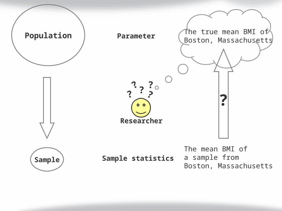
Population Parameter

Sample statisticsThe mean BMI ofa sample fromBoston, Massachusetts

The true mean BMI ofBoston, Massachusetts

? ????

Sample

Researcher

?

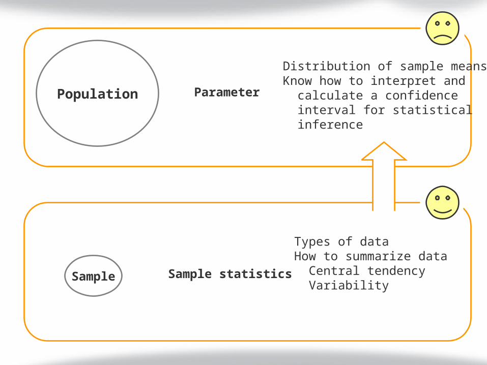
Population Parameter

Sample statisticsSample

Types of dataHow to summarize data Central tendency Variability

Distribution of sample meansKnow how to interpret and calculate a confidence interval for statistical inference

Types ofdata

Attribute Frequency

15 316 417 1218 1319 1620 2221 1522 1023 424 025 1

Mean = 19.43Median = 20.00Standard deviation = 2.01

Tabulation

Graphical visualization

Descriptive statistics

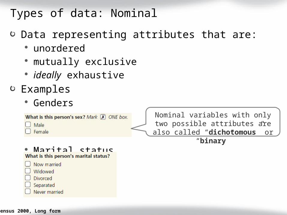
Types of data: Nominal

Data representing attributes that are: unordered mutually exclusive ideally exhaustive

Examples Genders

Marital status

Census 2000, Long form

Nominal variables with only two possible attributes are also called

“dichotomous” or “binary”

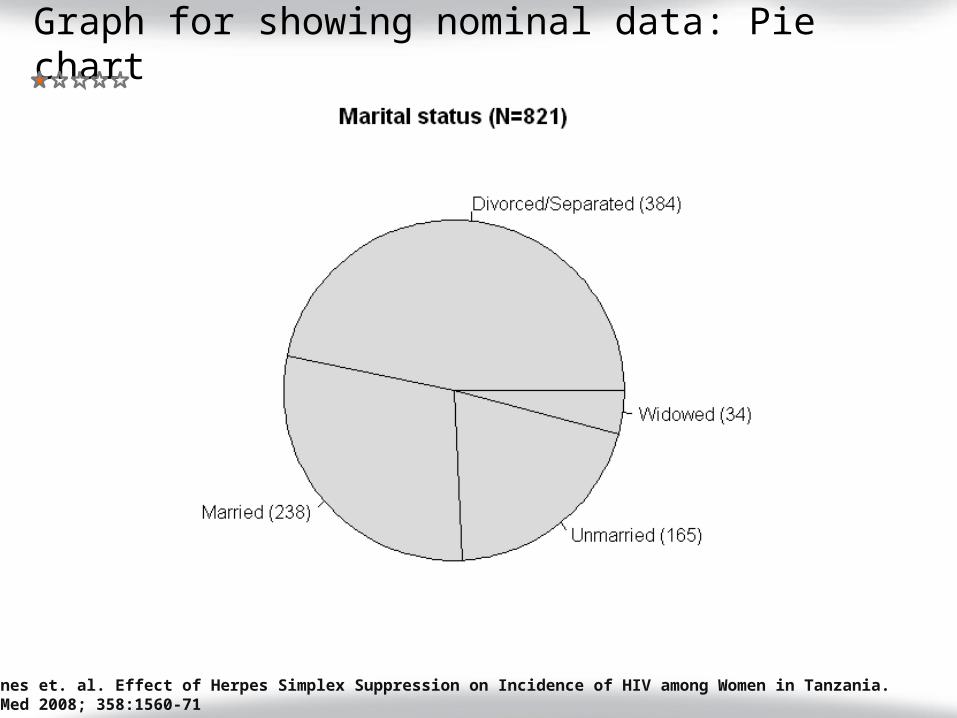
Graph for showing nominal data: Pie chart

Watson-Jones et. al. Effect of Herpes Simplex Suppression on Incidence of HIV among Women in Tanzania.N Engl J Med 2008; 358:1560-71

Graph for showing nominal data: Bar chart


Horizontal axis is categorical

Graph for showing nominal data: Grouped bar chart


Types of data: Ordinal

Data representing attributes that are: ordered unequal difference between ranks

Examples Language proficiency

Number of rooms, pay attention to the last option

Census 2000, Long form

Graph for showing oridinal data: Bar chart

US General Social Survey, 1991

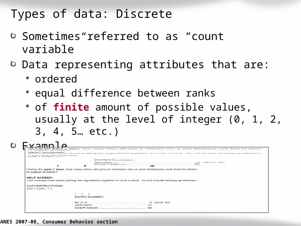
Types of data: Discrete

Sometimes referred to as “count variable”Data representing attributes that are:

ordered equal difference between ranks of finite amount of possible values, usually at

the level of integer (0, 1, 2, 3, 4, 5… etc.)

Example Frequency of cooking dinner at home

NHANES 2007-08, Consumer Behavior section

Graph for showing discrete data: Histogram


No space between bars

Horizontal axis is a continuum

Types of data: Continuous

Data representing attributes that are: ordered equal difference between ranks of infinite amount of possible values

Examples Height

Consider a reported height of 165.5 cm. In reality it could be 165.4810550654211381380… cm, so fine that we can never exactly measure it.

Blood pressure Age

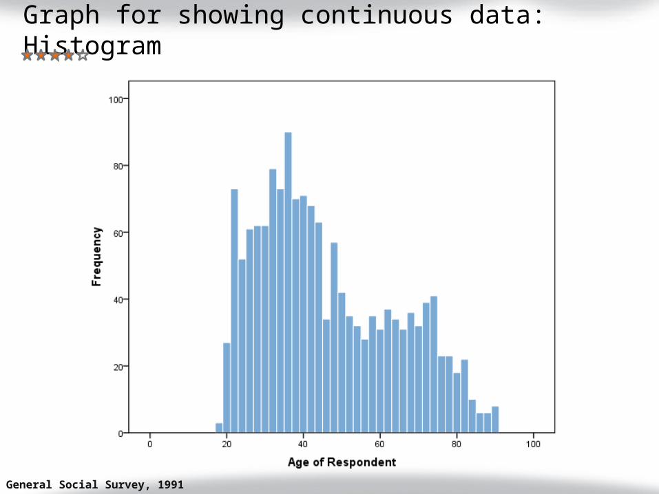
Graph for showing continuous data: Histogram


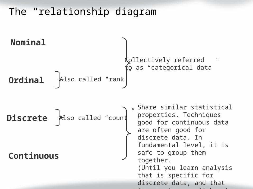
The “relationship diagram”

Nominal

Ordinal

Discrete

Continuous

Collectively referredto as “categorical data”

Also called “rank”

Share similar statistical properties. Techniques good for continuous data are often good for discrete data. In fundamental level, it is safe to group them together.(Until you learn analysis that is specific for discrete data, and that is out of our syllabus.)

Also called “count”

The hierarchy of data types

Nominal

Ordinal

Discrete

Continuous

you can themaggregate down

…but you cannotgo back up

Once the data are collected…

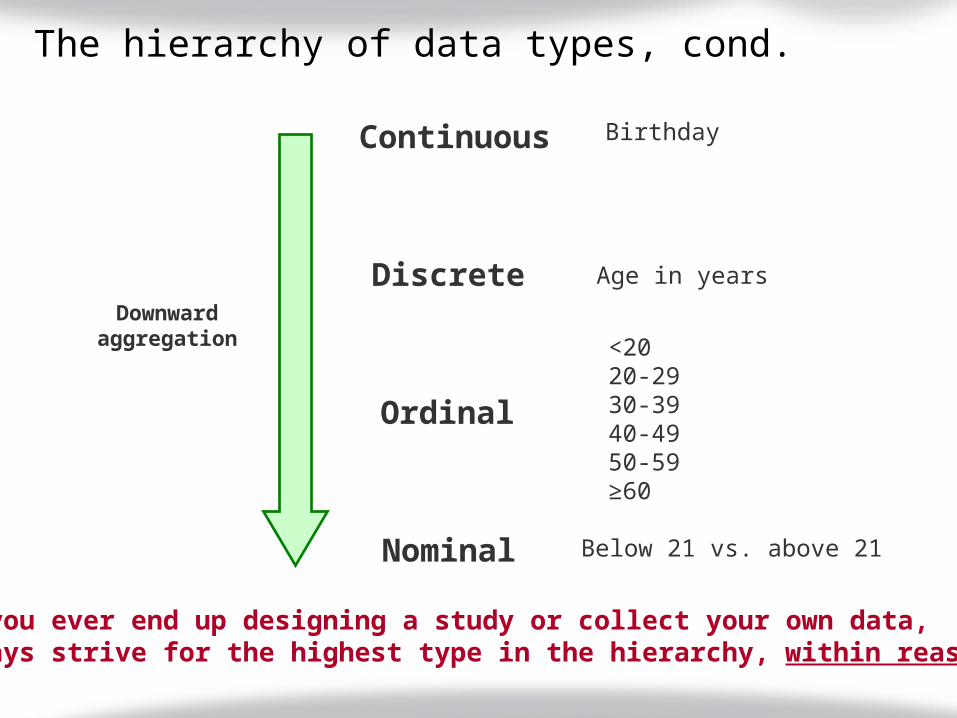
The hierarchy of data types, cond.

Nominal

Ordinal

Discrete

Continuous

Downwardaggregation

Birthday

Age in years

<2020-2930-3940-4950-59≥60

Below 21 vs. above 21

If you ever end up designing a study or collect your own data,always strive for the highest type in the hierarchy, within reason.

Centraltendency

Central tendency

The tendency of quantitative data to cluster around some central valueThree major types:Mean (also called average)Median (also called 50th percentile)Mode

Central tendency: Mean

Consider a variable with data:1, 2, 3, 3, 4, 4, 4, 5, 5, 6

Central tendency: Median

A median is the numeric value separating the higher half of a sample from the lower halfMedian can be found by:1. Arranging all the observations in ascending or

descending order2. Picking the middle number as the median3. If there is an even number of observations,

then the median is the mean of the two middle values

Consider a variable with data:1, 2, 3, 3, 4, 4, 4, 5, 5, 6Since we have even number of cases, the median is then the mean of the two middle values, which is(4+4)/2 = 4

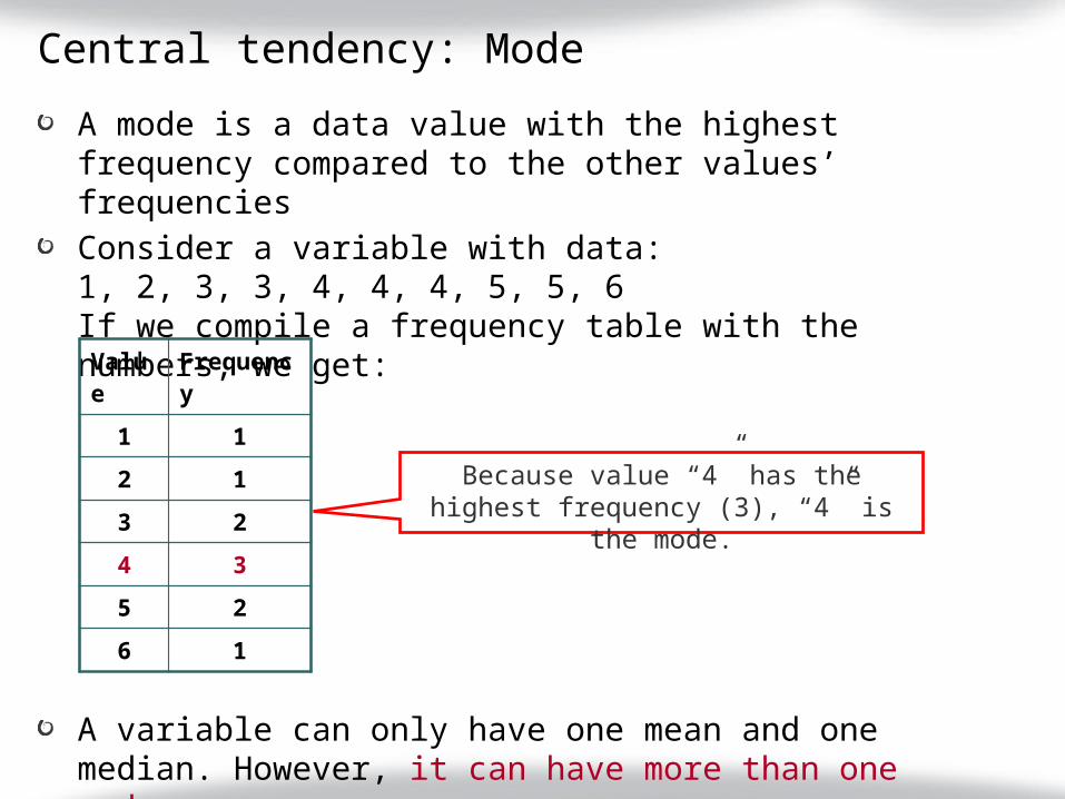
Central tendency: Mode

A mode is a data value with the highest frequency compared to the other values’ frequenciesConsider a variable with data:1, 2, 3, 3, 4, 4, 4, 5, 5, 6If we compile a frequency table with the numbers, we get:

A variable can only have one mean and one median. However, it can have more than one mode.

Value

Frequency

1 1

2 1

3 2

4 3

5 2

6 1

Because value “4” has the highest frequency (3), “4” is the mode.

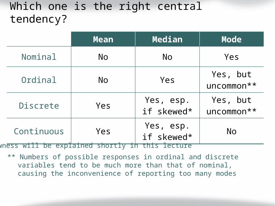
Which one is the right central tendency?

Mean Median Mode

Nominal No No Yes

Ordinal No Yes Yes, but uncommon**

Discrete Yes Yes, esp. if skewed*

Yes, but uncommon**

Continuous Yes Yes, esp. if skewed* No

* Skewness will be explained shortly in this lecture

** Numbers of possible responses in ordinal and discrete variables tend to be much more than that of nominal, causing the inconvenience of reporting too many modes

Variability

Variability

The magnitude of dispersion of the data around their own central valueFour major expressions:RangeInterquartile range (IQR)VarianceStandard deviation

Variability: Range

A range is the difference between the smallest and the largest values in a variableConsider a variable with data:1, 2, 3, 3, 4, 4, 4, 5, 5, 6The range is (6 – 1) = 5No conventional way of pairing with any particular central tendency measure

Variability: Interquartile range

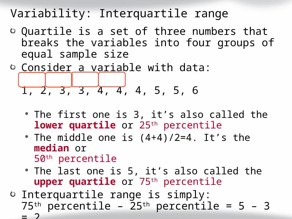
Quartile is a set of three numbers that breaks the variables into four groups of equal sample sizeConsider a variable with data:

1, 2, 3, 3, 4, 4, 4, 5, 5, 6

The first one is 3, it’s also called the lower quartile or 25th percentile

The middle one is (4+4)/2=4. It’s the median or50th percentile

The last one is 5, it’s also called the upper quartile or 75th percentile

Interquartile range is simply:75th percentile – 25th percentile = 5 – 3 = 2Often paired with median in data reporting

A little caveat about quartiles

The median is well defined, but there has not been a universal agreement on how the upper and lower quartiles should be derived.Two examples:

1, 2, 3, 41, 2

3, 4

1, 2, 3, 41, 2, 2.5

2.5, 3, 4

Lower quartile: 1.5

Upper quartile: 3.5

Lower quartile: 2

Upper quartile: 3

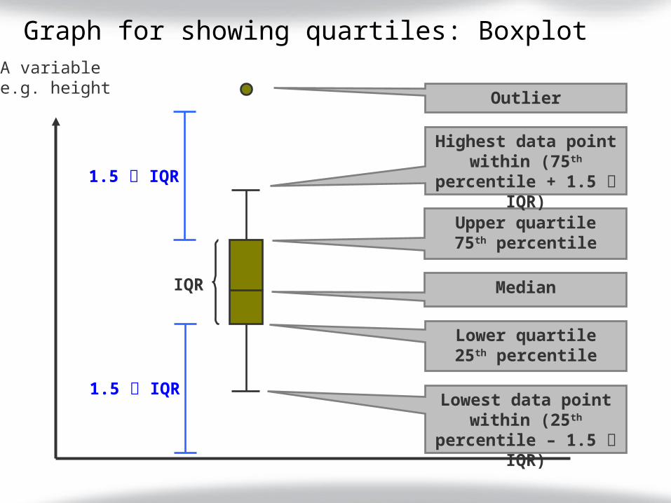
Graph for showing quartiles: BoxplotA variablee.g. height

Median

Upper quartile75th percentile

Lower quartile25th percentile

IQR

Outlier

Highest data point within (75th

percentile + 1.5 IQR)

1.5 IQR

Lowest data point within (25th

percentile – 1.5 IQR)

1.5 IQR

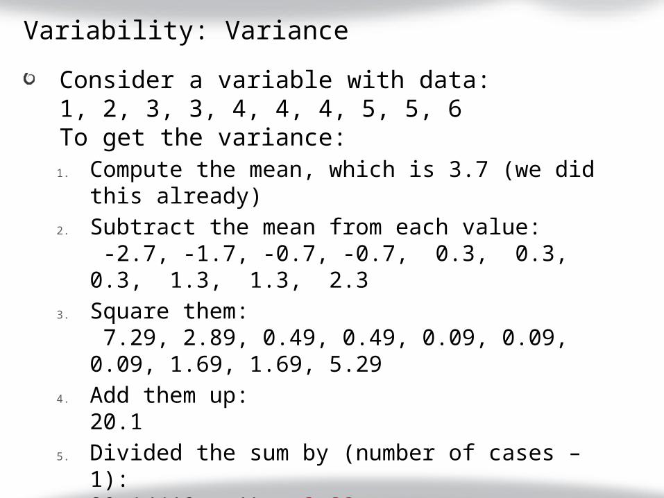
Variability: Variance

Consider a variable with data:1, 2, 3, 3, 4, 4, 4, 5, 5, 6To get the variance:1. Compute the mean, which is 3.7 (we did this

already)2. Subtract the mean from each value:

-2.7, -1.7, -0.7, -0.7, 0.3, 0.3, 0.3, 1.3, 1.3, 2.3

3. Square them: 7.29, 2.89, 0.49, 0.49, 0.09, 0.09, 0.09, 1.69, 1.69, 5.29

4. Add them up:20.1

5. Divided the sum by (number of cases – 1):20.1/(10 – 1) = 2.23

Fortunately, computer can now do all these for us!

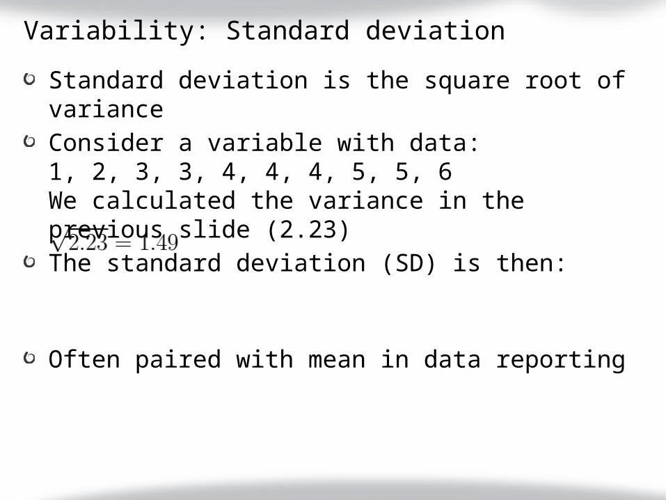
Variability: Standard deviation

Standard deviation is the square root of varianceConsider a variable with data:1, 2, 3, 3, 4, 4, 4, 5, 5, 6We calculated the variance in the previous slide (2.23)The standard deviation (SD) is then:

Often paired with mean in data reporting

Which one is the right variability?

Range IQR* Variance SD*

Nominal No No No

Ordinal Yes Yes No

Discrete Yes Yes, esp. if skewed** Yes

Continuous Yes Yes, esp. if

skewed** Yes

* IQR: Interquartile range; SD: Standard deviation

** Skewness will be explained shortly in this lecture

Normaldistribution

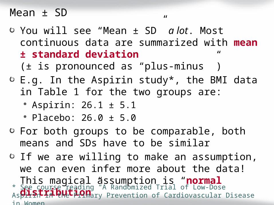
Mean ± SD

You will see “Mean ± SD” a lot. Most continuous data are summarized with mean ± standard deviation(± is pronounced as “plus-minus ”) E.g. In the Aspirin study*, the BMI data in Table 1 for the two groups are:

Aspirin: 26.1 ± 5.1 Placebo: 26.0 ± 5.0

For both groups to be comparable, both means and SDs have to be similarIf we are willing to make an assumption, we can even infer more about the data! This magical assumption is “normal distribution”

* See course reading “A Randomized Trial of Low-Dose Aspirin in the Primary Prevention of Cardiovascular Disease in Women”

Normal distribution

Some variables, when plotted in the form of a histogram, look like this:

Reasonably symmetric

More values at the center

Decreasing number of values towards the two ends

Looks like a bell

When this happens, we can say a lot more with the mean and standard deviation!

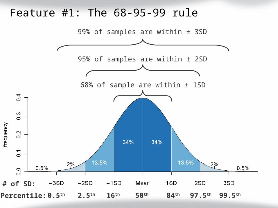
Feature #1: The 68-95-99 rule

68% of sample are within ± 1SD

95% of samples are within ± 2SD

99% of samples are within ± 3SD

50th 84th 97.5th 99.5th16th2.5th0.5thPercentile:

# of SD:

Application of the 68-95-99 rule (I)

The mean (±SD) of the daily caloric intake of a certain group is 1200 ± 150ASSUME THE VARIABLE DAILY CALORIC INTAKE IS NORMALLY DISTRIBUTED*, then:

68% of the participants have caloric intakes ranging from 1050 to 1350 kcal (– 1 SD to 1 SD)



* This assumption is needed for the 68-95-99 rule to work. The distribution can be checked with histogram or other statistics(not covered in this class)

Application of the 68-95-99 rule (II)

The mean (±SD) of the daily caloric intake of a certain group is 1200 ± 150ASSUME THE VARIABLE DAILY CALORIC INTAKE IS NORMALLY DISTRIBUTED*, then:

The data point at the 84th percentile is about(1200 + 150) = 1350 kcal

The data point at the 99.5th percentile is about(1200 + 450) = 1650 kcal

A subject with kcal = 1200 is likely to be the 50th percentile in this sample

* This assumption is needed for the 68-95-99 rule to work. The distribution can be checked with histogram or other statistics(not covered in this class)

Feature #2: Standardized comparison with z-score

Consider an imaginary sample Height: Mean = 160 cm, SD = 15 cm Weight: Mean = 95 lb, SD = 10 lb

How is someone who is 180 cm tall and 107 lb heavy doing relative to the rest? The different units are impeding direct comparison, but z-score can help

i.e. z-score is simply how many SDs a value is away from the meanz-score for the person’s height: (180 – 160)/15 = 1.33z-score for the person’s weight: (107 – 95)/10 = 0.70

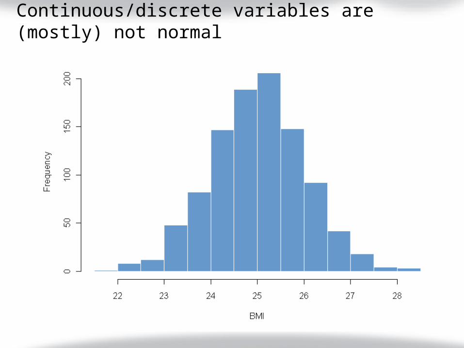
Continuous/discrete variables are (mostly) not normal

Problems with skewed distribution

Mean & Median

Problems with skewed distributionsMeanMedian MedianMean

Positively skewed/Right skewedMedian is more or less the sameIQR is more or less the sameMean becomes largerSD is inflated

Negatively skewed/Left skewedMedian is more or less the sameIQR is more or less the sameMean becomes smallerSD is inflated

For variables with a skewed distribution, median & interquartile range is a better representation of the central tendency and variability, respectively

Tell-tale signs of skewness

When the mean and median of the variable are very differentWhen you try to reconstruct the histogram of the normal distribution for the variable, a good part of the curve falls into an illogical or biologically implausible domain:

In a study with an entry criteria of age ≥ 45, the mean and standard deviation of the age is 52.0±7.0

A study on eating out reported that an average family makes dinner at home on 5.2±2.0 nights/week

When the authors reported only median with/without quartiles for the variable

Skewness distorts the means, and hence distorts analyses that heavily rely on the sample meansAsk if the skewness is relevant

For some variables in statistical analysis, we don’t care as much if they are skewed or not

Ask if the skewness is serious Some analyses are robust enough to tolerate

some skewness

Check if the authors employed solutions such as:

Transformation (e.g. logarithmic, square root, etc.)

Aggregating down the data type hierarchy Using analyses that have relaxed requirement

on the sample’s distribution (e.g. non-parametric procedures)

So what if it’s skewed? (Advanced teaser)

descriptive statistics kenneth kwan ho chui, phd, mph department of public health and community...

Documents

types of data slide

nominal data

discrete data

continuous data

oridinal data

ordinal data

various data types

scores slide