descriptive statistics: numerical measures -...
TRANSCRIPT

Descriptive Statistics:Numerical Measures
CONTENTS
STATISTICS IN PRACTICE: SMALL FRY DESIGN
3.1 MEASURES OF LOCATIONMeanMedianModePercentilesQuartiles
3.2 MEASURES OF VARIABILITYRangeInterquartile RangeVarianceStandard DeviationCoefficient of Variation
3.3 MEASURES OFDISTRIBUTION SHAPE,RELATIVE LOCATION, ANDDETECTING OUTLIERSDistribution Shapez-Scores
Chebyshev’s TheoremEmpirical RuleDetecting Outliers
3.4 EXPLORATORY DATAANALYSISFive-Number SummaryBox Plot
3.5 MEASURES OFASSOCIATION BETWEENTWO VARIABLESCovarianceInterpretation of the CovarianceCorrelation CoefficientInterpretation of the Correlation
Coefficient
3.6 THE WEIGHTED MEAN ANDWORKING WITH GROUPEDDATAWeighted MeanGrouped Data
CHAPTER 3
Openmirrors.com

86 Chapter 3 Descriptive Statistics: Numerical Measures
MAC PULL IN ART HERE, adjust size
as needed.
STATISTICS in PRACTICE
Founded in 1997, Small Fry Design is a toy and acces-sory company that designs and imports products for in-fants. The company’s product line includes teddy bears,mobiles, musical toys, rattles, and security blankets andfeatures high-quality soft toy designs with an emphasison color, texture, and sound. The products are designedin the United States and manufactured in China.
Small Fry Design uses independent representativesto sell the products to infant furnishing retailers, chil-dren’s accessory and apparel stores, gift shops, upscaledepartment stores, and major catalog companies. Cur-rently, Small Fry Design products are distributed in morethan 1000 retail outlets throughout the United States.
Cash flow management is one of the most critical ac-tivities in the day-to-day operation of this company. En-suring sufficient incoming cash to meet both current andongoing debt obligations can mean the difference betweenbusiness success and failure. A critical factor in cash flowmanagement is the analysis and control of accounts re-ceivable. By measuring the average age and dollar valueof outstanding invoices, management can predict cashavailability and monitor changes in the status of accountsreceivable. The company set the following goals: the av-erage age for outstanding invoices should not exceed 45days, and the dollar value of invoices more than 60 daysold should not exceed 5% of the dollar value of all ac-counts receivable.
In a recent summary of accounts receivable status,the following descriptive statistics were provided for theage of outstanding invoices:
Mean 40 daysMedian 35 daysMode 31 days
Interpretation of these statistics shows that the mean or av-erage age of an invoice is 40 days. The median shows thathalf of the invoices remain outstanding 35 days or more.The mode of 31 days, the most frequent invoice age, indi-cates that the most common length of time an invoice isoutstanding is 31 days. The statistical summary alsoshowed that only 3% of the dollar value of all accounts re-ceivable was more than 60 days old. Based on the statisti-cal information, management was satisfied that accountsreceivable and incoming cash flow were under control.
In this chapter, you will learn how to compute andinterpret some of the statistical measures used by SmallFry Design. In addition to the mean, median, and mode,you will learn about other descriptive statistics such asthe range, variance, standard deviation, percentiles, andcorrelation. These numerical measures will assist in theunderstanding and interpretation of data.
Small Fry Design’s “King of the Jungle” mobile. © Joe-Higgins/South-Western.
SMALL FRY DESIGN*SANTA ANA, CALIFORNIA
STATISTICS in PRACTICE
*The authors are indebted to John A. McCarthy, President of Small FryDesign, for providing this Statistics in Practice.
In Chapter 2 we discussed tabular and graphical presentations used to summarize data. Inthis chapter, we present several numerical measures that provide additional alternatives forsummarizing data.
We start by developing numerical summary measures for data sets consisting of a sin-gle variable. When a data set contains more than one variable, the same numerical measurescan be computed separately for each variable. However, in the two-variable case, we willalso develop measures of the relationship between the variables.

3.1 Measures of Location 87
SAMPLE MEAN
(3.1)x ��xi
n
The sample mean is asample statistic.
x
Numerical measures of location, dispersion, shape, and association are introduced. Ifthe measures are computed for data from a sample, they are called sample statistics. If themeasures are computed for data from a population, they are called population parameters.In statistical inference, a sample statistic is referred to as the point estimator of the corre-sponding population parameter. In Chapter 7 we will discuss in more detail the process ofpoint estimation.
In the three chapter appendixes we show how Minitab, Excel, and StatTools can be usedto compute the numerical measures described in the chapter.
3.1 Measures of LocationMeanPerhaps the most important measure of location is the mean, or average value, for a vari-able. The mean provides a measure of central location for the data. If the data are for asample, the mean is denoted by ; if the data are for a population, the mean is denoted bythe Greek letter μ.
In statistical formulas, it is customary to denote the value of variable x for the first ob-servation by x1, the value of variable x for the second observation by x2, and so on. In gen-eral, the value of variable x for the ith observation is denoted by xi. For a sample with nobservations, the formula for the sample mean is as follows.
x
In the preceding formula, the numerator is the sum of the values of the n observations. That is,
The Greek letter � is the summation sign.To illustrate the computation of a sample mean, let us consider the following class size
data for a sample of five college classes.
We use the notation x1, x2, x3, x4, x5 to represent the number of students in each of the five classes.
Hence, to compute the sample mean, we can write
The sample mean class size is 44 students.Another illustration of the computation of a sample mean is given in the following situ-
ation. Suppose that a college placement office sent a questionnaire to a sample of businessschool graduates requesting information on monthly starting salaries. Table 3.1 shows the
x ��xi
n�
x1 � x2 � x3 � x4 � x5
5�
46 � 54 � 42 � 46 � 32
5� 44
x1 � 46 x2 � 54 x3 � 42 x4 � 46 x5 � 32
46 54 42 46 32
�xi � x1 � x2 � . . . � xn

88 Chapter 3 Descriptive Statistics: Numerical Measures
POPULATION MEAN
(3.2)μ ��xi
N
The sample mean x is apoint estimator of thepopulation mean μ.
collected data. The mean monthly starting salary for the sample of 12 business collegegraduates is computed as
Equation (3.1) shows how the mean is computed for a sample with n observations. Theformula for computing the mean of a population remains the same, but we use differentnotation to indicate that we are working with the entire population. The number of obser-vations in a population is denoted by N and the symbol for a population mean is μ.
�42,480
12� 3540
�3450 � 3550 � . . . � 3480
12
x ��xi
n�
x1 � x2 � . . . � x12
12
MedianThe median is another measure of central location. The median is the value in the middlewhen the data are arranged in ascending order (smallest value to largest value). With an oddnumber of observations, the median is the middle value. An even number of observationshas no single middle value. In this case, we follow convention and define the median as theaverage of the values for the middle two observations. For convenience the definition of themedian is restated as follows.
Monthly MonthlyGraduate Starting Salary ($) Graduate Starting Salary ($)
1 3450 7 34902 3550 8 37303 3650 9 35404 3480 10 39255 3355 11 35206 3310 12 3480
TABLE 3.1 MONTHLY STARTING SALARIES FOR A SAMPLE OF 12 BUSINESS SCHOOLGRADUATES
MEDIAN
Arrange the data in ascending order (smallest value to largest value).
(a) For an odd number of observations, the median is the middle value.(b) For an even number of observations, the median is the average of the two
middle values.
fileWEBStartSalary

3.1 Measures of Location 89
Let us apply this definition to compute the median class size for the sample of five collegeclasses. Arranging the data in ascending order provides the following list.
Because n � 5 is odd, the median is the middle value. Thus the median class size is 46 stu-dents. Even though this data set contains two observations with values of 46, each obser-vation is treated separately when we arrange the data in ascending order.
Suppose we also compute the median starting salary for the 12 business college gradu-ates in Table 3.1. We first arrange the data in ascending order.
3310 3355 3450 3480 3480 3490 3520 3540 3550 3650 3730 392514243
Middle Two Values
Because n � 12 is even, we identify the middle two values: 3490 and 3520. The median isthe average of these values.
Although the mean is the more commonly used measure of central location, in somesituations the median is preferred. The mean is influenced by extremely small and large datavalues. For instance, suppose that one of the graduates (see Table 3.1) had a starting salaryof $10,000 per month (maybe the individual’s family owns the company). If we change thehighest monthly starting salary in Table 3.1 from $3925 to $10,000 and recompute themean, the sample mean changes from $3540 to $4046. The median of $3505, however, isunchanged, because $3490 and $3520 are still the middle two values. With the extremelyhigh starting salary included, the median provides a better measure of central location thanthe mean. We can generalize to say that whenever a data set contains extreme values, themedian is often the preferred measure of central location.
ModeA third measure of location is the mode. The mode is defined as follows.
Median �3490 � 3520
2� 3505
32 42 46 46 54
To illustrate the identification of the mode, consider the sample of five class sizes. Theonly value that occurs more than once is 46. Because this value, occurring with a fre-quency of 2, has the greatest frequency, it is the mode. As another illustration, consider thesample of starting salaries for the business school graduates. The only monthly startingsalary that occurs more than once is $3480. Because this value has the greatest frequency, itis the mode.
Situations can arise for which the greatest frequency occurs at two or more differentvalues. In these instances more than one mode exists. If the data contain exactly two modes,we say that the data are bimodal. If data contain more than two modes, we say that the dataare multimodal. In multimodal cases the mode is almost never reported because listing threeor more modes would not be particularly helpful in describing a location for the data.
The median is the measureof location most oftenreported for annual incomeand property value databecause a few extremelylarge incomes or propertyvalues can inflate the mean.In such cases, the median isthe preferred measure ofcentral location.
MODE
The mode is the value that occurs with greatest frequency.

90 Chapter 3 Descriptive Statistics: Numerical Measures
PercentilesA percentile provides information about how the data are spread over the interval from thesmallest value to the largest value. For data that do not contain numerous repeated values,the pth percentile divides the data into two parts. Approximately p percent of the observa-tions have values less than the pth percentile; approximately (100 � p) percent of the ob-servations have values greater than the pth percentile. The pth percentile is formally definedas follows.
Colleges and universities frequently report admission test scores in terms of percentiles.For instance, suppose an applicant obtains a raw score of 54 on the verbal portion of an ad-mission test. How this student performed in relation to other students taking the same testmay not be readily apparent. However, if the raw score of 54 corresponds to the 70th per-centile, we know that approximately 70% of the students scored lower than this individualand approximately 30% of the students scored higher than this individual.
The following procedure can be used to compute the pth percentile.
PERCENTILE
The pth percentile is a value such that at least p percent of the observations are lessthan or equal to this value and at least (100 � p) percent of the observations aregreater than or equal to this value.
CALCULATING THE pTH PERCENTILE
Step 1. Arrange the data in ascending order (smallest value to largest value).Step 2. Compute an index i
where p is the percentile of interest and n is the number of observations.Step 3. (a) If i is not an integer, round up. The next integer greater than i denotes
the position of the pth percentile.(b) If i is an integer, the pth percentile is the average of the values in po-sitions i and i � 1.
i � � p
100�n
Following these stepsmakes it easy to calculatepercentiles.
As an illustration of this procedure, let us determine the 85th percentile for the startingsalary data in Table 3.1.
Step 1. Arrange the data in ascending order.
Step 2.
Step 3. Because i is not an integer, round up. The position of the 85th percentile is thenext integer greater than 10.2, the 11th position.
Returning to the data, we see that the 85th percentile is the data value in the 11th position,or 3730.
i � � p
100�n � � 85
100�12 � 10.2
3310 3355 3450 3480 3480 3490 3520 3540 3550 3650 3730 3925

3.1 Measures of Location 91
Q1 Q2 Q3
25% 25%25%25%
First Quartile(25th percentile)
Second Quartile(50th percentile)
(median)
Third Quartile(75th percentile)
FIGURE 3.1 LOCATION OF THE QUARTILES
As another illustration of this procedure, let us consider the calculation of the 50th per-centile for the starting salary data. Applying step 2, we obtain
Because i is an integer, step 3(b) states that the 50th percentile is the average of the sixthand seventh data values; thus the 50th percentile is (3490 � 3520)/2 � 3505. Note that the50th percentile is also the median.
QuartilesIt is often desirable to divide data into four parts, with each part containing approximatelyone-fourth, or 25% of the observations. Figure 3.1 shows a data distribution divided intofour parts. The division points are referred to as the quartiles and are defined as
The starting salary data are again arranged in ascending order. We already identified Q2,the second quartile (median), as 3505.
The computations of quartiles Q1 and Q3 require the use of the rule for finding the 25th and75th percentiles. These calculations follow.
For Q1,
Because i is an integer, step 3(b) indicates that the first quartile, or 25th percentile, is theaverage of the third and fourth data values; thus, Q1 � (3450 � 3480)/2 � 3465.
For Q3,
Again, because i is an integer, step 3(b) indicates that the third quartile, or 75th percentile,is the average of the ninth and tenth data values; thus, Q3 � (3550 � 3650)/2 � 3600.
i � � p
100�n � � 75
100�12 � 9
i � � p
100�n � � 25
100�12 � 3
3310 3355 3450 3480 3480 3490 3520 3540 3550 3650 3730 3925
Q3 � third quartile, or 75th percentile.
Q2 � second quartile, or 50th percentile (also the median)
Q1 � first quartile, or 25th percentile
i � � 50
100�12 � 6
Quartiles are just specificpercentiles; thus, the stepsfor computing percentilescan be applied directly inthe computation ofquartiles.

92 Chapter 3 Descriptive Statistics: Numerical Measures
The quartiles divide the starting salary data into four parts, with each part containing25% of the observations.
3310 3355 3450 3480 3480 3490 3520 3540 3550 3650 3730 3925
We defined the quartiles as the 25th, 50th, and 75th percentiles. Thus, we computed thequartiles in the same way as percentiles. However, other conventions are sometimes usedto compute quartiles, and the actual values reported for quartiles may vary slightly de-pending on the convention used. Nevertheless, the objective of all procedures for comput-ing quartiles is to divide the data into four equal parts.
(Median)Q3 � 3600Q2 � 3505Q1 � 3465
���
moving the smallest 5% and the largest 5% of thedata values and then computing the mean of theremaining values. Using the sample with n � 12starting salaries, 0.05(12) � 0.6. Rounding this valueto 1 indicates that the 5% trimmed mean wouldremove the 1 smallest data value and the 1 largestdata value. The 5% trimmed mean using the 10 re-maining observations is 3524.50.
NOTES AND COMMENTS
It is better to use the median than the mean as ameasure of central location when a data set con-tains extreme values. Another measure, sometimesused when extreme values are present, is the trimmedmean. It is obtained by deleting a percentage of thesmallest and largest values from a data set and thencomputing the mean of the remaining values. Forexample, the 5% trimmed mean is obtained by re-
Exercises
Methods1. Consider a sample with data values of 10, 20, 12, 17, and 16. Compute the mean and median.
2. Consider a sample with data values of 10, 20, 21, 17, 16, and 12. Compute the mean andmedian.
3. Consider a sample with data values of 27, 25, 20, 15, 30, 34, 28, and 25. Compute the 20th,25th, 65th, and 75th percentiles.
4. Consider a sample with data values of 53, 55, 70, 58, 64, 57, 53, 69, 57, 68, and 53. Com-pute the mean, median, and mode.
Applications5. The Dow Jones Travel Index reported what business travelers pay for hotel rooms per night
in major U.S. cities (The Wall Street Journal, January 16, 2004). The average hotel roomrates for 20 cities are as follows:
Atlanta $163 Minneapolis $125Boston 177 New Orleans 167Chicago 166 New York 245Cleveland 126 Orlando 146Dallas 123 Phoenix 139Denver 120 Pittsburgh 134Detroit 144 San Francisco 167Houston 173 Seattle 162Los Angeles 160 St. Louis 145Miami 192 Washington, D.C. 207
testSELF
fileWEBHotels

3.1 Measures of Location 93
a. What is the mean hotel room rate?b. What is the median hotel room rate?c. What is the mode?d. What is the first quartile?e. What is the third quartile?
6. During the 2007–2008 NCAAcollege basketball season, men’s basketball teams attemptedan all-time high number of 3-point shots, averaging 19.07 shots per game (AssociatedPress Sports, January 24, 2009). In an attempt to discourage so many 3-point shots and encourage more inside play, the NCAA rules committee moved the 3-point line back from19 feet, 9 inches to 20 feet, 9 inches at the beginning of the 2008–2009 basketball season.Shown in the following table are the 3-point shots taken and the 3-point shots made for asample of 19 NCAA basketball games during the 2008–2009 season.
fileWEB3Points
3-Point Shots Shots Made 3-Point Shots Shots Made
23 4 17 720 6 19 1017 5 22 718 8 25 1113 4 15 616 4 10 58 5 11 3
19 8 25 828 5 23 721 7
a. What is the mean number of 3-point shots taken per game?b. What is the mean number of 3-point shots made per game?c. Using the closer 3-point line, players were making 35.2% of their shots. What per-
centage of shots were players making from the new 3-point line?d. What was the impact of the NCAA rules change that moved the 3-point line back to
20 feet, 9 inches for the 2008–2009 season? Would you agree with the AssociatedPress Sports article that stated, “Moving back the 3-point line hasn’t changed the gamedramatically”? Explain.
7. Endowment income is a critical part of the annual budgets at colleges and universities.A study by the National Association of College and University Business Officers re-ported that the 435 colleges and universities surveyed held a total of $413 billion in en-dowments. The 10 wealthiest universities are shown below (The Wall Street Journal,January 27, 2009). Amounts are in billion of dollars.
a. What is the mean endowment for these universities?b. What is the median endowment?c. What is the mode endowment?d. Compute the first and third quartiles?
University Endowment ($billion) University Endowment ($billion)
Columbia 7.2 Princeton 16.4Harvard 36.6 Stanford 17.2M.I.T. 10.1 Texas 16.1Michigan 7.6 Texas A&M 6.7Northwestern 7.2 Yale 22.9
94 Chapter 3 Descriptive Statistics: Numerical Measures
e. What is the total endowment at these 10 universities? These universities represent2.3% of the 435 colleges and universities surveyed. What percentage of the total $413billion in endowments is held by these 10 universities?
f. The Wall Street Journal reported that over a recent five-month period, a downturn in the economy has caused endowments to decline 23%. What is the estimate of thedollar amount of the decline in the total endowments held by these 10 universities?Given this situation, what are some of the steps you would expect university admin-istrators to be considering?
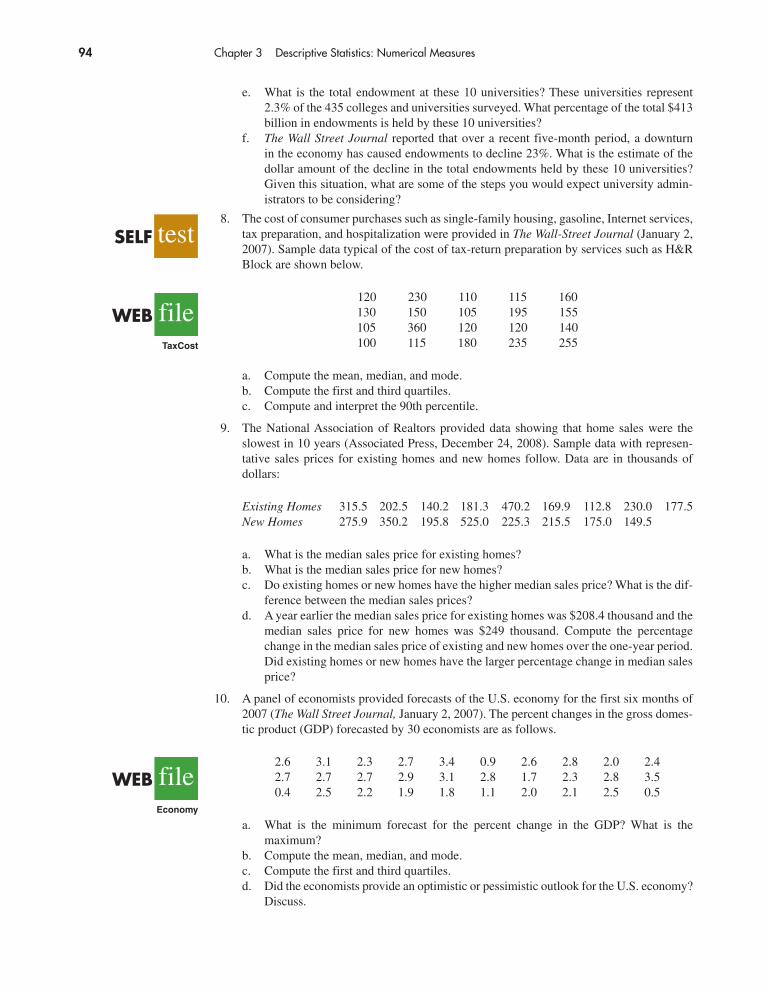
8. The cost of consumer purchases such as single-family housing, gasoline, Internet services,tax preparation, and hospitalization were provided in The Wall-Street Journal (January 2,2007). Sample data typical of the cost of tax-return preparation by services such as H&RBlock are shown below.
120 230 110 115 160130 150 105 195 155105 360 120 120 140100 115 180 235 255
a. Compute the mean, median, and mode.b. Compute the first and third quartiles.c. Compute and interpret the 90th percentile.
9. The National Association of Realtors provided data showing that home sales were theslowest in 10 years (Associated Press, December 24, 2008). Sample data with represen-tative sales prices for existing homes and new homes follow. Data are in thousands ofdollars:
Existing Homes 315.5 202.5 140.2 181.3 470.2 169.9 112.8 230.0 177.5New Homes 275.9 350.2 195.8 525.0 225.3 215.5 175.0 149.5
a. What is the median sales price for existing homes?b. What is the median sales price for new homes?c. Do existing homes or new homes have the higher median sales price? What is the dif-
ference between the median sales prices?d. A year earlier the median sales price for existing homes was $208.4 thousand and the
median sales price for new homes was $249 thousand. Compute the percentagechange in the median sales price of existing and new homes over the one-year period.Did existing homes or new homes have the larger percentage change in median salesprice?
10. A panel of economists provided forecasts of the U.S. economy for the first six months of2007 (The Wall Street Journal, January 2, 2007). The percent changes in the gross domes-tic product (GDP) forecasted by 30 economists are as follows.
2.6 3.1 2.3 2.7 3.4 0.9 2.6 2.8 2.0 2.42.7 2.7 2.7 2.9 3.1 2.8 1.7 2.3 2.8 3.50.4 2.5 2.2 1.9 1.8 1.1 2.0 2.1 2.5 0.5
a. What is the minimum forecast for the percent change in the GDP? What is the maximum?
b. Compute the mean, median, and mode.c. Compute the first and third quartiles.d. Did the economists provide an optimistic or pessimistic outlook for the U.S. economy?
Discuss.
testSELF
fileWEBTaxCost
fileWEBEconomy

3.2 Measures of Variability 95
11. In automobile mileage and gasoline-consumption testing, 13 automobiles were road testedfor 300 miles in both city and highway driving conditions. The following data wererecorded for miles-per-gallon performance.
City: 16.2 16.7 15.9 14.4 13.2 15.3 16.8 16.0 16.1 15.3 15.2 15.3 16.2Highway: 19.4 20.6 18.3 18.6 19.2 17.4 17.2 18.6 19.0 21.1 19.4 18.5 18.7
Use the mean, median, and mode to make a statement about the difference in performancefor city and highway driving.
12. Walt Disney Company bought Pixar Animation Studios, Inc., in a deal worth $7.4 billion(CNN Money website, January 24, 2006). The animated movies produced by Disney andPixar during the previous 10 years are listed in the following table. The box office rev-enues are in millions of dollars. Compute the total revenue, the mean, the median, and thequartiles to compare the box office success of the movies produced by both companies.Do the statistics suggest at least one of the reasons Disney was interested in buying Pixar?Discuss.
Revenue RevenueDisney Movies ($millions) Pixar Movies ($millions)
Pocahontas 346 Toy Story 362Hunchback of Notre Dame 325 A Bug’s Life 363Hercules 253 Toy Story 2 485Mulan 304 Monsters, Inc. 525Tarzan 448 Finding Nemo 865Dinosaur 354 The Incredibles 631The Emperor’s New Groove 169Lilo & Stitch 273Treasure Planet 110The Jungle Book 2 136Brother Bear 250Home on the Range 104Chicken Little 249
3.2 Measures of VariabilityIn addition to measures of location, it is often desirable to consider measures of vari-ability, or dispersion. For example, suppose that you are a purchasing agent for a largemanufacturing firm and that you regularly place orders with two different suppliers.After several months of operation, you find that the mean number of days required to fillorders is 10 days for both of the suppliers. The histograms summarizing the number ofworking days required to fill orders from the suppliers are shown in Figure 3.2. Althoughthe mean number of days is 10 for both suppliers, do the two suppliers demonstrate thesame degree of reliability in terms of making deliveries on schedule? Note the disper-sion, or variability, in delivery times indicated by the histograms. Which supplier wouldyou prefer?
For most firms, receiving materials and supplies on schedule is important. The 7- or 8-day deliveries shown for J.C. Clark Distributors might be viewed favorably; however, a fewof the slow 13- to 15-day deliveries could be disastrous in terms of keeping a workforce busy
The variability in thedelivery time createsuncertainty for productionscheduling. Methods in thissection help measure andunderstand variability.
fileWEBDisney

96 Chapter 3 Descriptive Statistics: Numerical Measures
and production on schedule. This example illustrates a situation in which the variability inthe delivery times may be an overriding consideration in selecting a supplier. For most pur-chasing agents, the lower variability shown for Dawson Supply, Inc., would make Dawsonthe preferred supplier.
We turn now to a discussion of some commonly used measures of variability.
RangeThe simplest measure of variability is the range.
Number of Working Days9 10 11
DawsonSupply, Inc.
Number of Working Days9 10 11 12
J.C. ClarkDistributors
13 14 157 8
.1
.2
.3
.4
Rel
ativ
e F
requ
ency
.5
.1
.2
.3
.4
Rel
ativ
e F
requ
ency
.5
FIGURE 3.2 HISTORICAL DATA SHOWING THE NUMBER OF DAYS REQUIRED TO FILL ORDERS
RANGE
Range � Largest value � Smallest value
Let us refer to the data on starting salaries for business school graduates in Table 3.1. Thelargest starting salary is 3925 and the smallest is 3310. The range is 3925 � 3310 � 615.
Although the range is the easiest of the measures of variability to compute, it is seldomused as the only measure. The reason is that the range is based on only two of the observa-tions and thus is highly influenced by extreme values. Suppose one of the graduates received a starting salary of $10,000 per month. In this case, the range would be10,000 � 3310 � 6690 rather than 615. This large value for the range would not be espe-cially descriptive of the variability in the data because 11 of the 12 starting salaries areclosely grouped between 3310 and 3730.
Interquartile RangeA measure of variability that overcomes the dependency on extreme values is the inter-quartile range (IQR). This measure of variability is the difference between the third quar-tile, Q3, and the first quartile, Q1. In other words, the interquartile range is the range for themiddle 50% of the data.

3.2 Measures of Variability 97
For the data on monthly starting salaries, the quartiles are Q3 � 3600 and Q1 � 3465. Thus,the interquartile range is 3600 � 3465 � 135.
VarianceThe variance is a measure of variability that utilizes all the data. The variance is based on thedifference between the value of each observation (xi) and the mean. The difference betweeneach xi and the mean ( for a sample, μ for a population) is called a deviation about the mean.For a sample, a deviation about the mean is written (xi � ); for a population, it is written(xi � μ). In the computation of the variance, the deviations about the mean are squared.
If the data are for a population, the average of the squared deviations is called the popu-lation variance. The population variance is denoted by the Greek symbol σ 2. For a popu-lation of N observations and with μ denoting the population mean, the definition of thepopulation variance is as follows.
xx
INTERQUARTILE RANGE
(3.3)IQR � Q3 � Q1
POPULATION VARIANCE
(3.4)σ 2 ��(xi � μ)2
N
SAMPLE VARIANCE
(3.5)s2 ��(xi � x)2
n � 1
The sample variance s2 isthe estimator of thepopulation variance σ 2.
In most statistical applications, the data being analyzed are for a sample. When we com-pute a sample variance, we are often interested in using it to estimate the population vari-ance σ 2. Although a detailed explanation is beyond the scope of this text, it can be shownthat if the sum of the squared deviations about the sample mean is divided by n � 1, andnot n, the resulting sample variance provides an unbiased estimate of the population vari-ance. For this reason, the sample variance, denoted by s2, is defined as follows.
To illustrate the computation of the sample variance, we will use the data on class sizefor the sample of five college classes as presented in Section 3.1. A summary of the data,including the computation of the deviations about the mean and the squared deviationsabout the mean, is shown in Table 3.2. The sum of squared deviations about the mean is�(xi � )2 � 256. Hence, with n � 1 � 4, the sample variance is
Before moving on, let us note that the units associated with the sample variance oftencause confusion. Because the values being summed in the variance calculation, (xi � )2, aresquared, the units associated with the sample variance are also squared. For instance, the
x
s2 ��(xi � x)2
n � 1�
256
4� 64
x

98 Chapter 3 Descriptive Statistics: Numerical Measures
sample variance for the class size data is s2 � 64 (students)2. The squared units associatedwith variance make it difficult to obtain an intuitive understanding and interpretation of thenumerical value of the variance. We recommend that you think of the variance as a measureuseful in comparing the amount of variability for two or more variables. In a comparison ofthe variables, the one with the largest variance shows the most variability. Further interpre-tation of the value of the variance may not be necessary.
As another illustration of computing a sample variance, consider the starting salarieslisted in Table 3.1 for the 12 business school graduates. In Section 3.1, we showed that thesample mean starting salary was 3540. The computation of the sample variance(s2 � 27,440.91) is shown in Table 3.3.
Number of Mean Deviation Squared DeviationStudents in Class About the Mean About the MeanClass (xi) Size ( ) ( ) ( )2
46 44 2 454 44 10 10042 44 �2 446 44 2 432 44 �12 144
0 256
�(xi � x)2�(xi � x)
xi � xxi � xx
TABLE 3.2 COMPUTATION OF DEVIATIONS AND SQUARED DEVIATIONS ABOUTTHE MEAN FOR THE CLASS SIZE DATA
Monthly Sample Deviation Squared DeviationSalary Mean About the Mean About the Mean
(xi) ( ) ( ) ( )2
3450 3540 �90 8,1003550 3540 10 1003650 3540 110 12,1003480 3540 �60 3,6003355 3540 �185 34,2253310 3540 �230 52,9003490 3540 �50 2,5003730 3540 190 36,1003540 3540 0 03925 3540 385 148,2253520 3540 �20 4003480 3540 �60 3,600
0 301,850
Using equation (3.5),
s2 ��(xi � x)2
n � 1�
301,850
11� 27,440.91
�(xi � x)2�(xi � x)
xi � xxi � xx
TABLE 3.3 COMPUTATION OF THE SAMPLE VARIANCE FOR THE STARTING SALARY DATA
The variance is useful incomparing the variability oftwo or more variables.

3.2 Measures of Variability 99
In Tables 3.2 and 3.3 we show both the sum of the deviations about the mean and thesum of the squared deviations about the mean. For any data set, the sum of the deviationsabout the mean will always equal zero. Note that in Tables 3.2 and 3.3, �(xi � ) � 0. Thepositive deviations and negative deviations cancel each other, causing the sum of the devi-ations about the mean to equal zero.
Standard DeviationThe standard deviation is defined to be the positive square root of the variance. Follow-ing the notation we adopted for a sample variance and a population variance, we use s todenote the sample standard deviation and σ to denote the population standard deviation. Thestandard deviation is derived from the variance in the following way.
x
Recall that the sample variance for the sample of class sizes in five college classes iss2 � 64. Thus, the sample standard deviation is For the data on startingsalaries, the sample standard deviation is
What is gained by converting the variance to its corresponding standard deviation? Re-call that the units associated with the variance are squared. For example, the sample vari-ance for the starting salary data of business school graduates is s2 � 27,440.91 (dollars)2.Because the standard deviation is the square root of the variance, the units of the variance,dollars squared, are converted to dollars in the standard deviation. Thus, the standard devia-tion of the starting salary data is $165.65. In other words, the standard deviation is mea-sured in the same units as the original data. For this reason the standard deviation is moreeasily compared to the mean and other statistics that are measured in the same units as theoriginal data.
Coefficient of VariationIn some situations we may be interested in a descriptive statistic that indicates how largethe standard deviation is relative to the mean. This measure is called the coefficient ofvariation and is usually expressed as a percentage.
s � �27,440.91 � 165.65.s � �64 � 8.
For the class size data, we found a sample mean of 44 and a sample standard deviationof 8. The coefficient of variation is [(8/44) � 100]% � 18.2%. In words, the coefficient ofvariation tells us that the sample standard deviation is 18.2% of the value of the samplemean. For the starting salary data with a sample mean of 3540 and a sample standard devi-ation of 165.65, the coefficient of variation, [(165.65/3540) � 100]% � 4.7%, tells us thesample standard deviation is only 4.7% of the value of the sample mean. In general, the co-efficient of variation is a useful statistic for comparing the variability of variables that havedifferent standard deviations and different means.
STANDARD DEVIATION
(3.6)
(3.7)Population standard deviation � σ � �σ 2
Sample standard deviation � s � �s2The sample standarddeviation s is the estimatorof the population standarddeviation σ.
COEFFICIENT OF VARIATION
(3.8)�Standard deviation
Mean� 100�%
The standard deviation iseasier to interpret than thevariance because thestandard deviation ismeasured in the same unitsas the data.
The coefficient of variationis a relative measure ofvariability; it measures thestandard deviation relativeto the mean.

100 Chapter 3 Descriptive Statistics: Numerical Measures
a. Compute the mean price for models with a DVD player and the mean price for mod-els without a DVD player. What is the additional price paid to have a DVD playerincluded in a home theater unit?
b. Compute the range, variance, and standard deviation for the two samples. What doesthis information tell you about the prices for models with and without a DVD player?
Exercises
Methods13. Consider a sample with data values of 10, 20, 12, 17, and 16. Compute the range and inter-
quartile range.
14. Consider a sample with data values of 10, 20, 12, 17, and 16. Compute the variance andstandard deviation.
15. Consider a sample with data values of 27, 25, 20, 15, 30, 34, 28, and 25. Compute the range,interquartile range, variance, and standard deviation.
Applications16. A bowler’s scores for six games were 182, 168, 184, 190, 170, and 174. Using these data
as a sample, compute the following descriptive statistics:a. Range c. Standard deviationb. Variance d. Coefficient of variation
17. A home theater in a box is the easiest and cheapest way to provide surround sound for ahome entertainment center. A sample of prices is shown here (Consumer Reports BuyingGuide, 2004). The prices are for models with a DVD player and for models without a DVD player.
NOTES AND COMMENTS
1. Statistical software packages and spreadsheetscan be used to develop the descriptive statisticspresented in this chapter. After the data are entered into a worksheet, a few simple com-mands can be used to generate the desired out-put. In three chapter-ending appendixes weshow how Minitab, Excel, and StatTools can beused to develop descriptive statistics.
2. The standard deviation is a commonly usedmeasure of the risk associated with investing instock and stock funds (BusinessWeek, January 17,2000). It provides a measure of how monthly re-turns fluctuate around the long-run average return.
3. Rounding the value of the sample mean x¯ andthe values of the squared deviations (xi � )2x
may introduce errors when a calculator is usedin the computation of the variance and standarddeviation. To reduce rounding errors, we rec-ommend carrying at least six significant digitsduring intermediate calculations. The result-ing variance or standard deviation can then berounded to fewer digits.
4. An alternative formula for the computation ofthe sample variance is
where � x2i � x2
1 � x22 � . . . � x2
n .
s2 �� x2
i � n x2
n � 1
Models with DVD Player Price Models without DVD Player Price
Sony HT-1800DP $450 Pioneer HTP-230 $300Pioneer HTD-330DV 300 Sony HT-DDW750 300Sony HT-C800DP 400 Kenwood HTB-306 360Panasonic SC-HT900 500 RCA RT-2600 290Panasonic SC-MTI 400 Kenwood HTB-206 300
testSELF
testSELF

3.2 Measures of Variability 101
18. Car rental rates per day for a sample of seven Eastern U.S. cities are as follows (The Wall StreetJournal, January 16, 2004).
City Daily Rate
Boston $43Atlanta 35Miami 34New York 58Orlando 30Pittsburgh 30Washington, D.C. 36
a. Compute the mean, variance, and standard deviation for the car rental rates.b. A similar sample of seven Western U.S. cities showed a sample mean car rental
rate of $38 per day. The variance and standard deviation were 12.3 and 3.5, respec-tively. Discuss any difference between the car rental rates in Eastern and WesternU.S. cities.
19. The Los Angeles Times regularly reports the air quality index for various areas of South-ern California. A sample of air quality index values for Pomona provided the followingdata: 28, 42, 58, 48, 45, 55, 60, 49, and 50.a. Compute the range and interquartile range.b. Compute the sample variance and sample standard deviation.c. A sample of air quality index readings for Anaheim provided a sample mean of 48.5,
a sample variance of 136, and a sample standard deviation of 11.66. What compari-sons can you make between the air quality in Pomona and that in Anaheim on the basisof these descriptive statistics?
20. The following data were used to construct the histograms of the number of days requiredto fill orders for Dawson Supply, Inc., and J.C. Clark Distributors (see Figure 3.2).
Dawson Supply Days for Delivery: 11 10 9 10 11 11 10 11 10 10Clark Distributors Days for Delivery: 8 10 13 7 10 11 10 7 15 12
Use the range and standard deviation to support the previous observation that Dawson Sup-ply provides the more consistent and reliable delivery times.
21. How do grocery costs compare across the country? Using a market basket of 10 items in-cluding meat, milk, bread, eggs, coffee, potatoes, cereal, and orange juice, Where to Retiremagazine calculated the cost of the market basket in six cities and in six retirement areasacross the country (Where to Retire, November/December 2003). The data with marketbasket cost to the nearest dollar are as follows:
City Cost Retirement Area Cost
Buffalo, NY $33 Biloxi-Gulfport, MS $29Des Moines, IA 27 Asheville, NC 32Hartford, CT 32 Flagstaff, AZ 32Los Angeles, CA 38 Hilton Head, SC 34Miami, FL 36 Fort Myers, FL 34Pittsburgh, PA 32 Santa Fe, NM 31
a. Compute the mean, variance, and standard deviation for the sample of cities and thesample of retirement areas.
b. What observations can be made based on the two samples?

102 Chapter 3 Descriptive Statistics: Numerical Measures
1The formula for the skewness of sample data:
Skewness �n
(n � 1)(n � 2) ��xi � x
s �3
22. The National Retail Federation reported that college freshman spend more on back-to-school items than any other college group (USA Today, August 4, 2006). Sample data com-paring the back-to-school expenditures for 25 freshmen and 20 seniors are shown in thedata file BackToSchool.a. What is the mean back-to-school expenditure for each group? Are the data consistent
with the National Retail Federation’s report?b. What is the range for the expenditures in each group?c. What is the interquartile range for the expenditures in each group?d. What is the standard deviation for expenditures in each group?e. Do freshmen or seniors have more variation in back-to-school expenditures?
23. Scores turned in by an amateur golfer at the Bonita Fairways Golf Course in BonitaSprings, Florida, during 2005 and 2006 are as follows:
2005 Season: 74 78 79 77 75 73 75 772006 Season: 71 70 75 77 85 80 71 79
a. Use the mean and standard deviation to evaluate the golfer’s performance over thetwo-year period.
b. What is the primary difference in performance between 2005 and 2006? What im-provement, if any, can be seen in the 2006 scores?
24. The following times were recorded by the quarter-mile and mile runners of a universitytrack team (times are in minutes).
Quarter-Mile Times: .92 .98 1.04 .90 .99Mile Times: 4.52 4.35 4.60 4.70 4.50
After viewing this sample of running times, one of the coaches commented that the quarter-milers turned in the more consistent times. Use the standard deviation and the coefficientof variation to summarize the variability in the data. Does the use of the coefficient of varia-tion indicate that the coach’s statement should be qualified?
3.3 Measures of Distribution Shape, RelativeLocation, and Detecting OutliersWe have described several measures of location and variability for data. In addition, it isoften important to have a measure of the shape of a distribution. In Chapter 2 we noted thata histogram provides a graphical display showing the shape of a distribution. An importantnumerical measure of the shape of a distribution is called skewness.
Distribution ShapeShown in Figure 3.3 are four histograms constructed from relative frequency distribu-tions. The histograms in Panels A and B are moderately skewed. The one in Panel A isskewed to the left; its skewness is �.85. The histogram in Panel B is skewed to the right;its skewness is �.85. The histogram in Panel C is symmetric; its skewness is zero. The histogram in Panel D is highly skewed to the right; its skewness is 1.62. The formulaused to compute skewness is somewhat complex.1 However, the skewness can be easily
fileWEBBackToSchool

3.3 Measures of Distribution Shape, Relative Location, and Detecting Outliers 103
computed using statistical software. For data skewed to the left, the skewness is negative;for data skewed to the right, the skewness is positive. If the data are symmetric, the skew-ness is zero.
For a symmetric distribution, the mean and the median are equal. When the data arepositively skewed, the mean will usually be greater than the median; when the data are nega-tively skewed, the mean will usually be less than the median. The data used to construct thehistogram in Panel D are customer purchases at a women’s apparel store. The mean pur-chase amount is $77.60 and the median purchase amount is $59.70. The relatively few largepurchase amounts tend to increase the mean, while the median remains unaffected by thelarge purchase amounts. The median provides the preferred measure of location whenthe data are highly skewed.
z-ScoresIn addition to measures of location, variability, and shape, we are also interested in the relativelocation of values within a data set. Measures of relative location help us determine how far aparticular value is from the mean.
By using both the mean and standard deviation, we can determine the relative locationof any observation. Suppose we have a sample of n observations, with the values denoted
0.3
0.25
0.2
0.15
0.1
0.05
0
0.35
0.3
0.25
0.2
0.15
0.1
0.05
0
0.35
0.3
0.25
0.2
0.15
0.1
0.05
0
Panel A: Moderately Skewed LeftSkewness � �.85
Panel C: SymmetricSkewness � 0
Panel B: Moderately Skewed RightSkewness � .85
Panel D: Highly Skewed RightSkewness � 1.62
0.4
0.35
0.3
0.25
0.2
0.15
0.1
0.05
0
FIGURE 3.3 HISTOGRAMS SHOWING THE SKEWNESS FOR FOUR DISTRIBUTIONS
104 Chapter 3 Descriptive Statistics: Numerical Measures
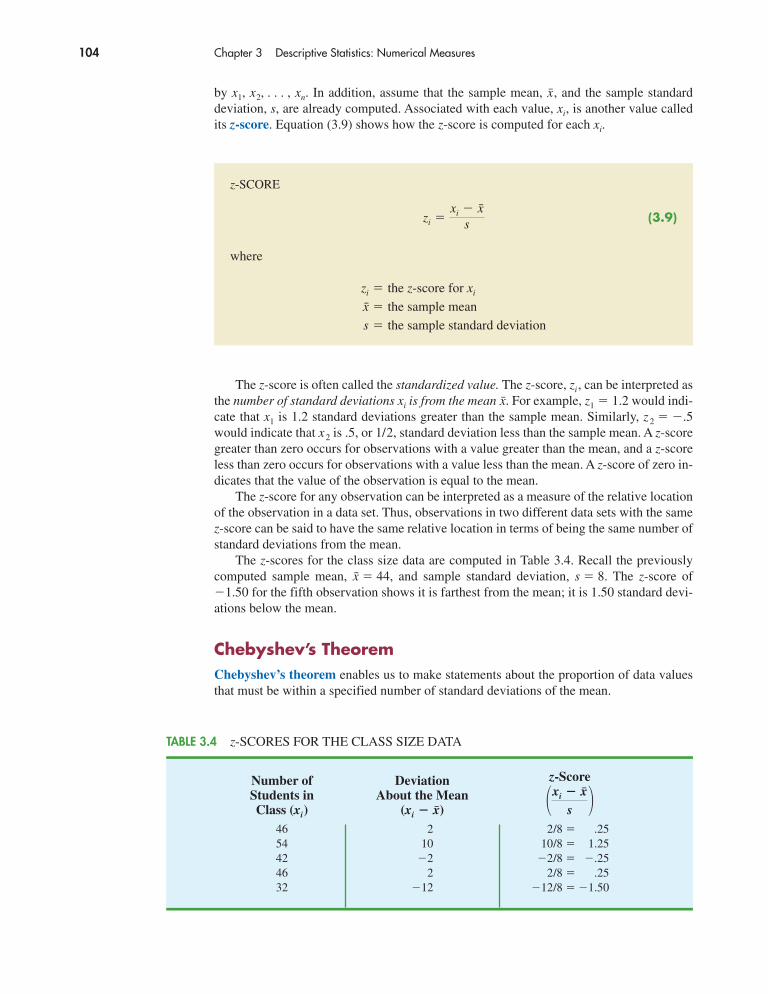
by x1, x2, . . . , xn. In addition, assume that the sample mean, , and the sample standarddeviation, s, are already computed. Associated with each value, xi, is another value calledits z-score. Equation (3.9) shows how the z-score is computed for each xi.
x
The z-score is often called the standardized value. The z-score, zi, can be interpreted asthe number of standard deviations xi is from the mean . For example, z1 � 1.2 would indi-cate that x1 is 1.2 standard deviations greater than the sample mean. Similarly, z 2 � �.5would indicate that x 2 is .5, or 1/2, standard deviation less than the sample mean. A z-scoregreater than zero occurs for observations with a value greater than the mean, and a z-scoreless than zero occurs for observations with a value less than the mean. A z-score of zero in-dicates that the value of the observation is equal to the mean.
The z-score for any observation can be interpreted as a measure of the relative locationof the observation in a data set. Thus, observations in two different data sets with the samez-score can be said to have the same relative location in terms of being the same number ofstandard deviations from the mean.
The z-scores for the class size data are computed in Table 3.4. Recall the previouslycomputed sample mean, � 44, and sample standard deviation, s � 8. The z-score of�1.50 for the fifth observation shows it is farthest from the mean; it is 1.50 standard devi-ations below the mean.
Chebyshev’s TheoremChebyshev’s theorem enables us to make statements about the proportion of data valuesthat must be within a specified number of standard deviations of the mean.
x
x
z-SCORE
(3.9)
where
zi �
x �
s �
the z-score for xi
the sample mean
the sample standard deviation
zi �xi � x
s
Number of Deviation z-Score
46 2 2/8 � .2554 10 10/8 � 1.2542 �2 �2/8 � �.2546 2 2/8 � .2532 �12 �12/8 � �1.50
�xi � xs �About the Mean
(xi � x)Students inClass (xi)
TABLE 3.4 z-SCORES FOR THE CLASS SIZE DATA

3.3 Measures of Distribution Shape, Relative Location, and Detecting Outliers 105
CHEBYSHEV’S THEOREM
At least (1 � 1/z 2) of the data values must be within z standard deviations of the mean,where z is any value greater than 1.
Some of the implications of this theorem, with z � 2, 3, and 4 standard deviations, follow.
• At least .75, or 75%, of the data values must be within z � 2 standard deviationsof the mean.
• At least .89, or 89%, of the data values must be within z � 3 standard deviationsof the mean.
• At least .94, or 94%, of the data values must be within z � 4 standard deviationsof the mean.
For an example using Chebyshev’s theorem, suppose that the midterm test scores for100 students in a college business statistics course had a mean of 70 and a standard devia-tion of 5. How many students had test scores between 60 and 80? How many students hadtest scores between 58 and 82?
For the test scores between 60 and 80, we note that 60 is two standard deviations belowthe mean and 80 is two standard deviations above the mean. Using Chebyshev’s theorem,we see that at least .75, or at least 75%, of the observations must have values within twostandard deviations of the mean. Thus, at least 75% of the students must have scoredbetween 60 and 80.
For the test scores between 58 and 82, we see that (58 � 70)/5 � �2.4 indicates 58 is2.4 standard deviations below the mean and that (82 � 70)/5 � �2.4 indicates 82 is 2.4standard deviations above the mean. Applying Chebyshev’s theorem with z � 2.4, we have
At least 82.6% of the students must have test scores between 58 and 82.
Empirical RuleOne of the advantages of Chebyshev’s theorem is that it applies to any data set regardless ofthe shape of the distribution of the data. Indeed, it could be used with any of the distributionsin Figure 3.3. In many practical applications, however, data sets exhibit a symmetric mound-shaped or bell-shaped distribution like the one shown in Figure 3.4. When the data are believedto approximate this distribution, the empirical rule can be used to determine the percentage ofdata values that must be within a specified number of standard deviations of the mean.
�1 �1
z 2� � �1 �
1
(2.4)2� � .826
EMPIRICAL RULE
For data having a bell-shaped distribution:
• Approximately 68% of the data values will be within one standard deviationof the mean.
• Approximately 95% of the data values will be within two standard deviationsof the mean.
• Almost all of the data values will be within three standard deviations of the mean.
Chebyshev’s theoremrequires z � 1; but z neednot be an integer.
The empirical rule is basedon the normal probabilitydistribution, which will bediscussed in Chapter 6. The normal distribution is used extensivelythroughout the text.

106 Chapter 3 Descriptive Statistics: Numerical Measures
For example, liquid detergent cartons are filled automatically on a production line. Fillingweights frequently have a bell-shaped distribution. If the mean filling weight is 16 ounces and thestandard deviation is .25 ounces, we can use the empirical rule to draw the following conclusions.
• Approximately 68% of the filled cartons will have weights between 15.75 and 16.25 ounces (within one standard deviation of the mean).
• Approximately 95% of the filled cartons will have weights between 15.50 and 16.50 ounces (within two standard deviations of the mean).
• Almost all filled cartons will have weights between 15.25 and 16.75 ounces (withinthree standard deviations of the mean).
Detecting OutliersSometimes a data set will have one or more observations with unusually large or unusuallysmall values. These extreme values are called outliers. Experienced statisticians take stepsto identify outliers and then review each one carefully. An outlier may be a data value thathas been incorrectly recorded. If so, it can be corrected before further analysis. An outliermay also be from an observation that was incorrectly included in the data set; if so, it canbe removed. Finally, an outlier may be an unusual data value that has been recorded cor-rectly and belongs in the data set. In such cases it should remain.
Standardized values (z-scores) can be used to identify outliers. Recall that the empiri-cal rule allows us to conclude that for data with a bell-shaped distribution, almost all thedata values will be within three standard deviations of the mean. Hence, in using z-scoresto identify outliers, we recommend treating any data value with a z-score less than �3 orgreater than �3 as an outlier. Such data values can then be reviewed for accuracy and todetermine whether they belong in the data set.
Refer to the z-scores for the class size data in Table 3.4. The z-score of �1.50 showsthe fifth class size is farthest from the mean. However, this standardized value is well withinthe �3 to �3 guideline for outliers. Thus, the z-scores do not indicate that outliers are pres-ent in the class size data.
FIGURE 3.4 A SYMMETRIC MOUND-SHAPED OR BELL-SHAPED DISTRIBUTION
NOTES AND COMMENTS
1. Chebyshev’s theorem is applicable for any dataset and can be used to state the minimum num-ber of data values that will be within a certain
number of standard deviations of the mean. Ifthe data are known to be approximately bell-shaped, more can be said. For instance, the
It is a good idea to checkfor outliers before makingdecisions based on dataanalysis. Errors are oftenmade in recording data and entering data into thecomputer. Outliers shouldnot necessarily be deleted,but their accuracy andappropriateness should be verified.

3.3 Measures of Distribution Shape, Relative Location, and Detecting Outliers 107
Exercises
Methods25. Consider a sample with data values of 10, 20, 12, 17, and 16. Compute the z-score for each
of the five observations.
26. Consider a sample with a mean of 500 and a standard deviation of 100. What are the z-scores for the following data values: 520, 650, 500, 450, and 280?
27. Consider a sample with a mean of 30 and a standard deviation of 5. Use Chebyshev’s the-orem to determine the percentage of the data within each of the following ranges:a. 20 to 40b. 15 to 45c. 22 to 38d. 18 to 42e. 12 to 48
28. Suppose the data have a bell-shaped distribution with a mean of 30 and a standard devia-tion of 5. Use the empirical rule to determine the percentage of data within each of the fol-lowing ranges:a. 20 to 40b. 15 to 45c. 25 to 35
Applications29. The results of a national survey showed that on average, adults sleep 6.9 hours per night.
Suppose that the standard deviation is 1.2 hours.a. Use Chebyshev’s theorem to calculate the percentage of individuals who sleep be-
tween 4.5 and 9.3 hours.b. Use Chebyshev’s theorem to calculate the percentage of individuals who sleep be-
tween 3.9 and 9.9 hours.c. Assume that the number of hours of sleep follows a bell-shaped distribution. Use the
empirical rule to calculate the percentage of individuals who sleep between 4.5 and9.3 hours per day. How does this result compare to the value that you obtained usingChebyshev’s theorem in part (a)?
30. The Energy Information Administration reported that the mean retail price per gallon ofregular grade gasoline was $2.05 (Energy Information Administration, May 2009).Suppose that the standard deviation was $.10 and that the retail price per gallon has a bell-shaped distribution.a. What percentage of regular grade gasoline sold between $1.95 and $2.15 per gallon?b. What percentage of regular grade gasoline sold between $1.95 and $2.25 per gallon?c. What percentage of regular grade gasoline sold for more than $2.25 per gallon?
31. The national average for the math portion of the College Board’s Scholastic Aptitude Test(SAT) is 515 (The World Almanac, 2009). The College Board periodically rescales the testscores such that the standard deviation is approximately 100. Answer the following ques-tions using a bell-shaped distribution and the empirical rule for the verbal test scores.
empirical rule allows us to say that approxi-mately 95% of the data values will be within twostandard deviations of the mean; Chebyshev’stheorem allows us to conclude only that at least75% of the data values will be in that interval.
2. Before analyzing a data set, statisticians usuallymake a variety of checks to ensure the validity
of data. In a large study it is not uncommon forerrors to be made in recording data values or inentering the values into a computer. Identifyingoutliers is one tool used to check the validity ofthe data.
testSELF
testSELF

108 Chapter 3 Descriptive Statistics: Numerical Measures
a. What percentage of students have an SAT verbal score greater than 615?b. What percentage of students have an SAT verbal score greater than 715?c. What percentage of students have an SAT verbal score between 415 and 515?d. What percentage of students have an SAT verbal score between 315 and 615?
32. The high costs in the California real estate market have caused families who cannot afford tobuy bigger homes to consider backyard sheds as an alternative form of housing expansion.Many are using the backyard structures for home offices, art studios, and hobby areas as wellas for additional storage. The mean price of a customized wooden, shingled backyard struc-ture is $3100 (Newsweek, September 29, 2003). Assume that the standard deviation is $1200.a. What is the z-score for a backyard structure costing $2300?b. What is the z-score for a backyard structure costing $4900?c. Interpret the z-scores in parts (a) and (b). Comment on whether either should be con-
sidered an outlier.d. The Newsweek article described a backyard shed-office combination built in Albany,
California, for $13,000. Should this structure be considered an outlier? Explain.
33. Florida Power & Light (FP&L) Company has enjoyed a reputation for quickly fixing itselectric system after storms. However, during the hurricane seasons of 2004 and 2005, anew reality was that the company’s historical approach to emergency electric systemrepairs was no longer good enough (The Wall Street Journal, January 16, 2006). Datashowing the days required to restore electric service after seven hurricanes during 2004and 2005 follow.
Hurricane Days to Restore Service
Charley 13Frances 12Jeanne 8Dennis 3Katrina 8Rita 2Wilma 18
Based on this sample of seven, compute the following descriptive statistics:a. Mean, median, and modeb. Range and standard deviationc. Should Wilma be considered an outlier in terms of the days required to restore elec-
tric service?d. The seven hurricanes resulted in 10 million service interruptions to customers. Do the
statistics show that FP&L should consider updating its approach to emergency elec-tric system repairs? Discuss.
34. A sample of 10 NCAA college basketball game scores provided the following data (USAToday, January 26, 2004).
WinningWinning Team Points Losing Team Points Margin
Arizona 90 Oregon 66 24Duke 85 Georgetown 66 19Florida State 75 Wake Forest 70 5Kansas 78 Colorado 57 21Kentucky 71 Notre Dame 63 8Louisville 65 Tennessee 62 3Oklahoma State 72 Texas 66 6
fileWEBNCAA
3.4 Exploratory Data Analysis 109
a. Compute the mean and standard deviation for the points scored by the winning team.b. Assume that the points scored by the winning teams for all NCAA games follow a
bell-shaped distribution. Using the mean and standard deviation found in part (a),estimate the percentage of all NCAA games in which the winning team scores 84 ormore points. Estimate the percentage of NCAA games in which the winning teamscores more than 90 points.
c. Compute the mean and standard deviation for the winning margin. Do the data con-tain outliers? Explain.
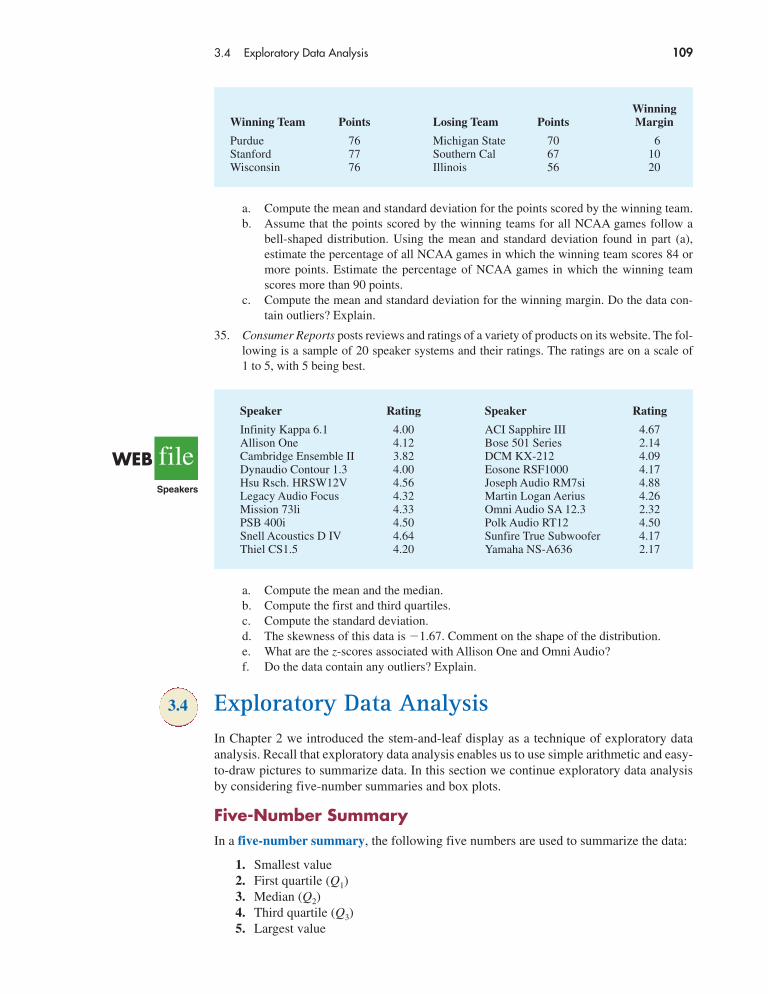
35. Consumer Reports posts reviews and ratings of a variety of products on its website. The fol-lowing is a sample of 20 speaker systems and their ratings. The ratings are on a scale of1 to 5, with 5 being best.
Speaker Rating Speaker Rating
Infinity Kappa 6.1 4.00 ACI Sapphire III 4.67Allison One 4.12 Bose 501 Series 2.14Cambridge Ensemble II 3.82 DCM KX-212 4.09Dynaudio Contour 1.3 4.00 Eosone RSF1000 4.17Hsu Rsch. HRSW12V 4.56 Joseph Audio RM7si 4.88Legacy Audio Focus 4.32 Martin Logan Aerius 4.26Mission 73li 4.33 Omni Audio SA 12.3 2.32PSB 400i 4.50 Polk Audio RT12 4.50Snell Acoustics D IV 4.64 Sunfire True Subwoofer 4.17Thiel CS1.5 4.20 Yamaha NS-A636 2.17
a. Compute the mean and the median.b. Compute the first and third quartiles.c. Compute the standard deviation.d. The skewness of this data is �1.67. Comment on the shape of the distribution.e. What are the z-scores associated with Allison One and Omni Audio?f. Do the data contain any outliers? Explain.
3.4 Exploratory Data AnalysisIn Chapter 2 we introduced the stem-and-leaf display as a technique of exploratory dataanalysis. Recall that exploratory data analysis enables us to use simple arithmetic and easy-to-draw pictures to summarize data. In this section we continue exploratory data analysisby considering five-number summaries and box plots.
Five-Number SummaryIn a five-number summary, the following five numbers are used to summarize the data:
1. Smallest value2. First quartile (Q1)3. Median (Q2)4. Third quartile (Q3)5. Largest value
WinningWinning Team Points Losing Team Points Margin
Purdue 76 Michigan State 70 6Stanford 77 Southern Cal 67 10Wisconsin 76 Illinois 56 20
fileWEBSpeakers
110 Chapter 3 Descriptive Statistics: Numerical Measures
The easiest way to develop a five-number summary is to first place the data in ascend-ing order. Then it is easy to identify the smallest value, the three quartiles, and the largestvalue. The monthly starting salaries shown in Table 3.1 for a sample of 12 business schoolgraduates are repeated here in ascending order.
3310 3355 3450 3480 3480 3490 3520 3540 3550 3650 3730 3925
The median of 3505 and the quartiles Q1 � 3465 and Q3 � 3600 were computed in Sec-tion 3.1. Reviewing the data shows a smallest value of 3310 and a largest value of 3925.Thus the five-number summary for the salary data is 3310, 3465, 3505, 3600, 3925. Ap-proximately one-fourth, or 25%, of the observations are between adjacent numbers in afive-number summary.
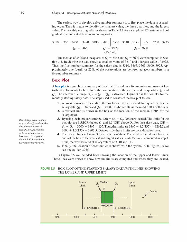
Box PlotA box plot is a graphical summary of data that is based on a five-number summary. A keyto the development of a box plot is the computation of the median and the quartiles, Q1 andQ3. The interquartile range, IQR � Q3 � Q1, is also used. Figure 3.5 is the box plot for themonthly starting salary data. The steps used to construct the box plot follow.
1. Abox is drawn with the ends of the box located at the first and third quartiles. For thesalary data, Q1 � 3465 and Q3 � 3600.This box contains the middle 50% of the data.
2. A vertical line is drawn in the box at the location of the median (3505 for the salary data).
3. By using the interquartile range, IQR � Q3 � Q1, limits are located. The limits for thebox plot are 1.5(IQR) below Q1 and 1.5(IQR) above Q3. For the salary data, IQR �Q3 � Q1 � 3600 � 3465 � 135. Thus, the limits are 3465 � 1.5(135) � 3262.5 and3600 � 1.5(135) � 3802.5. Data outside these limits are considered outliers.
4. The dashed lines in Figure 3.5 are called whiskers. The whiskers are drawn from theends of the box to the smallest and largest values inside the limits computed in step 3.Thus, the whiskers end at salary values of 3310 and 3730.
5. Finally, the location of each outlier is shown with the symbol *. In Figure 3.5 wesee one outlier, 3925.
In Figure 3.5 we included lines showing the location of the upper and lower limits.These lines were drawn to show how the limits are computed and where they are located.
(Median)Q3 � 3600Q2 � 3505Q1 � 3465
���
IQR1.5(IQR) 1.5(IQR)
3200 34003000 3600 3800 4000
Q1 Q3Median Upper
LimitLowerLimit
*
Outlier
FIGURE 3.5 BOX PLOT OF THE STARTING SALARY DATA WITH LINES SHOWING THE LOWER AND UPPER LIMITS
Box plots provide anotherway to identify outliers. Butthey do not necessarilyidentify the same values as those with a z-score less than �3 or greaterthan �3. Either or bothprocedures may be used.

3.4 Exploratory Data Analysis 111
*
3200 34003000 3600 3800 4000
FIGURE 3.6 BOX PLOT OF MONTHLY STARTING SALARY DATA
Although the limits are always computed, generally they are not drawn on the box plots.Figure 3.6 shows the usual appearance of a box plot for the salary data.
In order to compare monthly starting salaries for business school graduates by major, asample of 111 recent graduates was selected. The major and the monthly starting salarywere recorded for each graduate. Figure 3.7 shows the Minitab box plots for accounting, fi-nance, information systems, management, and marketing majors. Note that the major isshown on the horizontal axis and each box plot is shown vertically above the correspond-ing major. Displaying box plots in this manner is an excellent graphical technique for mak-ing comparisons among two or more groups.
What observations can you make about monthly starting salaries by major using the boxplots in Figured 3.7? Specifically, we note the following:
• The higher salaries are in accounting; the lower salaries are in management and marketing.
• Based on the medians, accounting and information systems have similar and highermedian salaries. Finance is next with management and marketing showing lowermedian salaries.
• High salary outliers exist for accounting, finance, and marketing majors.• Finance salaries appear to have the least variation, while accounting salaries appear
to have the most variation.
Perhaps you can see additional interpretations based on these box plots.
fileWEB
MajorSalary
2000
3000
4000
5000
6000
Accounting Finance Info Systems Management Marketing
Business Major
Mon
thly
Sta
rtin
g Sa
lary
FIGURE 3.7 MINITAB BOX PLOTS OF MONTLY STARTING SALARY BY MAJOR
112 Chapter 3 Descriptive Statistics: Numerical Measures
Exercises
Methods36. Consider a sample with data values of 27, 25, 20, 15, 30, 34, 28, and 25. Provide the five-
number summary for the data.
37. Show the box plot for the data in exercise 36.
38. Show the five-number summary and the box plot for the following data: 5, 15, 18, 10, 8,12, 16, 10, 6.
39. A data set has a first quartile of 42 and a third quartile of 50. Compute the lower and upperlimits for the corresponding box plot. Should a data value of 65 be considered an outlier?
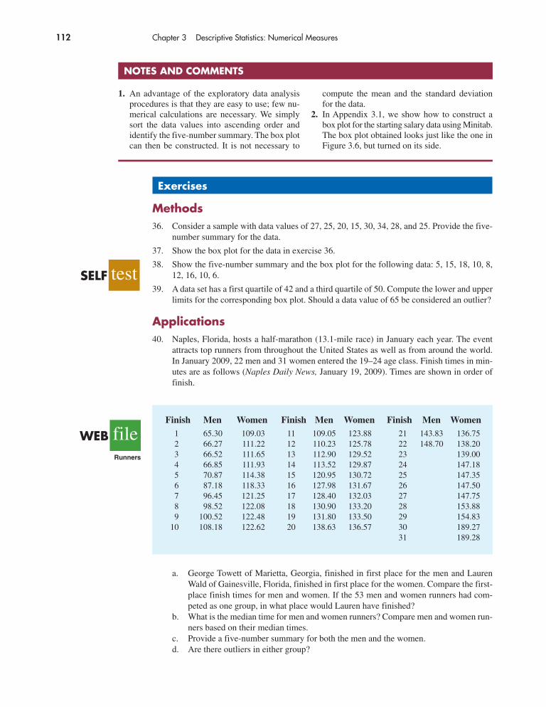
Applications40. Naples, Florida, hosts a half-marathon (13.1-mile race) in January each year. The event
attracts top runners from throughout the United States as well as from around the world.In January 2009, 22 men and 31 women entered the 19–24 age class. Finish times in min-utes are as follows (Naples Daily News, January 19, 2009). Times are shown in order offinish.
NOTES AND COMMENTS
1. An advantage of the exploratory data analysisprocedures is that they are easy to use; few nu-merical calculations are necessary. We simplysort the data values into ascending order andidentify the five-number summary. The box plotcan then be constructed. It is not necessary to
compute the mean and the standard deviationfor the data.
2. In Appendix 3.1, we show how to construct abox plot for the starting salary data using Minitab.The box plot obtained looks just like the one inFigure 3.6, but turned on its side.
testSELF
Finish Men Women Finish Men Women Finish Men Women1 65.30 109.03 11 109.05 123.88 21 143.83 136.752 66.27 111.22 12 110.23 125.78 22 148.70 138.203 66.52 111.65 13 112.90 129.52 23 139.004 66.85 111.93 14 113.52 129.87 24 147.185 70.87 114.38 15 120.95 130.72 25 147.356 87.18 118.33 16 127.98 131.67 26 147.507 96.45 121.25 17 128.40 132.03 27 147.758 98.52 122.08 18 130.90 133.20 28 153.889 100.52 122.48 19 131.80 133.50 29 154.83
10 108.18 122.62 20 138.63 136.57 30 189.2731 189.28
fileWEBRunners
a. George Towett of Marietta, Georgia, finished in first place for the men and LaurenWald of Gainesville, Florida, finished in first place for the women. Compare the first-place finish times for men and women. If the 53 men and women runners had com-peted as one group, in what place would Lauren have finished?
b. What is the median time for men and women runners? Compare men and women run-ners based on their median times.
c. Provide a five-number summary for both the men and the women.d. Are there outliers in either group?

3.4 Exploratory Data Analysis 113
Metropolitan Area AT&T Sprint T-Mobile VerizonAtlanta 70 66 71 79Boston 69 64 74 76Chicago 71 65 70 77Dallas 75 65 74 78Denver 71 67 73 77Detroit 73 65 77 79Jacksonville 73 64 75 81Las Vegas 72 68 74 81Los Angeles 66 65 68 78Miami 68 69 73 80Minneapolis 68 66 75 77Philadelphia 72 66 71 78Phoenix 68 66 76 81San Antonio 75 65 75 80San Diego 69 68 72 79San Francisco 66 69 73 75Seattle 68 67 74 77St. Louis 74 66 74 79Tampa 73 63 73 79Washington 72 68 71 76
fileWEBCellService
e. Show the box plots for the two groups. Did men or women have the most variation infinish times? Explain.
41. Annual sales, in millions of dollars, for 21 pharmaceutical companies follow.
8408 1374 1872 8879 2459 11413608 14138 6452 1850 2818 1356
10498 7478 4019 4341 739 21273653 5794 8305
a. Provide a five-number summary.b. Compute the lower and upper limits.c. Do the data contain any outliers?d. Johnson & Johnson’s sales are the largest on the list at $14,138 million. Suppose a data
entry error (a transposition) had been made and the sales had been entered as $41,138million. Would the method of detecting outliers in part (c) identify this problem andallow for correction of the data entry error?
e. Show a box plot.
42. Consumer Reports provided overall customer satisfaction scores for AT&T, Sprint, T-Mobile, and Verizon cell-phone services in major metropolitan areas throughout theUnited States. The rating for each service reflects the overall customer satisfaction considering a variety of factors such as cost, connectivity problems, dropped calls, staticinterference, and customer support. A satisfaction scale from 0 to 100 was used with 0 in-dicating completely dissatisfied and 100 indicating completely satisfied. The ratings forthe four cell-phone services in 20 metropolitan areas are as shown (Consumer Reports,January 2009).
testSELF
a. Consider T-Mobile first. What is the median rating?b. Develop a five-number summary for the T-Mobile service.c. Are there outliers for T-Mobile? Explain.d. Repeat parts (b) and (c) for the other three cell-phone services.
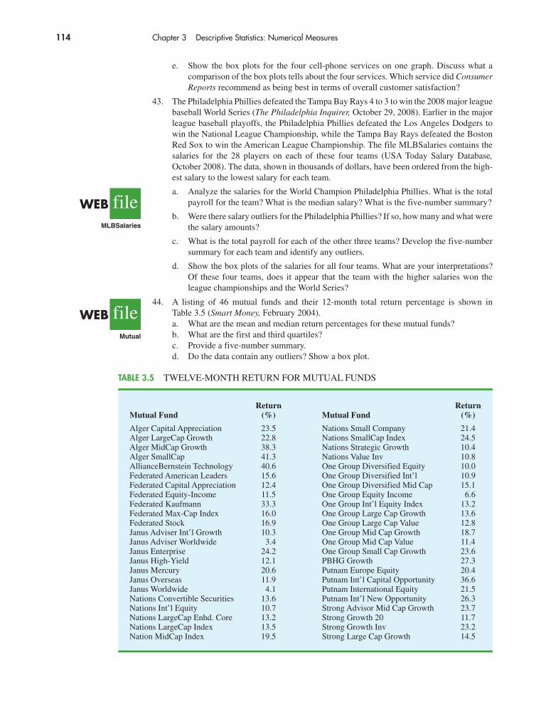
Return ReturnMutual Fund (%) Mutual Fund (%)
Alger Capital Appreciation 23.5 Nations Small Company 21.4Alger LargeCap Growth 22.8 Nations SmallCap Index 24.5Alger MidCap Growth 38.3 Nations Strategic Growth 10.4Alger SmallCap 41.3 Nations Value Inv 10.8AllianceBernstein Technology 40.6 One Group Diversified Equity 10.0Federated American Leaders 15.6 One Group Diversified Int’l 10.9Federated Capital Appreciation 12.4 One Group Diversified Mid Cap 15.1Federated Equity-Income 11.5 One Group Equity Income 6.6Federated Kaufmann 33.3 One Group Int’l Equity Index 13.2Federated Max-Cap Index 16.0 One Group Large Cap Growth 13.6Federated Stock 16.9 One Group Large Cap Value 12.8Janus Adviser Int’l Growth 10.3 One Group Mid Cap Growth 18.7Janus Adviser Worldwide 3.4 One Group Mid Cap Value 11.4Janus Enterprise 24.2 One Group Small Cap Growth 23.6Janus High-Yield 12.1 PBHG Growth 27.3Janus Mercury 20.6 Putnam Europe Equity 20.4Janus Overseas 11.9 Putnam Int’l Capital Opportunity 36.6Janus Worldwide 4.1 Putnam International Equity 21.5Nations Convertible Securities 13.6 Putnam Int’l New Opportunity 26.3Nations Int’l Equity 10.7 Strong Advisor Mid Cap Growth 23.7Nations LargeCap Enhd. Core 13.2 Strong Growth 20 11.7Nations LargeCap Index 13.5 Strong Growth Inv 23.2Nation MidCap Index 19.5 Strong Large Cap Growth 14.5
TABLE 3.5 TWELVE-MONTH RETURN FOR MUTUAL FUNDS
114 Chapter 3 Descriptive Statistics: Numerical Measures
e. Show the box plots for the four cell-phone services on one graph. Discuss what acomparison of the box plots tells about the four services. Which service did ConsumerReports recommend as being best in terms of overall customer satisfaction?
43. The Philadelphia Phillies defeated the Tampa Bay Rays 4 to 3 to win the 2008 major leaguebaseball World Series (The Philadelphia Inquirer, October 29, 2008). Earlier in the majorleague baseball playoffs, the Philadelphia Phillies defeated the Los Angeles Dodgers towin the National League Championship, while the Tampa Bay Rays defeated the BostonRed Sox to win the American League Championship. The file MLBSalaries contains thesalaries for the 28 players on each of these four teams (USA Today Salary Database,October 2008). The data, shown in thousands of dollars, have been ordered from the high-est salary to the lowest salary for each team.
a. Analyze the salaries for the World Champion Philadelphia Phillies. What is the totalpayroll for the team? What is the median salary? What is the five-number summary?
b. Were there salary outliers for the Philadelphia Phillies? If so, how many and what werethe salary amounts?
c. What is the total payroll for each of the other three teams? Develop the five-numbersummary for each team and identify any outliers.
d. Show the box plots of the salaries for all four teams. What are your interpretations?Of these four teams, does it appear that the team with the higher salaries won theleague championships and the World Series?
44. A listing of 46 mutual funds and their 12-month total return percentage is shown in Table 3.5 (Smart Money, February 2004).a. What are the mean and median return percentages for these mutual funds?b. What are the first and third quartiles?c. Provide a five-number summary.d. Do the data contain any outliers? Show a box plot.
fileWEBMutual
fileWEBMLBSalaries

3.5 Measures of Association Between Two Variables 115
3.5 Measures of Association Between Two VariablesThus far we have examined numerical methods used to summarize the data for one variableat a time. Often a manager or decision maker is interested in the relationship between twovariables. In this section we present covariance and correlation as descriptive measures ofthe relationship between two variables.
We begin by reconsidering the application concerning a stereo and sound equipmentstore in San Francisco as presented in Section 2.4. The store’s manager wants to determinethe relationship between the number of weekend television commercials shown and thesales at the store during the following week. Sample data with sales expressed in hundredsof dollars are provided in Table 3.6. It shows 10 observations (n � 10), one for each week.The scatter diagram in Figure 3.8 shows a positive relationship, with higher sales (y) asso-ciated with a greater number of commercials (x). In fact, the scatter diagram suggests thata straight line could be used as an approximation of the relationship. In the following dis-cussion, we introduce covariance as a descriptive measure of the linear association betweentwo variables.
CovarianceFor a sample of size n with the observations (x1, y1), (x2, y2), and so on, the sample covari-ance is defined as follows:
Number of Commercials Sales Volume ($100s)Week x y
1 2 502 5 573 1 414 3 545 4 546 1 387 5 638 3 489 4 59
10 2 46
TABLE 3.6 SAMPLE DATA FOR THE STEREO AND SOUND EQUIPMENT STORE
SAMPLE COVARIANCE
(3.10)sxy ��(xi � x)(
yi � y)
n � 1
This formula pairs each xi with a yi. We then sum the products obtained by multiplying thedeviation of each xi from its sample mean by the deviation of the corresponding yi fromits sample mean ; this sum is then divided by n � 1.y
x
fileWEBStereo

116 Chapter 3 Descriptive Statistics: Numerical Measures
To measure the strength of the linear relationship between the number of commercialsx and the sales volume y in the stereo and sound equipment store problem, we use equa-tion (3.10) to compute the sample covariance. The calculations in Table 3.7 show thecomputation of �(xi � )(yi � ). Note that � 30/10 � 3 and � 510/10 � 51. Usingequation (3.10), we obtain a sample covariance of
sxy ��(xi � x)(yi � y)
n � 1�
99
9� 11
yxyx
35
40
45
50
55
60
65
0 1 2 3 4 5
Number of Commercials
x
y
Sale
s ($
100s
)
FIGURE 3.8 SCATTER DIAGRAM FOR THE STEREO AND SOUND EQUIPMENT STORE
xi yi ( )( )
2 50 �1 �1 15 57 2 6 121 41 �2 �10 203 54 0 3 04 54 1 3 31 38 �2 �13 265 63 2 12 243 48 0 �3 04 59 1 8 82 46 �1 �5 5
Totals 30 510 0 0 99
sx y ��(xi � x)(
yi � y)
n � 1�
99
10 � 1� 11
yi � yxi � xyi � yxi � x
TABLE 3.7 CALCULATIONS FOR THE SAMPLE COVARIANCE
3.5 Measures of Association Between Two Variables 117
In equation (3.11) we use the notation μx for the population mean of the variable x and μy
for the population mean of the variable y. The population covariance σxy is defined for apopulation of size N.
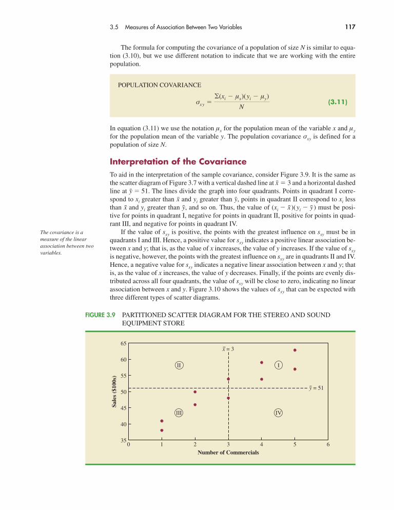
Interpretation of the CovarianceTo aid in the interpretation of the sample covariance, consider Figure 3.9. It is the same asthe scatter diagram of Figure 3.7 with a vertical dashed line at � 3 and a horizontal dashedline at � 51. The lines divide the graph into four quadrants. Points in quadrant I corre-spond to xi greater than and yi greater than , points in quadrant II correspond to xi lessthan and yi greater than , and so on. Thus, the value of (xi � )(yi � ) must be posi-tive for points in quadrant I, negative for points in quadrant II, positive for points in quad-rant III, and negative for points in quadrant IV.
If the value of sxy is positive, the points with the greatest influence on sxy must be inquadrants I and III. Hence, a positive value for sxy indicates a positive linear association be-tween x and y; that is, as the value of x increases, the value of y increases. If the value of sxy
is negative, however, the points with the greatest influence on sxy are in quadrants II and IV.Hence, a negative value for sxy indicates a negative linear association between x and y; thatis, as the value of x increases, the value of y decreases. Finally, if the points are evenly dis-tributed across all four quadrants, the value of sxy will be close to zero, indicating no linearassociation between x and y. Figure 3.10 shows the values of sxy that can be expected withthree different types of scatter diagrams.
yxyxyx
yx
The formula for computing the covariance of a population of size N is similar to equa-tion (3.10), but we use different notation to indicate that we are working with the entirepopulation.
POPULATION COVARIANCE
(3.11)σx y ��(xi � μx)(
yi � μy)
N
65
60
55
50
45
40
35
Sale
s ($
100s
)
0 1 2 3
Number of Commercials4 5 6
II
III
I
IV
x = 3
y = 51
FIGURE 3.9 PARTITIONED SCATTER DIAGRAM FOR THE STEREO AND SOUNDEQUIPMENT STORE
The covariance is ameasure of the linearassociation between twovariables.

118 Chapter 3 Descriptive Statistics: Numerical Measures
y
x
sxy Positive:(x and y are positively
linearly related)
y
x
sxy Approximately 0:(x and y are notlinearly related)
y
x
sxy Negative:(x and y are negatively
linearly related)
FIGURE 3.10 INTERPRETATION OF SAMPLE COVARIANCE

3.5 Measures of Association Between Two Variables 119
Referring again to Figure 3.9, we see that the scatter diagram for the stereo and soundequipment store follows the pattern in the top panel of Figure 3.10. As we should expect,the value of the sample covariance indicates a positive linear relationship with sxy � 11.
From the preceding discussion, it might appear that a large positive value for the co-variance indicates a strong positive linear relationship and that a large negative value indi-cates a strong negative linear relationship. However, one problem with using covariance asa measure of the strength of the linear relationship is that the value of the covariance de-pends on the units of measurement for x and y. For example, suppose we are interested inthe relationship between height x and weight y for individuals. Clearly the strength of therelationship should be the same whether we measure height in feet or inches. Measuringthe height in inches, however, gives us much larger numerical values for (xi � ) thanwhen we measure height in feet. Thus, with height measured in inches, we would obtain alarger value for the numerator �(xi � )(yi � ) in equation (3.10)—and hence a largercovariance—when in fact the relationship does not change. A measure of the relationshipbetween two variables that is not affected by the units of measurement for x and y is thecorrelation coefficient.
Correlation CoefficientFor sample data, the Pearson product moment correlation coefficient is defined as follows.
yx
x
PEARSON PRODUCT MOMENT CORRELATION COEFFICIENT: SAMPLE DATA
(3.12)
where
rxy �
sxy �
sx �
sy �
sample correlation coefficient
sample covariance
sample standard deviation of x
sample standard deviation of y
rxy �sxy
sx sy
Equation (3.12) shows that the Pearson product moment correlation coefficient forsample data (commonly referred to more simply as the sample correlation coefficient) iscomputed by dividing the sample covariance by the product of the sample standard devia-tion of x and the sample standard deviation of y.
Let us now compute the sample correlation coefficient for the stereo and sound equip-ment store. Using the data in Table 3.7, we can compute the sample standard deviations forthe two variables:
Now, because sxy � 11, the sample correlation coefficient equals
rxy �sxy
sxsy
�11
(1.49)(7.93)� .93
sy � � �(
yi � y)2
n � 1� �566
9� 7.93
sx � � �(xi � x)2
n � 1� �20
9� 1.49
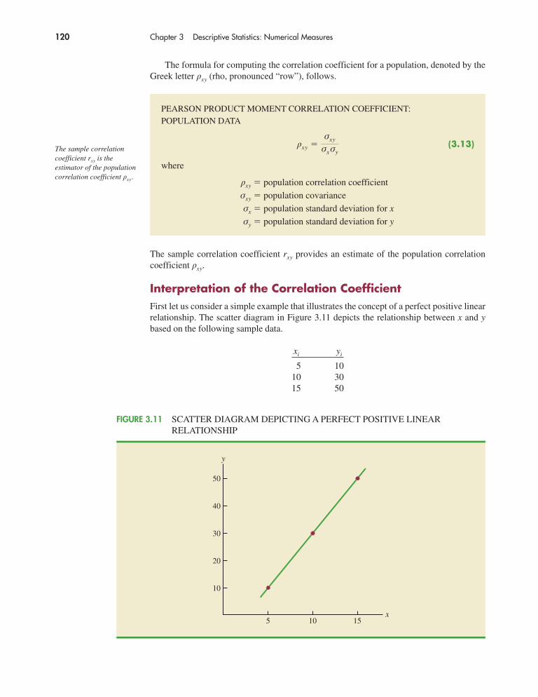
120 Chapter 3 Descriptive Statistics: Numerical Measures
The formula for computing the correlation coefficient for a population, denoted by theGreek letter �xy (rho, pronounced “row”), follows.
PEARSON PRODUCT MOMENT CORRELATION COEFFICIENT: POPULATION DATA
� (3.13)
where
�xy � population correlation coefficient
σxy � population covariance
σx � population standard deviation for x
σy � population standard deviation for y
xy �σxy
σxσyThe sample correlationcoefficient rxy is theestimator of the populationcorrelation coefficient �xy.
The sample correlation coefficient rxy provides an estimate of the population correlationcoefficient �xy.
Interpretation of the Correlation CoefficientFirst let us consider a simple example that illustrates the concept of a perfect positive linearrelationship. The scatter diagram in Figure 3.11 depicts the relationship between x and ybased on the following sample data.
xi yi
5 1010 3015 50
50
40
30
20
10
y
5 10 15x
FIGURE 3.11 SCATTER DIAGRAM DEPICTING A PERFECT POSITIVE LINEARRELATIONSHIP

3.5 Measures of Association Between Two Variables 121
The straight line drawn through each of the three points shows a perfect linear rela-tionship between x and y. In order to apply equation (3.12) to compute the sample correla-tion we must first compute sxy, sx, and sy. Some of the computations are shown in Table 3.8.Using the results in this table, we find
Thus, we see that the value of the sample correlation coefficient is 1.In general, it can be shown that if all the points in a data set fall on a positively sloped
straight line, the value of the sample correlation coefficient is �1; that is, a sample corre-lation coefficient of �1 corresponds to a perfect positive linear relationship between x andy. Moreover, if the points in the data set fall on a straight line having negative slope, thevalue of the sample correlation coefficient is �1; that is, a sample correlation coefficientof �1 corresponds to a perfect negative linear relationship between x and y.
Let us now suppose that a certain data set indicates a positive linear relationship be-tween x and y but that the relationship is not perfect. The value of rxy will be less than 1,indicating that the points in the scatter diagram are not all on a straight line. As the pointsdeviate more and more from a perfect positive linear relationship, the value of rxy becomessmaller and smaller. A value of rxy equal to zero indicates no linear relationship between xand y, and values of rxy near zero indicate a weak linear relationship.
For the data involving the stereo and sound equipment store, rxy � .93. Therefore, weconclude that a strong positive linear relationship occurs between the number of commer-cials and sales. More specifically, an increase in the number of commercials is associatedwith an increase in sales.
In closing, we note that correlation provides a measure of linear association and notnecessarily causation. A high correlation between two variables does not mean thatchanges in one variable will cause changes in the other variable. For example, we mayfind that the quality rating and the typical meal price of restaurants are positively corre-lated. However, simply increasing the meal price at a restaurant will not cause the qualityrating to increase.
rxy �sxy
sx sy
�100
5(20)� 1
sy � � �(
yi � y)2
n � 1� �800
2� 20
sx � � �(xi � x)2
n � 1� �50
2� 5
sxy ��(xi � x)(
yi � y)
n � 1�
200
2� 100
xi yi ( )2 ( )2 ( )( )5 10 �5 25 �20 400 100
10 30 0 0 0 0 015 50 5 25 20 400 100
Totals 30 90 0 50 0 800 200
y � 30x � 10
yi � yxi � xyi � yyi � yxi � xxi � x
TABLE 3.8 COMPUTATIONS USED IN CALCULATING THE SAMPLE CORRELATION COEFFICIENT
The correlation coefficientranges from �1 to �1.Values close to �1 or �1indicate a strong linearrelationship. The closer thecorrelation is to zero, theweaker the relationship.

122 Chapter 3 Descriptive Statistics: Numerical Measures
Exercises
Methods45. Five observations taken for two variables follow.
xi 4 6 11 3 16
yi 50 50 40 60 30
a. Develop a scatter diagram with x on the horizontal axis.b. What does the scatter diagram developed in part (a) indicate about the relationship
between the two variables?c. Compute and interpret the sample covariance.d. Compute and interpret the sample correlation coefficient.
46. Five observations taken for two variables follow.
xi 6 11 15 21 27
yi 6 9 6 17 12
a. Develop a scatter diagram for these data.b. What does the scatter diagram indicate about a relationship between x and y?c. Compute and interpret the sample covariance.d. Compute and interpret the sample correlation coefficient.
Applications47. Nielsen Media Research provides two measures of the television viewing audience: a tele-
vision program rating, which is the percentage of households with televisions watching aprogram, and a television program share, which is the percentage of households watchinga program among those with televisions in use. The following data show the Nielsen tele-vision ratings and share data for the Major League Baseball World Series over a nine-yearperiod (Associated Press, October 27, 2003).
Rating 19 17 17 14 16 12 15 12 13
Share 32 28 29 24 26 20 24 20 22
a. Develop a scatter diagram with rating on the horizontal axis.b. What is the relationship between rating and share? Explain.c. Compute and interpret the sample covariance.d. Compute the sample correlation coefficient. What does this value tell us about the
relationship between rating and share?
48. A department of transportation’s study on driving speed and miles per gallon for midsizeautomobiles resulted in the following data:
Speed (Miles per Hour) 30 50 40 55 30 25 60 25 50 55
Miles per Gallon 28 25 25 23 30 32 21 35 26 25
Compute and interpret the sample correlation coefficient.
49. At the beginning of 2009, the economic downturn resulted in the loss of jobs and an in-crease in delinquent loans for housing. The national unemployment rate was 6.5% and thepercentage of delinquent loans was 6.12% (The Wall Street Journal, January 27, 2009). Inprojecting where the real estate market was headed in the coming year, economists stud-ied the relationship between the jobless rate and the percentage of delinquent loans. The expectation was that if the jobless rate continued to increase, there would also be an
testSELF

3.5 Measures of Association Between Two Variables 123
increase in the percentage of delinquent loans. The data below show the jobless rate andthe delinquent loan percentage for 27 major real estate markets.
a. Compute the correlation coefficient. Is there a positive correlation between the joblessrate and the percentage of delinquent housing loans? What is your interpretation?
b. Show a scatter diagram of the relationship between jobless rate and the percentage ofdelinquent housing loans.
50. The Dow Jones Industrial Average (DJIA) and the Standard & Poor’s 500 Index (S&P 500)are both used to measure the performance of the stock market. The DJIA is based on theprice of stocks for 30 large companies; the S&P 500 is based on the price of stocks for 500companies. If both the DJIA and S&P 500 measure the performance of the stock market,how are they correlated? The following data show the daily percent increase or dailypercent decrease in the DJIA and S&P 500 for a sample of nine days over a three-monthperiod (The Wall Street Journal, January 15 to March 10, 2006).
a. Show a scatter diagram.b. Compute the sample correlation coefficient for these data.c. Discuss the association between the DJIA and S&P 500. Do you need to check both
before having a general idea about the daily stock market performance?
51. The daily high and low temperatures for 14 cities around the world are shown (The WeatherChannel, April 22, 2009).
DJIA .20 .82 �.99 .04 �.24 1.01 .30 .55 �.25S&P 500 .24 .19 �.91 .08 �.33 .87 .36 .83 �.16
City High Low City High Low
Athens 68 50 London 67 45Beijing 70 49 Moscow 44 29Berlin 65 44 Paris 69 44Cairo 96 64 Rio de Janeiro 76 69Dublin 57 46 Rome 69 51Geneva 70 45 Tokyo 70 58Hong Kong 80 73 Toronto 44 39
Jobless Delinquent Jobless DelinquentMetro Area Rate (%) Loan (%) Metro Area Rate (%) Loan (%)
Atlanta 7.1 7.02 New York 6.2 5.78Boston 5.2 5.31 Orange County 6.3 6.08Charlotte 7.8 5.38 Orlando 7.0 10.05Chicago 7.8 5.40 Philadelphia 6.2 4.75Dallas 5.8 5.00 Phoenix 5.5 7.22Denver 5.8 4.07 Portland 6.5 3.79Detroit 9.3 6.53 Raleigh 6.0 3.62Houston 5.7 5.57 Sacramento 8.3 9.24Jacksonville 7.3 6.99 St. Louis 7.5 4.40Las Vegas 7.6 11.12 San Diego 7.1 6.91Los Angeles 8.2 7.56 San Francisco 6.8 5.57Miami 7.1 12.11 Seattle 5.5 3.87Minneapolis 6.3 4.39 Tampa 7.5 8.42Nashville 6.6 4.78
fileWEBHousing
fileWEBStockMarket
fileWEBWorldTemp
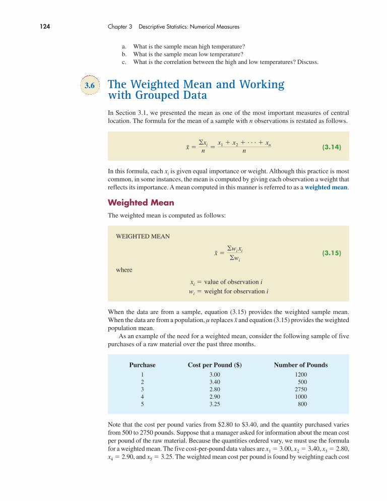
124 Chapter 3 Descriptive Statistics: Numerical Measures
a. What is the sample mean high temperature?b. What is the sample mean low temperature?c. What is the correlation between the high and low temperatures? Discuss.
3.6 The Weighted Mean and Working with Grouped DataIn Section 3.1, we presented the mean as one of the most important measures of centrallocation. The formula for the mean of a sample with n observations is restated as follows.
(3.14)x ��xi
n �x1 � x2 � . . . � xn
n
WEIGHTED MEAN
(3.15)
where
xi �
wi �
value of observation i
weight for observation i
x ��wi
xi
�wi
Purchase Cost per Pound ($) Number of Pounds1 3.00 12002 3.40 5003 2.80 27504 2.90 10005 3.25 800
In this formula, each xi is given equal importance or weight. Although this practice is mostcommon, in some instances, the mean is computed by giving each observation a weight thatreflects its importance. A mean computed in this manner is referred to as a weighted mean.
Weighted MeanThe weighted mean is computed as follows:
When the data are from a sample, equation (3.15) provides the weighted sample mean.When the data are from a population, μ replaces and equation (3.15) provides the weightedpopulation mean.
As an example of the need for a weighted mean, consider the following sample of fivepurchases of a raw material over the past three months.
x
Note that the cost per pound varies from $2.80 to $3.40, and the quantity purchased variesfrom 500 to 2750 pounds. Suppose that a manager asked for information about the mean costper pound of the raw material. Because the quantities ordered vary, we must use the formulafor a weighted mean. The five cost-per-pound data values are x1 � 3.00, x2 � 3.40, x3 � 2.80,x4 � 2.90, and x5 � 3.25. The weighted mean cost per pound is found by weighting each cost

3.6 The Weighted Mean and Working with Grouped Data 125
by its corresponding quantity. For this example, the weights are w1 � 1200, w2 � 500,w3 � 2750, w4 � 1000, and w5 � 800. Based on equation (3.15), the weighted mean iscalculated as follows:
Thus, the weighted mean computation shows that the mean cost per pound for the raw ma-terial is $2.96. Note that using equation (3.14) rather than the weighted mean formula wouldhave provided misleading results. In this case, the mean of the five cost-per-pound valuesis (3.00 � 3.40 � 2.80 � 2.90 � 3.25)/5 � 15.35/5 � $3.07, which overstates the actualmean cost per pound purchased.
The choice of weights for a particular weighted mean computation depends upon the ap-plication. An example that is well known to college students is the computation of a gradepoint average (GPA). In this computation, the data values generally used are 4 for an A grade,3 for a B grade, 2 for a C grade, 1 for a D grade, and 0 for an F grade. The weights are thenumber of credits hours earned for each grade. Exercise 54 at the end of this section pro-vides an example of this weighted mean computation. In other weighted mean computa-tions, quantities such as pounds, dollars, or volume are frequently used as weights. In anycase, when observations vary in importance, the analyst must choose the weight that bestreflects the importance of each observation in the determination of the mean.
Grouped DataIn most cases, measures of location and variability are computed by using the individual datavalues. Sometimes, however, data are available only in a grouped or frequency distributionform. In the following discussion, we show how the weighted mean formula can be used toobtain approximations of the mean, variance, and standard deviation for grouped data.
In Section 2.2 we provided a frequency distribution of the time in days required tocomplete year-end audits for the public accounting firm of Sanderson and Clifford. Thefrequency distribution of audit times is shown in Table 3.9. Based on this frequency distri-bution, what is the sample mean audit time?
To compute the mean using only the grouped data, we treat the midpoint of each class as being representative of the items in the class. Let Mi denote the midpoint for class i and let fi denote the frequency of class i. The weighted mean formula (3.15) is thenused with the data values denoted as Mi and the weights given by the frequencies fi. In this case, the denominator of equation (3.15) is the sum of the frequencies, which is the
�18,500
6250� 2.96
x �1200(3.00) � 500(3.40) � 2750(2.80) � 1000(2.90) � 800(3.25)
1200 � 500 � 2750 � 1000 � 800
Computing a grade pointaverage is a good example ofthe use of a weighted mean.
Audit Time(days) Frequency10–14 415–19 820–24 525–29 230–34 1
Total 20
TABLE 3.9 FREQUENCY DISTRIBUTION OF AUDIT TIMES
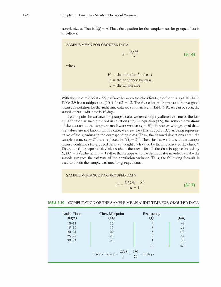
126 Chapter 3 Descriptive Statistics: Numerical Measures
SAMPLE MEAN FOR GROUPED DATA
(3.16)
where
Mi �
fi �
n �
the midpoint for class i
the frequency for class i
the sample size
x �� fi
Mi
n
Audit Time Class Midpoint Frequency(days) (Mi) ( fi) fiMi
10–14 12 4 4815–19 17 8 13620–24 22 5 11025–29 27 2 5430–34 32 1 32
20 380
Sample mean x �� fiMi
n�
380
20� 19 days
TABLE 3.10 COMPUTATION OF THE SAMPLE MEAN AUDIT TIME FOR GROUPED DATA
sample size n. That is, �fi � n. Thus, the equation for the sample mean for grouped data isas follows.
SAMPLE VARIANCE FOR GROUPED DATA
(3.17)s2 �� fi
(Mi � x)2
n � 1
With the class midpoints, Mi, halfway between the class limits, the first class of 10–14 inTable 3.9 has a midpoint at (10 � 14)/2 � 12. The five class midpoints and the weightedmean computation for the audit time data are summarized in Table 3.10. As can be seen, thesample mean audit time is 19 days.
To compute the variance for grouped data, we use a slightly altered version of the for-mula for the variance provided in equation (3.5). In equation (3.5), the squared deviationsof the data about the sample mean were written (xi � )2. However, with grouped data,the values are not known. In this case, we treat the class midpoint, Mi, as being represen-tative of the xi values in the corresponding class. Thus, the squared deviations about thesample mean, (xi � )2, are replaced by (Mi � )2. Then, just as we did with the samplemean calculations for grouped data, we weight each value by the frequency of the class, fi.The sum of the squared deviations about the mean for all the data is approximated by�fi(Mi � )2. The term n � 1 rather than n appears in the denominator in order to make thesample variance the estimate of the population variance. Thus, the following formula isused to obtain the sample variance for grouped data.
x
xx
xx

3.6 The Weighted Mean and Working with Grouped Data 127
Audit Class SquaredTime Midpoint Frequency Deviation Deviation(days) (Mi) ( fi) ( ) ( )2 fi( )2
10–14 12 4 �7 49 19615–19 17 8 �2 4 3220–24 22 5 3 9 4525–29 27 2 8 64 12830–34 32 1 13 169 169
20 570
Sample variance s2 �� fi(Mi � x)2
n � 1�
570
19� 30
� fi(Mi � x)2
Mi � xMi � xMi � x
TABLE 3.11 COMPUTATION OF THE SAMPLE VARIANCE OF AUDIT TIMES FOR GROUPED DATA (SAMPLE MEAN � 19)x
NOTES AND COMMENTS
In computing descriptive statistics for groupeddata, the class midpoints are used to approximatethe data values in each class. As a result, the de-scriptive statistics for grouped data approximatethe descriptive statistics that would result from us-
ing the original data directly. We therefore recom-mend computing descriptive statistics from theoriginal data rather than from grouped data when-ever possible.
POPULATION MEAN FOR GROUPED DATA
(3.18)μ �� fi
Mi
N
POPULATION VARIANCE FOR GROUPED DATA
(3.19)σ 2 �� fi
(Mi � μ)2
N
The calculation of the sample variance for audit times based on the grouped data is shownin Table 3.11. The sample variance is 30.
The standard deviation for grouped data is simply the square root of the variance forgrouped data. For the audit time data, the sample standard deviation is
Before closing this section on computing measures of location and dispersion forgrouped data, we note that formulas (3.16) and (3.17) are for a sample. Population summarymeasures are computed similarly. The grouped data formulas for a population mean andvariance follow.
s � �30 � 5.48.

128 Chapter 3 Descriptive Statistics: Numerical Measures
Exercises
Methods52. Consider the following data and corresponding weights.
xi Weight (wi)
3.2 62.0 32.5 25.0 8
a. Compute the weighted mean.b. Compute the sample mean of the four data values without weighting. Note the differ-
ence in the results provided by the two computations.
53. Consider the sample data in the following frequency distribution.
a. Compute the sample mean.b. Compute the sample variance and sample standard deviation.
Applications54. The grade point average for college students is based on a weighted mean computation.
For most colleges, the grades are given the following data values: A (4), B (3), C (2), D (1), and F (0). After 60 credit hours of course work, a student at State University earned9 credit hours of A, 15 credit hours of B, 33 credit hours of C, and 3 credit hours of D.a. Compute the student’s grade point average.b. Students at State University must maintain a 2.5 grade point average for their first
60 credit hours of course work in order to be admitted to the business college. Will this student be admitted?
55. Morningstar tracks the total return for a large number of mutual funds. The following tableshows the total return and the number of funds for four categories of mutual funds (Morningstar Funds500, 2008).
Class Midpoint Frequency
3–7 5 48–12 10 7
13–17 15 918–22 20 5
testSELF
testSELF
Type of Fund Number of Funds Total Return (%)
Domestic Equity 9191 4.65International Equity 2621 18.15Specialty Stock 1419 11.36Hybrid 2900 6.75
a. Using the number of funds as weights, compute the weighted average total return forthe mutual funds covered by Morningstar.
b. Is there any difficulty associated with using the “number of funds” as the weights incomputing the weighted average total return for Morningstar in part (a)? Discuss. Whatelse might be used for weights?
c. Suppose you had invested $10,000 in mutual funds at the beginning of 2007 anddiversified the investment by placing $2000 in Domestic Equity funds, $4000 in

3.6 The Weighted Mean and Working with Grouped Data 129
Quality Business School CorporateAssessment Deans Recruiters
5 44 314 66 343 60 432 10 121 0 0
International Equity funds, $3000 in Specialty Stock funds, and $1000 in Hybridfunds. What is the expected return on the portfolio?
56. Based on a survey of 425 master’s programs in business administration, the U. S. News &World Report ranked the Indiana University Kelley Business School as the 20th best busi-ness program in the country (America’s Best Graduate Schools, 2009). The ranking wasbased in part on surveys of business school deans and corporate recruiters. Each survey re-spondent was asked to rate the overall academic quality of the master’s program on a scalefrom 1 “marginal” to 5 “outstanding.” Use the sample of responses shown below to computethe weighted mean score for the business school deans and the corporate recruiters. Discuss.
57. The following frequency distribution shows the price per share of the 30 companies in theDow Jones Industrial Average (Barron’s, February 2, 2009).
a. Compute the mean price per share and the standard deviation of the price per share forthe Dow Jones Industrial Average companies.
b. On January 16, 2006, the mean price per share was $45.83 and the standard deviationwas $18.14. Comment on the changes in the price per share over the three-year period.
Summary
In this chapter we introduced several descriptive statistics that can be used to summarize the lo-cation, variability, and shape of a data distribution. Unlike the tabular and graphical proceduresintroduced in Chapter 2, the measures introduced in this chapter summarize the data in terms ofnumerical values. When the numerical values obtained are for a sample, they are called samplestatistics. When the numerical values obtained are for a population, they are called populationparameters. Some of the notation used for sample statistics and population parameters follow.
Price per Number ofShare Companies
$0–9 4$10–19 5$20–29 7$30–39 3$40–49 4$50–59 4$60–69 0$70–79 2$80–89 0$90–99 1
Sample Statistic Population ParameterMean μVarianceStandard deviation s σCovariance s σCorrelation r �x yx y
x yx y
σ 2s2x
In statistical inference, thesample statistic is referredto as the point estimator ofthe population parameter.

130 Chapter 3 Descriptive Statistics: Numerical Measures
As measures of central location, we defined the mean, median, and mode. Then the con-cept of percentiles was used to describe other locations in the data set. Next, we presentedthe range, interquartile range, variance, standard deviation, and coefficient of variation asmeasures of variability or dispersion. Our primary measure of the shape of a data distribu-tion was the skewness. Negative values indicate a data distribution skewed to the left. Posi-tive values indicate a data distribution skewed to the right. We then described how the meanand standard deviation could be used, applying Chebyshev’s theorem and the empiricalrule, to provide more information about the distribution of data and to identify outliers.
In Section 3.4 we showed how to develop a five-number summary and a box plot toprovide simultaneous information about the location, variability, and shape of the dis-tribution. In Section 3.5 we introduced covariance and the correlation coefficient asmeasures of association between two variables. In the final section, we showed how tocompute a weighted mean and how to calculate a mean, variance, and standard deviationfor grouped data.
The descriptive statistics we discussed can be developed using statistical software pack-ages and spreadsheets. In the chapter-ending appendixes we show how to use Minitab, Excel, and StatTools to develop the descriptive statistics introduced in this chapter.
Glossary
Sample statistic A numerical value used as a summary measure for a sample (e.g., thesample mean, , the sample variance, s2, and the sample standard deviation, s).Population parameter A numerical value used as a summary measure for a population(e.g., the population mean, μ, the population variance, σ 2, and the population standard de-viation, σ).Point estimator The sample statistic, such as , s2, and s, when used to estimate the corre-sponding population parameter.Mean A measure of central location computed by summing the data values and dividing bythe number of observations.Median A measure of central location provided by the value in the middle when the dataare arranged in ascending order.Mode A measure of location, defined as the value that occurs with greatest frequency.Percentile A value such that at least p percent of the observations are less than or equal tothis value and at least (100 � p) percent of the observations are greater than or equal to thisvalue. The 50th percentile is the median.Quartiles The 25th, 50th, and 75th percentiles, referred to as the first quartile, the secondquartile (median), and third quartile, respectively. The quartiles can be used to divide a dataset into four parts, with each part containing approximately 25% of the data.Range A measure of variability, defined to be the largest value minus the smallest value.Interquartile range (IQR) A measure of variability, defined to be the difference betweenthe third and first quartiles.Variance A measure of variability based on the squared deviations of the data values aboutthe mean.Standard deviation A measure of variability computed by taking the positive square rootof the variance.Coefficient of variation A measure of relative variability computed by dividing the stan-dard deviation by the mean and multiplying by 100.Skewness A measure of the shape of a data distribution. Data skewed to the left result innegative skewness; a symmetric data distribution results in zero skewness; and data skewedto the right result in positive skewness.
x
x

Key Formulas 131
z-score A value computed by dividing the deviation about the mean (xi � ) by the stan-dard deviation s. A z-score is referred to as a standardized value and denotes the number ofstandard deviations xi is from the mean.Chebyshev’s theorem A theorem that can be used to make statements about the proportionof data values that must be within a specified number of standard deviations of the mean.Empirical rule A rule that can be used to compute the percentage of data values thatmust be within one, two, and three standard deviations of the mean for data that exhibit abell-shaped distribution.Outlier An unusually small or unusually large data value.Five-number summary An exploratory data analysis technique that uses five numbers tosummarize the data: smallest value, first quartile, median, third quartile, and largest value.Box plot A graphical summary of data based on a five-number summary.Covariance A measure of linear association between two variables. Positive values indi-cate a positive relationship; negative values indicate a negative relationship.Correlation coefficient A measure of linear association between two variables that takeson values between �1 and �1. Values near �1 indicate a strong positive linear relation-ship; values near �1 indicate a strong negative linear relationship; and values near zeroindicate the lack of a linear relationship.Weighted mean The mean obtained by assigning each observation a weight that reflects itsimportance.Grouped data Data available in class intervals as summarized by a frequency distribution.Individual values of the original data are not available.
Key Formulas
Sample Mean
(3.1)
Population Mean
(3.2)
Interquartile Range
(3.3)
Population Variance
(3.4)
Sample Variance
(3.5)
Standard Deviation
(3.6)
(3.7)Population standard deviation � σ � �σ 2
Sample standard deviation � s � �s2
s2 ��(xi � x)2
n � 1
σ 2 ��(xi � μ)2
N
IQR � Q3 � Q1
μ ��xi
N
x ��xi
n
x
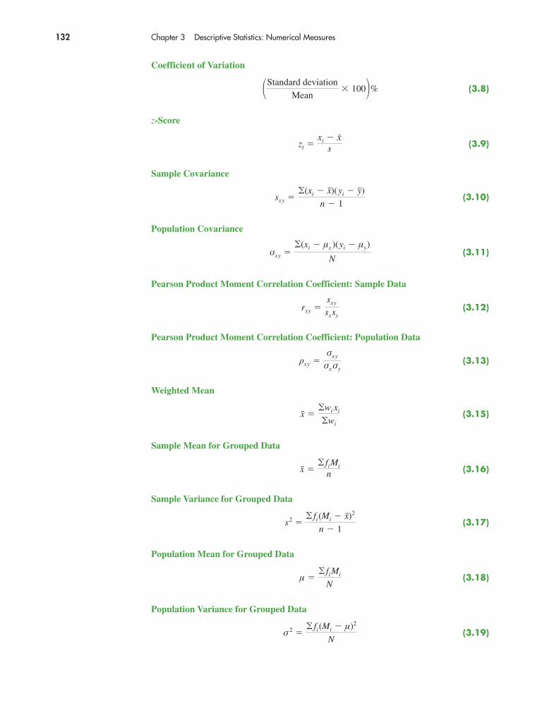
132 Chapter 3 Descriptive Statistics: Numerical Measures
Coefficient of Variation
(3.8)
z-Score
(3.9)
Sample Covariance
(3.10)
Population Covariance
(3.11)
Pearson Product Moment Correlation Coefficient: Sample Data
(3.12)
Pearson Product Moment Correlation Coefficient: Population Data
� (3.13)
Weighted Mean
(3.15)
Sample Mean for Grouped Data
(3.16)
Sample Variance for Grouped Data
(3.17)
Population Mean for Grouped Data
(3.18)
Population Variance for Grouped Data
(3.19)σ 2 �� fi
(Mi � μ)2
N
μ �� fi
Mi
N
s2 �� fi
(Mi � x)2
n � 1
x �� fi
Mi
n
x ��wi xi
�wi
xy �σxy
σxσy
rxy �sxy
sx sy
σxy ��(xi � μx )(
yi � μy)
N
sxy ��(xi � x)(
yi � y)
n � 1
zi �xi � x
s
�Standard deviation
Mean� 100�%

Supplementary Exercises 133
Supplementary Exercises
58. According to an annual consumer spending survey, the average monthly Bank of AmericaVisa credit card charge was $1838 (U.S. Airways Attaché Magazine, December 2003). Asample of monthly credit card charges provides the following data.
236 1710 1351 825 7450316 4135 1333 1584 387991 3396 170 1428 1688
a. Compute the mean and median.b. Compute the first and third quartiles.c. Compute the range and interquartile range.d. Compute the variance and standard deviation.e. The skewness measure for these data is 2.12. Comment on the shape of this distribu-
tion. Is it the shape you would expect? Why or why not?f. Do the data contain outliers?
59. The U.S. Census Bureau provides statistics on family life in the United States, includingthe age at the time of first marriage, current marital status, and size of household (U.S. Census Bureau website, March 20, 2006). The following data show the age at thetime of first marriage for a sample of men and a sample of women.
Men 26 23 28 25 27 30 26 35 2821 24 27 29 30 27 32 27 25
Women 20 28 23 30 24 29 26 2522 22 25 23 27 26 19
a. Determine the median age at the time of first marriage for men and women.b. Compute the first and third quartiles for both men and women.c. Twenty-five years ago the median age at the time of first marriage was 25 for men and
22 for women. What insight does this information provide about the decision of whento marry among young people today?
60. Dividend yield is the annual dividend per share a company pays divided by the currentmarket price per share expressed as a percentage. A sample of 10 large companies providedthe following dividend yield data (The Wall Street Journal, January 16, 2004).
Company Yield % Company Yield %
Altria Group 5.0 General Motors 3.7American Express 0.8 JPMorgan Chase 3.5Caterpillar 1.8 McDonald’s 1.6Eastman Kodak 1.9 United Technology 1.5ExxonMobil 2.5 Wal-Mart Stores 0.7
a. What are the mean and median dividend yields?b. What are the variance and standard deviation?c. Which company provides the highest dividend yield?d. What is the z-score for McDonald’s? Interpret this z-score.e. What is the z-score for General Motors? Interpret this z-score.f. Based on z-scores, do the data contain any outliers?
fileWEBVisa
fileWEBAges

134 Chapter 3 Descriptive Statistics: Numerical Measures
61. The U.S. Department of Education reports that about 50% of all college students use astudent loan to help cover college expenses (National Center for Educational Studies,January 2006). A sample of students who graduated with student loan debt is shown here.The data, in thousands of dollars, show typical amounts of debt upon graduation.
10.1 14.8 5.0 10.2 12.4 12.2 2.0 11.5 17.8 4.0
a. For those students who use a student loan, what is the mean loan debt upon graduation?b. What is the variance? Standard deviation?
62. Small business owners often look to payroll service companies to handle their employeepayroll. Reasons are that small business owners face complicated tax regulations andpenalties for employment tax errors are costly. According to the Internal Revenue Service,26% of all small business employment tax returns contained errors that resulted in a taxpenalty to the owner (The Wall Street Journal, January 30, 2006). The tax penalty for asample of 20 small business owners follows:
820 270 450 1010 890 700 1350 350 300 1200390 730 2040 230 640 350 420 270 370 620
a. What is the mean tax penalty for improperly filed employment tax returns?b. What is the standard deviation?c. Is the highest penalty, $2040, an outlier?d. What are some of the advantages of a small business owner hiring a payroll service
company to handle employee payroll services, including the employment tax returns?
63. Public transportation and the automobile are two methods an employee can use to get to workeach day. Samples of times recorded for each method are shown. Times are in minutes.
Public Transportation: 28 29 32 37 33 25 29 32 41 34Automobile: 29 31 33 32 34 30 31 32 35 33
a. Compute the sample mean time to get to work for each method.b. Compute the sample standard deviation for each method.c. On the basis of your results from parts (a) and (b), which method of transportation
should be preferred? Explain.d. Develop a box plot for each method. Does a comparison of the box plots support your
conclusion in part (c)?
64. The National Association of Realtors reported the median home price in the United Statesand the increase in median home price over a five-year period (The Wall Street Journal, Jan-uary 16, 2006). Use the sample home prices shown here to answer the following questions.
995.9 48.8 175.0 263.5 298.0 218.9 209.0628.3 111.0 212.9 92.6 2325.0 958.0 212.5
a. What is the sample median home price?b. In January 2001, the National Association of Realtors reported a median home price
of $139,300 in the United States. What was the percentage increase in the medianhome price over the five-year period?
c. What are the first quartile and the third quartile for the sample data?d. Provide a five-number summary for the home prices.e. Do the data contain any outliers?f. What is the mean home price for the sample? Why does the National Association of
Realtors prefer to use the median home price in its reports?
65. The U.S. Census Bureau’s American Community Survey reported the percentage ofchildren under 18 years of age who had lived below the poverty level during the previous12 months (U.S. Census Bureau website, August 2008). The region of the country, North-east (NE), Southeast (SE), Midwest (MW), Southwest (SW), and West (W) and the per-centage of children under 18 who had lived below the poverty level are shown for each state.
fileWEBPenalty
fileWEBHomes

Supplementary Exercises 135
fileWEBPovertyLevel
State Region Poverty % State Region Poverty %
Alabama SE 23.0 Montana W 17.3Alaska W 15.1 Nebraska MW 14.4Arizona SW 19.5 Nevada W 13.9Arkansas SE 24.3 New Hampshire NE 9.6California W 18.1 New Jersey NE 11.8Colorado W 15.7 New Mexico SW 25.6Connecticut NE 11.0 New York NE 20.0Delaware NE 15.8 North Carolina SE 20.2Florida SE 17.5 North Dakota MW 13.0Georgia SE 20.2 Ohio MW 18.7Hawaii W 11.4 Oklahoma SW 24.3Idaho W 15.1 Oregon W 16.8Illinois MW 17.1 Pennsylvania NE 16.9Indiana MW 17.9 Rhode Island NE 15.1Iowa MW 13.7 South Carolina SE 22.1Kansas MW 15.6 South Dakota MW 16.8Kentucky SE 22.8 Tennessee SE 22.7Louisiana SE 27.8 Texas SW 23.9Maine NE 17.6 Utah W 11.9Maryland NE 9.7 Vermont NE 13.2Massachusetts NE 12.4 Virginia SE 12.2Michigan MW 18.3 Washington W 15.4Minnesota MW 12.2 West Virginia SE 25.2Mississippi SE 29.5 Wisconsin MW 14.9Missouri MW 18.6 Wyoming W 12.0
a. What is the median poverty level percentage for the 50 states?b. What are the first and third quartiles? What is your interpretation of the quartiles?c. Show a box plot for the data. Interpret the box plot in terms of what it tells you about
the level of poverty for children in the United States. Are any states considered out-liers? Discuss.
d. Identify the states in the lower quartile. What is your interpretation of this group andwhat region or regions are represented most in the lower quartile?
66. Travel + Leisure magazine presented its annual list of the 500 best hotels in the world(Travel + Leisure, January 2009). The magazine provides a rating for each hotel along witha brief description that includes the size of the hotel, amenities, and the cost per night for adouble room. A sample of 12 of the top-rated hotels in the United States follows.
Hotel Location Rooms Cost/Night
Boulders Resort & Spa Phoenix, AZ 220 499Disney’s Wilderness Lodge Orlando, FL 727 340Four Seasons Hotel Beverly Hills Los Angeles, CA 285 585Four Seasons Hotel Boston, MA 273 495Hay-Adams Washington, DC 145 495Inn on Biltmore Estate Asheville, NC 213 279Loews Ventana Canyon Resort Phoenix, AZ 398 279Mauna Lani Bay Hotel Island of Hawaii 343 455Montage Laguna Beach Laguna Beach, CA 250 595Sofitel Water Tower Chicago, IL 414 367St. Regis Monarch Beach Dana Point, CA 400 675The Broadmoor Colorado Springs, CO 700 420
fileWEBTravel
a. What is the mean number of rooms?b. What is the mean cost per night for a double room?

136 Chapter 3 Descriptive Statistics: Numerical Measures
c. Develop a scatter diagram with the number of rooms on the horizontal axis and thecost per night on the vertical axis. Does there appear to be a relationship between thenumber of rooms and the cost per night? Discuss.
d. What is the sample correlation coefficient? What does it tell you about the relation-ship between the number of rooms and the cost per night for a double room? Does thisappear reasonable? Discuss.
67. Morningstar tracks the performance of a large number of companies and publishes an eval-uation of each. Along with a variety of financial data, Morningstar includes a Fair Valueestimate for the price that should be paid for a share of the company’s common stock. Datafor 30 companies are available in the file named FairValue. The data include the Fair Valueestimate per share of common stock, the most recent price per share, and the earning pershare for the company (Morningstar Stocks500, 2008).a. Develop a scatter diagram for the Fair Value and Share Price data with Share Price on
the horizontal axis. What is the sample correlation coefficient, and what can you sayabout the relationship between the variables?
b. Develop a scatter diagram for the Fair Value and Earnings per Share data with Earn-ings per Share on the horizontal axis. What is the sample correlation coefficient, andwhat can you say about the relationship between the variables?
68. Does a major league baseball team’s record during spring training indicate how the teamwill play during the regular season? Over the last six years, the correlation coefficient be-tween a team’s winning percentage in spring training and its winning percentage in the reg-ular season is .18 (The Wall Street Journal, March 30, 2009). Shown are the winningpercentages for the 14 American League teams during the 2008 season.
a. What is the correlation coefficient between the spring training and the regular seasonwinning percentages?
b. What is your conclusion about a team’s record during spring training indicating howthe team will play during the regular season? What are some of the reasons why thisoccurs? Discuss.
69. The days to maturity for a sample of five money market funds are shown here. The dollar amounts invested in the funds are provided. Use the weighted mean to determine the mean number of days to maturity for dollars invested in these five money mar-ket funds.
Days to Dollar Value Maturity ($millions)
20 2012 307 105 156 10
fileWEBFairValue
fileWEBSpringTraining
Spring Regular Spring RegularTeam Training Season Team Training Season
Baltimore Orioles .407 .422 Minnesota Twins .500 .540Boston Red Sox .429 .586 New York Yankees .577 .549Chicago White Sox .417 .546 Oakland A’s .692 .466Cleveland Indians .569 .500 Seattle Mariners .500 .377Detroit Tigers .569 .457 Tampa Bay Rays .731 .599Kansas City Royals .533 .463 Texas Rangers .643 .488Los Angeles Angels .724 .617 Toronto Blue Jays .448 .531

Case Problem 1 Pelican Stores 137
70. Automobiles traveling on a road with a posted speed limit of 55 miles per hour are checked for speed by a state police radar system. Following is a frequency distribution of speeds.
a. What is the mean speed of the automobiles traveling on this road?b. Compute the variance and the standard deviation.
Case Problem 1 Pelican StoresPelican Stores, a division of National Clothing, is a chain of women’s apparel storesoperating throughout the country. The chain recently ran a promotion in which discountcoupons were sent to customers of other National Clothing stores. Data collected for asample of 100 in-store credit card transactions at Pelican Stores during one day while thepromotion was running are contained in the file named PelicanStores. Table 3.12 shows aportion of the data set. The proprietary card method of payment refers to charges made us-ing a National Clothing charge card. Customers who made a purchase using a discount
Speed(miles per hour) Frequency
45–49 1050–54 4055–59 15060–64 17565–69 7570–74 1575–79 10
Total 475
fileWEBPelicanStores
Type of Method of MaritalCustomer Customer Items Net Sales Payment Gender Status Age
1 Regular 1 39.50 Discover Male Married 322 Promotional 1 102.40 Proprietary Card Female Married 363 Regular 1 22.50 Proprietary Card Female Married 324 Promotional 5 100.40 Proprietary Card Female Married 285 Regular 2 54.00 MasterCard Female Married 346 Regular 1 44.50 MasterCard Female Married 447 Promotional 2 78.00 Proprietary Card Female Married 308 Regular 1 22.50 Visa Female Married 409 Promotional 2 56.52 Proprietary Card Female Married 46
10 Regular 1 44.50 Proprietary Card Female Married 36. . . . . . . .. . . . . . . .. . . . . . . .
96 Regular 1 39.50 MasterCard Female Married 4497 Promotional 9 253.00 Proprietary Card Female Married 3098 Promotional 10 287.59 Proprietary Card Female Married 5299 Promotional 2 47.60 Proprietary Card Female Married 30
100 Promotional 1 28.44 Proprietary Card Female Married 44
TABLE 3.12 SAMPLE OF 100 CREDIT CARD PURCHASES AT PELICAN STORES

138 Chapter 3 Descriptive Statistics: Numerical Measures
Opening Total Number Weeks Gross Sales Gross Sales of in Top
Motion Picture ($millions) ($millions) Theaters 60Coach Carter 29.17 67.25 2574 16Ladies in Lavender 0.15 6.65 119 22Batman Begins 48.75 205.28 3858 18Unleashed 10.90 24.47 1962 8Pretty Persuasion 0.06 0.23 24 4Fever Pitch 12.40 42.01 3275 14Harry Potter and the Goblet of Fire 102.69 287.18 3858 13Monster-in-Law 23.11 82.89 3424 16White Noise 24.11 55.85 2279 7Mr. and Mrs. Smith 50.34 186.22 3451 21
TABLE 3.13 PERFORMANCE DATA FOR 10 MOTION PICTURES
coupon are referred to as promotional customers and customers who made a purchase butdid not use a discount coupon are referred to as regular customers. Because the promo-tional coupons were not sent to regular Pelican Stores customers, management considersthe sales made to people presenting the promotional coupons as sales it would not other-wise make. Of course, Pelican also hopes that the promotional customers will continue toshop at its stores.
Most of the variables shown in Table 3.12 are self-explanatory, but two of the variablesrequire some clarification.
Items The total number of items purchasedNet Sales The total amount ($) charged to the credit card
Pelican’s management would like to use this sample data to learn about its customer baseand to evaluate the promotion involving discount coupons.
Managerial ReportUse the methods of descriptive statistics presented in this chapter to summarize the data andcomment on your findings. At a minimum, your report should include the following:
1. Descriptive statistics on net sales and descriptive statistics on net sales by variousclassifications of customers.
2. Descriptive statistics concerning the relationship between age and net sales.
Case Problem 2 Motion Picture IndustryThe motion picture industry is a competitive business. More than 50 studios produce a to-tal of 300 to 400 new motion pictures each year, and the financial success of each motionpicture varies considerably. The opening weekend gross sales, the total gross sales, thenumber of theaters the movie was shown in, and the number of weeks the motion picturewas in the top 60 for gross sales are common variables used to measure the success of amotion picture. Data collected for a sample of 100 motion pictures produced in 2005 arecontained in the file named Movies. Table 3.13 shows the data for the first 10 motionpictures in the file.
fileWEBMovies

Case Problem 4 Heavenly Chocolates Website Transactions 139
Managerial ReportUse the numerical methods of descriptive statistics presented in this chapter to learn how thesevariables contribute to the success of a motion picture. Include the following in your report.
1. Descriptive statistics for each of the four variables along with a discussion of whatthe descriptive statistics tell us about the motion picture industry.
2. What motion pictures, if any, should be considered high-performance outliers?Explain.
3. Descriptive statistics showing the relationship between total gross sales and each ofthe other variables. Discuss.
Case Problem 3 Business Schools of Asia-PacificThe pursuit of a higher education degree in business is now international. A survey showsthat more and more Asians choose the master of business administration (MBA) degreeroute to corporate success. As a result, the number of applicants for MBA courses at Asia-Pacific schools continues to increase.
Across the region, thousands of Asians show an increasing willingness to temporarilyshelve their careers and spend two years in pursuit of a theoretical business qualification.Courses in these schools are notoriously tough and include economics, banking, marketing,behavioral sciences, labor relations, decision making, strategic thinking, business law, andmore. The data set in Table 3.14 shows some of the characteristics of the leading Asia-Pacific business schools.
Managerial ReportUse the methods of descriptive statistics to summarize the data in Table 3.14. Discuss yourfindings.
1. Include a summary for each variable in the data set. Make comments and interpre-tations based on maximums and minimums, as well as the appropriate means andproportions. What new insights do these descriptive statistics provide concerningAsia-Pacific business schools?
2. Summarize the data to compare the following:a. Any difference between local and foreign tuition costs.b. Any difference between mean starting salaries for schools requiring and not
requiring work experience.c. Any difference between starting salaries for schools requiring and not requiring
English tests.3. Do starting salaries appear to be related to tuition?4. Present any additional graphical and numerical summaries that will be beneficial in
communicating the data in Table 3.14 to others.
Case Problem 4 Heavenly Chocolates Website TransactionsHeavenly Chocolates manufactures and sells quality chocolate products at its plant andretail store located in Saratoga Springs, New York. Two years ago the company developeda website and began selling its products over the Internet. Website sales have exceeded thecompany’s expectations, and mangement is now considering stragegies to increase saleseven further. To learn more about the website customers, a sample of 50 HeavenlyChocolate transactions was selected from the previous month’s sales. Data showing the day
fileWEBAsian

Students Local Foreign StartingFull-Time per Tuition Tuition English Work Salary
Business School Enrollment Faculty ($) ($) Age %Foreign GMAT Test Experience ($)
Melbourne Business School 200 5 24,420 29,600 28 47 Yes No Yes 71,400University of New South Wales (Sydney) 228 4 19,993 32,582 29 28 Yes No Yes 65,200Indian Institute of Management (Ahmedabad) 392 5 4,300 4,300 22 0 No No No 7,100Chinese University of Hong Kong 90 5 11,140 11,140 29 10 Yes No No 31,000International University of Japan (Niigata) 126 4 33,060 33,060 28 60 Yes Yes No 87,000Asian Institute of Management (Manila) 389 5 7,562 9,000 25 50 Yes No Yes 22,800Indian Institute of Management (Bangalore) 380 5 3,935 16,000 23 1 Yes No No 7,500National University of Singapore 147 6 6,146 7,170 29 51 Yes Yes Yes 43,300Indian Institute of Management (Calcutta) 463 8 2,880 16,000 23 0 No No No 7,400Australian National University (Canberra) 42 2 20,300 20,300 30 80 Yes Yes Yes 46,600Nanyang Technological University (Singapore) 50 5 8,500 8,500 32 20 Yes No Yes 49,300University of Queensland (Brisbane) 138 17 16,000 22,800 32 26 No No Yes 49,600Hong Kong University of Science and Technology 60 2 11,513 11,513 26 37 Yes No Yes 34,000Macquarie Graduate School of Management (Sydney) 12 8 17,172 19,778 34 27 No No Yes 60,100Chulalongkorn University (Bangkok) 200 7 17,355 17,355 25 6 Yes No Yes 17,600Monash Mt. Eliza Business School (Melbourne) 350 13 16,200 22,500 30 30 Yes Yes Yes 52,500Asian Institute of Management (Bangkok) 300 10 18,200 18,200 29 90 No Yes Yes 25,000University of Adelaide 20 19 16,426 23,100 30 10 No No Yes 66,000Massey University (Palmerston North, New Zealand) 30 15 13,106 21,625 37 35 No Yes Yes 41,400Royal Melbourne Institute of Technology Business
Graduate School 30 7 13,880 17,765 32 30 No Yes Yes 48,900Jamnalal Bajaj Institute of Management Studies (Mumbai) 240 9 1,000 1,000 24 0 No No Yes 7,000Curtin Institute of Technology (Perth) 98 15 9,475 19,097 29 43 Yes No Yes 55,000Lahore University of Management Sciences 70 14 11,250 26,300 23 2.5 No No No 7,500Universiti Sains Malaysia (Penang) 30 5 2,260 2,260 32 15 No Yes Yes 16,000De La Salle University (Manila) 44 17 3,300 3,600 28 3.5 Yes No Yes 13,100
TABLE 3.14 DATA FOR 25 ASIA-PACIFIC BUSINESS SCHOOLS

Case Problem 4 Heavenly Chocolates Website Transactions 141
of the week each transaction was made, the type of browser the customer used, the timespent on the website, the number of website pages viewed, and the amount spent by eachof the 50 customers are contained in the file named Shoppers. A portion of the data areshown in Table 3.15.
Heavenly Chocolates would like to use the sample data to determine if online shopperswho spend more time and view more pages also spend more money during their visit to thewebsite. The company would also like to investigate the effect that the day of the week andthe type of browser have on sales.
Managerial ReportUse the methods of descriptive statistics to learn about the customers who visit the Heav-enly Chocolates website. Include the following in your report.
1. Graphical and numerical summaries for the length of time the shopper spends onthe website, the number of pages viewed, and the mean amount spent per transac-tion. Discuss what you learn about Heavenly Cholcolates’ online shoppers fromthese numerical summaries.
2. Summarize the frequency, the total dollars spent, and the mean amount spent pertransaction for each day of week. What observations can you make about HevenlyChocolates’ business based on the day of the week? Discuss.
3. Summarize the frequency, the total dollars spent, and the mean amount spent pertransaction for each type of browser. What observations can you make about Heav-enly Chocolate’s business based on the type of browser? Discuss.
4. Develop a scatter diagram and compute the sample correlation coefficient to explorethe relationship between the time spent on the website and the dollar amount spent.Use the horizontal axis for the time spent on the website. Discuss.
5. Develop a scatter diagram and compute the sample correlation coefficient to explorethe relationship between the the number of website pages viewed and the amountspent. Use the horizontal axis for the number of website pages viewed. Discuss.
6. Develop a scatter diagram and compute the sample correlation coefficient to explorethe relationship between the time spent on the website and the number of pagesviewed. Use the horizontal axis to represent the number of pages viewed. Discuss.
fileWEBShoppers
Pages AmountCustomer Day Browser Time (min) Viewed Spent ($)
1 Mon Internet Explorer 12.0 4 54.522 Wed Other 19.5 6 94.903 Mon Internet Explorer 8.5 4 26.684 Tue Firefox 11.4 2 44.735 Wed Internet Explorer 11.3 4 66.276 Sat Firefox 10.5 6 67.807 Sun Internet Explorer 11.4 2 36.04. . . . . .. . . . . .. . . . . .. . . . . .
48 Fri Internet Explorer 9.7 5 103.1549 Mon Other 7.3 6 52.1550 Fri Internet Explorer 13.4 3 98.75
TABLE 3.15 A SAMPLE OF 50 HEAVENLY CHOCOLATES WEBSITE TRANSACTIONS

142 Chapter 3 Descriptive Statistics: Numerical Measures
FIGURE 3.12 DESCRIPTIVE STATISTICS PROVIDED BY MINITAB
N N* Mean SEMean StDev12 0 3540.0 47.8 165.7
Minimum Q1 Median Q3 Maximum3310.0 3457.5 3505.0 3625.0 3925.0
Appendix 3.1 Descriptive Statistics Using MinitabIn this appendix, we describe how Minitab can be used to compute a variety of descriptivestatistics and display box plots. We then show how Minitab can be used to obtain covari-ance and correlation measures for two variables.
Descriptive StatisticsTable 3.1 provided the starting salaries for 12 business school graduates. These data areavailable in the file StartSalary. Figure 3.12 shows the descriptive statistics for the salarydata obtained by using Minitab. Definitions of the headings follow.
N number of data valuesN* number of missing data values
Mean meanSE Mean standard error of mean
StDev standard deviationMinimum minimum data value
Q1 first quartileMedian median
Q3 third quartileMaximum maximum data value
The label SE Mean refers to the standard error of the mean. It is computed by divid-ing the standard deviation by the square root of N. The interpretation and use of this mea-sure are discussed in Chapter 7 when we introduce the topics of sampling and samplingdistributions.
Although the numerical measures of range, interquartile range, variance, and coeffi-cient of variation do not appear on the Minitab output, these values can be easily computedfrom the results in Figure 3.12 as follows.
Finally, note that Minitab’s quartiles Q1 � 3457.5 and Q3 � 3625 are slightly differentfrom the quartiles Q1 � 3465 and Q3 � 3600 computed in Section 3.1. The differentconventions* used to identify the quartiles explain this variation. Hence, the values of Q1
and Q3 provided by one convention may not be identical to the values of Q1 and Q3 provided
Range �
IQR �
Variance �
Coefficient of Variation �
Maximum � Minimum
Q3 � Q1
(StDev)2
(StDev/Mean) � 100
*With the n observations arranged in ascending order (smallest value to largest value), Minitab uses the positions given by(n � 1)/4 and 3(n � 1)/4 to locate Q1 and Q3, respectively. When a position is fractional, Minitab interpolates between thetwo adjacent ordered data values to determine the corresponding quartile.

Appendix 3.2 Descriptive Statistics Using Excel 143
by another convention. Any differences tend to be negligible, however, and the results pro-vided should not mislead the user in making the usual interpretations associated with quartiles.
Let us show how the statistics in Figure 3.12 are generated. The starting salary data arein column C2 of the StartSalary worksheet. The following steps can be used to generate thedescriptive statistics.
Step 1. Select the Stat menuStep 2. Choose Basic StatisticsStep 3. Choose Display Descriptive StatisticsStep 4. When the Display Descriptive Statistics dialog box appears:
Enter C2 in the Variables boxClick OK
Box PlotThe following steps use the file StartSalary to generate the box plot for the starting salarydata.
Step 1. Select the Graph menuStep 2. Choose BoxplotStep 3. Select Simple and click OKStep 4. When the Boxplot-One Y, Simple dialog box appears:
Enter C2 in the Graph variables boxClick OK
Covariance and CorrelationTable 3.6 provided for the number of commercials and the sales volume for a stereo andsound equipment store. These data are available in the file Stereo, with the number of com-mercials in column C2 and the sales volume in column C3. The following steps show howMinitab can be used to compute the covariance for the two variables.
Step 1. Select the Stat menuStep 2. Choose Basic StatisticsStep 3. Choose CovarianceStep 4. When the Covariance dialog box appears:
Enter C2 C3 in the Variables boxClick OK
To obtain the correlation coefficient for the number of commercials and the sales vol-ume, only one change is necessary in the preceding procedure. In step 3, choose theCorrelation option.
Appendix 3.2 Descriptive Statistics Using ExcelExcel can be used to generate the descriptive statistics discussed in this chapter. We showhow Excel can be used to generate several measures of location and variability for a singlevariable and to generate the covariance and correlation coefficient as measures of associa-tion between two variables.
Using Excel FunctionsExcel provides functions for computing the mean, median, mode, sample variance, and samplestandard deviation. We illustrate the use of these Excel functions by computing the mean, median,
fileWEBStartSalary
fileWEBStereo
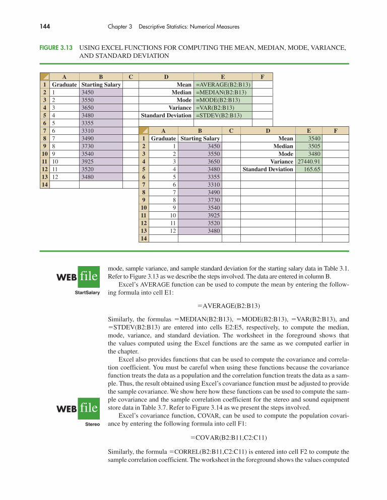
mode, sample variance, and sample standard deviation for the starting salary data in Table 3.1.Refer to Figure 3.13 as we describe the steps involved. The data are entered in column B.
Excel’s AVERAGE function can be used to compute the mean by entering the follow-ing formula into cell E1:
Similarly, the formulas �MEDIAN(B2:B13), �MODE(B2:B13), �VAR(B2:B13), and �STDEV(B2:B13) are entered into cells E2:E5, respectively, to compute the median, mode, variance, and standard deviation. The worksheet in the foreground shows that the values computed using the Excel functions are the same as we computed earlier in the chapter.
Excel also provides functions that can be used to compute the covariance and correla-tion coefficient. You must be careful when using these functions because the covariancefunction treats the data as a population and the correlation function treats the data as a sam-ple. Thus, the result obtained using Excel’s covariance function must be adjusted to providethe sample covariance. We show here how these functions can be used to compute the sam-ple covariance and the sample correlation coefficient for the stereo and sound equipmentstore data in Table 3.7. Refer to Figure 3.14 as we present the steps involved.
Excel’s covariance function, COVAR, can be used to compute the population covari-ance by entering the following formula into cell F1:
Similarly, the formula �CORREL(B2:B11,C2:C11) is entered into cell F2 to compute thesample correlation coefficient. The worksheet in the foreground shows the values computed
�COVAR(B2:B11,C2:C11)
�AVERAGE(B2:B13)
144 Chapter 3 Descriptive Statistics: Numerical Measures
FIGURE 3.13 USING EXCEL FUNCTIONS FOR COMPUTING THE MEAN, MEDIAN, MODE, VARIANCE,AND STANDARD DEVIATION
A B C D E F1 Graduate Starting Salary Mean =AVERAGE(B2:B13)2 1 3450 Median =MEDIAN(B2:B13)3 2 3550 Mode =MODE(B2:B13)4 3 3650 Variance =VAR(B2:B13)5 4 3480 Standard Deviation =STDEV(B2:B13)6 5 33557 6 33108 7 34909 8 373010 9 354011 10 392512 11 352013 12 348014
A B C D E F1 Graduate Starting Salary Mean 35402 1 3450 Median 35053 2 3550 Mode 34804 3 3650 Variance 27440.915 4 3480 Standard Deviation 165.656 5 33557 6 33108 7 34909 8 373010 9 354011 10 392512 11 352013 12 348014
fileWEBStereo
fileWEBStartSalary

Appendix 3.2 Descriptive Statistics Using Excel 145
using the Excel functions. Note that the value of the sample correlation coefficient (.93) isthe same as computed using equation (3.12). However, the result provided by the ExcelCOVAR function, 9.9, was obtained by treating the data as a population. Thus, we must ad-just the Excel result of 9.9 to obtain the sample covariance. The adjustment is rather sim-ple. First, note that the formula for the population covariance, equation (3.11), requiresdividing by the total number of observations in the data set. But the formula for the samplecovariance, equation (3.10), requires dividing by the total number of observations minus 1.So, to use the Excel result of 9.9 to compute the sample covariance, we simply multiply 9.9by n /(n � 1). Because n � 10, we obtain
Thus, the sample covariance for the stereo and sound equipment data is 11.
Using Excel’s Descriptive Statistics ToolAs we already demonstrated, Excel provides statistical functions to compute descriptivestatistics for a data set. These functions can be used to compute one statistic at a time (e.g., mean, variance, etc.). Excel also provides a variety of Data Analysis Tools. Oneof these tools, called Descriptive Statistics, allows the user to compute a variety of descriptive statistics at once. We show here how it can be used to compute descriptive sta-tistics for the starting salary data in Table 3.1.
Step 1. Click the Data tab on the RibbonStep 2. In the Analysis group, click Data AnalysisStep 3. When the Data Analysis dialog box appears:
Choose Descriptive StatisticsClick OK
sx y � �10
9 �9.9 � 11
FIGURE 3.14 USING EXCEL FUNCTIONS FOR COMPUTING COVARIANCE AND CORRELATION
A B C D E F G1 Week Commercials Sales Population Covariance =COVAR(B2:B11,C2:C11)2 1 2 50 Sample Correlation =CORREL(B2:B11,C2:C11)3 2 5 574 3 1 415 4 3 546 5 4 547 6 1 388 7 5 639 8 3 4810 9 4 5911 10 2 4612
A B C D E F G1 Week Commercials Sales Population Covariance 9.902 1 2 50 Sample Correlation 0.933 2 5 574 3 1 415 4 3 546 5 4 547 6 1 388 7 5 639 8 3 4810 9 4 5911 10 2 4612
fileWEBStartSalary

Step 4. When the Descriptive Statistics dialog box appears:Enter B1:B13 in the Input Range boxSelect Grouped By ColumnsSelect Labels in First RowSelect Output RangeEnter D1 in the Output Range box (to identify the upper left-hand corner
of the section of the worksheet where the descriptive statistics will appear)Select Summary statisticsClick OK
Cells D1:E15 of Figure 3.15 show the descriptive statistics provided by Excel. The boldface en-tries are the descriptive statistics we covered in this chapter. The descriptive statistics that arenot boldface are either covered subsequently in the text or discussed in more advanced texts.
Appendix 3.3 Descriptive Statistics Using StatToolsIn this appendix, we describe how StatTools can be used to compute a variety of descriptivestatistics and also display box plots. We then show how StatTools can be used to obtain covariance and correlation measures for two variables.
Descriptive StatisticsWe use the starting salary data in Table 3.1 to illustrate. Begin by using the Data Set Man-ager to create a StatTools data set for these data using the procedure described in the ap-pendix in Chapter 1. The following steps will generate a variety of descriptive statistics.
Step 1. Click the StatTools tab on the RibbonStep 2. In the Analyses Group, click Summary StatisticsStep 3. Choose the One-Variable Summary option
146 Chapter 3 Descriptive Statistics: Numerical Measures
FIGURE 3.15 EXCEL’S DESCRIPTIVE STATISTICS TOOL OUTPUT
A B C D E F1 Graduate Starting Salary Starting Salary2 1 34503 2 3550 Mean 35404 3 3650 Standard Error 47.825 4 3480 Median 35056 5 3355 Mode 34807 6 3310 Standard Deviation 165.658 7 3490 Sample Variance 27440.919 8 3730 Kurtosis 1.718910 9 3540 Skewness 1.091111 10 3925 Range 61512 11 3520 Minimum 331013 12 3480 Maximum 392514 Sum 4248015 Count 1216
fileWEBStartSalary

Step 4. When the One-Variable Summary Statistics dialog box appears:In the Variables section, select Starting SalaryClick OK
A variety of descriptive statistics will appear.
Box PlotsWe use the starting salary data in Table 3.1 to illustrate. Begin by using the Data SetManager to create a StatTools data set for these data using the procedure described in theappendix in Chapter 1. The following steps will create a box plot for these data.
Step 1. Click the StatTools tab on the RibbonStep 2. In the Analyses Group, click Summary GraphsStep 3. Choose the Box-Whisker Plot optionStep 4. When the StatTools—Box-Whisker Plot dialog box appears:
In the Variables section, select Starting SalaryClick OK
The symbol is used to identify an outlier and x is used to identify the mean.
Covariance and CorrelationWe use the stereo and sound equipment data in Table 3.7 to demonstrate the computationof the sample covariance and the sample correlation coefficient. Begin by using the DataSet Manager to create a StatTools data set for these data using the procedure described inthe appendix in Chapter 1. The following steps will provide the sample covariance and sam-ple correlation coefficient.
Step 1. Click the StatTools tab on the RibbonStep 2. In the Analyses Group, click Summary StatisticsStep 3. Choose the Correlation and Covariance optionStep 4. When the StatTools—Correlation and Covariance dialog box appears:
In the Variables sectionSelect No. of CommercialsSelect Sales Volume
In the Tables to Create section,Select Table of CorrelationsSelect Table of Covariances
In the Table Structure section select SymmetricClick OK
A table showing the correlation coefficient and the covariance will appear.
Appendix 3.3 Descriptive Statistics Using StatTools 147
fileWEBStartSalary
fileWEBStereo