Stats U2 Notes.notebook February 04, 2015

Jan 28­10:48 AM

Unit 2: Numerical Descriptive Measures

• Summation Notation• Measures of Central Tendency• Measures of Dispersion• Chebyshev's Rule• Empirical Rule• Measures of Relative Standing• Box Plots• z­scores

Jan 28­10:59 AM

Def 1: Numerical Descriptive Measures ­ describe numerical data in terms of summary properties

We will study 1. Measures of Central Tendency2. Measures of dispersion3. Measures of relative position

Before we get started we need to remember Summation Notation

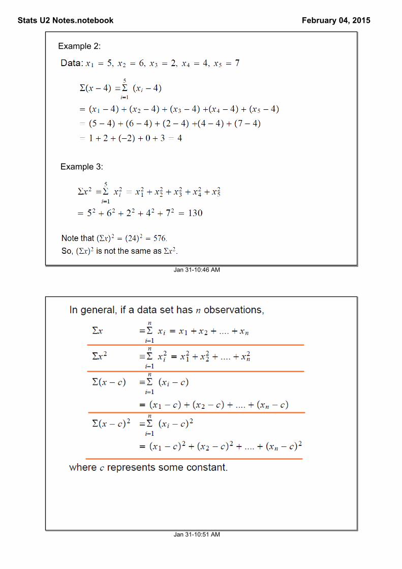
Example 1: Suppose a data set has n = 5 observations: 5, 6, 2, 4,7

find

So what would I do if I wanted

Stats U2 Notes.notebook February 04, 2015

Jan 31­10:46 AM

Example 2:

Example 3:

Jan 31­10:51 AM

Stats U2 Notes.notebook February 04, 2015

Jan 31­10:52 AM

1. Measures of Central Tendency

Def 2: Measures of Central Tendency ­ describe the center or typical value of the data. Typical observations in data sets include Mode, Mean, and Median

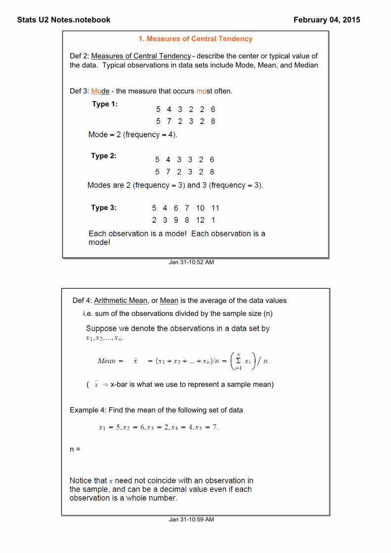
Def 3: Mode ­ the measure that occurs most often.

Type 1:

Type 2:

Type 3:

Jan 31­10:59 AM

Def 4: Arithmetic Mean, or Mean is the average of the data values

i.e. sum of the observations divided by the sample size (n)

( ⇒ x­bar is what we use to represent a sample mean)

Example 4: Find the mean of the following set of data

n =

Stats U2 Notes.notebook February 04, 2015

Jan 31­11:20 AM

Example 5: Let's take the same data set and change one of the data points to an outlier.

Jan 31­11:23 AM

Def 5: resistant measure a summary measure that is not affected by extreme observations.

Def 6: median (m) ­ the middle observation of a data set, after arranging the data in ascending order.

Example 6: Find the median of the data set: 5, 6, 2, 4, 7

1. Arrange observations in ascending order

2, 4, 5, 6, 7

2. Find the number of observations

­ if n is odd, the median is the middle observation

­ if n is even, the median is the average of the two middle observations

n = 5 (odd)

median = 5

3. the location of the median is found using

Stats U2 Notes.notebook February 04, 2015

Jan 31­12:41 PM

Example 7:

Find and compare the Mean, Median and Mode of the following.

55, 88, 99, 87, 110, 210, 65, 100, 75, 55

1. arrange in ascending order

55, 55, 65, 75, 87, 88, 99, 100, 110, 210

2. n = 10 (even)

Mean = 94.4

Median = 87.5

Mode = 55

Note: mode<median<mean

Jan 31­12:45 PM

Types of Distributions

1. Symmetric 2. Skewed Right 3. Skewed Left

Mean < Median<Mode

Helpful pneumonic:

Mean comes before median in the dictionary and will dictate skewness.

• if median<mean, skewed to the right

• if mean<median, skewed to the left.

The median is less sensitive to extreme observations; it is therefore a more resistant measure than the mean.

Stats U2 Notes.notebook February 04, 2015

Jan 31­1:00 PM

(mu)

(eta)

Jan 31­12:53 PM

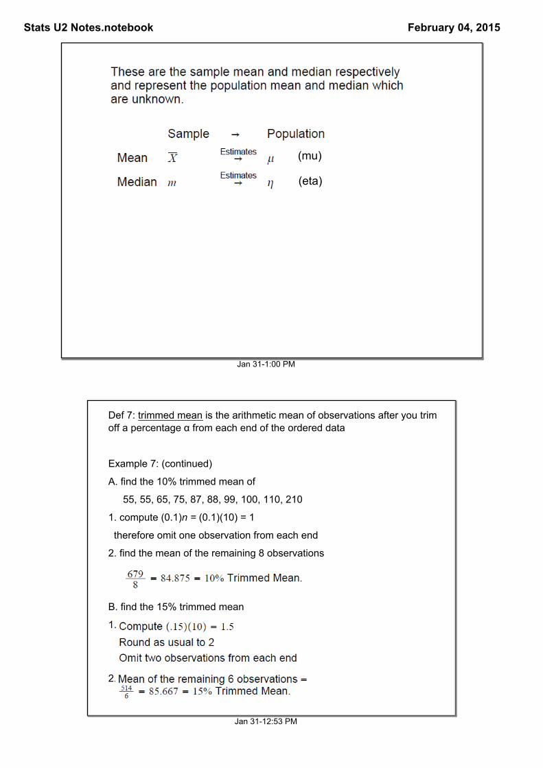
Def 7: trimmed mean is the arithmetic mean of observations after you trim off a percentage α from each end of the ordered data

Example 7: (continued)

A. find the 10% trimmed mean of

55, 55, 65, 75, 87, 88, 99, 100, 110, 210

1. compute (0.1)n = (0.1)(10) = 1

therefore omit one observation from each end

2. find the mean of the remaining 8 observations

B. find the 15% trimmed mean

1.

2.

Stats U2 Notes.notebook February 04, 2015

Jan 31­1:06 PM

2. Measures of Dispersion

Mean = Median = 45

These three data sets have the same center, but different spreads.

*write down data we will use it for multiple definitions

Def 8: measures of dispersion ­ measure to what extent data values are spread out about the center. Typical observations in the data set include range, variance, standard deviation and inter quartile range.

Example 8: Compare the mean and median of the following sets of data.

Jan 31­1:14 PM

Def 9: range the difference between the largest and smallest observations

Example 8 (continued): Find the range for data sets 1, 2, and 3

The range is the same for sets 1 and 2. Remember the center is 45 for each data set ­ note that the range is clearly no resistant

Stats U2 Notes.notebook February 04, 2015

Jan 31­1:23 PM

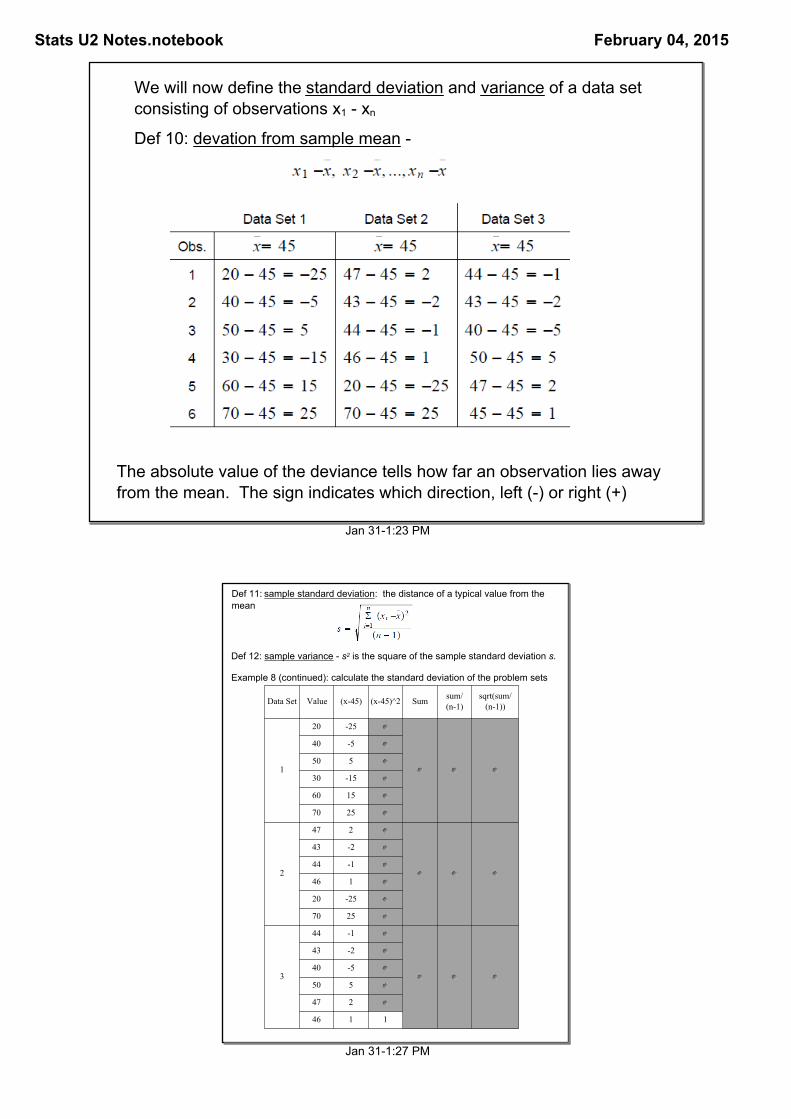
We will now define the standard deviation and variance of a data set consisting of observations x1 ­ xn

Def 10: devation from sample mean ­

The absolute value of the deviance tells how far an observation lies away from the mean. The sign indicates which direction, left (­) or right (+)

Jan 31­1:27 PM

Def 11: sample standard deviation: the distance of a typical value from the mean

Data Set Value (x­45) (x­45)^2 Sum sum/(n­1)

sqrt(sum/(n­1))

1

20 ­25

40 ­5

50 5

30 ­15

60 15

70 25

2

47 2

43 ­2

44 ­1

46 1

20 ­25

70 25

3

44 ­1

43 ­2

40 ­5

50 5

47 2

46 1 1

Def 12: sample variance ­ s2 is the square of the sample standard deviation s.

Example 8 (continued): calculate the standard deviation of the problem sets

Stats U2 Notes.notebook February 04, 2015

Jan 31­1:59 PM

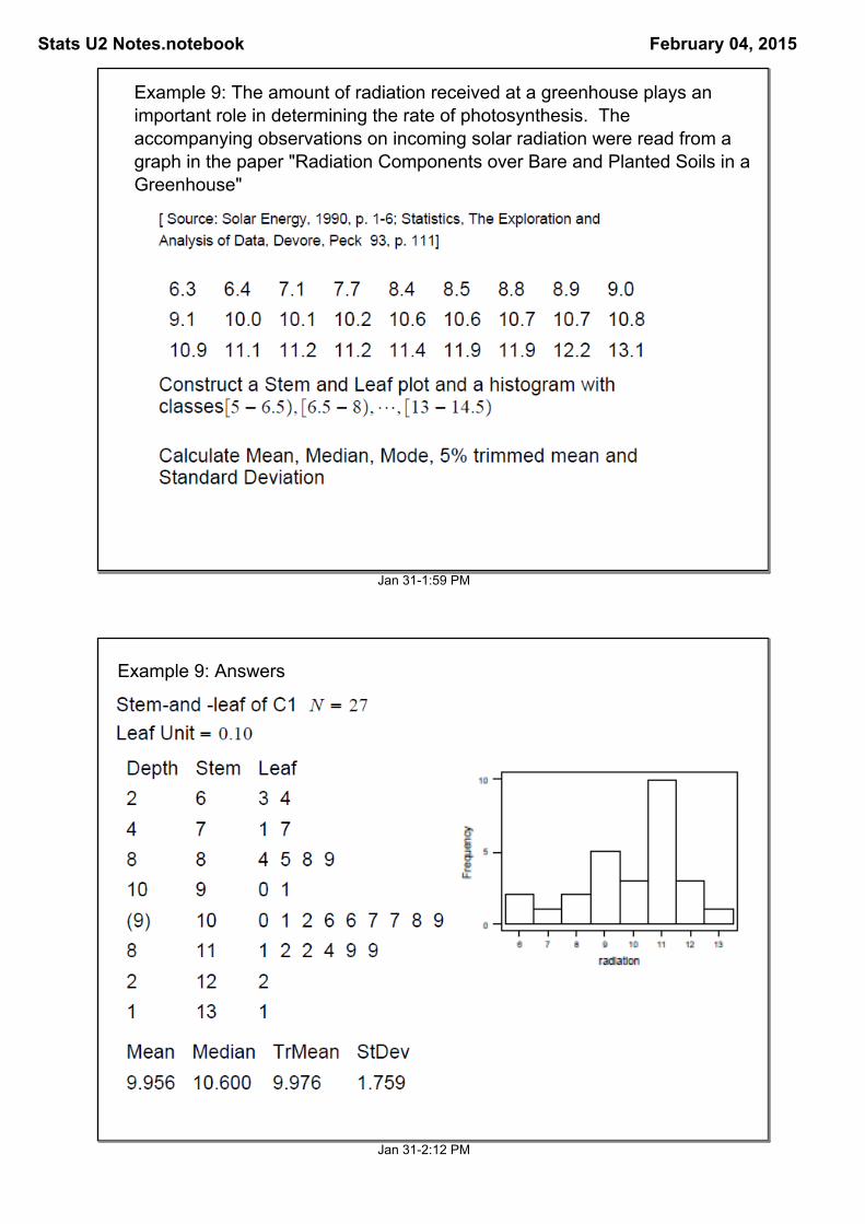
Example 9: The amount of radiation received at a greenhouse plays an important role in determining the rate of photosynthesis. The accompanying observations on incoming solar radiation were read from a graph in the paper "Radiation Components over Bare and Planted Soils in a Greenhouse"

Jan 31­2:12 PM

Example 9: Answers

Stats U2 Notes.notebook February 04, 2015

Jan 31­3:35 PM

Chebychev's Rule and Emperical Rule

As Statisticians we combine measures of central tendency with measures of variability to summarize a distribution for population or sample data sets.

Using these rules, it is possible to interpret the standard deviation and decide what proportions of observations generally are within

• 1 standard deviation of the mean

• 2 standard deviations of the mean

Jan 31­3:42 PM

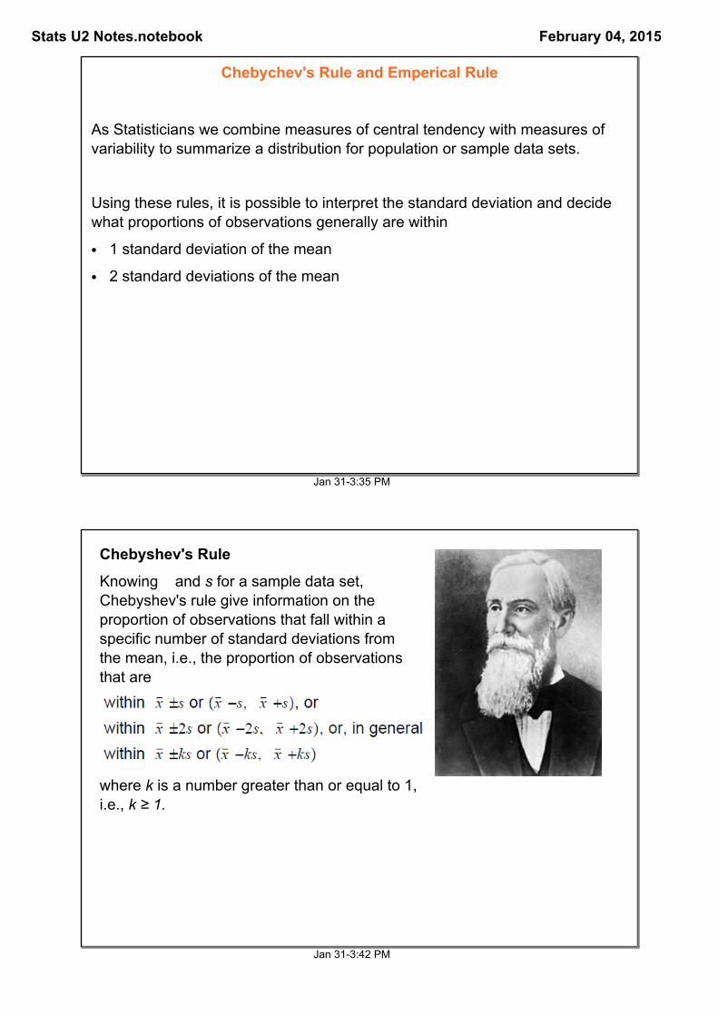
Chebyshev's Rule

Knowing and s for a sample data set, Chebyshev's rule give information on the proportion of observations that fall within a specific number of standard deviations from the mean, i.e., the proportion of observations that are

where k is a number greater than or equal to 1, i.e., k ≥ 1.

Stats U2 Notes.notebook February 04, 2015

Jan 31­3:54 PM

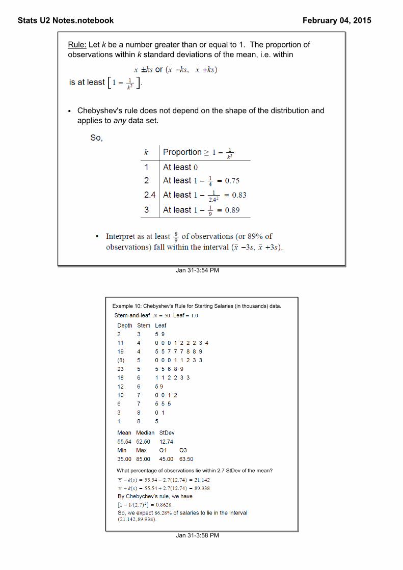
Rule: Let k be a number greater than or equal to 1. The proportion of observations within k standard deviations of the mean, i.e. within

• Chebyshev's rule does not depend on the shape of the distribution and applies to any data set.

Jan 31­3:58 PM

Example 10: Chebyshev's Rule for Starting Salaries (in thousands) data.

What percentage of observations lie within 2.7 StDev of the mean?

Stats U2 Notes.notebook February 04, 2015

Feb 1­12:53 PM

11

Jan 31­4:06 PM

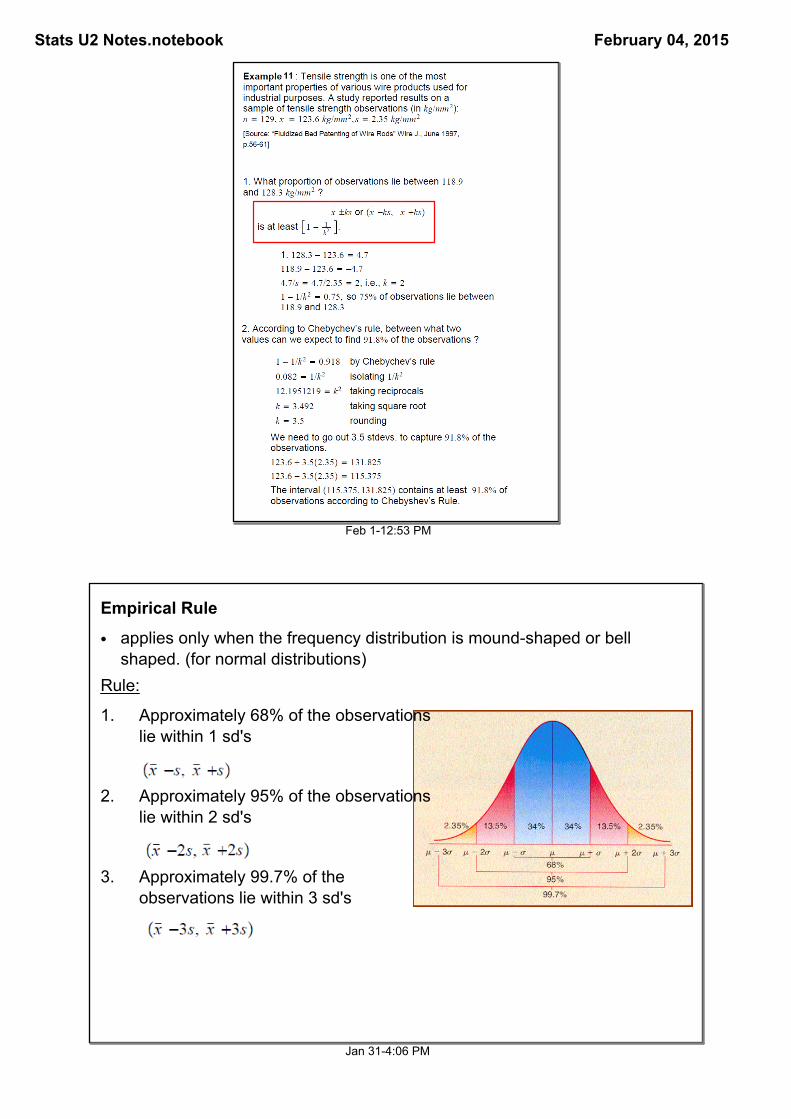
Empirical Rule

• applies only when the frequency distribution is mound­shaped or bell shaped. (for normal distributions)

Rule:

1. Approximately 68% of the observations lie within 1 sd's

2. Approximately 95% of the observations lie within 2 sd's

3. Approximately 99.7% of the observations lie within 3 sd's

Stats U2 Notes.notebook February 04, 2015

Jan 31­4:14 PM

12

Feb 1­1:02 PM

13

Stats U2 Notes.notebook February 04, 2015

Jan 31­4:19 PM

3. Measures of Relative Position

Def 13: Measure of relative position/standing ­ describe how a data value relates to other data values in a given data set. Typical observations in the data set include percentiles and quartiles

Def 14: pth percentile ­ a value such that p percent of the observations in the data set fall at or below that value.

ex ­ 95% of all test scores are at or below 650, whereas only 5% are above 650, then 650 is called the 95th percentile of the data set.

Procedure to find the pth percentile

Feb 1­12:33 PM

Example 10 (continued): Starting Salaries (in thousands) data.

Stats U2 Notes.notebook February 04, 2015

Feb 1­12:40 PM

Quartiles

Def 15: first (lower) quartile [Q1 or QL or P25]­ 25th percentile

i.e. 25% of the data is below it

Def 16: middle quartile [m] ­ 50th percentile or median

i.e. 50% of the data is below it

Def 17: upper quartile [Q3 or QU or P75] ­75th percentile

i.e. 75% of the data is below it

You can also obtain the quartiles by dividing the n ordered observations into a lower half and an upper half and find the median of each half

*if n is odd, the median is excluded from both halved when computing quartiles

Feb 1­1:07 PM

Box Plots

When to use: To highlight the center, spread, or any outliers in the data

How to Construct:

1. Draw a measurement scale

2. Construct a box with the ends

(hinges) at QL and QU. Show the

median (Q2) in the box.

3. From each hinge, calculate distance of 1.5 (IQR)

4. Whiskers are drawn from each hinge to most extreme

observations inside the inner fence.

5. From each hinge, calculate distances 3.0(IQR)

6. If an observation in the data set falls between the inner and outer fences, it is a mile outlier

7. Those falling outside the outer fence, are extreme outlier

Def 18: interquartile range ­ QU ­ QL, it is a measure of variability that is not sensitive to the presence of outliers unlike the standard deviation.

Def 19:

Stats U2 Notes.notebook February 04, 2015

Feb 1­1:39 PM

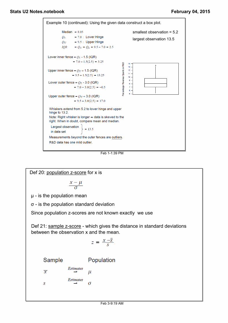
Example 10 (continued): Using the given data construct a box plot.

smallest observation = 5.2

largest observation 13.5

Feb 3­9:19 AM

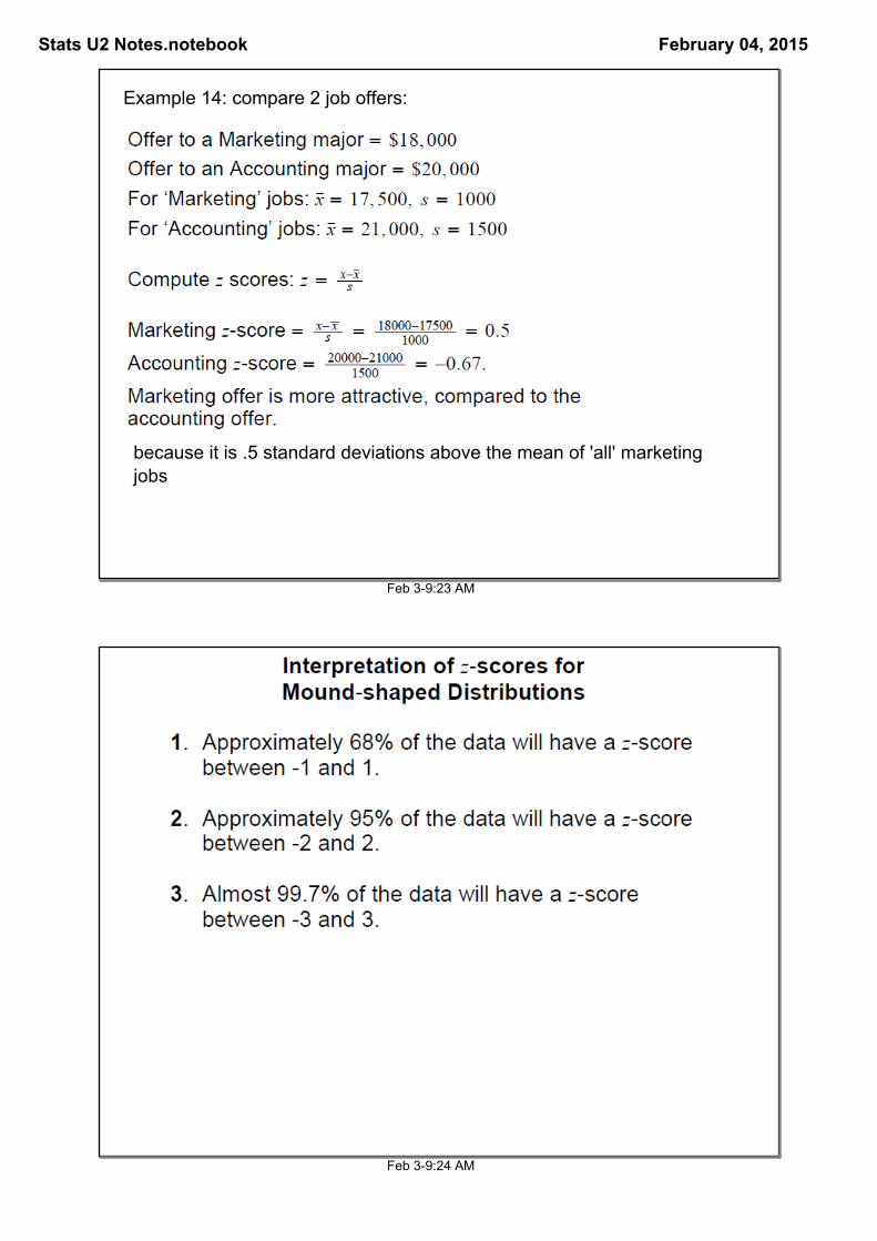
Def 20: population z­score for x is

μ ­ is the population mean

σ ­ is the population standard deviation

Since population z­scores are not known exactly we use

Def 21: sample z­score ­ which gives the distance in standard deviations between the observation x and the mean.

Stats U2 Notes.notebook February 04, 2015

Feb 3­9:23 AM

Example 14: compare 2 job offers:

because it is .5 standard deviations above the mean of 'all' marketing jobs

Feb 3­9:24 AM

Stats U2 Notes.notebook February 04, 2015

Feb 3­9:25 AM

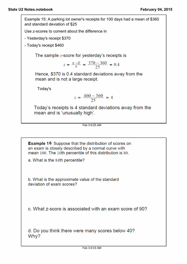
Example 15: A parking lot owner's receipts for 100 days had a mean of $360 and standard deviation of $25

Use z­scores to coment about the difference in

­ Yesterday's receipt $370

­ Today's receipt $460

Today's

Feb 3­9:33 AM

6