design and analysis of mechanically laminated timber … dissertation.pdf · design and analysis of...
TRANSCRIPT

Design and Analysis of
Mechanically Laminated Timber Beams
Using Shear Keys
By
Joseph F. Miller
A Dissertation
Submitted in partial fulfillment
of the requirements for the degree of
Doctor of Philosophy
in Civil Engineering
Michigan Technological University
2009
Copyright © Joseph F. Miller 2009

This dissertation, “Design and Analysis of Mechanically Laminated Timber Beams using
Shear Keys,” is hereby approved in partial fulfillment of the requirements for the degree
of Doctor of Philosophy in the field of Civil Engineering.
Department of Civil and Environmental Engineering
Signatures:
Dissertation Adviser __________________________________________
Dr. William Bulleit, PE
Department Chair __________________________________________
Dr. William Bulleit, PE
Date __________________________________________

iii
Acknowledgements
My appreciation goes to Trillium Dell Timberworks (Knoxville, IL) for supplying
the white oak key stock, and to Coldwater Veneer (Coldwater, MI) for supplying the
clear yellow poplar timbers for the physical testing component of the research. I’d also
like to thank Fastenmaser/OMG and Wurth Construction Specialty Supply for supplying
the screws.
I’d like to thank my advisers for their help and support; in particular Dr. Bulleit,
who, despite my jejune and somewhat contumelious attempts, ensured some pellucidity
in my writing. Dr. Brungraber was also a guiding force throughout this process,
providing invaluable and practical insights. I am moreover indebted to my wife for her
patient support throughout this endeavor. Prost.
iv
Abstract
Small timber layers can be mechanically laminated into a larger timber cross-
section using shear keys to prevent slip between the layers. These mechanically
laminated beams are commonly referred to as keyed beams, and their use has a strong
historical precedence. Current building codes and design standards do not provide
adequate guidelines for the analysis and design of keyed beams.
This project examined the applicability of an interlayer slip model to predict the
partially composite behavior of the keyed beams. Solutions to the interlayer slip model
for common loading configurations were developed, as were stiffness parameters for the
semi-rigid wooden shear keys used to provide composite action.
Small scale testing was conducted on the wooden shear key components to verify
the stiffness parameters. Full-scale testing of yellow poplar keyed beams using white oak
and Parallam PSL shear keys was also performed to verify the interlayer slip model’s
ability to predict the strength and stiffness of specific specimens. A comparison to
historical keyed beam test data was also conducted.
The interlayer stiffness model, as well as the analytical shear key stiffness
parameters, was able to accurately predict both the behavior for the full-scale keyed
beams tested specifically for this research as well as the historic keyed beam behavior.
Shear key configuration, moisture content, and clamping connector stiffness all played
significant roles in the actual keyed beam stiffness.

v
Table of Contents
1 Introduction............................................................................................................... 1 1.1 Background Information..................................................................................... 1
1.2 Research Objectives............................................................................................ 2
1.3 Literature Review................................................................................................ 3
1.3.1 Historical Literature ................................................................................... 3
1.3.2 Theoretical & Modern Literature ............................................................. 10
1.3.3 Design Literature ...................................................................................... 11
2 Theoretical Model ................................................................................................... 13 2.1 Partial Interlayer Slip Model Derivation........................................................... 14
2.1.1 Beam Solution for n-Layers ...................................................................... 15
2.1.2 Beam Solution for Two Layers.................................................................. 19
2.1.3 Beam Solution for Three Layers ............................................................... 20
2.2 Solutions for the Two Layer Model with Uniform Loading............................. 22
2.2.1 Axial Force in Each Layer........................................................................ 22
2.2.2 Bounds on Uniformly Distributed Load Solution ..................................... 23
2.3 Other Loading Conditions................................................................................. 25
2.3.1 Numerical Integration............................................................................... 25
2.3.2 Linear-Elasticity and Superpositioning .................................................... 25
2.4 Stress Distribution............................................................................................. 28
2.5 Shear Keys ........................................................................................................ 30
2.5.1 Shear Key Stiffness.................................................................................... 32
2.5.2 Shear Key Stiffness Coefficients................................................................ 36
2.6 Beam Efficiency................................................................................................ 39
3 Physical Testing Overview ..................................................................................... 42 3.1 Timber and Key Species ................................................................................... 42
3.1.1 Timber Species Selection .......................................................................... 42
3.1.2 Shear Key Species Selection ..................................................................... 43
3.2 Key Configuration ............................................................................................ 45
3.2.1 Key Orientation......................................................................................... 45
3.2.2 Grain Direction......................................................................................... 46
3.2.3 Key Size..................................................................................................... 49
3.2.4 Wedge Slope.............................................................................................. 50
3.3 Clamping Connectors........................................................................................ 51
3.3.1 Connector Type......................................................................................... 51
3.3.2 Connector Placement................................................................................ 53
3.3.3 Connector Quantity................................................................................... 53
3.4 Beam Size ......................................................................................................... 54
3.5 Loading Configuration...................................................................................... 55
3.6 Key Layout in Keyed Beam.............................................................................. 57
4 Small Scale Testing ................................................................................................. 60 4.1 Testing Apparatus ............................................................................................. 60
4.2 Modulus of Elasticity and Modulus of Rupture................................................ 61
4.2.1 Static Bending Test Procedure.................................................................. 61
vi
4.2.2 Static Bending Test Results....................................................................... 62
4.2.3 Adjustment of Modulus of Elasticity for Shear Deformation.................... 64
4.3 Screw Axial Stiffness and Withdrawal Capacity.............................................. 65
4.3.1 Screw Withdrawal Test Procedure ........................................................... 66
4.3.2 Screw Withdrawal Test Results................................................................. 67
4.4 Shear Key Stiffness........................................................................................... 70
4.4.1 White Oak Shear Key Test Results............................................................ 74
4.4.2 Parallam PSL Shear Key Test Results ...................................................... 77
4.4.3 Shear Key Test Comparison to Stiffness Model........................................ 81
4.5 Screw Shear (Lateral) Stiffness ........................................................................ 82
4.5.1 Screw Shear Test Procedure..................................................................... 83
4.5.2 Screw Shear Specimen Test Results.......................................................... 83
4.6 Moisture Content and Specific Gravity ............................................................ 86
4.6.1 Adjustments in Modulus of Elasticity Based on Moisture Content........... 86
4.6.2 Adjustments in Modulus of Elasticity Based on Specific Gravity ............. 87
5 Full Scale Beam Testing ......................................................................................... 90 5.1 Beam Fabrication .............................................................................................. 90
5.2 Testing Apparatus ............................................................................................. 92
5.3 Test Results....................................................................................................... 94
5.3.1 Full and Stacked Beams............................................................................ 94
5.3.2 Keyed Beams with White Oak Shear Keys ................................................ 97
5.3.3 Keyed Beams with Parallam PSL Shear Keys ........................................ 101
5.4 Adjustments to Test Results............................................................................ 103
5.4.1 Moisture Content and Specific Gravity................................................... 104
5.4.2 Variations in Cross Section .................................................................... 106
5.4.3 Test Frame Compliance.......................................................................... 106
6 Analysis of the Interlayer Slip Model using Full Scale Test Data .................... 108 6.1 Comparison of Test Data ................................................................................ 108
6.1.1 Interlayer Slip Model Input Parameters ................................................. 108
6.1.2 Analysis Results ...................................................................................... 112
6.2 Shear Key Spacing Methodology ................................................................... 114
6.2.1 Simplified Approach................................................................................ 115
6.2.2 Shear Stud / Composite Beam Approach ................................................ 115
6.2.3 Tributary Length Approach .................................................................... 117
6.2.4 Recommended Spacing Calculation ....................................................... 118
6.3 Material Parameter Sensitivity........................................................................ 119
6.3.1 Modulus of Elasticity of Timbers ............................................................ 120
6.3.2 Cross-grain Modulus of Elasticity .......................................................... 121
6.3.3 Clamping Connectors ............................................................................. 123
6.3.4 Key Size................................................................................................... 125
6.4 Comparison to Kidwell’s Test Data................................................................ 126
6.4.1 Determining Material Properties ........................................................... 127
6.4.2 Brunel’s Beam......................................................................................... 129
6.4.3 Joggled Beam.......................................................................................... 131
6.4.4 Three Layer Beam................................................................................... 135

vii
6.4.5 Discussion of Results .............................................................................. 138
7 Ultimate Stress ...................................................................................................... 139 7.1 Predication of Failure Load ............................................................................ 139
7.2 Comparison to Full Scale Testing................................................................... 140
7.3 Comparison to Kidwell’s Historical Testing .................................................. 142
7.4 Discussion of Results...................................................................................... 143
8 Design Procedure .................................................................................................. 145 8.1 Shear Key and Clamping Connector Design .................................................. 145
8.1.1 Shear Key and Timber Compressive Strength ........................................ 146
8.1.2 Shear Key Spacing .................................................................................. 147
8.1.3 Clamping Strength Requirements ........................................................... 150
8.2 Full Design Procedure..................................................................................... 151
8.2.1 Beam Bending Stress............................................................................... 151
8.2.2 Beam Stiffness ......................................................................................... 153
8.3 Simplified Design Procedure .......................................................................... 153
9 Conclusions............................................................................................................ 156 9.1 Summary......................................................................................................... 156
9.2 Qualified Recommendations........................................................................... 157
9.3 Future Research .............................................................................................. 160
10 References .......................................................................................................... 164
Appendix A – Solution for Two-Layer Beam with a Uniformly Distributed Load 169
Appendix B – Solution for Two-Layer Beam with Point Load at any Point........... 170
Appendix C – Solution for Two-Layer Beam with Symmetrically Placed Point
Loads .............................................................................................................................. 176
Appendix D – Calculations for Quantity of Clamping Connectors ......................... 182
Appendix E – Longitudinal Modulus of Elasticity and Shear Modulus in Bending
Tests................................................................................................................................ 184 E.1 Determination from Testing ................................................................................. 184
E.2 Comparison of Full Depth and Simple Stacked Beam Deflection ....................... 186
Appendix F – Adjustment of Shear Keys Test Stiffness............................................ 188
Appendix G – Calculation of Slip in a Simple Stacked Beam .................................. 189
Appendix H – Interlayer Slip Calculations for Full-Scale Test Data....................... 191 H.1 Analysis of Test Data from this Research............................................................ 191
H.2 Analysis of Test Data from Prior Research ......................................................... 195
Appendix I – Stress Calculations................................................................................. 200

viii
Table of Tables
Table 4-1 Static bending test results ................................................................................. 63
Table 4-2 Screw withdrawal test results ........................................................................... 68
Table 4-3 Results from white oak shear key tests............................................................. 75
Table 4-4 Results from Parallam PSL shear key tests ...................................................... 78
Table 4-5 Key stiffnesses from physical tests as well as the theoretical model ............... 81
Table 4-6 Results from screw shear tests.......................................................................... 84
Table 5-1 Full-scale beam test results............................................................................... 96
Table 5-2 Adjusted stiffness values for full-scale beam tests......................................... 105
Table 5-3 Differences in stiffness from test frame compliance...................................... 107
Table 6-1 Physical data on keyed beam tests for use with the interlayer slip model ..... 109
Table 6-2 Comparison of analytical and full-scale testing stiffnesses............................ 112
Table 6-3 Comparison of various methods for determining shear key spacing ............. 117
Table 6-4 Variations in stiffness with changes in timber modulus of elasticity............. 121
Table 6-5 Comparison of Brunel's beam stiffnesses to the interlayer slip model........... 130
Table 6-6 Comparison of joggled beam stiffnesses to interlayer slip model.................. 133
Table 6-7 Comparison of joggled beam stiffnesses to interlayer slip model.................. 135
Table 6-8 Comparison of three-layer beam stiffness to interlayer slip model................ 137
Table 7-1 Stress at maximum load for full-scale beam tests .......................................... 140
Table 7-2 Stress at maximum load for Kidwell’s beam tests ......................................... 143

ix
List of Figures
Figure 1-1 Two-layer keyed beam using wood shear keys to generate composite action.. 2
Figure 1-2 "Why wood bends, breaks, and stays stiff, and how to make it stiff." (Leupold,
1726). .......................................................................................................................... 4
Figure 1-3 - Tredgold's beams: (a) Keyed beam, (b) Joggled beam with cast iron wedge
(Tredgold, 1820) ......................................................................................................... 6
Figure 1-4 - Mahan's and Rankine's proposed beams, respectively (Mahan, 1886;
Rankine, 1889)............................................................................................................ 7
Figure 1-5 - Derevyagin's beam which includes prestressing before installation of the
shear keys (Karlsen, 1967).......................................................................................... 9
Figure 2-1 Solid beam unloaded and subjected to positive bending moment .................. 13
Figure 2-2 Simple stacked beam unloaded and subjected to positive bending moment .. 14
Figure 2-3 Section through an n-layer beam..................................................................... 16
Figure 2-4 Stress diagram for an n-layer beam................................................................. 16
Figure 2-5 Superpositioning of pointloads ....................................................................... 27
Figure 2-6 Normal stress diagrams for an arbitrary full depth (dashed line) and built up
(solid line) beam ....................................................................................................... 30
Figure 2-7 Side view of (a) square and (b) inclined shear keys along with (c) a top view
showing the wedge shape of the shear keys.............................................................. 32
Figure 2-8 Inclined shear key ........................................................................................... 33
Figure 2-9 Deformed inclined key.................................................................................... 33
Figure 2-10 Springs-in-series model of the shear key ...................................................... 34
Figure 2-11 Displacement components of a shear key ..................................................... 35
Figure 2-12 Shear flow in partially composite beams subjected to (a) two concentrated
loads and (b) a uniformly distributed load. ............................................................... 40
Figure 3-1 2.5 inch thick shear key wedge dimensions .................................................... 48
Figure 3-2 Solid sawn parallel-to-the-grain wedges are prone to splitting during
installation................................................................................................................. 48
Figure 3-3 (a) Long and (b) short shear key configurations ............................................. 50
Figure 3-4 Forces acting on a pair of wedges ................................................................... 51
Figure 3-5 Double threaded log screw.............................................................................. 53
Figure 3-6 Key placement and screw location on keyed beams used in the full-scale
testing........................................................................................................................ 53
Figure 3-7 Loading configuration for full scale beam testing .......................................... 56
Figure 3-8 Assumed shear stress distribution at shear key notch ..................................... 58
Figure 4-1 Setup for static bending tests........................................................................... 62
Figure 4-2 Static bending test compression failure followed by a simple-tension failure 63
Figure 4-3 Load-displacement plots for static bending tests ............................................ 64
Figure 4-4 Screw push-through (e.g. withdrawal) testing ................................................ 67
Figure 4-5 Load-displacement plots for screw withdrawal tests ...................................... 69
Figure 4-6 Screw withdrawal testing showing (a) entry of screw, (b) exit of screw, and (c)
section through screw hole after screw had been removed....................................... 70
Figure 4-7 8in long shear key test configuration .............................................................. 73
Figure 4-8 5in long shear key test configuration .............................................................. 74

x
Figure 4-9 Load-slip plots for white oak shear key tests .................................................. 75
Figure 4-10 Load-spread plots of white oak shear key tests............................................. 77
Figure 4-11 Load-slip plots for Parallam PSL shear key tests.......................................... 78
Figure 4-12 (a) 8 inch white oak key compressed uniformly, (b) 5 inch white oak key
with uneven compression due to rolling, (c) compression of the timber end-grain
when using Parallam PSL keys, (d) uniform spreading of side member and (e)
uneven spreading with rolling of side member for Parallam PSL key tests. ............ 80
Figure 4-13 Load-slip plots for screw shear specimen tests ............................................. 84
Figure 4-14 Yielding of screw subjected to shear (lateral) loading.................................. 85
Figure 4-15 Localized crushing of wood fibers from screw subjected to shear (lateral)
loading....................................................................................................................... 85
Figure 4-16 Comparison of Wood Handbook MOE equations to test data (typical) ....... 88
Figure 5-1 (a) Paired and notched timbers with checks on the horizontal faces and (b)
clamping apparatus used when installing the screws................................................ 92
Figure 5-2 Full scale beam test configuration................................................................... 93
Figure 5-3 Ring-shake and checking in the full depth beam ............................................ 95
Figure 5-4 Load-deflection plots of full-scale beam tests ................................................ 96
Figure 5-5 Keyed beam using white oak shear keys under load....................................... 98
Figure 5-6 Load-slip plots for white oak shear key tests .................................................. 99
Figure 5-7 Cracked keyed beam using white oak shear keys ......................................... 100
Figure 5-8 Crack propagating from re-entrant notch corner........................................... 100
Figure 5-9 Parallam PSL-keyed beam under load .......................................................... 103
Figure 6-1 Comparison of load-deflection plots and interlayer slip model solutions..... 113
Figure 6-2 Assumed shear key spacing using a composite beam approach ................... 116
Figure 6-3 Assumed shear key spacing using tributary length approach ....................... 118
Figure 6-4 Relationship between elastic ratio and calculated beam stiffness for each beam
test ........................................................................................................................... 122
Figure 6-5 Difference between test and model stiffness with varying elastic ratios ...... 123
Figure 6-6 Relationship between the number of clamping screws and modeled beam
stiffness ................................................................................................................... 124
Figure 6-7 Relationship between key length and model stiffness .................................. 125
Figure 6-8 Key configuration in Brunel's beams (Kidwell, 1898) ................................. 129
Figure 6-9 Load-deflection plots for Brunel's beams (Kidwell, 1898)........................... 130
Figure 6-10 Key configuration for joggled beam using white oak keys (Kidwell, 1898)
................................................................................................................................. 131
Figure 6-11 Key configuration for joggled beam using cast iron keys (Kidwell, 1898) 132
Figure 6-12 Load-deflection plots for joggled beams using white oak keys .................. 133
Figure 6-13 Load-deflection plots for joggled beams using cast iron keys .................... 134
Figure 6-14 Key configuration for three-layer beam using white oak keys (Kidwell, 1898)
................................................................................................................................. 136
Figure 6-15 Load-deflection plots for three-layer beam using white oak keys .............. 137
Figure 8-1 Shear key spacing for a beam with (a) two concentrated point loads, and (b) a
uniformly distributed load....................................................................................... 149
Figure 8-2 Clamping connector geometry ...................................................................... 151

1
1 Introduction
1.1 Background Information
There is a long standing historical precedent to build structures from large
timbers. The use of timbers is due in part to wood’s structural characteristics,
workability, natural aesthetical appeal, as well as being a renewable resource. With the
advent of balloon framing, reinforced concrete, and structural steel, along with new
structural requirements, there was a logical progression away from building with heavy
timber (Goldstein, 1999). However, none of the reasons that originally made building
with timber popular have diminished. As the emphasis increases for use of renewable
resources and materials with a natural aesthetic, timber again is increasing in popularity
(Benson, 1999).
With this rebound in popularity, adapting the historical methods of using timber
to meet more modern building requirements is essential to ensure its long term viability.
Unlike more traditional buildings, modern timber structures are expected meet stringent
building codes, which can result in longer spans, tighter deflection controls, and heavier
loads. Likewise, excessive pressure on a renewable resource can hinder the industry, thus
better stewardship of the materials at hand is key.
For long or heavily loaded spans using solid sawn timber, high grade and large
cross sections are required to adequately carry the load. Due to a limited number of large
trees for harvesting, the price, and availability, if available at all, of the required timber
size can be quite prohibitive. The use of glue-laminated timbers (glulams), where small
dimensional lumber is glued together to create a high grade composite cross section,

2
addresses these availability concerns. However, glulams do not have strong aesthetic
appeal to most heavy timber enthusiasts, and others have concerns about the adhesives
used in fabrication.
An alternative to the large solid sawn timber cross sections and glulams is to use
mechanically laminated timbers. A common example, and one that is the focus of this
research, is often referred to as a “keyed beam” because of the shear keys between layers.
Timbers of smaller cross section (which come from smaller, more readily available trees)
are used to generate a composite cross section. The interaction between timbers is
generated using a series of shear keys. One method is to use wooden wedges for the
shear keys, which are typically left exposed on the sides and help provide a visual appeal
that many find attractive. Figure 1-1 shows a keyed beam with a common configuration
of wooden shear keys. Currently there are no design procedures to directly address the
analysis and design of these beams.
Figure 1-1 Two-layer keyed beam using wood shear keys to generate composite action
1.2 Research Objectives
The goal of this study is to develop an accurate behavioral model for mechanically
laminated timber beams that provide partial interaction through the use of wood shear
keys. The behavioral model will be compared against physical testing to verify its
performance.

3
The objectives of this research are broken into four separate stages. These stages
include:
1. Developing a n-ply solution to the classical interlayer slip model, coupled
with specific solutions for common loading configurations for the two-
layer solution.
2. Formulating stiffness models for inclusion into the interlayer slip model
that accurately represent common wooden shear key configurations.
3. Determining experimentally the strength and stiffness of full sized keyed
beams as well as individual key and screw components.
4. Developing a procedure than can be readily implemented by practicing
engineers for the design and analysis of keyed beams.
1.3 Literature Review
The concept of mechanically joining timbers for the purpose of generating a larger
composite bending section is not new. Limited availability of large timber in Europe
before the invention of reliable adhesives necessitated their use.
1.3.1 Historical Literature
The earliest documentation that was found during this research, suggesting the use
of shear keys to increase the depth of beams, was an article by Jacob Leupold, published
in Leipzig, Germany (Leupold, 1726). The author’s main focus was on bridge
construction and he suggested the use of keyed beams as bridge girders as shown in
Figure 1-2.

4
Figure 1-2 "Why wood bends, breaks, and stays stiff, and how to make it stiff." (Leupold, 1726).

5
The first notable technical documentation, at least in English, was published in
England in 1820 by Thomas Tredgold, an outspoken civil engineer (Tredgold, 1820). He
suggested the use of solid shear keys to limit interlayer slip. He also recommended
tapering the upper beam, such that the ends of the beams where slightly shallower than
the middle, so solid metal bands could be driven onto the ends to provide the clamping
force, much in the same way metal bands are driven onto wooden barrels. Tredgold also
indicated a strong preference for a joggled beam (mated saw tooth type indentations
between layers) using a cast iron wedge to ensure tight bearing faces. These beams are
shown in Figure 1-3. Of note are the incredible difficulties in fabricating Tredgold’s
beams. Procuring exact dimension metal straps to ensure proper clamping was also
problematic. Also, the taper makes supporting a floor or flat roof difficult. Likewise, the
fabrication tolerances required to make an appropriate joggled beam are extremely labor
intensive, and the net depth of the members is reduced. Use of the cast iron wedge to
ensure tight fitting faces was novel, but this will induce tensile stresses in the bottom
member, which also has a hole drilled through it at the point of maximum stress. Once
bending stress is applied, it will further increase the tensile stress in the bottom member,
ensuring that the allowable capacity of this beam will be considerably lower than a fully
composite beam.

6
(a)
(b)
Figure 1-3 - Tredgold's beams: (a) Keyed beam, (b) Joggled beam with cast iron wedge (Tredgold,
1820)
Many other publications during the 19th
century included similar descriptions or
verbatim copies of built-up beams as those proposed by Tredgold (e.g., Trautwine, 1862).
Other authors, such as Mahan (1886) and Rankine (1889), offered additional theoretical
improvements to Tredgold’s previously proposed beam. Mahan’s addition was to use
multiple layers of beams joggled together. He stated that to his knowledge no one had
ever tried such a beam, and due to constructability concerns, no effort has probably ever
been made since. Rankine suggested using through bolts, either square through the
timbers, or preferably at an incline to provide the clamping force, rather than fitted metal
bands. Mahan and Rankine’s suggestions are shown in Figure 1-4.

7
Figure 1-4 - Mahan's and Rankine's proposed beams, respectively (Mahan, 1886; Rankine, 1889)
During the mid 19th
century, with the industrialization of the world, and in
particular the development of vast systems of railroads, great demands were placed on
regional and national timber supplies. These demands were caused not only by the
inherent need for timber in the railroad industry for things such as railroad ties and bridge
girders, but also for the development of industrial buildings and residential structures.
Many railroads developed their own method for joining beams into deeper cross sections,
typically with the use of cast iron and steel sections, for use as bridge girders. Of
particular merit is an article by Snow (1895), of the Boston and Main Railroad, on the use
of steel keys for built-up girders. His discussion includes guidance on required clamping
forces as well as suggestions for spacing according to the “intensity of shearing strain.”
He also advocates using the full depth of the combined beam for determining stresses
(full composite action).
Railroad bridge construction was not limited to the United States, however. Many
railroad bridges were built throughout continental Europe, in particular Germany and
Austria, that used zusammengesetzte Balkenträger (composite girders) along with
verdübelten Trägern (keyed beams). A text by a Finnish professor, Michael Strukel,

8
documents many types of railroad bridges, some of which used keyed beams (Strukel,
1900).
Academic research was conducted by Prof. Dr. Forchheimer in Aachen, Germany
on the use of keyed and built-up beams (Forchheimer, 1892). He investigated several
types of keyed and built-up beams, and provided some guidance on the proper size and
orientation of the keys. Forchheimer observed that the rotation of the keys, either caused
by improper key sizing or insufficient clamping action, greatly reduced the capacity of
the beam. He also noted that the grain orientation of the keys plays a significant role in
the efficiency of the beam.
But, perhaps Edgar Kidwell, a professor at the Michigan College of Mines, has
the most complete and academically rigorous review of keyed beams (Kidwell, 1898).
The declining availability of locally available timber coupled with an increasing demand
for timber use in mining was the catalyst for Kidwell’s testing of full sized specimens
with various wooden key configurations, as well as beams using iron and steel keys.
Kidwell (1898) concluded that indeed most of the published contemporary
information available on keyed beams was of little practical merit. He also concluded:
(1) cast iron keys will result in greater stiffness than wooden keys; (2) loosening of
clamping bolts from timber shrinkage has a substantial impact on stiffness; (3) inclined
keys are less desirable than square keys; and (4) keyed beams can achieve approximately
90% of the capacity of the a full depth, solid beam.
Shortly after Kidwell’s research, steel and concrete became popular as structural
materials, and little else was published on the topic for 70 years. What little was
published included little new information (Warren, 1910). Others just repeated the

9
conclusions of those before them in a concise and easy to follow format, but without
offering any new insights (Durm and Esselborn, 1908; Jacoby, 1909).
In 1967, Karlsen published an inclusive text on timber engineering, translated
from Russian, that included several sections on keyed beams. Karlsen provides design
recommendations for shear key sizes, correction factors for the beam stiffness, and a
strong preference for inclined keys. Karlsen also makes a reference to Derevyagin’s
beams, which are keyed beams precambered and connected with wooden plates, rather
than shear keys. The fabrication of this beam can be seen in Figure 1-5. Unfortunately
no additional information about the Derevyagin’s beam was provided for further
investigation.
Figure 1-5 - Derevyagin's beam which includes prestressing before installation of the shear keys
(Karlsen, 1967).

10
1.3.2 Theoretical & Modern Literature
From a theoretical standpoint, Newmark, Seiss, and Viest (1951), commonly
referred to as Newmark’s approach, developed a relationship for stacked beams that have
partial interaction between the layers. While their development was intended for
steel/concrete T-beams, it applies in general to any geometric and material
configurations. The linear-elastic theory allows for some slip between the two layers by
solving a series of differential equations relating the rate of change of slip and strains in
the two layers. Since the rate of slip and strains are load dependent, solving the system of
equations requires a separate solution for each loading condition. Coincidentally, at the
same time as their development (Newmark et al., 1951), others in Russia (Pleshkov,
1952) and Sweden (Granholm, 1949) independently developed similar approaches. Only
abstracts of these two sources could be found translated into English, so the full body of
their work has not been reviewed.
Goodman (1967) expanded on Newmark’s development for nail laminated
dimensional lumber with two and three plies. A comparison between the approaches of
Newmark (1951), Pleshkov (1952), and Granholm (1949) was also made. Goodman
went on to expand his research and co-authored additional papers verifying his
mathematical model (e.g. Goodman & Popov, 1968).
Additional authors have expanded on Newmark and Goodman for various specific
problems. Wheat and Calixto (1994) investigated the effect of non-linear connectors at
the interface using energy methods. Shear deformation was addressed by Schnabl et al.
(2007), who showed that it has substantial influence on the vertical deflection of
partially-composite beams. Not surprisingly, shear deformation had a higher contribution

11
to the overall deflection as composite action approached that of a full depth beam, as well
as with beams having small span to depth ratios.
In order to facilitate computer modeling of beams with interlayer slip, research
has also been conducted on developing finite element models that exactly match the
model developed by Newmark et al. (1951) (Faetlla et al., 2002). Depending on the
stiffness of the shear connectors between layers, the finite element modeling approach
did not appear to capture the true curvature of the elements, which requires additional
investigation for proper a description (Dall’Asta & Zona, 2004).
Considerable interlayer slip research has been done recently by Ranzi and others
at the University of Sydney. This research includes the development of both a six
degree-of-freedom beam element as well as an eight degree-of-freedom frame element,
using the direct stiffness method, that can take into account partial interaction between
layers (Ranzi & Bradford, 2007). Six and eight degree-of-freedom beam and frame
elements with time dependent behavior have also been developed (Ranzi & Bradford,
2006). Further, inclusion of transverse partial interaction into a 14 degree-of-freedom
frame element is also discussed, which requires a numerically intensive iterative model to
converge on a solution (Ranzi, Gara, & Ansourian, 2006).
1.3.3 Design Literature
Despite an abundance of technical research on beams with partial interaction, no
explicit method for designing such a beam has been proposed. Karlsen suggests using
adjustment factors to modify the moment of inertia. The adjustment factors “can be
looked up in appropriate design standards,” (Karlsen & Slitskouhov, 1989) but just what

12
the appropriate design standards were was not made clear. The Eurocode (2004) uses an
design approximation based on an effective stiffness “EI” (modulus of elasticity
multiplied by the moment of inertia), which is numerically convenient so long as the
stiffness of the shear connectors is known. Thelandersson and Larsen (2003) also
included a section in their text about the design of composite structures. They briefly
discussed the theoretical developments of Newmark et al. (1951), and included an exact
solution for a sinusoidal shaped distributed load. A sinusoidal load was used as it
simplifies into a compact series of equations, and can be used with a Fourier series to
model more complex loading configurations. These compact equations look quite similar
to those included in the Eurocode.
Extensive research has also been conducted on material specific relationships,
primarily for steel or wood girders with concrete decks acting as T-beams (Wang, 1998)
(Frangi & Fontana, 2003). While this research is not directly applicable to keyed timber
beams, it does show that the development of a model capturing interlayer slip behavior is
possible.

13
2 Theoretical Model
When a solid beam, of depth d, is loaded to produce positive moment (moment
that causes the top side of the beam to go into compression, while the bottom side is in
tension), the beam deflects downwards. See Figure 2-1. The top side shortens as the
bottom side lengthens. At the centroid (mid-height for a rectangular section), commonly
called the neutral axis of a beam, the beam does not change length when subjected to
small transverse deflections.
Figure 2-1 Solid beam unloaded and subjected to positive bending moment
When two beams, each of depth d/2, are stacked atop each other without being
connected (no interaction between the two beams) and loaded to produce positive
moment, each individual beam has both compression and tension components. The
shortening of the top face of the bottom member, combined with the lengthening of the
bottom face of the top member, results in substantial slippage between these two layers.
See Figure 2-2.

14
Figure 2-2 Simple stacked beam unloaded and subjected to positive bending moment
With the full depth beam as a lower bound on deflection (no interlayer slip), and
the simple stacked beam as an upper bound (full interlayer slip), a mathematical model
can be used to determine the partial interlayer slippage, and thus partial interaction.
2.1 Partial Interlayer Slip Model Derivation
The basic equations governing a keyed beam with interlayer slip are based on the
following assumptions, which are discussed in more detail later:
- Friction effects between the layers are relatively small and can be ignored.
- Each shear key behaves in a linear fashion and carries load proportional to
its stiffness.
- Each layer has the same curvature when under load.
- Faces that are in contact remain in contact.

15
2.1.1 Beam Solution for n-Layers
Given the section of an n-ply beam shown in Figure 2-3, equilibrium requires
∑=
=n
i
iF1
0 (2-1)
i
n
i
i
n
i
i cFMM ∑∑==
+=11
(2-2)
where i
F and i
M are the forces and moments acting on the i th layer of a n -layer beam,
while M is the total moment on the beam. A positive F value is tension, with negative
values representing compression. The values for 1 2, ,
nM M M� are the internal moments
that act on a simple stacked beam (with no interaction). These moments remain constant
throughout the analysis, with additional moment capacity being accounted for with the
axial forces in each layer. The stress diagram for an n-layer beam, which consists of
components from both moments i
M and axial forcesi
F , is shown in Figure 2-4, where C
is compressive stress and T is tensile stress. The i
c term in equation (2-2), which
represents the distance from the neutral axis to the center of the i th layer, is calculated as
∑ ∑= =
+−=n
k
i
k
ikki
hhhc
1 1 22
1 (2-3)
where k
h and i
h are the depth of the k th and i th layer, respectively. Also note, ic for
locations above mid-depth will be negative and 1
1
2 2
n
kk
dh
=
= ∑ .

16
Figure 2-3 Section through an n-layer beam
T
CT
C
T
...
C
T
T
T
C
T
T
... ...
Figure 2-4 Stress diagram for an n-layer beam
Layer n
Layer 2
Layer 1

17
Combining Hooke’s law and a bending stress relationship
εσ E= (2-4)
My
Iσ = (2-5)
the bending strain is
My
EIε = (2-6)
and where E is the modulus of elasticity, M is an arbitrary moment, y is the depth from
the beam neutral axis to the point of interest, and I is the moment of inertia. Therefore,
we can describe the strain in layer i at the interface between layers i and j as
−=
ii
i
ii
iiji
EA
F
IE
cMκε , (2-7)
where
0
1
1
=
+=
−=
κ
κ
κ
when
1
1
1
±≠
−=
+=
ij
ij
ij
for nj ≤<0 and i
c is the distance from the centroid of the ith layer to the interface of
interest.
Any change in strain in two layers at an interface is assumed to be due to slip
1,,1
1,
++
+−= iiii
ii
dx
dεε
α (2-8)
for ni ≤+ 1 . The slip between two layers, 1, +iiα , can be described by
dx
dF
s
Km
l li
liii
∑=
+ =
1 ,
,1,
1α (2-9)

18
2
2
1 ,
,
1, 1
dx
Fd
s
Kdx
dm
l li
li
ii
∑=
+=
α (2-10)
where liK , and lis , are the stiffness and spacing of the l th connector or shear key on the
top side of the i th layer, and m is the total number of shear keys between two layers.
Combining the equations (2-7) and (2-10)
−−
−−=
++
+
++
++
=
∑ ii
i
ii
ii
ii
i
ii
ii
m
l li
li EA
F
IE
cM
EA
F
IE
cM
dx
Fd
s
K11
1
11
11
2
2
1 ,
,
1 (2-11)
If we assume all plies have the same curvature, then we can describe the curvature as
∑
∑
=
=
++
+
−
==n
i
ii
n
i
ii
ii
i
ii
i
IE
cFM
IE
M
IE
M
1
1
11
1 (2-12)
Combining equations (2-11) and (2-12), we obtain
( )2
1 1
12, 1 1
11 ,
1
n
i ii i i
i inmi l i i i i
i iil i l
M F cF Fd F
c cK A E A Edx
E Is
+ =+
+ +
==
−
= + − +
∑
∑∑ (2-13)
Given a beam with a specific geometry, a known function for the moment, and proper
boundary conditions, we can solve the above system of 1−n differential equations for an
exact solution for the forces, iF , in each ply.
Since horizontal shear is the rate of change of the axial forces in a member, the
shear flow at the interface between layers at any point along the length can be determined
as
19
dx
dFq = (2-14)
Likewise, deflections can be determined by recognizing that the curvature of a beam is
the second derivative of the vertical deflection
∑
∑
=
=
−
=∆
n
i
ii
n
i
ii
IE
cFM
dx
d
1
1
2
2
(2-15)
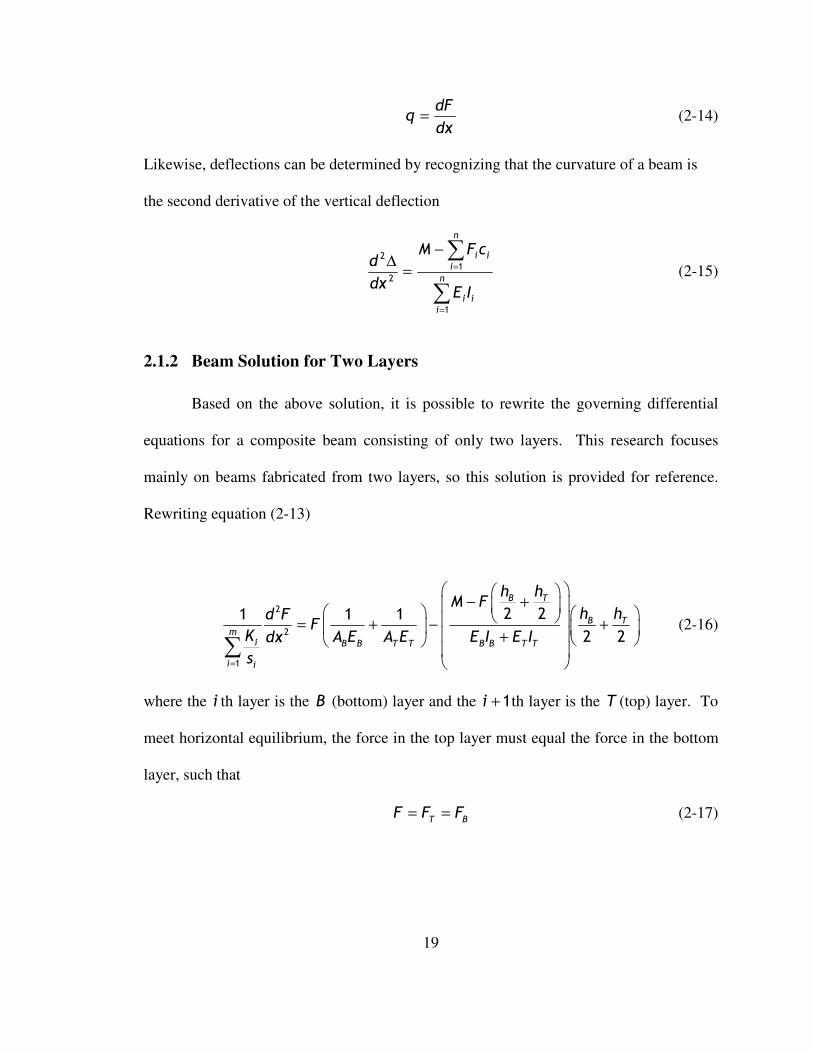
2.1.2 Beam Solution for Two Layers
Based on the above solution, it is possible to rewrite the governing differential
equations for a composite beam consisting of only two layers. This research focuses
mainly on beams fabricated from two layers, so this solution is provided for reference.
Rewriting equation (2-13)
2
2
1
2 21 1 1
2 2
B T
B T
mi B B T T B B T T
i i
h hM F
h hd FF
K A E A E E I E Idx
s=
− + = + − + +
∑ (2-16)
where the i th layer is the B (bottom) layer and the 1i + th layer is the T (top) layer. To
meet horizontal equilibrium, the force in the top layer must equal the force in the bottom
layer, such that
T B
F F F= = (2-17)

20
By recognizing that E , I , A , h , and K
s∑ are constants for each layer, we can introduce
two new constants that are similar in form to those proposed by Newmark, Seiss, and
Viest (1951)
2
1
2 21 1B T
mi
Fi i B B T T B B T T
h h
KC
s A E A E E I E I=
+ = + + +
∑ (2-18)
1
2 2B T
mi
Mi i B B T T
h hK
Cs E I E I=
+
= +
∑ (2-19)
Therefore, we can rewrite equation (2-16) in a much simpler form
2
2 F M
d FC F C M
dx− = − (2-20)
Since both F and M are functions of x , equation (2-20) is a standard ordinary
differential equation. For a given loading (moment) function, along with material and
section properties, a specific solution can be determined for the axial force F in the
layers at any point. With the use of equation (2-15), it is also possible to directly solve
for the displacement at any point along the length of the beam.
2.1.3 Beam Solution for Three Layers
The following calculations are based on a simplified three-layer beam, such that
the modulus of elasticity, E , is identical in all three layers, as well as each layer has the
same cross sectional properties (i.e., b and h are identical for each layer). The solution

21
of the interlayer slip for a three-layer beam with varying material or sectional properties
could be found using the procedure discussed below.
With three identical layers in the built-up beam, the middle layer will not
experience any cumulative axial force. Also, the forces in the top and bottom layers will
be identical. With this in mind, it is possible to write equation (2-13)
as
2
2,
1 ,
1 2( )
3mi l
l i l
d F F M Fhh
K AE EIdx
s=
− = −
∑ (2-21)
which is the governing differential equation describing the axial force, F at any point
along the layer’s length. Equation (2-21) can be simplified and rewritten as
2
3 32 F M
d FC F C M
dx− = − (2-22)
where 3F
C and 3M
C are constants that are calculated as
2
31
1 2
3
ml
Fl l
K hC
s AE EI=
= +
∑ (2-23)
3
1
2
3
ml
Fl l
K hC
s EI=
=
∑ (2-24)
Recognizing that both A and I can be written in terms of b and h , these constants
simplify to
3
1
9ml
Fl l
KC
s bhE=
=
∑ (2-25)
3 2
1
4ml
Ml l
KC
s bh E=
=
∑ (2-26)

22
The deflection at any point along the beam can be found by using equation (2-15), which
reduces to
2
2
2
3
d M Fh
EIdx
∆ −= (2-27)
for a built-up beam consisting of three identical layers.
The solution of the differential equation for a three-layer beam, shown in equation
(2-22), with a specific loading configuration (point loads at any point, symmetrically
placed point loads, or a uniformly distributed load), will be identical to those developed
for a two-layer beam. In order to use the two-layer solutions, 3F
C and 3M
C must be
substituted for F
C and M
C , and the three-layer built-up beam must be made from three
identical layers with identical shear key configurations.
2.2 Solutions for the Two Layer Model with Uniform Loading
2.2.1 Axial Force in Each Layer
For a uniformly distributed load w on a simply supported beam of length L , we
can write the moment equation for any point along its length x as
( )( )2
wxM x L x= − (2-28)
which can be substituted into equation (2-20). Solving for ( )F x
2
1 2 2
(2 )( )
2F FC x C x M F F
F
wC xLC x CF x C e C e
C
− − += + − (2-29)

23
where 1
C and 2
C are integration constants. There cannot be an axial force in the layers at
the ends of the beam, so (0) 0F = and ( ) 0F L = . Using these boundary conditions,
1C and
2C can be determined as
( )
( )1
2
1 F
F F
C L
M
C L C L
F
wC eC
C e e−
−=
−
( )
( )2
2
1F
F F
C L
M
C L C L
F
wC eC
C e e
−
−
−=
− (2-30)
Substituting these integration constants back into equation (2-29) results in
( )( )( )
( )2
sinh ( )( ) cosh 1 cosh 1
2sinh
FM F
F F
F F
C xwC C x L xF x C x C L
C C L
− = + − − +
(2-31)
The shear flow at any point of the beam can be determined by solving equation (2-14).
Likewise, determining the deflection at any point along the length can be found using
equation (2-15), recognizing the boundary conditions of (0) 0∆ = and ( ) 0.L∆ =
Solutions for the shear flow and deflection at any point can be found in Appendix A.
2.2.2 Bounds on Uniformly Distributed Load Solution
The lower bound for the axial forces in each layer, caused by composite action in
a beam with partial interaction, should be the same as a simple stacked non-composite
beam. Likewise, the upper bound for the axial forces for a beam with partial interaction

24
should be the full depth beam with no interlayer slip. The amount of interaction
between the two layers is directly proportional to the stiffness of the individual shear
keys, K . The lower bound is thus
0
lim ( ) 0k
F x→
= (2-32)
If we assume the top and bottom layers have the same breadth, the upper bound can be
found to be
3 ( )
lim ( )
82 2
kB T
wx L xF x
h h→∞
−=
+
(2-33)
At the midspan of the beam, 2
Lx = , which results in
23
232
2 2B T
L wLF
h h
= +
(2-34)
The axial force in the top or bottom half of a full composite section of width b is
( )2
Mc bcF x
I
=
(2-35)
where c is the distance from the neutral axis to the extreme fibers. We can rewrite
equation (2-35) as
( )3
2 2 2 2 2( )
2
2 2
12
B T B T
B T
h h h hwxL x b
F xh h
b
− + +
=
+
(2-36)

25
Again looking at midspan where 2
Lx =
23
232
2 2B T
L wLF
h h
= +
(2-37)
which is the same as equation (2-34). Thus, the solution for the axial force in a partially
composite beam subjected to a uniformly distributed load matches the required bounds.
2.3 Other Loading Conditions
Solutions of the interlayer slip model for a single point load at any point on a
simply supported beam were developed, as well as the solution for a pair of point loads
symmetrically placed on a simple beam. These derivations and formulae can be found in
Appendix B and Appendix C, respectively.
2.3.1 Numerical Integration
Solutions of the interlayer-slip equations become quite difficult when modeling
complex distributed loadings, either those that vary linearly or by some varying rate
along the length of the beam. The solution to a point load at any location, along with a
numerical integration technique, such as Newmark’s method (Newmark, 1959), makes it
possible to accurately model the more complex distributed loads without additional
solutions of the interlayer slip model.
2.3.2 Linear-Elasticity and Superpositioning
The development of the general interlayer slip theory was based on the
assumption of linear-elastic behavior. With linear-elastic behavior, it is possible to use

26
superpositioning to model complex structures by adding the effects of individual loads.
To show that this method indeed works for the interlayer slip model, the solution for a
two-layer beam with two point loads symmetrically placed was developed. The solution
can be found in Appendix C. The deflection of the two-point load condition was
compared to a superimposed single-point load condition, as is shown in Figure 2-5.
In order to behave linear-elastically, the deflection at any location on a beam
subjected to two point loads must be the same as the combination of the respective
deflections caused by a single point load. An arbitrary beam and symmetric point
loading configuration was analyzed, both using superposition of the single point load
solutions as well as by using the two symmetrically placed point load solution. The
resultant deflected shapes, as well as plots of axial force at any point along the length,
were identical.

27
∆1
∆2
∆1 + ∆2
Figure 2-5 Superpositioning of pointloads

28
2.4 Stress Distribution
The strain distribution at any point in a layer of a two-layer partially composite
beam, described in section 2.1.1 as equation (2-7), can be written as
T TT
T T T T
M z F
E I A Eε = − (2-38)
B BB
B B B B
M z F
E I A Eε = − − (2-39)
where the subscripts T and B represent the top and bottom layers, respectively, and z is
the distance from the center of the layer to the point of interest. Using Hooke’s law
(equation (2-4)), the stress in each layer is
TT
T T
M z F
I Aσ = − (2-40)
BB
B B
M z F
I Aσ = − − (2-41)
where the first term represents the bending stress in the layer, and the second term
represents the axial stress induced from the partial composite action. Again assuming the
same curvature in both layers, as described by equation (2-12), the original moment in the
top and bottom layers (T
M and B
M ) can be related to the total applied moment M in the
built-up beam as
T B
T T B B T T B B
M M M Fc
E I E I E I E I
−= =
+ (2-42)
This relationship can be used to write the stress equations (2-40) and (2-41) in terms of
the total applied moment and the axial force in any layer, such that

29
( ) T
T
T T B B T
M Fc E z F
E I E I Aσ
−= −
+ (2-43)
( ) B
B
T T B B B
M Fc E z F
E I E I Aσ
−= − +
+ (2-44)
These stress equations can be evaluated for a beam with a specific loading configuration
by solving the interlayer slip model, described in section 2.1, for the axial force in each
layer.
The lower and upper bounds on the stress equations (2-43) and (2-44) must match
the maximum stress in simple stacked and full depth beams, respectively. To verify these
limits, the stress in an arbitrary beam with symmetrically placed point loads was
analyzed. The amount of interaction between layers was varied from no interaction (full
slip) to full interaction (no slip) by adjusting the stiffness of the shear key, K , shown in
equations (2-18) and (2-19). As 0K → , the calculated extreme fiber stress in the beam
using the interlayer slip model approached the extreme fiber stresses in a pair of simple
stacked beams with the same applied load. Likewise, as K → ∞ , the calculated extreme
fiber stress in the beam using the interlayer slip model approached that of a full depth
beam. For any specific applied load, the extreme fiber stress in a simple stacked beam
will be exactly twice that of full depth beam.
The magnitude of maximum stress along the length of a beam may be different
for a built-up beam with partial composite action than for a full depth or simple stacked
beam, depending on the applied loading configuration. The stress in a full depth or
simple stacked beam is a function of the moment and cross-sectional properties (distance
to point of interest and the moment of inertia), and assuming a constant cross-section

30
along the length, the shape of the moment diagram is the shape of the extreme fiber
bending stress diagram. For a built-up beam, the change in axial force in the layers due
to partial interaction can result in localized points of maximum stress. Figure 2-6 shows
the normal stress distribution at the beam face for an arbitrary built up beam with some
interlayer slip (solid line) and a full depth solid beam (dashed line), subjected to two
symmetrically placed point loads. Peaks in the stress diagram are noticeable in the built
up beam at the points of applied load.
Figure 2-6 Normal stress diagrams for an arbitrary full depth (dashed line) and built up (solid line)
beam
2.5 Shear Keys
The closed-form interlayer slip solutions previously developed require knowledge
of the stiffness of each particular connector along the beam length (see Figure 2-7).
These connector stiffnesses depend on the type and configuration of the shear key as well
as the beam material properties. From this point onward, the term “shear key” includes
the actual wood key along with the clamping connectors, behaving as an assembly.

31
Two configurations of shear keys are common in traditional timber design; one is
a key inclined to the interface and the other is a key square to the interface. Both consist
of a pair of wedges, driven in from opposite faces of the timber, to ensure a tight fitting
joint. These wedges will form a shear key that will then be installed either square to the
timber or at an incline. Fabricating the notch for the square shear keys requires slightly
less effort, but parallel to grain shearing of the wedges will become a design concern.
Notches for the inclined wedges may be slightly more difficult to cut, but the key will be
almost entirely in compression, greatly reducing concerns about horizontal shearing of
the keys. The inclined shear key reduces the angle to the grain of the re-entrant corner of
the notch, which will likely have an effect at reducing the stress concentration at this
point.
As force is transmitted through an inclined shear key, it will cause the shear key
to rotate and thus open up a gap at the interface. A mechanical connector, either a
through bolt, lag bolt, or other screw, is required to provide a clamping force. This
connector will be loaded in shear at the interface as well, and thus can contribute to the
overall stiffness of the interface. Axial stretching of the connector will likewise cause
some movement of the shear key, and thus this stiffness also needs to be included in
determining the stiffness of the interface. The square and inclined shear keys can be seen
in Figure 2-7.

32
(a) (b)
(c)
Figure 2-7 Side view of (a) square and (b) inclined shear keys along with (c) a top view showing the
wedge shape of the shear keys
2.5.1 Shear Key Stiffness
Shear keys are used to inhibit slipping between the layers of a built up beam.
Thus, the stiffness of the shear keys in this plane is of particular concern in determining
the strength and efficiency of the built-up beam, where efficiency is defined as the
percentage of a comparative solid-sawn beams horizontal shear that is resisted (see 2.6).
We will start with an inclined shear key notched to a deptht into the individual layers and
of length w , as shown in Figure 2-8. In Figure 2-8, N is the horizontal force that the
shear key is resisting, and R is the clamping force required to counteract the rotation of
the keys. P is the axial force, which is components of N and R , acting parallel to the
shear key.

33
Figure 2-8 Inclined shear key
As axial force is developed in the individual layers, the shear key will deform as shown
in Figure 2-9. As was already noted, the horizontal movement of the key is of primary
concern. Contributions to this movement include compression of the timbers at the
notches, axial shortening of the shear key, and the gap created as the key rotates.
Figure 2-9 Deformed inclined key
In order to model the stiffness of the shear key, we can depict the shear key shown in
Figure 2-8 as a series of three springs which are shown in Figure 2-10. The B
K and T
K
θ
N
P
R
P
N
R
w
t

34
terms represent the stiffnesses in compression of the beams in the bottom and top
members. The K
K term represents the axial stiffness of the shear key.
w
t
P
KB
KTKK
Figure 2-10 Springs-in-series model of the shear key
The effective stiffness of the shear key connection, eff
K is
1 1 1 1
eff B K TK K K K
= + + (2-45)
With the assumption that the top and bottom timbers are of similar properties, T B
K K= ,
we can solve for the effective stiffness as
2
K Teff
K T
K KK
K K=
+ (2-46)
The total compressive displacement of the keyed connection can be written as
comp
eff
P
K∆ = (2-47)
We are concerned with the displacement oriented parallel to the timbers, not oriented
parallel to the keyed connection. From Figure 2-8, we can see P has a horizontal
component N , and compressive displacement comp
∆ has a horizontal displacement key
∆ ,
which allows us to write

35
key
eff
N
K∆ = (2-48)
The axial stretching of the clamping connectors also contributes to the slipping between
the layers, as it allows the key to rotate slightly. The axial displacement of the clamping
connectors, stretch
∆ , is written as
stretch
clamp
R
K∆ = (2-49)
where clamp
K is the axial stiffness of the clamping connector (see Figure 2-11). If multiple
screws or bolts are used to provide the clamping force, clamp
K is the summation of the
cumulative axial stiffnesses.
Figure 2-11 Displacement components of a shear key
Again from Figure 2-8, we can see the forces R and N are components of P , thus
tanR N θ= . The horizontal slipping clamp
∆ caused by the axial stretching of the
∆ key
∆ stretch
t
2t
t

36
clamping connector can also be written as tanclamp stretch
θ∆ = ∆ . The horizontal
displacement caused by the axial stretching of the clamping connector can thus be written
as
2tan
clamp
clamp
N
K
θ∆ = (2-50)
Combining the horizontal displacement from the axial compression of the key component
as well as the horizontal displacement from the axial stretching of the clamping
connector, we are able to write the stiffness for a single shear key as
key
key clamp
NK =
∆ + ∆ (2-51)
Substituting equations (2-48) and (2-50) into equation (2-51), the stiffness of a shear key
can be written as
2tan
clamp eff
key
clamp eff
K KK
K K θ=
+ (2-52)
The key stiffness shown in equation (2-52) ignored the stiffness contribution for the
clamping connectors loading in shear. For most connectors, consisting of screws or bolts,
the stiffness of a laterally loaded connection is assumed to be proportionally very low and
is therefore ignored in this analysis. This assumption is later verified in section 4.5.
2.5.2 Shear Key Stiffness Coefficients
In order to calculate the shear key assembly stiffness for use in the interlayer slip model,
the various stiffness components in equation (2-52) need to be calculated. With the width

37
of the timber beams being b , and the depth of influence in the compression zone of the
timber L , being approximated as two times the key thickness t using a Boussinesq / soil
pressure bulb analogy (Coduto, 2001) (see Figure 2-11), the stiffness of the timbers being
compressed at the shear key interface is
2 2
T
AE tbE bEK
L tθ θ θ= = = (2-53)
where Eθ is the modulus of elasticity of the timber at an angle θ to the grain, as shown in
Figure 2-8. Eθ can be approximated by the use of Hankinson’s formula, such that
2 2sin cos
E EE
E Eθ
θ θ⊥
⊥
=+
�
�
(2-54)
Published values for the modulus of elasticity for timber are values parallel to the grain.
Perpendicular to the grain modulus values for wood are seldom measured or recorded.
Instead, elastic ratios are commonly used that relate the longitudinal modulus (parallel to
grain) to radial and tangential modulii (perpendicular to grain). The elastic ratios are
published values relating one orthotropic material modulus to that of another. These
elastic ratios vary widely depending on species and grain orientation, with tangential to
longitudinal ratios as low as 0.02 and radial to longitudinal ratios as high as 0.197 (FPL,
1999). The elastic ratios have been shown to vary with a positive correlation to the
longitudinal modulus of elasticity (Bodig and Jayne, 1982). Several authors suggest
averaging the elastic ratio between the radial and tangential directions, as this grain
orientation is seldom known at the time of design (Bodig and Jayne, 1982; Wangaard,
1981). These authors also suggest using an elastic ratio on the order of 1:20 (that is,
20E E⊥=�
). Their recommendation is based on the predominant use of softwoods in

38
design. For this research, and in common heavy timber construction practice, white oak
keys were used, which has elastic ratios of 1:14 (longitudinal to tangential) and 1:6
(longitudinal to radial) (FPL, 1999). Yellow poplar has published ratios of 1:24 and 1:10,
respectively. Based on these values, the elastic ratio of 1:12 was initially chosen to relate
the longitudinal and perpendicular modulii ( 12E E⊥=�
). We can rewrite equation (2-54)
to include this as
212 11cos
EEθ
θ=
−
� (2-55)
Including equation (2-55) into the timber stiffness equation (2-53) yields
22(12 11cos )
TIMBER
T
bEK
θ=
−
�
(2-56)
Likewise, the stiffness for the key portion is
2(12 11cos )
KEY
k
btEAEK
L wϕ= =
−
�
(2-57)
where ϕ is the orientation of the shear key grain with respect to the force P .
The stiffness of the clamping connectors may be able to be approximated using a
mechanics based approach as above if a through-bolt or other similar type of connector is
used. When screws are used, the axial stiffness will need to be verified from physical
tests or manufacturer’s data, as no method to calculate the axial withdrawal stiffness of a
screw is known to exist.

39
2.6 Beam Efficiency
The efficiency of a built-up beam is directly related to the amount of interaction
between the layers. The interaction results in axial forces in each layer (see Figure 2-3).
A low efficiency beam has little interaction between the layers (acts like a simple-stacked
beam) and small additional axial forces in each layer. A high efficiency beam has nearly
rigid interaction between the layers (acts like a full-depth beam). The rate of change of
the axial force in the layers is the shear flow (see equation (2-14)). The shear flow in a
transversely loaded full depth solid beam is calculated as
VQ
qI
= (2-58)
where V is the vertical shear, Q is the first moment, and I is the moment of inertia.
Plots of the shear flow in both an arbitrary built-up beam as well as a full depth beams are
shown in Figure 2-12a and Figure 2-12b. The shape of the shear flow diagrams for a
beam subjected to a uniformly distributed load appears quite similar regardless whether it
is a full depth beam or a built-up beam. A beam subjected to a pair of concentrated
points load exhibits substantial variation in the respective shear flow diagrams near the
center of the span. In either loading case, the area under the built-up beam shear flow
diagram is less than the area under the full-depth beam diagram.

40
(a)
(b)
Figure 2-12 Shear flow in partially composite beams subjected to (a) two concentrated loads and (b)
a uniformly distributed load.
The area under the shear flow diagrams is the axial force generated in each layer
of the built-up beam. The ratio of the area under a built up beam shear flow diagram to
the area under an equivalent full depth beam represents the beam efficiency λ , such that
dFdx
dxVQ
dxI
λ =∫
∫ (2-59)
Full Depth Beam Built Up Beam

41
where the first moment Q and moment of inertia I are based on the full depth cross-
section. The value of λ can range between zero and one.

42
3 Physical Testing Overview
In order to verify the interlayer slip model and shear key stiffness components
developed in the previous section, physical testing was conducted on individual, small
scale components as well as full sized beams. To best utilize the materials available for
the testing, configurations that were similar to those being used in professional practice
were used (Brungraber, 2008). These configurations are further described below.
3.1 Timber and Key Species
3.1.1 Timber Species Selection
According to the Timber Frame Business Council, there are several species
commonly used in timber frame construction: Douglas fir, eastern white pine, southern
yellow pine, and red oak (TFBC, 2009). While each of these common species have
specific strong points, yellow poplar (Liriodendron tulipifera) was chosen for this
research. Yellow poplar is a commonly available, inexpensive, fast-growing hardwood
that has reasonable structural qualities. There is also a longstanding history of yellow
poplar use in timber structures, including covered bridges and mill buildings (Forest
Service, 1985).
Yellow poplar was selected primarily because of the availability of large, clear,
straight grained specimens. Clear specimens were desired so that natural defects such as
knots would not dominate behavior during the physical testing. Yellow poplar timbers
were readily available from a sawmill within Michigan which further added to the appeal

43
of their use. An increasing availability of second-growth yellow poplar (Forest Service,
1985) was also a contributing factor in its selection.
3.1.2 Shear Key Species Selection
Traditional and contemporary sources suggest using hardwoods, in particular
white oak (Quercus alba), for wedge stock (Kidwell, 1898; Karlsen, 1967). According to
section 1.6.3 of the TFEC 1-07 Standard for Design of Timber Frame Structures and
Commentary (TFEC, 2007):
Wood wedges used to secure through-tenons or scarf joints, or used for other
structural applications shall be fabricated from clear, straight-grain, defect-free,
hardwood stock. Wedges shall be fabricated to minimize slope of grain, but in no
case shall slope of grain be greater than 1:6 relative to each face of the wedge.
The specific gravity of the wedge stock shall not be less than that of the timber
used in the connection, but in no case shall the oven-dry specific gravity of the
wedge stock be less than 0.57.
The shear keys are acting in a structural application and consist of a pair of wedges,
therefore the requirements set forth in TFEC 1-07 above should directly apply. As there
was substantial agreement between all of the investigated sources, white oak was chosen
as the main shear key material.
A non-traditional manufactured shear key material was also desired for use with
the key testing. Manufactured shear key material considered for possible use included
glue-laminated timbers, laminated veneer lumber (LVL), and parallel strand lumber

44
(PSL). These manufactured wood products appeared to have several advantages over the
white oak for use as shear keys, mainly that they:
- are thoroughly dried. Any shrinkage in a shear key would greatly reduce
the efficiency of the keyed beam.
- have interwoven or discontinuous grain. Seasoning and growth defects
are removed or broken up by the manufacturing process, decreasing the
likelihood of damage during installation.
- have higher and more consistent modulus of elasticities than solid-sawn
material. The manufacturing process culls low grade material from the
final product, and adhesives used to bind the wood fibers increases the
stiffness.
The main deterrents from using manufactured wood products for the shear key material
are that they:
- can cost significantly more than solid-sawn pieces of white oak.
- are commonly available only in several species.
- use adhesives in the manufacturing process. One of the main
contemporary uses of keyed beams is in places were adhesives are not
desired.
Glulams, while thoroughly dried, still regularly use large pieces of continuous
wood (although finger jointing allows for shorter pieces to be used), and are one of the
building materials keyed beams are intended to replace. Laminated veneer lumber is
commonly available only in narrow thicknesses (typically 1.75 inch or less), limiting the
size of shear keys. Parallel strand lumber can be made into almost any size, and because

45
of the fabrication process, is considerably stiffer when loaded parallel to the grain than
solid-sawn material.
Based on the above factors, parallel strand lumber was chosen as the
manufactured wood product to be used as shear keys, specifically southern pine TrusJoist
2.0E Parallam PSL (Parallam). Parallam PSL is described as being “manufactured from
strands of a single wood species, or species combinations, that are oriented parallel to the
length of the member and coated with a phenol-formaldehyde adhesive.” (ICC-ES, 2007).
3.2 Key Configuration
3.2.1 Key Orientation
Stiffness models were developed for both keys inclined to the interface of the
timbers (inclined keys) and keys square with the interface (square keys). Kidwell (1898)
argued that notches for the inclined keys were more difficult to cut and that the inclined
keys were quite prone to roll and force the layers apart. He therefore recommended
square keys. Karlsen (1967) instead argued that square keys are prone to shearing along
the grain and thus preferred inclined keys which act primarily in compression.
With the availability of modern power tools, notching for an inclined key is no
more difficult than notching for a square key. Likewise, the stiffness model for the keys
includes rotation of the key, so any propensity of one key configuration to roll compared
to the other can be directly accounted for. Shearing parallel-to-the-grain of the key is a
legitimate concern with the square keys. Parallel-to-the-grain shear failures are a sudden
and brittle failure.
46
An additional benefit of the inclined keys is they require removal of less material
from the timbers than an equivalent capacity square key. An inclined key also results in a
smaller stress concentration at the re-entrant corner of the notch, since the notch
orientation is rotated slightly (Karlsen 1967). An inclined key’s ability to resist only one-
way shear (reversal of moment in the keyed beam can result in reversal of slip directions)
can be seen as a deterrent for its use. However, the difficulty in fabricating a square key
that can carry two-way shear without allowing some initial slipping makes this argument
impractical. Based on these reasons, only inclined keys are investigated in this research’s
physical testing components.
3.2.2 Grain Direction
Physical behavior, which is also evident in the analytical model previously
developed, shows the stiffness of the shear keys directly impacts the stiffness of the
keyed beam. For wood shear keys, the parallel-to-the-grain modulus of elasticity is
approximately ten to twenty times as stiff as the perpendicular-to-grain modulus of
elasticity (FPL, 1999). Orienting the shear keys so that they are compressed parallel-to-
the-grain would therefore result in a stiffer keyed beam.
Kidwell (1898) acknowledged wood is stiffer parallel-to-grain than perpendicular-
to-grain, but still advocated that the wedge stock be installed so that it is loaded in the
perpendicular-to-grain direction. “The writer does not believe that there is any solid
foundation for the idea that the grain of the keys should be vertical. This would greatly
increase the cost of making the keys, and probably result in causing many of them to split

47
while driving.” (Kidwell, 1898). Kidwell went on to discount all wooden keys and
suggested using only cast-iron ones because of their much higher modulus of elasticity.
Karlsen (1968) acknowledged that connections with keys loaded in compression
perpendicular-to-the-grain are much easier to fabricate and install, but disliked their use
because of their low stiffness. He claimed shear keys loaded in a parallel-to-the-grain
fashion will be much stiffer, although they cannot be installed as wedges due to splitting
during installation, and instead must be installed as solid pieces of wood. However,
Karlsen also suggested parallel-to-grain shear keys end up having no greater capacity
than perpendicular-to-the-grain keys. The failure to carry more load, despite being
considerably stiffer, is purportedly because they cannot be made to carry load evenly due
to fabrication tolerances. According to Karlsen, the uneven load carrying results in high
stress concentrations at notch corners, which in turn cause some connections to fail
before others even start to carry load (Karlsen, 1968).
An attempt was made to verify Kidwell’s and Karlsen’s comments about parallel-
to-the-grain wedges splitting during installation. Three pairs of straight grained,
unchecked, white oak wedges, 2.5 inches thick, 10 inches long, and 8 inches in combined
depth were fabricated with the grain running approximately perpendicular to the wedge
faces (Figure 3-1). The pairs of wedges were installed into a similar sized inclined
notches in a keyed beam. The wedges were driven with a 3-lb drill hammer to fully
engage both bearing faces. Of the three sets of wedges, one set was able to be installed
fully with no splitting, while at least one wedge from the each of the other two sets split
along the grain during the driving process (Figure 3-2).

48
1
10
3"
2"
10"
10"
412"
312"
312"
412"
1
10
Figure 3-1 2.5 inch thick shear key wedge dimensions
Figure 3-2 Solid sawn parallel-to-the-grain wedges are prone to splitting during installation
With convincing evidence that solid sawn parallel-to-grain wedges were not
feasible, the research instead focuses on using white oak wedges as shear keys installed
with the load orientated perpendicular to the shear key grain. Due to the fabrication
process used in making Parallam PSL, the shear keys using this material were able to be
installed as wedged shear keys with the grain running parallel to the load direction.
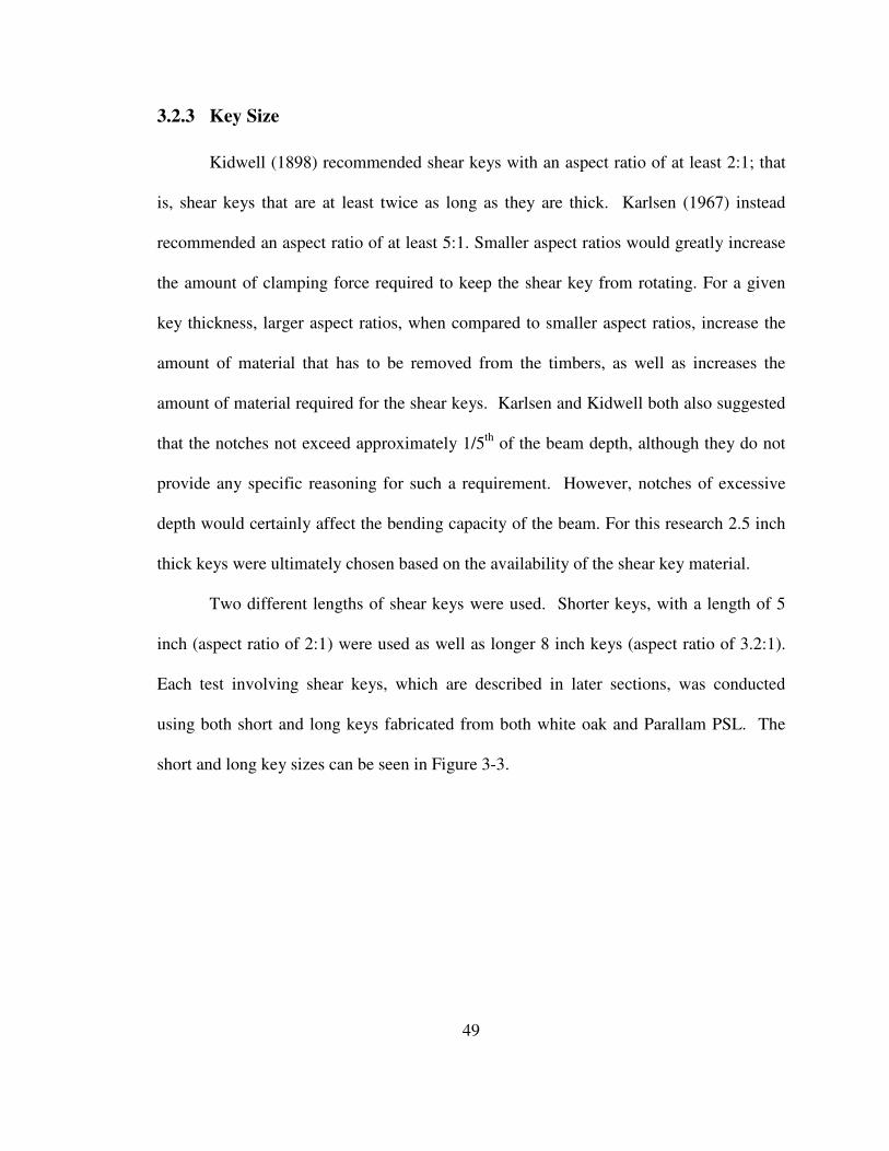
49
3.2.3 Key Size
Kidwell (1898) recommended shear keys with an aspect ratio of at least 2:1; that
is, shear keys that are at least twice as long as they are thick. Karlsen (1967) instead
recommended an aspect ratio of at least 5:1. Smaller aspect ratios would greatly increase
the amount of clamping force required to keep the shear key from rotating. For a given
key thickness, larger aspect ratios, when compared to smaller aspect ratios, increase the
amount of material that has to be removed from the timbers, as well as increases the
amount of material required for the shear keys. Karlsen and Kidwell both also suggested
that the notches not exceed approximately 1/5th
of the beam depth, although they do not
provide any specific reasoning for such a requirement. However, notches of excessive
depth would certainly affect the bending capacity of the beam. For this research 2.5 inch
thick keys were ultimately chosen based on the availability of the shear key material.
Two different lengths of shear keys were used. Shorter keys, with a length of 5
inch (aspect ratio of 2:1) were used as well as longer 8 inch keys (aspect ratio of 3.2:1).
Each test involving shear keys, which are described in later sections, was conducted
using both short and long keys fabricated from both white oak and Parallam PSL. The
short and long key sizes can be seen in Figure 3-3.

50
212"
8"
17.4°
(a)
212"5"
26.6°
(b)
Figure 3-3 (a) Long and (b) short shear key configurations
3.2.4 Wedge Slope
The shear keys used in this testing consisted of a pair of inclined wedges cut from
a single piece of material. The incline allows the shear key (pair of wedges) length to be
fine tuned, once installed into the notched timbers, to ensure full contact across all
bearing faces. The axial force P being resisted by the shear key must be transferred
across the interface between the wedges as a normal force N
P . A friction force F
P is
thereby required to keep the wedges in place as they are loaded in compression (Figure
3-4). The static friction coefficient S
µ for wood varies based on moisture content,
smoothness of the surfaces, species, and other variables, although the Wood Handbook
lists a range 0.3 0.5S
µ = − (FPL, 1999). These friction coefficients of 0.3 to 0.5 would
permit any rise under 3 to 5 to maintain equilibrium. Per section 1.6.3 of the TFEC 1-07,
which is shown above in section 3.1.2, the slope of a wedge must not exceed 1:6
(1.67:10). With this in mind, a conservative slope of 1:10 was chosen for the wedges
used to form a shear key.

51
P
PN
PF
10
RISE
Figure 3-4 Forces acting on a pair of wedges
3.3 Clamping Connectors
3.3.1 Connector Type
As force is applied to the shear keys, whether they are inclined keys or square
keys, the keys will have a tendency to rotate (Figure 2-9). Mechanical connectors are
used to resist this rotation. Several various options were investigated for potential use as
clamps. These include:
- Through bolts. Through bolts consist of machine bolts installed
orthogonally to the slip interface, through the entire depth of the timbers
and secured with a nut and washer. Through bolts require drilling holes
through the beams, reducing their net cross section. For framing to sit
directly on the top face of the keyed beam, through bolts would need to be
countersunk into washer pockets, further reducing the net section. The
bolt head and washer would also be left visible on the bottom face of the
52
beam. As most timber beams have their bottom face exposed as a finished
surface, visible bolts could deter from the aesthetic appeal.
- Lag bolts. Lag bolts, like through bolts, would require drilling holes in the
timbers and reducing their net cross section. Lag bolts could be installed
entirely from the top (hidden face) and thus would be much less visible,
but would still require countersinking. Installation of lags also requires
the use of impact drivers.
- Continuously threaded screws. Screws that are threaded along the entire
length are commonly used for radially reinforcement of curved glulam
timbers. Unlike bolts or lags, they do not require pre-drilling, and they
also interrupt considerably less grain. Screws can also self counter-sink.
- Dual threaded screws. Dual threaded screws are much like continuously
threaded screws, however, they are threaded with slightly different pitches
on an upper and lower portion of the shaft. As they are installed, the
variance in pitch causes the middle of the screw to be axially pre-
tensioned, drawing the two connecting timbers together.
In order to increase the rate and ease of fabrication, as well as limit the reductions made
to the cross section of the timbers, screws were chosen to provide the clamping action
required at the shear keys. OMG Fastenmaster Double Thread LogHog (Figure 3-5)
screws were ultimately chosen from the various manufacturers due to their long-standing
history in the timber framing market.

53
Figure 3-5 Double threaded log screw
3.3.2 Connector Placement
The placement of the connectors used to resist the rotation of the shear keys will
directly determine the quantity of connectors required. As the distance from the shear
key increases, the moment arm between the point of rotation and the connector increases,
decreasing the capacity. However, excessive distance between the shear key and
connector can result in bending of the individual timber layers, so a balance must be
maintained. For ease of fabrication, the clamping fasteners were placed 2 inch from the
center of the key’s bearing area. See Figure 3-6.
2" 2"
18"1634" 18"
Figure 3-6 Key placement and screw location on keyed beams used in the full-scale testing
3.3.3 Connector Quantity
While previous authors provided recommendations for the clamping force
required to secure joints, a mechanics-based approach was instead used for this research.
The placement and number of screws required to adequately clamp each key was

54
determined after the key configurations were developed. The clamping required for the
shear key configuration shown in Figure 3-3 (a), with white oak keys installed such that
they are loaded perpendicular to grain, was calculated. Calculations can be found in
Appendix D. A total of four LogHog screws (two pairs of two) were required to clamp
each shear key. The governing compressive force in the key was determined from the
cross-grain compressive capacity of the white oak shear key at the proportional limit. A
similar clamping configuration was then used for all other shear key configurations.
3.4 Beam Size
The interlayer slip model and shear key stiffness model permit any sized beam to
be used. Therefore, a timber size was chosen based on common practice and the
availability of materials. Cross sectional dimensions are normally specified to the nearest
two inch nominal increment (e.g., 6 inch by 6 inch nominal, 8 inch by 8 inch nominal)
with lengths specified to the nearest two-foot increment (AF&PA,2005). The
International Building Code (IBC) specifies timber cross sections must be at least 6
inches or 8 inches depending on their use in a structure to meet the classification of heavy
timber (ICC, 2006). In order to incorporate all categories within the IBC heavy timber
category, nominal 8 inch by 8 inch timbers were chosen. Based on the log inventory of
the sawmill providing the timbers for the research, the maximum length of timbers was
set at 14 feet.

55
3.5 Loading Configuration
A primary focus of the research was to predict actual keyed beam behavior using
the theoretical interlayer slip model and shear key stiffness parameters developed in the
previous section. For static load tests on simply supported full sized members, ASTM
D198 provides guidance for the proper testing and loading procedure (ASTM, 2007). Per
ASTM D198, two symmetric point loads should be placed at third-points on the beam,
although other placements are permitted for special purposes. This loading configuration
creates a constant shear, linear moment distribution in the ends of the beam, with a zero
shear, constant moment distribution in the middle section.
ASTM D198 also provides guidance for determining the over-all length of the
beam as
R
MAX
Sa
hφ
τ= (3-1)
where a is the distance from the end support to the nearest point load, h is the total
depth of the beam, R
S is the published average modulus of rupture for the material, and
MAXτ is the average maximum shear stress. φ is an adjustment factor with a suggested
range of 0.4 to 0.6 (ASTM, 2007). For a two layer beam fabricated from nominal 8 inch
by 8 inch (7.5 inch by 7.5 inch approximate actual size) material, the beam depth will be
15 inches. Values published in the Wood Handbook for yellow poplar are 10,100 psi
and 1,190 psi for modulus of rupture and shear stress, respectively (FPL, 1999). Using
an adjustment factor φ of 0.5, the distance from the end support to the point load was
calculated as 63.7 inches, and truncated to 63 inches for simplicity. With 14-foot timber

56
material, and accounting for three inches of bearing and overhang on each end, this
results in a 36 inch spacing of the point loads at the center of the beam. ASTM D198
recommends equal spacing for the end and center sections, using a shorter center distance
increases the length of the constant shear sections, which are the areas of particular
concern in this research (ASTM, 2007). The loading configuration, along with the shear
and moment diagrams, are shown in Figure 3-7.
Figure 3-7 Loading configuration for full scale beam testing
a = 63" 36" a = 63" 162"
P P
SHEAR
MOMENT
Vmax=P
P Mmax=Pa
h = 15"

57
3.6 Key Layout in Keyed Beam
In order to achieve full interaction (no slip allowed between the layers) in a two-
ply keyed beam using the loading configuration shown in Figure 3-7, all of the horizontal
shear developed in a full depth beam must be resisted by the shear keys. The minimum
spacing between shear keys is limited by the shear strength parallel to grain of the
timbers between each shear key. The maximum spacing between shear keys is limited by
the shear flow that each key needs to resist. As slippage between layers will occur in the
actual beams, using the interlayer slip model to develop the maximum shear key spacing
would be most appropriate. The method used in this section was an approximation to
ensure the testing configuration was reasonable.
The minimum spacing between shear keys, MIN
s , is limited by a block shear
failure of the timber between keys, and was calculated by
0.95
2MIN
V
Ps
b F= (3-2)
where P is the cross-grain compressive strength of the shear key at the proportional limit
(16,050-lb per Appendix D), b is the timber width (7.5 inch), and 0.95V
F is the 95%
inclusion value (5% exclusion) of the shear stress parallel to grain for unseasoned yellow
poplar (Figure 3-8). A 95% inclusion limit was used for the shear stress, rather than the
mean, to help ensure shearing of the timber between keys was not a limiting factor. 0.95V
F
was calculated by
( )0.95
1[0.95]AVG AVGV v v
F F F COV−= − Φ (3-3)

58
where AVGV
F is 790 psi with a coefficient of variation (COV ) of 0.14 (FPL, 1999) and
1[0.95]−Φ is the inverse standard normal value at a 95% confidence level (1.645). A
linear distribution of the shear stress (Figure 3-8) was assumed, based on the connection
detailing recommendations from Appendix E of the NDS (AF&PA, 2005), although a
uniform stress distribution is more common in design practice. Use of the linear shear
stress distribution appears to be a conservative approach, although it may be overly
conservative due to the relatively low shear modulus of timber compared to other
materials. Evaluating equations (3-3) and (3-2) resulted in 0.95V
F = 608 psi and a
minimum shear key spacing MIN
s of 7.04 inch.
sMIN
FV0.95
0τ
Figure 3-8 Assumed shear stress distribution at shear key notch
The maximum horizontal shear stress τ in a rectangular beam of breadth b and
depth d subjected to bending is

59
max
3
2
V
bdτ = (3-4)
which occurs at midheight of the beam, where V is the vertical shear in the beam. We
can write equation (3-4) in terms of shear flow q
max
3
2
Vq b
dτ= = (3-5)
Due to a uniform shear distribution in the end sections of the keyed beam (Figure 3-7),
the maximum spacing between shear keys MAX
s was determined by
2
3MAX
P dPs
q V= = (3-6)
The vertical shear in the beam was determined based on the maximum point loads a
simple stacked beam could carry based on the loading configuration shown in Figure 3-7.
The maximum vertical shear V was determined to be 6,700 pounds using a modulus of
rupture value of 6,000 psi for unseasoned yellow poplar (FPL, 1999). Using the point
loads for a simple stacked beam acts as an upper bound on maximum shear key spacing;
a full depth beam would require a smaller maximum shear key spacing. The maximum
spacing between shear keys MAX
s was 23.96 inch.
With a minimum shear key spacing of 7.04 inches and an approximate maximum
shear key spacing of 23.96 inches, a spacing of 18 inches was chosen for the test
configuration (Figure 3-6). This larger shear key spacing (18 inches vs 7.04 inches min)
was used to help ensure block shear of the timber between shear keys would not control
when the Parallam material was used for shear keys.
60
4 Small Scale Testing
The small scale testing, which is discussed later in this section, is broken into the
following categories:
• Yellow poplar (Lirodendron tulipifera) modulus of elasticity and modulus of
rupture
• Screw axial stiffness and withdrawal capacity
• Screw shear stiffness
• White oak (Quercus alba) and Parallam PSL key stiffness
• Moisture content and specific gravity
These particular tests were conducted in order to verify that the parameters used in the
interlayer slip model as well as the shear key stiffness models accurately represented the
true behavior of the materials used in the full scale testing.
4.1 Testing Apparatus
All small scale load testing was conducted using a Tinius Olsen 120k Super L
loading frame with 1.2-k, 6-k, 24-k, and 120-k load range settings. A 5-VDC rotational
potentiometer was the sole apparatus used to determine applied load from the Tinius
Olsen during testing. The limited number of windings in the rotational potentiometer
resulted in load data being measured in set increments of
270
LOAD RANGEMEASURED LOAD INCREMENT = (4-1)

61
Linear movement was determined using two Sensotec 30-VDC linearly variable
displacement transducers (LVDTs). The LVDTs had a total 4 inch of measurable stroke,
with a resolution of 0.001 inch.
An Optim MEGADAC 3415AV data acquisition system was used for recording
the voltage readings from the rotational potentiometer and LVDTs. The MEGADAC
also functioned as the power sources for the measuring equipment. Optim TCS 3.2
Windows based software was used to record the data as a tab delimited text format file at
one second intervals during the testing.
4.2 Modulus of Elasticity and Modulus of Rupture
4.2.1 Static Bending Test Procedure
Static bending tests were conducted on small clear specimens of yellow poplar
following ASTM D147 (ASTM, 2007). A total of eight clear 2 inch by 2 inch by 30 inch
straight grained specimens were point loaded at the middle of a 28 inch span. Load was
applied at a rate of 0.10 in/minute until failure. Load measurements were taken on the 6k
load range and two displacement measurements of crosshead motion were recorded. The
test set-up can be seen in Figure 4-1.

62
Figure 4-1 Setup for static bending tests
4.2.2 Static Bending Test Results
Eight static bending tests were conducted on yellow poplar samples. Failure often
initiated as a compression side failure followed by a simple-tension or brash-tension
failure at ultimate load (Figure 4-2). The definitions of simple-tension and brash-tension
failures can be found in ASTM D143 (ASTM, 2007), with a brash-tension failure being a
failure that has a small failure surface compared to a simple-tension failure. The average
modulus of rupture was 10,444 psi when adjusted to 12% moisture content, according to
the procedure outlined in section 4.6.1. The published value for modulus of rupture in
the Wood Handbook is 10,100 psi (FPL, 1999). The average modulus of elasticity, again
adjusted to 12% moisture content, was 1,459,000 psi, with the Wood Handbook value

63
being 1,580,000 psi. The results of the static bending tests are in Table 4-1 with load-
displacement plots shown in Figure 4-3.
Figure 4-2 Static bending test compression failure followed by a simple-tension failure
Table 4-1 Static bending test results
Test MC SG K Failure Type
Failure
Load Test MOE
Adjusted
MOE
(12%)
Test
MOR
Adjusted
MOR
(12%)
lb / in lb psi psi psi psi
1 8.0% 0.435 3715 Simple Tension 1748 1532000 1476000 10473 10685
2 8.0% 0.420 4180 Brash Tension 2084 1636000 1434000 12089 10320
3 8.2% 0.465 3874 Splintering Tension 1927 1501000 1562000 11106 11433
4 8.1% 0.468 4483 Simple Tension 2219 1652000 1571000 12360 11512
5 8.0% 0.420 3899 Simple Tension 1569 1534000 1434000 9162 10318
6 8.1% 0.425 3720 Compression 2039 1470000 1448000 11918 10434
7 15.6% 0.424 3628 Compression 1681 1381000 1443000 9551 10398
8 15.8% 0.374 3366 Simple Tension 1166 1363000 1300000 6894 9168
Average 1509000 1459000 10444 10534
St. Dev 104892 84809 1853 734
COV 0.070 0.058 0.177 0.070
Tension failure
Compression failure

64
0
500
1000
1500
2000
2500
0 0.1 0.2 0.3 0.4 0.5 0.6 0.7 0.8
Deflection (inches)
Lo
ad
(lb
s)
Figure 4-3 Load-displacement plots for static bending tests
4.2.3 Adjustment of Modulus of Elasticity for Shear Deformation
The modulus of elasticity determined from bending tests includes the effect of
shear deformation. This modulus of elasticity is commonly referred to as the apparent
modulus of elasticity, f
E . To calculate an actual longitudinal modulus of elasticity, L
E ,
the shear deformation component would need to be removed. The Wood Handbook
suggests the longitudinal modulus of elasticity can be approximated by merely increasing
the apparent modulus of elasticity by 10% (FPL, 1999).
Gromala proposed a more exact method using test data from a center-point
loading (Gromala, 1985). His method was based on the assumption that there is even
shear flow throughout a center-point loaded beam and that the material had uniform
properties about its length. ASTM D198 includes Gromala’s more rigorous method,
which could be used as a guideline to adjust the apparent modulus of elasticity to the

65
actual longitudinal modulus of elasticity in this testing (ASTM, 2007). A modified
procedure for this research is outlined in Appendix E, although with a limited number of
small-scale and large-scale tests, accurately determining the shear modulus and
longitudinal modulus of elasticity was not possible.
The current interlayer slip model solution does not explicitly differentiate between
the compressive and tensile longitudinal modulus of elasticities or the bending modulus
of elasticity. The interlayer slip model also does not take into account shear
deformations, so an effective modulus of elasticity is used in this research. Also, the
modulus of elasticity values published in most timber design references are the effective
modulus of elasticity (AF&PA, 2005).
4.3 Screw Axial Stiffness and Withdrawal Capacity
Screws are used to provide the clamping force required to ensure layers of the
built-up beam do not separate due to prying action of the shear keys. For this research,
OMG Fastenmaster 13.5in Double Thread LogHog screws (shown in Figure 3-5) were
used to provide the clamping force. See section 3.3.1 for a discussion of the different
connector types and why LogHog screws were chosen. Due to slightly different pitches
in the lower and upper portions of the threaded shaft, the LogHog screws are axially
prestressed once installed. The prestressing helps ensure tight mating of the two layers of
the beam. In order to accurately account for their behavior in the shear key stiffness
model, their axial stiffness needed to be determined.

66
4.3.1 Screw Withdrawal Test Procedure
The test procedure for screw withdrawal tests is documented in ASTM D1761
(ASTM, 2007). In place of a withdrawal tests, push through tests were instead
conducted, as the screws used in this testing (Double-Thread LogHogs, Figure 3-5) have
a straight shaft. The push through testing allowed for tests to be run entirely in
compression, without affecting the test mechanics.
Double Thread LogHog screws were installed into yellow poplar test specimens
such that their second set of threads (those closer to the head) were set into the wood.
Wood specimens varied in thickness from 2 inch to 3 inch, and the threaded portions of
the screw shaft were visible on both faces of the screw. The wood sample was supported
on a hollow test frame which is shown in Figure 4-4. Load was applied axially to the
screw head through an aluminum bearing plate. Testing was conducted at a
displacement-controlled rate of approximately 0.05 in/min until ultimate load was
reached. Load and cross-head motion, averaged at two spots, were recorded at one
second intervals. Load measurements were taken in the 6-k load range.

67
Figure 4-4 Screw push-through (e.g. withdrawal) testing
4.3.2 Screw Withdrawal Test Results
Twelve tests were conducted in 2 inch thick material, and six tests were
conducted in 3 inch thick material for a total of eighteen tests. Each 2 inch piece of
material was used for two tests, and each 3 inch piece of material was used for three tests,
with a minimum of six inches of space between subsequent withdrawal (push-through)
locations. The ultimate withdrawal capacity averaged 1,011-lbs per inch of penetration,
with an axial stiffness of 16,435 lb/in/in. A summary of the results is shown in Table 4-2.

68
Results showed a direct linear relationship between the axial stiffness and the length of
threads in the material. The ultimate withdrawal capacity of the screws occurred at
approximately the same total deformation, regardless of the length of screw penetration.
Load-displacement plots can be seen in Figure 4-5.
Table 4-2 Screw withdrawal test results
Test MC SG K K
Ultimate
Load
Ultimate
Load
lb / in lb / in / in lb lb / in
1 30835 16276 2034 1074
2 38181 20090 1972 1038
3 33573 17858 1905 1013
4 22093 11674 1815 959
5 25933 13211 1972 1005
6 37978 19622 1837 949
7 32041 18377 1748 1002
8 31627 18006 1726 983
9 32377 18704 1592 920
10 27038 15615 1615 933
11 25009 14532 1682 977
12 25294 14757 1593 929
13 43528 14585 3297 1105
14 50272 16904 3249 1093
15 54636 18343 3361 1128
16 44707 14990 3114 1044
17 44932 14960 3047 1015
18 52168 17332 3091 1027
Average 16435 1011
St. Dev 2294 62
COV 0.140 0.061
0.469
0.426
0.428
0.421
0.42
0.424
0.457
12.1%
13.3%
12.6%
13.3%
11.0%
12.5%
15.6%
15.2%
0.43

69
0
500
1000
1500
2000
2500
3000
3500
0 0.025 0.05 0.075 0.1 0.125 0.15
Displacement (inches)
Lo
ad
(lb
s)
2" Nom.
3" Nom.
Figure 4-5 Load-displacement plots for screw withdrawal tests
After ultimate capacity was reached in the screw withdrawal tests, the screws
continued to resist considerable axial force. Several tests were continued well past the
ultimate load (to approximately 0.5 inch of displacement), with some load carrying
ability still remaining. Figure 4-6 shows the deformation of these tests. Excessive
displacement revealed a plug of wood that was being pulled through by the threads.
While not within the scope of this research, quantifying the size and shape of this shear
plug may be a method to predict the axial stiffness and capacity of threaded fasteners
without resorting to physical testing.

70
(a)
(b) (c)
Figure 4-6 Screw withdrawal testing showing (a) entry of screw, (b) exit of screw, and (c) section
through screw hole after screw had been removed.
4.4 Shear Key Stiffness
In order to verify the accuracy of the stiffness model developed in section 2.5,
tests were conducted on various configurations and materials of shear keys. Based on
material availability, two tests of each shear key configuration, shown in Figure 3-3,
where conducted using 2.5 inch thick white oak keys as well as 2.5 inch thick Parallam
PSL keys. The white oak keys were installed such that they were compressed

71
perpendicular-to-the-grain, while the Parallam PSL keys were compressed parallel-to-
the-grain. The shear keys configurations are shown in Figure 3-1.
For each test, three yellow poplar timbers were fabricated with pairs of shear key
notches to accept the shear keys. As the yellow poplar timbers were not completely
seasoned, all end grain was sealed with end-grain sealer shortly after cutting. Each
mating surface of the timbers was planed immediately before securing the test specimen
together with LogHog screws.
Four LogHog screws were used for each connection, as determined in section
3.3.3. In order to eliminate interference between screws from opposing faces, the screw
placements were staggered, although the distance from the bearing face of the notch to
the centroid of the screws remained 2 inch. The LogHog screws available for testing
were 13.5 inch long, which required the head to be left slightly proud of the timbers. The
entire threaded portions of the screw shafts were installed into the timbers. The test set-
up used for both white oak shear key and Parallam PSL shear key tests are shown in
Figure 4-7 and Figure 4-8. White oak keys were installed using a pair of 3-lb drill
hammers such that all shear key bearing faces were in full tight contact with the adjoining
timber bearing faces. The Parallam PSL keys were driven in a similar fashion, although
driving was halted early if the wedging action of the shear keys caused the layers to start
to visibly slip.
Compressive testing was conducted at a displacement-controlled rate of 0.10
in/min until no additional load could be carried. The horizontal spreading of the test
sample was measured across the shear keys during the testing with an LVDT. The
vertical displacement (slip of the layers) for each test was measured along the length of

72
the timbers again using an LVDT. The points of measurement can be seen as black dots
in Figure 4-7 and Figure 4-8. The measurements of vertical displacement as well as the
horizontal spreading of the layers provide an average for the two shear key assemblies.
Cross-head motion of the test frame was not recorded. Load measurements were taken
on the 120k load range. The test specimen was visually aligned under the load head, with
no additional effort made at ensuring the specimen remained aligned and centered during
testing. Ends of the timbers were coated with Anchorseal end-grain wax sealer to retard
drying of the timbers through the end-grain, and also helped reduce friction between the
bearing plates and end of the timbers. After testing, moisture content and specific gravity
tests were conducted on the three timbers, as well as each shear key.

73
1"
2"
2"
2"
2"
1"
178" 3
34" 1
78"
712"
1'-9"
338"
212"
8"
514" 7
14" 5
14"
1.5 X 2.5"
8"
8"
SPREAD MEASUREMENT
SLIP
MEASU
REM
ENT
Figure 4-7 8in long shear key test configuration

74
514"
1'-6316
"SPREAD MEASUREMENT
5"
338"
8"
8"
1.5 X 2.5"
SLIP
MEASU
REM
ENT
514"
212"
714"
712"
178"
1"
2"
2"
334"1
78"
2"
2"
1"
Figure 4-8 5in long shear key test configuration
4.4.1 White Oak Shear Key Test Results
Four white oak shear key tests were conducted (two tests with 8 inch keys, two
tests with 5 inch keys). The average axial stiffness per key for the 8in key system was
210,250 lb/in while the average axial stiffness for the 5 inch key system was 160,000
lb/in. The results can be found in Table 4-3, while Figure 4-9 shows the load-vertical
displacement plots (slip between the members) for these tests. The initial stiffness of the
test configuration, up until 3-4 kips, was higher than the subsequent main stiffness of the
joint. This higher initial stiffness was attributed to the small stiffness contribution from
LogHog screws used for clamping. Further discussion of this is included in section 4.5.

75
Several pieces of oak shear key material appeared to have substantial iron
staining. These pieces were used for the shear key material for test number three. After
conducting moisture content and specific gravity testing, as well as a close visual
examination of the material, the iron-stained material appeared to be northern red oak
(Quercus rubra).
Table 4-3 Results from white oak shear key tests
Key Test
Key
Size Wedge Stock Wedge MC Timber MC
SG
Wedge SG Timber
Actual
Stiffness Failure
lb / in
1 2.5 x 8 WO 28.8% 16.2% 0.643 0.453 369000 Screw Breakage
2 2.5 x 8 WO 31.3% 16.8% 0.669 0.468 472000 Excessive Deformation
3 2.5 x 5 NRO 17.8% 15.5% 0.603 0.446 348000 Screw Withdrawal
4 2.5 x 5 WO 30.3% 13.4% 0.665 0.435 292000 Screw Withdrawal
2.5 x 8 Average 420500
2.5 x 5 Average 320000
0
10000
20000
30000
40000
50000
60000
0 0.05 0.1 0.15 0.2 0.25 0.3 0.35 0.4
Slip (inches)
Lo
ad
, 2 k
eys (
lbs)
8in keys
5in keys
Figure 4-9 Load-slip plots for white oak shear key tests

76
The first two white oak key tests, which included the 8 inch shear keys, exhibited
very little separation between the timbers as the shear keys were compressed. The
second two key tests, which used the 5 inch shear keys, exhibited substantial separation
between the layers, and the failure mechanism at maximum load was withdrawal of the
clamping screws. This finding coincides with the anticipated behavior, as shorter keys
require substantially more clamping force than the longer keys to resist the same force.
Load-spreading displacement plots are included in Figure 4-10. A LVDT error was
encountered during the third shear key test, so that plot is not included.
Audible “ticks” were noticed during the entire duration of the 8 inch shear keys
tests. These ticks occurred at intervals of several seconds. With the 5 inch shear key
tests, the noise was again heard near the beginning of the tests, but quickly diminished as
the test specimen began to carry load. The noise was attributed to the build up and
release of friction forces between the layers.
After the testing was complete and the test samples were disassembled, the 8 inch
shear keys exhibited uniform indentation of 0.03-0.04 inches where they bore against the
timber end grain. The 5in shear keys, which rolled slightly and forced the layers to
separate, showed uneven bearing across the key face; one edge had no noticeable
damage, while the other edge was compressed approximately 0.05 inches. The deformed
keys can be seen in Figure 4-12(a) and Figure 4-12(b), respectively. No deformation of
the timber end grain was noticeable in either case.

77
0
10000
20000
30000
40000
50000
60000
0 0.01 0.02 0.03 0.04 0.05 0.06 0.07
Spread (inches)
Lo
ad
, 2 k
eys (
lbs)
8-in Keys
5-in Keys
Figure 4-10 Load-spread plots of white oak shear key tests
4.4.2 Parallam PSL Shear Key Test Results
In a similar fashion to the white oak shear key tests, four Parallam PSL shear key
tests were conducted (two tests with 8 inch keys, two tests with 5 inch keys). The
average axial stiffness per key for the 8 inch keys was 590,750 lb/in while the average
axial stiffness for the 5 inch keys was 449,000 lb/in. The results can be found in Table
4-4, while Figure 4-11 shows the load-slip plots for these tests.
The load-slip plots for the Parallam PSL tests did not exhibit the initial high
stiffness behavior that was evident in the white oak shear key tests. During the
installation and driving of the shear keys, considerable force was required to drive the
keys in an attempt to achieve fully mated bearing faces. The wedging action of the shear

78
keys when driving caused the specimens to begin slipping, which negated the initial
stiffness from the dowel bearing of the LogHog screws.
Table 4-4 Results from Parallam PSL shear key tests
Key Test
Key
Size Wedge Stock Wedge MC Timber MC
SG
Wedge SG Timber
Actual
Stiffness Ultimate Failure
lb / in
5 2.5 x 5 PSL 0.078 11.1 0.605 0.435 1164000 Screw Withdrawal
6 2.5 x 5 PSL 0.078 11.6 0.602 0.414 632000 Screw Withdrawal
7 2.5 x 8 PSL 0.080 11.5 0.604 0.424 1146000 Screw Withdrawal
8 2.5 x 8 PSL 0.079 11.1 0.606 0.409 1217000 Screw Withdrawal
2.5 x 5 Average 898000
2.5 x 8 Average 1181500
0
10000
20000
30000
40000
50000
60000
70000
80000
90000
0 0.02 0.04 0.06 0.08 0.1 0.12 0.14
Slip (inches)
Lo
ad
, 2 k
eys (
lbs)
5in key
8in key
Figure 4-11 Load-slip plots for Parallam PSL shear key tests
Unlike the white oak tests, both the 5 inch and 8 inch key tests caused the layers
to separate, with very little noticeable deformation of the shear keys. Separation of layers

79
occurred as a prying apart of the layers on one side of the shear key, except with test
number six. The layers separated nearly uniformly on both sides of the key, with bending
in the side member being evident. See Figure 4-12(d) and Figure 4-12(e). The specific
gravity for the side piece exhibiting this behavior in test number six was 0.340;
considerably lower than the center piece or the other side piece. Near the maximum load,
crushing of the timber end-grain was evident in all of the tests, but with no noticeable
deformation of the Parallam PSL keys.

80
(a)
(b)
(c)
(d)
(e)
Figure 4-12 (a) 8 inch white oak key compressed uniformly, (b) 5 inch white oak key with uneven
compression due to rolling, (c) compression of the timber end-grain when using Parallam PSL keys,
(d) uniform spreading of side member and (e) uneven spreading with rolling of side member for
Parallam PSL key tests.
Indentations in timber end grain

81
4.4.3 Shear Key Test Comparison to Stiffness Model
After the shear key tests were conducted, a comparison was made to the
anticipated stiffness based on the shear key stiffness model that was developed in section
2.5.1. Tabulated modulus of elasticity values from the Wood Handbook (FPL, 1999)
adjusted to the moisture content of the test specimens were used when calculating the
anticipated stiffness. The calculation procedure is included in Appendix F.
The actual key stiffness from the physical testing and the calculated key stiffness
values are included in Table 4-5. There appears to be reasonable agreement, given the
high variation in moisture content in the oak wedge stock, with the exception of test
number 5. This load-slip plot for this test included an initial stiff component, followed by
a longer, less stiff component (Figure 4-11). The tabulated stiffness in Table 4-5 is based
off of this initial stiff component, which may be capturing some other unanticipated
behavior. Disregarding this outlier, percentage differences between actual and calculated
stiffnesses are within the expected variations in modulus of elasticity (FPL, 1999).
Table 4-5 Key stiffnesses from physical tests as well as the theoretical model
Key Test
Key
Size Wedge Stock Wedge MC Timber MC
Actual
Stiffness
Calculated
Stiffness Difference
lb / in lb / in %
1 2.5 x 8 WO 28.8% 16.2% 369000 359400 -2.6%
2 2.5 x 8 WO 31.3% 16.8% 472000 358800 -24.0%
3 2.5 x 5 NRO 17.8% 15.5% 348000 394600 13.4%
4 2.5 x 5 WO 30.3% 13.4% 292000 358900 22.9%
5 2.5 x 5 PSL 7.8% 11.8% 1164000 643000 -44.8%
6 2.5 x 5 PSL 7.8% 11.6% 632000 643800 1.9%
7 2.5 x 8 PSL 8.0% 11.5% 1146000 1236600 7.9%
8 2.5 x 8 PSL 7.9% 11.0% 1217000 1241600 2.0%
82
The analytical shear key stiffness model was based on a mechanics approach,
with only two other assumptions in behavior. The first assumption was the ratio of the
longitudinal modulus of elasticity to the perpendicular modulus of elasticity of the
timbers (modular ratio) and shear keys ( 12E E⊥=�
). The second assumption was the
depth of influence for the compression zone in the timber (2x the key width). In order to
verify these assumptions, a least-squares error minimization routine was conducted on the
calculated stiffness by varying the modular ratio as well as the depth of influence. The
minimum sum of the squares of the difference between the actual and calculated
stiffnesses was at a modular ratio of 12.71 and a depth of influence of 2.24 times the key
width. This compares quite closely with the initial estimate of 12 and 2, respectively.
4.5 Screw Shear (Lateral) Stiffness
The screws used in the keyed beam are used exclusively for their ability to clamp
the layers together, and thus their axial stiffness was of great concern. These screws can
also directly resist the slipping between the layers by carrying load perpendicular to their
shaft. Nails, bolts, and lag screws are common connectors used in wood connections that
are loaded in a lateral fashion. Rather than attempt to predict the lateral stiffness of the
LogHog screws, physical testing of a group of connectors was performed.

83
4.5.1 Screw Shear Test Procedure
Two test specimens, similar to those shown in Figure 4-7, but without the shear
keys, were fabricated using the same number and placement of the LogHog screws. The
location of the screws exceeds the required end and edge distances outlined within the
NDS (AF&PA, 2005). The compressive testing was conducted at a displacement-
controlled rate of 0.10 in/min until 0.5 inch of displacement was reached. The horizontal
spreading of the test sample was measured across the shear keys during the testing with
an LVDT. The vertical displacement (slip of the layers) for each test was measured along
the length of the timbers again using an LVDT. Load data was recorded from the 24k
load range.
4.5.2 Screw Shear Specimen Test Results
Loading of the screw shear test specimens resulted in a bi-linear load-slip plot, as
shown in Figure 4-13. The results, which can be found in Table 4-6, showed very high
initial stiffness, followed by a much lower final stiffness (approximately 1/10th
the initial
stiffness). While the initial stiffness of the screw shear test specimens are quite high, the
transition between the initial and final stiffness begins at a displacement of approximately
0.004in, and the subsequent low final stiffness remains linear for the range of
displacements anticipated in the keyed beam tests. When compared to the total stiffness
of the white oak and Parallam PSL shear key test specimens, the contribution from the
clamping screws appears quite small, validating the exclusion of their lateral stiffness
from the keyed beam analysis. This assumption to ignore the screw’s stiffness may be

84
overly conservative if a larger quantity of screws, or screws with a higher lateral stiffness,
were used. No spreading of the layers was observed or recorded.
Table 4-6 Results from screw shear tests
Test
Timber
MC
SG
Timber
Initial
Stiffness
Final
Stiffness
lb / in lb / in
9 9.8% 0.442 2235000 23200
10 10.2% 0.453 2404000 20900
Average 2319500 22050
0
5000
10000
15000
20000
25000
30000
35000
40000
45000
50000
0 0.02 0.04 0.06 0.08 0.1 0.12 0.14 0.16 0.18 0.2
Slip (inches)
Lo
ad
, 2 k
eys (
lbs)
Oak Keys
Parallam PSL Keys
Screws Only
Figure 4-13 Load-slip plots for screw shear specimen tests
Each of the screws in the screw shear test specimens yielded in bending at two
plastic hinge points, one on each side of the shear plane (See Figure 4-14). This yield
mode is commonly referred to as the “Mode IV” yield mode, based on yield limit modes
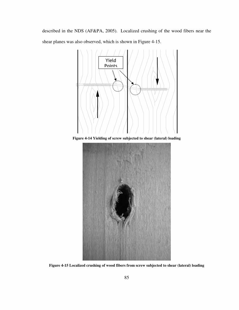
85
described in the NDS (AF&PA, 2005). Localized crushing of the wood fibers near the
shear planes was also observed, which is shown in Figure 4-15.
Figure 4-14 Yielding of screw subjected to shear (lateral) loading
Figure 4-15 Localized crushing of wood fibers from screw subjected to shear (lateral) loading
Yield Points

86
4.6 Moisture Content and Specific Gravity
Moisture content and oven dried specific gravity tests were conducted on each
piece of timber used in the physical testing. Moisture content and specific gravity tests
were also conducted for each pair of oak wedges. Moisture content tests were conducted
according to the secondary oven drying method included in ASTM D4442, and specific
gravity tests were conducted according to ASTM D2395 (ASTM, 2007).
Samples were cut from the test specimens within several hours after testing. The
samples were taken from a representative section of the material away from any exposed
end-grain. The dimensions of each sample were measured to the nearest 0.001” using
calipers in two locations in each direction. The initial weight was recorded to the nearest
0.01g using a digital scale. Samples were then placed in a vented lab oven set to 217ºF.
Samples were removed from the oven after their weight had stabilized or after 48 hours,
whichever was longer. Results for the moisture content and specific gravity tests are
included with the individual test data.
4.6.1 Adjustments in Modulus of Elasticity Based on Moisture Content
The moisture content of solid sawn material can vary greatly between the time the
wood is harvested and when it is finally put into service. Changes in relative humidity
can also affect the moisture content of wood in service. Wood’s mechanical properties
are sensitive to the moisture content of the material. Common wood science procedure is
to use mechanical properties at 12% moisture content. Therefore during the small and

87
full scale testing, test results were adjusted to 12% moisture content when the material
tested was wetter or drier than 12%.
The relationship between moisture content and material properties is described
according to the Wood Handbook (FPL, 1999) as
12
12
12%12%
MC
MP
green
EE E
E
−
− =
(4-2)
where MC is the moisture content in percent and MP is a species-specific constant that
is slightly less than the fiber saturation point. Unless otherwise known, 25MP = for
most hardwood species. The 12%
E and green
E values are taken from Table 4-3b of the
Wood Handbook. When the moisture content exceeded 25%, which is the fiber
saturation point of most hardwoods, the values for green material were used.
4.6.2 Adjustments in Modulus of Elasticity Based on Specific Gravity
The mechanical properties of wood are directly and positively correlated to its
density. Thus, woods with higher specific gravities tend to have higher strengths and
stiffnesses than those with lower specific gravities. To account for this, the Wood
Handbook (FPL, 1999) lists a the relationship for all hardwood species at 12% moisture
content as
0.72,390,000E G psi= (4-3)
which pertains to usage with the white oak material. The Wood Handbook also lists the
relationship for all softwood species at 12% MC as
0.842,970,000E G psi= (4-4)

88
While yellow poplar is technically a hardwood, it behaves in certain fashions more like a
softwood. A graphical comparison of equations (4-3) and (4-4) with the modulus of
elasticities determined from the small scale bending tests suggest equation (4-4) is most
appropriate for yellow poplar (Figure 4-16).
1250000
1300000
1350000
1400000
1450000
1500000
1550000
1600000
1650000
1700000
0.350 0.370 0.390 0.410 0.430 0.450 0.470 0.490
Specific Gravity
Mo
du
lus o
f E
lasti
cit
y (
psi)
Unadjusted MOE
Hardwood MOE Eqn
Softwood MOE Eqn
Figure 4-16 Comparison of Wood Handbook MOE equations to test data (typical)
To adjust the tabulated modulus of elasticity from the Wood Handbook for a
particular test, the relationships shown in equations (4-3) and (4-4) were used to calculate
an appropriate scaling factor and thus an adjusted modulus of elasticity. For white oak,
the adjusted modulus of elasticity is calculated as
0.70239
1,780,000178
ADJUSTED
GE psi
=
(4-5)
where 1,780,000 psi is the Wood Handbook published modulus of elasticity for white oak
at 12% moisture content. For yellow poplar, the adjusted modulus of elasticity is
calculated as

89
0.84297
1,580,000158
ADJUSTED
GE psi
=
(4-6)
where 1,580,000 is the Wood Handbook published modulus of elasticity for yellow
poplar at 12% moisture content.

90
5 Full Scale Beam Testing
In order to verify the adequacy of the interlayer slip model for modeling the actual
behavior of keyed beams, full scale keyed beam testing was conducted. This full scale
testing consisted of loading four keyed beams; two with white oak keys, two with
Parallam PSL keys. Two additional tests were conducted on a full-sawn beam and a
simple stacked beam (no interaction between layers) to verify the upper and lower
bounds on stiffness. The loading configuration for all of the beam tests is shown in
Figure 3-7, with the keyed beam layout is shown in Figure 3-6.
5.1 Beam Fabrication
All beams were delivered to the testing lab in the unplaned, green (unseasoned)
moisture condition sawn to the full dimension. Due to an extended period of time
between the delivery of the material and the testing, significant drying, shrinkage, and
checking occurred in the timbers. However, any preparation and fabrication of the
stacked beams and keyed beams used in the full-scale testing was completed no more
than 24 hours before the time of testing.
No preparation was required for the full-sized 8 inch by 16 inch beam, other than
ensuring the bearing points were flat and orthogonal to the applied load and support
reactions. Flat bearing points were also created on the two 8 inch by 8 inch stacked
beams. The contact faces between the two stacked beams were planed with an electric
hand planer to ensure uniform contact between layers.

91
Keyed beams were fabricated by first mating pairs of 8 inch by 8 inch timbers that
had similar amounts of crown. Timbers were also oriented such that any seasoning
check (or most substantial seasoning check if checked on multiple faces) was on a
horizontal face (top or bottom). Although most timbers were relatively free of knots,
timbers that exhibited the most knots were used as the top (compression) layer. The
mating faces between the two timbers were then planed to ensure uniform contact
between layers. The two layers where temporarily secured together when marking key
notch locations on the timbers. This temporary clamping ensured all notches were
aligned properly along the entire length of the timbers. Notches were cut using a circular
saw and cleaned up using a framing chisel. All exposed end-grain was sealed with end-
grain sealer after cutting.
Keyed beam layers, once notched (Figure 5-1(a)), were secured together with the
LogHog screws about the entire length before any shear keys were installed. Before the
screws were installed, the timbers were clamped together, which can be seen in Figure
5-1(b), to ensure uniform contact between layers. The clamping of the timbers together
before insertion of the screws follows common timber construction practices. The
locations for the LogHog screws can be found in Figure 3-6. Once the layers were fully
secured together, the shear key wedges were installed. The shear key wedges were
tightened by pounding on opposing wedges immediately before the testing commenced.
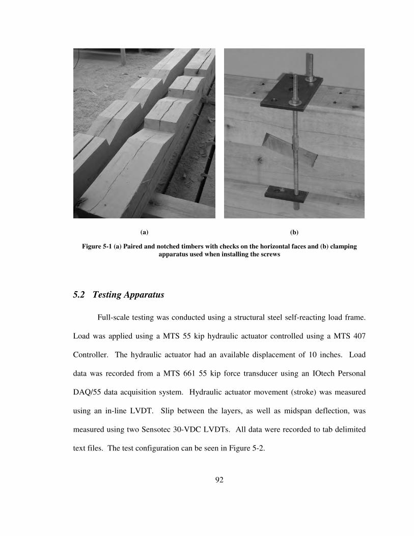
92
(a)
(b)
Figure 5-1 (a) Paired and notched timbers with checks on the horizontal faces and (b) clamping
apparatus used when installing the screws
5.2 Testing Apparatus
Full-scale testing was conducted using a structural steel self-reacting load frame.
Load was applied using a MTS 55 kip hydraulic actuator controlled using a MTS 407
Controller. The hydraulic actuator had an available displacement of 10 inches. Load
data was recorded from a MTS 661 55 kip force transducer using an IOtech Personal
DAQ/55 data acquisition system. Hydraulic actuator movement (stroke) was measured
using an in-line LVDT. Slip between the layers, as well as midspan deflection, was
measured using two Sensotec 30-VDC LVDTs. All data were recorded to tab delimited
text files. The test configuration can be seen in Figure 5-2.

93
Figure 5-2 Full scale beam test configuration

94
5.3 Test Results
5.3.1 Full and Stacked Beams
The full depth and simple stacked beams were loaded until approximately 25% of
the anticipated modulus of rupture was reached. The beams were then unloaded and cut
into smaller pieces for use with the small scale testing discussed in section 4. The full
depth beam displayed ring-shake at one end coupled with a substantial seasoning check
(Figure 5-3). The simple stacked beams were relatively clear and defect free. During
testing of the simple stacked beam, audible “clicking” was heard, which was attributed to
the slipping between the layers. This phenomenon was also audible during the white oak
key testing (section 4.4.1).
The load-deflection plots indicated slight initial softness, followed by very linear
behavior until the test was stopped. The load-deflection plots, along with those for the
keyed beam tests, can be found in Figure 5-4. As anticipated, the full depth beam
provides an upper bound on stiffness for all of the beam tests, whereas the simple stacked
beam acts as a lower bound. The stiffness of each keyed beam tests falls between the full
depth and simple stacked beam stiffnesses. Moisture content, specific gravity, and
stiffness data is included in Table 5-1.

95
Figure 5-3 Ring-shake and checking in the full depth beam
Longitudinal displacement between the layers (slippage) was recorded at both
ends of the simple stacked span using LVDTs. The slippage at the ends was 0.139 inch
and 0.073 inch (0.106 inch average) at 10 kips of applied load, compared to an
anticipated 0.118 inch. Appendix G includes the procedure for determining the
anticipated slip. A similar measurement was taken during the full depth test at the
beam’s neutral axis, although no movement was observed, as expected.

96
0
5
10
15
20
25
30
35
40
45
0 0.5 1 1.5 2 2.5 3
Deflection at point loads (in)
To
tal
Lo
ad
(kip
s)
Full Depth & Stacked
White Oak Keys
Parallam PSL Keys
Figure 5-4 Load-deflection plots of full-scale beam tests
Table 5-1 Full-scale beam test results
Test b (avg) d (avg)
Moisture
Content
(avg)
Specific
Gravity
(avg) Material
Moisture
Content
(avg)
Specific
Gravity
(avg)
Actual I
(Full
Depth) Stiffness
Apparent
E
in in in^4 lb / in psi
Full 7.59 15.53 21.2% 0.443 2371 38400 1254000
Stacked 7.69 7.63 15.6% 0.429 2277 11200 381000
1 7.61 7.06 16.0% 0.453 WO 33.4% 0.638 1785 15100 655000
2 7.72 7.44 11.4% 0.407 WO 26.5% 0.632 2120 17300 632000
3 7.58 7.50 10.3% 0.367 PSL 7.8% 0.605 2132 24500 889000
4 7.59 7.45 11.8% 0.424 PSL 7.9% 0.607 2092 28000 1036000
Timber Key
In Table 5-1 above, the “Actual I” represents the moment of inertia for the full
beam cross-section. “Apparent E” is the apparent modulus of elasticity (modulus of
elasticity including shear deformations) of a partially-composite beam based on a full
depth beam cross sectional properties.

97
5.3.2 Keyed Beams with White Oak Shear Keys
Two keyed beams with white oak shear keys and identical configurations were
tested on the same load frame and in the same manner as the full depth and simple
stacked beams. Load-deflection plots are shown in Figure 5-4 and pertinent test data is
tabulated in Table 5-1. The deflection shown in Figure 5-4 is recorded as the movement
of the hydraulic actuator. Load was applied until failure occurred.
For the first beam, failure occurred at 34.1 kips of applied load, and occurred
when cracking in the bottom face of the bottom layer appeared, which coincided with a
slight drop in load. While the beam appeared to be able to still resist some loading, the
test was inadvertently interrupted, so no additional load was applied. The keyed beam is
shown in Figure 5-5. Audible “ticking” was again apparent during the testing.
Horizontal slip was measured using LVDTs mounted at each end of the beam, and a load-
slip plot is shown in Figure 5-6. The shape of the load-slip plots suggests similar
behavior, as anticipated, at each end of the beam. The non-linear shape of the plots,
when compared to the linear behavior of the full depth and simple stacked beams,
suggests slippage did not occur at a uniform rate, which is related to the non-linear
behavior of the beam load-deflection plots shown in Figure 5-4. After testing, the shear
keys were removed from the keyed beam, and the shear keys near the ends of the beam
exhibited substantial deformation, similar to those from the small-scale key tests (Figure
4-12). The shear keys near the center of the span exhibited substantially less
deformation. This uneven load distribution between keys is most likely the culprit for the
non-linear behavior seen in the load-deflection and load-slip plots (Figure 5-4,Figure

98
5-6), as keys nearer the beam end reached their crushing point sooner than those near the
middle.
Figure 5-5 Keyed beam using white oak shear keys under load

99
0
5
10
15
20
25
30
35
0 0.05 0.1 0.15 0.2 0.25 0.3 0.35 0.4
Slip (in)
To
tal
Lo
ad
(kip
s)
Test 1
Test 2
Figure 5-6 Load-slip plots for white oak shear key tests
For the second beam, failure consisted of a sudden tensile failure of the bottom
layer which propagated nearly instantly upwards to the center of the top layer. This
sudden breakage occurred at an applied load of 39.6 kips, and the beam failed to carry
any additional load after breaking. The broken keyed beam, which is shown in Figure
5-7, exhibits similar cracking behavior to that seen in the small scale flexure tests (Figure
4-2). Once the beam failed, additional cracks propagated from the re-entrant corners of
the inner shear keys (Figure 5-8). These cracks were not apparent before sudden failure
of the beam. Slip between the layers was only measured at one end of the beam for this
test, as the results from test 1 showed very similar movements at each end. The other
LVDT was placed under the midspan of the beam to confirm vertical displacement under
loading, and quantify the compliance in the test frame and supports (see section 5.4.3).
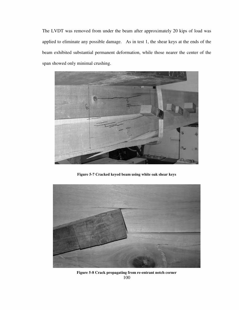
100
The LVDT was removed from under the beam after approximately 20 kips of load was
applied to eliminate any possible damage. As in test 1, the shear keys at the ends of the
beam exhibited substantial permanent deformation, while those nearer the center of the
span showed only minimal crushing.
Figure 5-7 Cracked keyed beam using white oak shear keys
Figure 5-8 Crack propagating from re-entrant notch corner

101
5.3.3 Keyed Beams with Parallam PSL Shear Keys
Two keyed beams of identical configuration were tested using Parallam PSL
shear keys. These beams had the same layout as the keyed beams with white oak shear
keys discussed in the previous section. Mid-span deflection was measured along with
interlayer slip at one end of the beams. Load-deflection plots for these tests can be found
in Figure 5-4, which show very linear behavior up until the point of buckling. Despite
efforts to brace the hydraulic loading ram, the beam buckled laterally due to three-hinged
column action, with two hinges (points of rotation) occurring at the top and bottom pins
on the hydraulic ram, and the third hinge (point of rotation) occurring where the beam sat
atop the test-frame supports. Other pertinent test data is included in Table 5-1. Figure
5-9 shows a loaded beam shortly before buckling occurred.
The first Parallam PSL-keyed beam buckled suddenly at a load of 42.4 kips. For
the next test, additional bracing was added to the hydraulic ram and considerable effort
was taken to ensure the ram and beam were plumb and square. Despite these efforts, the
second beam still buckled at a lower load level than the first (35.1 kips). The ultimate
loads for both keyed beams using Parallam PSL keys was controlled by the loading
instability, not material failure.
Timber beams with a depth-to-breadth ratio of 2:1 or less do not normally fail in
lateral torsional buckling, and bracing is not required for their in-service use (AF&PA,
2005). The keyed beams tested in this research have a depth-to-breadth ratio of 2:1, so
lateral bracing of the beam was not initially included. To limit the possibility of
damaging equipment or risking injury, no additional testing was conducted on the

102
Parallam PSL-keyed beams after they buckled. Therefore, ultimate load of the Parallam
PSL-keyed beams was never reached.
Unlike the white oak-keyed beams, the Parallam PSL-keyed beams had the
prevalent audible “ticking” noise from interlayer slipping only until around 10 kips of
load. After 10 kips of load, the frequency of ticks diminished, and the ones that occurred
were considerably less audible. Slight cracking noises were heard in the beams shortly
before buckling occurred as well. The cracking may have been from fibers nearing their
rupture point, but was more likely an indication of the impending buckling. Very little
slip was noticed between the layers during testing, and the keys did not appear to rotate
or compress. After the testing, the keys were removed from the beam, and no end-grain
crushing of the keys or the timbers was apparent. However, crushing of the keys or end-
grain may have occurred if the beams had reached the material failure capacity before
reaching the buckling/stability capacity of the load frame.

103
Figure 5-9 Parallam PSL-keyed beam under load
5.4 Adjustments to Test Results
As with the small scale testing, the moisture content, specific gravity, and cross
sectional dimensions varied between each timber used in the full-scale beam testing. The
moisture content and specific gravity also varied in the white oak shear keys. In order to
compare the results between the different tests, adjustments to the keyed beam test

104
stiffnesses were made to account for these variations. These adjustments are based on
published relationships between modulus of elasticity and specific gravity and moisture
content (FPL, 1999).
5.4.1 Moisture Content and Specific Gravity
The stiffnesses of the keyed beam tests were adjusted for variations in moisture
content and specific gravity of the timbers. The process used is similar to that set forth in
section 4.6 for the small scale testing. With the assumption that modulus of elasticity of
the timbers a controlling factor in beam and following section 4.6.1, the adjustment for
moisture content (FPL, 1999) is
12%
12
1312% 12%
green
ADJ UNADJ MC
green green
E
EK K
E E
E E
−
=
(5-1)
where UNADJ
K is the unadjusted stiffness of a particular test, 12%
E is the published modulus
of elasticity for yellow poplar at 12% moisture content (1,580,000psi), green
E is the
published green moisture content (1,220,000psi), and MC is the averaged moisture
content of the timbers at the time of testing. Equation 5-1 simplifies to
12
13158
122
MC
ADJK
−
=
(5-2)
In a similar fashion to the procedure outlined in 4.6.2, it is possible to adjust the
keyed beam test stiffness for variations in specific gravity (FPL, 1999) by

105
0.84 0.84
12% 12%
0.84 0.84
2.97
2.97ADJ UNADJ UNADJ
ACT ACT
G GK K K
G G= = (5-3)
where 12%
G is the published specific gravity for yellow poplar (0.42) and ACT
G is the
actual specific gravity of the beam at the time of testing determined using ASTM D2395
(ASTM, 2007). The adjusted stiffness values for the full-scale beam tests, which include
all of the applicable adjustments, are shown in Table 5-2. Although only two tests of
each type were conducted, a comparison of the values for the white oak keyed beams and
for the Parallam PSL keyed beam shows these adjustments reduced a substantial amount
of variation in the actual beam stiffnesses. In Table 5-2, “Apparent E” is the modulus of
elasticity of a partially-composite beam based on a full depth beam cross sectional
properties.
Table 5-2 Adjusted stiffness values for full-scale beam tests
Test Actual I Stiffness
Stiffness
(adjusted)
Apparent
E
Apparent
E
(adjusted) Efficiency
in^4 lb / in lb / in psi psi
Full 2371 38400 39200 1254000 1281000 100.0%
Stacked 2277 11200 10900 381000 372000 29.0%
1 1785 15100 18100 655000 787000 61.4%
2 2120 17300 17500 632000 639000 49.9%
3 2132 24500 26300 889000 954000 74.5%
4 2092 28000 27900 1036000 1032000 80.6%
The moisture content and specific gravity data of the white oak shear keys used in
the first two keyed beam tests was not used to adjust the stiffness of the keyed beam tests
in this section (i.e., the “Apparent E” has not been adjusted to account for variations in
key specific gravity and moisture content). This white oak key specific gravity and
moisture content data is included in section 6 when comparing the keyed beam tests to
the anticipated results from the interlayer slip model outlined in section 2.

106
5.4.2 Variations in Cross Section
Slight variations in cross-section can greatly impact the stiffness of both simple
beams as well as keyed beams, with the moment of inertial being the cross-sectional
property controlling flexural stiffness behavior. To account for these variations so all of
the tests can be compared on consistent basis, the stiffness of each test was adjusted to a
7.5 inch wide by 15 inch deep timber by
( )( )
3
3
(7.5)(15)
12 2109.375
12
ADJ UNADJ UNADJ
ACTUALact act
K K KIb d
= =
(5-4)
where act
b and act
d are the actual beam breadth and depth in inches. These adjustments
to account for variations in cross section have been applied to the adjusted stiffness
values in Table 5-2.
5.4.3 Test Frame Compliance
During all of the tests, beam deflection was measured using the stroke movement
of the hydraulic ram. This measurement of deflection may include flexural deflection,
crushing of bearing plates, and other test frame compliance issues. In order to isolate the
effects of frame compliance, additional deflection measurements were taken during the
testing of the second white oak keyed beam, along with both of the Parallam PSL keyed
beams, using an LVDT. The LVDT was placed under the beam near midspan, and
recorded movement of the bottom edge of the beam compared to the base of the test
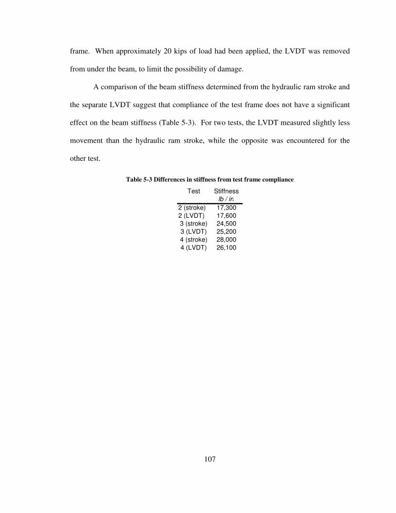
107
frame. When approximately 20 kips of load had been applied, the LVDT was removed
from under the beam, to limit the possibility of damage.
A comparison of the beam stiffness determined from the hydraulic ram stroke and
the separate LVDT suggest that compliance of the test frame does not have a significant
effect on the beam stiffness (Table 5-3). For two tests, the LVDT measured slightly less
movement than the hydraulic ram stroke, while the opposite was encountered for the
other test.
Table 5-3 Differences in stiffness from test frame compliance
Test Stiffness
lb / in
2 (stroke) 17,300
2 (LVDT) 17,600
3 (stroke) 24,500
3 (LVDT) 25,200
4 (stroke) 28,000
4 (LVDT) 26,100

108
6 Analysis of the Interlayer Slip Model using Full Scale Test Data
An accurate analytical interlayer slip model is desirable, as it would permit a
reasonable design procedure. Therefore, comparing the anticipated behavior of a keyed
beam from the interlayer slip model with full-scale physical test data becomes a primary
focus in this research.
6.1 Comparison of Test Data
In order to compare physical test data from previous sections, data was adjusted to
a normalized value to account for variations in moisture content, specific gravity, and
cross sectional dimensions of the timbers. These adjustments were required to permit a
direct comparison of the results from different test configurations. In this section, the
focus is on comparing results from full-scale beam tests to predicted results from the
interlayer slip model. The interlayer slip model can directly account for variations in
section properties and elastic moduli. Therefore, material and section properties from the
in situ test conditions will be used, rather than normalized values.
6.1.1 Interlayer Slip Model Input Parameters
In order to use the interlayer slip model developed in section 2, several material
and section properties are required. Before the cross sectional areas and moment of
inertias can be calculated, the breadth b and depth d of the individual timbers are
required. To determine the timber’s modulus of elasticity, the moisture content MC and
specific gravity G are also required. For the shear keys, the key thickness t is required
to determine the key stiffness. Also, for the white oak keys, the shear key moisture

109
content and specific gravity is also required to determine the modulus of elasticity. For
the Parallam PSL keys, the manufacturer’s published values for modulus of elasticity
were used. The various section properties can be found in Table 6-1.
Table 6-1 Physical data on keyed beam tests for use with the interlayer slip model
Test Layer b d A MC G Etim (calc)
in in in2
% psi
top 7.63 7.49 57.1 17.4% 0.465 1547000
btm 7.59 6.63 50.3 14.7% 0.441 1561000
top 7.69 7.38 56.8 10.4% 0.361 1391000
btm 7.75 7.50 58.1 12.4% 0.452 1666000
top 7.56 7.44 56.2 9.3% 0.327 1280000
btm 7.60 7.56 57.5 11.4% 0.406 1536000
top 7.57 7.39 55.9 12.9% 0.442 1620000
btm 7.61 7.50 57.1 10.7% 0.405 1532000
Avg 12.4% 0.412 1517000
Test Key t MC G Ekey (calc)
in % psi
A 2.51 37.2% 0.678 1247000
B 2.47 32.9% 0.628 1180000
C 2.44 30.1% 0.608 1153000
A 2.48 22.0% 0.652 1213000
B 2.38 29.0% 0.630 1184000
C 2.50 28.4% 0.614 1161000
A 2.41 7.8% 0.605 2100000
B 2.44 7.8% 0.605 2100000
C 2.42 7.9% 0.606 2100000
A 2.44 7.9% 0.606 2100000
B 2.41 8.0% 0.608 2100000
C 2.43 7.9% 0.607 2100000
1
2
3
4
3
4
1
2

110
Actual modulus of elasticity values for individual timbers and shear keys were not
able to be directly measured. In order to calculate these values, the published
relationships between modulus of elasticity and moisture content and specific gravity
were used (FPL, 1999).
For the timbers, the relationship between specific gravity and modulus elasticity
for softwoods was used for material at 12% moisture content (see section 4.6.2). The
actual timber modulus of elasticity tim
E in psi was calculated as
0.84
0.84
0.421,580,000
tim
tim
EG
=
(6-1)
where 1,580,000 is the modulus of elasticity for yellow poplar at 12% moisture content,
0.42 is the published specific gravity of yellow poplar at 12% moisture content, and tim
G
is the oven dry specific gravity of the timber based on volume at approximately 12%
moisture content (FPL, 1999). Note this modulus of elasticity is predicting the actual
modulus of elasticity of the timber at the time of testing; it is not a modulus of elasticity
normalized to a particular moisture content or specific gravity, as discussed in previous
sections. These calculated modulus of elasticies are found in Table 6-1.
The modulus of elasticity for the white oak shear keys was calculated using the
published relationship between it and specific gravity for green hardwood material (FPL,
1999). The shear key modulus of elasticity key
E in psi was determined by the
relationship
0.72
0.72
0.681,250,000
key
key
EG
=
(6-2)

111
where 1,250,000-psi is the modulus of elasticity for green white oak, 0.68 is the specific
gravity of white oak at 12% moisture content, and key
G is the oven dry specific gravity of
the shear key based on green volume (FPL, 1999). These calculated elastic moduli are
included in Table 6-1. Keys designated by “A” are the keys that were closest to the ends,
where as the “C” keys were those closest to the center of the beam and applied point load.
To provide symmetry during physical testing, the shear keys closest to the ends of the
beams were cut from the same piece of material. Likewise the shear keys closest to the
point loads were cut from the same piece of material, and the middle set of shear keys
were also fabricated in a similar fashion.
Adjustments to timber and key modulus of elasticity due to variations in moisture
content were made in a fashion similar to that shown in equation 5-2 (see section 5.4.1),
such that
12
13
12%12%
MC
calc
green
EE E
E
−
=
(6-3)
where 12%
E and green
E are the published modulus of elasticity values for a given species,
taken from the Wood Handbook (FPL, 1999), and MC is the moisture content, in
percentage, of the material. Most of the white oak shear keys exceeded the average fiber
saturation point for most hardwoods of 25% (FPL, 1999). Mechanical properties, in
particular modulus of elasticity, do not vary significantly with changes in moisture
content above the fiber saturation point. When a material’s moisture content was above
the fiber saturation point, 25% was used instead.

112
6.1.2 Analysis Results
The solution of the interlayer slip model equations for a two-layer beam with
symmetrically placed point loads was used for this comparison. The development of the
solution is included in Appendix C. The analysis and specific solutions of the interlayer
slip model based on the full-scale test data parameters are included in Appendix H. The
results of the analyses can be seen in Table 6-2. A graphical comparison of the load-
deflection plots from testing and the analytical solution using the interlayer slip model are
shown in Figure 6-1.
Table 6-2 Comparison of analytical and full-scale testing stiffnesses
Test Key Model Test Difference
lb/in lb/in %
1 OAK 16806 15100 10.2%
2 OAK 19228 17300 10.0%
3 PSL 26558 24500 7.7%
4 PSL 28708 28000 2.5%
Avg. 7.6%

113
0
5
10
15
20
25
30
35
40
45
0 0.5 1 1.5 2 2.5 3
Deflection (in)
To
tal
Lo
ad
(kip
s)
White Oak Keys
Parallam PSL Keys
Model (OAK)
Model (PSL)
Full Depth
Stacked
Figure 6-1 Comparison of load-deflection plots and interlayer slip model solutions
The stiffnesses from the interlayer slip model were slightly higher than the actual
test results in all four comparisons, although by an average value of only 7.6%. For
flexural members, whether simple stacked, full depth, or composite beams, the modulus
of elasticity of the material has a dominant effect on the stiffness of the member. The
published average coefficient of variation for timber modulus of elasticity is 0.22 (FPL,
1999), suggesting that variations between the calculated and actual keyed beam
stiffnesses may be attributed to natural variations in modulus of elasticity of the material.
The slightly larger difference between the calculated and actual stiffnesses for the
keyed beams using white oak keys may be attributed to the non-linear behavior of these

114
tests. As was discussed in 5.3.2, the physical testing showed a disparate amount of shear
key crushing between the shear keys nearest the beam ends and those closest to midspan,
which is likely due to non-linear behavior and beam softening. Also, the non-linear
shape of the load-deflection plots means some subjectivity is required when determining
the initial stiffness from the straight-line portion.
The small-scale white oak shear key tests discussed in section 4.4 exhibited a bi-
linear behavior (Figure 4-9); an initial stiff region followed by secondary region of
substantially less stiffness. This bi-linear behavior is quite common in wood when it is
subjected to cross-grain compressive forces (ASTM D143, 2007). The development of a
bi-linear model for the cross-grain stiffness of the white oak shear keys would better
capture the actual behavior of the shear keys. Using this bi-linear stiffness in the
interlayer slip model would more accurately capture the non-linear behavior exhibited in
testing. However, the small difference (7.6%) between the stiffnesses from the physical
testing and the interlayer slip model do not appear to justify the additional computational
effort required to perform a non-linear analysis.
6.2 Shear Key Spacing Methodology
The interlayer slip model requires calculating two constants, F
C and M
C , which
can be found in equations (2-18) and (2-19). Both of these constants include a
component for determining the stiffness per unit length of the shear keys, i
i
K
s∑ . The
individual key stiffness K is calculated by the process developed in section 2.5, but
determining the appropriate key spacing distance s each shear key acts over is less

115
certain. This section investigates several possible approaches to calculating an
appropriate key spacing, and compares the various outcomes when each approach is used
in conjunction with the interlayer slip model.
6.2.1 Simplified Approach
Perhaps the simplest approach for determining the effective stiffness per unit
length is to sum all of the shear key stiffnesses and distribute this evenly over the entire
length of the beam, such that
i
K
L
∑ (6-4)
This approach, which was used to calculate the beam stiffnesses in section 6.1, is based
on the assumption that there is even load distribution between each shear key. The full-
scale beam tests conducted with white oak shear keys showed substantially different
amounts of crushing in the shear keys, suggesting that even load distribution is perhaps
not appropriate. The PSL-keyed beams did not display disparate deformation between
individual shear keys, suggesting they may have carried load evenly. However, the
material failure load of these beams was never reached. This simplified approach for
determining effective stiffness more accurately predicts the stiffness of the beams with
the Parallam PSL keys than the beams with white oak keys.
6.2.2 Shear Stud / Composite Beam Approach
Steel-concrete composite beams are commonly found in commercial construction.
A wide-flange steel section is on the bottom (tension portion) of the composite beam, and
a cast-in-place concrete deck is used on the top (compression portion). The initial

116
interlayer slip model, developed by Newmark, was intended to model this specific type of
beam (Newmark, 1951). The approach used when determining the number of shear studs
for these types of composite beams includes making a section cut at any point along the
beam, and the shear studs in that section must be able to resist the difference in the
tension and compression force components generated by composite action. Common
design procedure for steel-concrete composite beams used as bridge girders is to have
varying shear stud spacing, to account for the varying shear about the length from a
uniformly distributed load, whereas a uniform shear key spacing is more common for
steel-composite beams used in occupied structures. For the keyed beam configuration
used in this testing, the moment in the beam (Figure 3-7) varies linearly between the
reaction and applied point loads resulting in a constant shear and key spacing.
In order to use this composite beam approach with this keyed beam testing, it was
assumed each shear key resisted the forces starting at the shear key heel except for the
end key. The resultant spacing and points of assumed action are shown in Figure 6-2.
s =34" s =18" s =32.5"
81.5"
1 2 3
Figure 6-2 Assumed shear key spacing using a composite beam approach

117
The lowest stiffness term ( i
i
K
s) is associated with the shear key nearest the end of
the beam, while the highest stiffness term is associated with the middle key. Using a
springs in parallel analogy, the majority of the force being resisted should be carried by
the stiffest “spring”, which corresponds with the middle key. However, the assumed
spacing shown in Figure 6-2 does not appear consistent with the observed key crushing
from the white oak tests. Results from the interlayer slip model (included in Table 6-3)
using these shear key spacings predict substantially stiffer keyed beams than were
observed.
Table 6-3 Comparison of various methods for determining shear key spacing
Test Method Difference
Calculated Actual %
Simple 16806 10.2%
Composite 23994 37.1%
Trib. Width 24060 37.2%
Simple 19228 10.0%
Composite 27514 37.1%
Trib. Width 27582 37.3%
Simple 26558 7.7%
Composite 33138 26.1%
Trib. Width 33172 26.1%
Simple 28708 2.5%
Composite 36198 22.6%
Trib. Width 36234 22.7%
7.6%
Avg. 30.7%
30.8%
1
2
3
4
17300
24500
28000
Beam Stiffness (lb/in)
15100
6.2.3 Tributary Length Approach
In structural analysis, a common design approach for determining load paths is
using a tributary area approach, where forces or loads are distributed based on half the

118
distance between points of interest. Using this approach, the corresponding spacings
between keys were determined (Figure 6-3).
s =29.2"
81.5"
s =18" s =37.3"1 2 3
Figure 6-3 Assumed shear key spacing using tributary length approach
Like the composite beam approach, the highest stiffness term ( i
i
K
s) is associated
with the middle shear key. However, the lowest stiffness term using the tributary length
approach is in the shear key nearest the center of the span. This appears to match the
observed crushing behavior of the white oak shear keys better than the composite beam
approach. However, this method results in the same predicted stiffness of the keyed
beams as the composite beam approach, which is considerably stiffer than the observed
beam behavior (Table 6-3).
6.2.4 Recommended Spacing Calculation
The composite beam and tributary length approaches are quite common in design,
although appear to capture beam behavior worse than a simplified approach. Based on
the shear flow diagrams (see Figure 2-12a and Figure 2-12b), the variations in the full
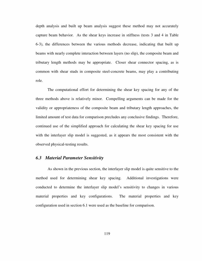
119
depth analysis and built up beam analysis suggest these method may not accurately
capture beam behavior. As the shear keys increase in stiffness (tests 3 and 4 in Table
6-3), the differences between the various methods decrease, indicating that built up
beams with nearly complete interaction between layers (no slip), the composite beam and
tributary length methods may be appropriate. Closer shear connector spacing, as is
common with shear studs in composite steel-concrete beams, may play a contributing
role.
The computational effort for determining the shear key spacing for any of the
three methods above is relatively minor. Compelling arguments can be made for the
validity or appropriateness of the composite beam and tributary length approaches, the
limited amount of test data for comparison precludes any conclusive findings. Therefore,
continued use of the simplified approach for calculating the shear key spacing for use
with the interlayer slip model is suggested, as it appears the most consistent with the
observed physical-testing results.
6.3 Material Parameter Sensitivity
As shown in the previous section, the interlayer slip model is quite sensitive to the
method used for determining shear key spacing. Additional investigations were
conducted to determine the interlayer slip model’s sensitivity to changes in various
material properties and key configurations. The material properties and key
configuration used in section 6.1 were used as the baseline for comparison.

120
6.3.1 Modulus of Elasticity of Timbers
For both full depth beams and simple stacked beams, the timber modulus of
elasticity is the only material property that affects the flexural stiffnesses. Thus, using the
interlayer slip model to determine the stiffness of keyed beams should also be sensitive to
changes in the timber modulus.
The published average modulus of elasticity from the Wood Handbook (FPL,
1999), adjusted for specific gravity, was used in this research. In order to examine the
interlayer slip model’s sensitivity to variations in timber modulus, the four analyses
conducted in section 6.1 were reexamined using timber modulus one standard deviation
higher and lower than the published average. The coefficient of variation for modulus of
elasticity of small, clear wood specimens is 0.22 (FPL, 1999). For a yellow poplar timber
at 12% moisture content, the average published specific gravity is 1,580,000 psi (FPL,
1999) which results in a lower bound for the sensitivity analysis of 1,232,000 psi and an
upper bound of 1,928,000 psi. No adjustments were made to these values for variations
in specific gravity.
As anticipated, the interlayer slip model stiffness was very sensitive to changes in
timber modulus of elasticity (Table 6-4). Changes in timber modulus result in a nearly
linear response in beam stiffness across the evaluated range. Based on these
observations, knowing the timber modulus of elasticity is unsurprisingly crucial in
predicting the beam stiffness. This observation holds true whether the beam is a solid
beam or one with partial interaction between layers.

121
Table 6-4 Variations in stiffness with changes in timber modulus of elasticity
-1 Std Dev Avg +1 Std Dev
Test lb/in lb/in lb/in
1 14246 17012 19600
2 16488 19682 22674
3 23760 29332 34556
4 23312 28782 33910
Beam Stiffness
6.3.2 Cross-grain Modulus of Elasticity
The shear keys are the link between the individual layers of a built-up beam, so
variations in their modulus (and thus stiffness) are anticipated to have a direct correlation
to the amount of interaction that occurs between the beam layers. Therefore, the
sensitivity of the interlayer slip model to changes in the shear key modulus of elasticity
was also investigated.
Published data for most wood species includes the longitudinal modulus of
elasticity. If the shear keys are installed such that they are being loaded parallel to the
grain, this published value can be used directly. However, with solid wood keys,
installing wedge shear keys in such a fashion proved problematic (see section 3.2.2), so
solid wood keys were installed such that they were being compressed across the grain.
Compressing the keys across the grain requires the use of elastic ratios, as species
specific published cross-grain modulus values are not readily available.
The elastic ratio assumed earlier for analysis purposes was 12E E⊥=�
for both the
timber and key material. For this sensitivity study, several other ratios were examined
(1:1, 1:2, 1:4, 1:8, 1:16, 1:20, 1:24), with the timber and key material always maintaining
the same ratio. The analysis process was similar to that conducted in section 6.1, with no

122
changes to the other material properties. The results of these analyses are plotted in
Figure 6-4.
14000
16000
18000
20000
22000
24000
26000
28000
30000
32000
0 0.1 0.2 0.3 0.4 0.5 0.6 0.7 0.8 0.9 1
Eperp / Epar
Sti
ffn
ess (
lb/i
n)
1
2
3
4
Figure 6-4 Relationship between elastic ratio and calculated beam stiffness for each beam test
For beam tests 1 and 2, the white oak keys were installed such that they were
being compressed perpendicular to their grain, and thus the interlayer slip model was
quite sensitive to changes in the assumed elastic ratio. With beam tests 3 and 4, Parallam
PSL was used for the shear keys, which were being compressed parallel to the grain.
Thusly, the variation of the elastic ratios did not affect the stiffness of the key, only the
angle to the grain bearing stiffness of the timber at the face of the key. As the elastic
ratio approached 1:1, the key stiffness had less effect on the overall stiffness of the beam.

123
The stiffness data from the interlayer slip model analyses using various elastic
ratios was compared to the observed stiffness from the full-scale beam testing. The
average difference between the observed and modeled stiffness are shown in Figure 6-5.
An elastic ratio of 19.2E E⊥=�
(0.052E E⊥=�
) results in no average difference between
the observed and modeled keyed beam stiffnesses. This ratio compares closely to an
elastic ratio of 1:20 suggested by Bodig and Jayne (1982). Although using an elastic
ratio of 1:20 appears to be more appropriate than the originally assumed ratio of 1:12, the
small-scale key testing showed an optimal elastic ratio of 1:12.7 (section 4.4.3). The
limited number of small-scale and full-scale tests does not allow for any meaningful
statistical conclusion that a particular elastic ratio is more appropriate than another.
0.0520, 0%
-5%
0%
5%
10%
15%
20%
25%
30%
0 0.1 0.2 0.3 0.4 0.5 0.6 0.7 0.8 0.9 1
Eperp / Epar
Av
era
ge
Dif
fere
nc
e f
rom
Ph
ys
ica
l
Te
st
Figure 6-5 Difference between test and model stiffness with varying elastic ratios
6.3.3 Clamping Connectors
Four double-threaded LogHog screws per key were used to provide the clamping
force between the layers of all the built-up keyed beams (see section 3.3.3 and Appendix
D). In order to investigate the effect of the clamping connector stiffness on the keyed

124
beam stiffness, the number of screws included in the interlayer slip model was varied
from 1 to 10 screws. The same material and section properties used in section 6.1 were
used for this comparison, the results of which are shown in Figure 6-6.
Increasing the number of clamping screws appears to have a point of diminishing
returns on increasing the overall stiffness of the keyed beams. Keyed beams using
Parallam PSL material appear significantly more susceptible to changes in clamping
quantity, as these keys are substantially stiffer than white oak keys, and thus more prone
to rolling.
14000
16000
18000
20000
22000
24000
26000
28000
30000
32000
1 2 3 4 5 6 7 8 9 10
Number of Clamping Screws
Sti
ffn
ess (
lb/i
n) 1 - W. Oak Keys
2 - W. Oak Keys
3 - PSL Keys
4 - PSL Keys
Figure 6-6 Relationship between the number of clamping screws and modeled beam stiffness

125
6.3.4 Key Size
All full-sized beam tests conducted with this research used 2.5 inch thick by 8
inch long shear keys (Figure 3-3). In order to determine the effect of the key size on the
keyed beam stiffness, various sizes of keys were analyzed using the interlayer slip model.
For this comparison, 2.5 inch thick keys that varied in length (2.5, 5, 6.5, 8, 11, 14 inch)
were analyzed, using the material properties, section data, and key spacing from section
6.1. The results are shown in Figure 6-7.
12000
14000
16000
18000
20000
22000
24000
26000
28000
30000
32000
2 5 8 11 14
2.5" Key Length (in)
Sti
ffn
ess (
lb/in
)
1 - W. Oak Keys
2 - W. Oak Keys
3 - PSL Keys
4 - PSL Keys
Figure 6-7 Relationship between key length and model stiffness
The use of short shear keys, which have a higher axial stiffness than very long
shear keys, tends to result in keyed beams with a relatively low overall stiffness. This
phenomenon is attributed to a short key being more likely to roll, as well as bearing

126
against the timber at a steeper angle to the grain. For the inclined key configurations
using white oak keys, the highest beam stiffness occurred using the 2.5 inch by 6.5 inch
key. Longer and shorter keys result in lower beam stiffnesses. This comparison was
made assuming a constant number of clamping screws (four). Changing the number of
clamping screws will likely shift the optimal key length slightly. Unlike with the white
oak keys, the beam stiffness of the tests using Parallam PSL keys continually increased as
the key length increased. The Parallam PSL keys had a higher compressive stiffness than
the keyed beam timbers, which accounts for this behavior.
These findings appear consistent with Kidwell’s recommendation to use shear
keys with a 1:2 (2.5 inch by 5 inch) aspect ratio when being compressed across the grain
(Kidwell, 1898). Karlsen’s suggested aspect ratio of 1:5 (2.5 inch by 12.5 inch) appears
reasonable from a stiffness standpoint when the keys are being loaded parallel to the
grain, for which he advocated (Karlsen, 1967). However, fabricating a keyed beam using
keys with a 1:5 aspect ratio may be problematic, due to the excessive length required for
spacing between keys. Based on these results, the optimal key size appears to be a
function of how the key modulus relates to that of the timber modulus. A thickness-to-
length ratio of 1:2 to 1:3 (2.5 inch by 5 inch to 2.5 inch by 7.5in) appears reasonable for
use with white oak keys, and this corresponds with a point of diminishing returns using
the stiffer Parallam PSL keys.
6.4 Comparison to Kidwell’s Test Data
In conjunction with this research, four keyed beams were constructed and tested,
all with the same shear key spacing and loading configuration. While these physical tests

127
compared to the interlayer slip model quite well, further comparison with other keyed
beam tests conducted by Kidwell was also conducted (Kidwell, 1898). Although
Kidwell’s research was conducted in the 19th
century, enough detail was included in the
research report to analyze his test configurations. According to Kidwell:
“…it has been considered advisable to give a full report of each test, so that the
reader will be put in full possession of all the facts necessary to enable him to
draw his own conclusions, which may not always coincide with those of the
writer.”
6.4.1 Determining Material Properties
Kidwell provided numerous observations on the test frame, loading, and key
configurations he used when testing the built-up beams (Kidwell, 1898). He also
provided the species and weight of the tested beams, although he did not include moisture
content or oven dry specific gravity. Based on Kidwell’s discussion about the amount of
time the test materials had to season before being used, along with the unit weight of the
material at the time of testing, the material appeared to vary in moisture content in the
range of 15-20%. Kidwell used #1 eastern white pine (Pinus strobus) for the timbers,
which has a corresponding modulus of elasticity of 1,100,000 psi in the approximate
moisture content range (AF&PA, 2005; FPL, 1999). The white oak shear keys were
purportedly well seasoned, so a modulus of elasticity of 1,780,000 psi was used, which
corresponds to the published stiffness at 12% moisture content (FPL, 1999).
Published values for certain material’s elastic modulus have changed over time
depending on specific growth characteristics of individual species. The original testing
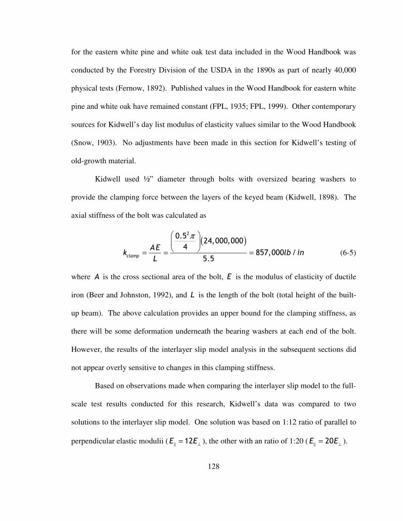
128
for the eastern white pine and white oak test data included in the Wood Handbook was
conducted by the Forestry Division of the USDA in the 1890s as part of nearly 40,000
physical tests (Fernow, 1892). Published values in the Wood Handbook for eastern white
pine and white oak have remained constant (FPL, 1935; FPL, 1999). Other contemporary
sources for Kidwell’s day list modulus of elasticity values similar to the Wood Handbook
(Snow, 1903). No adjustments have been made in this section for Kidwell’s testing of
old-growth material.
Kidwell used ½” diameter through bolts with oversized bearing washers to
provide the clamping force between the layers of the keyed beam (Kidwell, 1898). The
axial stiffness of the bolt was calculated as
( )20.5
24,000,0004
857,000 /5.5
clamp
AEk lb in
L
π = = = (6-5)
where A is the cross sectional area of the bolt, E is the modulus of elasticity of ductile
iron (Beer and Johnston, 1992), and L is the length of the bolt (total height of the built-
up beam). The above calculation provides an upper bound for the clamping stiffness, as
there will be some deformation underneath the bearing washers at each end of the bolt.
However, the results of the interlayer slip model analysis in the subsequent sections did
not appear overly sensitive to changes in this clamping stiffness.
Based on observations made when comparing the interlayer slip model to the full-
scale test results conducted for this research, Kidwell’s data was compared to two
solutions to the interlayer slip model. One solution was based on 1:12 ratio of parallel to
perpendicular elastic modulii ( 12E E⊥=�
), the other with an ratio of 1:20 ( 20E E⊥=�
).

129
6.4.2 Brunel’s Beam
Kidwell fabricated and conducted two tests on what he described as “Brunel’s
beam,” which is based on a design proposed by I.K. Brunel. Brunel’s design included a
built-up beam using inclined white oak shear keys to provide interaction between the
layers. The white oak shear keys were installed as a pair of wedges such that they would
be compressed across the grain. The layers were clamped together using 0.5 inch
diameter bolts. The basic style of this beam is very similar to the full-scale beams tested
in this research using inclined keys. Figure 6-8 shows the layout of the beams tested by
Kidwell. The beams were tested by applying a point load at mid span until ultimate load
was reached. Deflection measurements were taken at midspan in 0.0625 inch increments.
The load-deflection plots of Kidwell’s two tests are included in Figure 6-9. The test
numbering (0F and 0G) used in the figures and tables correspond to his test numbering
procedure.
Figure 6-8 Key configuration in Brunel's beams (Kidwell, 1898)

130
0
500
1000
1500
2000
2500
3000
3500
4000
4500
0 0.1 0.2 0.3 0.4 0.5 0.6 0.7
Deflection (inches)
Lo
ad
(lb
s)
0F
0G
E/12
E/20
Figure 6-9 Load-deflection plots for Brunel's beams (Kidwell, 1898)
The interlayer slip model solution for a single point load (included in Appendix
B) was used to analyze Brunel’s beams. The simplified approach for determining shear
key spacing was used (the summation of all the shear key stiffness over the length of the
beam) for the analysis. The test stiffnesses and calculated stiffness are included in Table
6-5. The interlayer slip calculations can be found in Appendix H.
Table 6-5 Comparison of Brunel's beam stiffnesses to the interlayer slip model
Test Ult. Load Calc. Calculated Test Difference Difference
E||=E┴/12 E||=E┴/20 E||=E┴/12 E||=E┴/20
lb lb/in lb/in lb/in % %
0F 9780 8089 7112 8000 1.1% -12.5%
0G 8660 8089 7112 7500 7.3% -5.5%
Avg. 4.2% -9.0%
Stiffness
As with the full-scale testing conducted specifically for this research, the
interlayer slip model resulted in a slightly stiffer beam than was observed during the

131
physical testing. However, the average difference between the calculated stiffness and
the actual stiffness for these beams was 4.2% using an elastic ratio of 12
EE ⊥=�
and 9.0%
using a ratio of 20
EE ⊥=�
. Looking at the two tests individually, it appears the 1:12 elastic
ratio fits the first test better, whereas 1:20 fits the second test data better, suggesting the
interlayer slip model accurately represents the historical beam tests fairly well, but that
optimal elastic ratio falls somewhere between 1:12 and 1:20.
6.4.3 Joggled Beam
Kidwell conducted additional tests on what he described as a joggled beam (that
is, a beam where the keys are not inclined) (Kidwell, 1898). The key stiffness terms that
were developed in section 2.5 can account for both the inclined keys and the square (non
inchclined) keys. Kidwell conducted five tests on the joggled beams using white oak
shear keys, and an additional two tests on joggled beams using cast iron shear keys. The
configuration of the joggled beams can be seen in Figure 6-10 and Figure 6-11.
Figure 6-10 Key configuration for joggled beam using white oak keys (Kidwell, 1898)

132
Figure 6-11 Key configuration for joggled beam using cast iron keys (Kidwell, 1898)
The interlayer slip model was again employed to compare the theoretical stiffness
of the joggled beams to the observed stiffness. The load-deflection plots of the joggled
beams with white oak keys using Kidwell’s data can be found in Figure 6-12. The
tabulated stiffnesses are in Table 6-6. As before, the stiffness predicted from the
interlayer slip model is slightly higher than observed beam stiffness. Kidwell observed a
substantial defect in the bottom face of beam 23, which he believed caused the reduced
stiffness and premature failure. Excluding this defective beam, the average difference
between the predicted stiffness and the observed stiffness is 7.5%, which again shows the
interlayer slip model appears to be correctly predicting the behavior of built-up wooden
beams. On average, an elastic ratio of 20
EE ⊥=�
appears to best capture the beams’
behavior.
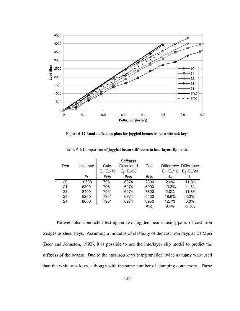
133
0
500
1000
1500
2000
2500
3000
3500
4000
4500
0 0.1 0.2 0.3 0.4 0.5 0.6 0.7
Deflection (inches)
Lo
ad
(lb
s)
20
21
22
23
24
E/12
E/20
Figure 6-12 Load-deflection plots for joggled beams using white oak keys
Table 6-6 Comparison of joggled beam stiffnesses to interlayer slip model
Test Ult. Load Calc. Calculated Test Difference Difference
E||=E┴/12 E||=E┴/20 E||=E┴/12 E||=E┴/20
lb lb/in lb/in lb/in % %
20 10600 7961 6974 7800 2.0% -11.8%
21 6800 7961 6974 6900 13.3% 1.1%
22 8400 7961 6974 7800 2.0% -11.8%
23 5260 7961 6974 6400 19.6% 8.2%
24 8660 7961 6974 6950 12.7% 0.3%
Avg. 9.9% -2.8%
Stiffness
Kidwell also conducted testing on two joggled beams using pairs of cast iron
wedges as shear keys. Assuming a modulus of elasticity of the cast-iron keys as 24 Mpsi
(Beer and Johnston, 1992), it is possible to use the interlayer slip model to predict the
stiffness of the beams. Due to the cast iron keys being smaller, twice as many were used
than the white oak keys, although with the same number of clamping connectors. These

134
variations were taken into account when using the interlayer slip model. Kidwell’s load-
deflection plots are shown in Figure 6-13, with the corresponding stiffness data shown in
Table 6-7.
The interlayer slip model appears to accurately predict the stiffness of the built-up
beams using cast-iron keys, again with elastic ratio of 20
EE ⊥=�
best capturing actual
beam behavior. The interlayer slip model over predicted the stiffness in one case, and
under predicted the stiffness in the other case, although by minimal amounts. The
theoretical upper-bound to this particular test configuration (assuming a full depth solid
beam), is a stiffness of 10,663 lb/in. Therefore, using cast-iron keys, it appears it is
possible to achieve beams nearly as stiff as their full depth counterpart.
0
500
1000
1500
2000
2500
3000
3500
4000
4500
0 0.1 0.2 0.3 0.4 0.5 0.6 0.7
Deflection (inches)
Lo
ad
(lb
s)
28
29
E/12
E/20
Figure 6-13 Load-deflection plots for joggled beams using cast iron keys

135
Table 6-7 Comparison of joggled beam stiffnesses to interlayer slip model
Test Ult. Load Calc. Calculated Test Difference Difference
E||=E┴/12 E||=E┴/20 E||=E┴/12 E||=E┴/20
lb lb/in lb/in lb/in % %
28 10190 10500 10346 10100 3.8% 2.4%
29 11190 10500 10346 10600 -1.0% -2.5%
1.4% 0.0%
Stiffness
6.4.4 Three Layer Beam
The interlayer slip model developed in section 2 was based on a built-up beam
made with n-plies, with specific solutions for a two layer beam in section 2.1.2 and a
three layer beam in section 2.1.3. However, all work using the interlayer slip model after
that point has focused on beams built from two plies. While no physical testing was
conducted on three-layer keyed beams for this research, Kidwell conducted a full scale
test on one, which is the basis for this comparison (Kidwell, 1898).
Kidwell’s test on a three-layer beam (his test number 27), the configuration of
which is shown in Figure 6-14, employed the use of 1 inch by 2 inch white oak shear
keys installed square to the timber being compressed perpendicular to the grain. As with
the joggled beams described above, the shear key stiffness terms already developed are
capable of handling this key configuration.
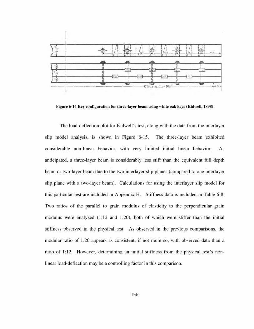
136
Figure 6-14 Key configuration for three-layer beam using white oak keys (Kidwell, 1898)
The load-deflection plot for Kidwell’s test, along with the data from the interlayer
slip model analysis, is shown in Figure 6-15. The three-layer beam exhibited
considerable non-linear behavior, with very limited initial linear behavior. As
anticipated, a three-layer beam is considerably less stiff than the equivalent full depth
beam or two-layer beam due to the two interlayer slip planes (compared to one interlayer
slip plane with a two-layer beam). Calculations for using the interlayer slip model for
this particular test are included in Appendix H. Stiffness data is included in Table 6-8.
Two ratios of the parallel to grain modulus of elasticity to the perpendicular grain
modulus were analyzed (1:12 and 1:20), both of which were stiffer than the initial
stiffness observed in the physical test. As observed in the previous comparisons, the
modular ratio of 1:20 appears as consistent, if not more so, with observed data than a
ratio of 1:12. However, determining an initial stiffness from the physical test’s non-
linear load-deflection may be a controlling factor in this comparison.

137
0
500
1000
1500
2000
2500
3000
3500
0 0.2 0.4 0.6 0.8 1 1.2 1.4
Deflection (inches)
Lo
ad
(lb
s)
27
E/12
E/20
Full
Stacked
Figure 6-15 Load-deflection plots for three-layer beam using white oak keys
Table 6-8 Comparison of three-layer beam stiffness to interlayer slip model
Test Ult. Load Calc. Calculated Test Difference Difference
E||=E┴/12 E||=E┴/20 E||=E┴/12 E||=E┴/20
lb lb/in lb/in lb/in % %
27 5400 4140 3620 3600 13.0% 0.6%
Initial Stiffness
Beams consisting of more than three layers are not discussed in this research for
several reasons. The cumulative effect of in-service moisture related cross-sectional
changes in built-up heavy timber beams made from more than three layers would be very
difficult to address, in particular when ensuring that adequate key-clamping forces could
be maintained. Another limiting factor for excessively deep built-up beams is their
relatively inefficiency for long spans, as a truss system can carry loads considerably more
efficiently than an equivalent depth beam.

138
6.4.5 Discussion of Results
The interlayer slip model appears to predict the behavior of Kidwell’s historical
data quite well. With the equations developed in section 2, it was possible to model both
inclined shear keys (“Brunel’s beam”) and square shear keys (“joggled beams”) made
from various materials. A three-layer beam using white oak shear keys was also
modeled. As was noticed in the full-scale testing of beams for this research, the white
oak keyed beams have more variation in stiffness from one test to another compared to
those with manufactured key material (Parallam PSL or cast-iron wedges). Assuming a
ratio of 1:12 for the parallel-to-grain to perpendicular-to-grain elastic modulii appears to
over predict the stiffness (6.8% stiffer for all of Kidwell’s tests). An assumed elastic
ratio of 1:20, as has been suggested by previous authors (Bodig and Jayne, 1982) slightly
under predicts the beam stiffness (3.6% softer).

139
7 Ultimate Stress
The focus of the physical testing along with the comparisons to the interlayer slip
model up until this point have focused on deflection and stiffness. In order to evaluate
the failure and safe working loads, determining the stress in the layers is required.
7.1 Predication of Failure Load
The flexural stress in a wooden member at the time of a bending failure is
commonly referred to as the modulus of rupture (MOR). The average modulus of rupture
for most species of wood is published in the Wood Handbook (FPL, 1999), or can be
found from small scale testing. For a built-up beam, failure can be described as occurring
when the stress at either the top or bottom face exceeds the material’s modulus of rupture.
That is,
2
2
TT T
BB B
hMOR
hMOR
σ
σ
>
>
(7-1)
where T
h and B
h are the depths of the top and bottom layers, respectively. Similarly, T
σ
and B
σ are the stresses in the top and bottom layers at these points, as calculated from
equations (2-43) and (2-44). For a specific loading configuration, both the moment M
and the axial force in the layers F from composite action can be written as functions of
the applied load. Setting the applied stress equal to the average published modulus of
rupture (rather than the inequality described in equation (7-1)) allows for direct solution
for the anticipated failure load.

140
7.2 Comparison to Full Scale Testing
The extreme fiber stress at the maximum load for each of the four keyed beams
was calculated using the procedure outlined in section 2.4. The stress at maximum load
was calculated using test data from the physical tests (see Table 6-1). Calculations for
determining the stress are included in Appendix I, and the relevant information is
summarized in Table 7-1. The extreme fiber stress for a simple stacked beam as well as a
full depth beam subjected to the applied load are also included as upper and lower limits.
Statistical data is not included, as only tests 1 and 2 showed signs of rupture at the
maximum load (tests 3 and 4 buckled due to inadequate bracing of the hydraulic
actuator).
Table 7-1 Stress at maximum load for full-scale beam tests
Test
Max.
Load Calculated Calculated
Full
Beam
Simple
Beam Published Adjusted
E||=E┴/12 E||=E┴/20 MOR MOR E||=E┴/12 E||=E┴/20
lb psi psi psi psi psi psi % %
1 34130 6213 6669 4252 8503 10100 6898 -9.9% -3.3%
2 39620 6759 7254 4994 9987 10100 7427 -9.0% -2.3%
3* 42370 6012 6109 4685 9370 10100 6974 -13.8% -12.4%
4* 35060 4691 4925 3879 7759 10100 7618 -38.4% -35.3%
* Ultimate load was never reached
Stress @ Max. Load
Calc. vs MOR
The calculated stress is based on the material properties of the timber at the time
of testing, rather than the published values based on a normalized 12% moisture content.
In order to compare the calculated stresses to the published modulus of rupture, the
published modulus of rupture (MOR) values were adjusted following the procedure set
forth in the Wood Handbook (FPL, 1999), which has been used in the previous sections.

141
The anticipated modulus of rupture, ACT
MOR , based on the material’s moisture content
and specific gravity is calculated as
121.0113
12%12% 1.01
12%
MC
ACTACT
GREEN
MOR GMOR MOR
MOR G
−
=
(7-2)
where 12%,GREEN
MOR are the published MORs for wood at 12% moisture content as well as
in the green state, MC is the moisture content of the material, and ,12%ACT
G is the actual
and published oven dry specific gravity of the material. The average moisture content
and specific gravity (shown in Table 6-1) of the top and bottom layers in each test were
used when calculating the anticipated modulus of rupture.
Published modulus of rupture values are based on testing conducted on small,
clear, straight grained samples. However, it has been shown that the strength of beams
decreases as the size increases (FPL, 1999). Therefore, published allowable bending
stress values take into account the cross-sectional size of the timber (AF&PA, 2007). To
account for the larger cross sections used in this research’s testing component,
adjustments were made to the modulus of rupture following the procedure outlined in the
Wood Handbook (FPL, 1999). The adjusted modulus of rupture, ADJ
MOR , was
calculated as
1
22 2
2
11 1
1
1
1
m
ADJ ACT
mah L
LMOR MOR
mahL
L
+
=
+
(7-3)

142
where ACT
MOR is the modulus of rupture from equation (7-2), h and L are the depth of
the test specimens, a is the distance between the symmetrically placed point loads, and
m is a constant, normally taken as 18. The published modulus of rupture values in the
Wood Handbook and other sources are determined according to ASTM D143 (ASTM,
2007), which consists of 2 inch by 2 inch material spanning 28 inch and loaded by a point
load at midspan. Taking this information into account, along with the loading
configuration for the full scale testing, equation (7-3) can be rewritten as
( )
1
1856
810ADJ ACT
T B
MOR MORh h
=
+ (7-4)
where T
h and B
h are the depths of the top and bottom layers of the built up beam. The
adjusted moduli of rupture values are included in Table 7-1.
The extreme fiber stress in the keyed beam was calculated using elastic ratios of
12E E⊥=�
and 20E E⊥=�
, with the 1:20 ratio providing slightly better results than the
1:12 ratio. Statistical data is not included in Table 7-1, as only tests 1 and 2 showed signs
of rupture at the maximum load (tests 3 and 4 buckled due to inadequate bracing of the
hydraulic actuator). However, based on this limited amount of data, it appears the
interlayer slip model appears to be accurately predicting the extreme fiber stress.
7.3 Comparison to Kidwell’s Historical Testing
In order to further investigate the accuracy of the interlayer slip model at
predicting the extreme fiber stress at rupture, Kidwell’s test data was also analyzed in a
fashion similar to section 7.2. The results of the analysis are included in Table 7-2.

143
Moisture content and specific gravity information was not available for Kidwell’s test
data, and his physical tests were conducted on small beams, so no adjustments to the
published modulus of rupture were made. Kidwell noted a substantial defect in test 23,
which he believed caused its premature failure.
Table 7-2 Stress at maximum load for Kidwell’s beam tests
Test
Max.
Load Calc. Calculated
Full
Beam
Simple
Beam Published
E||=E┴/12 E||=E┴/20 MOR E||=E┴/12 E||=E┴/20
lb psi psi psi psi psi % %
0F 9780 8592 9333 6738 13477 8600 -0.1% 8.5%
0G 8660 7608 8264 5967 11933 8600 -11.5% -3.9%
20 10600 9552 10115 7303 14607 8600 11.1% 17.6%
21 6800 6128 6489 4685 9370 8600 -28.7% -24.5%
22 8400 7570 8016 5788 11575 8600 -12.0% -6.8%
23 5260 4740 5020 3624 7248 8600 -44.9% -41.6%
24 8660 7804 8264 5967 11933 8600 -9.3% -3.9%
28 10190 8428 8721 7021 14042 8600 -2.0% 1.4%
29 11190 9254 9578 7710 15420 8600 7.6% 11.4%
Avg* -5.6% 0.0%
* Test 23 Data Removed
Calc. vs MOR
Stress @ Ultimate
The extreme fiber stress in Kidwell’s beams were calculated using elastic ratios of
12E E⊥=�
and 20E E⊥=�
, again with the 1:20 ratio providing slightly better results than
the 1:12 ratio. Based on these findings, the interlayer slip model appears to accurately
predict the failure stress of a keyed beam.
7.4 Discussion of Results
As can be seen in Table 7-1 and Table 7-2, using the interlayer slip model appears
to be a viable method to calculate the failure stress in a beam with partial interaction
between layers. As has been observed in the previous sections, an elastic ratio where

144
20E E⊥=�
appears to best represent the beam behavior, based both on stiffness and on
strength criterion.
For the test configurations used, the maximum stress occurs at the applied point
loads (recall Figure 2-6). Any defect near these points can increase the likelihood of
stress concentrations, which are not captured by the interlayer slip model. Although the
second full scale test showed cracks propagating from the reentrant corner of the shear
key notches nearest the applied point load (Figure 5-8), these stress concentrations did
not appear to have any impact on the beam capacity.

145
8 Design Procedure
The interlayer slip model developed in section 2 appears to predict the behavior of
actual keyed beams quite well (section 6). For common design situations, the exact
material properties of each individual piece of material used in a built up beam will not
be known, and the size and configuration of shear keys will need to be developed.
Therefore, a method for determining a design capacity of a particular configuration from
readily available published design information is required.
The design of a built-up keyed beam is an iterative process. The size and number
of layers in the built up beam needs determined. Likewise, the number and type of shear
keys, their spacing, and the number of clamping connectors needs to be chosen before the
beam can be analyzed. After the initial analysis, the timber sizes and shear key
components can be adjusted accordingly, followed by a re-analysis of the beam.
8.1 Shear Key and Clamping Connector Design
Design of a shear key and clamping connector is based on the force being
transferred between the layers of the built-up beam. Exact and simplified methods for
analyzing the stress and stiffness of a built up beams are detailed in subsequent sections.
However, determination of the capacity of the shear keys and clamping connectors
should follow the same proceedure, regardless of whether an exact or simplified
procedure is used for the design of the beam.

146
8.1.1 Shear Key and Timber Compressive Strength
The capacity of a shear key can be limited by either the compressive capacity of
the shear key or the compressive capacity of the timber at the shear key notch. Using the
notation shown in Figure 2-8, the horizontal shear capacity N of a key is
,
,
'min
'
c key
c tim
btFN
btF= (8-1)
where b is the lesser breadth of the two layers being connected by the shear key and t is
the depth of the notch perpendicular to the interface. ,
'c key
F and ,
'c tim
F are the adjusted
allowable compressive stresses in the key and timber, respectively, determined in
accordance with section 4 of the National Design Specification for Wood Construction,
henceforth referred to as the NDS (AF&PA, 2005). The NDS includes published
allowable compressive, shear, tensile, and bending stress values, determined following
the appropriate ASTM standards depending on size and material, along with adjustment
factors for variations in anticipated in-service moisture content, size, and temperature.
These adjustments apply to a built-up beam in a similar fashion to a solid or simply
stacked beam.
When calculating ,
'c key
F for a key installed such that it is being compressed
perpendicular to the grain, all of the adjustment factors included in the NDS should
apply. For ,
'c key
F when the key is being compressed parallel to the grain as well as all
instances of ,
'c tim
F , all adjustment factors apply except for the column stability factor.
Solid sawn shear keys should be made from clear, straight grained material (see 3.1.2),

147
and thus tabulated allowable stresses for select structural material should be used for the
keys.
8.1.2 Shear Key Spacing
The minimum spacing between shear keys is determined by the material
properties and key configuration, and is independent of the external load that is applied to
the beam. The spacing is determined by ensuring there is adequate shear resistance
between the shear key notches to develop the full design capacity of the shear key. The
NDS includes a non-mandatory suggestion to use a more conservative linear shear stress
distribution (AF&PA, 2005) (see section 3.6), although common design practice in
timber construction is to use a less conservative uniform stress distribution (Goldstein,
1999). For a shear key designed to resist a horizontal shear force N (Figure 2-8), the
minimum shear key spacing is
min
'V
Ns
bF= (8-2)
where 'V
F is the adjusted allowable horizontal shear strength of the timber, calculated in
accordance with section 4 of the NDS (AF&PA, 2005).
The maximum spacing between shear keys can be determined by using the shear
flow q for a beam. The maximum spacing, maxs , can be found by setting the shear key
capacity equal to the area under the shear flow diagram and solving for the horizontal
spacing. The maximum spacing is therefore dependent on the applied load, as different
moment distributions result in different shear distributions. A solid beam of uniform

148
cross section along the length has a constant first moment and moment of inertia, so the
shape of the shear diagram accurately depicts the shape of the shear flow diagram.
For a beam with a pair of equal, symmetrically placed concentrated loads, the
moment distribution is linear and the shear diagram is constant at the ends, with constant
moment and no shear in the middle (see Figure 3-7). Using the shear flow diagram for a
solid beam to approximate for the shear flow diagram for a built up beam, the maximum
shear key spacing is therefore constant along the end sections based on the area under the
shear flow diagram (Figure 8-1a). A beam subjected to a uniformly distributed load has a
parabolic moment distribution and linear shear distribution about the entire length. The
linear distribution of shear (and thus shear flow) results in a larger maximum shear key
spacing near the middle of the span than near the ends (Figure 8-1b).

149
q
q
s
Area = qs = N
max
maxN N
N N N
(a)
N N
NNN
Area = N
sss1 2 3
q
(b)
Figure 8-1 Shear key spacing for a beam with (a) two concentrated point loads, and (b) a uniformly
distributed load.
For a built-up beam that has full composite action between the layers, equation (2-
58) can be used to determine the shear key spacing. However, a built-up beam has only
partial composite action between the layers, the shear force is determined by the
differential equation described in equation (2-14), where the shear force is determined by
the change in axial force about the length. Therefore, the maximum shear key spacings
determined from the shear flow curve of the full-depth beam will vary slightly from the
spacings determined from the built-up beam shear flow curve). As the area under the
full-depth beam curve is always greater than the built-up beam curve (see Figure 2-12a

150
and Figure 2-12b, use of the shear flow diagram for from a full depth beam to determine
shear key spacing for design purposes appears adequate and slightly conservative.
8.1.3 Clamping Strength Requirements
Sufficient clamping connector strength should be used to generate the full design
compressive capacity of the shear keys. The sensitivity analysis conducted in section
6.3.3 suggests that excessive clamping connector stiffness has a diminishing benefit on
the stiffness of a built-up beam, so specifying additional connectors beyond the design
capacity of the shear keys appears to be an inefficient method of increasing built-up beam
performance.
The minimum required clamping force, R , is found by summing moments about
the point of rotation in a shear key (see Figure 8-2 and Appendix D), such that
Nt
Rw t
=+
(8-3)
where N is the horizontal capacity of the shear key, t is the depth of the shear key notch
perpendicular to the interface, and w is the length of the shear key parallel to the
interface. Equation (8-3) is based on the clamping connector being installed a distance t
away from the shear key notch, which is shown Figure 8-2.
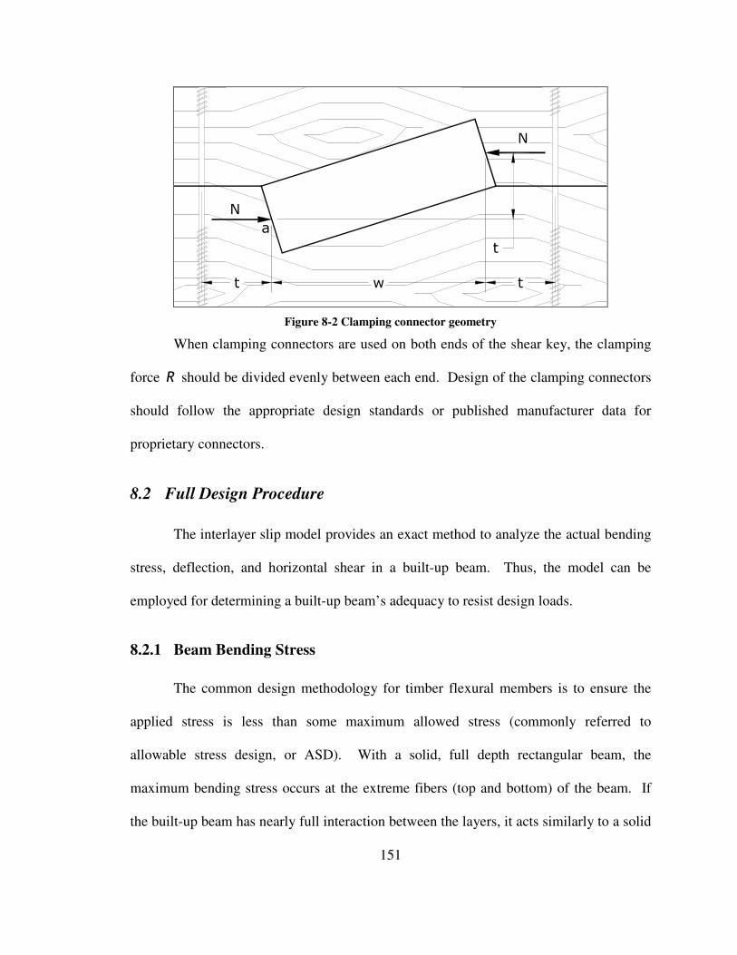
151
N
N
t
w
a
tt
Figure 8-2 Clamping connector geometry
When clamping connectors are used on both ends of the shear key, the clamping
force R should be divided evenly between each end. Design of the clamping connectors
should follow the appropriate design standards or published manufacturer data for
proprietary connectors.
8.2 Full Design Procedure
The interlayer slip model provides an exact method to analyze the actual bending
stress, deflection, and horizontal shear in a built-up beam. Thus, the model can be
employed for determining a built-up beam’s adequacy to resist design loads.
8.2.1 Beam Bending Stress
The common design methodology for timber flexural members is to ensure the
applied stress is less than some maximum allowed stress (commonly referred to
allowable stress design, or ASD). With a solid, full depth rectangular beam, the
maximum bending stress occurs at the extreme fibers (top and bottom) of the beam. If
the built-up beam has nearly full interaction between the layers, it acts similarly to a solid

152
beam. Likewise, if the built-up beam has limited action between the layers, it acts
similarly to two stacked beams, which have similar stresses on the top and bottom of each
layer. Therefore, the maximum stress will always occur on the top and bottom faces of a
two-layer beam, assuming no material defects or other discontinuities that can cause
stress concentrations.
For a two layer built-up beam with partial interaction, equations (2-43) and (2-44)
can be used to evaluate the stress at any point. The process outlined in section 2.4 can be
used for beams with additional layers. Using these equations, the extreme fiber bending
stress in the top and bottom layers, bf , can be compared to the maximum adjusted
allowable bending stress, 'b
F , such that
'b bf F≤ (8-4)
where 'b
F is determined using section 4 of the NDS (AF&PA, 2005), and the tabulated
bending stress is based on the lowest bending stress of an individual layer. For the size
adjustment factor, using the cross sectional area of the full depth beam is slightly
conservative compared to that of a simply stacked beam or some other equivalent depth
beam. Using the lateral-torsional stability factor for the full depth beam is suggested,
although it is slightly unconservative for a partially composite beam, as there is not full
lateral interaction between layers. For common design configurations, the clamping
connectors required to resist shear key rotation should provide sufficient lateral restraint
to cause the beam to act rigidly in torsion.

153
8.2.2 Beam Stiffness
As discussed in detail in section 6, the interlayer slip model can accurately predict
the stiffness of actual built-up beam using wood keys. For design purposes, using the
published modulus of elasticity values from the NDS for determining the beam and key
stiffness is consistent with the design procedures for solid sawn beams. As with the
bending stress, the modulus of elasticity is adjusted for variations in moisture content and
temperature, resulting an adjusted modulus of elasticity value, 'E , used in calculating
beam deflections. These adjusted elastic moduli can be used with the interlayer slip
model to predict the actual keyed-beam deflection, which can be compared to
serviceability requirements outlined in the governing building code.
8.3 Simplified Design Procedure
While the interlayer slip model can be used for design purposes, solving the
governing differential equations and analyzing each individual solution for new loading
conditions is impractical if built up beams are to be used in regular design practice. An
approach that provides a similar level of performance with reduced effort is therefore
desired.
To predict the stiffness of a built-up beam, the Eurocode (2004) uses an
approximation based on an effective “EI” (modulus of elasticity multiplied by the
moment of inertia), which is described in further detail by Thelandersson and Larsen
(2003). This method is based on a sinusoidal loading condition with a uniform connector
spacing, where the connector shear stiffness is known. The approach of using an
effective “EI” is analytically quite convenient as it allows for the use of existing

154
structural analysis methods for a solid timber cross section to be used. For keyed beams
made from similar species of wood, the modulus of elasticity will be the same for all
layers, so an effective moment of inertia is able to capture the interlayer slip’s effect on
beam stiffness. Expansion of the Eurocode method is investigated in this research a
possibility for keyed beams.
For a stacked beam with no interaction between the layers, the moment of inertia
of the combined beam of n layers is
1
n
stacked ii
I I=
=∑ (8-5)
where iI is the moment of inertia for the ith layer. Using the parallel-axis theorem, the
moment of inertia for a built-up beam with full interaction between the layers (e.g. a full
depth beam) is
2
1 1
n n
full i i ii i
I I Ad= =
= +∑ ∑ (8-6)
where i
A is the cross-sectional area and i
d is the distance from the centroid of the built-
up beam to the centroid of the ith layer. The moment of inertia of a built-up beam with
partial interaction will have a moment of inertia that falls somewhere between that of a
stacked and full depth beam, such that
2
1 1
n n
eff i i ii i
I I Adλ= =
= +∑ ∑ (8-7)
where λ is some number between 0 (simple stacked beam) and 1 (full-depth beam), and
is the efficiency of the keys at providing interaction between the layers (see section 2.6).
Individual solutions of the interlayer slip model for a given loading configuration can
155
yield closed form solutions for λ if the shear key stiffness and spacing is known.
However, development of a method for calculating a simplified λ is not included in this
research due to the limited number of physical tests from which to draw conclusions.
The lateral-torsional buckling adjustment to the tabulated allowable design
bending stress included in the NDS does not include a moment of inertia term. To allow
for use of this term, the effective EI discussed above should be adjusted to account for the
reduced beam stiffness entirely in the modulus of elasticity term. This change can be
accounted by the relationship
full eff eff full
E I E I= (8-8)
where full
E is the tabulated modulus of elasticity of the timber, eff
E is an effective
modulus of elasticity of the beam for use in the beam lateral-torsional stability adjustment
factor calculations, and fullI is the full depth moment of inertia of the beam.

156
9 Conclusions
9.1 Summary
The main focus of this research was to investigate whether the traditional
interlayer slip model, in conjunction with a shear key stiffness model, would be able to
accurately predict the strength and stiffness of a built up keyed beam that has partial
interaction between layers. To verify this hypothesis, solutions of the governing
interlayer slip differential equations were developed for several common loading
configurations, small scale testing was conducted to determine key and connector
stiffness parameters, and full scale beam testing was also conducted. Test data from
historical sources was compared to solutions of the interlayer slip model.
Based on the findings from the investigations conducted as part of this research,
several significant contributions were made to the field of interlayer slip analysis and
timber engineering. Specifically,
- the interlayer slip model was expanded to include the ability to model any
n-layer beam.
- the interlayer slip model’s ability to accurately model keyed beam
behavior was verified through comparison to full-scale tests.
- an analytical model was developed that captured the stiffness behavior of
various shear key assemblies.
- a robust analytical design procedure was developed allowing for the
design and analysis of keyed beams made with various key configurations
and subjected to different loading conditions.

157
9.2 Qualified Recommendations
Based on observations made and data collected during this research, several
recommendations can be made about the behavior or design of keyed beams. These
recommendations are intended for engineers and fabricators that design and build keyed
beams.
- When shear keys made from solid wood are used, they should be installed
such that they are compressed perpendicular to the grain. While the
perpendicular to the grain compressive stiffness of wood is considerably
less than the parallel to the grain compressive stiffness, ease of installation
of the shear key wedges makes up for this shortcoming. Installing the
shear keys such that they are compressed parallel to the grain can easily
result in damaged keys (see Figure 3-2). Keys made from manufactured
material, such as Parallam PSL, can be easily installed such that they are
compressed parallel to the grain, and thus are considerably more efficient
than an equivalent sized solid sawn shear key.
- For yellow poplar and white oak, using an elastic ratio of 1:20 (i.e.,
20E E⊥=�
) appears to best model actual timber behavior. As yellow
poplar acts more like a softwood (despite being classified as a hardwood)
and white oak is representative of most hardwoods used in heavy timber
construction, an elastic ratio of 1:20 should be used for other species as
well.

158
- Shear key stiffness has a strong impact on overall beam efficiency and
stiffness. Therefore, using shear keys with higher compressive stiffnesses
will result in higher beam stiffnesses. However, shear key compressive
stiffnesses that greatly exceed the bearing stiffness of the timber (such as
cast-iron keys) at the shear key notch provide diminishing returns on beam
efficiency.
- All shear keys require a clamping mechanism in order to resist rotation
when loaded. Several options exist for clamping connectors, as is
discussed in detail in section 3.3. However, overly stiff or an excessive
number of clamping connectors does not have a substantial effect on
keyed beam efficiency or stiffness. Enough clamping capacity should be
provided such that the shear key is more likely to compress than rotate;
any additional clamping capacity beyond this point has limited benefit (see
section 6.3.3).
- Inclined shear keys are preferable to square shear keys, in that they require
substantially less key material, which in turn results in less material being
removed for shear key notches in the main timbers. With modern cutting
tools, making inclined shear key notches requires a similar level of effort
as square shear key notches. Inclined shear keys also are in pure
compression, whereas square shear keys are subjected to compression as
159
well as shear. However, inclined shear keys can only resist slipping in one
direction.
- Concentrated loads can cause spikes in the extreme fiber bending stress of
the timber layers (see Figure 2-6). Before notches are placed at or near the
point loads, care should taken to ensure the notches will not generate
extensive stress concentrations that cause premature failure of the beam.
- The friction between the layers of a built up beam can be ignored for
analysis purposes. Even when layers were clamped tightly together before
being screwed together, slippage of the layers occurred before any
extensive amount of frictional forces could be developed. Dynamic
friction forces also appear to be negligible.
- The efficiency of built-up beams using more than three plies is quite low,
and does not lend itself to practical use. Parallel chord trusses or other
framing options should be investigated for use in place of keyed beams
requiring more than three layers.
- Double-threaded screws used as clamping connectors ensure tight bearing
of the mating slippage planes. However, the varying pitch on the threaded
portions that pulls the members together does not appear to substantially
affect the axial stiffness of the clamping connector.

160
- The efficiency of built-up beams carrying transverse loads is directly
related to the stiffness of the connecting shear keys. While wood
increases in stiffness as it dries, it also shrinks. Any shrinkage in the shear
keys or in the timbers will negatively impact the capacity and stiffness of
the beam. Therefore, kiln-dried key stock should be used, along with well
dried timbers, whenever possible.
9.3 Future Research
Several areas requiring additional study became apparent during the development
of this research and are listed in below.
- Additional full scale physical testing of keyed beams using various timber
species and key materials, along with different loading configurations and
key grain orientations, are critical. Additional tests will further verify the
interlayer slip and shear key stiffness model’s ability to model the
behavior of built up beams. More testing will also allow for meaningful
statistical analyses to be made, which are required for determining the
reliability of this type of building system.
- While solutions to the interlayer slip model were developed for several
common loading configurations, developing a less computationally
intensive method of predicting beam efficiency is important for continued

161
use by design professionals. Developing a simplified procedure should be
conducted in conjunction with, or after, additional full scale testing, to
lend statistical significance to the procedure.
- Inclined white oak and Parallam PSL shear keys were used in this
research, which proved to be easy to fabricate and install. To further
examine the breadth of applicability of the shear key stiffness model,
testing should be conducted using different materials and key
configurations. The effectiveness of shear keys installed square to the
timber (see Figure 2-7a) at resisting two way slippage (due to reversal of
beam loading) should also be investigated.
- The use of larger shear keys, such that the individual layers of the beam
are spaced some distance apart (no contact between layers), should also be
investigated. While larger (thicker) shear keys increase the clamping
capacity required to keep the keys from rotating, spacing the layers of the
beams apart increases the effective depth with limited increase in material
usage.
- The long term loading of wood, especially members that are subjected to
drying in service, results in measurable amounts of creep. Built-up beams,
in particular ones that use shear keys, can be subjected to fairly high in-

162
service stresses. Therefore, creep of the shear keys as well as the timbers
should be investigated
- Using shear keys fabricated from a pair of opposing wedges allows for
substantial adjustments to the shear key widths, which can account for
fabrication tolerances in the shear key notch sizes. Prestressing and
inducing positive camber into the beams by intentionally mis-aligning
shear key notches, which can then be realigned by driving the shear keys,
is of particular personal interest and should be investigated both from a
theoretical as well as physical standpoint.
- An investigation into the appropriateness of the NDS provisions for lateral
stability of a built-up beam should also be investigated. A partially-
composite beam will not behave the same as a full-depth beam during
lateral-torsional buckling.
- Use of the interlayer slip model to analyze a built-up beam made with
specific cross sectional and material properties, along with a known key
configuration, is fairly straight forward. However, designing the optimal
keyed beam from scratch for a specific loading configuration requires
evaluating many different beam configurations and comparing the results.
An automated procedure for developing the optimal key configuration and
beam parameters based on the designer’s or fabricator’s preference would

163
be extremely valuable. For example, an optimization sequence would
determine if adding more shear keys to a beam is more cost efficient, from
both a labor and material standpoint, than using fewer shear keys and
slightly larger timber cross sections.

164
10 References
American Forest and Paper Association (AF&PA). (2005). “National design
specification for wood construction,” AF&PA, Washington, DC.
ASTM. (2007). 2007 Annual Book of ASTM Standards, 04.10 Wood, Philadelphia, PA.
Benson, T. (1999). Timberframe. Taunton Press, Newtown, CT.
Beer, F.P. and Johnston, E.R. (1992). Mechanics of materials, 2nd
Ed, McGraw-Hill,
New York.
Bodig, J., and Jayne, B.A. (1982). Mechanics of wood and wood composites, Van
Nostrand Reinhold Publishing, New York.
Brungraber, B. (2008). Personal communications.
Coduto, D. (2001). Foundation design, 2nd
Ed, Prentice Hall, Upper Saddle River, NJ.
Cowper, G.R. (1966). “The shear coefficient in Timoshenko’s beam theory,” ASME
Journal of Applied Mechanics, June:335-340.
Dall’Asta, A. and Zona, A. (2004). “Slip locking in finite elements for composite beams
with deformable shear connection,” Finite Elements in Analysis and Design,
40:1907-1930.
Durm, J., and Esselborn, K. (1908). Lehrbuch des Hochbaues, Wilhelm Engelmann,
Leipzig.
Eurocode. (2004). “Eurocode 5: Design of timber structures,” EN 1995-1-1:2004(E).
Faella, C., Martinelli, E., and Nigro, E. (2002). “Steel and concrete composite beams
with flexible shear connection: “exact” analytical expression of the stiffness
matrix and applications,” Computers and Structures, 80:1001-1009.

165
Fernow, B.E. (1892). “Timber Physics,” Forestry Division Bulletins 6&8, United States
Department of Agriculture, Washington, DC.
Forchheimer. (1892). “Ueber zusammengesetzte Balken,” Zeitschrift des Vereines
deutscher Ingenieure, 36:100-103.
Forest Service. (1985). “Yellow poplar,” FS-272, United States Department of
Agriculture, Washington, DC.
Frangi, A. and Fontana, M. (2003). “Elasto-plastic model for timber-concrete composite
beams with ductile connection,” Structural Engineering International, 12(1):47-
57
Forest Products Laboratory. (1935). Wood handbook: basic information on wood as a
material of construction with data for its use in design and specifications, USDA
Forest Service, Madison, WI.
Forest Products Laboratory. (1999). Wood handbook, FPL-GTR-113, Madison, WI.
Goldstein, E.W. (1999). Timber construction for architects and builders, McGraw-Hill,
New York.
Goodman, J.R. (1967). “Layered wood systems with interlayer slip,” Ph.D.
Dissertation. University of California, Berkley.
Goodman, J.R. and Popov, E.P. (1968). “Layered beam systems with interlayer slip,”
Journal of the Structural Division, ASCE, Nov:2535-2547
Granholm, H. (1949). “Om sammansatta balkar och pelare med sarskild hansyn till
spikade trakonstrucktioner,” Transactions, Chalmers Tekniska Hogskolas
Handlingar, No. 88. Gottenburg, Sweden.

166
Gromala, D.W. (1985). “Determination of modulus of rigidity by ASTM D 198 flexural
methods,” ASTM Journal of Testing and Evaluation, 13(5):353-355.
International Code Council (ICC). (2006). 2006 International Building Code, ICC.
Falls Church, VA.
International Code Council Evaluation Service (ICC-ES). (2007). “Structural composite
lumber,” ESR-1387, Whittier, CA.
Jacoby, H. (1909). Structural details or elements of design in heavy framing, John
Wiley and Sons, New York.
Karlsen, G.G. (1967). Wooden structures, Goodman, W.L., trans. Mir Publishers,
Moscow.
Karlsen, G., & Slitsskouhov, Y. (1989). Wooden and plastic structures, Kuznetsov,
A.B., trans. Mir Publishers, Moscow.
Kidwell, E. (1898). “The efficiency of built-up wooden beams,” Transactions,
American Institute of Mining Engineers, 2/97-7/97:732-818, 977-993.
Leupold, J. (1726). “Theatrum pontificiale: oder Schauplatz der Bruecken und Bruecken-
Baues,” Leipzig.
Mahan, D.H. (1886). A treatise of civil engineering, John Wiley & Sons, New York.
Maple (2007). Maple Software, vs 11.02.330022. Maplesoft, Waterloo, ON.
Newmark, N.M., Siess, C.P., and Viest, I.. M., (1951). “Tests and analysis of composute
beams with incomplete interaction,” Proceedings, Society for Experimental
Stress Analysis, Vol 9., No. 1.
Newmark, N.M. (1959). “A method of computation for structural dynamics,” Journal of
the Engineering Mechanics Division, ASCE, Vol. 85:67-94.

167
Pleshkov, P.F. (1952). “Teoriia rascheta dereviannykh sostavnnykh sterzhnei,”
Moscow.
Rankine, W.J.M. (1889). A manual of civil engineering, 17th
Edition. Charles Griffin
& Company, London.
Ranzi, G. and Bradford, M.A. (2006). “Time-dependent analysis of composite beams
with partial interaction using the direct stiffness approach,” UNICIV Report R-
423, University of New South Wales, Australia.
Ranzi, G. and Bradford, M.A. (2007). “Direct stiffness analysis of a composite beam-
column element with partial interaction,” Computers and Structures, 85:1206-
1214.
Ranzi, G., Gara, F., and Ansourian, P. (2006). “General method of analysis for
composite beams with longitudinal and transverse partial interaction,” Computers
and Structures, 84:2373-2384.
Schnabl, S., Saje, M., Turk, G., and Planinc, I. (2007). “Analytical solution of two-
layer beam taking into account interlayer slip and shear deformation,” Journal
of Structural Engineering, 133(6):886-894.
Snow, C.H. (1903). The principal species of wood: their characteristic properties. John
Wiley & Sons, New York.
Snow, J.P. (1895). “Wooden bridge construction on the Boston and Maine railroad,”
Journal of the Association of Engineering Societies, 14:500-512.
Strukel, M. (1900). Der Brückenbau, O.W. Backman, Kuopio, Finland.
Timber Frame Business Council (TFBC). (2009). Retrieved March 17, 2009, from TFBC
Website: http://www.timberframe.org/

168
Trautwine J.C. (1862). Civil engineer’s pocket book, John Wiley & Sons, New York.
Tredgold, T. (1820). Elementary principles of carpentry, E&F.N. Spon, London.
Thelandersson, S. and Larsen, H.J. (2003). Timber engineering, John Wiley & Sons,
West Sussex, England
Wangaard, F.F. (1981). Wood: Its structure and properties, Penn State University,
University Park, PA.
Wang, Y.C. (1998). “Deflection of steel-concrete composite beams with partial shear
interaction,” Journal of Structural Engineering 124(10):1159-1165
Warren, W.H. (1910). “Engineering construction in steel and timber,” 2nd
Edition, Vol
1. Longmans, Green, and Co., London.
Wheat, D.L. and Calixto, J.M. (1994). “Nonlinear analysis of two-layered wood
members with interlayer slip,” Journal of Structural Engineering, 120(6):1909-
1929.

169
Appendix A – Solution for Two-Layer Beam with a Uniformly
Distributed Load
Shear Flow:
( )( )( )
( )( ) ( )32
cosh( ) sinh 1 cosh
2sinh
FM M
F F
FF F
C xC w C wq x C x C L L x
CC C L
= + − + −
Deflection:
( )( )
( ) ( )( )
( )
( ) ( )
( )
3 42
23 4
2
2
sinhsinh
6 12
( ) * 22 sinh
6 12
sinh
12
M B T F F
F
F
M B T F
F F B B T T
F
M B T F
F
F M B T M B
C h h C L C xC L
C
Lx xC h h C x
wx
C C L E I E ILx x
C
C h h C x
C
wLx L C C h h C h h
+ − +
+ − − ∆ = − +
− − + +
+ − ++
( )( )( )
( )( )
2 2
2 3
2
48 2
T F M B T
F B B T T F B B T T
L C wC h h
C E I E I C E I E I
− ++
+ +

170
Appendix B – Solution for Two-Layer Beam with Point Load at any
Point
For a simply supported beam subjected to a point load, there will be a
discontinuity in the moment diagram, requiring two moment equations to describe the
moment about the length. If the first point load is at a distancea from the starting (e.g.
left) end on a beam with lengthL , the moment equations are
( 0.. ) 1L
aM x a P x
L
= = −
( )( .. ) 1R
aM x a L P x P x a
L
= = − − −
(B-1)
We will also have two governing differential equations that we will need to solve in order
to find the axial force at any point along the length which are
2
2
( )( ) ( )R
F R M R
d F xC F x C M x
dx− = −
2
2
( )( ) ( )L
F L M L
d F xC F x C M x
dx− = − (B-2)
Solving the above system of equations will yield four integration constants (two per
equation). We know the axial force in the layers at the start and end must be zero so
(0) 0L
F =
( ) 0R
F L = (B-3)
We also know the axial force just to the left and right of the point load needs to be the
same, such that
( ) ( )L R
F a F a= (B-4)

171
Likewise, the rate of change of axial force to the left and right of the point load also
needs to be the same, which means
( ) ( )
L RdF a dF a
dx dx= (B-5)
Thus we have found boundary which allows us to solve for the four integration constants.
Source code for Maple 11 (Maple, 2007)
>
>
>
>
>
>
>
>

172
Recognizing the trigonometric functions cosh( )x and sinh( )x we can write these as
>
Solutions for the shear flow at any point can be found by differentiating the force
equations with respect to their position along the length
>
The deflection at any point can be found by solving the equations

173
2
2
2
2
( ) ( )( ) 2 2
( ) ( )( ) 2 2
B TL L
L
B B T T
B TR R
R
B B T T
h hM x F x
d x
E I E Idx
h hM x F x
d x
E I E Idx
− + ∆ =
+
− + ∆ =
+
(B-6)
with the boundary conditions
(0) 0L
∆ =
( ) 0RL∆ =
( ) ( )L RL a L a∆ − = ∆ −
( ) ( )L R
d dL a L a
dx dx∆ − = ∆ − (B-7)
The solution for the axial forces at any point is bounded on the low end with no
axial force, which is consistent with a simple stacked beam. On the upper end, they are
bounded by the case of a solid full depth beam. Reducing the force equations above is
not a simple task, so compatibility with the lower and upper bound requirements is done
by example.
The axial force at any point can be calculated for a full depth beam as the volume
of the stress block in the compression (or tension) zone, with the compression and tension
zones being equal in magnitude. The compression force in top half of a full depth beam,
the total compression force C can be calculated as
2
bF hb
C = (B-8)
where b
F is the extreme fiber bending stress, b is the beam breadth, and h is the depth
from the extreme fiber in compression to the neutral axis. The extreme fiber bending

174
stress can be calculated as
3(2 )
12
b
MhF
b h=
(B-9)
where M is the applied moment. For a point load P at the midspan of a beam with
length L , we can combine equations B-8 and B-9 as
3
16
PLC T
h= = (B-10)
For a beam with the parameters:
100
50
10000
10T B
L
a
P
h h
=
=
=
= =
the compression (or tension) in the top and bottom portions of the beams is 18,750 lb.
Recalling the equations (2-18) and (2-19) for F
C and M
C respectively, they can be
rewritten with the above beam parameters as
2
25F
kC = (B-11)
3
500M
kC = (B-12)
where k is the total stiffness of the shear keys, assuming s (shear key spacing) and E
(modulus of elasticity) are constant.
Using our interlayer slip solution above, we can apply very small and very large
k values to account for a condition with no interlayer stiffness and for full interlayer
stiffness, and calculate the corresponding forces in each layer. These calculated forces

175
correspond exactly with the simple stacked condition (no axial force) and the full depth
condition (18,750-lb).
>
>
>
>

176
Appendix C – Solution for Two-Layer Beam with Symmetrically Placed
Point Loads
For a beam with two point loads, there will be two discontinuities in the moment
diagram, requiring three moment equations to describe the moment about the length. If
the first point load is at a distancea from the starting end, the second point will thusly be
L a− away from the starting end for a beam with lengthL . The moment equations are
1( 0.. )M x a Px= =
2( .. )M x a L a Pa= − =
3( .. ) ( )M x L a L Pa P x L a= − = − − + (C-1)
We will also have three governing differential equations that we will need to solve in
order to find the axial force at any point along the length which are
2
2
( )( ) ( )i
F i M i
d F xC F x C M x
dx− = − (C-2)
where 1,2,3i = . Solving the above equation will yield six integration constants (two per
equation). We know the axial force in the layers at the start and end must be zero so
1(0) 0F =
3( ) 0F L = (C-3 & 4)
W also know the axial force just to the left and right of each point load needs to be the
same, such that
1 2( ) ( )F a F a=
2 3( ) ( )F L a F L a− = − (C-5 & 6)

177
Likewise, the rate of change of axial force to the left and right of each point load also
needs to be the same, which means
1 2( ) ( )dF a dF a
dx dx=
32( )( ) dF L adF L a
dx dx
−−= (C-7 & 8)
Thus we have six boundary conditions without invoking symmetry of the structure,
which allows us to solve for the six integration constants.
Source code for Maple 11 (Maple, 2007) >
> >
>
>
>
> >
> >

178
>
>
>

179
Solutions for the shear flow and deflection at any point can be found by using the
equations
( )
( ) ii
dF xq x
dx= (C-9)
2
2
( ) ( )( ) 2 2
B Ti i
i
B B T T
h hM x F x
d x
E I E Idx
− + ∆ =
+ (C-10)
The solution for the axial forces at any point is bounded on the low end with no axial
force, which is consistent with a simple stacked beam. On the upper end, they are
bounded by the case of a solid full depth beam. Reducing the force equations above is
not a simple task, so compatibility with the lower and upper bound requirements is done
by example.

180
For a beam with the parameters:
100
25
10000
10T B
L
a
P
h h
=
=
=
= =
The axial compressive or tensile force in a full depth beam anywhere in the constant
moment (middle span) region as
3
18,7504
PaC T lb
h= = = (C-11)
Using the relationships for F
C and M
C outlined in equations B-11 and B-12 respectively,
we can evaluate the interlayer slip model, which yields identical forces in each layer.
> >

181
> >
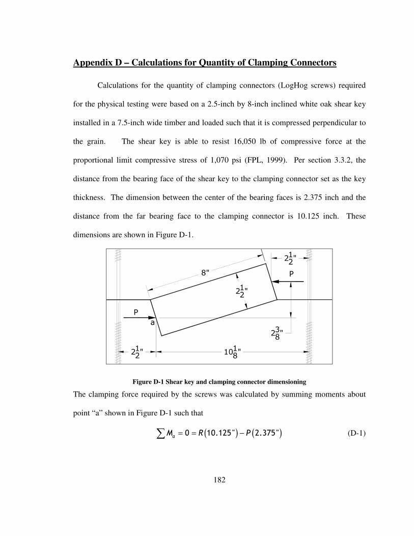
182
Appendix D – Calculations for Quantity of Clamping Connectors
Calculations for the quantity of clamping connectors (LogHog screws) required
for the physical testing were based on a 2.5-inch by 8-inch inclined white oak shear key
installed in a 7.5-inch wide timber and loaded such that it is compressed perpendicular to
the grain. The shear key is able to resist 16,050 lb of compressive force at the
proportional limit compressive stress of 1,070 psi (FPL, 1999). Per section 3.3.2, the
distance from the bearing face of the shear key to the clamping connector set as the key
thickness. The dimension between the center of the bearing faces is 2.375 inch and the
distance from the far bearing face to the clamping connector is 10.125 inch. These
dimensions are shown in Figure D-1.
P
P
238"
1018"
a
212"
8"
212"
212"
Figure D-1 Shear key and clamping connector dimensioning
The clamping force required by the screws was calculated by summing moments about
point “a” shown in Figure D-1 such that
( ) ( )0 10.125" 2.375"a
M R P= = −∑ (D-1)

183
where R is the clamping force required, and P is 16,050 lb, the shearing force being
resisted. Equation (D-1) can be solved for the required clamping force of 3,765 lb.
The adjusted allowable withdrawal force 'W per inch of penetration for a wood
screw is
2(2850 )D
W G D C= (D-2)
were D is the outside diameter of the wood screw, G is the specific gravity of the timber
(0.43 for yellow poplar), and D
C is the load duration factor (AF&PA, 2005). The
LogHog screws used for the testing have a thread length of 4 inches and thread diameter
of 0.305 inch. Testing of the key configurations and keyed beams was anticipated to take
approximately 10-20 minutes, which corresponds to a load duration factor of 1.6. The
total withdrawal capacity of a LogHog screw was calculated to be 1,029 lb using
equation (D-2). The total number of screws required is
3,765
3.66 41,029 /
lbscrews
lb screw= ≈ (D-3)
per shear key.

184
Appendix E – Longitudinal Modulus of Elasticity and Shear Modulus in
Bending Tests
E.1 Determination from Testing
A procedure is set forth in ASTM D 198 and by Gromala to calculate the
longitudinal modulus of elasticity L
E and shear modulus G from basic center-point load
bending test data (ASTM, 2007; Gromala, 1985). Their procedure requires not only
center-point bending to be conducted, but several variations of the depth to length ratio.
With the physical testing conducted in this research, a center-point loading was
conducted in the small scale tests with only one depth to span ratio. In the large scale
tests, third-point loading was conducted on a different depth to span ratio. The following
procedure was developed to determine the longitudinal modulus of elasticity as well as
shear modulus from these test results.
Using the principal of virtual work, the deflection ∆ of a simply supported beam
of length L subjected to a concentrated load at midspan, can be written as
0
L
L V
mM vVdx dx
E I GA∆ = +∫ ∫ (E-1)
where M and V are the actual moments and shears about the length of the beam, and m
and v are the virtual moments and shears caused by a unit point load at midspan. I is
the beam’s moment of inertia and V
A is the beam’s shear area. The shear area can be
determined as

185
5
6v
A kA bd= = (E-2)
where k is the shear coefficient for a rectangular cross section (Cowper, 1966). Solving
equation (E-1) yields
3
48 4L V
PL PL
E I GA∆ = + (E-3)
For a given trial, a load P is applied that results is a given deflection ∆ . Recognizing P
∆
is the stiffness K of the member, we can rewrite the above as
3
148 4
m m m m
L m Vm
K L K L
E I GA= + (E-4)
where the subscript m denotes center-point loading.
In a similar fashion to the center-point loading procedure above, virtual work can
be used to find the deflection of a simply supported beam subjected to symmetrically
placed point loads. Solving equation (E-1) for this loading configuration results in a
deflection at the applied point load of
( )( )2
23 4
6 2L V
Pa L aPaLa a
E I LGA
−∆ = − + (E-5)
which can be written in terms of stiffness as
( )( )21 3 4
6 2
t ttt
L t t Vt
K a L AK aL a a
E I L GA
−= − + (E-6)
where the subscript t denotes two-point loading. The average results from both the
small scale center point loading tests as well as the large scale third point loading test
allow us to solve equations (E-4) and (E-6) for L
E and G .

186
E.2 Comparison of Full Depth and Simple Stacked Beam Deflection
Based purely on beam bending, a simply supported full depth beam is twice as
strong and four times as stiff as its simple stacked counterpart. However, wood has a low
shear modulus, relative to other structural materials, so accounting for shear deformations
can be important. The following comparison is made between a simple stacked set of
7.5in by 7.5in beams and a full depth 7.5in by 15in beam.
According to the Wood Handbook, (FPL, 1999) for yellow poplar at 12%
moisture content, the modulus of elasticity is 1,580,000E psi= . This published value
includes shear deformations, so the longitudinal modulus of elasticity can be found by
increasing this value by 10% (FRP, 1999), such that 1,738,000L
E psi= . The shear
modulus for yellow poplar can also be found from the published elastic ratios. Averaging
the behavior in the radial and tangential directions yields 0.071 123,400L
G E psi= = .
The moment of inertia for the full depth beam is
3 447.5
2 2 527.312 12
stacked
bdI in= = =
and for a simple stacked beam is
( )( )3
34
7.5 152,109.4
12 12full
bdI in= = =
For the configuration used in the physical testing, the deflection of a full depth beam and
simple stacked beam at the applied point load were calculated using equation (E-5) as
40.428 10x P in− and 41.689 10x P in− respectively. The full depth beam is 3.95x as stiff
as the simple stacked beam, compared to the 4.0x as stiff that is expected using only

187
beam bending calculations. Although the deflection does change slightly due the
inclusion of shear deformations, the difference is relatively minor. Therefore any error
introduced from shear deformations in the partially composite state would also be
relatively minor.

188
Appendix F – Adjustment of Shear Keys Test Stiffness
d 2.5:= Thickness of wedgesub 12:=
l 8:= Length of wedge
Epar12 1580000:= MOE of the timber @ 12%
Epargreen 1220000:= MOE of the timber @ green
Ekey12 1780000:= MOE of the key @ 12%
Ekeygreen 1250000:= MOE of the key @ green
MCtim 16.2:= MC of the timber (%)
MCkey 25:= MC of the key (%)
b 7.5:= Width of the timbers
Num 4:= Number of clamping screws
Epar Epar12
Epar12
Epargreen
12 MCtim−
13
⋅ 1453371=:=θ atan
d
l
17.354 deg⋅=:=
w l cos θ( )⋅ 7.636=:=
Ekey Ekey12
Ekey12
Ekeygreen
12 MCkey−
13
⋅ 1250000=:=t d cos θ( )⋅ 2.386=:=
Eθ
Epar
sub sub 1−( ) cos θ( )2
⋅−
734527=:=
kt
b Eθ⋅
22754478=:= kk
b t⋅ Ekey⋅
sub w⋅244141=:=
keff
kt kk⋅
2 kk⋅ kt+207379=:= kclamp
Num 16435⋅ 4⋅
2131480=:=
kkey
keff kclamp⋅
kclamp tan θ( )2
keff⋅+
179700=:=
2 kkey⋅ 359400=Anticipated Stiffness of test configuration (lbs / in)

189
Appendix G – Calculation of Slip in a Simple Stacked Beam
The mid-span deflection ∆ of a simply supported beam of length L , consisting of
two members of identical members stacked atop one another and subjected to symmetric
point loads P , is
( )2 23 412
PaL a
EI∆ = − (G-1)
where a is the distance from the end of the beam to one of the point loads, E is the
modulus of elasticity, and I is the moment of inertia.
∆
ρ−∆
ρ
~L/2
θ/2
d
L/2
(L-α)/2
Figure G-1 Various dimensions for calculating the slip of a beam

190
The centerline of the displaced shape of the beam is shown as the heavy dashed
line in Figure G-1, which is approximated by a chord of a circle. The radius of curvature,
ρ , can be found using Pythagoreans’ theorem
2 24
8
Lρ
∆ +=
∆ (G-2)
The angle θ between the radius lines that pass through the supports is
2 2
8tan
4
L L
Lθ
ρ
∆= =
∆ + (G-3)
In a similar fashion, we can determine the length of the top face of the beam (shown as
the light dashed line in Figure G-1) as
tanL
d
αθ
ρ
−=
− (G-4)
where d is the depth of a single layer of the stacked beam, and α is the change in length
(shortening) of the beam. Solve the above equation for α yields
2 2
8
4
L d
Lα
∆=
∆ +
Assuming the top layer and bottom layers of the stacked beam displace equally, α is the
change in length of the top layer of the bottom beam compared to the bottom layer of the
top beam, which is the total slip at the ends of a simple stacked beam with no interaction
between layers.

191
Appendix H – Interlayer Slip Calculations for Full-Scale Test Data
H.1 Analysis of Test Data from this Research
The following is Maple 11 (Maple, 2007) source code for determining the
stiffness of a beam using the interlayer slip model and the two symmetrically placed point
load solution shown in Appendix C. Calculations are shown for the first full-scale keyed
beam test with white oak shear keys. Calculations for the other keyed beam tests use the
same process, with different input parameters. The various input parameters are shown
in Table 6-1.
Input Parameters >
Geometry Calculations >
>
>

192
All of the shear key connections in the keyed beams used 4 LogHog screws, with an axial
stiffness of 16,435-lb/in (section 4.3) and 3.5 inch of threads penetrating into each timber
(see Figure 3-5).
Stiffness Terms & Calculations
>
Displacement Calculations
See Appendix C for the development of the axial force equations
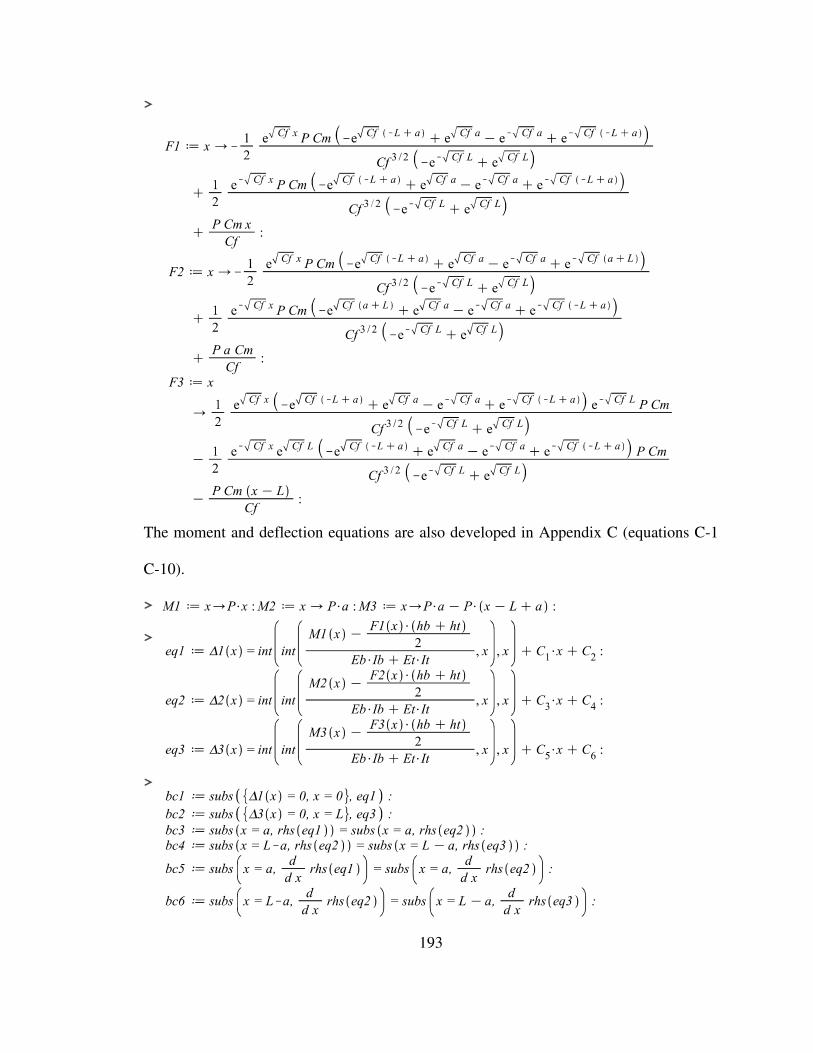
193
>
The moment and deflection equations are also developed in Appendix C (equations C-1
C-10).
>
>
>

194
>
The stiffness constants are described in section 2 as equations (2-18) and (2-19). The
keys nearest the ends of any particular beam were cut from the same piece of material,
and likewise for the next keys in, and so on, such that stiffness per unit length is based on
half of the keys distributed over half of the length.
Constant Terms
>
The displacement of the beam at the point loads can be determined by evaluating any of
the above deflection equations at the point load. The results of the evaluation yield the
displacement in terms of the applied point loads P . The total applied load to the beam
from the hydraulic ram R is 2P .
>
RamDefl=-0.00011900P=8403 16806
P R=

195
The above solution is for the first keyed beam using white oak keys. Additional
iterations of the process were conducted using the appropriate inputs from Table 6-1.
The results of those analysis are included in Table H-1.
Table H-1 Interlayer slip model analysis results
Test Key Cf Cm Deflection Stiffness
(10-4
) (10-5
) in/lb (10-5
) lb/in
1 OAK 6.11 6.46 11.90 16806
2 OAK 5.87 5.90 10.40 19228
3 PSL 21.29 21.22 7.53 26558
4 PSK 20.03 20.18 6.97 28708
H.2 Analysis of Test Data from Prior Research
The process used to analyze the interlayer slip model for comparison to Kidwell’s
(1897) research is similar to that outlined in section H.1, with the exception that the beam
was subjected to a single point load at midspan, rather than a symmetrically placed pair
of point loads. The Maple 11 (Maple, 2007) code is included below.
Input Parameters >
Geometry Calculations >
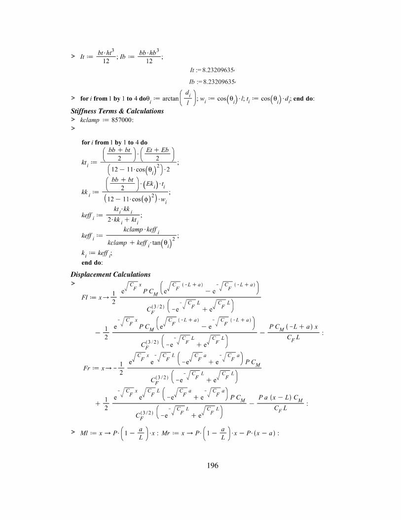
196
>
>
Stiffness Terms & Calculations > >
Displacement Calculations
>
>

197
>
>
>
Constant Terms
>
>
For a three-layer beam, a similar process, shown below, was used to calculate the
beam stiffness.
Input Parameters >

198
Geometry Calculations
>
>
Stiffness Terms & Calculations
>
>
Displacement Calculations
Rather than solve the set of governing differential equations for a beam with a
point load at midspan, the following equations, which were developed in Appendix B as
the closed form solution for a beam with any point, were used.

199
Constant Terms
>
>

200
Appendix I – Stress Calculations
The following is Maple 11 (Maple, 2007) source code for determining the stress
in the extreme fiber of a keyed beam. The inputs can be found in Table 6-1.
Input Parameters
>
Geometry Calculations >
>
>
Stiffness Terms & Calculations
>
>

201
Force & Moment Equations
>
>
Constants
>
>
Stress Calculations
>
The maximum stress occurs at the extreme fiber of a beam, either in the top or
bottom layer of a symmetric beam. Based on the sign convention used in developing the
interlayer stiffness model (see Figure 2-3), the distance to the extreme fiber on the top
layer of a two ply beam is 2T
h− . As the maximum stress on the top fiber is in
compression, the calculated stress is negative.
>