design and development of low-cost, high-temperature solar collectors for mass production ·...
TRANSCRIPT

Publ ic Interest Energy Research (P IER) Program FINAL PROJECT REPORT
DESIGN AND DEVELOPMENT OF LOW‐COST, HIGH‐TEMPERATURE SOLAR COLLECTORS FOR MASS PRODUCTION
MAY 2012CEC ‐500 ‐2012 ‐050
Prepared for: California Energy Commission Prepared by: The Regents of the University of California

Prepared by: Primary Author(s): Roland Winston University of California, Merced Merced, CA 95243 Contract Number: 500-05-021 Prepared for: California Energy Commission Michael Lozano Contract Manager Virginia Lew Office Manager Energy Efficiency Research Office Laurie ten Hope Deputy Director RESEARCH AND DEVELOPMENT DIVISION Robert P. Oglesby Executive Director
DISCLAIMER This report was prepared as the result of work sponsored by the California Energy Commission. It does not necessarily represent the views of the Energy Commission, its employees or the State of California. The Energy Commission, the State of California, its employees, contractors and subcontractors make no warrant, express or implied, and assume no legal liability for the information in this report; nor does any party represent that the uses of this information will not infringe upon privately owned rights. This report has not been approved or disapproved by the California Energy Commission nor has the California Energy Commission passed upon the accuracy or adequacy of the information in this report.

i
Acknowledgements
This work was supported by the California Energy Commission’s Public Interest Energy Research Program, Sol Focus, and the United Technologies Research Center). Authors acknowledge the guidance and assistance given by Heater Poiry, Steve Horne, Gary Conley, Randy Gee, Mary‐Jane Hale, and Guenter Fischer of Sol Focus Project team members included: Alfonso Tovar, Jesus Cisneros, Kevin Balkoski, Alexander Ritschel, Gerardo Diaz, Roland Winston‐ University of California, Merced and Randy Gee, Mary‐Jane Hale and Guenter Fischer of Sol Focus. Please site this report as follows: Winston, R. 2011. Design and Development of Low‐Cost, High‐Temperature Solar Collectors for
Mass Production. California Energy Commission Public Interest Energy Research Program Report: CEC‐500‐2012‐050.

ii
Preface
The Public Interest Energy Research (PIER) Program supports public interest energy research and development that will help improve the quality of life in California by bringing environmentally safe, affordable, and reliable energy services and products to the marketplace.
The PIER Program, managed by the California Energy Commission (Energy Commission), conducts public interest research, development, and demonstration (RD&D) projects to benefit California.
The PIER Program strives to conduct the most promising public interest energy research by partnering with RD&D entities, including individuals, businesses, utilities, and public or private research institutions.
PIER funding efforts are focused on the following RD&D program areas:
• Buildings End‐Use Energy Efficiency
• Energy Innovations Small Grants
• Energy Related Environmental Research
• Energy Systems Integration
• Environmentally Preferred Advanced Generation
• Industrial/Agricultural/Water End Use Energy Efficiency
• Renewable Energy Technologies
• Transportation
Design and Development of Low-Cost, High-Temperature Solar Collector For Mass Production is the final report for the project (Contract Number 500-05-021) conducted by the staff of the University of California Merced. The information from this project contributes to PIER’s Industrial/Agricultural/Water End‐Use Energy Efficiency and Renewable Energy Programs.
For more information about the PIER Program, please visit the Energy Commission’s website at www.energy.ca.gov/pier or contact the Energy Commission at 916-327-1551.

iii
Table of Contents
Acknowledgements ....................................................................................................................... i Preface ............................................................................................................................................ ii Table of Contents ........................................................................................................................ iii List of Tables ................................................................................................................................ ix Executive Summary ...................................................................................................................... 1 1.0 Introduction ........................................................................................................................ 8 2.0 Project Outcomes.............................................................................................................. 10 2.1. Task 2.0 ................................................................................................................... 10
2.1.1. Introduction ................................................................................................... 10 2.1.2. Applications .................................................................................................. 10
2.2. Task 3.0 ................................................................................................................... 26 2.2.1. Technical System Architectures for Application of Solar Heat .............. 26 2.2.2. Safety Considerations for XCPC Applications ...................................... 53
2.3. Task 4.0 ................................................................................................................... 55 2.4. Task 5 ...................................................................................................................... 66 2.5. Task 6 ...................................................................................................................... 95 2.6. Task 7 .................................................................................................................... 110 2.7. Task 8 .................................................................................................................... 121 2.8. Task 9 .................................................................................................................... 123 2.9. Task 10 .................................................................................................................. 144 2.10. Task 11 .................................................................................................................. 155 2.11. Task 12 .................................................................................................................. 163 2.12. Task 13 .................................................................................................................. 169 2.13. Task 14 .................................................................................................................. 170 2.14. Task 15 .................................................................................................................. 171 2.15. Task 16 .................................................................................................................. 179
2.15.1. Tested Collectors ......................................................................................... 179 2.15.2. Test Protocol ................................................................................................ 179 2.15.3. Description of Test Loop ........................................................................... 181 2.15.4. Instrumentation .......................................................................................... 183 2.15.5. Test Results of “Metal absorber with glass‐to‐metal seal – North‐South orientation” ................................................................................................................... 183 2.15.6. Test Results of “Metal absorber with glass‐to‐metal seal – East‐West orientation” ................................................................................................................... 189 2.15.7. Discussion .................................................................................................... 193
2.16. Task 17 .................................................................................................................. 198 2.17. Task 18 .................................................................................................................. 201 2.18. Task 19 .................................................................................................................. 207
2.18.1. Tested Collectors ......................................................................................... 208 2.18.2. Collector Thermal Efficiency: Method 1 .................................................. 208 2.18.3. Collector Thermal Efficiency: Method 2 .................................................. 209

iv
2.18.4. Temperature dependence of collector efficiency ................................... 209 2.18.5. Description of Test Loop ........................................................................... 210 2.18.6. Instrumentation .......................................................................................... 212 2.18.7. Test Results of “U‐Tube with Alanod Reflectors in North‐South orientation” ................................................................................................................... 212 2.18.8. Test Results of “U‐Tube with Alanod Reflectors in East‐West orientation” 216 2.18.9. Test Results of “X‐Tube with Alanod Reflectors in East‐West orientation” 219 2.18.10. Test Results of “U‐Tube with Reflectech Reflectors in North‐South orientation” ................................................................................................................... 223 2.18.11. Test Results of “U‐Tube with Reflectech Reflectors in East‐West orientation” ................................................................................................................... 228 2.18.12. Summary of Results ................................................................................... 231 2.18.13. Discussion .................................................................................................... 232
3.0 Conclusions and Recommendations .......................................................................... 260
List of Figures Figure 1. An Early XCPC Prototype at UC Merced ....................................................................................... 2 Photo Credit: The Regents of the University of California ........................................................................... 2 Figure 2. The 10kW SolFocus Test Loop at NASA/Ames ............................................................................. 2 Photo credit: The Regents of the University of California ............................................................................ 2 Figure 3. The 10kW B2U Prototype at GTI ...................................................................................................... 3 Photo credit: The Regents of the University of California ............................................................................ 3 Figure 4. Parallel Reflectors with Evacuated Glass Tubes ............................................................................ 4 Photo credit: The Regents of the University of California ............................................................................ 4 Source: The Regents of the University of California ...................................................................................... 5 Figure 5. XCPC Thermal Efficiency at Various Temperatures ..................................................................... 6 Source: The Regents of the University of California ...................................................................................... 6 Figure 6. Evolution of absorption chiller technology over the years ......................................................... 11 Source: The Regents of the University of California .................................................................................... 11 Figure 7. Broadʹs Double‐Effect Absorption Chiller .................................................................................... 13 Source: The Regents of the University of California .................................................................................... 13 Source: The Regents of the University of California .................................................................................... 13 Figure 8. Schematic of a typical adsorption chiller configuration.............................................................. 15 Source: The Regents of the University of California .................................................................................... 15 Figure 9. Solid (a) and liquid (b) desiccant technologies2 ........................................................................... 16 Source: The Regents of the University of California .................................................................................... 16 Figure 10. Vapor compression Figure 11. Organic rankine cycle ................................................... 18 Figure 12. Vacuum distillation system10 ........................................................................................................ 22

v
Figure 13. Solar Thermal Driven Single Effect Chilling System ................................................................. 27 Source: The Regents of University of California .......................................................................................... 27 Figure 14. Carrier 16JB single effect LiBr absorption chiller ....................................................................... 28 Figure 15 Diagram of a solar thermal driven double effect absorption chiller: using hot oil ............... 29 Figure 16. DN and 16 DE double effect chiller made by Carrier ................................................................ 30 Figure 17. Diagram of a solar thermal driven double effect absorption chiller: using steam ................ 32 Figure 18. Diagram of a solar thermal driven triple effect absorption chiller .......................................... 34 Figure 19. Trane and York triple effect chillers ............................................................................................ 35 Figure 20. Diagram of a solar thermal driven combined heating and cooling ......................................... 37 Figure 21 Solar ORC conceptual sstem architecture .................................................................................... 39 Figure 22. UTC Power PureCycleTM product ............................................................................................... 39 Figure 23. System parasitic power for single effect chillers ........................................................................ 43 Figure 24. System reliability block diagram .................................................................................................. 44 . Figure 25. System parasitic power for double effect chillers .................................................................... 46 Figure 26. System Parasitic Electric Consumption Sensitivity at full load ............................................... 47 Figure 27. Reliability block diagram XCPC driven double effect chillers ................................................. 48 Figure 28. On board parasitics for chillers ......................................................................................................... 49 Figure 29. Reliability block diagram XCPC driven double effect chillers ................................................. 50 Figure 30. Reliability block diagram XCPC driven ORC ............................................................................ 52 Figure 32: Top view and cross section view of XCPC concept #1 (drawing is not to scale) ................... 64 Figure 36. Projected XCPC Efficiency v Temperature ................................................................................. 67 Figure 37. All‐glass dewars – direct flow and all‐glass dewar filled with thermal fluid ‐ indirect flow ............................................................................................................................................................................. 68 Figure 38. Variation of selective coating absorptance with incidence angle ............................................ 69 Figure 39. Shape of XCPC reflector for all‐glass dewars ............................................................................. 70 Figure 40. Incidence Angle Modifier (IAM) for 58mm OD dewars ........................................................... 70 Figure 41. Incidence Angle Modifier (IAM) for design using absorber with glass‐to‐metal seal .......... 71 Figure 42. Sketch of all‐glass dewar tube (cross‐section) ............................................................................ 72 Figure 43. Sketch of all‐glass dewar tube (side cross‐section) .................................................................... 73 Figure 44. Metal absorber with glass‐to‐metal seal ...................................................................................... 73 Figure 46 & 47. Transversal section and schematic of heat fluxes ............................................................. 78 Figure 48. Corning Pyrex 7740 Transmittance curve ................................................................................... 79 Figure 49. ............................................................................................................................................................ 79 Figure 50. Heat fluxes at glass interface ........................................................................................................ 80 Figure 51. Heat fluxes at absorber interface .................................................................................................. 81 Figure 52. Heat fluxes at absorber / heat exchanger .................................................................................... 81 Figure 53. Thermal Circuit ............................................................................................................................... 83 Figure 53. Output temperature of fluid when irradiation is kept constant and while fluid input temperature varies according to table 1 ........................................................................................................ 85

vi
Figure 54. Differences in Temperature: Absorber – Input and Output ‐ Input ........................................ 86 Figure 55. Output temperature of fluid when input temperature is kept constant at Tin=400 K ........... 87 Figure 56. Differences in Temperature: Absorber – Input and Output ‐ Input ........................................ 87 Figure 57. Output temperature of fluid when input temperature is kept constant at Tin=473 K ........... 88 Figure 58. Output temperature of fluid when input temperature is kept constant at Tin=473 K ........... 89 Figure 59. Differences in Temperature: Absorber – Input and Output – Input ....................................... 89 Fiure 60. Spectral reflectance of Alanod Reflective Surfaces ...................................................................... 96 Figure 61: Measuring radius Figure 62: Reflectivity measurements of Alanod .............................. 97 Figure 63. Corning Pyrez 7740 Transmittance .............................................................................................. 98 Figure 64. Perkin‐Elmer spectrophotometer Figure 65. Perkin‐Elmer spectrophotometer .......... 99 Figure 66. Borosilicate Glass Tube Transmittance ........................................................................................ 99 Figure 68. Expected absorptance of selective coating as a function of incidence angle .........................102 Figure 69: Measured absorptance of selective coating as a function of incidence angle .......................102 Figure 70. Beijing Eurocon Heat Pipe Geometry and Characteristics ......................................................105 Figure 71. Manifold and Heat Pipe Arrangement .......................................................................................109 Figure 72. Direct Flow All Glass Dewar .......................................................................................................111 Figure 73. Ray Traces over the Design Acceptance Angle .........................................................................112 Figure 74. Horizontal Dewar Reflector Dimensions ...................................................................................113 Figure 75. Direct Flow Dewar Efficiency ......................................................................................................114 Figure 76. Vertical Dewar Reflector Dimensions ........................................................................................115 Figure 77. Indirect Flow Dewar .....................................................................................................................116 Figure 78. Expected Performance for Indirect Flow Dewar .......................................................................117 Figure 79. Metal Absorber Tube (Counter Flow) ........................................................................................118 Figure 80. Horizontal Metal Absorber Tube Reflector Dimensions .........................................................119 Figure 81 Performance predictions for three types of selective absorbers ...............................................120 Figure 82. Various collector efficiency equation coefficients .....................................................................121 Figure 83 Solar thermal energy output (assuming 50% efficiency) for a 991 m2 collector for a two day period June 2‐3 .................................................................................................................................................124 Figure 84. DOE‐2 output for four building types in Los Angeles .............................................................125 Figure 85. Absorption chiller COP as a function of the cooling water inlet temperature .....................126 Figure 86. Los Angeles retail store cooling load and solar heat profiles ..................................................127 Figure 87. Typical 48‐hour solar, cooling and electricity profiles of Los Angeles 120 ft2 retail ............128 Figure 88. Annual profile of cooling generation compared with the cooling demand ..........................128 Figure 89. A 3‐day profile of cooling generation compared with the cooling demand .........................129 Figure 90. Solar cooling ratio for the four buildings in the four cities. .....................................................129 Figure 91. Solar utilization ratio for the four buildings in the four cities. ...............................................130 Figure 92. Solar cooling capacity statistics ...................................................................................................130 Figure 93. Solar cooling capacity statistics ...................................................................................................131 Figure 94. Payback of the solar cooling system in Los Angeles ................................................................132

vii
Figure 95. Diagram of solar driven ORC ......................................................................................................133 Figure 96. Los Angeles ORC power generation and solar heat profiles ..................................................134 Figure 97. Typical 48‐hour solar heat and electricity generation profiles in Los Angeles .....................135 Figure 98. Total solar heat and power generation in four cities ................................................................135 Figure 99. ORC operation statistics ...............................................................................................................136 Figure 100. Solar driven ORC electricity savings ........................................................................................137 Figure 101. XCPC driven ORC payback as a function of ORC and solar collector costs .......................137 Figure 102. Payback of solar driven cooling system at different cities .....................................................138 Figure 103. Payback of solar driven cooling system with different chiller capacity ..............................139 Figure 104. Horizontal Glass to Metal Tube Efficiency ..............................................................................146 Figure 105. Horizontal Dewar Efficiency .....................................................................................................147 Figure107. Transmittance by Wavelength ....................................................................................................148 Figure 108. Metal Absorber Collector with AR ...........................................................................................149 Figure 109. Direct Flow Dewar with AR ......................................................................................................149 Figure 110. Spectral Reflectance.....................................................................................................................150 Figure 111. Metal Absorber with Reflectec ..................................................................................................151 Figure 112. Direct Flow with Reflectec .........................................................................................................151 Figure 113. Metal Absorber Design ...............................................................................................................152 Figure 114. Metal Absorber Thickness ..........................................................................................................153 Figure 115 Metal Absorber with AR and Reflectec .....................................................................................154 Figure 116. Direct Flow Tube with AR and Reflectec .................................................................................155 Figure 117. All glass dewar: direct flow Figure 118. Metal absorber with glass‐to‐metal seal .....157 Figure 119. Direct Flow Dewar ......................................................................................................................158 Figure 120. Metal Absorber ............................................................................................................................159 Figure 121. Annular Performance in a Diffused Environment ..................................................................160 Figure 122. Annular Performance in a Direct Solar Environment ............................................................160 Figure 123. Schematic of XCPC Design ........................................................................................................164 Figure 124. Cross section of absorber tube ...................................................................................................164 Figure 125. Evacuated glass tube with metal absorber (all units in mm) ................................................166 Figure 126. Manifold for North‐South orientation [all units in mm] ........................................................167 Figure 126b: Manifold for East‐West orientation [all units in mm] ..........................................................167 Figure 127b. Cross section of reflector for East‐West orientation .............................................................168 Figure 128. End view (upper drawing) and length view (three lower drawings) of frame for XCPC system in North‐South orientation ................................................................................................................169 Figure 129. Expected Optical Efficiency and Incidence Angle Modifier for East‐West orientation .....170 Figure 130. Expected thermal efficiency of XCPC .......................................................................................171 Figure 131. Schematic of Test Facility ...........................................................................................................173 Figure 132. Collector time constant ...............................................................................................................175 Figure 133. Example of a collector efficiency vs. temperature curve ........................................................178

viii
Figure 134. Schematic of Test Facility ...........................................................................................................182 Figure 135. North‐South Counterflow with Alanod Effective Reduced Efficiency Curve ....................185 Figure 136. North‐South Counterflow with Alanod Effective Standardized Efficiency Curve ............185 Figure137. North‐South Counterflow with Alanod Direct Reduced Efficiency Curve .........................186 Figure138. North‐South Counterflow with Alanod Direct Standardized Efficiency Curve .................187 Figure 139. North‐South Counterflow with Alanod: IAM Chart ..............................................................188 Figure 140. North‐South Counterflow Time Constant Plot .......................................................................189 Figure 141. East‐West Counterflow with Alanod Effective Reduced Efficiency Curve ........................191 Figure 142. East‐West Counterflow with Alanod Effective Standardized Efficiency Curve ................191 Figure 143. East‐West Counterflow with Alanod Direct Reduced Efficiency Curve .............................192 Figure 144. East‐West Counterflow with Alanod Direct Standardized Efficiency Curve .....................192 Figure 145. North‐South Counterflow with Alanod: Measured vs. Model .............................................193 Figure 146 East‐West Counterflow with Alanod: Measured vs. Model ...................................................195 Figure 147. Counterflow Efficiencies: North‐South vs. East‐West ............................................................196 Figure 148. Shows the comparison between expectations from modeling with achieved test results. ............................................................................................................................................................................199 Figure 149. Comparison of measured and modeled collector efficiency .................................................199 Figure150. Schematic of absorber tube used in tested XCPC ....................................................................200 Figure 151. Schematic of Test Facility ...........................................................................................................202 Figure 152. Collector time constant ...............................................................................................................204 Figure 153. Example of a collector efficiency vs. temperature curve ........................................................207 Figure 154. Schematic of Test Facility ...........................................................................................................211 Figure 155. North‐South U‐Tube with Alanod Effective Reduced Efficiency Curve .............................214 Figure 156. North‐South U‐Tube with Alanod Effective Standardized Efficiency Curve .....................214 Figure 157. North‐South U‐Tube with Alanod Direct Reduced Efficiency Curve .................................215 Figure 158. North‐South U‐Tube with Alanod Direct Standardized Efficiency Curve .........................215 Figure 159. East‐West U‐Tube with Alanod Effective Reduced Efficiency Curve ..................................217 Figure 160. East‐West U‐Tube with Alanod Effective Standardized Efficiency Curve .........................218 Figure 161. East‐West U‐Tube with Alanod Direct Reduced Efficiency Curve ......................................218 Figure 162. East‐West U‐Tube with Alanod Direct Standardized Efficiency Curve ..............................219 Figure 163. East‐West X‐Tube with Alanod Effective Reduced Efficiency Curve ..................................221 Figure 164 East‐West X‐Tube with Alanod Effective Standardized Efficiency Curve ...........................221 Figure 165. East‐West X‐Tube with Alanod Direct Reduced Efficiency Curve .......................................222 Figure 166. East‐West X‐Tube with Alanod Direct Standardized Efficiency Curve ..............................222 Figure 167. North‐South U‐Tube with Reflectech Effective Reduced Efficiency Curve ........................224 Figure 168 North‐South U‐Tube with Reflectech Effective Standardized Efficiency Curve .................225 Figure 169. North‐South U‐Tube with Reflectech Direct Reduced Efficiency Curve .............................225 Figure 170. North‐South U‐Tube with Reflectech Direct Standardized Efficiency Curve .....................226 Figure 171. North‐South U‐Tube with Reflectech stagnation test results ................................................227

ix
Figure 172. East‐West U‐Tube with Reflectech Effective Reduced Efficiency Curve .............................229 Figure 173 East‐West U‐Tube with Reflectech Effective Standardized Efficiency Curve ......................229 Figure 175. East‐West U‐Tube with Reflectech Direct Reduced Efficiency Curve .................................230 Figure 175 East‐West U‐Tube with Reflectech Direct Standardized Efficiency Curve ..........................230 Figure 176. East‐West U‐Tube with Reflectech: IAM Chart .......................................................................231 Figure 177. North‐South Collector Efficiency (Effective) ...........................................................................233 Figure 178. North‐South Collector Efficiency (DNI) ...................................................................................233 Figure 179. East‐West Collector Efficiency (Effective) ................................................................................235 Figure 180. East‐West Collector Efficiency (DNI) .......................................................................................235 Figure 181 U‐Tube Collector Efficiency (Effective) .....................................................................................236 Figure 182. East‐West Collector Efficiency (DNI) .......................................................................................237 Figure 183 Collector Efficiency (Effective) ...................................................................................................238 Figure 184. Collector Efficiency (DNI) ..........................................................................................................239
List of Tables
Table 1. Comparison of the XCPC System to Other Solar Thermal Systems ....................... 4 Table 2. Absorption Chillers, Generator Temperatures and COPs ...................................... 13 Table 3. Decision matrix for technology down selection ....................................................... 25 Table 4. Major design specifications for solar thermal driven single effect absorption chillers ....................................................................................................................................................... 27 Table 5. Major design specifications for oil driven solar thermal double effect absorption chillers ........................................................................................................................................... 30 Table 6. Major design specifications for oil driven solar thermal double effect absorption chillers ........................................................................................................................................... 33 Table 7. Major design specifications for oil driven solar thermal triple effect absorption chillers ........................................................................................................................................... 35 Table 8. Heating mode design specifications for an oil driven solar chilling/heating system ....................................................................................................................................................... 37 Table 9. Major design specifications for XCPC driven ORC cycle ....................................... 40 Table 10. Equipment cost estimates (less collector, storage tank and front end collector to tank piping) .................................................................................................................................. 53 Table 11. Comparison of Features ............................................................................................ 64 Table 12. Variation of output temperature of fluid when irradiation is kept constant at Gc = 326.7 W ......................................................................................................................................... 85 Table 13. Variation of output temperature of fluid when the input temperature is kept constant at Tin=400 K ................................................................................................................... 86 Table 14. Variation of output temperature of fluid when the input temperature is kept constant at Tin=473 K ................................................................................................................... 88

x
Table 15. Heat Pipe Heat Transport Limitations .................................................................. 106 Table 16. Estimated Heat Transport Limits ........................................................................... 108 Table 17. Condenser Side Heat Transfer Estimates .............................................................. 110 Table 18. Cost comparison of XCPC design concepts in high volume production (10,000 tubes) ........................................................................................................................................... 123 Table 19. System specifications for solar cooling system .................................................... 127 Table 20. Detailed analysis results for 120k ft2 retail store with solar cooling ................. 131 Table 21. System specifications for solar power generation system with ORC ............... 134 Table 22. Detailed analysis results with solar ORC .............................................................. 136 Table 23. Modeling of solar driven cooling for a 80k sq ft supermarket ........................... 141 Table 24. Modeling of solar driven cooling for a 120k sq ft retail store ............................ 142 Table 25. Modeling of solar driven cooling for a 270k sq ft hospital ................................. 142 Table 26. Modeling of solar driven cooling for a 270k sq ft hotel ...................................... 143 Table 27. Selective Foil Properties .......................................................................................... 145 Table 28. Cermet Properties ..................................................................................................... 145 Table 29. All Glass Dewar Advanced Cermet Coatings ...................................................... 146 Table 30. Component Improvement Summary .................................................................... 155 Table 31. Cost Comparison of XCPX Design Concepts in High Volume Production (10,000 tubes) ........................................................................................................................................... 161 Table 32. Down‐Select Matrix .................................................................................................. 163 Table 33. Summary expectations table ................................................................................... 171 Table 34. Collector Description of North‐South Counterflow with Alanod Collector .... 183 Table 35. Performance Characteristics of North‐South Counterflow with Alanod Collector ..................................................................................................................................................... 184 Table 36. Description of East‐West Counterflow with Alanod Collector ......................... 189 Table 37. Performance Characteristics of East‐West Counterflow with Alanod Collector190 Table 38. Comparison of the North‐South and East‐West Counterflow with Alanod collectors ..................................................................................................................................... 195 Table 39. Collector Description of North‐South U‐Tube with Alanod Collector ............. 212 Table 40. Performance Characteristics of North‐South U‐Tube with Alanod Collector . 213 Table 41. Description of East‐West U‐Tube with Alanod Collector .................................. 216 Table 42. Performance Characteristics of East‐West U‐Tube with Alanod Collector ..... 217 Table 43. Description of East‐West Counterflow with Alanod Collector ......................... 219 Table 44. Performance Characteristics of East‐West X‐Tube with Alanod Collector ...... 220 Table 45. Description of North‐South U‐Tube with Reflectech Collector ......................... 223 Table 46. Performance Characteristics of North‐South U‐Tube with Reflectech Collector224 Table 47. Stagnation test conditions for North‐South U‐Tube with Reflectech ............... 226

xi
Table 48. Description of East‐West U‐Tube with Reflectech Collector .............................. 228 Table 49. Performance Characteristics of East‐West U‐Tube with Reflectech Collector . 228 Table 50. Performance Summary of All Collectors Based on Effective Irradiation ......... 232 Table 51. Performance Summary of All Collectors Based on Direct Normal Irradiation232
Abstract This report describes the design and development a of low‐cost, high‐temperature solar thermal collector system for mass production with SolFocus, Inc. The external compound parabolic concentrator can be readily manufactured at a cost of $15 to $18 per square foot, and has an efficiency of 50 percent at a temperature of 400°F. During this project, a total of seven different external compound parabolic concentrator configurations were created and tested at the University of California, Merced. After improving the reflector technology and incorporating a new evacuated thermal absorber design, a prototype was constructed and tested. After further improvements and adjustments, a 10 kilowatt prototype was manufactured and tested by SolFocus at the NASA Ames Research Center in California. This prototype has been in operation since the spring of 2008. The project demonstrates a significant advance in solar thermal technology, with potential practical applications in the areas of solar heating, cooling, power generation, and desalination. External compound parabolic concentrator based systems could potentially replace natural gas driven systems, leading to a more conservative use of natural resources and a reduction in atmospheric pollutants including methane and carbon dioxide. As a result of this research, a new startup company, B2U Solar, was launched from SolFocus to commercialize the external compound parabolic concentrator technology. B2U Solar is developing applications in three areas with immediate potential, including: heating ventilation, and air conditioning, which employs double‐effect absorption cooling; industrial/commercial boiler or oil heater augmentation; and process heat. Keywords: Solar thermal collector, external compound parabolic concentrator XCPC, reflector, solar heating, cooling, power generation, desalination, atmospheric pollutants, B2U, HVAC

1
Executive Summary
Introduction Commercial solar thermal collectors at a distributed scale are predominantly flat plates that do not have the high temperature capability to provide process heat, power double effect absorption chillers, or produce electric power at high temperatures. A more cost effective solar thermal collector capable of producing heat at a temperature of approximately 400°F is needed for industries. The discovery and development of non‐imaging optics has enabled non‐tracking (fixed) concentrating solar collectors generating heat up to 600°F. In March 2002, Bergquam Energy Systems completed a project to design and optimize solar absorption chillers. This project, funded by Public Interest Energy Research program Renewables Program (contract number 500‐02‐035), was the first demonstration worldwide showing that a double effect absorption chiller can be powered by a solar thermal system, based on non‐imaging optics for the concentration of sunlight. Several overseas companies overseas took up this technology concept and developed similar products to be commercialized. However, most of these products are, in most cases, not cost‐competitive and not or geared to California’s climate requirements. This report describes the design and development of a of low‐cost, high‐temperature solar thermal collector system for mass production. Working with corporate participants, SolFocus and United Technologies Research Center, the research team at the University of California, Merced has developed an innovative non‐tracking system, consisting of a series of stationary evacuated solar thermal absorbers paired with external non‐imaging reflectors. Called an external compound parabolic concentrator, this system is able to operate with a solar thermal efficiency of 50% at a temperature of 400°F. The external compound parabolic concentrator can be readily manufactured at a cost of $15 ‐ $18 per square foot. During the course of this project, a total of seven different external compound parabolic concentrator configurations were tested, and an initial external compound parabolic concentrator prototype was created and tested at UC Merced (Figure 1). After improving the reflector technology and incorporating a new evacuated thermal absorber design, an improved prototype was constructed and tested. The East‐West collector with U‐Tubes and Reflectech reflectors performed the best out of our the tests, with roughly 47 percent efficiency at 200°C. After further improvements and adjustments, a 10 kW prototype was manufactured by SolFocus and tested at the NASA/Ames facility (Figure 2). This prototype has been in operation since the spring of 2008.

2
Figure 1. An Early XCPC Prototype at UC Merced Photo Credit: The Regents of the University of California
Figure 2. The 10kW SolFocus Test Loop at NASA/Ames Photo credit: The Regents of the University of California

3
The external compound parabolic concentrator can replace natural gas used for heat and space cooling with solar energy, leading to a more cost effective use of natural resources and decreased air emissions. Given that conventional flat plate collectors, and even the Winston‐Series Compound Parabolic Collector manufactured by Solargenix Energy, cannot operate with a positive efficiency at temperatures above 250°F, this project represents a major advance in practical solar heating, cooling and power generation. The success of this project has also stimulated the creation of a new company called B2U Solar. B2U Solar was recently spun out of SolFocus to commercialize the external compound parabolic concentrator technology. The company is already focusing its commercial efforts on immediate high potential areas, including: heating, ventilating, and cooling employing double‐effect absorption cooling; industrial/commercial boiler or oil heater augmentation; and process heat. A new prototype has been manufactured and installed by B2U at the Gas Technology Institute (GTI) in Chicago.
Figure 3. The 10kW B2U Prototype at GTI Photo credit: The Regents of the University of California Currently, UC Merced researchers are collaborating with industry on another high impact area for this technology. Evaluations are under way that could lead a new UC Merced research partnership focused on harnessing solar thermal energy for water desalination projects in California’s Central Valley and beyond. Technical Description

4
The external compound parabolic concentrator consists of a series of stationary evacuated solar thermal absorbers paired with external non‐imaging reflectors. The design consists of a set of parallel cylindrical absorbers, each of them placed in the center of an evacuated glass tube. Each absorber is thermally connected to a manifold using a U tube. Each glass tube is surrounded by a non‐imaging reflector made of Alanod aluminum. The basic design is shown in Figures 4.
Figure 4. Parallel Reflectors with Evacuated Glass Tubes Photo credit: The Regents of the University of California The advantage of using integrated heat pipes for the external compound parabolic concentrator is that the connection does not require plumbing since there is no exchange of fluid. This simplifies the installation, facilitates tube replacement and enhances the reliability. The external compound parabolic concentrator design allows for low‐cost mass production, because all components are currently mass produced and available at very low prices. When compared to existing system designs (see Table 1), the external compound parabolic concentrator system represents a major advance in the field of low‐cost high temperature solar thermal collectors Table 1. Comparison of the external compound parabolic concentrator system to other solar thermal systems
Technological concept Pros Cons
Flat plate collector Stationary Limited to temperatures well below 200°F
Parabolic Trough Can operate up to 600°F Tracking required

5
Technological concept Pros Cons
Integrated Compound Parabolic Concentrator (ICPC)
- No tracking required - Can operate up to
500°F
Expensive
External Compound Parabolic Concentrator (XCPC) [our approach]
- No tracking required - Amenable to low cost
mass production ($15 - $18 psf)
Limited to temperatures up to 450°F
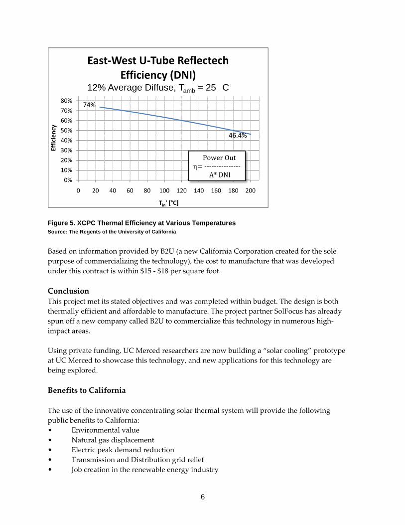
Source: The Regents of the University of California Project Objective and Outcome UC Merced’s objective for this project was to develop and demonstrate a new concentrating solar thermal collector system that is able to operate with a system efficiency of at least 50 percent at a temperature of 400°F, and to reduce the cost of a 400°F‐capable distributed‐scale solar thermal collector systems by 50 percent from the current $30 per square foot to $15 per square foot. Working with corporate participants SolFocus and United Technologies Research Center, the research team at the University of California, Merced has developed an innovative non‐tracking system consisting of a series of stationary evacuated solar thermal absorbers paired with external non‐imaging reflectors. Called an external compound parabolic concentrator, this system is able to operate at or near a solar thermal efficiency of 50% at a temperature of 400°F (see Figure 5).
6
Figure 5. XCPC Thermal Efficiency at Various Temperatures Source: The Regents of the University of California Based on information provided by B2U (a new California Corporation created for the sole purpose of commercializing the technology), the cost to manufacture that was developed under this contract is within $15 ‐ $18 per square foot. Conclusion This project met its stated objectives and was completed within budget. The design is both thermally efficient and affordable to manufacture. The project partner SolFocus has already spun off a new company called B2U to commercialize this technology in numerous high‐impact areas. Using private funding, UC Merced researchers are now building a “solar cooling” prototype at UC Merced to showcase this technology, and new applications for this technology are being explored. Benefits to California The use of the innovative concentrating solar thermal system will provide the following public benefits to California: • Environmental value • Natural gas displacement • Electric peak demand reduction • Transmission and Distribution grid relief • Job creation in the renewable energy industry
0%
10%
20%
30%
40%
50%
60%
70%
80%
0 20 40 60 80 100 120 140 160 180 200
Efficiency
Tin' [°C]
East‐West U‐Tube Reflectech Efficiency (DNI)
12% Average Diffuse, Tamb = 25 C
Power Outη ‐‐‐‐‐‐‐‐‐‐‐‐‐‐‐
A* DNI
46.4%
74%

7
8
1.0 Introduction This project demonstrates the effects of the design and configuration change in an evacuated tube based solar thermal collector utilizing non-tracking compound parabolic concentrators. High temperature operation (400° F) was achieved with acceptable optical and overall efficiencies. Design enhancements in the evacuated tube assemblies focused primarily on the flow paths to optimize heat transfer and flow rates. Three designs were evaluated in east-west (horizontal) and north-south (vertical) configurations. Compound parabolic concentrators were designed with a wide acceptance angle to facilitate use without the need of a tracking mechanism. Alanod and Reflectech were used to line the concentrators. Each were evaluated separately to ascertain their respective impacts on optical and overall system performance. A 10 kW prototype system was built and evaluated by SolFocus, Inc. The system performed well; however, the optimum configuration was dependent on the desired operating temperature.

9

10
2.0 Project Outcomes
2.1. Task 2.0
2.1.1. Introduction This report summarizes the findings of a broad survey conducted by the United Technologies Research Center (UTRC) with the objective of identifying promising applications for the external compound parabolic concentrator (XCPC) solar heat collector technology being developed by UC Merced and SolFocus. The survey focused on identifying applications that could operate on waste or solar generated heat in the temperature range of 200° F to 500° F. This represents the potential upper and lower bounds for working fluid from the solar thermal collectors. The applications surveyed can be qualified into four broader categories:
a) Heat driven cooling/heating technology b) Heat driven electric power generation technology c) Heat driven water treatment technology d) Heat driven industrial processes
The identified applications in each of these categories were evaluated based on the following evaluation criteria:
1) Technical feasibility and viability – Related to the ease with which the application could be integrated with the XCPC collector and the overall effectiveness of the application
2) Economic competitiveness – Related to the envisioned cost of the integrated system against other alternatives
3) Market potential – Related to the target markets that might be serviced by the envisioned product and its relative competitiveness in those markets
4) Time to commercialization – Related to the time it would take to commercialize the integrated system
5) Other considerations – Related to the institutional and legal barriers that might hinder commercialization of the envisioned system
2.1.2. Applications The applications were ranked based on qualitative assessments in each of the evaluation criteria. Based on these assessments two technologies were selected for further study (see Task 3 reports). These include:

11
a) Solar driven cooling/heating using absorption chillers (single, double and triple effect)
b) Solar driven organic Rankine cycle (ORC) for electrical power generation Heat driven cooling/heating technologies Thermal energy captured in the working fluid that circulates through the XCPC collectors can be used in conjunction with various thermally activated cooling technologies (TAT)1 to produce chilled water that can be used in cooling and refrigeration applications. Alternatively, the thermal energy can be used to remove humidity from the air which is desirable in comfort and food storage applications. There are three major types of TAT cooling technologies that could work with the XCPC collectors. These include: absorption chillers, adsorption chillers and desiccant systems.
Some of the absorption chillers offered in the market today can operate in both heating and cooling mode. It may be possible to recover some additional heat (for space heating) from the XCPC working fluid that exits the chiller, but it is likely that such an alteration might adversely impact the collector efficiency. Absorption chillers technology basics
The Department of Energy – Distributed Energy Program, has a very detailed description on the technology basics of absorption chillers. Figure 6 below shows a timeline for the evolution of absorption chiller technology over the years.
Figure 6. Evolution of absorption chiller technology over the years Source: The Regents of the University of California Briefly, the absorption chiller uses a thermal method for compressing the refrigerant vapor compared to the mechanical method (compressors) used in most electric vapor compression

12
(VC) chillers. The equipment typically uses a working fluid pair such as ammonia‐water or lithium bromide‐water and the amount of cooling provided can range from a few refrigerant tons for residential applications to more than one thousand tons for commercial applications. The ammonia‐water pair has been in limited usage for several years due to the toxicity issues associated with ammonia. In current lithium bromide – water based chillers, water is the refrigerant and aqueous lithium bromide is the absorbent. Water in vapor phase exiting the evaporator is absorbed by the lithium bromide solution in the absorber and this solution is pumped to the generator where heat is used to remove the water from the lithium bromide solution which is subsequently pumped back to the absorber. Several designs use natural gas or other fuel driven methods to provide heat to the generator. Thermal energy obtained from industrial waste heat sources, solar etc. could be used as an alternative method for heating the generator stage. This can provide added benefits of reduced emissions and minimize energy costs (less fuel consumed). The performance metric for cooling cycles is the coefficient of performance (COP) and enhancing the amount of water produced using the refrigerant vapor from a high stage generator can enhance performance of the absorption chiller. Absorption chillers are thereby offered as single effect, double effect and triple effect chillers with the key distinction among the three technologies being the number of generators used in the chiller and the temperatures at which they operate. Figure 7, shows a schematic of BROAD’s double effect absorption chiller where the heat is generated by burning natural gas.

13
Figure 7. Broad's Double-Effect Absorption Chiller Source: The Regents of the University of California
Table 2 ,summarizes the generator temperatures and associated COPs typical for the three types of absorption chiller technologies Table 2. Absorption Chillers, Generator Temperatures and COPs Chiller type Temperature range COP rangeSingle effect > 185 F 0.5‐0.75Double effect > 285 F 1.1‐1.4Triple effect > 350 F 1.5‐1.8Source: The Regents of the University of California Technology Evaluation Technical feasibility and viability Absorption chillers have been successfully demonstrated for several integrated applications with waste heat. Solar driven absorption chillers were demonstrated by

14
Carrier in the 1970s and additional demonstration work has been performed by Broad and other major heating, ventilating, and cooling (HVAC) companies as well. All the work done so far suggests a high degree of technical feasibility for a XCPC driven absorption chiller. Economic competitiveness Economic competitiveness for the integrated XCPC with the absorption chiller system largely depends upon the ability of the XCPC to hit cost targets of <$100/m2. In doing so, the operational expenditures for the system are comparable to absorption chillers operating on natural gas (~4 cents/kWh). Rising fuel costs further enhance the attractiveness of the absorption chiller option. Market potential Absorption chillers in the US market compete with electrically driven vapor compression chillers and cheap electricity prices have prevented their mass adoption in this market. The VC systems have COP’s in the range of: 3‐4. This implies that the higher the COP of the thermal activated technology (TAT) chiller, the greater the chance it has of capturing the market share, particularly when consumer electricity prices are on the rise especially in California. Time to commercialization Single and double effect chillers have been available in the commercial space for several years, and Kawasaki has recently introduced triple effect chillers in the Asian market. This implies that successful commercial development of the XCPC in two years could lead to integrated chiller product offerings within five years. Other considerations Potential legal and institutional barriers for an integrated XCPC‐chiller product will depend primarily on the type of working fluid used in the XCPC and the ability to safely install the collectors and transport this fluid to the chiller. Corrosion issues and refrigerant leaks are the main concerns for absorption chiller systems from a legal and institutional perspective and technology maturity coupled with market adoption dictates how these barriers are overcome. The chiller systems themselves are commercial products and there should be no major institutional barriers for single and double effect chillers. Triple effect chillers on the other hand might require additional qualification before they can penetrate the US market primarily because of the lower technology maturity of these systems. Adsorption chillers technology basics
Adsorption chillers3, 4 have been considered as alternatives for absorption chillers because of their lower operating temperatures and potential advantages such as no corrosion issues,

15
no hazardous leaks etc. (primarily associated with lithium bromide solutions in absorption chillers). A typical working pair in the adsorption chiller is water (refrigerant) and silica gel (adsorbent). In this system there are two adsorbent beds that alternate between a generation stage and an adsorption stage. The generation stage requires heat and this heat can be provided by various renewable and non‐renewable sources. The heat source temperatures for these systems can be in the 120° F to 200° F range (lower limit of the XCPC) and their COPs are usually lower than single effect absorption chillers (close to 0.6). Figure D, shows a schematic of an adsorption chiller cycle.
Figure 8. Schematic of a typical adsorption chiller configuration Source: The Regents of the University of California
Technology Evaluation
Technical feasibility and viability Adsorption chillers are present in the Japanese market today and HIJC USA Inc. in the United States is marketing a Japanese product. Integration of this device with the XCPC while feasible may not necessarily be the best use of the high quality heat that is obtained from the XCPC. Economic competitiveness Adsorption chillers at a COP of 0.6 could compete favorably with single effect chillers from

16
a cost and reliability perspective. Double effect machines with higher COPs (more cooling capacity per unit of thermal energy input) are economically more competitive than current adsorption chillers. Market potential Adsorption chillers could compete well as cooling technology offered in markets where low grade waste heat (<200 F) is readily available. The low COP of these devices makes their ability to displace vapor compression chillers even more difficult than double effect absorption chillers. Time to commercialization Adsorption chillers are available in the market today and while an XCPC integrated adsorption chiller could be commercialized, the current technology with its lower temperature of operation is not the ideal fit for the XCPC collector. Future generation adsorption chillers with higher COPs and higher temperature operations could be better fits; however, no such device is available commercially. Other considerations There seem to be no major legal or institutional barriers that might prevent the current water‐silica gel based adsorption chillers from entering the market. Attempts to improve the COP might require moving to refrigerants such as ammonia and this may introduce barriers primarily due to concerns about toxicity of the refrigerant.
Desiccant cooling technology basics
Desiccant cooling2 is a popular method for humidity control and the basic principle for this technology is the use of a sorbent material to remove moisture from an air stream. The sorbent material can be solid (silica gel, alumina etc.) or liquids (lithium chloride, glycol etc.). Thermal energy is used to regenerate the sorbent material and waste heat or solar could be one of the sources of this thermal energy. Several companies including Carrier, Munters, AIL Research etc. to name a few offer desiccant based humidity control products.
(a) (b) Figure 9. Solid (a) and liquid (b) desiccant technologies2
Source: The Regents of the University of California

17
Technology Evaluation
Technical feasibility and viability Most of the desiccant systems can operate with low quality waste heat (as low as 150° F) and while it is technically feasible to interface this with the XCPC, this particular application may not be the best use of the high quality thermal energy obtained from the collectors. Economic competitiveness The desiccant systems can be expensive products and the economic competitiveness of an integrated system will primarily depend on making the collector prices competitive with the current method used for regenerating the sorbent material. Since the quality of heat required to regenerate sorbent materials in desiccant systems is quite low, there are cheaper off the shelf low temperature thermal collectors that may be a better choice for an integrated solution. Market potential Market potential for desiccant based dehumidifiers was projected to be $300 M in North America in 20066. The market share for solar driven desiccant dehumidifiers is not significant and it is unclear if the XCPC would offer any benefit in terms of penetrating into this market. Time to commercialization Several desiccant cooling system products exist today and it is conceivable that any potential solar integrated desiccant product can be developed in a span of 1‐2 years. Other considerations Solid desiccant systems are the most prevalent in the market today; and, there are almost no legal or institutional barriers preventing the adoption of this technology. However, working fluid in the solar collector, and the need to pump corrosive fluids in liquid desiccant systems could be of concern from an institutional stand point. Heat driven electrical power generation Currently, one of the more popular methods for converting solar energy to electrical energy in the distributed power generation market is photovoltaic technology. Solar thermal based power generation cycles have been demonstrated for utility scale applications. Creating a distributed solar thermal electrical generation product that could compete by offering lower leveled cost of electricity than PV could provide a path to capture a share of the growing $11 B/yr solar electricity generation market. There are three types of distributed generation products that could be compatible with the XCPC. These include:
a) ORC based products b) Steam cycle based products c) Stirling cycle based products.

18
Organic Rankine Cycle based products technology basics The Organic Rankine Cycle (ORC), in simple terms, is a vapor compression cycle that is operated in reverse. Figures 10 and 11, are a schematic representation of an ORC compared to a traditional VC refrigeration cycle. The motor and the compressor used to compress the refrigerant are replaced by a turbine and a generator. The overall efficiency is sensitive to (among other factors) the type of refrigerant used in the system. The key interface between XCPC collector working fluid and the ORC would be the evaporator/boiler heat exchanger. This heat exchanger would have to be appropriately designed based on the working fluid that is finally selected for the collector. Companies such as ORMAT, UTC Power etc. currently offer ORC products that could be readily interfaced with the XCPC.
Figure 10. Vapor compression Figure 11. Organic rankine cycle Source: The Regents of University of California Source: The Regents of University of California Technology Evaluation
Technical feasibility and viability There are a couple of commercialized ORC products including the PureCycleTM from UTC Power that could use heat provided by XCPC collectors to produce power for distributed applications. The temperature from the XCPC is within the desired range required for operation of this product (demonstrated for temperatures as low as 200 oF). One of the important elements that may need to be redesigned for an integrated system is the supervisory control to enable seamless performance under transient solar insolation conditions. Economic competitiveness The PureCycleTM product in volume would cost in the neighborhood of $1/W and this coupled with low cost XCPC would offer customers a solar based electrical power generation solution that is about half the cost of conventional photovoltaic (PV) today. The key advantage of the integrated product is that the components that comprise the core power generating system exist as virtual commodities in volume production today.

19
Market potential A distributed solar‐ORC product would compete in the space occupied by conventional PV today. Initial markets would likely include big box retail stores, supermarkets etc. that are projected to be in the $4 B range by 2010 (based on projections from the PV industry). Time to commercialization The current PureCycleTM product can operate at temperatures up to 300 oF and the integrated product with an XCPC operating at this temperature could be offered within a five year time frame. There might be the possibility of altering refrigerants so that the cycle operates at higher temperatures and higher efficiencies. These systems might take well over five years to develop. Other considerations Currently there are no major legal or institutional barriers envisioned for an integrated product given that the ORC is a commercial offering. Changing regulations on refrigerant usage could become a major consideration especially when designs need to be improved from an efficiency standpoint. The system will require compliance with electrical codes and standards should it become a grid tied product.
Steam Cycle Based products Technology basics Steam cycles work on the operating principle of feeding high pressure steam into rotating turbomachinery that converts the mechanical energy to electrical energy using a motor. Utility scale solar thermal energy driven steam cycles8 have been demonstrated as part of the DOE‐Solar Energy Technologies Program (SETP). Recently Carrier9 has introduced a micro‐steam generator product that is targeted towards the distributed generation market and this product may be an ideal integration candidate if the XCPC heat is used to create high pressure, wet steam.
Technology evaluation
Technology feasibility and viability The technology in theory should be feasible and viable but there may be some redesign required for the generator during transient operation (periodic dip in solar insolation and/or working fluid flow rate temperatures). Efficiency would be low in this system because of the limitation on the maximum cycle temperature and the steam turbine would likely have to deal with the erosive effects of wet steam. Initial iterations of a product such as this might only be viable in places where there are existing high pressure steam lines where solar meets only part of the total steam requirements for the system. Economic competitiveness Economic competitiveness of an integrated system will depend upon lowering the XCPC costs such that the steam generated from these collectors costs less than the yearly costs of steam ($0.015/lb9) incurred by a system that is installed in a location with existing high
20
pressure steam lines. Market potential The ability of the integrated system to penetrate and capture solar power generation markets will depend upon being able to beat current levelized cost of electricity from PV systems. This market as mentioned earlier is in the billions of dollars regime and to ultimately be competitive in the absence of incentives and rebates, the cost of electricity for the system would have to be less than grid electric prices. Time to commercialization An integrated XCPC‐micro steam turbine product would probably require about five years or more (including time taken to commercialize the XCPC collectors) of development due to reasons mentioned in the feasibility assessment. Other considerations It is unlikely that a fully integrated system would have major legal or institutional barriers preventing adoption other than those related to leakage issues of the working fluid selected for the XCPC collector. Electrical codes and standards will apply if the system is grid connected. Steam systems in certain buildings might have significant code barriers and this is something that will need to be overcome to capture the broader market.
Stirling Cycle Based products
Technology basics The Stirling cycle has a fixed amount of working fluid and a piston (or pistons) in a sealed space. The piston(s) are moved by heating and cooling the sealed space and this movement produces rotational, mechanical motion that can be converted to electrical energy using a generator. The choice of the working fluid is therefore one of the critical elements in the selection of an appropriate Stirling engine. It needs to be environmentally benign and work at the temperatures supplied by the XCPC collector. Dish solar collector based Stirling engines have been a topic of Department of Energy (DOE) research for several years. Some of these require working temperatures as high as 700 oC and the primary benefit of operating at higher temperatures is higher efficiency. The moderate working temperature of the XCPC compared to the higher temperatures might result in a lower efficiency operation of the Stirling engine. Technology evaluation
Technology feasibility and viability It is technically feasible to demonstrate a Stirling engine integrated to an XCPC array. Although the Stirling cycle has a high theoretical efficiency because it is a close approximation of the Carnot cycle, the actual efficiency is quite low because of practical limits on the effectiveness of heat exchanger devices. The efficiency and performance of such a device is unknown and it is unclear if these would perform better than the dish Stirling systems offered today.

21
Economic competitiveness The system will have to be cheaper and operate at comparable efficiencies to be competitive with dish Stirling engines today. The system could compare favorably with an ORC but in this case it must meet a fairly low capital cost metric and it is unclear if some of the current Stirling systems could meet these cost metrics and stay competitive. Market potential The market potential in this case will also depend upon the ability of the system to offer competitive levelized cost of energy to the customer. Time to commercialization Stirling engine systems are commercially available from companies such as WhisperGen, Sun Power, Stirling Energy Systems etc. Time to commercialization of an integrated system will depend upon how the XCPC heat can be integrated to some of these engine systems and it is unclear at this point on how long this might take. Other considerations The institutional and legal barriers for an integrated system will depend upon the working fluid in the collector and the engine. Furthermore, electrical codes and standards for grid connected systems will also apply. Heat driven water treatment technology Water desalination and purification is important to several industrialized and developing nations. Water desalination requires removal of salt from various types of water sources including sea water, brackish water etc. with the objective of providing fresh water for every day consumer use. There are two main types of desalination technologies that are most prevalent today. The most common are various distillation processes that require high temperatures for operation. The second type is reverse osmosis which requires high pressures to drive pure water through a membrane separation process. Water purification focuses more on the removal of various particulate, organic and inorganic impurities from existing fresh water supplies or when attempting to implement water reclamation projects. Membrane technologies are popular methods for particulate removal. Other methods include adding some type of chemical such as chlorine, ozone etc., that can chemically react to remove certain organic compounds and/or biological organisms. Most of the water purification technologies do not require the high temperatures that can be generated by the XCPC for operation. Solar desalination methodology involves using a solar still that evaporates water from sea water and collects fresh water through condensation. The process has a very slow throughput which is why even in some of the parts of the world with good solar insolation, other methods of water desalination are used. The thermally driven methods of water purification derive their thermal energy through the burning of fossil fuel (mostly natural gas). Consequently, the biggest value for XCPC generated heat might be in some of the distillation technologies as a substitute for the thermal energy generated by fuel. Two specific technologies that could fit within this realm include: a) Vacuum distillation and b) Membrane distillation.

22
Vacuum Distillation technology basics
Vacuum distillation works on the principle that by lowering the pressure of a salt water solution, it is possible to evaporate the water off at low temperatures (as low as 100 oF)10. The method is commonly used in large scale co‐generation plants that produce electricity from natural gas and uses the waste heat from the process to distill sea water. A key tradeoff that occurs with the technology is that with lower quality waste heat, the vacuum pump may have to be designed to provide very low pressures and this may increase the electrical power consumed by the pump. Companies such as WasTech offer packaged vacuum distillation products for industrial use.
Figure 12. Vacuum distillation system10
Source: The Regents of University of California Technology evaluation
Technical feasibility and viability It should be technically feasible to use heat from the XCPC to drive a low temperature vacuum distillation process. The temperatures required are low enough that the process could even be driven by low temperature collectors today. It is possible that one of the reasons why a system such as this has not been implemented is due to the fact that these units operate in industrial processes where there should be other sources of low quality waste heat by negating the need for solar driven processes. Economic competitiveness It is unlikely that an XCPC driven vacuum distillation system would give any significant competitive advantage unless the power consumed by the vacuum pump is substantially reduced by adapting the system to operate at higher grade heat. In this case the realized cost savings due to lowered electricity consumption would have to be traded against the cost of utilizing XCPC heat. Market potential The integrated product if commercially and technically viable should have tremendous market potential because of growing demands for water desalination products both in California and worldwide. Time to commercialization

23
The integrated product could take between 5‐10 years to commercialize if an appropriate skilled vendor is identified in the field of water desalination to support the development project. Other considerations The legal and regulatory barriers for the integrated technology will be associated with demonstrating the quality of the water obtained from the process.
Membrane Distillation technology basics Membrane distillation operates using a temperature differential driving force that creates vapor pressure differentials between two sides of a membrane module. One side of the membrane circulates cool, clean water with heated brine solution flowing on the opposite side. The temperature differential between the solutions results in vapor being formed from the brine solution and transported across the membrane pores where it condenses to fresh water upon contacting the cold side. This technology has been demonstrated for temperatures up to 80 oC in university studies11 but there are no products available in the market place today that are based on membrane distillation. Technology evaluation
Technical feasibility and viability It is difficult to say if an integrated XCPC‐membrane distillation system can be successfully demonstrated primarily because it may be difficult to obtain a durable membrane that operates at the higher temperatures (>150 oC) provided by the collectors. Economic competitiveness The current technology if successfully commercialized could compete favorably with reverse osmosis and other distillation processes. Initial costs of these units however may be high to factor in recovery of research and development expense.
Market potential The product could compete well in the global water desalination market if the technology can be commercialized and it beats the more mature desalination product technologies in the market place today. Time to commercialization High temperature membranes will have to be developed so that the distillation process can operate at the thermal output provided by the XCPC. This requires technology development and it is conceivable that the system itself could take several years to develop. Other considerations The major institutional barrier to be considered is the fact that the integrated product would have to be qualified in terms of the quality of water provided by the systems. The barriers can be successfully overcome if appropriate testing protocols and standards are first developed for a standalone membrane distillation process.

24
Heat driven industrial processes The thermal energy from the XCPC can certainly be integrated into industrial processes that require supplemental heat to drive certain processes. One such application is in industrial drying processes. The large food production and processing industry in California uses enormous amounts of heat for cooking, packaging and cleaning and this could be another potential market for the heat collected by the XCPC. The complication with implementing the XCPC in these scenarios is that industrial processes tend to be highly integrated in terms of their thermal management schemes. These processes also often require continuous 24/7 or 16/5 supply of the heat. The value for the thermal energy from an economic perspective is consequently lower in these cases compared to building integrated power generation and/or cooling and heating applications. The generation of renewable solar fuels is an area that could offer a future application space for the XCPC. Several technology options in this area have been identified as critical areas of research by the DOE Office of Basic Energy Sciencies (BES)12. Advanced catalytic and biomemetic approaches that convert biological waste, carbon dioxide, water etc. to fuels, requiring process temperatures in the neighborhood of 250 oC could be a good fit with XCPC generated process heat. This report has avoided providing an evaluation of these options due to their low technology maturity. It is important to note however that if these breakthrough technologies are successfully commercialized, a whole new area could be opened up for applying XCPC derived solar thermal energy Ranking Technology options The five categories for technology evaluation were assigned the following weights based on preferred importance: a) Technology feasibility and viability (TF‐0.3), b) Economic competitiveness (EC‐0.2), c) Market potential (MP‐0.2), d) Time to commercialization (TC‐0.2) and e) Other considerations (OC‐0.1). The possible scores for each category used were in the range of 1‐3. The market potential in our assessment follows the order power generation > cooling/heating > water desalination. This is based on the fact that there are products for the first two applications that encompass the residential, commercial and industrial markets. Water desalination is primarily industrial and commercial with limited application in the residential space. Table 3 below presents the decision matrix used to guide high level system design efforts for Task 3 of the contract.

25
Table 3. Decision matrix for technology down selection
Application Technology
TF (0.3)
EC (0.2)
MP (0.2)
TC (0.2)
OC (0.1)
Total Score
Cooling/Heating Absorption 3 2.5 2.5 3 2.51 2.75 Adsorption 2.5 2 2.5 2.5 3 2.45 Desiccant 2 2 2.5 2.5 3 2.3
Power Generation
ORC 2.5 3 3 2.5 2.52 2.7 Steam cycle 2 3 3 2.5 2.5 2.55
Stirling Cycle 2 2 3 2.5 2.52 2.35
Water Desalination
Vacuum Distillation 2 2 2 2 2 2
Membrane Distillation 1.5 2.5 2 1.5 2 1.85
Source: The Regents of University of California Conclusions and recommendations Based on the assessment in this report it is recommended that an ideal near term focus for a future project would be XCPC integration with absorption cooling and ORC electrical power generation technologies. Next generation efforts could focus on integration with distributed steam (the micro‐steam turbine for example) and Stirling cycles. Finally, over the longer term, the XCPC integration with water desalination technologies is worth considering. It is also recommended that UC Merced partner with other universities and/or companies in the development of basic technology for the emerging area of solar fuels with a focus around processes that operate at < 250 o

26
2.2. Task 3.0 2.2.1. Technical System Architectures for Application of Solar Heat This report summarizes conceptual system architectures for the five potential applications for process heat from the XCPC that were identified from a broad survey that was conducted earlier (Task 2 report – “Report on Application Areas of Solar Heat”).
System configurations that are discussed in this report include:
XCPC driven single effect chilling
XCPC driven double effect chilling (b1: oil or b2: steam as hot working fluid)
XCPC driven triple effect chilling
XCPC driven combined chilling and heating
XCPC ORC
To compare different architectures, we assume the same chilling capacity of 120 refrigeration tons (RT) for all chillers, which is good for a mid‐size office building in a moderate hot climate such as Washington, D.C., in summer. The solar thermal capacity needed to drive the absorption chiller will match the cooling capacity. The technical specifications are provided are as generic as possible. Commercial data are referenced wherever appropriate to better illustrate the system working characteristics. Conceptual designs have been arrived at using simple high level engineering calculations that also provide details on the key operating parameters for the system. XCPC driven single effect chilling The diagram of a solar thermal driven single effect chilling system is shown in Figure 13 below.

27
Figure 13. Solar Thermal Driven Single Effect Chilling System
Source: The Regents of University of California In this system, water is pumped to the solar collector and then heated to a temperature below the boiling point. The heated water is sent to a hot water storage tank. Hot water leaving the storage tank enters into the generator of a single effect Lithium bromide (LiBr) absorption chiller. The absorption chiller produces chilled water through the evaporator to cool the desired space. A cooling tower is needed to serve as the heat sink for the system. Table 4. Major design specifications for solar thermal driven single effect absorption chillers Unit
Design Specifications Value (SI) (SI) RemarksSolar collector capacity 670 kW Water heating system efficiency 0.90 Assumed value
Assume water supply temperature Hot water temperature produced 92 C + 2C
Assume return water temperature Design incoming hot water temperature 78 C - 2C Pump flow rate 11.4 kg/s 181 GPM
Variable Hot water pump type speed Storage tank capacity 41 m^3 Assume 1 hour full load supply
Single Chiller type effect Chiller capacity 120 RT Assumed benchmark capacityChiller COP 0.7 A typical value
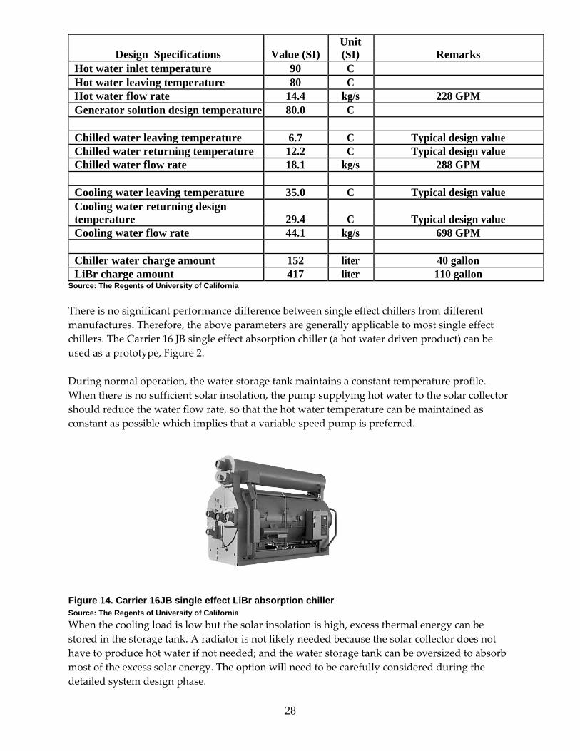
28
Unit Design Specifications Value (SI) (SI) Remarks
Hot water inlet temperature 90 C Hot water leaving temperature 80 C Hot water flow rate 14.4 kg/s 228 GPMGenerator solution design temperature 80.0 C
Chilled water leaving temperature 6.7 C Typical design valueChilled water returning temperature 12.2 C Typical design valueChilled water flow rate 18.1 kg/s 288 GPM
Cooling water leaving temperature 35.0 C Typical design valueCooling water returning design temperature 29.4 C Typical design valueCooling water flow rate 44.1 kg/s 698 GPM
Chiller water charge amount 152 liter 40 gallonLiBr charge amount 417 liter 110 gallon
Source: The Regents of University of California There is no significant performance difference between single effect chillers from different manufactures. Therefore, the above parameters are generally applicable to most single effect chillers. The Carrier 16 JB single effect absorption chiller (a hot water driven product) can be used as a prototype, Figure 2. During normal operation, the water storage tank maintains a constant temperature profile. When there is no sufficient solar insolation, the pump supplying hot water to the solar collector should reduce the water flow rate, so that the hot water temperature can be maintained as constant as possible which implies that a variable speed pump is preferred.
Figure 14. Carrier 16JB single effect LiBr absorption chiller Source: The Regents of University of California When the cooling load is low but the solar insolation is high, excess thermal energy can be stored in the storage tank. A radiator is not likely needed because the solar collector does not have to produce hot water if not needed; and the water storage tank can be oversized to absorb most of the excess solar energy. The option will need to be carefully considered during the detailed system design phase.

29
When there is high cooling demand but low solar energy, hot water in the storage tank is drained at a rate higher than the thermal energy produced in the collector. The average hot water temperature in the tank will decline. When the hot water temperature going to the chiller deviates within a few degrees, the absorption chiller cannot work properly and the building backup chillers, usually electrically driven vapor compression chillers, have to be used.
The advantage of single effect absorption chillers that they requires relatively low hot water temperature which means the water can be pumped at atmospheric pressure. The system is simple, commercially available, and the reliability is high. The major disadvantage is that the COP of the chiller is low and a larger solar collector is needed to provide the same amount of cooling load. Furthermore, since the quality of waste heat required for these chillers is lower than the temperature delivery capabilities projected for the XCPC, there may be a need to use the chiller as a bottoming cycle which works of the exhaust heat from a higher temperature component.
XCPC driven double effect chilling A double effect absorption chiller can be used when the heating fluid temperature is sufficiently higher than the solution temperature in the high pressure generator (HPG) of the chiller. The solution temperature in the HPG is typically around or below 130 C. Therefore the XCPC heat source providing temperatures in the 150 C – 250 C range would work well with this system. The chiller can be driven by oil or steam, as shown below. b1: Oil as hot working fluid
An oil driven double effect absorption chiller with solar heating is shown in Figure 16.
Figure 15 Diagram of a solar thermal driven double effect absorption chiller: using hot oil Source: The Regents of University of California

30
When the chiller is driven by oil, the oil can reach high temperature of ~250 C while being maintained at atmospheric pressure. The working principle of an oil driven double effect absorption chiller is similar to that of a hot water driven single effect chiller. The oil is heated in the solar collector and then enters an oil storage tank. Hot oil leaving the storage tank enters the high pressure generator where the solution is heated to produce refrigerant (water) steam. The oil then returns to the hot oil tank at a lower temperature. The water steam enters the low pressure generator (LPG) where additional refrigerant is produced from the solution in the LPG.
The detailed technical specifications are shown in Table 2. The specifications are made as generic as possible, since the performance of double effect chillers made by different manufactures do not vary greatly. The 16DN direct fired double effect absorption chiller made by Carrier shown in Figure 4 is used as a commercial reference model wherever helpful. In reality, the 16DN chiller has been modified to use exhaust gas from microturbines as the heating medium1. The 16 DE products can work with high pressure steam.
Figure 16. DN and 16 DE double effect chiller made by Carrier Source: The Regents of University of California With higher COP, a double effect absorption chiller requires much less heat than a single effect chiller to produce the same amount of cooling load. Even though the solar collector efficiency drops nominally from 0.90 to 0.80 and the oil has smaller specific heat than water, only a small oil flow rate is needed and the storage tank size is smaller as well. The insulation around the tank, however, should be more effective and more expensive than the low temperature tank that can be used in single effect systems.
Table 5. Major design specifications for oil driven solar thermal double effect absorption chillers
Value Unit
Design Specifications (SI) (SI) Remarks
Solar collector capacity 422 kW
Oil heating system efficiency 0.80 Assumed value
Assume oil supply temperature +
Hot oil temperature produced 214 C 10C
Design hot oil temperature leaving Assume return oil temperature -
storage 120 C 10C
Pump flow rate 2.2 kg/s 36 GPM

31
Value Unit
Variable
Hot oil pump type speed
Storage tank capacity 8.1 m^3 Assume 1 hour full load supply
Double
Chiller type effect Oil driven
Chiller capacity 120 RT Assumed benchmark capacity
Chiller COP 1.25 A typical value
Hot oil inlet temperature 204 C
Hot oil leaving temperature 130 C
Hot oil flow rate 2.3 kg/s 36 GPM
HPG solution design temperature 130 C
LPG solution design temperature 80 C
Chilled water leaving temperature 6.7 C Typical design value
Chilled water returning temperature 12.2 C Typical design value
Chilled water flow rate 18.1 kg/s 288 GPM
Cooling water leaving temperature 35.0 C Typical design value
Cooling water returning design
temperature 29.4 C Typical design value
Cooling water flow rate 32.7 kg/s 518 GPM
Chiller water charge amount 235 liter 62 gallon
LiBr charge amount 640 liter 169 gallon Source: The Regents of University of California The oil tank storage and control logic are similar to that mentioned for the solar thermal driven single effect chillers. The reliability considerations are critical because of the possible leakage of oil in the solar collector. In addition, the oil pump and piping, etc., all require good sealing to prevent oil leakage. The oil based system in general however could be easier to seal than high pressure steam. Another possible issue with oil is the corrosion of the tubes that are used to
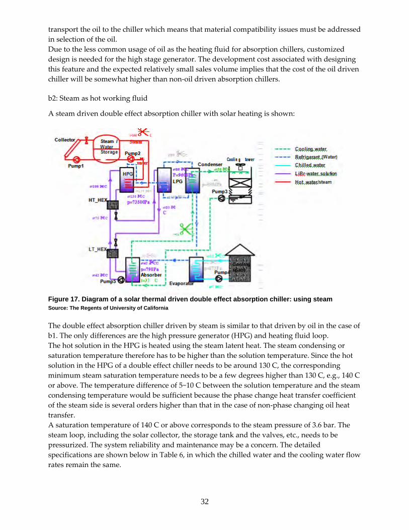
32
transport the oil to the chiller which means that material compatibility issues must be addressed in selection of the oil. Due to the less common usage of oil as the heating fluid for absorption chillers, customized design is needed for the high stage generator. The development cost associated with designing this feature and the expected relatively small sales volume implies that the cost of the oil driven chiller will be somewhat higher than non‐oil driven absorption chillers. b2: Steam as hot working fluid
A steam driven double effect absorption chiller with solar heating is shown:
Figure 17. Diagram of a solar thermal driven double effect absorption chiller: using steam Source: The Regents of University of California The double effect absorption chiller driven by steam is similar to that driven by oil in the case of b1. The only differences are the high pressure generator (HPG) and heating fluid loop. The hot solution in the HPG is heated using the steam latent heat. The steam condensing or saturation temperature therefore has to be higher than the solution temperature. Since the hot solution in the HPG of a double effect chiller needs to be around 130 C, the corresponding minimum steam saturation temperature needs to be a few degrees higher than 130 C, e.g., 140 C or above. The temperature difference of 5~10 C between the solution temperature and the steam condensing temperature would be sufficient because the phase change heat transfer coefficient of the steam side is several orders higher than that in the case of non‐phase changing oil heat transfer. A saturation temperature of 140 C or above corresponds to the steam pressure of 3.6 bar. The steam loop, including the solar collector, the storage tank and the valves, etc., needs to be pressurized. The system reliability and maintenance may be a concern. The detailed specifications are shown below in Table 6, in which the chilled water and the cooling water flow rates remain the same.

33
Table 6. Major design specifications for oil driven solar thermal double effect absorption chillers
Value Unit
Design Specifications (SI) (SI) Remarks
Solar collector capacity 422 kW
Steam heating system efficiency 0.80 Assumed value
HPG solution temperature + 10
Steam saturation temperature 140 C C
Steam saturation pressure 3.6 bar From steam table
Pump flow rate 0.21 kg/s 3.4 GPM
Fixed
Hot water pump type speed Fixed speed is sufficient
Water level should be ~half
Storage tank capacity ~1 m^3 @steady state
Double
Chiller type effect Steam driven
Chiller capacity 120 RT Assumed benchmark capacity
Chiller COP 1.25 A typical value
There is some condensation in
Heating fluid (steam) inlet quality 0.98 the pipe
Slightly above solution
temperature, with some
Heating fluid outlet temperature 135 C subcooling
Heating fluid flow rate 0.17 kg/s 2.7 GPM
HPG solution design temperature 130 C
LPG solution design temperature 80 C
Chilled water leaving temperature 6.7 C Typical design value
Chilled water returning temperature 12.2 C Typical design value
Chilled water flow rate 18.1 kg/s 288 GPM

34
Value Unit
Cooling water leaving temperature 35.0 C Typical design value
Cooling water returning design
temperature 29.4 C Typical design value
Cooling water flow rate 32.7 kg/s 518 GPM
Chiller water charge amount 235 liter 62 gallon
LiBr charge amount 640 liter 169 gallon Source: The Regents of University of California Before the chiller is started, the heating fluid system may be below the working pressure of 3.6 bar. It will take some time to build up the pressure and the overall system start up time may be longer than one hour. This is a major drawback and will significantly limit the use of steam driven absorption chiller.
Solar thermal driven triple effect chilling: oil driven
A triple effect absorption chiller adds another steam generator on top of the two generators in a double effect absorption chiller. The added generator produces more refrigerant steam with the same amount of heating load which translates to a higher COP. Without detailed information on the triple effect chiller design, the following concept of solar thermal driven triple effect cooling is based on the assumption that the solution temperature in the highest stage generator is 160 C. As long as the hot heating fluid temperature is higher than this temperature, the solar collector would be able to drive the triple effect chiller. The system diagram is shown in Figure 19.
Figure 18. Diagram of a solar thermal driven triple effect absorption chiller

35
Source: The Regents of University of California New Energy Development Organization (NEDO) of Japan developed triple effect absorption chillers from 2001‐2004, in cooperation with Japan Gas Association and four major absorption chiller manufactures. With the help of US Department of Energy2, Trane and York each had developed their own triple effect chillers based on the double effect technology (Figure 20). However, no triple effect chillers are commercially available today.
375 Ton 1.6 COP ‐ Trane 400 Ton 1.6 COP ‐ York
Figure 19. Trane and York triple effect chillers Source: The Regents of University of California Compared to an oil driven double effect chiller, the COP of the triple effect is higher. Higher heating fluid temperature means higher loss and lower solar collector efficiency. In addition, triple effect chillers are susceptible to corrosion due to very high solution temperature. The cost of triple effect chillers are also expected to be much higher with a smaller sales volume and possibly higher maintenance costs. Overall, using triple effect chillers today seems a less favorable option than using double effect chillers. Steam may be considered as well to drive triple effect chillers. However, since the solution temperature is even higher, close or above 160 C, the heating steam should be at a pressure close to 9 bar. That makes the steam storage and sealing more difficult. The startup time will be longer than in a steam driven double effect chiller. These are likely to be the show‐stopper for steam driven triple effect chillers.
Table 7. Major design specifications for oil driven solar thermal triple effect absorption chillers
Value Unit
Design Specifications (SI) (SI) Remarks
Solar collector capacity 406 kW
Oil heating system efficiency 0.65 Assumed value
Assume oil supply temperature +
Hot oil outlet temperature 270 C 10C
Design hot oil temperature leaving Assume return oil temperature -

36
Value Unit
storage 160 C 10C
Pump flow rate 1.8 kg/s 29 GPM
Variable
Hot oil pump type speed
Storage tank capacity 6.6 m^3 Assume 1 hour full load supply
Triple
Chiller type effect Oil heating
Chiller capacity 120 RT Assumed benchmark capacity
Chiller COP 1.6 A typical value
Hot oil inlet temperature 260 C 500 F
Hot oil leaving temperature 170 C HPG solution temperature + 10C
Hot oil flow rate 1.5 kg/s 23 GPM
HPG solution design temperature 160 C High pressure generator
MPG solution design temperature 130 C Mid pressure generator
LPG solution design temperature 80 C Low pressure generator
Chilled water leaving temperature 6.7 C Typical design value
Chilled water returning temperature 12.2 C Typical design value
Chilled water flow rate 18.1 kg/s 288 GPM
Cooling water leaving temperature 35.0 C Typical design value
Cooling water returning design
temperature 29.4 C Typical design value
Cooling water flow rate 29.5 kg/s 518 GPM
Chiller water charge amount TBD liter Data unavailable
LiBr charge amount TBD liter Data unavailable Source: The Regents of University of California

37
XCPC driven combined chilling and heating
From the building owner standpoint, it is desirable to use the solar heat for space heating in cold days. This can be conveniently realized by sending a branch of the hot oil into an oil‐water heat exchanger, as shown in the brown box in Figure 21 below.
Figure 20. Diagram of a solar thermal driven combined heating and cooling Source: The Regents of University of California
Combined cooling and heating can be applied to single, double or triple effect chillers in theory. For illustration purposes, we use an oil solar thermal double effect chiller as an example. For the days when cooling demands are high, the hot oil flow to the oil‐water heat changer is closed and the system behaves just the same as b1), the solar thermal driven double effect absorption chiller. In heating days, the hot oil flow going to the HPG of the chiller is closed and the hot oil is sent to the oil‐water heat exchanger. The cooling specifications are the same as in Table 3 for the oil driven double effect chillers. The heating specifications are shown in Table 8. Table 8. Heating mode design specifications for an oil driven solar chilling/heating system
Value Unit
Design Specifications (SI) (SI) Remarks
Solar collector capacity 497 kW
Oil heating system efficiency 0.85 Assumed value
Assumed value to allow good heat

38
Hot oil temperature produced 150 C transfer
Design hot oil temperature leaving Assumed value to allow good heat
storage 100 C transfer
Pump flow rate 5.0 kg/s 79 GPM
Variable
Hot oil pump type speed
Storage tank capacity 17.9 m^3 Assume 1 hour full load supply
(The previous chilled water loop now serves as the space heating water
Heating capacity 422 kW
Heating water leaving temperature 65.0 C Typical design value
Heating water returning temperature 55.0 C Typical design value
Heating water flow rate 10.1 kg/s 160 GPM
(The previous cooling water loop now is disconnected) Source: The Regents of University of California Compared to the cooling case, the solar collector pump flow rate is larger in the heating mode and the heating/chilled water flow rate is lower. Large pump sizes can be chosen such that the pumps satisfy both the cooling and heating needs. Certain double effect chillers are capable of delivering both chilled water and hot water on days when cooling demands are relatively low. XCPC driven ORC Figure 22 shows a potential conceptual architecture for an integrated XCPC/ORC system. The balance of systems components for the architecture is identical to those presented for the previous architectures. There is a possibility that other components and interfaces might emerge as requirements once a detailed design is created (part of a product development activity).

39
Figure 21 Solar ORC conceptual sstem architecture Source: The Regents of University of California The PureCycleTM ORC product offered by UTC Power uses waste heat for power generation and has been demonstrated for geothermal applications with a source heat temperature of < 100 C. Figure 23, shows a picture of the product which uses several components that are already available in volume production.
Figure 22. UTC Power PureCycleTM product
Source: The Regents of University of California The product can currently produce about 220 kW of electricity at approximately ~10% efficiency (thermal to electricity) and there are designs that are currently being developed to increase the generation capacity and improve the efficiency of the system. Solar thermal Rankin cycles have been demonstrated for utility scale operations using solar trough or power tower technology. The advantage of this product is that it is a good fit for distributed power generation applications. Depending on the capabilities of the collector, the design could be further adapted in such a way that exhaust from this system feeds a single or double effect chiller thereby providing a combined cooling, heating and power (CCHP) product. Table 9 presents design parameters for the ORC when fed with 150 C working fluid (hot water) from the XCPC. The parameters presented in the table were obtained from high level models

40
used by UTRC to estimate impact of source temperatures and other design parameters on ORC performance.
Table 9. Major design specifications for XCPC driven ORC cycle
Value Unit
Design Specifications (SI) (SI) Remarks
Calculated assuming 12% cycle
Solar collector capacity 2 MW efficiency for 220 kW
Assumed lower bound in current
design (high temperatures might
Heat source temperature (hot water) 150 C require change of working fluid)
Heat source mass flow rate 38 kg/s Steam flow rate would be ~ 1 kg/s
Heat source exit temperature 130 C
Turbine inlet pressure 20 atm Refrigerant loop
Turbine inlet temperature 124 C Refrigerant loop
Condenser inlet pressure 1.7 atm Refrigerant loop
Condenser inlet temperature 56 C Refrigerant loop
Pump inlet pressure 1.8 atm Refrigerant loop
Pump inlet temperature 28 C Refrigerant loop
Evaporator inlet pressure Refrigerant loop
Evaporator inlet temperature 29 C Refrigerant loop
Electrical power efficiency 12 % Source: The Regents of University of California The current design of the ORC uses a copper evaporator to transfer heat from hot water to the refrigerant. If the working fluid is hot oil, it could conceivably be pumped directly into the existing copper heat exchanger which serves as the evaporator. Corrosion and leakage issues could become a concern in this case. The use of high or low pressure steam also might require some re‐design of this evaporator and this will work its way into the final system cost. In the case where the XCPC collector reaches its target 250 C design goal there is the possibility of creating higher efficiency ORC configurations. Improving efficiencies in this case would require major redesign of all the ORC components to deal with the new refrigerant and the overall system will need to be re‐qualified. Conclusions and Recommendations Conceptual technical system architectures for five major applications of XCPC derived solar energy have been explored in this report and high level engineering estimates point to the fact

41
that designs are technically feasible. A common theme that will impact detailed design for all the architectures is the choice of the working fluid for the collector. This choice could impact heat exchanger designs across all the proposed architectures. The chiller and ORC products today operate at pre‐determined design points and transient behavior of the heat source could have a negative impact on performance and reliability. The use of a thermal storage tank in all the architectures could help abate some of the concerns but it is likely that a supervisory control subsystem would need to be developed to seamlessly integrate the XCPC to the various products. Task Component and Equipment Interfaces for System Integration and on Technical and Economic Performance Requirements for Solar Thermal Collectors Introduction
This report is a complement to the report on preferred system architectures (“Report on Technical System Architectures for Application of Solar Heat”) that summarized some of the conceptual XCPC integrated system architectures and technical features for these architectures. The architectures considered included:
e) XCPC driven single effect chilling
f) XCPC driven double effect chilling
g) XCPC driven triple effect chilling
h) XCPC driven cooling and heating
i) XCPC driven ORC
The previous report focused on products that could be integrated with the XCPC and presented some potential conceptual designs for the complete system. This report focuses around some of the key components and interfaces required to create the integrated system. An emphasis is placed on understanding some of the cost and reliability considerations associated with these systems. This helps guide some of the performance and cost requirements for the XCPC collectors. The cost parameters presented in this report have been estimated using some in house expertise guided cost estimation obtained from various HVAC design manuals. Appendix A presents a summary of these cost estimates for the five configurations (less the collector and storage tank). These numbers will be further validated prior to use in the system modeling analysis task (Task 9) where 24/7 building electric, cooling and heating load data will be used to further determine the economic competitiveness of proposed options. XCPC driven single effect chilling Components and interfaces The system architecture for this concept has been described in some detail in the earlier report. The balance of system components required for this design includes:
• One (or two) pumps to circulate the XCPC working fluid in between the collector and the chiller

42
• A thermal storage tank (hot water or oil) that serves the function of minimizing the
impact of temperature transients in the XCPC working fluid by providing a steady temperature source to the moderate temperature generator of the chiller
• A three way valve that allows bypassing of the storage tank especially when the tank is
full
• A cooling tower (with a fan) and an associated pump used to circulate cool water to the absorber especially in some of the warmer climates
• Supervisory controller that interfaces data collected from the XCPC with chiller
modes of operation so that optimal control decisions are made from a system performance perspective
• A radiator that might also be needed to dump some of additional heat when tanks are
full (also needed from a safety standpoint)
The technical requirements for these chillers indicate that the collector performance should match the heat source specifications provided in the previous report (6.700.0013‐3b). Briefly, the XCPC when coupled with a single effect chiller will only need to provide ~ 92 C. Since this is close to the lower bound temperature for the XCPC, one possibility is to design the collectors at a low cost with capacity of delivering hot water at these temperatures. Alternatively, higher temperatures would mean that the chiller could be used as a bottoming cycle with an intermediate heat exchanger that can generate process fluid capable of driving a thermally activated technology (potentially an ORC) that operates at a higher temperature. This option however would mean that the collector should be capable of heating working fluid entering at 80 C to the higher target temperature (possibly as high as 250 C). This type of hybrid configuration maybe worth considering once the operational capabilities of the XCPC have been demonstrated and qualified. System economics considerations One of the key economic considerations when installing chillers is the impact of parasitic power on the overall value proposition of the system. Parasitic power for chiller includes electrical power needed to run the solution and refrigerant pumps, the fan used in the cooling tower and the chilled water and condenser pumps. Figure 24, shows the anticipated parasitic power required for a single effect chiller at various cooling capacities and distances between the chiller and cooling tower. The numbers are based on engineering estimates arrived at using product literature data and standard HVAC design guidelines. Specifically, Carrier air conditioning system design manual #3 of 12 which includes
• Open and closed pipe sizing and pressure drops for pipe specification including
valves, strainers and fittings.
• Hydraulic pressure drop for each of the sub components reflected in the chiller ‐ condenser and hot water pump energy calculations.
The highest parasitic power consumption for a single effect chiller is in the distant coupled

43
system configuration and this value is roughly 0.35 kW per cooling ton. This implies that a 100 ton system would consume about 35 kW of electrical power and if the system is operated for approximately 2000 hours (average number of hours for a solar energy system) in the year, the total energy consumption is 70000 kWh.1 Single effect chillers range from 100 – 680 RT.
System Parasitic Electric Consumption Sensitivity at full load
On-board solution & refrigerant pumps, tower fan, chilled & condenser pumps) Baseline - Single Effect Absorption Chillers 100 through 680 tons
Cooling Tons Notes: Coupled distance between chiller and farthest AHU / distance between chiller and cooling tower Close = 25 ft / 60 ft, Medium = 200 ft / 100 ft, Distant = 600 ft / 800 ft Chilled water flow 2.4 GPM/Ton, Condenser water flow 3.6 GPM/Ton, 80% Pump efficiency , 5 ft/100ft wg Figure 23. System parasitic power for single effect chillers Source: The Regents of University of California

44
Operating costs for a hot water driven absorption cooling system will also include the costs associated with consumption of this resource in the system. The levelized cost ($/kWh‐economic requirement) of installing and operating the collector should therefore be lower than the cost associated with simply utilizing a hot water thermal source and this could be challenging. 1 Estimated by indexing actual cooling capacity to ARI published gallons per minute and pressure drop ‐ unique to each size chiller. System reliability considerations
Reliability Block Diagram (RBD) for the
Reliability data of
components within each XCPC Driven Single‐Effect Chiller
subsystem
XCPC Driven Chiller (Single‐Effect) System Boundary
1. Solar Collectors 2. Hot-Water 3. Low-Pressure 4. Condenser
Subsystem Storage Tank Generator
5. Evaporator
11. Instrumentation & Controls
(I&C) Subsystem
6. Absorber
10. PLC 9. Three-Way 8. Pumps & Radiator 7. LT HEX
Subsystem Valve Subsystem
Monte Carlo
Simulation System-Level MTBF Probability Density Function and cumulative Distribution Function
Figure 24. System reliability block diagram Source: The Regents of University of California As shown in Figure 25, the reliability block diagram (RBD) for the single‐effect solar‐driven chiller consists of 11 subsystems (modules). Each subsystem contains components and parts with their associated reliabilities expressed by probability density functions (pdf). Each subsystem contains a set of components and parts required for the subsystem to perform a specific function. The subsystem could be a single component such as the condenser, evaporator, or heat exchanger. The subsystem could also be a collection of more than one component, for example, the instrumentation & controls subsystem contains all process proportional–integral–derivative (PID) controllers, level indicators, flow indicators, pressure indicators, process alarms, etc. The reliability of each subsystem is determined by the product of

45
reliabilities of its constituent components and parts. The latter are typically estimated from historical failure rate data of the components and parts within the subsystem. The reliability metrics for most of the components and subsystems associated with the chiller are well known which means the collector subsystem and hot water storage tanks are the components for which the data is currently unavailable. In order for a XCPC integrated system to work, the reliability numbers on the additional balance of system components in this configuration would have to be comparable to reliability numbers for a conventional hot water driven chiller system. A Monte Carlo simulation technique can be used to predict the system‐level reliability (R) by quantifying the reliability block diagram (RBD). The system reliability is the product of its subsystems reliabilities as described by the equation: R = R1.R2.R3.R4.R5.R6.R7.R8.R9.R10.R11, where R1, R2, R3 ... etc represents the reliability of subsystem 1, 2, 3, etc, respectively. The predicted system‐level reliability is typically measured by the mean time between failures (MTBF). As the Monte Carlo simulation allows for propagation of uncertainties in the reliabilities of the various subsystems, the predicted system‐level MTBF will be given in the form of a probability density function with a mean value (best estimate), standard deviation, lower bound, and upper bound values. This simulation can be performed as part of a detailed design effort once the metrics of performance and reliability have been clearly established for the XCPC collectors. These reliability results should help identify then estimate some of the maintenance costs that could be required for the system. XCPC driven double effect chilling Components and interfaces The components and interfaces required to design an integrated XCPC and double effect chiller system are identical to those required for a single effect chiller with the possibility of the following additions:
a. A compressor if high pressure steam is used as the input into the high temperature generator (preferred for 16DE design)
b. A heat exchanger that is adequately integrated into the high temperature generator if heat transfer fluid such as hot oil becomes the working fluid of choice
The first choice is not preferred due to regulatory complexity (steam codes). Maintaining the temperature of the fluid entering the high temperature generator (at approximately 200 C) is of great importance in the second system configuration because this enables operation at the optimized design point. A system that works with a collector and hot storage tank front end may be inadequate in maintaining this temperature especially during transient operation. This suggests the possible need for a supplemental burner to provide heat to the generator in case the designed front end does not work adequately. The decision on adding this component will greatly depend upon the target capacity of the chiller and the type of building that the integrated system will service. There may be some additional complexity needed in the supervisory control to allow for functioning of the chiller using the supplemental burner.

46
System economics considerations Double chillers are sized between 70 – 520 RT. System parasitics (pumps, cooling towers etc.) are a consideration for double effect chillers as well. Figure 26, summarizes these as a function of cooling capacity and distance. Energy consumption is in the range of 0.45/kW (versus 0.35/kW) for single effect systems. Known high pressure double effect chillers are more fully optimized than low pressure single effect chillers. On‐board parasitic losses are actually comparable for single effect and double effect machines with the latter having the added benefit of a higher COP. External pump, tower fan and other auxiliary power consumption however are higher for the double effect chiller. This penalty could trade favorably against the improved chiller COP
. Figure 25. System parasitic power for double effect chillers Source: The Regents of University of California Double effect chillers can work with steam or on natural gas with the latter being more common due to avoidance of high pressure steam in several buildings. The yearly operating costs for a natural gas driven system would therefore in large part include the yearly fuel consumption (natural gas price * volume) incurred by the customer. This implies that in order for a system to be economically viable, the overall capital cost incurred by the XCPC plus balance of systems should be recovered through deferral of fuel costs. The economics of the system consequently changes substantially with increased fuel costs. Assuming a 300 kW cooling requirement, a double effect chiller operating at a COP of 1.1 would require ~273 kW of thermal energy or ~546,000 kWh (assuming 2000 hours of operation). At $0.04/kWh ($12/mm BTU) natural gas cost, yearly fuel savings from an XCPC system would be ~$22,000 which means that the cost of the XCPC plus balance of systems should be no more than $100,000 to have a simple payback of 5 years (assuming the chiller equipment already exists in the building). In order to obtain 273 kW of thermal energy, the XCPC field should be ~550 m2 (assume 0.5 kW/m2 collected) which

47
means that the $/m2 for a fully installed collector field should be well under $200/m2 to create a reasonable value proposition. The system’s competitiveness is even more challenging if the building uses electrically driven vapor compression systems that have a COP which is about three times higher than thermally driven processes. In such a scenario, a chiller that provides 300 kW of cooling requires only 100 kW (at a COP of 3) of electricity. A system that operates over a year would consume ~200,000 kWh (assuming 2000 hours of operation) that translates to yearly costs (at $0.20/kWh) of ~$40,000. The total system (including cost of replacement absorption chiller) should therefore cost no more than $200,000 to have a simple payback of 5 years2. Electric chillers can be considered as having an emission footprint associated with the electricity (typically derived from coal plants) required to drive the cooling process. Double effect chillers running on natural gas could have a lower carbon foot print and the advantage is enhanced when using solar energy as the heat source. The economics for the systems would therefore be more favorable when the cost of natural gas is higher and when additional benefits are realized by applying carbon credits.
Figure 26. System Parasitic Electric Consumption Sensitivity at full load Source: The Regents of University of California

48
Figure 27. Reliability block diagram XCPC driven double effect chillers Source: The Regents of University of California
2 Note: These are simple high level calculations. Actual economics depends on system performance and real building loads that will be part of Task 5 assessment.
Compared to the single‐effect solar‐driven chiller which has 11 subsystems, the reliability block diagram (RBD) for the double‐effect (hot oil) solar‐driven chiller consists of 13 subsystems (modules) primarily due to the increased number of components within the chiller. The reliability expression will have two additional terms that correspond to this increased part count. Typically from a reliability perspective, increase part count results in lower reliability for the system. Besides the reliability metrics for the XCPC collector, the metrics for the hot oil / steam storage tank are also an unknown at this point. Additionally, if there is any alteration that is made to the high pressure generator (e.g. to make it compatible with hot oil), the reliability numbers for this design will need to be collected. XCPC driven triple effect chilling Components and interfaces The system that uses the XCPC integrated with a triple effect chiller would be identical to the double effect chiller option in terms of the balance of system components required for integration with the XCPC. There may be significant redesign required for the high temperature generator to make it compatible with hot oil. Since triple effect chillers are not commercially available in volume, the non recurring engineering has not been sunk into a sub optimal design. The system will also require a supplemental burner and additional control logic (similar to

49
requirements for the double effect chiller) to facilitate seamless performance during transient operation of the solar thermal collectors. System economics considerations The parasitic power associated with on‐board electrical consumption (not including remote pumps or a cooling tower) for the three different types of chillers have been summarized in Figure 29. Since there is limited actual data on the triple effect devices, the electrical parasitic power for this application have been projected based on high level system parameters that were gathered in the previous report (Task 3 report 6.700.0013‐3a).
Figure 28. On board parasitics for chillers Source: The Regents of University of California
The total parasitic power for the triple system benefits from derivation from the double effect machines but will likely consume more energy. The economic competitiveness of triple effect chillers compared to the double effect has not yet been validated. The higher COP of these systems could result in ~30% lesser consumption of fuel but the increased complexity of the system could increase maintenance costs thereby diminishing the value proposition for the small capacity chiller systems. System reliability considerations The reliability block diagram (Figure 30) for the XCPC driven triple effect chiller shows that the part count in this system has gone up by an additional two components. The concerns about LiBr temperature controllability and the effect of increased temperature induced corrosion problems make this system less desirable from a reliability perspective. Redesign of the HPG to be compatible with hot oil will also add uncertainty in the final reliability numbers for the system.

50
Figure 29. Reliability block diagram XCPC driven double effect chillers Source: The Regents of University of California XCPC driven cooling and heating Components and interfaces The components and interfaces required for this configuration are largely the same as the double effect configuration. There could be the need for an intermediate heat exchanger that is used to provide the hot water supply to the building. This might require some change in the control logic of the supervisory control for the system which enables managing demand side management for the cooling and heating needs of the building. System economics consideration The integrated system would only be marginally more expensive than the double effect configuration (see Appendix A). This would be the case if a secondary heat exchanger is used to obtain the hot water and if there is plumbing required to interface the system with existing building hot water supplies. There are chillers available that can operate in dual mode (both cooling and heating) which could be ideal for situations where the cooling load is low (mild summer days). Providing heating to the building could help defer fuel costs (natural gas) if heating is provided through traditional boilers or electricity costs if the building uses electrical heating. The latter would be more favorable from a value proposition standpoint given the higher cost of electricity (in general) compared to the cost of natural gas and the lower cost of strip electric resistance heaters to hydronic boiler assisted systems.

51
System reliability considerations The addition of a heat exchanger and additional plumbing to the double effect configuration would add one more component to the reliability equation and this also introduces another point of failure for the system. The failure will likely not be catastrophic since the default of any controller would be to revert to existing back up hot water lines to meet the requirements of the building in case the heating subsystem in the configuration fails. XCPC driven ORC Components and interfaces The components and interfaces required for the XCPC driven ORC configuration are identical to those considered for the double effect chiller option. The choice of thermal oil is the most attractive option from an ease of integration and implementation standpoint. The technical requirements dictate that roughly 2 MW of thermal energy at 150 C must be supplied to the ORC evaporator to obtain approximately 200 kW of electric power. The ORC supervisory controller may need to be modified to operate at part load under transient solar insolation conditions. The variable speed controller on the working fluid pump for the current ORC enables operation at part load. System economics considerations The economics of an XCPC driven ORC should be compared to the most common method for obtaining distributed solar electricity namely solar PV. The volume cost of an ORC unit is projected at $2.7/W (installed). The total cost (installed) for the integrated system could therefore be in the neighborhood of $4/W today (approximately half the cost of an installed PV system). This system assuming 50% total collection efficiency and 20% ORC efficiency would operate at a net efficiency of 10% which is comparable in efficiency to installed PV systems today implying that the overall electricity generated by the system could be equivalent to that provided by identically sized PV systems. The main deficiency in the ORC concept is that the moving parts associated with the machine and the overall system could result in higher maintenance costs compared to flat panel PV systems thereby reducing the factor of 2 advantages on levelized energy costs (realized through reduced system capital costs). System reliability The block diagram presented in Figure 31, is a simplified picture of the overall XCPC driven ORC concept because it uses a single subsystem to represent the ORC which is itself comprised of 5 or more components. It is represented this way because it is conceivable that no modification is required to interface the system with hot water, steam or oil (not true for chillers where some modification of generator heat exchangers may be required). In any event, the ORC reliability number would be a product of the reliability of the individual components that comprise the system and the total number of “parts” for the integrated system would be in the range of that for the double effect chiller configuration. The uncertainty in reliability metrics is again primarily associated with the solar collector subsystem and the storage tank component. There is the additional possibility that the reliability metrics for ORC components might change should the refrigerant be altered to achieve higher system efficiencies.

52
Figure 30. Reliability block diagram XCPC driven ORC Source: The Regents of University of California Conclusions and recommendations Analyzing the XCPC integrated system architecture options from a components, interfaces and economics perspective shows that there could be major challenges in launching these systems. All these systems require additional off the shelf components and interfaces compared to traditional methods of implementing the product. The ability of the XCPC to achieve cost targets of less than $100/m2 with minimal maintenance costs coupled with increases in fuel and other utility costs will largely dictate the economic attractiveness of the various systems. Estimation of system maintenance costs will be contingent upon high level reliability metrics for the integrated systems.
Based on the current analysis3, it is recommended that system modeling and economic viability calculations focus on the double effect chiller and solar ORC configuration. It is also recommended that UC Merced provide UTRC with specifications of the working fluid, collector costs (and breakdown) and collector reliability so that some of these elements can be incorporated into the system and economic modeling tasks that will follow as part of Task 5.

53
3 Analysis conducted by synthesizing real world experience from interviews with service contractors, professionals, reviewing long term proprietary service records Table 10. Equipment cost estimates (less collector, storage tank and front end collector to tank piping)
Source: The Regents of University of California
2.2.2. Safety Considerations for XCPC Applications This report summarizes some of the main safety considerations for system architectures that have been discussed extensively in the two previous reports of Task 3 (“Report on Technical System Architectures for Application of Solar Heat” and “Report on Component and Equipment Interfaces for System Integration and on Technical and Economic Performance Requirements for Solar Thermal Collectors”). This report summarizes the safety considerations in terms of two broader categories: a) XCPC driven absorption cooling, b) XCPC driven ORC. XCPC driven absorption cooling Safety considerations for XCPC driven absorption cooling/heating technologies are mainly associated with three sources: 1) heating fluid with high temperature and/or high pressure; 2) corrosive LiBr solution in absorption chillers; and 3) general equipment malfunctioning such as motor winding high temperature and leakage of hermetic pumps. The degree of safety concerns varies with the system configuration. Here we will focus on configuration specific safety issues, i.e., 1) & 2) only.

54
Solar thermal driven single effect chilling In this system, the hot water is below 100 C and at atmospheric pressure. The solution temperature in the single effect chiller is low. Both the chiller and the solar collector are mature technologies, thus this configuration has the least safety concern. Solar thermal driven double effect chilling (b1: oil or b2: steam as hot working fluid) Direct fired or steam driven double effect chillers are also mature technologies and are not of great safety concerns. Major concern comes from the fact that hot oil needed to drive the double effect chiller may leak into the solar collector or the LiBr solution in the HPG. For steam driven system, the safety issue arises when the heating fluid loop, including the solar collector, the water storage tank and the pump, all need to be pressurized to approximately 3.6 bar. The pressurization cycle will have a daily cycle, a severe condition for a pressurized system. This may drive system configuration to a hot oil temperature. Solar thermal driven triple effect chilling For triple effect chillers, assuming hot oil is used, the oil temperature needs to be even higher. Possible leakage or contact with the oil becomes more dangerous and poses an increased safety concern than the double effect chillers. In addition, the solution in triple effect chillers, with much higher temperature, becomes very corrosive. The piping, valve, pump and heat exchanger life are likely to be affected. Possible spill of the solution can be a great safety hazard. Solar thermal driven combined chilling and heating Heating option in the solar driven chillers does not add any significant safety concerns because the modification to the system is minimal, consisting of a plate heat exchanger and valves. These technologies are simple and mature. XCPC driven ORC The choice of the XCPC working fluid will also impact some of the safety considerations in the integrated ORC system design. The use of hot oil will require appropriate design of lines and storage devices so that leaks are minimized (particularly important for roof top applications where there may be no access to drains). The use of high pressure steam as the working fluid may be less problematic from a safety aspect since there are several existing examples of high pressure steam being pumped in and out of buildings for heating purposes. The refrigerant used in the ORC could become a source of future safety/environmental considerations. Phase out of chloro‐fluoro carbon based refrigerants might occur and this coupled with the need to adapt the design to higher efficiencies could mean the use of newer refrigerants that will need to be qualified for safety. Conclusions and recommendations Current assessment of the XCPC integrated systems indicates that the choice of the working

55
fluid through the collector will be the most important safety consideration in system design. Storage and buffering conveniences associated with the ability to thermal cycle and the stringent requirements on steam code might drive towards the design choice of hot oil. It is recommended that the hot oils be selected only after it is completely clear that there are no existing or emerging regulatory bans that are imminent on these substances. This may require doing some assessment work with the California Environmental Protection Agency (EPA) prior to down selecting the preferred working fluid.
2.3. Task 4.0 The design team (SolFocus and UC‐Merced) formulated three competing conceptual level designs for the External Compound Parabolic Concentrator (XCPC) that is to be developed during the course of this project. All three designs are believed to have the potential to reach the performance and cost goals defined in the agreement, which are to develop a manufacturable stationary solar thermal collector system with a system efficiency of at least 50 percent at a temperature of 400ºF, and also have a production cost of less than $10 per square foot. Each of the formulated designs consists of an assembly of stationary evacuated tube absorbers with external non‐imaging reflectors. The three competing design concepts that have been formulated are:
1. All glass dewar: Direct Flow
2. All glass dewar filled with thermal fluid: Indirect Flow
(a) with metal tube
(b) with heat pipe
3. Metal absorber with glass‐to‐metal seal
(a) with metal tube
(b) with heat pipe
Concept 1 ‐ All glass dewar: Direct Flow
The design concept is depicted in Figure 32. The heat transport fluid flows directly inside the all‐glass dewars – hence we use the term “direct flow”. The design concept uses very inexpensive all glass Dewar solar thermal absorbers that are mass produced in China. The dewars are cylindrical borosilicate glass bottles with an evacuated annulus between the two glass walls. The vacuum surface of the inner wall is coated with a selective surface (usually aluminum nitride cermet) with a high solar absorptance and low thermal emittance. Popular dimensions of off‐the‐shelf Chinese Dewars are 44mm (inside diameter), 58mm (outside diameter) and 1800mm length. Other Dewar dimensions are also available. The glass dewars are to be attached to a plumbing manifold using O‐ring compression seals. The manifold will incorporate a unique design feature – the inlet tube (item 8 in Figure 32) will be integral to the manifold itself. This eliminates the need for a separate part (the inlet tube), which speeds field

56
installation and also eliminates a potential leak path (at the connection of the inlet tube to the manifold). Each dewar is placed so that an external reflector concentrates the solar irradiance onto the inner dewar wall of with the selective coating. The shape of the reflector is designed so that all sunlight incident on the aperture plane of the collector within a defined angular acceptance angle is redirected onto the absorber. The acceptance angle can be designed according to the desired concentration factor, the concentrated flux profile and the orientation of the absorber tubes (East‐West or North‐South/tilted). Orienting the absorber tubes North‐South requires larger acceptance angles to ensure sufficient illumination throughout the day, which reduces the concentration factor. Therefore, an East‐West orientation is generally advantageous. However, a North‐South oriented reflector (with the larger acceptance angle) does accept more diffuse solar irradiation and so too has some positive performance attributes. Additionally, reflectors with larger acceptance angles will generally require less reflector area, which provides an economic advantage. Designs for both East‐West and North‐South orientations will be designed and evaluated as part of this project. To achieve our collector cost goals, the reflector must also be low in cost and be easily shaped into the desired CPC profile. And to produce the desired optical performance, the reflectance of the reflective surface must be high (preferably in the ‘90’s). Various reflector materials will be examined and evaluated as part of this project. Also an optional glass or plastic glazing will be considered to cover the reflector and absorbers. The heat transfer fluid (e.g. mineral oil) will be circulated through the absorber tubes. The flow pattern may be in series, in parallel, or a combination of both. The fluid will enter the glass dewar from the manifold, through the inlet tube into the lower part of the absorber tube and will then flow back to the upper end of the dewar in a counter flow direction where it will reenter the manifold. The flow pattern may be such that either the cold or the hot fluid enters through the center inlet tube. Also, the direction of the outlet flow (#3 in Figure 1) may also be configured in the opposite direction. This may offer thermal advantages as well as provide more convenient plumbing connections since the outlet of one collector would then feed into the inlet of an adjacent collector. The manifold may be as depicted in Figure 1 (a tube in a tube) or, as two separated tubes (one supply and the other the return). Analysis of all these options will help us assess the preferred configuration. Features
Heat Transfer: This design is expected to have excellent heat transfer from the black selective surface to the working fluid because the heat collected on the coated wall of the inner dewar has only to conduct through the inner dewar wall (typically 2mm thick) to reach the circulating working fluid that flows in the dewar. Cost: This design is very likely to be the lowest cost option of the three competing designs in terms of material cost. However, the operating cost (pumping) may suffer slightly due to the counter flow path and the larger pressure drop where the flow reverses in direction. If that becomes an issue, the design can be modified to reduce pressure drop. Manufacturability: This design is amenable to low cost manufacturing. Installation: This design is very easily installed as the dewars can be attached to the manifold on site. Broken dewars can be easily replaced. Orientation: This design allows all possible tube orientations (East‐West, North‐South). Robustness: The fluid is circulated in double‐walled glass dewars so leakage will occur if both dewar walls break. The risk can be reduced by adding safety valves and/or covering the tubes in a box/framework. The concept of solar collectors using all‐glass evacuated tubes is not

57
entirely new. Schott Inc. manufactures and sells all‐glass ICPC collectors and the collectors passed the required performance and safety tests. However, the Schott collectors do not utilize external reflectors, not do they have a tube inlet (part #8) that is integral with the manifold. Durability: Potential durability issues may be glass breakage due to thermal shock and/or temporary pressure surges within the circulating flow stream. In the event of collector stagnation, the dewar surfaces coated with the selective coatings can achieve temperatures in excess of 500oF. Should cold working fluid be suddenly introduced into very hot dewars, it is possible that thermal shock could result in dewar breakage. Another durability concern with this design is the pressure limitation (about 90 psi) imposed by the use of glass as a containment vessel for the circulating working fluid. The durability and/or integrity of the O‐ring compression seals, which are exposed to high and fluctuating temperature, are a concern. All of these various durability issues will be addressed during the performance of this project. Technical Risk: We consider the technical risk of this concept to be reasonably low since heat transfer from the absorber coating to the circulating working fluid is expected to be excellent (i.e. very little thermal resistance along this thermal path) and also because the manifold design is relatively straightforward (although there are a variety of possible design permutations that must be assessed). But, the durability issues identified above are of real and practical concern, so some technical risk is present Concept 2 ‐ All glass dewar filled with thermal fluid: Indirect Flow This design concept allows for two versions: (a) with a metallic tube insert (see Figure 2a); and (b) with a heat pipe insert (see Figure 2b). Both versions of this concept use the same inexpensive all glass Dewar solar thermal absorber tubes as our concept 1. However, in this concept the circulating fluid does not directly contact the glass dewars. The circulating fluid is confined to the manifold and the metallic tubes reaching into the glass dewars (as in version a), or confined to just the manifold itself (as in version b). In both cases the metallic inserts are immersed within a thermal fluid (e.g. a mineral oil) in order to enhance thermal transport from the blackened/coated inner dewar to the metallic insert. Prior research has shown that thermal transport from the dewar to these kinds of thermal inserts is poor because of the poor thermal contact between the inserts and the glass dewars. The addition of the thermal fluid is aimed at greatly enhancing the heat transfer because the thermal fluid will have much better thermal conductivity than does the thin air gaps that are present when the inserts are simply placed inside dry dewars. Another simple variation of this design concept is to use highly‐viscous thermal grease rather than a thermal fluid. Version (a) uses metal tubes to direct the circulating fluid into the dewars to remove the thermal energy. The metal tubes are immersed into a heat transfer fluid to enable and enhance heat transfer from the coated dewar wall to the metallic tube. The tubes may be configured as a “double‐D” (as depicted in Figure 2a) or as a simple bent u‐tube (not shown). The size and shape of these metallic tubes (part #8 in Figure 2a) will be evaluated from the perspective of heat transport, pressure drop and cost before a selection is finalized. These immersed tubes may also have fins attached to enhance thermal performance, and we will also consider minimization of the needed thermal fluid Version (b) uses heat pipes to transfer the heat from the coated dewar to the manifold. Similar to version (a), the heat pipes are immersed in a heat transfer fluid to enable and enhance heat transfer from the coated dewar wall to the heat pipe. Heat pipes of this basic design are

58
currently mass produced in China, but to our knowledge no one has successfully enhanced the thermal transport with the addition of thermal fluid or thermal grease. The absorber tubes are placed so that external reflectors concentrate sunlight onto the evacuated dewars, just as in concept 1. Features Heat Transfer: The heat transfer in this design will not be as good as in our concept 1. The heat has to pass from the coated Dewar wall through three barriers to reach the circulating fluid: The inner glass Dewar wall, the thermal fluid, and the wall of the metal tube/heat pipe. The limiting factor will be the conduction/natural convection through the non‐circulating thermal fluid. Also, with design 2b (the heat pipe design) the operation and performance of the heat pipe is unknown at this point. The heat pipes that are produced in volume in China are used at much lower temperatures than we need, and performance/operation data at the higher operating temperatures is unavailable. Concerns are the “dry out” temperature of these standard heat pipes as well as whether their performance deteriorates significantly as operating temperatures increase. Cost: This design is likely to have low production cost, albeit not as low as our concept 1. However, pumping cost should be lower, especially for design 2b since the use of the heat pipe eliminates all the pressure drop aside from that of the manifold. Manufacturability: This design is amenable to low cost manufacturing. Installation: This design is not as easy to install as concept 1 as the dewars have probably to be filled on site with the thermal fluid. Orientation: This design restricts the possible tube orientation to North‐South as the tubes have to be tilted to keep the thermal fluid from spilling. The North‐South orientation requires a higher optical acceptance angle which reduces the concentration. Robustness: The heat transfer fluid contained in the Dewars is in contact with air. It will be important to select a heat transfer fluid with a flash point above the stagnation temperature of the collector. Some form of container will be needed to prevent spilling of the heat transfer fluid. Oil expansion issues have to be considered. Alternatively, a thermal grease (if found to work sufficiently well) will Durability: Version (a) of this concept is expected to be very durable. The same applies to version (b) assuming satisfactory heat pipe longevity. Since the glass dewars are not used to contain the circulating fluid, there is no risk of dewar breakage in the event of pressure surges within the circulating fluid loop. Similarly, thermal shock is greatly minimized (probably eliminated) because the thermal fluid within the dewars will act to dampen thermal transport. Technical Risk: The technical risk of this concept is higher than concept 1. Potential technical barriers are the heat transfer and the performance and longevity of heat pipes operated at high temperatures. Concept 3 ‐ Metal absorber with glass‐to‐metal seal This concept allows for two versions: (a) with metal tube (see Figure 3a); and (b) with heat pipe (see Figure 3b). In both versions an evacuated glass tube with an innovative glass‐to‐metal seal is used to insulate the metal absorber. The metal absorber is a thin cylindrical copper fin with a selective coating that enables high solar absorptance and reduces radiative heat loss. The fin is welded to a metal counter flow tube (version a) or a heat pipe (version b). In version (a) the heat

59
absorbed by the fin is transferred to the manifold by the circulating fluid in the metal tube. In version (b) the heat is transferred from the fin to the manifold by a heat pipe. The absorber tubes are placed so that external reflectors concentrate sunlight onto the evacuated dewars, just as in concepts 1 and 2. Features Heat Transfer: This design has good heat transfer, but not as good as concept 1 because the absorbed thermal energy must be conducted around a metallic fin before it passes into the working fluid. Cost: This design is likely to have higher production costs than concepts 1 and 2. This is due to the high metal content and especially the glass‐to‐metal seals. Pumping cost might be an issue with the counter flow metal tube of version (a). In this case, a metal U‐tube could be used instead. Manufacturability: The manufacturing is more complex than in concepts 1 and 2. Installation: Version (b) is very easy to install as the heat pipes can be plugged onto the manifold on site. Version (a) requires plumbing. Orientation: Version (a) can be oriented East‐West or North‐South. Version (b) needs some tilt because of the heat pipes. Robustness: The concept is very robust. The fluid is contained in metal pipes. Durability: Thermal stress issues and the longevity of the glass‐to‐metal seals have to be analyzed. Technical Risk: Version (a) has very little technical risk. Version (b) has higher technical risk due to the unknown performance and longevity of heat pipes operated at high temperatures. The design team (SolFocus and UC‐Merced) formulated three competing conceptual level designs for the External Compound Parabolic Concentrator (XCPC) that is to be developed during the course of this project. All three designs are believed to have the potential to reach the performance and cost goals defined in the agreement, which are to develop a manufacturable stationary solar thermal collector system with a system efficiency of at least 50 percent at a temperature of 400ºF, and also have a production cost of less than $10 per square foot. Each of the formulated designs consists of an assembly of stationary evacuated tube absorbers with external non‐imaging reflectors. The three competing design concepts that have been formulated are:
4. All glass dewar: Direct Flow
5. All glass dewar filled with thermal fluid: Indirect Flow (a) with metal tube (b) with heat pipe
6. Metal absorber with glass‐to‐metal seal (a) with metal tube (b) with heat pipe Concept 1 ‐ All glass dewar: Direct Flow The design concept is depicted in Figure 1. The heat transport fluid flows directly inside the all‐glass dewars – hence we use the term “direct flow”. The design concept uses very inexpensive all glass Dewar solar thermal absorbers that are mass produced in China. The dewars are

60
cylindrical borosilicate glass bottles with an evacuated annulus between the two glass walls. The vacuum surface of the inner wall is coated with a selective surface (usually aluminum nitride cermet) with a high solar absorptance and low thermal emittance. Popular dimensions of off‐the‐shelf Chinese Dewars are 44mm (inside diameter), 58mm (outside diameter) and 1800mm length. Other Dewar dimensions are also available. The glass dewars are to be attached to a plumbing manifold using O‐ring compression seals. The manifold will incorporate a unique design feature – the inlet tube (item 8 in Figure 1) will be integral to the manifold itself. This eliminates the need for a separate part (the inlet tube), which speeds field installation and also eliminates a potential leak path (at the connection of the inlet tube to the manifold). Each dewar is placed so that an external reflector concentrates the solar irradiance onto the inner dewar wall of with the selective coating. The shape of the reflector is designed so that all sunlight incident on the aperture plane of the collector within a defined angular acceptance angle is redirected onto the absorber. The acceptance angle can be designed according to the desired concentration factor, the concentrated flux profile and the orientation of the absorber tubes (East‐West or North‐South/tilted). Orienting the absorber tubes North‐South requires larger acceptance angles to ensure sufficient illumination throughout the day, which reduces the concentration factor. Therefore, an East‐West orientation is generally advantageous. However, a North‐South oriented reflector (with the larger acceptance angle) does accept more diffuse solar irradiation and so too has some positive performance attributes. Additionally, reflectors with larger acceptance angles will generally require less reflector area, which provides an economic advantage. Designs for both East‐West and North‐South orientations will be designed and evaluated as part of this project. To achieve our collector cost goals, the reflector must also be low in cost and be easily shaped into the desired CPC profile. And to produce the desired optical performance, the reflectance of the reflective surface must be high (preferably in the ‘90’s). Various reflector materials will be examined and evaluated as part of this project. Also an optional glass or plastic glazing will be considered to cover the reflector and absorbers. The heat transfer fluid (e.g. mineral oil) will be circulated through the absorber tubes. The flow pattern may be in series, in parallel, or a combination of both. The fluid will enter the glass dewar from the manifold, through the inlet tube into the lower part of the absorber tube and will then flow back to the upper end of the dewar in a counter flow direction where it will reenter the manifold. The flow pattern may be such that either the cold or the hot fluid enters through the center inlet tube. Also, the direction of the outlet flow (#3 in Figure 1) may also be configured in the opposite direction. This may offer thermal advantages as well as provide more convenient plumbing connections since the outlet of one collector would then feed into the inlet of an adjacent collector. The manifold may be as depicted in Figure 1 (a tube in a tube) or, as two separated tubes (one supply and the other the return). Analysis of all these options will help us assess the preferred configuration. Features Heat Transfer: This design is expected to have excellent heat transfer from the black selective surface to the working fluid because the heat collected on the coated wall of the inner dewar has only to conduct through the inner dewar wall (typically 2mm thick) to reach the circulating working fluid that flows in the dewar.

61
Cost: This design is very likely to be the lowest cost option of the three competing designs in terms of material cost. However, the operating cost (pumping) may suffer slightly due to the counter flow path and the larger pressure drop where the flow reverses in direction. If that becomes an issue, the design can be modified to reduce pressure drop. Manufacturability: This design is amenable to low cost manufacturing. Installation: This design is very easily installed as the dewars can be attached to the manifold on site. Broken dewars can be easily replaced. Orientation: This design allows all possible tube orientations (East‐West, North‐South). Robustness: The fluid is circulated in double‐walled glass dewars so leakage will occur if both dewar walls break. The risk can be reduced by adding safety valves and/or covering the tubes in a box/framework. The concept of solar collectors using all‐glass evacuated tubes is not entirely new. Schott Inc. manufactures and sells all‐glass integrated compound parabolic collector (ICPC) collectors and the collectors passed the required performance and safety tests. However, the Schott collectors do not utilize external reflectors, not do they have a tube inlet (part #8) that is integral with the manifold. Durability: Potential durability issues may be glass breakage due to thermal shock and/or temporary pressure surges within the circulating flow stream. In the event of collector stagnation, the dewar surfaces coated with the selective coatings can achieve temperatures in excess of 500oF. Should cold working fluid be suddenly introduced into very hot dewars, it is possible that thermal shock could result in dewar breakage. Another durability concern with this design is the pressure limitation (about 90 psi) imposed by the use of glass as a containment vessel for the circulating working fluid. The durability and/or integrity of the O‐ring compression seals, which are exposed to high and fluctuating temperature, are a concern. All of these various durability issues will be addressed during the performance of this project. Technical Risk: We consider the technical risk of this concept to be reasonably low since heat transfer from the absorber coating to the circulating working fluid is expected to be excellent (i.e. very little thermal resistance along this thermal path) and also because the manifold design is relatively straightforward (although there are a variety of possible design permutations that must be assessed). But, the durability issues identified above are of real and practical concern, so some technical risk is present Concept 2 ‐ All glass dewar filled with thermal fluid: Indirect Flow This design concept allows for two versions: (a) with a metallic tube insert (see Figure 2a); and (b) with a heat pipe insert (see Figure 2b). Both versions of this concept use the same inexpensive all glass Dewar solar thermal absorber tubes as our concept 1. However, in this concept the circulating fluid does not directly contact the glass dewars. The circulating fluid is confined to the manifold and the metallic tubes reaching into the glass dewars (as in version a), or confined to just the manifold itself (as in version b). In both cases the metallic inserts are immersed within a thermal fluid (e.g. a mineral oil) in order to enhance thermal transport from the blackened/coated inner dewar to the metallic insert. Prior research has shown that thermal transport from the dewar to these kinds of thermal inserts is poor because of the poor thermal contact between the inserts and the glass dewars. The addition of the thermal fluid is aimed at greatly enhancing the heat transfer because the thermal fluid will have much better thermal conductivity than does the thin air gaps that are present when the inserts are simply placed inside dry dewars. Another simple variation of this design concept is to use highly‐viscous thermal grease rather than a thermal fluid.

62
Version (a) uses metal tubes to direct the circulating fluid into the dewars to remove the thermal energy. The metal tubes are immersed into a heat transfer fluid to enable and enhance heat transfer from the coated dewar wall to the metallic tube. The tubes may be configured as a “double‐D” (as depicted in Figure 33) or as a simple bent u‐tube (not shown). The size and shape of these metallic tubes (part #8 in Figure 33) will be evaluated from the perspective of heat transport, pressure drop and cost before a selection is finalized. These immersed tubes may also have fins attached to enhance thermal performance, and we will also consider minimization of the needed thermal fluid Version (b) uses heat pipes to transfer the heat from the coated dewar to the manifold. Similar to version (a), the heat pipes are immersed in a heat transfer fluid to enable and enhance heat transfer from the coated dewar wall to the heat pipe. Heat pipes of this basic design are currently mass produced in China, but to our knowledge no one has successfully enhanced the thermal transport with the addition of thermal fluid or thermal grease. The absorber tubes are placed so that external reflectors concentrate sunlight onto the evacuated dewars, just as in concept 1. Features Heat Transfer: The heat transfer in this design will not be as good as in our concept 1. The heat has to pass from the coated Dewar wall through three barriers to reach the circulating fluid: The inner glass Dewar wall, the thermal fluid, and the wall of the metal tube/heat pipe. The limiting factor will be the conduction/natural convection through the non‐circulating thermal fluid. Also, with design 2b (the heat pipe design) the operation and performance of the heat pipe is unknown at this point. The heat pipes that are produced in volume in China are used at much lower temperatures than we need, and performance/operation data at the higher operating temperatures is unavailable. Concerns are the “dry out” temperature of these standard heat pipes as well as whether their performance deteriorates significantly as operating temperatures increase. Cost: This design is likely to have low production cost, albeit not as low as our concept 1. However, pumping cost should be lower, especially for design 2b since the use of the heat pipe eliminates all the pressure drop aside from that of the manifold. Manufacturability: This design is amenable to low cost manufacturing. Installation: This design is not as easy to install as concept 1 as the dewars have probably to be filled on site with the thermal fluid. Orientation: This design restricts the possible tube orientation to North‐South as the tubes have to be tilted to keep the thermal fluid from spilling. The North‐South orientation requires a higher optical acceptance angle which reduces the concentration. Robustness: The heat transfer fluid contained in the Dewars is in contact with air. It will be important to select a heat transfer fluid with a flash point above the stagnation temperature of the collector. Some form of container will be needed to prevent spilling of the heat transfer fluid. Oil expansion issues have to be considered. Alternatively, a thermal grease (if found to work sufficiently well) will Durability: Version (a) of this concept is expected to be very durable. The same applies to version (b) assuming satisfactory heat pipe longevity. Since the glass dewars are not used to contain the circulating fluid, there is no risk of dewar breakage in the event of pressure surges

63
within the circulating fluid loop. Similarly, thermal shock is greatly minimized (probably eliminated) because the thermal fluid within the dewars will act to dampen thermal transport. Technical Risk: The technical risk of this concept is higher than concept 1. Potential technical barriers are the heat transfer and the performance and longevity of heat pipes operated at high temperatures. Concept 3 ‐ Metal absorber with glass‐to‐metal seal This concept allows for two versions: (a) with metal tube (see Figure 35 a); and (b) with heat pipe (see Figure 35 b). In both versions an evacuated glass tube with an innovative glass‐to‐metal seal is used to insulate the metal absorber. The metal absorber is a thin cylindrical copper fin with a selective coating that enables high solar absorptance and reduces radiative heat loss. The fin is welded to a metal counter flow tube (version a) or a heat pipe (version b). In version (a) the heat absorbed by the fin is transferred to the manifold by the circulating fluid in the metal tube. In version (b) the heat is transferred from the fin to the manifold by a heat pipe. The absorber tubes are placed so that external reflectors concentrate sunlight onto the evacuated dewars, just as in concepts 1 and 2. Features Heat Transfer: This design has good heat transfer, but not as good as concept 1 because the absorbed thermal energy must be conducted around a metallic fin before it passes into the working fluid. Cost: This design is likely to have higher production costs than concepts 1 and 2. This is due to the high metal content and especially the glass‐to‐metal seals. Pumping cost might be an issue with the counter flow metal tube of version (a). In this case, a metal U‐tube could be used instead. Manufacturability: The manufacturing is more complex than in concepts 1 and 2. Installation: Version (b) is very easy to install as the heat pipes can be plugged onto the manifold on site. Version (a) requires plumbing. Orientation: Version (a) can be oriented East‐West or North‐South. Version (b) needs some tilt because of the heat pipes. Robustness: The concept is very robust. The fluid is contained in metal pipes. Durability: Thermal stress issues and the longevity of the glass‐to‐metal seals have to be analyzed. Technical Risk: Version (a) has very little technical risk. Version (b) has higher technical risk due to the unknown performance and longevity of heat pipes operated at high temperatures.

64
Table 1. Comparison of Features
1 ... 4
(poor … best)
All glass Dewar counter flow
All glass Dewar filled with heat transfer fluid
Metal absorber with glass‐to‐metal seal
with
metal tube
with
heat pipe
with
metal tube
with
heat pipe
Heat transfer / efficiency 4 2‐3 2‐3 3 3
Cost 4 3 3 2 2
O&M (pumping) 3 3 4 2 4
Manufacturability 4 4 4 2‐3 2‐3
Installation 4 3 4 3 4
Orientation 4 3 3‐4 4 3‐4
Robustness 2 2‐3 2‐3 4 3‐4
Durability/Lifetime 3 4 4 2‐3 2‐3
Technical Risk 3 2‐3 2‐3 4 2‐3
Figure 32: Top view and cross section view of XCPC concept #1 (drawing is not to scale) Source: The Regents of University of California
1
2
3
45
6
7
8
9
9
67
8
1 Inlet cold fluid2 Pump3 Outlet hot fluid4 Manifold5 O-ring compression seal6 Dewar7 Selective coating8 Metal inlet9 External reflector
1
2
3
45
6
7
8
9
9
67
8
1
2
3
45
6
7
8
9
9
67
8
1 Inlet cold fluid2 Pump3 Outlet hot fluid4 Manifold5 O-ring compression seal6 Dewar7 Selective coating8 Metal inlet9 External reflector

65
Figure 33. Top view and cross section view of XCPC concept #33 9drawing not to scale) Source: The Regents of University of California
Figure 34. Top View and cross section view of XCPC concept #34 (drawing not to scale) Source: The Regents of University of California
1 Inlet cold fluid2 Pump3 Outlet hot fluid4 Manifold5 Dewar6 Selective coating7 Heat transfer fluid8 Metal U-tube9 External reflector
1
2
3 4
5
6
7
8
9
9
5
6
78
1 Inlet cold fluid2 Pump3 Outlet hot fluid4 Manifold5 Dewar6 Selective coating7 Heat transfer fluid8 Metal U-tube9 External reflector
1
2
3 4
5
6
7
8
9
9
5
6
78
1 Inlet cold fluid2 Pump3 Outlet hot fluid4 Manifold5 Dewar6 Selective coating7 Heat transfer fluid8 Heat pipe9 External reflector
12
34
567
8
9
9
56
7
8
1 Inlet cold fluid2 Pump3 Outlet hot fluid4 Manifold5 Dewar6 Selective coating7 Heat transfer fluid8 Heat pipe9 External reflector
12
34
567
8
9
9
56
7
8

66
Figure 35 a. Top view and cross section view of XCPC concept #3a (drawing not to scale) Source: The Regents of University of California
Figure 35 b. Top view and cross section view of XCPC concept #3b (drawing not to scale) Source: The Regents of University of California
2.4. Task 5 In Task 5, the Contractor created computer modeling tools that allow performance characterization of the conceptual XCPC designs developed in Task 4. (These conceptual designs have been described in the “XCPC Conceptual Design Report.”) We developed an
1 Inlet cold fluid2 Pump3 Outlet hot fluid4 Manifold5 Glass-to-metal seal6 Evacuated glass tube7 Copper fin with
selective coating8 Heat pipe9 External reflector
12
34
5
7
6
8
9
67 8
9
1 Inlet cold fluid2 Pump3 Outlet hot fluid4 Manifold5 Glass-to-metal seal6 Evacuated glass tube7 Copper fin with
selective coating8 Heat pipe9 External reflector
12
34
5
7
6
8
9
67 8
9
1 Inlet cold fluid2 Pump3 Outlet hot fluid4 Manifold5 Glass-to-metal seal6 Evacuated glass tube7 Copper fin with
selective coating8 Heat pipe9 External reflector
12
34
5
7
6
8
9
67 8
9
1 Inlet cold fluid2 Pump3 Outlet hot fluid4 Manifold5 Glass-to-metal seal6 Evacuated glass tube7 Copper fin with
selective coating8 Heat pipe9 External reflector
12
34
5
7
6
8
9
67 8
9
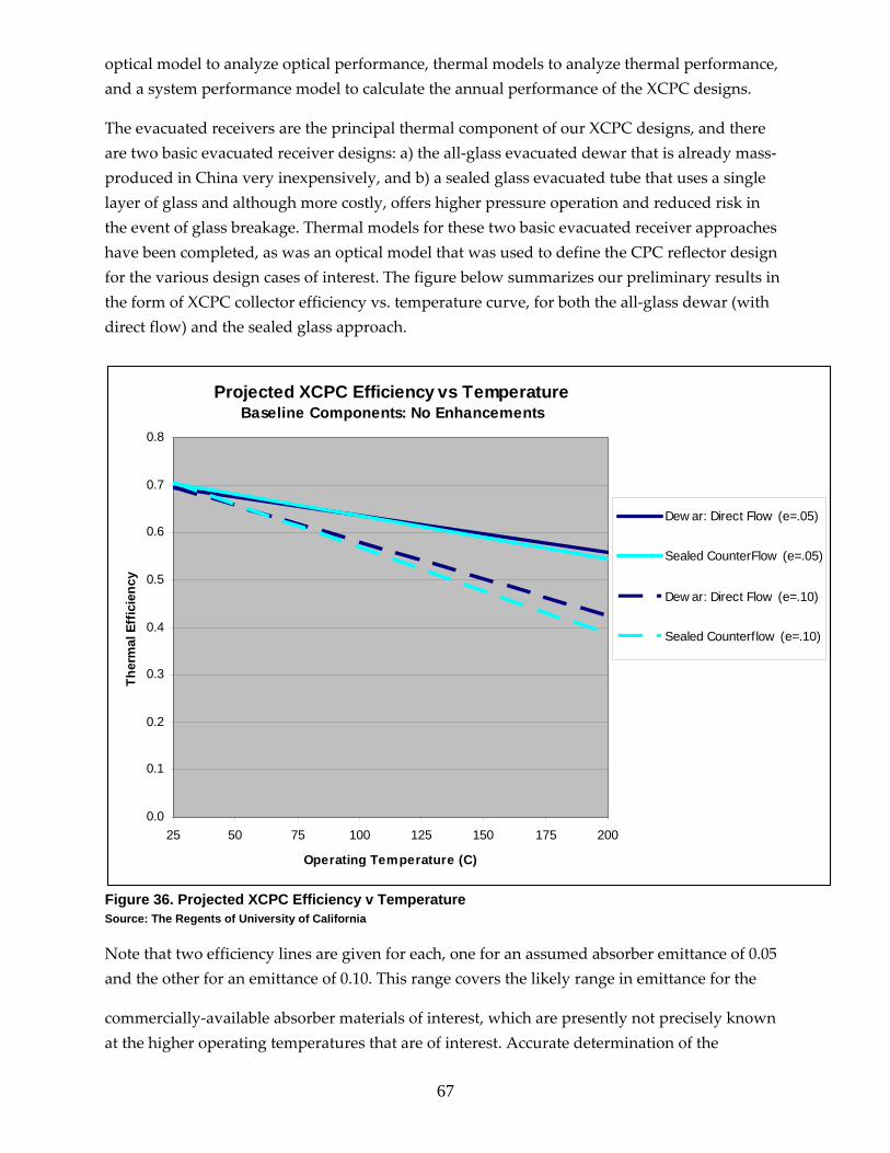
67
optical model to analyze optical performance, thermal models to analyze thermal performance, and a system performance model to calculate the annual performance of the XCPC designs.
The evacuated receivers are the principal thermal component of our XCPC designs, and there are two basic evacuated receiver designs: a) the all‐glass evacuated dewar that is already mass‐produced in China very inexpensively, and b) a sealed glass evacuated tube that uses a single layer of glass and although more costly, offers higher pressure operation and reduced risk in the event of glass breakage. Thermal models for these two basic evacuated receiver approaches have been completed, as was an optical model that was used to define the CPC reflector design for the various design cases of interest. The figure below summarizes our preliminary results in the form of XCPC collector efficiency vs. temperature curve, for both the all‐glass dewar (with direct flow) and the sealed glass approach.
Figure 36. Projected XCPC Efficiency v Temperature Source: The Regents of University of California
Note that two efficiency lines are given for each, one for an assumed absorber emittance of 0.05 and the other for an emittance of 0.10. This range covers the likely range in emittance for the
commercially‐available absorber materials of interest, which are presently not precisely known at the higher operating temperatures that are of interest. Accurate determination of the
Projected XCPC Efficiency vs TemperatureBaseline Components: No Enhancements
0.0
0.1
0.2
0.3
0.4
0.5
0.6
0.7
0.8
25 50 75 100 125 150 175 200
Operating Temperature (C)
Ther
mal
Eff
icie
ncy
Dew ar: Direct Flow (e=.05)
Sealed CounterFlow (e=.05)
Dew ar: Direct Flow (e=.10)
Sealed Counterflow (e=.10)

68
emittance of absorber selective surfaces awaits laboratory testing, and is part of Task 6 “Detailed Component Characterization”.
Note that, depending on the emittance of the selective coatings that are found, we are expecting to be very near our design point goal of 50% efficiency at 200oC. If the emittance values are as low as 0.05, we expect to be able to achieve thermal efficiencies that are slightly above our 50% goal. If the emittance values are 0.10, we expect to be closer to 40% in thermal efficiency at 200oC. Recall also that these designs are based on using standard off‐the‐shelf components, and do include the potential performance enhancements that will be evaluated in Task 10. The use of improved reflective materials, anti‐reflective coatings, and improved absorber coatings, for example, will boost operating these efficiencies.
Optical Analysis
For all three conceptual designs, the shape of the non‐imaging external reflectors was designed so that all sunlight impinging on the aperture plane of the collector within a 34° angular acceptance angle is redirected onto the absorber. The concentration factor, the optical efficiency and the incidence angle modifiers were calculated using raytracing analysis. Optical modeling software “TracePro” was used.
Figure 37. All-glass dewars – direct flow and all-glass dewar filled with thermal fluid - indirect flow Source: The Regents of University of California
The refractive index of the glass dewar was assumed to be 1.47 with a transmittance of 0.90. Each air/glass interface results in about a 4% reflection loss, and since there are two such interfaces the reflectance loss totals about 8%. The other 2% is due to absorption loss within the borosilicate glass.
The all glass dewar was assumed to have the following dimensions, consistent with the size of the most popular dewar that is mass‐produced in China.

69
Diameter of outer dewar wall: 58mm
Diameter of inner dewar wall: 47mm
The vacuum surface of the inner dewar wall was assumed to be coated with a selective coating with a 92% absorptance of the solar spectrum at normal incidence. The absorptance of selective coatings is known to depend upon incidence angle, and we accounted for this variation using Figure 38.
Figure 38. Variation of selective coating absorptance with incidence angle Source: The Regents of University of California
The external reflector was assumed to be of silver with a reflectivity of 90%, consistent with the use of Alanod’s best commercially available enhanced aluminum reflective material. The dimensions and the shape of the reflector are depicted in Fig. 39.

70
Figure 39. Shape of XCPC reflector for all-glass dewars Source: The Regents of University of California
The raytracing analysis yielded an average optical efficiency of 66.5% (averaged over all incidence angles smaller than the acceptance angle, i.e. between 0 and 34 degrees). The dependence of the optical efficiency on the incidence angle, the so‐called incidence angle modifier (IAM), is depicted in Fig. 40.
Figure 40. Incidence Angle Modifier (IAM) for 58mm OD dewars Source: The Regents of University of California
Metal absorber with glass‐to‐metal seal:
The refractive index of the evacuated glass tube was assumed to be 1.47, again consistent with the normal 90% transmittance of borosilicate glass tubing. The evacuated glass tube is assumed to have the following dimensions, based on information provided by Beijing Eurocon Solar.
Diameter of outer tube wall: 65 mm

71
Diameter of inner tube wall: 61.8 mm
The metal absorber was assumed to be a thin cylindrical copper fin of 56 mm in diameter with a selective coating of 92%, and the variation with incidence angle depicted in Figure 38.
The external reflector was assumed to be of silver with a reflectivity of 90%, as with the previous design, based on the use of Alanod. The dimensions of the reflector are depicted in Figure 41.
Figure 41. Incidence Angle Modifier (IAM) for design using absorber with glass-to-metal seal Source: The Regents of University of California
The raytracing analysis yielded an average optical efficiency of 67.5% (averaged over all incidence angles smaller than the acceptance angle, i.e. between 0 and 34 degrees). The dependence of the optical efficiency on the incidence angle, the so‐called incidence angle modifier (IAM), is depicted in Figure 41
Thermal Analysis
We developed thermal models (one for each of the basic conceptual designs) that describe the transfer of the heat flux from the concentrating optical system to the working fluid in the absorber tube of the XCPC. When the concentrated sunlight reaches the absorber tube, convective, conductive and radiant heat transfer mechanisms occur in the different interfaces that comprise the absorber tube. The developed model evaluates the direction and magnitude of heat transfer mechanisms associated with the evacuated tubes, and solves for the net flow of heat to/from the various materials and surfaces.
The thermal models are based on the application of Energy Conservation Laws for all the surfaces and materials that dictate the thermal performance if the collector (selective surface absorptance, selective surface emittance, material thermal conductivity, glass absorptance, and

72
various convective heat transfer coefficients). We applied the energy and mass conservation laws to all identified control volumes and obtained a set of equations describing the thermal performance of the system. More details are included in the appendix to this report. The equations are solved using the EES Program (Engineering Equation Solver Program), which uses an iterative mathematical technique to derive the solution.
The most important result of the model is the net heat loss from the evacuated tube for various operating temperatures and irradiance levels.
Figure 42. Sketch of all-glass dewar tube (cross-section) Source: The Regents of University of California
Thermal analysis of this design is based on consideration of the energy transfers noted below.
1. The external glass volume that is exposed to the ambient and to a uniform solar radiation flux from the outer side. This glass volume encloses the absorber layer on the inner side.
2. The internal glass volume that is exposed on the outer surface to a uniform solar radiation flux and to the external glass cover. This glass volume encloses the working fluid on the inner side.
3. The circulating working fluid enclosed by the internal glass, including the counter‐flowing fluid inside/outside the copper tube.

73
Figure 43. Sketch of all-glass dewar tube (side cross-section) Source: The Regents of University of California
The heat loss coefficient was determined to be 0.776 W/m2‐C for an assumed absorber emittance of 0.05, using the value listed by the manufacturer at a temperature of 100 C. At higher temperatures the emittance will increase, but the exact amount is unknown at present. We estimate that it will increase to no more than 0.10. At this higher emittance, the heat loss coefficient was determined to be1.36 W/m2‐C. Both of these heat loss coefficients assume a concentration ration (CR) of 1.8, the ratio between the aperture area of the CPC reflector divided by the circumference of the absorber
Figure 44. Metal absorber with glass-to-metal seal Source: The Regents of University of California
74
The team identified three relevant control volumes:
1. The external glass volume that is exposed to the ambient and to a uniform solar radiation flux from the outer side. This glass volume encloses the metallic absorber fin on the inner side.
2. The cylindrical copper fin absorber with the selective coating. The fin is welded to a metal counter flow tube.
3. The circulating working fluid enclosed by the metal counter flow tube. The heat loss coefficient was determined to be 0.919 W/m2‐C for an assumed absorber emittance of 0.05, using the value listed by the manufacturer at a temperature of 100 C. At higher temperatures the emittance will increase, but the exact amount is unknown at present. We estimate that it will increase to no more than 0.10. At this higher emittance, the heat loss coefficient was determined to be 1.83 W/m2‐C. Both of these heat loss coefficients assume a concentration ration (CR) of 1.8, the ratio between the aperture area of the CPC reflector divided by the circumference of the absorber. Annual System Performance Analysis
The annual performance tool f‐Chart has been determined to include all the necessary characteristics to provide an accurate means of determining the annual performance of the various XCPC designs. F‐Chart www.fchart.com allows for user input of optical efficiencies (at normal incidence), incidence angle modifiers (as determined by our optical raytrace model), and heat loss coefficients (as determined by the thermal models). Importantly for our purposes, f‐chart includes algorithms for performance analysis of CPC collectors, along with traditional flat plate collectors and evacuated tube collectors. Hence, rather than developing an entirely new annual performance model, f‐chart has been purchased. Weather data for hundreds of North American locations, the 16 California climate zones and numerous other locations are included with the program to estimate the long‐term average performance of:
• Domestic Water Heating Systems • Water Storage Space and Domestic Water Heating Systems • Active Collection with Building Storage Space Heating Systems • General Solar Heating Systems (e.g., process heating systems)
An example of the inputs (and descriptions of each) for the CPC collector are shown as follows:

75
SI units can also be used.

76

77
Figure 45. Example of inputs for CPC collector Source: The Regents of University of California

78
Appendix – Thermal Models for Task 5
Sealed Tube: Cylindrical Absorber, Counterflow
Figure 46 & 47. Transversal section and schematic of heat fluxes Source: The Regents of University of California
Incident solar radiation W/m2
Heat loss by air convection on glass external surface W/m2
Net heat transfer to/from the glass from/to the atmosphere (sky) due to glass emission/absorption of heat by radiation. Gray surfaces assumed.
W/m2
Net heat transfer to/from the glass from/to the absorber due to emission/absorption of heat (in the infrared according to their low blackbody temperature) by radiation to/from the absorber. Gray surfaces assumed
W/m2
Heat transferred by conduction to working fluid W/m2 Tg Temperature of glass cover K TA Temperature of absorber K T∞ Temperature of fluid K Tsky Temperature of atmosphere K ho Convection coefficient W/m2KGlass Properties
Solar radiation (300 – 2,700 nm) Infrared (>2,700 nm) αg = absorptivity ≈ 0.02 τg = transmissivity ≈ 0.90 ρg,S = reflectivity ≈ 0.08 ( αc + ρc + τc = 1 )
εg = emmisivity ≈ 0.92 αg,IR = absorptivity as a gray surface = εg ≈ 0.92 τg = transmissivity ≈ 0 ρg = reflectivity ≈ (1- αg,IR ) = (1- εg ) = 0.08
Glass
Absorber αA(τAGc )”
αgGc”
TSKY
Tg
Gc”
TA
q"cond
ρg,sGc”
ρA,S(τAGc )”
ρg,s[ρA,S(τAGc )]”τAGc”
q"rad: g↔sky
q"rad: A↔g
q"conv
T∞
ho
''cG"convq
"rad: g skyq ↔
"rad: A gq ↔
"condq

79
Pyrex 7740 type: Pyrex 7740 is a low expansion borosilicate glass. Pyrex glass is good for normal use temperature of 446 degrees F and maximum use temperature 914 degrees F. Pyrex can also be tempered to increase its mechanical strength, and is also heat shock resistant. Pyrex is resistant to acid and has high optical transmission over a wide wavelength range. The low alkali content of Pyrex makes this glass ideal for high‐purity laboratory applications.
Figure 48. Corning Pyrex 7740 Transmittance curve Source: The Regents of University of California
Absorber Properties (sputtered Al-AlN coating) Solar radiation (300 – 2,700 nm) Infrared (>2,700 nm)
αA = absorptivity ≈ 0.95 εA = emmisivity ≈ 0.05 τA = transmissivity = 0 ρA,S = (1-αA) = 0.05
εA = emmisivity ≈ 0.05 ρA = (1-αA) ≈ (1- εA ) = 0.95
Figure 49. Reflectance spectrum of a SS‐AlN cermet solar selective coating deposited using a commercial‐scale dc sputter coater. The
corresponding film has a solar absorptance of 0.95 and emisivity of 0.05 at 100oC. The
coating has the double cermet film structure AlN/SS‐AlN(LMVF)/SS‐
AlN(HMVF)/Al. Department of Physics, University of
Sidney Source: The Regents of University of California
Applying an energy balance to the glass interface:
Heat absorption by the glass in the solar spectrum.
Heat loss by air convection on glass external surface
Net heat loss of the glass due to glass emission of heat by radiation to the
"inq
"convq
"rad: g skyq ↔

80
Figure 50. Heat fluxes at glass interface Source: The Regents of University of California
atmosphere (sky)
Net heat absorption by the glass due to glass absorption of heat (in the infrared according to its low blackbody temperature) by radiation from the absorber.
(1)
(2) Where:
h0 = 2.8 + 3v (according to the empirical equation proposed by Watmuff for a flat plate collector)
v = wind speed (ms-1) (Since the view factor between the tube and the sky is 1)
Equation (2) is more useful if expressed as a heat rate [ W ] :
(3) Where: Ag = Area of glass tube = (πDg)L AA = Area of absorber = (πDA)L Applying an energy balance to the absorber:
Net heat absorption by the selective coating of the transmitted solar radiation plus the multiple absorber-glass reflections of transmitted solar radiation.
"rad: A gq ↔
'' '' '' ''in rad: A g conv rad: g skyq + q - [ q + q ] 0↔ ↔ =
α σ σ'' 4 4 4 4g c rad: A g A g 0 g rad: g sky g skyG + h (T -T ) - h (T -T ) - h (T -T ) 0↔ ∞ ↔ =
εε ε
rad: A gg g
A g A
1h1- r1 +
r
↔ =⎛ ⎞⎜ ⎟⎝ ⎠
εrad: g sky gh = ↔
α σ ε σ'' 4 4 4 4g g c A rad: A g A g g 0 g g g g skyA ( G ) + A [ h (T -T ) ] - A [ h (T -T ) ] - A [ (T -T ) ] 0↔ ∞ =
"absorbedq

81
Figure 51. Heat fluxes at absorber interface Source: The Regents of University of California
Net heat loss of the selective coating due to selective coating emission/absorption of heat (in the infrared according to its low blackbody temperature) by radiation to/from the glass.
Heat conducted per unit area to working fluid.
(4)
(5)
Equation (4) is more useful if expressed as a heat rate [ W ] :
(6)
Where: AA = Area of absorber = (πDA)L
DA = 56 mm Do = 10 mm to = 1 mm
tA = 0.3 mm
Figure 52. Heat fluxes at absorber / heat exchanger Source: The Regents of University of California
"rad: A gq ↔
"condq
'' '' ''absorbed rad: A g condq - q - q 0↔ =
α τα ρ
A g '' ''c rad: A g A g cond
A g,sG - h (T -T ) - q 0
1 (1 ) ↔ =− −
α τα ρ
A g '' ''A c A rad: A g A g A cond
A g,sA G - A [ h (T -T ) ] - A q 0
1 (1 ) ↔
⎛ ⎞=⎜ ⎟⎜ ⎟− −⎝ ⎠
π ADR=2
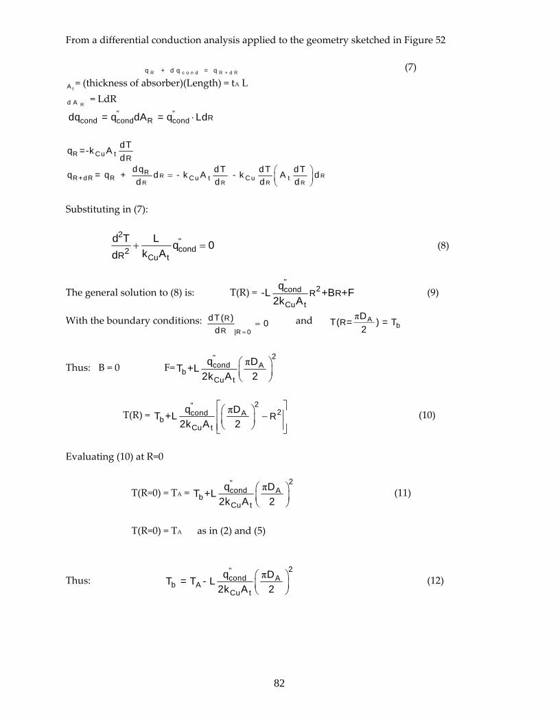
82
From a differential conduction analysis applied to the geometry sketched in Figure 52
(7) = (thickness of absorber)(Length) = tA L = LdR
Substituting in (7):
(8)
The general solution to (8) is: T(R) = (9)
With the boundary conditions: and
Thus: B = 0 F=
T(R) = (10)
Evaluating (10) at R=0
T(R=0) = TA = (11)
T(R=0) = TA as in (2) and (5)
Thus: (12)
R c o n d R + d Rq + d q = q
tA
Rd A
" " Rcond cond R conddq = q dA = q Ld⋅
R Cu t R
dTq =-k Ad
R RR R R R
RR +dR R C u t C u t
dq dT dT dTq = q + d - k A - k A dd d d d
⎛ ⎞= ⎜ ⎟⎝ ⎠
2"cond2
Cu tR
d T L q 0k Ad
+ =
"2cond
Cu tR R
q-L +B +F2k A
|R 0
R
R
dT( ) 0d =
=π A
bRDT( = ) = T2
π 2"cond A
bCu t
q DT +L2k A 2
⎛ ⎞⎜ ⎟⎝ ⎠
π 2"2cond A
bCu t
Rq DT +L
2k A 2
⎡ ⎤⎛ ⎞⎢ ⎥−⎜ ⎟⎝ ⎠⎢ ⎥⎣ ⎦
π 2"cond A
bCu t
q DT +L2k A 2
⎛ ⎞⎜ ⎟⎝ ⎠
π 2"cond A
b ACu t
q DT = T - L2k A 2
⎛ ⎞⎜ ⎟⎝ ⎠

83
From the thermal circuit illustrated in Figure 53:
(13)
Figure 53. Thermal Circuit Source: The Regents of University of California
From the solution of the heat exchanger:
(13)
Where ΔT = Tout ‐ Tin (14)
SUMMARY: Equations derived for the Absorber – Heat exchanger system under the following assumptions:
• Steady state
• Heat exchange by radiation between the absorber, glass and ambient is treated as a gray
surface phenomena in the IR region.
• The flux in the absorber is considered to have a uniform distribution in the whole
surface.
• Heat exchange by radiation between the internal wall of the absorber and the external
wall of the heat exchanger is neglected.
• No temperature drop across the glass.
(A)
(B)
π π
b outcond
o o 0
0 in Cu
T -Tq = ln[(D +2t )/D ]1 +D Lh Lk
π
0 00
Cu
D 2tln D2 Lk
+⎛ ⎞⎜ ⎟⎝ ⎠
π 0 in
1 D Lh
cond
o p,o
qΔT = m c&
α σ ε σ'' 4 4 4 4g g c A rad: A g A g g 0 g g g g skyA ( G ) + A [ h (T -T ) ] - A [ h (T -T ) ] - A [ (T -T ) ] 0↔ ∞ =
α τα ρ
A g '' ''A c A rad: A g A g A cond
A g,sA G - A [ h (T -T ) ] - A q 0
1 (1 ) ↔
⎛ ⎞=⎜ ⎟⎜ ⎟− −⎝ ⎠

84
(C)
(D)
(E)
Tout = ΔT + Tin (F)
RESULTS The solutions to equations A to F were obtained with the use of the EES software for a constant flow rate of 1.5 liter/min and two different conditions: A: Constant irradiation, = 1000 W/m2 (which translates in a heat rate of = 326.7 W )
Different input temperatures of fluid, Tin Table 1 Figure 52 B: Constant input temperatures of fluid, Tin Different irradiation rates, Gc Table 13 Table 14 Table 15 Figure 10 Figure 11 Figure 12
π π
b outcond
o o 0
0 in Cu
T -Tq = ln[(D +2t )/D ]1 +D Lh Lk
π 2"cond A
b ACu t
q DT = T - L2k A 2
⎛ ⎞⎜ ⎟⎝ ⎠
cond
po
qΔTm c
=&
''cG ''
g cA G

85
Table 12. Variation of output temperature of fluid when irradiation is kept constant at Gc = 326.7 W
Source: The Regents of University of California
Where the total efficiency is defined as:
Figure 53. Output temperature of fluid when irradiation is kept constant and while fluid input temperature varies according to table 1 Source: The Regents of University of California
condtotal "
g c
qEff = A G

86
Figure 54. Differences in Temperature: Absorber – Input and Output - Input Source: The Regents of University of California
CONDITION B: Constant input temperatures of fluid, Tin Table 13. Variation of output temperature of fluid when the input temperature is kept constant at Tin=400 K Source: The Regents of University of California
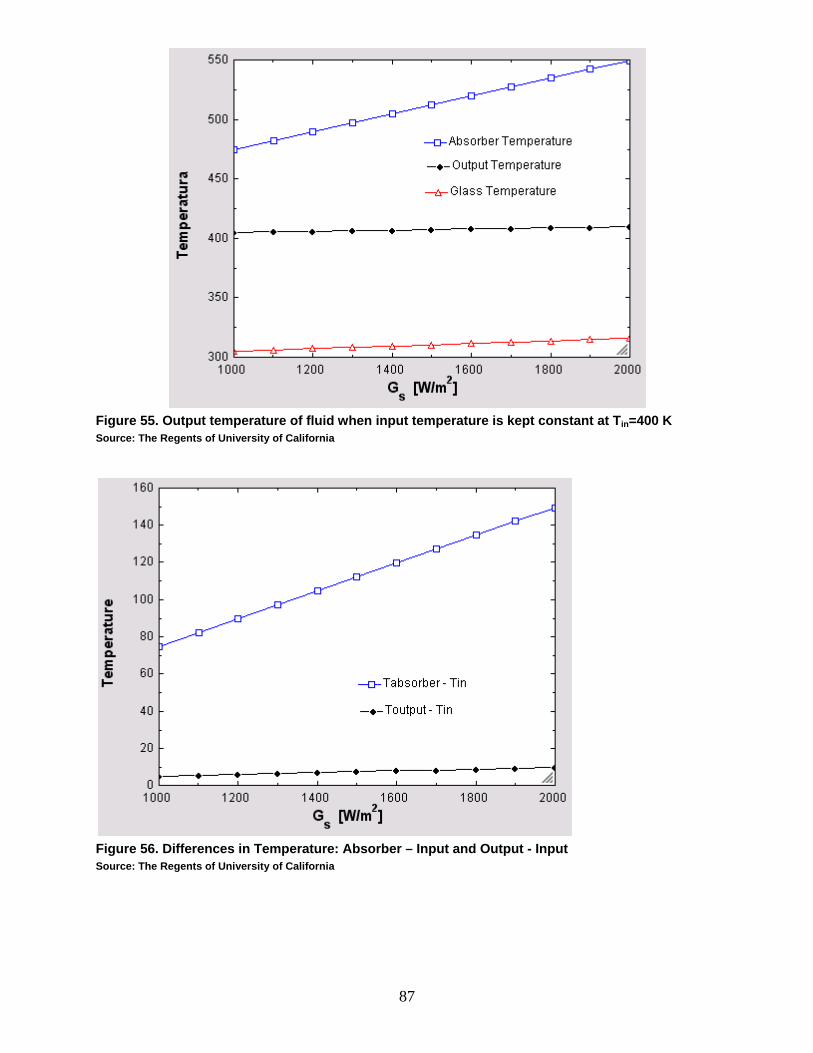
87
Figure 55. Output temperature of fluid when input temperature is kept constant at Tin=400 K Source: The Regents of University of California
Figure 56. Differences in Temperature: Absorber – Input and Output - Input Source: The Regents of University of California

88
Table 14. Variation of output temperature of fluid when the input temperature is kept constant at Tin=473 K Source: The Regents of University of California
Figure 57. Output temperature of fluid when input temperature is kept constant at Tin=473 K Source: The Regents of University of California

89
Considering thermal resistance of absorber
Figure 58. Output temperature of fluid when input temperature is kept constant at Tin=473 K Source: The Regents of University of California
Neglecting thermal resistance of absorber
Figure 59. Differences in Temperature: Absorber – Input and Output – Input Source: The Regents of University of California

90

91
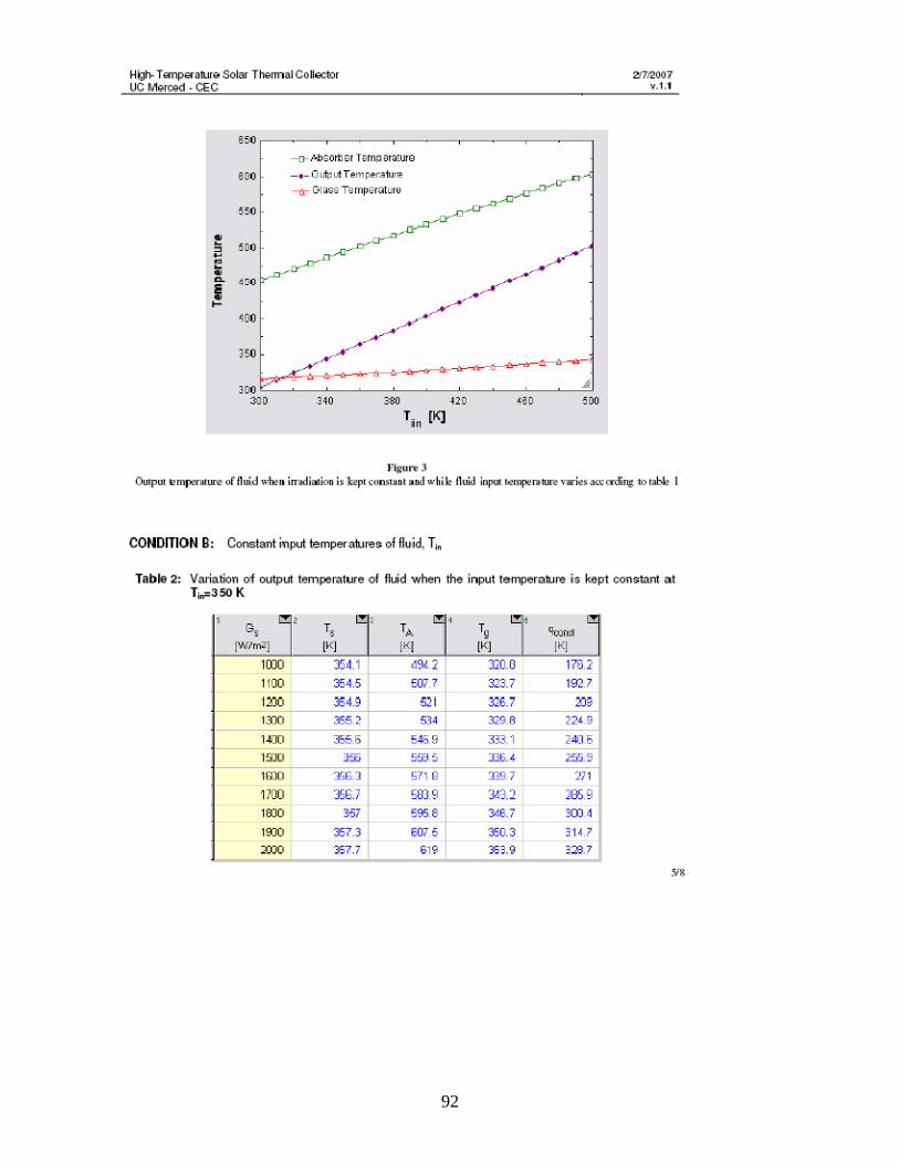
92

93

94

95
2.5. Task 6 In Task 6, the Contractor has determined the important properties of the existing off‐the‐shelf components that are being considered for the XCPC. This report is a summary of these component properties. The analyzed components are:
• Reflector • Glass tube • Selective coating of absorber • Heat pipe
Reflector Properties The three primary types of reflectors suitable for solar concentrators are: silvered glass, polymeric films, and polished/enhanced aluminum sheet. Unfortunately, solar reflector materials have long been a “weak spot” of solar technology, and there are very few commercially‐available reflector materials for use in solar concentrators. Long‐term outdoor use requires good outdoor weather ability, ultra‐violet stability, and good mechanical stability and durability under the extremes of the outdoor environment. Silvered‐glass reflectors offer high reflectance and good outdoor weather ability, but they are quite heavy and fragile. Also, to create the CPC‐shaped reflectors that we need for the XCPC will necessitate a significant R&D effort, akin to the major effort that SolFocus is engaged in for their concentrating photovoltaic system that is under development. Since the Task 6 effort is aimed toward existing off‐the shelf components, we have not considered the silvered glass approach here.

96
Metalized polymer films are another type of reflector, and the 3M Company offered several types of metalized films for solar use for many years. 3M manufactured an aluminized film, but it had a reflectance in the mid‐80’s, which was deemed to be too low and so this film was discontinued. A silvered acrylic film, called ECP‐305+, was also made by 3M. But it suffered from “tunneling” problems (essentially, delaminating the acrylic from the silver layer) which ultimately results in 3M’s discontinuation of this film too. A relatively recent silvered film has been developed by NREL and ReflecTech, and we consider this alternative in our Task 10 work, which includes consideration of some advanced components and possibilities for performance enhancement with further component development. Polished aluminum reflectors are generally judged to be the most commercially‐available for outdoor solar use. And while polished aluminum is known to lose significant specular reflectance after just 2 to 3 years of outdoor use, Alanod1 (a German‐based company) has made a great deal of technical progress in advancing and improving this approach. Alanod has developed specialized coating techniques that increase the reflectance of their aluminum‐based reflective materials, as well as increase outdoor weatherability. Alanod has two commercially‐ready reflective materials for outdoor solar energy utilization: Alanod MiroSun and Alanod 4270 KKSP. Both are aluminum based reflectors, and samples of these materials were supplied to NREL for optical measurements. The measured hemispherical reflectance vs. wavelength values is shown below.
Fiure 60. Spectral reflectance of Alanod Reflective Surfaces Source: The Regents of University of California
1 http://www.alanod.com/opencms/sites/alanod.de/en/miro/MIRO-SOLAR/mirosun.html
Spectral Reflectance of Alanod Reflective Surfaces
80
82
84
86
88
90
92
94
96
98
100
400 800 1200 1600 2000
Wavelength (nm)
Hem
isph
eric
al R
efle
ctan
ce (%
) _
Alanod 4270 KKSPAlanod Miro Sun

97
Weighting the reflectance values by an airmass‐1.5 solar spectrum allows determination of the overall hemispherical reflectance for solar thermal applications, since the entire solar spectrum provides useful energy for thermal conversion. The solar‐weighted hemispherical reflectance of Alanod Miro Sun is 91.9%. The solar‐weighted hemispherical reflectance of Alanod 4270 KKSP is 91.5%. Hemispherical reflectance includes all reflected light from the sample, regardless of its reflected direction.
Another common way to characterize reflective surfaces is to measure specular reflectance, which excludes reflected light that is scattered, that is, reflected outside a specified acceptance cone angle. The Devices and Services portable specular reflectometer Model 15R provides this measurement, but for a specific wavelength of 660 nm. This instrument was used to measure specular reflectance of both Alanod reflector materials, with the largest acceptance angle (46 milliradians) available on the Model 15R. Alanod MiroSun measured 86%, and the 4270 KKSP measured 90.0%. There is a significant difference between the specular reflectance values at 660 nm and the hemispherical reflectance (also taken at 660 nm), indicating that there is a significant amount of scattering. Given the high acceptance angles of the CPCs, we expect that performance will be more closely governed by hemispherical reflectance than specular reflectance, but will be somewhere in between. To be conservative, in our modeling efforts to date we have assumed a reflectance value of 90%.
The specularity of reflective materials is known to sometimes be affected by material forming operations (such as bending, roll‐forming, etc.) since these operations can sometimes alter the front portions of the reflective material. To determine whether this might be the case with Alanod, for the radii needed for our CPC, a virgin piece of flat Alanod 4270 KKSP was measured with the Devices and Services portable specular reflectometer, then formed/rolled to a radius of 1.12 inches (28 mm) as shown in the left‐most photo below.
Figure 61: Measuring radius Figure 62: Reflectivity measurements of Alanod Source: The Regents of University of California Source: The Regents of University of California

98
The formed sheet was then flattened, and measurements were obtained again with the D&S specular reflectometer2, as shown in the right‐most photo above. These measurements were within 0.1% of the original values, indicating that specularity loss is not anticipated to be an issue for the amount of roll‐forming required to form the CPC profiles.
Glass Transmittance
The commercially available evacuated tubes that are mass‐produced in China use borosilicate glass. Borosilicate glass is a high quality glass with low thermal expansion and excellent solar transmittance. Solar energy absorption within the glass is very small; the optical loss of borosilicate glass is dominated by reflection losses (Fresnel losses) due to the higher index of refraction of glass compared to air. As light passes through a glass cylinder (e.g. a glass dewar) to the absorber surface within it, the light encounters two interfaces: one at the outer surface of the glass and one at the inner surface of the glass. Each interface yields a loss of about 4%, so the total reflectance loss is about 8%.
The transmittance of a typical borosilicate glass (Corning 7740) sample is shown below, and yields a solar‐y
Figure 63. Corning Pyrez 7740 Transmittance Source: The Regents of University of California
To verify that the glass used in the Chinese‐manufactured evacuated tubes is of the same high quality as noted above, samples were taken from a Chinese‐manufactured evacuated tube (i.e. the standard dewars we contemplate using in certain of our XCPC designs) and tested at NREL
2 http://www.devicesandservices.com/

99
by Cheryl Kennedy for transmittance with their Perkin‐Elmer spectrophotometer. The instrument is pictured below to the left, and a close up of the glass sample, mounted in the instrument, as shown on the next page:
Figure 64. Perkin-Elmer spectrophotometer Figure 65. Perkin-Elmer spectrophotometer Source: The Regents of University of California Source: The Regents of University of California
The measured transmittance vs. wavelength is shown below.
Figure 66. Borosilicate Glass Tube Transmittance Source: The Regents of University of California
The solar‐weighted transmittance was found to be 91.7%, a bit higher than anticipated and a good indication that the glass is indeed of high quality.
Borosilicate Glass Tube Transmittancesolar-weighted value = 91.7%
Tested at NREL on Feb. 21 2007
0102030405060708090
100
250 500 750 1000 1250 1500 1750 2000 2250 2500
wavelength (nm)
Hem
isph
eric
al
Tran
smitt
ance

100
Figure 67. Selective coating properties
Source: The Regents of University of California
Selective Coatings
The two performance‐related properties of the selective coatings are absorptance and emittance. Although there are some limited absorptance and emittance values available from product suppliers, we have taken steps to determine these two properties through independent testing.
Most of the commercially available evacuated tubes that are mass‐produced in China use an aluminum nitride vacuum sputtered coating that provides for selective properties. With the term “selective” we mean spectrally selective, an absorber that has different spectral reflectance at different wavelengths. We desire that the reflectance of the coating over the solar spectrum is very low, while the reflectance of the coating over most of the infra‐red spectrum is very high. An example of a very high quality highly‐selective Mo‐Al2O3‐on‐stainless coating is illustrated in the figure below as the heavier solid blue line. Note that the reflectance increases sharply just above the wavelengths of the solar spectrum (the solid red line). Note also that the blackbody spectrum for temperatures of 100oC, 300oC and 400oC are also indicted on the figure. Since the blackbody spectrum increasingly extends into the lower wavelength regions as the temperature increases, it is clear that selective surfaces can be expected to have increased emittance as temperatures increase. There is another factor at work here also, which can further increase the emittance of the selective coating as temperature increases. The reflectance vs. wavelength relationship of surfaces (and selective coatings) can change, depending on temperature. The heavy blue solid line reflectance values are typically obtained using a spectrophotometer, with the sample at

101
room temperature. But at higher temperatures, the reflectance values can be different. To account for this change, and be sure that the proper emittance is known (especially if thermal models are being used for performance prediction) it is best to measure the selective coating reflectance values at the higher temperatures of interest. Since the selective coating emittance is a key determinant of the performance of our XCPC collectors, samples have been measured at room temperature and 200oC, as part of this Task 6 work effort. Few laboratories have the capability to measure emittance at 200oC. NREL presently does not, for example, but they referred us to Surface Optics Corporation (SOC) in San Diego. SOC measured the optical properties of selective coating samples that we provided to them from:
a) three commercially available Chinese dewars manufacturers (Paradigma, Tsinghua, and SunRain),
b) a commercially‐available selective foil (TiNOX) that can be used within our sealed‐glass design, and c) a custom‐produced vacuum‐deposited selective foil manufactured in China by Eurocon, the vendor that has manufactured our sealed‐glass prototype tubes.
The emittance results obtained by SOC for these various selective coatings are provided below in Table 1, along with the solar‐weighted absorptance of the coatings, another key optical characteristic that is of primary importance. A coatings solar‐weighted absorptance is the fraction of the solar spectrum that will be absorbed by the coating.
Also, to gain a full understanding of absorptance, we need to determine the variation of absorptance with incidence angle. This can have a significant impact on performance. A typical illustration of this affect is shown below. (We have used this figure for our performance estimates.)
Solar‐Wt Emittance Emittance Coating
Chinese all‐glass dewars Absorptance @ 27C @ 200C Substrate
Paradigma 0.883 0.1 0.15 glass
Tsinghua 0.923 0.05 0.074 glass
SunRain 0.913 0.047 0.088 glass
Metal Foils for Sealed Glass Tubes
TiNOX 0.958 0.035 0.158 copper
Eurocon 0.902 0.05 0.064 aluminum
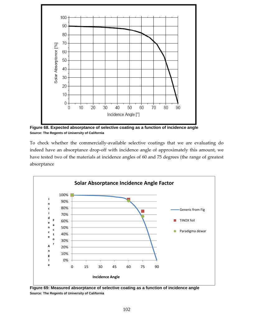
102
Figure 68. Expected absorptance of selective coating as a function of incidence angle Source: The Regents of University of California
To check whether the commercially‐available selective coatings that we are evaluating do indeed have an absorptance drop‐off with incidence angle of approximately this amount, we have tested two of the materials at incidence angles of 60 and 75 degrees (the range of greatest absorptance
Figure 69: Measured absorptance of selective coating as a function of incidence angle Source: The Regents of University of California
0%
10%
20%
30%
40%
50%
60%
70%
80%
90%
100%
0 15 30 45 60 75 90
Incidence
Angle
Factor
Incidence Angle
Solar Absorptance Incidence Angle Factor
Generic from Fig
TiNOX foil
Paradigma dewar

103
decrease) and compared these values with their normal‐incidence absorptance values. The data points obtained (for the TiNOX foil and the Paradigma dewar) are plotted onto the generic figure shown earlier. Note that the values are in quite good agreement with what had been expected.
Heat Pipes
The approximate capacity of the Chinese heat pipes that we consider using for the XCPC has been estimated by United Technologies Research Center using simple modeling techniques from first principles. It is to be noted that the analysis was done based on the external geometrical dimensions and the data provided by the manufacturer about internal construction and contents of the tube.
Background
Thermosyphons and heat pipes are devices that transport heat from one location to another (or one fluid stream to another) by using a cyclic process of vaporization and condensation of a charge (working fluid) inside a sealed tube. Heat is supplied to the evaporator (or hot end) of the tube which conducts across the tube wall and heats the working fluid inside which upon reaching its vaporizing temperature evaporates to the center of the tube and travels towards the cold end (condenser) of the tube. Typically the cold end is cooled by external means, whereby the vapor inside the tube reaching the cold end condenses, giving up the latent heat of vaporization. The condensed fluid inside the tube then must return back to the evaporator end of heat pipe, so that the cycle can continue. In heat pipes this return of the condensed fluid back to the evaporator end is achieved by intricate wick structures through which the liquid can travel using surface tension. In thermosyphons there are no wicks and hence return of fluid to evaporator is solely aided by gravity. As such in thermosyphons the devices must be so installed that the condenser is at an elevated level with respect to the evaporator. In this report, however, the terms “heat pipes” and “thermosyphons” will be used interchangeably unless a distinction needs to be made.
In both devices, however, since the heat transfer occurs by means of evaporation/ condensation of a fluid at or near its saturated state, there is very little temperature gradient between the hot and cold ends (in other words there is very little difference in “quality” of the heat as it travels from hot to cold end, unlike solid metal conductors). Also, since latent heats of vaporization of the commonly used fluids are large, a relatively high rate of heat transfer is possible, depending on the mass flow rate of the fluid inside. Furthermore, the operating temperature of a heat pipe is fairly constant at its design temperature, since the saturation temperature of any fluid is constant at a given pressure and once manufactured there is no way to change the pressure inside sealed heat pipes. Heat Transfer Limitations of a Heat Pipe
The amount of thermal energy that a heat pipe can transport from its hot end to its cold end can be limited by three major ways:

104
1. Maximum heat that can be radially transferred from the hot external source to the working fluid inside – Evaporator Limit – which is a function of the tube wall properties and geometry, surface area of heat pipe at the evaporator section, and temperature difference between source and the operating temperature of the heat pipe. 2. Axial heat transport limit of the heat pipe – Axial Heat Flux Limit – which can be due to Capillary Limit, Boiling Limit, Entrainment Limit, Sonic Limit and some other limiting criteria, some of which will be discussed in detail below. 3. Maximum heat that can be radially transferred from the working fluid inside at the cold end to the external sink – Condenser Limit ‐ which is a function of the tube wall properties and geometry, surface area of heat pipe at the condenser section, and temperature difference between sink and the operating temperature of the heat pipe. In this analysis, the Evaporator Limit of the heat pipe is not evaluated. The work here focuses on estimating the Axial Heat Flux Limit and the Condenser Limit. Assumptions
The purchased Chinese off‐the‐shelf devices (from Beijing Eurocon Solar Energy Tech. Co. Ltd.) are clearly thermosyphons, since they do not have any internal wick structure. The charge inside is a proprietary mixture which is 80% by volume water and water is the only fluid that participates in heat transfer. It is assumed that while the pipe is designed for 80 – 100 C operation, it can be operated safely at a much elevated temperature of 200 C. The intent of this analysis is to estimate the performance of the device as it operates at 200 C. Fig.1 shows the heat pipes and the known key physical attributes.
Calculation of Axial Heat Flux
Axial transport of heat in a thermosyphon can be limited by a number of physical phenomena like attainment of sonic velocity in the heat pipe vapor, entrainment of the heat pipe liquid by its vapor or the onset of boiling in the heat pipe liquid. There are some other means of limiting the heat flux and Table 1 (Ref. 1) provides a list and a brief explanation. Based on our understanding of the operating procedures of these heat pipes, it is thought that only limits due to entrainment or vapor reaching sonic velocity are of relevance.

105
Figure 70. Beijing Eurocon Heat Pipe Geometry and Characteristics Source: The Regents of University of California
Sonic Limit
Sonic Velocity Limit is calculated based on the maximum allowable velocity of the vapor in the evaporating section of the heat pipe which cannot exceed the sonic velocity of vapor at the operating temperature of the heat pipe. Based on this limiting velocity, density of vapor and latent heat of vaporization, the maximum axial heat flux limit Qs (Eqn. 1) is calculated. The Sonic Limit is simply this axial heat flux multiplied by the available cross‐section for vapor flow.
Qs = …………………………….Eqn. 1
where � = Density of vapor,
V = Sonic velocity in evaporator
L = Latent heat of vaporization
= Gas Constant for steam
& FM = Momentum Correction Factor
Heat Pipe Dimensions
8 mm OD0.75 mm Wall Thickness24 mm Condenser Dia2 mm Condenser Wall Thickness2.1 m Long Axially
Heat Pipe Materials
No Internal W ickWall of 99.9% Cu (T2)Transport Fluid is 80% Water byVolume
Heat Pipe Orientation
Evaporator at bottom andCondenser on Top
Heat Pipe oriented at 45 deg tovertical
21
*)1(1Γ+
Γ++ FMVLρ

106
Calculation of Sonic Limit was performed at 100 C, 150 C, 200 C and 250 C and the results are shown in Table 15.
Table 15. Heat Pipe Heat Transport Limitations Source: The Regents of University of California
Entrainment Limit
Entrainment Limit is essentially due to the fact that water returning from the condenser is entrained in the vapor flowing towards the condenser and this water is lost from the evaporation process, thereby limiting the heat transfer rate. In a thermosyphon, this can happen due to two separate processes which can be interrelated. However, since an analysis that accounts for these two effects together can be very complicated, in this first order analysis the two phenomena are considered independently. The first of these effects is due to the vapor inertia force acting over the vapor space cross‐section, which can result in liquid drops being stripped by vapor and being carried back to condenser without getting a chance to evaporate. In this study, this entrainment limit is denoted as QE,vap. This vapor inertia force is countered by the stabilizing force of surface tension of the liquid, acting over the circumference of the vapor space, which prevents droplet formation. Typically, this competing nature of two forces is quantified in the Weber Number (We = �V2D/4�), where V is the velocity of the vapor, D is the vapor space diameter and � and � are explained below. For Weber Number more than 1, it is assumed that entrainment takes

107
place. After solving for the vapor velocity by setting Weber No to 1, the vapor‐based entrainment limit flux QE, vap is calculated according to Eqn. 2. In typical heat pipes with wicks, this is the only limit that is relevant. QE,vap = L* ………………………….……………..Eqn. 2
where = Momentum Factor = 2.2 for turbulent flow,
� = Density of vapor
������ ����������� = Surface tension of liquid water
An additional mechanism for entrainment should be investigated in the thermosyphons under consideration, since they are wickless and the liquid return is solely under the influence of gravity. In such a situation, the liquid “trickles” down the walls of the pipe from the condenser and the film thickness and velocity of flow are determined by well defined correlations that depend on the viscosity and the surface tension of the liquid. For films thicker than this limiting thickness, the water film will develop instabilities on the surface and break down into drops which can be entrained in the vapor flowing out of the evaporator. This entrainment limit, denoted by QE,liq, is also based on Weber Number being equal to or more than 1. However, the Weber No is defined as We = /2�, where �and V refer to liquid density and film velocity respectively and � is the thickness of the liquid film. The velocity of a liquid film falling under gravity is given by the well‐known Eqn. 3. Combining with the definition of Weber No and setting We to1, one can derive Eqn. 4 to calculate the liquid film thickness. This will lead to the calculation of liquid film velocity and hence the limiting rate of liquid return. The QE,liq can be calculated as the product of this liquid flow rate and the latent heat of vaporization of water as in Eqn.5. Vl = 2 ………………………………………Eqn. 3
and
� = …………………………………..…Eqn. 4
where � = Viscosity of water,
g = Acceleration due to gravity
& = the angle with the vertical
QE,liq = A*L* ………………………………….........Eqn. 5
Table 16 shows the calculated values of QE,vap and QE,liq for operating temperatures of 100 C, 150 C, 200 C and 250 C. For 200C, this limiting flux is 1.25 kW. Since the needed heat transport
DΩΠσρ2
Ω
δρ 2Vl lρ
δμ
θρ3cosgl
51
22
2
)cos(18
θσσμ
g
θ
ll Vρ
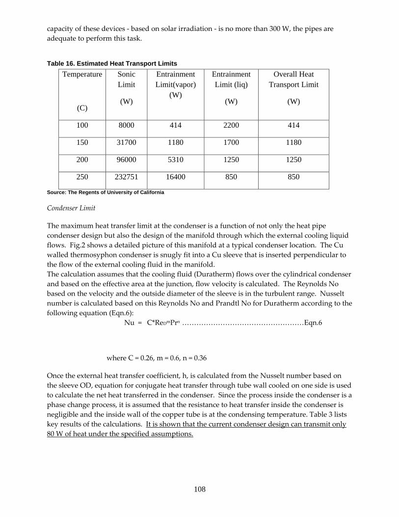
108
capacity of these devices ‐ based on solar irradiation ‐ is no more than 300 W, the pipes are adequate to perform this task.
Table 16. Estimated Heat Transport Limits Temperature
(C)
Sonic Limit
(W)
Entrainment Limit(vapor)
(W)
Entrainment Limit (liq)
(W)
Overall Heat Transport Limit
(W)
100 8000 414 2200 414
150 31700 1180 1700 1180
200 96000 5310 1250 1250
250 232751 16400 850 850
Source: The Regents of University of California
Condenser Limit
The maximum heat transfer limit at the condenser is a function of not only the heat pipe condenser design but also the design of the manifold through which the external cooling liquid flows. Fig.2 shows a detailed picture of this manifold at a typical condenser location. The Cu walled thermosyphon condenser is snugly fit into a Cu sleeve that is inserted perpendicular to the flow of the external cooling fluid in the manifold. The calculation assumes that the cooling fluid (Duratherm) flows over the cylindrical condenser and based on the effective area at the junction, flow velocity is calculated. The Reynolds No based on the velocity and the outside diameter of the sleeve is in the turbulent range. Nusselt number is calculated based on this Reynolds No and Prandtl No for Duratherm according to the following equation (Eqn.6):
Nu = C*ReDmPrn ……………………………………………Eqn.6
where C = 0.26, m = 0.6, n = 0.36
Once the external heat transfer coefficient, h, is calculated from the Nusselt number based on the sleeve OD, equation for conjugate heat transfer through tube wall cooled on one side is used to calculate the net heat transferred in the condenser. Since the process inside the condenser is a phase change process, it is assumed that the resistance to heat transfer inside the condenser is negligible and the inside wall of the copper tube is at the condensing temperature. Table 3 lists key results of the calculations. It is shown that the current condenser design can transmit only 80 W of heat under the specified assumptions.

109
Discussion
The above analysis clearly establishes the overall limits of the Beijing Eurocon thermosyphons at different operating conditions. Particularly at 200 C – the operating temperature of interest, the device transfers 80 W of heat, limited by the condenser performance. It is imperative that the condenser (and/or manifold) design be improved to be able to use them in solar applications, where the demand is to transfer 300 W per pipe. However, a few other issues are of concern too.
Figure 71. Manifold and Heat Pipe Arrangement Source: The Regents of University of California
2 m
m
A33 mm
B C
26 mm
D
Manifold Cooling Fluid
Manifold Condenser
2 m
m
A33 mm
B C
26 mm
D
2 m
m2
mm
A33 mm
B C
26 mm
D
A33 mm
B C
26 mm
D
Manifold Cooling Fluid
Manifold Condenser

110
Table 17: Condenser Side Heat Transfer Estimates Source: The Regents of University of California
Flow Rate of Duratherm
gpm 1
Prandtl No. 25.7
Effective Flow Area in Manifold
cm^2 9.67
Reynolds No 8700
Nusselt No 194
Heat Transfer Coefficient, h
W/m^2/K 1010
Temperature Difference Across
Condenser
C
30
Heat Transfer from Condenser
W 81
Firstly, it has been suggested that these pipes are originally designed to operate between 80 and 100 C and to transfer about 100 W (consistent with condenser design and Table 16 data). If they are operated at 200 C, then the vapor inside is operating at a superheated state. The pressure of superheated steam at 200 C is about 1.5 MPa. So one hopes that the tubes are strong enough to withstand this pressure for which they were not built. Secondly, the only way it will operate at 200 C is if the minimum temperature of the manifold fluid is 200 C. In the manifold, the thermosyphons are arranged in series and the first one in the series will encounter fluid returning from CHP heat exchanger at approximately 130° C (according to current design). It is United Technologies’ belief that the heat pipe will operate around this temperature rather than 200 C. The subsequent pipes in the same manifold will each operate at progressively higher temperature. But given the expected temperature rise of 30° C across the entire manifold, it is expected no heat pipe will operate above 160° C.
2.6. Task 7 As described in the XCPC Conceptual Design Report (Task 4), we formulated three competing conceptual level designs for the External Compound Parabolic Concentrator (XCPC) that were developed during the course of this project. The performance goal was a collector efficiency of at least 50 percent at a temperature of 400ºF, and a cost goal (uninstalled) of $10 per square foot,

111
or lower. Each of the formulated designs consists of an assembly of stationary evacuated tube absorbers with external non‐imaging reflectors. The three competing design concepts that were formulated are:
1. All glass dewar: Direct Flow
2. All glass dewar filled with thermal fluid: Indirect Flow
1. Metal absorber with glass‐to‐metal seal
Each of these designs was considered, one by one, and is presented with the expected performance for. Design #1 ‐ All glass dewar: Direct Flow The heat transport fluid flows directly inside the all‐glass dewar – hence we use the term “direct flow”. The design uses very inexpensive all‐glass dewar solar thermal absorbers that are mass produced in China. The dewars are cylindrical borosilicate glass bottles with an evacuated annulus between the two glass walls. A crossectional diagram of the dewar is shown in Figure 72 The vacuum surface of the inner wall is coated with a selective surface (usually aluminum nitride cermet) with a high solar absorptance and low thermal emittance. A popular size of off‐the‐shelf Chinese dewars are 44mm (inside diameter), 58mm (outside diameter) and 1.8‐m in length. Our preliminary design was based on the use of dewars that are this size.
Figure 72. Direct Flow All Glass Dewar Source: The Regents of University of California
Fluid is fed into each dewar through a central feed‐tube, made of copper, to the end of the glass dewar where the flow reverses and then passes back in the annulus between the copper feed‐tube and the ID of the inner glass cylinder. The glass dewars are attached to a plumbing manifold using a compression seal system. The inlet tube is integral to the manifold itself, which speeds field installation and also eliminates a potential leak path (at the connection of the inlet tube to the manifold). For the analysis the manifold is configured so that the outlet of one collector can feed into the inlet of an adjacent collector.

112
Each dewar is placed so that an external reflector concentrates the solar irradiance onto the inner dewar wall where the selective surface is coated. The shape of the reflector has been designed so that all sunlight incident on the aperture plane of the collector (within a defined angular acceptance angle) is redirected onto the 47‐mm OD absorber. Figure 73 shows ray traces over the design acceptance angle range of +34 degrees to ‐34 degrees.
Figure 73. Ray Traces over the Design Acceptance Angle Source: The Regents of University of California
This reflector design (dimensioned below in Fig‐ 7‐3) is based on dewars that are oriented horizontally as part of an XCPC collector. This configuration yields the highest concentration ratio that is possible for a fixed collector, and reduces the number of evacuated tubes to a minimum (on a per unit area basis), which leads to the least amount of heat loss.

113
Figure 74. Horizontal Dewar Reflector Dimensions Source: The Regents of University of California
The design shown above in Figure 74 is a CPC that has been truncated by 20%. This means that the arc length of the reflector has been reduced by 20% compared to the full CPC (untruncated) in order to reduce the required amount of reflector. With 20% truncation, the ratio of the aperture area to absorber area is 1.81 (267.4 mm / (47 mm x pi) = 1.81). This geometric concentration ratio (CR) is high for a fixed non‐tracking solar collector and was a key attribute of the proposed design. This means that evacuated tubes can be spaced 58‐mm OD apart by 267 mm and still capture essentially all the energy that is available. Using an XCPC collector with just six evacuated tubes spaced apart by about 10.5 inches (a center‐to‐center spacing of 267 mm) will yield a collector area of about 3.1 ft2, about the same size as a traditional 4 x 8 ft flat plate collector. Detailed optical and thermal modeling determined the expected performance of this horizontal XCPC design, using off‐the‐shelf components. Expected collector thermal efficiency3 is shown in Fig. 75 for temperatures from 25oC up to 200oC. The collector efficiency curve4 is in its simplest single‐order form. It assumed the use of a high‐quality selective coating within the dewars, like those produced by Tsinghua Solar, which was measured to have an absorptance of 0.923, an emittance of 0.050 at room temperature, and an emittance of 0.074 at 200oC. The SunRain tubes had optical properties nearly this good, while the Paradigma tubes were significantly poorer (see Task 6 Report for details).
3 A total irradiance in the aperture plane of the collector is assumed to be 1000 W/m2, and an ambient temperature of 25C is assumed. 4 The collector efficiency curve has two numerical constants. The first term is the optical efficiency and the second term is the heat loss coefficient. DT means delta-T (the temperature difference between the collector fluid temperature and the ambient temperature) in degrees C, and I is the total irradiance in the aperture of the collector in W/m2.

114
Figure 75. Direct Flow Dewar Efficiency Source: The Regents of University of California
If we orient the tubes vertically (tilted), a somewhat different design results. A south‐facing vertical/tilted orientation means that the CPC must be designed to a larger acceptance angle (e.g. 60 degrees) because the sun traverses a wider range, as seen from the tilted collector. The reflector shape and size is different for this design compared to that of Design #1 (see Figure 76 below). It has been designed to yield the highest concentration ratio that is possible for a non‐tracking collector with a 60 degree acceptance angle, but allowing for 20% truncation in order to reduce the amount of reflector material that is required. The concentration ratio for this design is 1.16. The concentration ratio is lower than the horizontal orientation because of the need for a higher acceptance angle for vertically‐oriented evacuated tubes. A positive characteristic of this vertical/titled design is that the required reflector area per unit of aperture area is considerably lower than the horizontal orientation. This means a lower cost per unit of aperture area can be achieved, making it easier to achieve our cost goals. But a negative characteristic is that the concentration ratio is considerably lower. This means higher heat loss, making it harder to achieve our performance goals. Figure 75 clearly quantifies this performance difference.
0.000
0.100
0.200
0.300
0.400
0.500
0.600
0.700
25 50 75 100 125 150 175 200
Collector Efficiency
Collector Inlet Temperature (C)
Direct Flow DewarAssumes Tsinghua dewars, or equiv.
Horiz: Eff = .65 ‐ 0.882 DT/IVert: Eff = .68 ‐ 1.31 DT/I
Horizontal EW TubesVertical/Tilted Tubes

115
Figure 76. Vertical Dewar Reflector Dimensions Source: The Regents of University of California
Referring again to the Collector Efficiency in Figure 75, note that the optical efficiency of the collector using vertical/tilted tubes is higher than the collector with the horizontal east‐west tubes. This is so because the vertical orientation design has a lower concentration ratio, allowing more of the diffuse irradiation to be collected5. The collector with the horizontally‐oriented tubes does have a “flatter” efficiency curve, owing to the reduced heat loss that results from the higher concentration ratio. Finally, note that these performance estimates indicate that the XCPC design with the horizontal orientation can nearly achieve our performance goal of 50% thermal efficiency at 400oF (approx. 200oC), and this is with the use of commercial off‐the‐shelf components. The vertical/tilted XCPC design falls about 5% short at 200oC. Design #2 ‐ All glass dewar: Indirect Flow ‐‐ Dewars filled with thermal fluid This design uses the same inexpensive all‐glass dewars as our design #1. However, in this concept the circulating fluid does not directly contact the glass dewars. The circulating fluid is confined to the metallic inserts reaching into the glass dewars. The metallic inserts are immersed within a thermal transport fluid (e.g. a mineral oil or a highly‐viscous thermal grease) in order to provide for thermal energy transport from the blackened/coated inner dewar to the metallic insert. The basic idea of this design is to contain the fluid within the metallic insert, allowing for high pressures within the circulated fluid as compared to the Direct Flow designs (i.e. Design #1) where peak operating pressures are limited by the burst pressure of the glass dewars (90 psig). The other advantage of this design is that there is much reduced leak potential from the circulated fluid, since the circulated fluid does not contact the glass dewars. This “indirect” heat transport requires heat exchange from the heated glass dewar surface to the metallic insert,
5 To calculate the portion of the diffuse irradiance that is collected, we use the traditional assumption that the fraction of the diffuse insolation captured is equal to 1/C (where C = geometric concentration ratio). Also, for our efficiency calculations we assume that 85% of the insolation is direct irradiance, and the other 15% is diffuse irradiance.

116
which introduces a thermal heat transfer penalty, owing to the thermal resistance between the metallic insert and the heated dewar surface. If this space between the metallic insert and the ID of the glass dewar was filled with just air, which has poor heat transfer characteristics, the heat transfer penalty would be very large. So instead, we fill the gap with heat transfer oil (like Duratherm 600) in order to reduce this heat transfer resistance. Design #2 is shown in Figure 77.
Figure 77. Indirect Flow Dewar Source: The Regents of University of California
The other major difference between Design #1 and Design #2 is that the evacuated tubes must be oriented vertically (at a tilt) in order to contain the thermal fluid within the dewars. This means we cannot use the higher‐concentration horizontal/EW design, and so we have evaluated just the vertical titled/EW design with a 1.16 concentration ratio. The expected performance of this XCPC design is shown in the Figure 78, based on the optical and thermal models. Again, we have assumed the use of a high‐quality selective coating within the dewars, like those produced by Tsinghua Solar, which was measured to have an absorptance of 0.923, an emittance of 0.050 at room temperature, and an emittance of 0.074 at 200oC. The SunRain tubes had optical properties nearly this good, while the Paradigma tubes were significantly poorer (see Task 6 Report for details).

117
Figure 78. Expected Performance for Indirect Flow Dewar Source: The Regents of University of California
Based on these results, this design will not achieve our thermal performance goal of 50% at 400oF (approx. 200oC). There are two primary reasons for this shortfall, based on our modeling. First, as noted above, the concentration ratio for this vertically‐oriented design is lower, resulting in additional heat loss since the amount of heat loss is directly related to the concentration ratio of the collector. Second, our thermal model indicates that the heat transfer capability of the thermal fluid within the dewar is relatively poor. Analysis indicates that relatively low Grashof numbers (i.e. poor natural convection) will occur under our operating conditions. Combined with a relatively low thermal conductivity for the typical fluids that might be used inside the dewars, we end up with relatively poor heat transfer. To explore the sensitivity of this result to the predicted heat transfer coefficients of this heat transfer fluid, we have shown two sets of results. The blue line is based on the properties of a typical paraffinic hydrocarbon fluid (e.g. Duratherm 600), while the red‐colored line assumes the Nusselt numbers have been doubled, that is the calculated heat transfer coefficients have been doubled. In neither case do we achieve our performance goals. However, we should note that the prediction of these convective heat transfer coefficients is subject to some uncertainty. It would be desirable to verify the predicted performance with actual testing. Also, it is worth further

118
exploration of various heat transfer fluids to see if significantly better fluids might be found that would allow much improved results. Design #3 ‐ Metal absorber with glass‐to‐metal seal This design, shown in Figure 79 uses an evacuated glass tube with a glass‐to‐metal seal at one end that maintains the vacuum to insulate the metal absorber. The metal absorber is a thin cylindrical metallic fin with a selective coating that enables high solar absorptance and reduces radiative heat loss. The fin is welded to a metal counter flow tube. The heat absorbed by the fin is transferred to the manifold by the circulating fluid within the metal tube. The evacuated glass tube has the following dimensions.
Diameter of outer tube wall: 65 mm Diameter of inner tube wall: 61.8 mm Diameter of absorber: 56 mm
Figure 79. Metal Absorber Tube (Counter Flow) Source: The Regents of University of California
The absorber tubes are placed so that external reflectors concentrate sunlight onto the evacuated glass tubes, just as in designs #1 and #2. But the diameter of the cylindrical absorber in this design is larger (56 mm) than that of the all‐glass dewars (47 mm) used in the other designs This results in a proportionally larger CPC reflector, as shown in Figure 80. The concentration ratio is 1.80, consistent with the 34 degree acceptance angle of horizontally oriented tubes. The center‐to‐center spacing of each tube is 316 mm (12.5 inches).

119
Figure 80. Horizontal Metal Absorber Tube Reflector Dimensions Source: The Regents of University of California
Detailed optical and thermal modeling has determined the expected performance of this XCPC design, and the expected performance is shown in the next figure for temperatures from 75°C to 200°C (167°F to 392°F). Our analysis of this design has shown that the thermal performance is significantly affected by:
• the solar‐weighted absorptance of the selective coating on the metallic absorber, and • the thermal emittance of the selective coating on the metallic absorber, and • the thickness of the cylindrically‐shaped metallic absorber.
Figure 80 shows performance predictions for three types of selective absorbers:
a) TiNOX b) a custom vacuum‐deposited absorber labeled as Eurocon because this is the Chinese
company that produced the coating c) Alanod Mirotherm
TiNOX is thin copper foil that has been vacuum‐coated with titanium and quartz. It is available in only one thicknesses, 0.2 mm. The absorptance of TiNOX was measured to be 0.958, a very good absorptance. And while the thermal emittance was measured to be 0.035 at room temperature, it dramatically increased to 0.158 at 200oC. This large increase in emittance at elevated temperatures results in a severe performance drop at our 200°C design point. In addition, the availability of TiNOX in just the 0.2 mm thickness is a significant performance constraint. Our analysis of this design has shown that the thermal performance is significantly affected by the thickness of the cylindrically‐shaped metallic absorber, because the cylindrical absorber acts as a fin since it must conduct heat around its entire surface to the point of contact with the copper tube where all the heat is extracted. Analysis indicates that a copper thickness of at least 0.6 mm is needed to achieve good results with a copper absorber. However, as noted above, the high emittance of TiNOX at 200°C is another severe performance limitation.

120
Figure 81 Performance predictions for three types of selective absorbers In order to stay on schedule with this XCPC development project, the XCPC Design Team had to order prototypes of this sealed‐end tube design during February. Our vendor, Eurocon, was prepared to use TiNOX, as this is a high quality and widely used selective absorber. Fortunately, our early analysis of this design revealed that the 0.2 mm TiNOX thickness would result in a significant performance limitation. So instead, Eurocon was authorized to use an alternative selective coating that the company had been developing. This alternative absorber uses aluminum and has a much greater thickness (1 mm), to its great advantage. When the optical properties of this custom coating were measured the absorptance was found to be 0.904, with an emittance of 0.050 at room temperature, and an emittance of 0.064 at 200oC. Although the absorptance is a bit low, the emittance values are very good, and the 1 mm thickness is a big advantage. As our investigation into other selective coating alternatives continued we became aware of an Alanod product called Mirotherm. Mirotherm is an aluminum based selective absorber that uses physical vapor deposition to apply several layers to anodized aluminum. The material is available in several thicknesses, up to 0.8 mm. As reported in Task 6 Report, optical property measurements at Surface Optics showed that Mirotherm has a solar‐weighted absorptance of 0.934, an emittance of 0.043 at room temperature, and an emittance of 0.057 at 200oC. As can be seen above in the Glass‐To‐Metal Seal Tube collector efficiency figure, Alanod’s Mirotherm

121
offers a preferred metallic coated absorber. Had we become aware of this material earlier in our development program, we would have recommended its use in the prototypes that have now been manufactured by Eurocon. Finally, the various collector efficiency equation coefficients have been tabulated in Figure 82 for the two Direct Flow and the Sealed End designs. These coefficients will be useful in annual performance calculations (e.g. f‐Chart).
Figure 82. Various collector efficiency equation coefficients Source: The Regents of University of California
2.7. Task 8 This report compares the cost of possible designs for the External Compound Parabolic Concentrator (XCPC) that is to be developed during the course of this project. The cost goal of this project is to design a XCPC collector that costs less than $10 per square foot to manufacture. As described in the XCPC Conceptual Design Report (Task 4), we have formulated three competing conceptual level designs for the XCPC. The three competing design concepts that have been formulated are:
j) All glass dewar: Direct Flow
k) All glass dewar filled with thermal fluid: Indirect Flow
l) Metal absorber with glass‐to‐metal seal
The Draft XCPC Preliminary Design Report (Task 7) analyzed the expected performance of the three design concepts. The study found that design concept #2 will probably not achieve our performance goal of 50% system efficiency at 400ºF. Therefore, we made the cost estimate only

122
for design concepts #1 and #3. There are several variations possible within each design concept, mainly whether the orientation of the tubes is West‐East or North‐South and, for design concept #3, if the metal absorber tube operates in flow‐through configuration or with a heat pipe. The analyzed concepts are: 6) All glass dewar: Direct Flow – East‐West orientation
7) All glass dewar: Direct Flow – North‐South orientation
8) Metal absorber flow‐through – East‐West orientation
9) Metal absorber flow‐through – North‐South orientation
10) Metal absorber heat pipe (only North‐South orientation possible)
The cost comparison is shown in Table 18. Table 18 shows that the all‐glass dewar designs have BOM cost of around $10 per square foot. The XCPCs using metal absorber tubes show slightly higher BOM cost, around $12 per square foot. It is noted that this cost estimate reflects the baseline design, to be developed during Phase I of the project. We expect that the BOM cost of the final improved XCPC design, to be developed in Phase II of the project, will be lower.

123
Table 18. Cost comparison of XCPC design concepts in high volume production (10,000 tubes) Source: The Regents of University of California
2.8. Task 9 This analysis has been performed by United Technologies Research Center (UTRC). It summarizes the results from the system performance evaluation studies conducted by UTRC to better understand the techno‐economic viability of system architectures for XCPC driven cooling and ORC (identified as promising application areas for the XCPC in Task 2 report of this project). The general approach, for both cooling and power generation, includes two steps: design and off‐design or performance analysis. In the design point, the system specifications are determined, including the chiller or ORC capacity, solar collector size, inlet and outlet fluid temperatures. In the off‐design, the cooling or power generated by the system at each of the 8760 hours throughout the year is calculated with the hourly weather data. The analysis focused on evaluating system viability for four different areas in California (Los Angeles, Sacramento, San Diego and San Francisco) and four different building types (retail

124
store, supermarket, hotel and hospital). The rest of this report includes a summary of the modeling approach used to evaluate the system architectures, the results of the modeling approach, the limitations of the current study and recommendations for future work that can be used to further enhance the fidelity of the modeling calculations. Solar Insolation and Building Data Solar insolation and weather data (used to get the dry bulb and wet bulb temperatures) were obtained using EnergyPlus6 software. Building load simulation results were obtained using DOE‐2 software7. The appendices contain typical representative excel file outputs that were used in all of the analysis that follows. Figure 1 below presents how the solar insolation data can be used to estimate thermal energy output for the entire year (8760 period).
Figure 83 Solar thermal energy output (assuming 50% efficiency) for a 991 m2 collector for a two day period June 2-3 Source: The Regents of University of California
Four cities were studied including Los Angeles, Sacramento, San Diego and San Francisco. For each city, four types of buildings were analyzed: 80k ft2 supermarket, 120k ft2 retail store, 270k ft2 hospital and 270 ft2 hotel. Figure 84 presents typical building load information that is provided by the DOE‐2 simulation program for the four different building types. The numbers next to the building type indicates footprint (120 K ‐> 120,000 ft2).
6 http://www.eere.energy.gov/buildings/energyplus/cfm/weatherdata/weather_request.cfm 7 http://www.doe2.com/
Solar heat collection with 991 m2 of panel on June 2 -3
0
50
100
150
200
250
300
350
400
450
500
0 6 12 18 24 30 36 42 48
Hour
Uni
t: kW
LA
SASD
SF

125
Figure 84. DOE-2 output for four building types in Los Angeles Source: The Regents of University of California
Estimating both these data sets is important in determining if the cooling and electrical power generation solutions are appropriately sized for the associated regions and building types. It was determined from these preliminary calculations that the 120 RT chiller and the 220 kW ORC could be driven with thermal energy derived from solar (through the XCPC) and that the cooling and electrical power loads provided by the systems were appropriately sized given the building types. XCPC driven double effect absorption chiller analysis Factors affecting the absorption chiller performance mainly include solar heat available, building cooling load needed, equipment size, the minimum part load ratio below which the equipment cannot work, and the wet bulb temperature. The chiller performance is assumed to be mainly affected by the cooling water temperature, which is a function of the wet bulb temperature. The chiller performance map or the COP as a function of the cooling water temperature is shown in Figure 85.
LA Building Peak Load
0
200
400
600
800
1000
1200
Retail(120k) Supermarket(80k) Hotel(270k) Hospital(270k)
kW
CoolingTotal ElecNon-cool Elec

126
Figure 85. Absorption chiller COP as a function of the cooling water inlet temperature Source: The Regents of University of California
The chiller has a nominal COP at the design inlet temperature of 29.4 C (85F). When the cooling water temperature decreases, the chiller COP increases. But if the cooling water temperature is too low, it will cause crystallization so a limit of 20 C is set for the minimum cooling water temperature, corresponding to COP of 1.6. For cooling, the off‐design procedure used to analyze the data was as follows:
• Choose a city and get the 8760 solar data for the city
• Calculate the web bulb temperature based on EnergyPlus file
• Get the chiller COP based on wet bulb temperature
• Calculate the maximum cooling available with the given solar heat
• Chiller stops running when the cooling load < 25% of nominal capacity
• Run DOE2 to get the building cooling load needed
• Calculate the actual cooling that the chiller will provide
• Economic analysis
In economic analysis, the cost of electricity is calculated that is needed to generate the same amount of cooling as solar cooling with a vapor compression chiller (VCC). The cost of natural gas needed in an otherwise direct fired absorption chiller is also calculated. The assumed VCC COP is 5. The grid electricity and utility gas price are assumed $0.20/kWh and $0.05/kWh ($1.465/therm), respectively.
0
0.2
0.4
0.6
0.8
1
1.2
1.4
1.6
1.8
10 15 20 25 30 35
Cooling water inlet temperature (C)
Chi
ller C
OP

127
XCPC driven cooling ‐ Results Based on the design point analysis, the system specifications are summarized in Table 19. Table 19. System specifications for solar cooling system Source: The Regents of University of California
In the performance analysis, the 8760 cooling load for a 120k ft2 retail store in Los Angeles and the solar heat available are shown in Figure 86(a) and 86(b), respectively. The cooling load shows higher cooling load in summer and lower in winter. On the other hand, the solar heat peak value is relatively uniform.
(a) Cooling load profile (b) Solar heat available
Figure 86. Los Angeles retail store cooling load and solar heat profiles Source: The Regents of University of California
To display the profiles more clearly, Figure 87(a) and 87(b) show the building electricity demand, cooling demand Qc and the solar heat in a 48‐hour period in winter and in summer, respectively. Summer cooling load is much higher than the winter cooling load. Although the peak solar heat in winter is similar to that in summer, the solar insolation has a different profile between summer and winter. The total amount of heat received by the solar collector is higher in summer.
Specifications Value UnitChiller COP 1.33Chiller capacity 120 RTChiller hot oil inlet temperature 150 CChiller hot oil outlet temperature 120 CChiller hot oil flow rate 4.23 kg/sOil design specific heat 2.5 kJ/kgCChiller design cooling water inlet 29.3 CSolar collector design insolation 800 W/m2Solar collector design efficiency 50%Solar collector area 991 m2Chiller minimum part load ratio 25%
0 1000 2000 3000 4000 5000 6000 7000 8000 90000
200
400
600
800
1000
1200
hours
Coo
ling
Load
(kW
)
LosAngeles,CA-Large Retail---120k ft2
0 1000 2000 3000 4000 5000 6000 7000 8000 90000
100
200
300
400
500
600
hours
Hea
t (kW
)
LosAngeles,CA-Large Retail---120k ft2

128
(a) Winter profile (b) Summer
Figure 87. Typical 48-hour solar, cooling and electricity profiles of Los Angeles 120 ft2 retail Source: The Regents of University of California
The solar driven chiller provides the cooling as shown in Figure 88, with a zoomed version of a mid‐year 3‐day profile shown in Figure 89. The chiller produces a maximum of 422 kW, the rated capacity. The unmet cooling demand needs to be provided by a backup vapor compression (VC) chiller. At certain times, e.g., in the early morning, even if the cooling demand is less than the rated chiller capacity, the absorption chiller still cannot meet the cooling demand because of insufficient solar heat, as shown in Figure 89
Figure 88. Annual profile of cooling generation compared with the cooling demand Source: The Regents of University of California
Jan 17-18, LA, 120k Retail
0
100
200
300
400
500
600
700
800
900
1000
0 6 12 18 24 30 36 42 48
Hour
Uni
t: kW
SolarQcElectricity(No chiller)
July 23-24, LA, 120k Retail
0
100
200
300
400
500
600
700
800
900
1000
0 6 12 18 24 30 36 42 48
Hour
Uni
t: kW
SolarQcElectricity(No chiller)
0 1000 2000 3000 4000 5000 6000 7000 8000 90000
200
400
600
800
1000
1200
Hours
Coo
ling(
kW)
Cooling demand
Cooling provided

129
Figure 89. A 3-day profile of cooling generation compared with the cooling demand Source: The Regents of University of California
With the annual solar cooling profile, the solar cooling ratio is calculated as shown in Figure 90. The solar cooling ratio is defined as the total solar cooling kWh, the area under the green curve in Figure 89, divided by the total cooling demand kWh, the area under the blue curve in Figure 89. When the load of the building is higher, e.g., the hospital, solar cooling portion is smaller and the backup chiller has to supply the unsatisfied load. In San Francisco, the building cooling is generally lower than that in other cities and solar cooling ratio becomes relatively larger.
Figure 90. Solar cooling ratio for the four buildings in the four cities.
(Solar cooling ratio = Total cooling kWh from solar / Total cooling demand kWh) Even though the solar cooling does not meet the full demand of the building, some solar heat is left unused. This happens in three cases: 1) The solar heat is more than the chiller can consume, even if the chiller is running at full capacity; 2) In some days, there is solar heat but the cooling demand is small; and 3) The solar heat, even though available, is not enough to drive the chiller
4350 4360 4370 4380 4390 4400 4410 44200
200
400
600
800
Hours
Coo
ling(
kW)
Cooling demand Cooling provided
0.00
0.10
0.20
0.30
0.40
0.50
0.60
0.70
0.80
0.90
Los Angeles Sacramento San Diego San Francisco
Sola
r Coo
ling
Rat
io
80k Supermarket 120k Retail 270k Hospital 270k Hotel

130
above its minimum part load ratio of 25%. Figure 91 shows that the solar utilization ratio, defined as the solar heat used by the chiller vs. the total solar heat available from the collector, is around 0.7. A potential application for the rest of the solar heat can be domestic hot water. In buildings such as hotels or hospitals, this could create additional value.
Figure 91. Solar utilization ratio for the four buildings in the four cities. Source: The Regents of University of California
Figure 92 shows the solar cooling capacity statistics. The chiller runs for about 3400 hours per year, which is equal to the 8760 hours minus the ~5400 hours of idle time, as indicated by the bar on the left.
Figure 92. Solar cooling capacity statistics Source: The Regents of University of California
0.00
0.10
0.20
0.30
0.40
0.50
0.60
0.70
0.80
0.90
Los Angeles Sacramento San Diego San Francisco
Sola
r Utili
zatio
n R
atio
80k Supermarket 120k Retail 270k Hospital 270k Hotel
0 0.2 0.4 0.6 0.8 10
1000
2000
3000
4000
5000
6000
Num
ber o
f hou
rs
Abs chiller cooling provided/Nominal capacity

131
XCPC driven cooling – Economics The total solar cooling generation can be converted to the electricity savings based on assumed typical VCC COP and electricity unit price. Figure 93 shows that the 120 RT solar driven chillers here can save in the neighborhood of $40,000.
Figure 93. Solar cooling capacity statistics Source: The Regents of University of California
Instead of comparing with VC chiller, the cost savings can also be compared with the gas cost in direct fired absorption chillers. The detailed analysis results in Table 20 show that the gas savings is approximately the same as the electricity savings. Table 20. Detailed analysis results for 120k ft2 retail store with solar cooling
Source: The Regents of University of California
*: Solar hours available are defined as the hours with solar insolation larger than 100 W/m2. Costs assumed 0.20 cents/kWh electric and $1.465/therm natural gas.
The system payback can be calculated as the solar panel and the chiller installed cost divided by the electricity cost savings. Assume the chiller cost is $500/RT and the solar panel cost of $150/m2, the payback is around 4 years for 120 retails stores in Los Angeles. Different stores with other assumed equipment price are shown in Figure 94.
$0
$10,000
$20,000
$30,000
$40,000
$50,000
$60,000
Los Angeles Sacramento San Diego San Francisco
Ele
ctric
ity c
ost s
aved
80k Supermarket 120k Retail 270k Hospital 270k Hotel
Los Angeles Sacramento San Diego San FranciscoTotal Cool Need (MWh) 2073 1910 2396 960Chiller Q Provided (MWh) 1032 959 1104 647Total Solar Hours Available 3452 3527 3545 3422Total Cooling Hours Provided 3401 2976 3582 2544Electricity cost saved $40,919 $36,199 $43,405 $25,576Natural gas cost saved $38,458 $34,022 $40,794 $24,038Solar Utilization Ratio 0.66 0.59 0.67 0.41
120k sq ft Retail Store
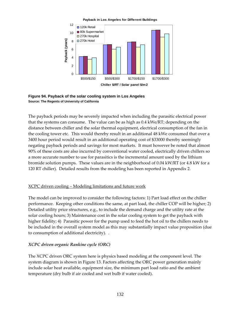
132
Figure 94. Payback of the solar cooling system in Los Angeles Source: The Regents of University of California
The payback periods may be severely impacted when including the parasitic electrical power that the systems can consume. The value can be as high as 0.4 kWe/RT; depending on the distance between chiller and the solar thermal equipment, electrical consumption of the fan in the cooling tower etc. This would thereby result in an additional 48 kWe consumed that over a 3400 hour period would result in an additional operating cost of $33000 thereby seemingly negating payback periods and savings for most markets. It must however be noted that almost 90% of these costs are also incurred by conventional water cooled, electrically driven chillers so a more accurate number to use for parasitics is the incremental amount used by the lithium bromide solution pumps. These values are in the neighborhood of 0.04 kW/RT (or 4.8 kW for a 120 RT chiller). Detailed results from the modeling has been reported in Appendix 2. XCPC driven cooling – Modeling limitations and future work The model can be improved to consider the following factors: 1) Part load effect on the chiller performance. Keeping other conditions the same, at part load, the chiller COP will be higher; 2) Detailed utility price structures, e.g., to include the demand charge and the utility rate at the solar cooling hours; 3) Maintenance cost in the solar cooling system to get the payback with higher fidelity; 4) Parasitic power for the pump used to feed the hot oil to the chillers needs to be included in the overall system model as this may substantially impact value proposition (due to consumption of additional electricity). . XCPC driven organic Rankine cycle (ORC) The XCPC driven ORC system here is physics based modeling at the component level. The system diagram is shown in Figure 13. Factors affecting the ORC power generation mainly include solar heat available, equipment size, the minimum part load ratio and the ambient temperature (dry bulb if air cooled and wet bulb if water cooled).
Payback in Los Angeles for Different Buildings
0
2
4
6
8
10
12
$500/$150 $500/$300 $1700/$150 $1700/$300
Chiller $/RT / Solar panel $/m2
Payb
ack
(yea
rs)
120k Retail80k Supermarket270k Hospital270k Hotel

133
In the design mode, the ORC inlet and outlet temperatures of the heating and cooling fluids are chosen. Based on the heat source temperature, the working fluid of the ORC and the approach to Carnot efficiency are selected based on experience. Then the solar panel area is calculated. In the off‐design mode, the modeling procedure is:
• Get the solar and weather data • With the given outlet and inlet hot fluid temperature, calculate the hot fluid flow
rate • With the available solar heat, using a loop gradually increase the heat transfer rate in
the evaporator, and then calculate the evaporating and condensing temperature. The turbine power can be calculated then. The heat transfer and the power generation are not balanced until increasing the evaporator heat transfer rate to a certain point.
• Move onto next hour • Integrate the solar power throughout the year • Economic analysis
Figure 95. Diagram of solar driven ORC Source: The Regents of University of California
Air cooled Condenser
Evaporator
Heating fluid (oil)
Cooling fluid (water)
TurbineCompressor
Phase change is assumed but constant temperature
Power out

134
XCPC driven ORC ‐ Results The design specifications of a 220kW solar driven ORC is shown in Table 21. Table 21. System specifications for solar power generation system with ORC
Source: The Regents of University of California
Here water cooled ORC with a cooling tower is assumed, which tends to have higher efficiency than an air cooled ORC. The power generation and the solar heat available throughout the year are shown in Figure 96(a) and (b). More detailed profiles for a 48‐hour period are shown in Figure 97. The peak solar heat power is likely to be higher in summer than in winter, but in general rather uniform throughout the year. The longer solar hours in summer tends to generate more power than in winter.
(a) Power generation profile (b) Solar heat available
Figure 96. Los Angeles ORC power generation and solar heat profiles Source: The Regents of University of California
Specifications Value UnitORC Design Efficiency 0.12Approach to Carnot efficiency 0.7ORC electric capacity 220 kWORC hot oil inlet temperature 150 CORC hot oil outlet temperature 120 CORC hot oil flow rate 24.1 kg/sOil design specific heat 2.5 kJ/kgCORC working fluid R245faTurbine pressure ratio 5.9Cooling fluid WaterCooling fluid flow rate 38 kg/sCooling fluid inlet temperature 15 CCooling fluid outlet temperature 25 CCooling tower pinch temperature 10 CSolar collector area 4761 m2ORC minimum part load ratio 35%
0 1000 2000 3000 4000 5000 6000 7000 8000 90000
500
1000
1500
2000
2500
3000
hours
Sol
ar h
eat a
vaila
ble
(kW
)
0 1000 2000 3000 4000 5000 6000 7000 8000 90000
50
100
150
200
250
300
Hours
Pow
er G
ener
atio
n (k
W)

135
(a) Winter profile (b) Summer
Figure 97. Typical 48-hour solar heat and electricity generation profiles in Los Angeles Source: The Regents of University of California
The annual total solar heat available and the total power generation are shown in Figure 98. The 220kW ORC delivers approximately 630 MWh of electricity per year with about 6000 MWh of solar heat. The total power generation does not vary greatly with the city. This is because it is assumed that the power generated by the ORC can always be sent to the grid, so that the power generation is only limited by the solar heat available, which does not vary with the cities in this study.
(a) Annual total solar heat available (b) Annual total power generation
Figure 98. Total solar heat and power generation in four cities Source: The Regents of University of California
The ORC operation statistics are shown in Figure 99. The ORC runs at nominal capacity for about 3200 hours per year, among which about 1000 are at full capacity or above. For ORC, when the ambient condition is favorable, e.g., very low ambient temperature, the ORC can produce slightly beyond its nominal capacity.
Jan 17-18, LA, 120k Retail
0
500
1000
1500
2000
2500
3000
0 6 12 18 24 30 36 42 48
Hour
Uni
t: kW
QsolarPower
July 23-24, LA, 120k Retail
0
500
1000
1500
2000
2500
0 6 12 18 24 30 36 42 48Hour
Uni
t: kW
QsolarPower
5894 6098 61525853
0
1000
2000
3000
4000
5000
6000
7000
Los Angeles Sacramento San Diego San Francisco
Ann
ual S
olar
Hea
t Ava
iabl
e (M
Wh)
620 638 633 627
0
100
200
300
400
500
600
700
Los Angeles Sacramento San Diego San Francisco
Ann
ual P
ower
Gen
erat
ion
(MW
h)

136
Figure 99. ORC operation statistics Source: The Regents of University of California
The overall solar heat utilization for ORC is around 0.85, higher than the typical cooling solar heat utilization ratio mentioned before, as shown in Table 22. Table 22. Detailed analysis results with solar ORC
Source: The Regents of University of California
XCPC driven ORC – Economics Similar power generation total amount directly translates to similar electricity savings, assuming the electricity cost is $0.20/kWh for all the cities. Similarly, there is no much variation with cities. The efficiency number for an XCPC driven ORC could be further lowered when factoring in pump power requirements to move the hot oil from the collectors to the ORC evaporator. This value is currently and unknown and incorporating these additional electrical demands to the system would reduce the cost savings further.
0 0.2 0.4 0.6 0.8 1 1.2 1.40
1000
2000
3000
4000
5000
6000
ORC actual power provided/Nominal capacity
Num
ber o
f hou
rs
Los Angeles Sacramento San Diego San FranciscoTotal Electricity Generated (MWh) 620 638 633 627Total Solar Hours Available 3452 3527 3545 3422Total Orc Operation Hours Provided 3186 3240 3253 3144Solar Utilization 0.85 0.85 0.84 0.85

137
Figure 100. Solar driven ORC electricity savings Figure 101, presents how payback periods could vary as a function of ORC cost/collector costs based on current estimates of electricity costs saved.
Figure 101. XCPC driven ORC payback as a function of ORC and solar collector costs Source: The Regents of University of California
The conclusion drawn from these observations is that the XCPC driven ORC is an application that requires further consideration for building applications especially in the face of rising costs of electricity.
$124,030 $127,520 $126,580 $125,350
$0
$20,000
$40,000
$60,000
$80,000
$100,000
$120,000
$140,000
Los Angeles Sacramento San Diego San Francisco
Elec
trici
ty c
ost s
aved
0
2
4
6
8
10
12
14
16
18
$1000/$150 $1000/$300 $2700/$150 $2700/$300
ORC $/kW / Solar panel $/m2
Payb
ack
(Yea
rs)
Los Angeles
Sacramento
San Diego
San Francisco

138
XCPC driven ORC – Modeling limitations and future work Currently, several major assumptions are taken in the model such as the constant temperature of the refrigerant in the evaporator and condenser. Future work to improve the model can focus on: 1) Using more detailed heat transfer models for the evaporator and the condenser; 2) Improving the turbine model to go beyond a constant efficiency assumption; 3) Using variable electricity costs to reflect the demand charges, the city‐specific rates and the time of power generation; 4) Creation of comprehensive detailed models for the collector and balance of systems which will help further refine the efficiency and cost benefits of the XCPC driven ORC systems.
Other considerations ‐ Sensitivity Analysis Sensitivity analysis has been conducted to understand the system performance characteristics. In the first study, we look at the solar cooling system payback at different cities, as shown in Figure 102. The payback in San Francisco is slightly higher, because of lower cooling load generated. With optimistic cost estimate of $500/RT for the chiller and $150/m2 for the solar panel, this creates about 7 years of payback in San Francisco and about 4 years in the other 3 cities (not factoring in parasitics). In a second study, a 50 RT chiller is used. Because a smaller system can be used more often than a larger chiller in supplying the building cooling demand, the smaller system has better payback, as shown in Figure 103. However, it should be pointed out that the chiller unit cost in $/RT tends to go higher with a smaller chiller. Therefore the benefit of using smaller chiller should be discounted.
Figure 102. Payback of solar driven cooling system at different cities Source: The Regents of University of California
Payback for 120k Retail Store
0
2
4
6
8
10
12
1416
18
$500/$150 $500/$300 $1700/$150 $1700/$300
Chiller $/RT / Solar panel $/m2
Payb
ack
(yea
rs)
Los Angeles
Sacramento
San Diego
San Francisco

139
Figure 103. Payback of solar driven cooling system with different chiller capacity
Appendix 1: Solar, weather and building raw data used in the analysis - Sample
Payback in Los Angeles for 120k Retail Store
3.7
6.1 6.6
9.1
4.3
7.27.8
10.7
0
2
4
6
8
10
12
$500/$150 $500/$300 $1700/$150 $1700/$300
Chiller $/RT / Solar panel $/m2
Payb
ack
(yea
rs)
50RT chiller120RT chiller

140
Hour Tdb Twb ITotal RH IDirect IDiffuse Cooling Total Elec Chiller ElecK K W/m2 W/m2 W/m2 kW kW kW
1 282.55 276.905 0 0.36 0 0 0 5.03E+01 02 280.95 276.368 0 0.44 0 0 0 5.03E+01 03 280.95 275.723 0 0.36 0 0 0 5.03E+01 04 279.25 274.971 0 0.43 0 0 0 5.03E+01 05 279.85 275.186 0 0.4 0 0 0 5.03E+01 06 279.25 274.864 0 0.42 0 0 0 5.03E+01 07 280.95 275.401 0 0.33 0 0 0 1.00E+02 08 282.55 276.046 37 0.27 8 29 0 2.93E+02 09 283.15 277.335 315 0.35 217 98 2.20E+01 3.31E+02 1.07E+01
10 285.35 277.872 393 0.25 193 200 7.52E+01 3.57E+02 3.68E+0111 288.15 279.161 574 0.19 340 234 1.41E+02 3.75E+02 5.40E+0112 290.35 280.342 649 0.17 372 277 1.97E+02 3.82E+02 5.88E+0113 290.35 279.913 754 0.14 553 201 1.97E+02 3.83E+02 5.89E+0114 291.45 280.557 693 0.14 522 171 2.42E+02 3.91E+02 6.31E+0115 292.05 281.094 550 0.15 400 150 2.68E+02 3.96E+02 6.57E+0116 291.45 280.557 291 0.14 193 98 2.56E+02 3.97E+02 6.45E+0117 288.75 279.698 46 0.2 17 29 1.69E+02 3.89E+02 5.64E+0118 287.05 278.624 0 0.21 0 0 1.23E+02 3.83E+02 5.26E+0119 286.45 278.194 0 0.21 0 0 1.10E+02 3.82E+02 5.16E+0120 285.95 277.872 0 0.21 0 0 9.44E+01 3.76E+02 4.62E+0121 285.35 277.442 0 0.21 0 0 0 5.03E+01 022 284.85 277.442 0 0.24 0 0 0 5.03E+01 023 283.75 277.012 0 0.27 0 0 0 5.03E+01 024 284.25 277.12 0 0.25 0 0 0 5.03E+01 025 283.75 277.012 0 0.27 0 0 0 5.03E+01 026 282.55 276.26 0 0.29 0 0 0 5.03E+01 027 283.15 276.583 0 0.27 0 0 0 5.03E+01 028 282.55 276.153 0 0.28 0 0 0 5.03E+01 029 282.55 276.153 0 0.28 0 0 0 5.03E+01 030 283.15 276.475 0 0.26 0 0 0 5.03E+01 031 280.95 275.723 0 0.36 0 0 0 1.00E+02 032 283.75 277.012 107 0.27 66 41 3.55E+01 3.37E+02 1.74E+0133 284.25 277.657 479 0.3 391 88 4.74E+01 3.43E+02 2.33E+0134 287.55 278.838 495 0.2 354 141 1.25E+02 3.73E+02 5.27E+0135 289.85 280.02 751 0.17 620 131 1.82E+02 3.80E+02 5.75E+0136 290.35 280.342 520 0.17 358 162 1.96E+02 3.82E+02 5.88E+0137 290.95 280.235 207 0.14 10 197 2.18E+02 3.86E+02 6.08E+0138 289.25 281.417 204 0.31 1 203 1.75E+02 3.84E+02 5.70E+0139 288.15 280.879 283 0.33 93 190 1.50E+02 3.83E+02 5.48E+0140 287.55 280.45 129 0.33 6 123 1.38E+02 3.82E+02 5.38E+0141 287.55 280.235 24 0.31 5 19 1.40E+02 3.83E+02 5.40E+0142 286.45 279.698 0 0.34 0 0 1.07E+02 3.81E+02 5.13E+0143 285.35 279.805 0 0.42 0 0 7.61E+01 3.66E+02 3.73E+0144 284.85 279.483 0 0.43 0 0 6.25E+01 3.59E+02 3.07E+0145 285.95 282.383 0 0.62 0 0 0 5.03E+01 046 285.95 281.631 0 0.55 0 0 0 5.03E+01 047 286.45 279.483 0 0.32 0 0 0 5.03E+01 048 286.45 279.913 0 0.36 0 0 0 5.03E+01 049 283.75 279.268 0 0.5 0 0 0 5.03E+01 050 283.75 278.624 0 0.43 0 0 0 5.03E+01 0
EnergyPlus DOE2 (LA, 120k s.f. Retail)

141
Appendix 2: Detailed modeling results for XCPC cooling using a 120 RT absorption chiller Additional information provided here includes:
• Total cooling hours needed: the hours with cooling load great than zero • Total solar heat available in MWh: total solar heat accumulation in a year with the given
solar area • Total solar heat used in MWh: total solar heat used by the chiller • Total solar heat remaining in MWh: the solar heat not used by the chiller • Electricity saved in MWh, the amount of electricity that would be used with a vapor
compression chiller with COP of 5 to replace the solar cooling • Natural gas saved in MWh, the amount of natural gas that would be used otherwise with
an absorption chiller with COP 1.3 • Solar cooling ratio, the solar cooling provided divided by the total cooling demand
Table 23 Modeling of solar driven cooling for a 80k sq ft supermarket
Note: Parasitic estimation can be done as follows LA = 3016 hours of operation with 4.8 kW for pumps (120 RT chiller estimate) implying operational costs of 14477 kWh*0.2 cents/kWh = ~$2895 per yr which is < 10% of net savings from the system. Similar estimates for other cities/building types can be done.
Los Angeles Sacramento San Diego San FranciscoTotal Cool Need (MWh) 1873 1421 2142 805Chiller Cooling Provided (MWh) 1023 905 1085 639Total Cooling Hours Needed 6171 4126 6705 3234Total Solar Hours Available 4132 4209 4208 4142Total Cooling Hours Provided 3016 2498 3210 1856Total Solar Heat Avaiable (MWh 982 1016 1025 975Total Solar Heat Used (MWh) 639 566 678 400Total Solar Heat Remaining (MW 343 451 347 576Electricity saved (MWh) 205 181 217 128Electricity cost saved $40,919 $36,199 $43,405 $25,576Natural gas saved (MWh) 769 680 816 481Natural gas cost saved $38,458 $34,022 $40,794 $24,038Collector Area (m2) 793 793 793 793Solar Cooling Ratio 0.55 0.64 0.51 0.79Solar Utilization Ratio 0.65 0.56 0.66 0.41
80k sq ft Supermarket

142
Table 24: Modeling of solar driven cooling for a 120k sq ft retail store
Table 25: Modeling of solar driven cooling for a 270k sq ft hospital
Los Angeles Sacramento San Diego San FranciscoTotal Cool Need (MWh) 2073 1910 2396 960Chiller Q Provided (MWh) 1032 959 1104 647Total Cooling Hours Need 5504 4462 5517 4827Total Solar Hours Available 3452 3527 3545 3422Total Cooling Hours Provided 3401 2976 3582 2544Total Solar Heating Avaiable (M 982 1016 1025 975Total Solar Heating Used (MWh 645 599 690 404Total Solar Heat Remaining (MW 337 417 335 571Electricity saved (MWh) 206 192 221 129Electricity cost saved $41,279 $38,351 $44,153 $25,883Natural gas saved (MWh) 776 721 830 487Natural gas cost saved $38,796 $36,045 $41,497 $24,326Collector Area (m2) 793 793 793 793Solar Cooling Ratio 0.50 0.50 0.46 0.67Solar Utilization Ratio 0.66 0.59 0.67 0.41
120k sq ft Retail Store
Los Angeles Sacramento San Diego San FranciscoTotal Cool Need (MWh) 4405 3586 4967 2308Chiller Q Provided (MWh) 1223 1158 1269 1056Total Cooling Hours Need 8695 7858 8726 8188Total Solar Hours Available 3452 3527 3545 3422Total Cooling Hours Provided 3571 3366 3659 3341Total Solar Heating Avaiable (M 982 1016 1025 975Total Solar Heating Used (MWh 765 724 793 660Total Solar Heat Remaining (MW 218 292 232 315Electricity saved (MWh) 245 232 254 211Electricity cost saved $48,930 $46,322 $50,752 $42,251Natural gas saved (MWh) 920 871 954 794Natural gas cost saved $45,986 $43,536 $47,700 $39,709Collector Area (m2) 793 793 793 793Solar Cooling Ratio 0.28 0.32 0.26 0.46Solar Utilization Ratio 0.78 0.71 0.77 0.68
270k sq ft Hospital

143
Table 26: Modeling of solar driven cooling for a 270k sq ft hotel
Los Angeles Sacramento San Diego San FranciscoTotal Cool Need (MWh) 2945 2618 3355 1583Chiller Q Provided (MWh) 1118 1023 1178 826Total Cooling Hours Need 8682 7368 8729 8139Total Solar Hours Available 3452 3527 3545 3422Total Cooling Hours Provided 3427 3063 3577 2868Total Solar Heating Avaiable (M 982 1016 1025 975Total Solar Heating Used (MWh 699 640 736 516Total Solar Heat Remaining (MW 283 377 289 459Electricity saved (MWh) 224 205 236 165Electricity cost saved $44,737 $40,937 $47,134 $33,047Natural gas saved (MWh) 841 770 886 621Natural gas cost saved $42,046 $38,475 $44,299 $31,059Collector Area (m2) 793 793 793 793Solar Cooling Ratio 0.38 0.39 0.35 0.52Solar Utilization Ratio 0.71 0.63 0.72 0.53
270k sq ft Hotel

144
2.9. Task 10 Three competing XCPC design concepts were formulated in Task 4.
1. All glass dewar: Direct Flow
2. All glass dewar filled with thermal fluid: Indirect Flow
3. Metal absorber with glass‐to‐metal seal
In Task 7, relying on only off‐the‐shelf components, the thermal efficiency of each design was estimated as a function of operating temperature. It was found that the “Direct Flow” design and the “Metal Absorber with Glass‐to‐Metal Seal” design could nearly achieve the performance goal of 50% thermal efficiency at 400ºF. This was a very positive result. But before selecting a “Preferred XCPC Design” (Task 11 of this project), the extent that future component could improve the performance of the top two XCPC design alternatives development (Phase 2 activities during the second year of this project) was quantified. The “Fluid‐filled dewar” design was not considered since Task 7 showed that the concept offers little potential to achieve the performance goal.
Component Improvements There are a number of ways to increase the performance of the XCPC through the development of improved components that can then be incorporated into the design of an advanced XCPC. Some of these component improvements require a significant R&D effort, while others do not and can be implemented quite quickly into an improved XCPC design. Four primary component improvements were identified. The difficulty of successfully implementing various component improvements was examined, and their performance impacts were quantified.
A. Improved Selective Coating
B. Anti‐Reflective Coating on Glass
C. Higher Reflectance CPC
D. Thicker Absorber (applies only to Metal absorber with glass‐to‐metal seal) A) Improved Selective Coating First, the “Metal absorber with glass‐to‐metal seal” design, which uses a thin metallic foil that has a black selective coating, was considered.
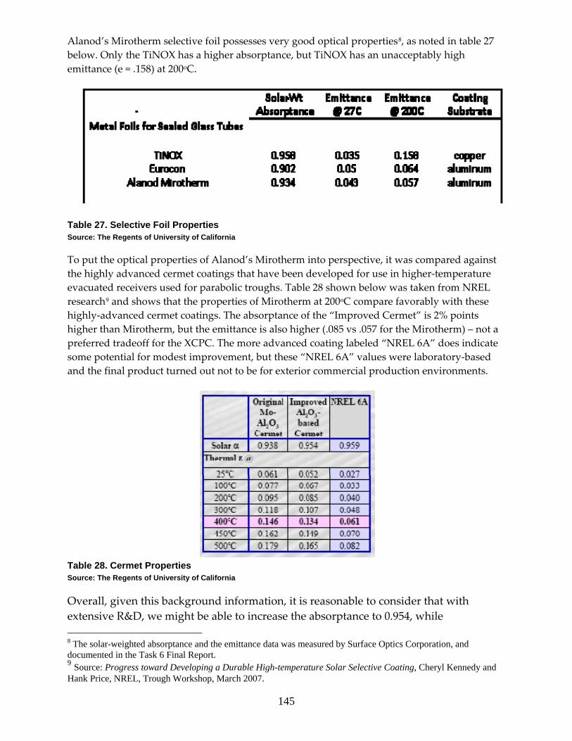
145
Alanod’s Mirotherm selective foil possesses very good optical properties8, as noted in table 27 below. Only the TiNOX has a higher absorptance, but TiNOX has an unacceptably high emittance (e = .158) at 200oC.
Table 27. Selective Foil Properties Source: The Regents of University of California
To put the optical properties of Alanod’s Mirotherm into perspective, it was compared against the highly advanced cermet coatings that have been developed for use in higher‐temperature evacuated receivers used for parabolic troughs. Table 28 shown below was taken from NREL research9 and shows that the properties of Mirotherm at 200oC compare favorably with these highly‐advanced cermet coatings. The absorptance of the “Improved Cermet” is 2% points higher than Mirotherm, but the emittance is also higher (.085 vs .057 for the Mirotherm) – not a preferred tradeoff for the XCPC. The more advanced coating labeled “NREL 6A” does indicate some potential for modest improvement, but these “NREL 6A” values were laboratory‐based and the final product turned out not to be for exterior commercial production environments.
Table 28. Cermet Properties Source: The Regents of University of California
Overall, given this background information, it is reasonable to consider that with extensive R&D, we might be able to increase the absorptance to 0.954, while 8 The solar-weighted absorptance and the emittance data was measured by Surface Optics Corporation, and documented in the Task 6 Final Report. 9 Source: Progress toward Developing a Durable High-temperature Solar Selective Coating, Cheryl Kennedy and Hank Price, NREL, Trough Workshop, March 2007.

146
maintaining the 200oC emittance at 0.05. Figure 104 below is a comparison of the impact this improved selective coating should have on the XCPC’s thermal efficiency. Note that at our 200oC design point, it was calculated that the thermal efficiency would increase from 46.4% to 50.5%. Figure 104. Horizontal Glass to Metal Tube Efficiency Source: The Regents of University of California
It was also useful to compare this advanced cermet coatings with the coatings used within the all‐glass dewars, which are tabulated in Table 29 below. Solar‐Wt Emittance Emittance Coating Chinese all‐glass dewars Absorptance @ 27C @ 200C Substrate
Paradigma 0.883 0.1 0.15 glass Tsinghua 0.923 0.05 0.074 glass SunRain 0.913 0.047 0.088 glass
Table 29: All Glass Dewar Advanced Cermet Coatings
The Tsinghua dewar has the best optical properties of the dewar coatings. The absorptance of the Tsinghua coating is about 1% point lower than for Mirotherm, and the emittance at 200°C is slightly higher (0.074 vs. 0.064 for the Mirotherm). Achieving the improved selective coating properties we noted above (absorptance = .954 and emittance = .05 at 200°C), was expected to be more difficult for the all‐glass dewars. This is because the emittance of glass is high, while the emittance of aluminum (or copper and most other metals) is relatively low. To achieve low

147
emittance on glass requires that a highly reflective layer be deposited onto the glass, an extra requirement compared to metal‐based selective foils. In any case, for the sake of continuity and ease of comparison, we have made these same assumptions for the improved coating (i.e. an absorptance of 0.954 and an emittance of 0.05).
Figure 105. Horizontal Dewar Efficiency Source: The Regents of University of California
As shown in Figure 105 above for these assumptions (absorptance = .954 and emittance = .05 at 200°C), the “Direct Flow” collector efficiency increases to 55% with the improved selective coating, compared to a baseline collector efficiency at 200°C of 50%, B) Anti‐Reflective Coating on Glass The solar‐weighted transmittance of the borosilicate glass used in the dewars was found to be 91.7%, as reported in the Task 6 Final Report. With the addition of an anti‐reflective layer to both surfaces of the glass cylinder (just the 57 mm OD glass cylinder, in the case of the all‐glass dewars), the solar‐weighted transmittance can be increased to 96%, see Figure 106. The most cost‐effective method to add the anti‐reflective coating is with the application of a sol‐gel coating – typically implemented as a dip process, followed by a bakeout process. Several solar companies have successfully developed this process for parabolic trough evacuated receivers in the last ten years, including Abengoa/Solucar and Schott Solar (for their highly advanced evacuated receivers). But none of the millions of the evacuated tubes that are manufactured in China employed this AR‐coating technology.

148
Figure 106. Transmittance with Anti Reflective Coating Source: The Regents of University of California
The transmittance of borosilicate glass vs wavelength is shown in the figure 107 below, both with the addition of a sol‐gel anti‐reflective coating and without. Figure107. Transmittance by Wavelength Source: The Regents of University of California
With the addition of the anti‐reflective coatings to the glass, the collector efficiency at 200oC of the baseline “Metal absorber with glass‐to‐metal seal” collector increases from 46.4% to 49.5%. Figure 108.

149
Figure 108. Metal Absorber Collector with AR Source: The Regents of University of California
Similarly, with the addition of anti‐reflective coatings to the glass dewars for the “Direct Flow” design, the collector efficiency increases from 50% at 200oC to 53%. Figure 109. Figure 109. Direct Flow Dewar with AR Source: The Regents of University of California
C Higher Reflectance CPC For our baseline XCPC designs, we assumed the use of Alanod Miro Sun, an advanced aluminum reflector with a specialized coating that increases the reflectance as well as increasing outdoor weatherability. The solar‐weighted hemispherical reflectance of Alanod Miro Sun is

150
91.9%, but it measures 86% with the Devices and Services portable specular reflectometer Model 15R (D&S), which measures at 660 nm, a wavelength that happens to be a bit low with Miro Sun and thereby would be expected to provide a reading on the low side. The D&S also excludes light that is scattered, since it is intended to just measure specularly‐reflected light. Given the high acceptance angles of the CPCs, we expected that performance would be more closely governed by hemispherical reflectance than specular reflectance, but would be somewhere in between. To be conservative, in our modeling efforts we assumed a reflectance value of 90%. Metallized polymer films are another class of reflective surfaces. A relatively recent silvered film has been developed by NREL and ReflecTech (www.reflectechsolar.com) that has recently reached commercial status after years of R&D. The hemispherical reflectance and the specular reflectance (using the D&S) of ReflecTech film both exceed 94%. The measured hemispherical reflectance vs. wavelength values are shown in Figure 110 for Alanod’s Miro Sun and the ReflecTech film. These measurements were obtained at NREL.
Figure 110. Spectral Reflectance Source: The Regents of University of California
Alanod (www.alanod.de) was also expected to offer a higher‐reflectance alternate to their Miro Sun. This new reflector utilizes silver in order to achieve a higher reflectance than the aluminum based Miro Sun. Alanod introduced this new material for commercial use in 2008. The materials turned out to be only for protected (lighting and TV displays) environments. With the use of ReflecTech film, the collector efficiency at 200oC of the baseline “Metal absorber with glass‐to‐metal seal” collector increases from 46.4% to 48.3%.

151
Figure 111. Metal Absorber with Reflectec Source: The Regents of University of California
Similarly, with the use of ReflecTech film for the “Direct Flow” design, the 200oC collector efficiency increases from 50% to 52 %.
Figure 112. Direct Flow with Reflectec Source: The Regents of University of California

152
Thicker Absorber (applies only to “Metal absorber with glass-to-metal seal” design) The design pictured in Figure 113 to the right uses an evacuated glass tube with a glass-to-metal seal at one end that maintains the vacuum to insulate the metal absorber. The metal absorber is a thin cylindrical metallic fin with a selective coating that enables high solar absorptance and reduces radiative heat loss. The fin is welded to a metal counter flow tube. The heat absorbed by the fin is transferred to the manifold by the circulating fluid within the metal tube.
Figure 113. Metal Absorber Design Source: The Regents of University of California
Our analysis of this design has shown that the thermal performance is significantly affected by the thickness of the cylindrically‐shaped metallic absorber, because the cylindrical absorber acts as a fin since it must conduct heat around its entire surface to the point of contact with the copper tube where all the heat is extracted. Figure 114 shows how the XCPC collector efficiency is affected by the thickness of the absorber. It indicates that an absorber thickness of at least 0.6 mm is needed to achieve good results with an aluminum absorber. Our baseline design (using Alanod’s Miro Sun absorber) uses an aluminum absorber of 0.8 mm. It is clear from the figure that there is virtually no performance incentive to increase the absorber thickness above this baseline 0.8 mm thickness.

153
Figure 114. Metal Absorber Thickness
C) AR Coating Combined with Higher Reflectance CPC In this section, we evaluate the addition of two simultaneous improvements – the two improvements that can be most assuredly incorporated with the little technical risk and at little or no cost (past any R&D and testing activities). The two improvements that are most readily incorporated into an advanced XCPC are the AR‐coating and the higher reflectance CPC. The higher reflectance CPC can be most easily accomplished with the use of ReflecTech silvered film. And as noted previously, Alanod is working on a higher reflectance material. The AR‐coating will require a significant R&D effort, but not one that has any risk of failure because the addition of sol‐gel coatings on borosilicate glass is well understood. Figure 115 below shows that the collector efficiency of the “Metal absorber with glass‐to‐metal seal” design at 200oC is estimated to increase from the baseline of 46.4% up to 52.6% with the addition of both the AR‐coating and the higher reflectance CPC.

154
Figure 115 Metal Absorber with AR and Reflectec Source: The Regents of University of California
Figure 116 shows that the 200oC collector efficiency of the “Direct Flow Dewar” design is estimated to increase from the baseline of 50% up to 56% with the addition of both the AR-coating and the higher reflectance CPC.

155
Figure 116. Direct Flow Tube with AR and Reflectec Source: The Regents of University of California
Summary Table Table 30 summarizes the findings of this Task 10 analysis.
Table 30. Component Improvement Summary Source: The Regents of University of California
2.10. Task 11 Summary This Task identified a single preferred external compound parabolic concentrator (XCPC) design based on:
performance estimates of Task 7, cost estimates of Task 8, and Task 10 analysis of the potential for improvements to each major XCPC design option.
Difficulty (1=easy , 5=difficult) Thermal Efficiency at 200 deg CComponent Improvement Direct Flow Glass-to-Metal Seal Direct Flow Glass-to-Metal Seal
Improved Selective Coating 4 5 55% 50.5%A-R Coated Glass 2 2 53% 48.3%
Higher Reflectance CPC 1 1 52% 48.3%Thicker Absorber (1 mm) N/A 2 N/A 47.0%
Higher Reflectance + A-R Coated Glass N/A 2 56% 52.6%Baseline = 50% Baseline = 46.4%

156
The task provides the XCPC design down‐select methodology and all significant data behind the methodology. The methodology is based on a matrix‐based evaluation of solar collector system and component characteristics (e.g. cost and efficiency) that are important in determining the technology’s overall desirability for likely application(s). The characteristics used for collector selection are:
• Performance o Efficiency o Actual annual energy production
• Risk o Technical o Marketing – reputation/potential for leakage
• Cost • O&M – cost and convenience • Manufacturability • Installation • Robustness, durability/lifetime
The purpose of this down‐select process is to determine the single preferred XCPC design that is to be the focus of further work under this project effort. It should be noted that much of the technical data, as well as some of the more qualitative information used in this down‐select process, is based on theoretical information and models that have not yet been validated with field testing. Therefore, although this report recommends a preferred XCPC design for further consideration, this recommendation will be confirmed upon field testing the recommended design – for general operability and performance model validation – as part of Task 15 and Task 16. Collector Design Concepts The XCPC collector cost and performance goals set forth in this agreement were as follow:
• 50% collector efficiency at 204oC (400 oF) • Production cost (high volume) less than $108/m2 ($10/ft2).
Originally (Task 4), the Contract design team (SolFocus and UC Merced) formulated three competing, conceptual‐level designs for the XCPC collector. All three designs were believed to have the potential to reach the Contract performance and cost goals. The three original design concepts were as follow:
1. All glass dewar: direct flow Figure 117 2. All glass dewar filled with heat transfer fluid: indirect flow
with metal pipe with heat pipe
3. Metal absorber with glass‐to‐metal seal Figure 118 with metal tube with heat pipe
All features of the above design concepts are described in detail in the Contract Task 4 report.

157
Results from performance analysis documented in the Draft Preliminary Design Report under Task 7 clearly illustrated that the indirect flow collector concept (design concept #2, above) likely did not have the potential to meet our performance goals of 50% efficiency at 200oC. Therefore, this design concept was removed from consideration in our down‐select process. Further preliminary analysis showed that for the two remaining design concepts, collector orientation was potentially an influential factor. Therefore, the following design concepts and variations were considered for the final Task 7 performance analysis and Task 8 cost analysis:
1. All glass dewar: direct flow a. east‐west orientation b. north‐south orientation
2. Metal absorber flow‐through a. east‐west orientation b. north‐south orientation
3. Metal absorber heat pipe (only north‐south orientation possible)
Figure 117. All glass dewar: direct flow Figure 118. Metal absorber with glass-to-metal seal Source: The Regents of University of California Source: The Regents of University of California
Collector Performance Analysis The project team has looked to the collectors’ projected performance as a significant determinant in the down‐select process. A precursory performance analysis of the five original design concepts was first performed as part of Task 4. The Task 6 Component Characterization Report provided the performance‐critical, material properties of the off‐the‐shelf components that are being considered for the XCPC. The projected collector efficiency as a function of heat‐transfer‐fluid temperature was calculated as part of Task 7. And the Task 10 Report assessed ways in which the collector efficiencies might be improved through R&D, and quantified the impact this improvements would make on the XCPC collector designs. The heat pipe design was eliminated from the performance analysis of the down‐select process because the heat pipe analysis performed by United Technologies Research Center, which is included in Task 6, determined that it did not have temperature capability above 160oC.
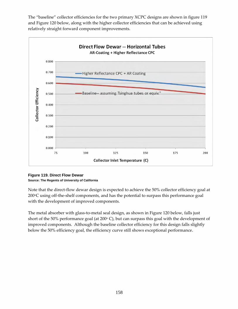
158
The “baseline” collector efficiencies for the two primary XCPC designs are shown in figure 119 and Figure 120 below, along with the higher collector efficiencies that can be achieved using relatively straight forward component improvements.
Figure 119. Direct Flow Dewar Source: The Regents of University of California
Note that the direct‐flow dewar design is expected to achieve the 50% collector efficiency goal at 200oC using off‐the‐shelf components, and has the potential to surpass this performance goal with the development of improved components. The metal absorber with glass‐to‐metal seal design, as shown in Figure 120 below, falls just short of the 50% performance goal (at 200o C), but can surpass this goal with the development of improved components. Although the baseline collector efficiency for this design falls slightly below the 50% efficiency goal, the efficiency curve still shows exceptional performance.

159
Figure 120. Metal Absorber Source: The Regents of University of California
In Task 5, the annual performance modeling tool f‐Chart was determined to be an appropriate analysis tool for this stage of the XCPC collector development. F‐chart (see www.fchart.com) uses the following as input parameters: optical efficiencies, acceptance half angle, incident angle modifiers (as determined by the project’s raytrace model) and heat‐loss coefficients (as determined by the project team’s heat transfer analysis). F‐Chart was used for the analysis presented in this report to examine and compare the area‐normalized, annual performance of the two design concepts and orientations. The results of this analysis for two California climates – San Francisco (diffuse solar resource) and Daggett (strong direct‐normal solar resource) – are shown in Figure 121 and Figure 122 respectively.

160
Figure 121. Annular Performance in a Diffused Environment Source: The Regents of University of California
Figure 122. Annular Performance in a Direct Solar Environment Source: The Regents of University of California
In agreement with the efficiency curves, the f‐Chart results predict slightly better performance on the part of the all‐glass, direct‐flow dewar. Not predicted by the efficiency calculations, the f‐Chart results predict an added performance benefit from the north‐south orientation in locations with non‐negligible diffuse solar radiation, such as in San Francisco. The enhanced
XCPC Solar Thermal Energy Production vs. MonthSan Francisco, CA
0
0.05
0.1
0.15
0.2
0.25
1 2 3 4 5 6 7 8 9 10 11 12
Month
Prod
uctio
n pe
r Are
a, G
J/m
2
Dewar; East-WestDewar; North-SouthGlass-to-Metal; East-WestGlass-to-Metal; North-South
XCPC Solar Thermal Energy Production vs. MonthDaggett, CA
0
0.05
0.1
0.15
0.2
0.25
0.3
1 2 3 4 5 6 7 8 9 10 11 12
Month
Prod
uctio
n pe
r Ar
ea, G
J/m
2
Dewar; East-WestDewar; North-SouthGlass-to-Metal; East-WestGlass-to-Metal; North-South

161
benefit of the north‐south orientation in non‐desert climate zones is believed to be a result of the acceptance angle. The acceptance half angle for the north‐south reflector design is 60o and for the east‐west reflector design, it is 35o. Under diffuse weather conditions (e.g. overcast, cloudy or humid) a more significant fraction of the solar resource is scattered and, therefore, a wider acceptance angle becomes more of a factor to enhancing the collector’s performance. Collector Cost Analysis The Task 8 Draft XCPC Cost Comparison Report provides a bill of materials (BOM) analysis for each of the final design concepts and variations listed above. The results of this analysis are in Table 31.
Table 31. Cost Comparison of XCPX Design Concepts in High Volume Production (10,000 tubes) Source: The Regents of University of California
The BOM cost analysis results favor the direct‐flow all‐glass dewar designs. The all‐glass dewar collectors are estimated to be from 24% to 32% lower in cost than the metal absorber with glass‐to‐metal seal collectors. But it is notable that the metal absorber with glass‐to‐metal seal
XCPC concept All-glass dewar: Direct Flow
All-glass dewar: Direct Flow
Metal absorber flow-through
Metal absorber flow-through
Metal absorber heat pipe
Orientation East-West North-South East-West North-South North-South
Bill of Materials
Absorber tubeTube type Sunrain All-glass
dewar with improved selective coating (TTY-MC)
Sunrain All-glass dewar with improved selective coating (TTY-MC)
Beijing Eurocon metal absorber tube with counterflow insert
Beijing Eurocon metal absorber tube with counterflow insert
Beijing Eurocon metal absorber tube with heat pipe
Length of tube 1800 mm 1800 mm 1800 mm 1800 mm 1800 mmOD of tube 58 mm 58 mm 65 mm 65 mm 65 mmDiameter of absorber 47 mm 47 mm 56 mm 56 mm 56 mmPrice of one tube $3.20 $3.20 $22.00 $22.00 $21.00Price of tubes [per aperture of reflector (m2)] $6.40 $9.94 $37.19 $58.27 $55.62
ReflectorMaterial Alanod Alanod Alanod Alanod AlanodReflectivity 90% 90% 90% 90% 90%Acceptance angle ± 34º ± 60º ± 34º ± 60º ± 60ºTrunction 20% 20% 20% 20% 20%Length of reflector (mm) 1860 1860 1860 1860 1860Width (mm) of reflector opening (incl 1mm spacing) 269 173 318 203 203Depth (mm) of reflector 212 83 261 97 97Arclength of reflector (mm) 562.6 278.8 685.6 327.8 327.8Aperture of one reflector (m2) 0.50034 0.32178 0.59148 0.37758 0.37758Reflector material needed per tube (m2) 1.046436 0.518568 1.275216 0.609708 0.609708Price of reflector material (incl. support structure) per m2 $15.00 $15.00 $15.00 $15.00 $15.00Price of reflector per tube $15.70 $7.78 $19.13 $9.15 $9.15Price of reflector [per aperture of reflector (m2)] $31.37 $24.17 $32.34 $24.22 $24.22
ManifoldLength of manifold ~2.2m ~2.2m ~2m ~2.1m ~2.1mTubes per manifold 8 12 6 10 10
Price of manifold (Eurocon) $180.00 $190.00 $96.00 $106.00 $80.00Estimated price of manifold in mass production $90.00 $95.00 $48.00 $53.00 $40.00Price of manifold per tube $11.25 $7.92 $8.00 $5.30 $4.00Price of manifold [per aperture of reflector (m2)] $22.48 $24.60 $13.53 $14.04 $10.59
Collector frame and rackDimensions of one collector ~2.2m x 2m ~2.2m x 2m ~2m x 2m ~2.1m x 2m ~2.1m x 2mPrice of one frame including rack (Eurocon) $176.00 $176.00 $176.00 $176.00 $176.00 Estimated price of one frame including rack in mass production $88.00 $88.00 $88.00 $88.00 $88.00 Price of one frame including rack per tube $11.00 $7.33 $14.67 $8.80 $8.80Price of frame and rack [per aperture of reflector (m2)] $21.99 $22.79 $24.80 $23.31 $23.31
Total BOM [per aperture of reflector (m2)] $82.24 $81.51 $107.86 $119.83 $113.74Total BOM [per aperture of reflector (sf)] $7.64 $7.58 $10.02 $11.14 $10.57

162
collector is estimated to cost $107.86/m2 ($10.02/ft2), which is right at our cost goal target, and the north‐south version is within 11% of the cost target. Further, although the BOM cost estimates point to the dewar designs, this cost calculation is only one component of the complete cost analysis that should be performed for the final, single collector down select. The Contractor recommends that, as part of the final selection, we perform analysis to determine the levelized cost of energy (LCOE, $/kWh) and the installed cost per generation capacity ($/kW) for each design concept and orientation variation. Collector Down Select Table 32 provides the down‐select matrix for the XCPC collectors under consideration. Collector All Glass
Dewar – Direct Flow
All Glass Dewar – Direct Flow
Metal Abs. with Glass-to-Metal Seal and Counter Flow-Through
Metal Abs. with Glass-to-Metal Seal and Counter Flow-Through
Metal Abs. with Glass-to-Metal Seal and Heat Pipe
Orientation East-West North-South East-West North-South
North-South
Cost, $/m2 82.24
81.51 107.86 119.83 113.74
Annual Energy Production, GJ/m2 (Daggett, CA)
2.617
2.798
2.086
2.066
Unknown
Cost, $/GJ (Dagett, CA) 31.43 29.13 51.70 58.00 Unknown Annual Energy Production, GJ/m2 (San Francisco, CA)
1.659
1.868
1.228
1.265
Unknown
Cost, $/GJ (San Francisco, CA)
49.57 43.63 87.83 94.73 Unknown
Collector Efficiency (@200oC, current properties)
50%
46%
47%
40%
Unknown
Collector Efficiency (@200oC, improved properties)
57%
52%
53%
46%
Unknown
Performance Profile (i.e. hourly load matching)
Unknown Unknown Unknown Unknown Unknown
O&M (cost and convenience)
Good
Good
Good
Good
Good
Manufacturability Requires modest development
Requires modest development
Excellent
Excellent
Requires significant development
Robustness, Durability, Lifetime
Requires modest development
Requires modest development
Excellent
Excellent
Requires significant development

163
Risk: Technical/ Marketability
Moderate Moderate Low Low High
Low-Moderate
Low-Moderate
Low-Moderate
Low-Moderate
High
Potential for Improvement
Excellent Excellent Low-Good Low-Good Unknown
Table 32. Down-Select Matrix Source: The Regents of University of California
Conclusions The down‐select matrix in Table 32 shows that the first case under consideration – the direct‐flow all‐glass dewar – has the best predicted performance of all the collector designs under consideration. At 200oC, the project team’s heat transfer analysis, optical analysis, and the measured material properties show this collector’s efficiency projection leads the other projections by a range from 6% to 25%. Although this collector shows better performance capability and lower cost, the metal absorber with glass‐to‐metal seal design is closer to commercial readiness as well as showing an impressive projected performance. Readiness for commercialization is also a significant consideration for the collector of choice for this project. The glass‐to‐metal seal collector design currently has better manufacturability, and better durability/robustness and lower technical risk (i.e. lower risk in the event of glass tube breakage) than the all‐glass dewar design. Because the all‐glass dewar design uses the glass tube directly for containing the heat transfer fluid, it has a higher risk for:
• potential heat transfer fluid leaks between the glass dewar and the manifold, • tube breakage resulting in a significant heat transfer fluid spill.
Although the required technical development effort necessary to overcome these risks is not viewed as significant, it is somewhat uncertain. Therefore, the design selected as the preferred design for consideration under this project is the metal absorber with glass‐to‐metal seal. This collector design is very close to commercialization in addition to showing excellent performance prospects. The project team’s heat transfer analysis shows the east‐west orientation design has fairly significant efficiency benefits (47% vs. 40% at 200oC) but our f‐Chart analysis results show that, because of the north‐south concentrator’s wider acceptance angle, there may be benefits to the north‐south orientation design. To determine which orientation results in the best performance, the project team recommends testing both orientation designs in multiple climates and more detailed modeling.
2.11. Task 12 This report describes the detailed design of the XCPC that was selected in Task 11. The selected design is called “Metal absorber with glass‐to‐metal seal and counter flow tube.” This design uses an evacuated glass tube with a glass‐to‐metal seal at one end that maintains the vacuum to insulate the metal absorber (Figure 123 and 124). The metal absorber is a thin cylindrical metallic fin with a selective coating that enables high solar absorptance and reduces radiative heat loss. The fin is welded to a metal counter flow tube. The heat absorbed by the fin is transferred to the manifold by the circulating fluid within the metal tube.

164
Figure 123. Schematic of XCPC Design Source: The Regents of University of California
Figure 124. Cross section of absorber tube Source: The Regents of University of California
The XCPC design consists of the following elements:
• Evacuated glass tube with metal absorber • Manifold • Reflector
1 Inlet cold fluid2 Pump3 Outlet hot fluid4 Manifold5 Glass-to-metal seal6 Evacuated glass tube7 Copper fin with
selective coating8 Counter flow metal tube9 External reflector
12
34
5
7
6
89
67 8
9
1 Inlet cold fluid2 Pump3 Outlet hot fluid4 Manifold5 Glass-to-metal seal6 Evacuated glass tube7 Copper fin with
selective coating8 Counter flow metal tube9 External reflector
12
34
5
7
6
89
67 8
9

165
• Frame Evacuated Glass Tube The evacuated glass tube (including the metal absorber) is made by Beijing Eurocon Solar Energy Tech. Company in Beijing, China. The tube has the following dimensions:
Diameter of outer tube wall: 65 mm Diameter of inner tube wall: 61.8 mm Length: 1,800 mm
The metal absorber is a cylindrical aluminum fin of 1mm thickness, 56 mm in diameter and 1,720 mm long. It is coated with a selective coating that was developed by Beijing Eurocon Solar Energy Tech. Company. The copper counter‐flow tube conducts the heat transfer fluid from the manifold through the absorber tube back to the manifold. The counter‐flow tube consists of an inner tube (I.D. 6 mm, O.D. 7 mm) and an outer tube (I.D. 10.5 mm, O.D. 12 mm). The counter‐flow tube is welded onto the metal absorber. The glass tube (including the metal absorber and counter‐flow tube) is depicted in Figure 125. The transmittance of the glass tube was measured at NREL. The solar‐weighted transmittance was found to be 91.7%, which is a good result. We also measured the absorptance and emittance of the absorber. The absorptance was found to be 0.904, with an emittance of 0.050 at room temperature, and an emittance of 0.064 at 200oC. Manifold The copper manifold is made by Beijing Eurocon Solar Energy Tech. Company in Beijing, China. The manifold collects the fluid that is circulated through the parallel absorber tubes. A drawing of the manifold is depicted in Figure 126. Reflector The reflector material is a polished aluminum reflector made by Alanod, Germany. We use the Alanod MiroSun product. Its solar‐weighted hemispherical reflectance is 91.9%. The concentration ratio of the reflector is 1.15 (if the tubes are oriented in North‐South direction) and 1.8 (in East‐West orientation). The acceptance angle is ±60º (North‐South) and ±34º (East‐West). The truncation is 20% in both orientations. The shape of the reflector for both directions is depicted in Figure 127. Frame The wooden frame is made by Great Spaces Inc. in Merced, California. It holds six absorber tubes, the reflector and the manifold. The frame contains seven wooden ribs for each tube that are mounted on a wooden ground plate. The ribs provide support for the reflector foil. The Alanod reflector foil is glued onto the wooden ribs. The ribs are cut to the shape that is necessary to achieve the optical concentration. The absorber tubes are then placed

166
perpendicular to the ribs. A drawing of the frame (for the North‐South orientation) is depicted in Figure 128.
Figure 125. Evacuated glass tube with metal absorber (all units in mm) Source: The Regents of University of California
List of possible vendors of the parts for the XCPC prototype: Evacuated glass tube (including the metal absorber) and manifold Beijing Eurocon Solar Energy Tech. Co. Ltd. No. 30 Xueyuan Road Haidian District Beijing 10083 China Reflector Alanod P.O. Box 3910 180 Leadville Ave. N Ketchum, Idaho 83340 Frame Great Spaces USA 360 Grogan Ave Merced, CA 95340

167
Figure 126. Manifold for North-South orientation [all units in mm] Source: The Regents of University of California
Figure 126b: Manifold for East-West orientation [all units in mm] Source: The Regents of University of California
-60
-40
-20
0
20
40
60
-150 -100 -50 0 50 100 150
(mm)
(mm
)

168
Figure 127a. Cross section of reflector for North-South orientation Source: The Regents of University of California
Figure 127b. Cross section of reflector for East-West orientation Source: The Regents of University of California
-100
-50
0
50
100
150
200
-150 -100 -50 0 50 100 150
(mm)
(mm
)

169
Figure 128. End view (upper drawing) and length view (three lower drawings) of frame for XCPC system in North-South orientation Source: The Regents of University of California
2.12. Task 13 This report confirms that two prototype versions of the XCPC have been manufactured according to the drawings as described in the Task 12 report. One version includes the absorber tubes in North‐South orientation, the other version in East‐West orientation. The picture below shows the North‐South version.

170
2.13. Task 14 Expected optical efficiency and Incident Angular Modifier (IAM) The expected optical efficiency for the XCPC in East‐West orientation is 63.9% in normal incidence, and 67.5% averaged over all incidence angles between 0 degree and 34 degrees. The expected IAM curve is depicted in Figure 129.
Figure 129. Expected Optical Efficiency and Incidence Angle Modifier for East-West orientation Source: The Regents of University of California
Expected thermal efficiency The expected thermal efficiency of the XCPC is depicted as the blue lines in Figure 130. The solid blue line (“Eurocon horizontal”) describes the expected thermal efficiency of the XCPC in East‐West orientation, the dashed blue line (“Eurocon vertical”) in North‐South orientation.
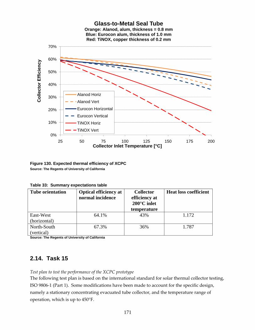
171
Figure 130. Expected thermal efficiency of XCPC Source: The Regents of University of California
Table 33: Summary expectations table Tube orientation Optical efficiency at
normal incidence Collector
efficiency at 200°C inlet
temperature
Heat loss coefficient
East-West (horizontal)
64.1% 43% 1.172
North-South (vertical)
67.3% 36% 1.787
Source: The Regents of University of California
2.14. Task 15 Test plan to test the performance of the XCPC prototype The following test plan is based on the international standard for solar thermal collector testing, ISO 9806‐1 (Part 1). Some modifications have been made to account for the specific design, namely a stationary concentrating evacuated tube collector, and the temperature range of operation, which is up to 450°F.
0%
10%
20%
30%
40%
50%
60%
70%
25 50 75 100 125 150 175 200
Col
lect
or E
ffici
ency
Collector Inlet Temperature [°C]
Glass-to-Metal Seal TubeOrange: Alanod, alum, thickness = 0.8 mmBlue: Eurocon alum, thickness of 1.0 mmRed: TiNOX, copper thickness of 0.2 mm
Alanod Horiz
Alanod Vert
Eurocon Horizontal
Eurocon Vertical
TiNOX Horiz
TiNOX Vert

172
The tests to be performed in Task 16 will include:
• Collector time constant • Collector thermal efficiency • Collector optical efficiency • Collector incident angle modifier • Pressure drop across the collector
Description of Test Loop The test facility uses is a closed loop system that includes a circulating oil temperature controller with integrated pump and expansion tank (see Figure 131). The circulating oil temperature controller provides a selectable constant temperature (up to 500°F) to the heat transfer fluid that is circulated through the collector. The loop further includes a flow meter, temperature sensors before and after the collector, and a calorimeter. The calorimeter is described in detail below. The solar collector is mounted on a dual axis tracker to allow the measurement of collector performance under controlled incidence angles. The test facility further includes a meteorological station with a Precision Spectral Pyranometer that is mounted on the same tracker as the solar collector, a Normal Incidence Pyrheliometer mounted on a separate dual‐axis tracker, a thermometer to measure the ambient temperature, and an anemometer.

173
Figure 131. Schematic of Test Facility Source: The Regents of University of California
~1 gpm
Distance ~15 foot
1 ½” NPT Oil Inlet
30 gpm
1 ½” NPT Oil Outlet
½ “ NPT Cooling Water Inlet
½ “ NPT Cooling Water Outlet
Chromalox CMXO Circulating Oil Temperature Control System
Sun Tracker (Moving Structure)
Flexible pipe
Flexible pipe 6 kW Heater
Pump 30 gpm
Expansion Tank
Cooling module
1a
1b
2
3
4 5 6a
Solar collector(s)
6b 2 kW Calorimeter 6
d
1c
6c
tube

174
The data from the flow meter, the temperature sensors and the meteorological station are recorded through a data acquisition system. Instrumentation Circulating oil temperature controller: Chromalox CMXO 6kW (with integrated pump and expansion tank) Temperature sensors: Type‐K thermocouples from Omega Flow meter: Micro Motion Coriolis F‐Series sensor Flow control valve: Valtek ½” Flow Top Control Valve Back pressure regulating valve: Jordan: 1” 50‐100‐S6‐I5‐S6‐Y‐8‐21‐S6‐MD Pressure Control Valve Sun tracker: Wattsun AZ‐125 dual axis tracker Calorimeter: Custom made by Valin Inc. Pyranometer: Eppley Precision Spectral Pyranometer Pyrheliometer: Eppley Normal Incidence Pyrheliometer Amplifiers: Agilent 34970A Data Acquisition/Switch Unit Data logger: Obvius A8811 and A8923 Test Procedure for Collector Time Constant Testing will be performed outdoors with a solar irradiance on the plane of the collector aperture greater than 800 W/m2. The heat transfer fluid will be circulated through the collector at the same flow rate as used during collector thermal efficiency testing. Initially the collector’s aperture will be shielded from solar radiation by means of a solar‐reflecting cover, and the temperature of the heat transfer fluid at the collector inlet will be approximately equal to the ambient air temperature. When a steady state has been reached, the cover will be removed and measurements of the collector fluid inlet temperature (tin), the collector fluid outlet temperature (te), and the surrounding air temperature (ta) will be taken until steady‐state conditions have been reached again. A steady state condition is assumed to exist when the outlet temperature of the fluid varies by less than 0.05°C per minute. The difference between the temperature of the fluid at the collector outlet and that of the surrounding air will be measured against time, beginning with the initial steady‐state condition and continuing until the second steady state has been achieved at a higher temperature (see Fig. 2). The time constant of the collector is defined as the time taken for the collector outlet temperature to rise by 63.2% of the total increase from to
following the step increase in solar irradiance at time zero.

175
Figure 132. Collector time constant Source: The Regents of University of California
Collector Thermal Efficiency The instantaneous collector efficiency ηcoll is defined as
with
Δ
where : useful power extracted from collector,
: mass flow rate of heat transfer fluid,
: specific heat capacity of the heat transfer fluid,
Δ : temperature difference between collector fluid at collector outlet and inlet,

176
: aperture area of collector,
: solar irradiance captured by concentrating collector,
: direct normal irradiance (measured with a pyrheliometer),
: diffuse sky irradiance,
: hemispherical irradiance (measured with a pyranometer).
c : geometric concentration of collector
The determination of the instantaneous collector efficiency based on the formula above requires the measurement of the mass flow rate of heat transfer fluid, the temperature difference between the heat transfer fluid at the collector outlet and inlet, the aperture area of collector, the solar irradiance, and the knowledge of the specific heat capacity of the heat transfer fluid (at various temperatures).
Efficiency Measurement with Calorimeter The instantaneous collector efficiency ηcoll has been defined above as
Δ
If one prefers not to rely on the measurement accuracy of and the accuracy of the tabulated values of the heat capacity of the heat transfer medium, an alternative approach can be used to determine . This is by using a calorimeter, which is a perfectly insulated electric heater placed in series after the solar collector. In this case, the heat loss of the calorimeter is assumed to be zero, and the useful power extracted from the calorimeter is equal to the electric power consumption of the calorimeter, which can be measured very accurately.
With
· · ∆ , and assuming that the values of and are approximately equal in the collector and in the calorimeter, the product can be replaced by:

177
·∆
,
where
: useful power extracted from collector (= power consumption of calorimeter);
Δ calorimeter: temperature difference of fluid between calorimeter outlet and inlet. Thus, the instantaneous collector efficiency becomes:
· · ΔΔ
.
The determination of the instantaneous collector efficiency based on the method using a colorimeter requires the measurement of the temperature difference of the heat transfer fluid at the collector outlet and inlet, the temperature difference of the heat transfer fluid at the calorimeter outlet and inlet, the aperture area of collector, and the solar irradiance. It is not necessary to measure the mass flow rate of heat transfer fluid and to know the specific heat capacity of the heat transfer fluid.
Temperature dependence of collector efficiency The temperature dependence of the instantaneous efficiency can be represented graphically as a function of the reduced temperature difference (see Fig. 3). The thermal performance of the collector can then be characterized by the two coefficients and , which are determined by a least square parabolic curve fit:
with
η0: optical efficiency
: reduced temperature difference
where

178
: ambient temperature,
: collector inlet temperature,
and : coefficients determined from least squares parabolic curve fit,
and the value of in the formula above is assumed to be 800 ⁄ .
Figure 133. Example of a collector efficiency vs. temperature curve Source: The Regents of University of California
Collector optical efficiency The optical efficiency of the collector will be determined using the same test procedure as for the thermal efficiency tests (as described above), only that the temperature of the heat transfer fluid at the collector inlet will be kept equal to the ambient temperature. In this case the calculated thermal efficiency is equal to the optical efficiency (no heat loss). Collector incident angle modifier The collector incident angle modifier (IAM) will be determined by measuring the optical efficiency (as described above) under variation of the incidence angle between the sunlight and the collector plane. Pressure drop across the collector

179
The pressure drop across the collector will be measured by comparing the difference in the pressure of the heat transfer fluid after and before the collector. The pressure drop measurements will be made for different temperatures between ambient and 400°F. Schedule of Events XCPC in North‐South orientation Collector time constant 9/17/07 – 9/19/07 Collector thermal efficiency 9/20/07 – 9/28/07 Collector optical efficiency 10/1/07 – 10/5/07 Collector incident angle modifier 10/1/07 – 10/5/07 Pressure drop across the collector 9/20/07 – 10/5/07 XCPC in East‐West orientation Collector time constant 10/8/07 – 10/10/07 Collector thermal efficiency 10/17/07 – 10/26/07 Collector optical efficiency 10/11/07 – 10/16/07 Collector incident angle modifier 10/11/07 – 10/16/07 Pressure drop across the collector 10/17/07 – 10/26/07
2.15. Task 16 The goal of this task was to test the XCPCs per the test plan outlined in Task 15. The tests include: instantaneous thermal efficiency, optical efficiency, incidence angle modifier, all‐day performance, time constant, and pressure drop.
2.15.1. Tested Collectors In this task the contractor tested the XCPC versions named “Metal absorber with glass‐to‐metal seal – North‐South orientation” and “Metal absorber with glass‐to‐metal seal – East‐West orientation.” The detailed design and the specifications of these XCPCs have been described in the Task 12 Report. Both tested collectors consisted of 6 counterflow absorber tubes each.
2.15.2. Test Protocol The tests were conducted according to the following test plan:

180
Collector Thermal Efficiency The instantaneous collector efficiency ηcoll is defined as
with
Δ ,
,
Where
: useful power extracted from collector,
: mass flow rate of heat transfer fluid,
: specific heat capacity of the heat transfer fluid,
Δ : temperature difference between collector fluid at collector outlet and inlet,
: effective aperture area of collector – we define this area as the length of the active area of the absorber tube (which is the area covered by the selective coating) times the width of the reflector
: solar irradiance captured by concentrating collector,
: direct normal irradiance (measured with a pyrheliometer),
: diffuse sky irradiance,
: hemispherical irradiance (measured with a pyranometer).
: geometric concentration of collector
Temperature dependence of collector efficiency The temperature dependence of the instantaneous efficiency can be represented graphically as a function of the reduced temperature . The thermal performance of the collector can then be characterized by the two coefficients and , which are determined by a least square parabolic curve fit:
with
: optical efficiency

181
: reduced temperature
where
: ambient temperature,
: collector inlet temperature,
and : coefficients determined from least squares parabolic curve fit, and the value of in the formula above is assumed to be 1000 / .
2.15.3. Description of Test Loop The test facility used is a closed loop system that includes a circulating oil temperature controller with integrated pump and expansion tank (see Fig. 1). The circulating oil temperature controller provides a selectable constant temperature (up to 500°F) to the heat transfer fluid that is circulated through the collector. The loop further includes a flow meter and temperature sensors before and after the collector. There are flow mixers introduced into the loop before each temperature sensor. The solar collector is mounted on a dual axis tracker to allow the measurement of collector performance under controlled incidence angles. The test facility further includes a meteorological station with a Precision Spectral Pyranometer and a Normal Incidence Pyrheliometer that are both mounted on the same tracker as the solar collector, a thermometer to measure the ambient temperature, and an anemometer. The data from the flow meter, the temperature sensors, and the meteorological stations were recorded through a data acquisition system.

182
Figure 134. Schematic of Test Facility Source: The Regents of University of California
Distance ~15 foot
1 ½” NPT Oil Inlet
30 gpm
1 ½” NPT Oil Outlet
½ “ NPT Cooling Water Inlet
½ “ NPT Cooling Water Outlet
Chromalox CMXO Circulating Oil Temperature Control System
Sun Tracker (Moving Structure)
Flexible pipe
Flexible pipe 6 kW Heater
Pump 30 gpm
Expansion Tank
Cooling module
1a
1b
2
3
4 5 6a
Solar collector(s)
6b
1c
1abc Gate valves 2 Diverter valve 3 (Back)pressure regulating valve 4 Flow control valve 5 Flow meter 6ab Temperature sensors with flow mixing devices

183
2.15.4. Instrumentation Circulating oil temperature controller: Chromalox CMXO 6kW (with integrated pump and expansion tank) Temperature sensors: Type‐K thermocouples from Omega Flow meter: Micro Motion Coriolis F‐Series sensor Flow control valve: Valtek ½” Flow Top Control Valve Back pressure regulating valve: Jordan: 1” 50‐100‐S6‐I5‐S6‐Y‐8‐21‐S6‐MD Pressure Control Valve Sun tracker: Wattsun AZ‐125 dual axis tracker Pyranometer: Eppley Precision Spectral Pyranometer Pyrheliometer: Eppley Normal Incidence Pyrheliometer Data Acquisition System: Agilent 34970A Data Acquisition/Switch Unit
2.15.5. Test Results of “Metal absorber with glass-to-metal seal – North-South orientation” Collector description Table 34. Collector Description of North-South Counterflow with Alanod Collector
Orientation North-South Concentration 1.15
Effective Collector Area 2.0 m2 Tube Type Counterflow-Tube
Number of Tubes 6 Reflector Alanod (90%)
Source: The Regents of University of California
Collector optical efficiency The optical efficiency of the collector was measured with 21‐23°C water. The heat capacity of the water was assumed to be 4.18 kJ/kg‐K. The optical efficiency based on an effective irradiance (according to Ari Rabl10: / ) was found to be 69.5%. The optical efficiency based on direct normal irradiance ( was found to be 87.7%. Collector thermal efficiency The efficiency of the XCPC was measured at the following collector inlet temperatures: 80°C, 100°C, 120°C, 140°C, 160°C, 180°C, and 200°C; and at the following flow rates: 40‐45 g/s, and 80 g/s of Duratherm 600 mineral oil. The heat capacity of the oil was measured by Rose Consulting in November 2007. A linear approximation to the measurements was used to calculate the efficiency of the collector:
0.002261 · 1.896.
10 Ari Rabl, “Active Solar Collectors and Their Applications,” Oxford University Press, 1985.

184
The performance characteristics are tabulated in Table and the collector efficiencies are depicted in
Figure through Figure. Figure 3 and Figure 5 are derived from Figure 2 and Figure 4 respectively by assuming an ambient temperature of 25°C and an effective insolation of 1,000 W/m2 that is captured by the XCPC. Figures 2 and 3 display the efficiencies based on the effective irradiance while figures 4 and 5 display the efficiencies based on the direct normal irradiance (DNI) . Table 35. Performance Characteristics of North-South Counterflow with Alanod Collector
G=GE G=GDNI Optical Efficiency 69.5% 87.7% Efficiency at 100 °C 57.2% 72.2% Efficiency at 200 °C 36.3% 45.2%
Loss coefficient (1) 1.445 W/m2-K 1.793 W/m2-K Loss coefficient (2) .00285 W/m2-K2 .00363 W/m2-K2
Overall heat loss coefficient 1.910 W/m2-K 1.973 W/m2-K Source: The Regents of University of California

185
Figure 135. North-South Counterflow with Alanod Effective Reduced Efficiency Curve Source: The Regents of University of California
Figure 136. North-South Counterflow with Alanod Effective Standardized Efficiency Curve
0%
10%
20%
30%
40%
50%
60%
70%
0.00 0.02 0.04 0.06 0.08 0.10 0.12 0.14 0.16 0.18 0.20
Efficiency
(Tin ‐ Tamb) / G [m2 °C/W]
North‐South Counterflow Alanod
80 g/s
40 g/s
All data from 10/11 ‐ 11/21/07Configuration: North‐SouthCx=1.15Effective Collector Area: 2.0 m2
Tube: Jiang CounterflowReflector: Alanod (90%)
Direct flow measurementsBoth 40 and 80 g/s share optical eff points
0%
10%
20%
30%
40%
50%
60%
70%
20 40 60 80 100 120 140 160 180 200
Efficiency
Tin' [°C]
North‐South Counterflow Alanod
80 g/s
40 g/s
All data from 10/11 ‐ 11/21/07Configuration: North‐SouthCx=1.15Effective Collector Area: 2.0 m2
Tube: Jiang CounterflowReflector: Alanod (90%)
Direct flow measurementsBoth 40 and 80 g/s share optical eff pointsEfficiency based on Cx‐corrected radiation

186
Source: The Regents of University of California
Figure137. North-South Counterflow with Alanod Direct Reduced Efficiency Curve Source: The Regents of University of California
0%
10%
20%
30%
40%
50%
60%
70%
80%
90%
0.00 0.02 0.04 0.06 0.08 0.10 0.12 0.14 0.16 0.18 0.20
Efficiency
(Tin ‐ Tamb) / G [m2 °C/W]
North‐South Counterflow Alanod (DNI)
80 g/s
40 g/s
All data from 10/11 ‐ 11/21/07Configuration: North‐SouthCx=1.15Effective Collector Area: 2.0 m2
Tube: Jiang CounterflowReflector: Alanod (90%)
Direct flow measurementsBoth 40 and 80 g/s share optical eff pointsEfficiency based on Direct Normal Irradiance‐ G = GDNI

187
Figure138. North-South Counterflow with Alanod Direct Standardized Efficiency Curve Source: The Regents of University of California
Collector Incident Angle Modifier (IAM) and All‐Day Performance The IAM was measured by positioning the collector due south and tilted to be normal to the sun at solar noon (not tracking) and recording the instantaneous thermal collector efficiency at a collector inlet temperature of 140 °C over the course of the day. In this measurement the instantaneous efficiency was based on the direct normal insolation only that was measured with a Normal Incidence Pyrheliometer on a separate tracker. Figure 6 shows the relative drop in efficiency during the day as the sun angle varies between ‐51° and +59° at 90% relative to normal incidence. The acceptance angle was measured as +/‐ 55°. The test used to determine the IAM chart and the acceptance angle can also be used to understand the collector’s all‐day performance. During the test, the collector performed within 90% of the nominal efficiency for roughly 7.3 hours.
0%
10%
20%
30%
40%
50%
60%
70%
80%
90%
20 40 60 80 100 120 140 160 180 200 220
Efficiency
Tin' [°C]
North‐South Counterflow Alanod (DNI)
80 g/s
40 g/s
All data from 10/11 ‐ 11/21/07Configuration: North‐SouthCx=1.15Effective Collector Area: 2.0 m2
Tube: Jiang CounterflowReflector: Alanod (90%)
Direct flow measurementsBoth 40 and 80 g/s share optical eff pointsEfficiency based on Direct Normal Irradiance

188
Figure 139. North-South Counterflow with Alanod: IAM Chart Source: The Regents of University of California
Time Constant The time constant was measured as described in Task 15 at 100°C and 35 g/s on 10/18/07. Measurements were taken for roughly twenty minutes after the collector cover was removed. Figure 140 shows the results of the test where the time constant was found to be 100 seconds.
0%
10%
20%
30%
40%
50%
60%
70%
80%
90%
100%
110%
120%
‐70 ‐60 ‐50 ‐40 ‐30 ‐20 ‐10 0 10 20 30 40 50 60 70
Relative Efficiency
Angle [°]
North‐South Counterflow Alanod: IAM

189
Figure 140. North-South Counterflow Time Constant Plot Source: The Regents of University of California
Pressure drop across the collector The pressure drop across the collector (6 absorber tubes) was measured to be between 1 psi (at an oil temperature of 200°C) and 14 psi (at an oil temperature of 8°C) at a flowrate of 80 g/s. The pressure drop measurements were done with the flow mixing devices inserted into the loop before the temperature sensors. It should be noted that the flow mixers increase the flow resistance.
2.15.6. Test Results of “Metal absorber with glass-to-metal seal – East-West orientation” Collector description Table 36. Description of East-West Counterflow with Alanod Collector
Orientation East-West Concentration 1.80
Effective Collector Area 3.1 m2 Tube Type Counterflow-Tube
Number of Tubes 6 Reflector Alanod (90%)
Source: The Regents of University of California

190
Collector optical efficiency The optical efficiency was not measured directly for this collector. The optical efficiency used in the analysis of this collector was assumed to be the average of a linear extrapolation of the thermal efficiency and the modeled optical efficiency. The optical efficiency based on an effective irradiance ( / ) was assumed to be 64.4%. The optical efficiency based on direct normal irradiance ( was assumed to be 69.3%.
Collector thermal efficiency The efficiency of the XCPC was measured at the following collector inlet temperatures: 120°C, 140°C, 160°C, 180°C, and 200°C; and at the following flow rates: 80 g/s and 120 g/s of Duratherm 600 mineral oil. The heat capacity of the oil was assumed to be consistent with the data tables provided by Duratherm. A linear approximation to the table was used to calculate the efficiency of the collector: 0.0032266 · 1.84. The performance characteristics are summarized in Table 4 and the collector efficiencies are depicted in Figure 8 through Figure 11. Figure 9 and Figure 11 are derived from Figure 8 and Figure 10 respectively by assuming an ambient temperature of 25°C and an effective insolation of 1,000 W/m2 that is captured by the XCPC. Figures 8 and 9 display the efficiencies based on the effective irradiance while figures 10 and 11 display the efficiencies based on the direct normal irradiance (DNI) . Table 37. Performance Characteristics of East-West Counterflow with Alanod Collector Source: The Regents of University of California
G=GRabl G=GDNI Optical Efficiency 64.6% 69.3% Efficiency at 100 °C 54.6% 59.9% Efficiency at 200 °C 40.3% 44.3%
Loss coefficient (1) 1.293 W/m2-K 1.139 W/m2-K Loss coefficient (2) 0.0007 W/m2-K2 0.00207 W/m2-
K2 Overall heat loss coefficient 1.393 W/m2-K 1.436 W/m2-K

191
Figure 141. East-West Counterflow with Alanod Effective Reduced Efficiency Curve Source: The Regents of University of California
Figure 142. East-West Counterflow with Alanod Effective Standardized Efficiency Curve Source: The Regents of University of California
0%
10%
20%
30%
40%
50%
60%
70%
0.00 0.02 0.04 0.06 0.08 0.10 0.12 0.14 0.16 0.18 0.20
Efficiency
(Tin ‐ Tamb) / G [m2 °C/W]
East‐West Counterflow Alanod
80 g/s
120 g/s
All data from 2/15 ‐ 2/28/08Configuration: East‐WestCx=1.8Effective Collector Area: 3.24 m2
Tube: Jiang CounterflowReflector: Alanod (90%)
Direct flow measurements
Efficiency based on Cx‐corrected radiation‐ G = Direct‐Diffuse/Cx [W/m2]
0%
10%
20%
30%
40%
50%
60%
70%
0 20 40 60 80 100 120 140 160 180 200
Efficiency
Tin' [°C]
East‐West Counterflow Alanod
80 g/s
120 g/s
All data from 2/15 ‐ 2/28/08Configuration: East‐WestCx=1.8Effective Collector Area: 3.24 m2
Tube: Jiang CounterflowReflector: Alanod (90%)
Direct flow measurements
Efficiency based on Cx‐corrected radiation‐ G = Direct‐Diffuse/Cx [W/m2]

192
Figure 143. East-West Counterflow with Alanod Direct Reduced Efficiency Curve Source: The Regents of University of California
Figure 144. East-West Counterflow with Alanod Direct Standardized Efficiency Curve Source: The Regents of University of California
0%
10%
20%
30%
40%
50%
60%
70%
0.00 0.02 0.04 0.06 0.08 0.10 0.12 0.14 0.16 0.18 0.20
Efficiency
(Tin ‐ Tamb) / G [m2 °C/W]
East‐West Counterflow Alanod (DNI)
80 g/s
120 g/s
All data from 2/15 ‐ 2/28/08Configuration: East‐WestCx=1.8Effective Collector Area: 3.24 m2
Tube: Jiang CounterflowReflector: Alanod (90%)
Direct flow measurements
Efficiency based on Direct Normal Irradiance‐ G = GDNI
0%
10%
20%
30%
40%
50%
60%
70%
0 20 40 60 80 100 120 140 160 180 200
Efficiency
Tin' [°C]
East‐West Counterflow Alanod (DNI)
80 g/s
120 g/s
All data from 2/15 ‐ 2/28/08Configuration: East‐WestCx=1.8Effective Collector Area: 3.24 m2
Tube: Jiang CounterflowReflector: Alanod (90%)
Direct flow measurements
Efficiency based on Direct Normal Irradiance‐ G = GDNI
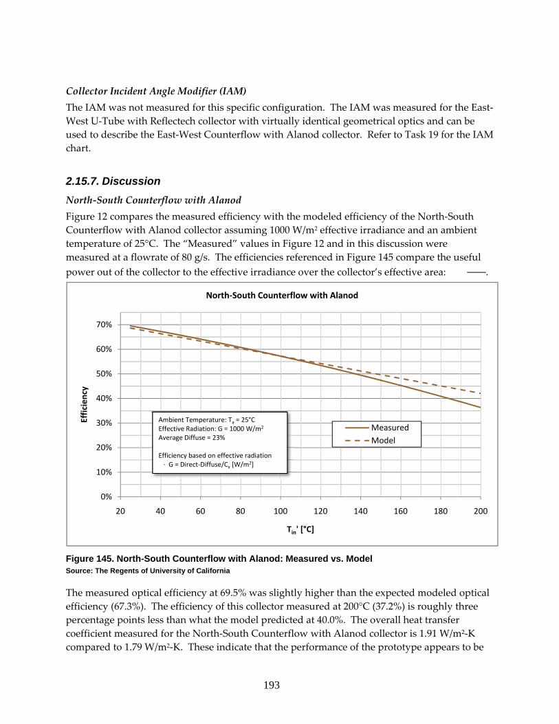
193
Collector Incident Angle Modifier (IAM) The IAM was not measured for this specific configuration. The IAM was measured for the East‐West U‐Tube with Reflectech collector with virtually identical geometrical optics and can be used to describe the East‐West Counterflow with Alanod collector. Refer to Task 19 for the IAM chart.
2.15.7. Discussion North‐South Counterflow with Alanod Figure 12 compares the measured efficiency with the modeled efficiency of the North‐South Counterflow with Alanod collector assuming 1000 W/m2 effective irradiance and an ambient temperature of 25°C. The “Measured” values in Figure 12 and in this discussion were measured at a flowrate of 80 g/s. The efficiencies referenced in Figure 145 compare the useful power out of the collector to the effective irradiance over the collector’s effective area: .
Figure 145. North-South Counterflow with Alanod: Measured vs. Model Source: The Regents of University of California
The measured optical efficiency at 69.5% was slightly higher than the expected modeled optical efficiency (67.3%). The efficiency of this collector measured at 200°C (37.2%) is roughly three percentage points less than what the model predicted at 40.0%. The overall heat transfer coefficient measured for the North‐South Counterflow with Alanod collector is 1.91 W/m2‐K compared to 1.79 W/m2‐K. These indicate that the performance of the prototype appears to be
0%
10%
20%
30%
40%
50%
60%
70%
20 40 60 80 100 120 140 160 180 200
Efficiency
Tin' [°C]
North‐South Counterflow with Alanod
MeasuredModel
Ambient Temperature: Ta = 25°CEffective Radiation: G = 1000 W/m2
Average Diffuse = 23%
Efficiency based on effective radiation∙ G = Direct‐Diffuse/Cx [W/m2]

194
slightly less than what the model predicted. Overall, the measurements of the optical and thermal efficiency appear to have a very good agreement with the model. As seen in Figure 6, the acceptance angle of the North‐South Counterflow with Alanod collector was found to be +/‐ 55 degrees as opposed to the designed +/‐ 60 degrees which suggests that the optics of the system are not exactly as designed. One possible defect is the shape of the reflector is not accurate. A more likely reason for the lowered acceptance angle is that the placement of the absorber may not have been in the designed position. If the absorber is lower than the designed position then the acceptance angle will be lowered while also increasing the optical efficiency at normal incidence which may also explain the higher than expected optical efficiency. This could happen if either the glass tubes’ placement in the frame’s holes were off or the absorber in the glass tube was not exactly concentric. In addition to a lower than predicted acceptance angle, the IAM chart seems to be off center. The fact that the measurements were done continuously throughout the day, the shift in the chart is likely due to a thermal constant. Efficiencies based on DNI in Figures 4 and 5 appear very high. These high efficiencies are due to the fact that this collector was tested when there was a relatively large percentage of diffuse light. During the testing of this collector, the percent diffuse ranged between 15% and 30% with an average of 23%.
East‐West Counterflow with Alanod Figure 13 compares the measured efficiency with the modeled efficiency of the North‐South Counterflow with Alanod collector assuming 1000 W/m2 effective irradiance and an ambient temperature of 25°C. The “Measured” values in Figure 13 and in this discussion were measured at a flowrate of 80 g/s. The efficiencies referenced in Figure 13 compare the useful power out of the collector to the effective irradiance over the collector’s effective area: .
The optical efficiency value used for the measured chart was an assumed value of 64.6%. Since the least squared quadratic curve has a natural shape, the assumed optical efficiency appears to fit the rest of the data. The measured efficiency at 200°C in Figure 13 is 40% compared to the model efficiency of 47.4%. The overall heat transfer coefficient measured for the collector and the model were 1.39 W/m2‐K and 1.17 W/m2‐K respectively. The thermal efficiency of the East‐West Counterflow with Alanod collector appears to suffer from more heat loss than what was expected from the model. This lower efficiency is likely, in part, due to a high thermal resistance in the counterflow tubes. This high resistance and the higher concentration ratio of the East‐West collector would allow the absorber temperature to be much higher than the oil temperature resulting in a large radiative loss from the absorber. In addition, the efficiency curve in Figure 13 is nearly linear which suggests that there is a large portion of the heat loss that is not due to radiation and can be assumed to be from losses in the manifold insulation.

195
Figure 146 East-West Counterflow with Alanod: Measured vs. Model Source: The Regents of University of California
Efficiencies based on effective irradiance in Figure 8 are roughly 9% lower than the efficiencies based on DNI in Figure 10 for this East‐West collector. With an average diffuse of 15% during testing and a concentration of 1.8, one would expect an 8% difference in the efficiency between DNI and effective irradiance. The amount of diffuse accepted by the collector appears to agree with factor in the effective irradiance calculations. Comparison Figure 14 and Table compares the efficiencies of the North‐South and the East‐West Counterflow with Alanod collectors. As expected, the North‐South version has a higher optical efficiency. The North‐South collector outperformed the East‐West collector from temperatures up to 150°C while the model suggests that the East‐West collector should have a higher efficiency starting at about 85°C. As stated earlier, the East‐West collector likely suffered from a large thermal resistance in the absorber and manifold heat losses which contributed to its lowered efficiency. Table 38: Comparison of the North-South and East-West Counterflow with Alanod collectors
G=GRabl G=GDNI North-South East-West North-South East-West
Optical Efficiency 69.5% 64.6% 87.7% 69.3% Efficiency at 100 °C 57.2% 54.6% 73.7% 59.9% Efficiency at 200 °C 36.3% 40.3% 53.3% 44.3%
Loss coefficient (1) 1.445 W/m2-K 1.293 W/m2-K 1.793 W/m2- 1.139 W/m2-
0%
10%
20%
30%
40%
50%
60%
70%
20 40 60 80 100 120 140 160 180 200
Efficiency
Tin' [°C]
East‐West Counterflow with Alanod
Measured
Model
Ambient Temperature: Ta = 25°CEffective Radiation: G = 1000 W/m2
Average Diffuse = 15%
Efficiency based on effective radiation∙ G = Direct‐Diffuse/Cx [W/m2]
Optical Efficiency for the measured curve is an assumed value.

196
G=GRabl G=GDNI North-South East-West North-South East-West
K K Loss coefficient (2) .00323 W/m2-
K2 0.0007 W/m2-
K2 .0045 W/m2-
K2 .0021 W/m2-
K2 Overall heat loss
coefficient 1.910 W/m2-K 1.393 W/m2-K 1.973 W/m2-
K 1.436 W/m2-
K Acceptance angle11 +/- 55° +/- 32.5° +/- 55° +/- 32.5°
Source: The Regents of University of California
Another possible source of error is the fact that two different methods of assuming the heat capacity of the oil were employed. The measurements used to determine the heat capacity of the oil that were used for the North‐South calculations were lower than the table values from the oil manufacturer that were used for the East‐West calculations. If the same values for the heat capacity were used, it is likely that the East‐West collector would look additionally worse compared to the North‐South collector.
Figure 147. Counterflow Efficiencies: North-South vs. East-West Source: The Regents of University of California
11 The acceptance angle of the East-West Counterflow Alanod collector can be assumed to be the same as the U-Tube Reflectech version as presented in the table.
0%
10%
20%
30%
40%
50%
60%
70%
20 40 60 80 100 120 140 160 180 200
Efficiency
Tin' [°C]
XCPC Efficiencies: Counterflow Tubes
East‐West CF‐Tube Alanod
North‐South CF‐Tube Alanod
Ambient Temperature: Ta = 25°CEffective Radiation: G = 1000 W/m2
Efficiency based on effective radiation∙ G = Direct‐Diffuse/Cx [W/m2]
Optical Efficiency for the EW curve is an assumed value.

197
Possible errors Errors in the data may come from any of the following: instrumental errors, measurement errors, assumed values, tolerance errors, environmental effects, ground reflection, and errors in theory.
Although calibrated, instruments such as pyranometers, pyrheliometers, thermocouples and other temperature sensors, the flowmeter, and data acquisition systems may have non‐trivial errors associated with them. While steps were taken to minimize these sources of error, it is impossible to avoid them completely. Errors in any of these instruments would affect the efficiency measurements and/or the temperature scale.
The effective area of the collector is a possible source of error due to it being measured manually but this error should be less than a fraction of a percent. Any error in the area of the collector would directly affect the calculated efficiency values.
Material properties of the oil, absorber, glass, and reflector may differ from the model. The heat capacity values used for the heat transfer oil (Duratherm 600) were measured by an outside source (Rose Consulting) with their own set of possible errors. The lab that measured the heat capacity of the oil estimated the error to be as high as 2%. Any error in the heat capacity would directly affect the calculated efficiency values. Any differences in the properties of the reflector, glass, or absorber would create an error in estimating the optical and thermal efficiencies.
The shape of the reflector and the position of the holes in the frame are subject to tolerance errors that would affect the optical efficiency and the acceptance angle.
Soiling of the reflectors and the glass tubes can have a negative effect on the optical efficiency.
Ground reflection is inevitable when testing solar thermal collectors outdoors. The amount of ground reflection available to the collector depends on the optics and orientation of the collector, the time of day and the position of the tracker. While the pyranometer mounted on the tracker should be able to detect all or most of the ground reflection, the angle of incidence may be too severe to be accepted by the collector. Collectors with lower concentrations and collectors oriented in a vertical position like the North‐South collectors will be able to accept more of this reflected radiation. The ground reflection will be treated as diffuse light. Ground reflection can cause variation in data and cause East‐West collectors to have an apparent lower than expected performance.
Much of the data presented in this report uses an effective irradiance to represent the amount of available power to the collector. The effective irradiance adjustment attempts to take into account that a concentrating optical system cannot accept all of the diffuse and is therefore not considered in the efficiency. Using this method will favor collectors with larger concentration ratios
198
Other data is presented in this report uses the direct normal irradiance (DNI) to represent the incoming radiation. This method completely ignores diffuse radiation which favors collectors with low concentrations. Using this method with data having a large percent of the irradiance as diffuse can create apparently high efficiencies.
Since the testing was done outdoors, it is virtually impossible to test with a constant or consistent ambient temperature. The charts and the data presented in this report attempt to minimize the effect of the differences in the ambient temperature by presenting data with the reduced temperature. Unfortunately, these evacuated tube collectors primarily lose heat through radiation which is non‐linear. In addition, the emissivity of the absorber is a function of the absorber temperature only and not of the ambient temperature. This creates a less than perfect correction for the ambient temperature which is most apparent when a collector was tested during very different outdoor temperatures or when comparing two different collectors that were tested in different seasons.
2.16. Task 17 In this task the contractor compared the test results for optical and thermal collector efficiency obtained in Task 16 with the expected optical and thermal efficiency predicted by models that were originally developed in Task 5 and further improved in the course of this Task. The comparison applies to the XCPC collector named “Metal absorber with glass‐to‐metal seal – North‐South orientation.” The detailed design and the specifications of this XCPC have been described in the Task 12 Report. The tested collector consisted of 6 absorber tubes.

199
Figure 148. Shows the comparison between expectations from modeling with achieved test results.
Source: The Regents of University of California
Figure 149. Comparison of measured and modeled collector efficiency Source: The Regents of University of California
30%
35%
40%
45%
50%
55%
60%
65%
70%
25 50 75 100 125 150 175 200
Efficiency
Tinlet [°C]
Efficiency of Eurocon North‐South(based on irradiance measured on collector plane according to Ari Rabl
Flow rate 80 g/s; assuming Tambient = 25°C and GRabl = 1,000 W/m2 (with GRabl = Gdirect + Gdiffuse/C)
Model
Measured

200
The comparison shows that the measured optical efficiency is very close to expectations, namely around 65%. This indicates that the manufacturing of the external reflectors and the alignment of the absorber tubes relative to the reflectors are well done.
There is a shortfall of measured thermal efficiency relative to the model at higher temperatures. The contractor has two explanations for that: First, the model does not consider the heat losses in the manifold. The manifold has been insulated well, but such insulation can never be perfect. Secondly, the absorber tube uses a cylindrical metal fin absorber that is welded just along one fine line onto the counter‐flow heat exchanger that carries the heat transfer fluid (Figure 149). The thermal contact between the cylindrical metal fin absorber and the counter‐flow tube is believed to constitute the limiting factor in heat transfer and thus the thermal performance of the absorber tube.
Figure150. Schematic of absorber tube used in tested XCPC
Source: The Regents of University of California
An improved version of the XCPC with a U‐tube heat exchanger instead of the counter‐flow heat exchanger will be manufactured and tested in the next project tasks. This U‐tube version is expected to have better heat transfer and thus thermal efficiency than the version with the counter‐flow tube, because there will be two connection lines between absorber fin and metal tube instead of one. An additional advantage of the new version will be that the aluminum absorber fin will be made out of extruded aluminum instead of using an aluminum foil. The extruded absorber fin will have better mechanical stability than the foil. A schematic drawing of the improved version of the XCPC is shown in Figure 150.
Absorber fin (extruded Al)
Glass

201
2.17. Task 18 Test plan to test the performance of the XCPC prototype The following test plan is based on the international standard for solar thermal collector testing, ISO 9806‐1 (Part 1). Some modifications have been made to account for the specific design, namely a stationary concentrating evacuated tube collector, and the temperature range of operation, which is up to 450°F. The tests to be performed in Task 19 will include:
• Collector time constant • Collector thermal efficiency • Collector optical efficiency • Collector incident angle modifier • Pressure drop across the collector
Description of Test Loop The test facility uses is a closed loop system that includes a circulating oil temperature controller with integrated pump and expansion tank (see Figure 151). The circulating oil temperature controller provides a selectable constant temperature (up to 500°F) to the heat transfer fluid that is circulated through the collector. The loop further includes a flow meter, temperature sensors before and after the collector, and a calorimeter. The calorimeter is described in detail below. The solar collector is mounted on a dual axis tracker to allow the measurement of collector performance under controlled incidence angles. The test facility further includes a meteorological station with a Precision Spectral Pyranometer that is mounted on the same tracker as the solar collector, a Normal Incidence Pyrheliometer mounted on a separate dual‐axis tracker, a thermometer to measure the ambient temperature, and an anemometer.

202
Figure 151. Schematic of Test Facility Source: The Regents of University of California
exchanger
~1 gpm U-tube heat
Temperature Control System ½ “ NPT Cooling Water Outlet ½ “ NPT Cooling Water Inlet 1 ½” NPT Oil Outlet 30 gpm 1 ½” NPT Oil Inlet Distance ~15 foot
CMXO Circulating Oil
Flexible pipe Sun
Tracker (Moving
Structure) Chromalox
6 kW 500°F Flexible pipe
Heater
30 gpm 6 kW
Expansion Tank Pump oling
module
Co
1a
b
1
2 3 5 4
tor(s) 6a
collec
2 kW Calorimeter
6b Solar
6d
1c
6c
1abc Gate valves 2 Diverter valve 3 (Back)pressure regulating valve 4 Flow control valve 5 Flow meter 6abcd Temperature sensors

203
The data from the flow meter, the temperature sensors and the meteorological station are recorded through a data acquisition system. Instrumentation Circulating oil temperature controller: Chromalox CMXO 6kW (with integrated pump and expansion tank) Temperature sensors: Type‐K thermocouples from Omega Flow meter: Micro Motion Coriolis F‐Series sensor Flow control valve: Valtek ½” Flow Top Control Valve Back pressure regulating valve: Jordan: 1” 50‐100‐S6‐I5‐S6‐Y‐8‐21‐S6‐MD Pressure Control Valve Sun tracker: Wattsun AZ‐125 dual axis tracker Calorimeter: Custom made by Valin Inc. Pyranometer: Eppley Precision Spectral Pyranometer Pyrheliometer: Eppley Normal Incidence Pyrheliometer Amplifiers: Agilent 34970A Data Acquisition/Switch Unit Data logger: Obvius A8811 and A8923 Test Procedure for Collector Time Constant Testing will be performed outdoors with a solar irradiance on the plane of the collector aperture greater than 800 W/m2. The heat transfer fluid will be circulated through the collector at the same flow rate as used during collector thermal efficiency testing. Initially the collector’s aperture will be shielded from solar radiation by means of a solar‐reflecting cover, and the temperature of the heat transfer fluid at the collector inlet will be approximately equal to the ambient air temperature. When a steady state has been reached, the cover will be removed and measurements of the collector fluid inlet temperature (tin), the collector fluid outlet temperature (te), and the surrounding air temperature (ta) will be taken until steady‐state conditions have been reached again. A steady state condition is assumed to exist when the outlet temperature of the fluid varies by less than 0.05°C per minute. The difference between the temperature of the fluid at the collector outlet and that of the surrounding air will be measured against time, beginning with the initial steady‐state condition and continuing until the second steady state has been achieved at a higher temperature (see Figure 152). The time constant of the collector is defined as the time taken for the collector outlet temperature to rise by 63.2% of the total increase from
to following the step increase in solar irradiance at time zero.
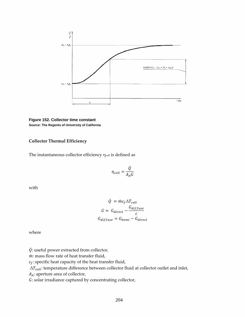
204
Figure 152. Collector time constant Source: The Regents of University of California
Collector Thermal Efficiency The instantaneous collector efficiency ηcoll is defined as
with
Δ
where
: useful power extracted from collector, : mass flow rate of heat transfer fluid, : specific heat capacity of the heat transfer fluid,
Δ : temperature difference between collector fluid at collector outlet and inlet, : aperture area of collector, : solar irradiance captured by concentrating collector,

205
: direct normal irradiance (measured with a pyrheliometer), : diffuse sky irradiance,
: hemispherical irradiance (measured with a pyranometer). c : geometric concentration of collector The determination of the instantaneous collector efficiency based on the formula above requires the measurement of the mass flow rate of heat transfer fluid, the temperature difference between the heat transfer fluid at the collector outlet and inlet, the aperture area of collector, the solar irradiance, and the knowledge of the specific heat capacity of the heat transfer fluid (at various temperatures). Efficiency Measurement with Calorimeter The instantaneous collector efficiency ηcoll has been defined above as
Δ
If one prefers not to rely on the measurement accuracy of and the accuracy of the tabulated values of the heat capacity of the heat transfer medium, an alternative approach can be used to determine . This is by using a calorimeter, which is a perfectly insulated electric heater placed in series after the solar collector. In this case, the heat loss of the calorimeter is assumed to be zero, and the useful power extracted from the calorimeter is equal to the electric power consumption of the calorimeter, which can be measured very accurately. With
· · ∆ ,
and assuming that the values of and are approximately equal in the collector and in the calorimeter, the product can be replaced by:
·∆
,
where
: useful power extracted from collector (= power consumption of calorimeter); Δ calorimeter: temperature difference of fluid between calorimeter outlet and inlet.

206
Thus, the instantaneous collector efficiency becomes:
· · ΔΔ
.
The determination of the instantaneous collector efficiency based on the method using a colorimeter requires the measurement of the temperature difference of the heat transfer fluid at the collector outlet and inlet, the temperature difference of the heat transfer fluid at the calorimeter outlet and inlet, the aperture area of collector, and the solar irradiance. It is not necessary to measure the mass flow rate of heat transfer fluid and to know the specific heat capacity of the heat transfer fluid. Temperature dependence of collector efficiency
The temperature dependence of the instantaneous efficiency can be represented graphically as a function of the reduced temperature difference (see Figure 153). The thermal performance of the collector can then be characterized by the two coefficients and , which are determined by a least square parabolic curve fit:
with η0: optical efficiency : reduced temperature difference
where : ambient temperature, : collector inlet temperature, and : coefficients determined from least squares parabolic curve fit,
and the value of in the formula above is assumed to be 800 ⁄ .

207
Figure 153. Example of a collector efficiency vs. temperature curve Source: The Regents of University of California
Collector optical efficiency The optical efficiency of the collector will be determined using the same test procedure as for the thermal efficiency tests (as described above), only that the temperature of the heat transfer fluid at the collector inlet will be kept equal to the ambient temperature. In this case the calculated thermal efficiency is equal to the optical efficiency (no heat loss). Collector incident angle modifier The collector incident angle modifier (IAM) will be determined by measuring the optical efficiency (as described above) under variation of the incidence angle between the sunlight and the collector plane. Pressure drop across the collector The pressure drop across the collector will be measured by comparing the difference in the pressure of the heat transfer fluid after and before the collector. The pressure drop measurements will be made for different temperatures between ambient and 400°F.
2.18. Task 19 The goal of this task was to test the improved XCPCs per the test plan outlined in Task 18. The tests include: instantaneous thermal efficiency, optical efficiency, incidence angle modifier, and stagnation.

208
2.18.1. Tested Collectors In this task the contractor tested the following XCPC versions:
U‐Tube with Alanod Reflectors in North‐South orientation
U‐Tube with Alanod Reflectors in East‐West orientation
X‐Tube with Alanod Reflectors in East‐West orientation
U‐Tube with Reflectech Reflectors in North‐South orientation
U‐Tube with Reflectech Reflectors in East‐West orientation
The detailed design and the specifications of these XCPCs have been described in the Task 17 Report. Both tested collectors consisted of 6 absorber tubes each.
2.18.2. Collector Thermal Efficiency: Method 1 The instantaneous collector efficiency ηcoll is defined as
with
Δ ,
,
Where
: useful power extracted from collector,
: mass flow rate of heat transfer fluid,
: specific heat capacity of the heat transfer fluid,
Δ : temperature difference between collector fluid at collector outlet and inlet,
: effective aperture area of collector – we define this area as the length of the active area of the absorber tube (which is the area covered by the selective coating) times the width of the reflector
: solar irradiance captured by concentrating collector,
: direct normal irradiance (measured with a pyrheliometer),
: diffuse sky irradiance,
: hemispherical irradiance (measured with a pyranometer).

209
: geometric concentration of collector
2.18.3. Collector Thermal Efficiency: Method 2 The instantaneous collector efficiency ηcoll can be defined as
with
·ΔΔ
,
,
Where
: useful power extracted from collector,
: calorimeter power,
Δ : temperature difference between collector fluid at collector outlet and inlet,
Δ : temperature difference between the fluid at the calorimeter outlet and inlet,
: effective aperture area of collector – we define this area as the length of the active area of the absorber tube (which is the area covered by the selective coating) times the width of the reflector
: solar irradiance captured by concentrating collector,
: direct normal irradiance (measured with a pyrheliometer),
: diffuse sky irradiance,
: hemispherical irradiance (measured with a pyranometer).
: geometric concentration of collector
2.18.4. Temperature dependence of collector efficiency The temperature dependence of the instantaneous efficiency can be represented graphically as a function of the reduced temperature . The thermal performance of the collector can then be characterized by the two coefficients and , which are determined by a least square parabolic curve fit:
with

210
: optical efficiency
: reduced temperature
where
: ambient temperature,
: collector inlet temperature,
and : coefficients determined from least squares parabolic curve fit, and the value of in the formula above is assumed to be 1000 / .
2.18.5. Description of Test Loop The test facility used is a closed loop system that includes a circulating oil temperature controller with integrated pump and expansion tank (see Fig. 1). The circulating oil temperature controller provides a selectable constant temperature (up to 500°F) to the heat transfer fluid that is circulated through the collector. The loop further includes a flow meter and temperature sensors before and after the collector. There are flow mixers introduced into the loop before each temperature sensor. The solar collector is mounted on a dual axis tracker to allow the measurement of collector performance under controlled incidence angles.
The test facility further includes a meteorological station with a Precision Spectral Pyranometer and a Normal Incidence Pyrheliometer that are both mounted on the same tracker as the solar collector, a thermometer to measure the ambient temperature, and an anemometer.
In addition, a calorimeter was used as an improved method of determining the instantaneous thermal efficiency without depending on knowing the heat capacity of the oil12. XXX
12 The U-Tube with Alanod Reflectors in North-South configuration collector was not tested using this method.

211
Figure 154. Schematic of Test Facility Source: The Regents of University of California
Distance ~15 foot
1 ½” NPT Oil Inlet
30 gpm
1 ½” NPT Oil Outlet
½ “ NPT Cooling Water Inlet
½ “ NPT Cooling Water Outlet
Chromalox CMXO Circulating Oil Temperature Control System
Sun Tracker (Moving Structure)
Flex pipe
Flexible pipe 6 kW Heater
Pump 30 gpm
Expansion Tank
Cooling module
1a
1b
2
3
4 5 6a
Solar collector(s)
6b 2 kW Calorimeter 6
d
1c
6c
1abc Gate valves 2 Diverter valve 3 (Back)pressure regulating valve 4 Flow control valve 5 Flow meter 6abcd Temperature sensors

212
The data from the flow meter, the temperature sensors and the meteorological station were recorded through a data acquisition system.
2.18.6. Instrumentation Circulating oil temperature controller: Chromalox CMXO 6kW (with integrated pump
and expansion tank)
Temperature sensors: Type‐K thermocouples from Omega
Flow meter: Micro Motion Coriolis F‐Series sensor
Flow control valve: Valtek ½” Flow Top Control Valve
Back pressure regulating valve: Jordan: 1” 50‐100‐S6‐I5‐S6‐Y‐8‐21‐S6‐MD
Pressure Control Valve
Sun tracker: Wattsun AZ‐125 dual axis tracker
Calorimeter: Custom made by Valin Inc.
Pyranometer: Eppley Precision Spectral Pyranometer
Pyrheliometer: Eppley Normal Incidence Pyrheliometer
Data Acquisition System 1: Agilent 34970A Data Acquisition/Switch Unit
Data Acquisition System 2: Acquisuite Data Acquisition System
2.18.7. Test Results of “U-Tube with Alanod Reflectors in North-South orientation”
Collector description Table 39. Collector Description of North-South U-Tube with Alanod Collector
Orientation North-South Concentration 1.15
Effective Collector Area 2.076 m2 Tube Type U-Tube
Number of Tubes 6 Reflector Alanod (90%)
Source: The Regents of University of California

213
Collector optical efficiency The optical efficiency of the North‐South Counterflow with Alanod collector was used as an assumed value of the optical efficiency of the North‐South U‐Tube with Alanod since the geometry and optical properties of the system were assumed to be unchanged.
The optical efficiency based on an effective irradiance ( / ) was assumed to be 69.1%. The optical efficiency based on direct normal irradiance ( was assumed to be 79.3%.
Collector thermal efficiency The efficiency of the XCPC was measured from 6/30 ‐ 7/3/08 using “Method 1” at the following collector inlet temperatures: 80°C, 100°C, 120°C, 140°C, 160°C, 180°C, and 200°C; and at the following flow rates: 80 g/s, 100 g/s, 120 g/s, and 140 g/s.
The heat capacity of the oil was measured in August 2008 using the calorimeter during the East‐West U‐Tube with Alanod tests. A linear approximation to the measurements was used to calculate the efficiency of the collector: 0.00489 · 1.815.
The performance characteristics are tabulated in Table 2 and the collector efficiencies are depicted in
Figure 1 through Figure 158. Figure 3 and Figure 7 are derived from Figure 2 and Figure 4 respectively by assuming an ambient temperature of 25°C and an effective insolation of 1,000 W/m2 that is captured by the XCPC. Figures 2 and 3 display the efficiencies based on the effective irradiance while Figures 4 and 5 display the efficiencies based on the direct normal irradiance (DNI) .
Table 40. Performance Characteristics of North-South U-Tube with Alanod Collector
G=GE G=GDNI Optical Efficiency 69.1% 79.3% Efficiency at 100 °C 58.5% 69.3% Efficiency at 200 °C 36.4% 36.4%
Loss coefficient (1) 1.080 W/m2-K 0.595 W/m2-K Loss coefficient (2) 0.00351 W/m2-
K2 0.00993 W/m2-
K2 Overall heat loss coefficient 1.891 W/m2-K 2.382 W/m2-K
Source: The Regents of University of California
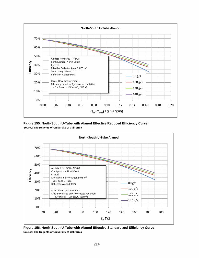
214
Figure 155. North-South U-Tube with Alanod Effective Reduced Efficiency Curve Source: The Regents of University of California
Figure 156. North-South U-Tube with Alanod Effective Standardized Efficiency Curve Source: The Regents of University of California
0%
10%
20%
30%
40%
50%
60%
70%
0.00 0.02 0.04 0.06 0.08 0.10 0.12 0.14 0.16 0.18 0.20
Efficiency
(Tin ‐ Tamb) / G [m2 °C/W]
North‐South U‐Tube Alanod
80 g/s
100 g/s
120 g/s
140 g/s
All data from 6/30 ‐ 7/3/08Configuration: North‐SouthCx=1.15Effective Collector Area: 2.076 m2
Tube: Jiang U‐TubeReflector: Alanod(90%)
Direct Flow measurementsEfficiency based on Cx‐corrected radiation‐ G = Direct ‐ Diffuse/Cx [W/m2]
0%
10%
20%
30%
40%
50%
60%
70%
20 40 60 80 100 120 140 160 180 200
Efficiency
Tin [°C]
North‐South U‐Tube Alanod
80 g/s
100 g/s
120 g/s
140 g/s
All data from 6/30 ‐ 7/3/08Configuration: North‐SouthCx=1.15Effective Collector Area: 2.076 m2
Tube: Jiang U‐TubeReflector: Alanod(90%)
Direct Flow measurementsEfficiency based on Cx‐corrected radiation‐ G = Direct ‐ Diffuse/Cx [W/m2]

215
Figure 157. North-South U-Tube with Alanod Direct Reduced Efficiency Curve Source: The Regents of University of California
Figure 158. North-South U-Tube with Alanod Direct Standardized Efficiency Curve Source: The Regents of University of California
0%
10%
20%
30%
40%
50%
60%
70%
80%
0.00 0.02 0.04 0.06 0.08 0.10 0.12 0.14 0.16 0.18 0.20
Efficiency
(Tin ‐ Tamb) / G [m2 °C/W]
North‐South U‐Tube Alanod (DNI)
80 g/s
100 g/s
120 g/s
140 g/s
All data from 6/30 ‐ 7/3/08Configuration: North‐SouthCx=1.15Effective Collector Area: 2.076 m2
Tube: Jiang U‐TubeReflector: Alanod(90%)
Direct Flow measurementsEfficiency based on Direct Normal Irradiance‐ G = GDNI
0%
10%
20%
30%
40%
50%
60%
70%
80%
20 40 60 80 100 120 140 160 180 200
Efficiency
Tin [°C]
North‐South U‐Tube Alanod (DNI)
80 g/s
100 g/s
120 g/s
140 g/s
All data from 6/30 ‐ 7/3/08Configuration: North‐SouthCx=1.15Effective Collector Area: 2.076 m2
Tube: Jiang U‐TubeReflector: Alanod(90%)
Direct Flow measurementsEfficiency based on Direct Normal Irradiance‐ G = GDNI

216
Collector Incident Angle Modifier (IAM) The incident angle modifier (IAM) was not measured for this specific configuration. Since IAM is almost completely dependent on the geometric shape of the reflector and the placement of the tubes, it is reasonable to use the previously measured IAM to describe this collector.
2.18.8. Test Results of “U-Tube with Alanod Reflectors in East-West orientation”
Collector description Table 41. Description of East-West U-Tube with Alanod Collector
Orientation East-West Concentration 1.80
Effective Collector Area 3.24 m2 Tube Type U-Tube
Number of Tubes 6 Reflector Alanod (90%)
Source: The Regents of University of California
Collector optical efficiency The optical efficiency of the East‐West U‐Tube with Alanod collector was assumed to be the value taken from a linear extrapolation.
The optical efficiency based on an effective irradiance ( / ) was assumed to be 66.4%. The optical efficiency based on direct normal irradiance ( was assumed to be 71.5%.
Collector thermal efficiency The efficiency of the XCPC was measured from 8/13 – 8/27/08 using “Method 1” ” and “Method 2” at the following collector inlet temperatures: 80°C, 100°C, 120°C, 140°C, 160°C, 180°C, and 200°C; and at the following flow rates: 80 g/s, 100 g/s, 120 g/s, 140 g/s, and 160 g/s. All efficiencies reported are based on “Method 2.”
The performance characteristics are tabulated in Table 4 and the collector efficiencies are depicted in Figure 6 through Figure 9. Figure 7 and Figure 9 are derived from Figure 6 and Figure 8 respectively by assuming an ambient temperature of 25°C and an effective insolation of 1,000 W/m2 that is captured by the XCPC. Figures 6 and 7 display the efficiencies based on the effective irradiance while Figures 8 and 9 display the efficiencies based on the direct normal irradiance (DNI) .

217
Table 42. Performance Characteristics of East-West U-Tube with Alanod Collector Source: The Regents of University of California
G=GE G=GDNI Optical Efficiency 66.4% 71.5% Efficiency at 100 °C 58.3% 63.1% Efficiency at 200 °C 43.2% 45.2%%
Loss coefficient (1) 0.908 W/m2-K 0.822 W/m2-K Loss coefficient (2) 0.00239 W/m2-
K2 0.00387 W/m2-
K2 Overall heat loss coefficient 1.339 W/m2-K 1.519 W/m2-K
Figure 159. East-West U-Tube with Alanod Effective Reduced Efficiency Curve Source: The Regents of University of California
0%
10%
20%
30%
40%
50%
60%
70%
0.00 0.02 0.04 0.06 0.08 0.10 0.12 0.14 0.16 0.18 0.20
Efficiency
(Tin ‐ Tamb) / G [m2 °C/W]
East‐West U‐Tube Alanod
80 g/s
100 g/s
120 g/s
140 g/s
All data from 8/13 ‐ 8/27/08Configuration: East‐WestCx=1.80Effective Collector Area: 3.24 m2
Tube: Jiang U‐TubeReflector: Alanod(90%)
Calorimetry measurementsEfficiency based on Cx‐corrected radiation‐ G = Direct ‐ Diffuse/Cx [W/m2]

218
Figure 160. East-West U-Tube with Alanod Effective Standardized Efficiency Curve Source: The Regents of University of California
Figure 161. East-West U-Tube with Alanod Direct Reduced Efficiency Curve Source: The Regents of University of California
0%
10%
20%
30%
40%
50%
60%
70%
20 40 60 80 100 120 140 160 180 200
Efficiency
Tin [°C]
East‐West U‐Tube Alanod
80 g/s
100 g/s
120 g/s
140 g/s
All data from 8/13 ‐ 8/27/08Configuration: East‐WestCx=1.80Effective Collector Area: 3.24 m2
Tube: Jiang U‐TubeReflector: Alanod(90%)
Calorimetry measurementsEfficiency based on Cx‐corrected radiation‐ G = Direct ‐ Diffuse/Cx [W/m2]
0%
10%
20%
30%
40%
50%
60%
70%
80%
0.00 0.02 0.04 0.06 0.08 0.10 0.12 0.14 0.16 0.18 0.20
Efficiency
(Tin ‐ Tamb) / G [m2 °C/W]
East‐West U‐Tube Alanod (DNI)
80 g/s
100 g/s
120 g/s
140 g/s
All data from 7/1 ‐ 9/16/09Configuration: East‐WestCx=1.80Effective Collector Area: 3.24 m2
Tube: Jiang U‐TubeReflector: Reflectech (94%)
Calorimetry measurementsEfficiency based on Direct Normal Irradiance‐ G = GDNI

219
Figure 162. East-West U-Tube with Alanod Direct Standardized Efficiency Curve Source: The Regents of University of California
Collector Incident Angle Modifier (IAM) The incident angle modifier (IAM) was not measured for this specific configuration. Since IAM is almost completely dependent on the geometric shape of the reflector and the placement of the tubes, it is reasonable to use the measured IAM from the U‐Tube with Reflectech Reflectors in East‐West collector to describe this collector.
2.18.9. Test Results of “X-Tube with Alanod Reflectors in East-West orientation”
Collector description Table 43. Description of East-West Counterflow with Alanod Collector
Orientation East-West Concentration 1.80
Effective Collector Area 3.1 m2 Tube Type X-Tube
Number of Tubes 6 Reflector Alanod (90%)
Source: The Regents of University of California
0%
10%
20%
30%
40%
50%
60%
70%
80%
20 40 60 80 100 120 140 160 180 200
Efficiency
Tin [°C]
East‐West U‐Tube Alanod (DNI)
80 g/s
100 g/s
120 g/s
140 g/s
All data from 8/13 ‐ 8/27/08Configuration: East‐WestCx=1.80Effective Collector Area: 3.24 m2
Tube: Jiang U‐TubeReflector: Alanod(90%)
Calorimetry measurementsEfficiency based on Direct Normal Irradiance‐ G = GDNI

220
Collector optical efficiency The optical efficiency of the East‐West X‐Tube with Alanod collector was assumed to be the value taken from a linear extrapolation.
The optical efficiency based on an effective irradiance ( / ) was assumed to be 68.6%. The optical efficiency based on direct normal irradiance ( was assumed to be 75.0%.
Collector thermal efficiency The efficiency of the XCPC was measured from 9/18 – 10/13/08 using “Method 1” ” and “Method 2” at the following collector inlet temperatures: 80°C, 100°C, 120°C, 140°C, 160°C, 180°C, and 200°C; and at the following flow rates: 80 g/s, 100 g/s, 120 g/s, 140 g/s, and 160 g/s. All efficiencies reported are based on “Method 2.”
The performance characteristics are tabulated in Table 6 and the collector efficiencies are depicted in Figure 10 through Figure 13. Figure 11 and Figure 13 are derived from Figure 10 and Figure 12 respectively by assuming an ambient temperature of 25°C and an effective insolation of 1,000 W/m2 that is captured by the XCPC. Figures 10 and 11 display the efficiencies based on the effective irradiance while Figures 12 and 13 display the efficiencies based on the direct normal irradiance (DNI) .
Table 44. Performance Characteristics of East-West X-Tube with Alanod Collector
G=GE G=GDNI Optical Efficiency 68.6% 75.0% Efficiency at 100 °C 59.9% 65.9% Efficiency at 200 °C 39.9% 43.4%
Loss coefficient (1) 0.799 W/m2-K 0.799 W/m2-K Loss coefficient (2) 0.00481 W/m2-
K2 0.00481 W/m2-
K2 Overall heat loss coefficient 1.664 W/m2-K 1.838 W/m2-K
Source: The Regents of University of California
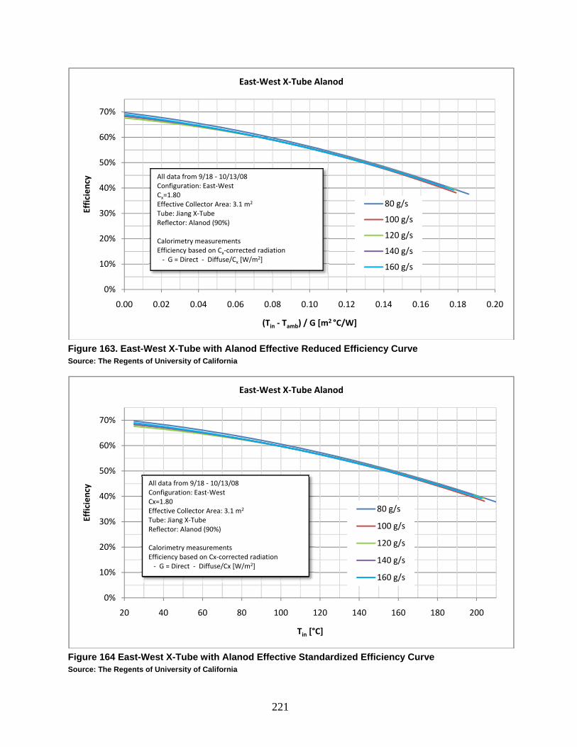
221
Figure 163. East-West X-Tube with Alanod Effective Reduced Efficiency Curve Source: The Regents of University of California
Figure 164 East-West X-Tube with Alanod Effective Standardized Efficiency Curve Source: The Regents of University of California
0%
10%
20%
30%
40%
50%
60%
70%
0.00 0.02 0.04 0.06 0.08 0.10 0.12 0.14 0.16 0.18 0.20
Efficiency
(Tin ‐ Tamb) / G [m2 °C/W]
East‐West X‐Tube Alanod
80 g/s
100 g/s
120 g/s
140 g/s
160 g/s
All data from 9/18 ‐ 10/13/08Configuration: East‐WestCx=1.80Effective Collector Area: 3.1 m2
Tube: Jiang X‐TubeReflector: Alanod (90%)
Calorimetry measurementsEfficiency based on Cx‐corrected radiation‐ G = Direct ‐ Diffuse/Cx [W/m2]
0%
10%
20%
30%
40%
50%
60%
70%
20 40 60 80 100 120 140 160 180 200
Efficiency
Tin [°C]
East‐West X‐Tube Alanod
80 g/s
100 g/s
120 g/s
140 g/s
160 g/s
All data from 9/18 ‐ 10/13/08Configuration: East‐WestCx=1.80Effective Collector Area: 3.1 m2
Tube: Jiang X‐TubeReflector: Alanod (90%)
Calorimetry measurementsEfficiency based on Cx‐corrected radiation‐ G = Direct ‐ Diffuse/Cx [W/m2]

222
Figure 165. East-West X-Tube with Alanod Direct Reduced Efficiency Curve Source: The Regents of University of California
Figure 166. East-West X-Tube with Alanod Direct Standardized Efficiency Curve Source: The Regents of University of California
0%
10%
20%
30%
40%
50%
60%
70%
80%
0.00 0.02 0.04 0.06 0.08 0.10 0.12 0.14 0.16 0.18 0.20
Efficiency
(Tin ‐ Tamb) / G [m2 °C/W]
East‐West X‐Tube Alanod (DNI)
80 g/s
100 g/s
120 g/s
140 g/s
160 g/s
All data from 9/18 ‐ 10/13/08Configuration: East‐WestCx=1.80Effective Collector Area: 3.1 m2
Tube: Jiang X‐TubeReflector: Alanod (90%)
Calorimetry measurementsEfficiency based on Direct Normal Irradiance‐ G = GDNI
0%
10%
20%
30%
40%
50%
60%
70%
80%
20 40 60 80 100 120 140 160 180 200
Efficiency
Tin [°C]
East‐West X‐Tube Alanod (DNI)
80 g/s
100 g/s
120 g/s
140 g/s
160 g/s
All data from 9/18 ‐ 10/13/08Configuration: East‐WestCx=1.80Effective Collector Area: 3.1 m2 Tube: Jiang X‐TubeReflector: Alanod (90%)
Calorimetry measurementsEfficiency based on Direct Normal Irradiance‐ G = GDNI

223
Collector Incident Angle Modifier (IAM) The incident angle modifier (IAM) was not measured for this specific configuration. Since IAM is almost completely dependent on the geometric shape of the reflector and the placement of the tubes, it is reasonable to use the measured IAM from the U‐Tube with Reflectech Reflectors in East‐West collector to describe this collector.
2.18.10. Test Results of “U-Tube with Reflectech Reflectors in North-South orientation”
Collector description Table 45. Description of North-South U-Tube with Reflectech Collector
Orientation North-South Concentration 1.15
Effective Collector Area 2.076 m2 Tube Type U-Tube
Number of Tubes 6 Reflector Reflectech
(95%) Source: The Regents of University of California
Collector optical efficiency The optical efficiency of the North‐South U‐Tube with Reflectech collector was measured on 10/23/08 with an average inlet temperature of 30°C and an average ambient temperature of 21°C.
The optical efficiency based on an effective irradiance ( / ) was found to be 71.3%. The optical efficiency based on direct normal irradiance ( was found to be 88.5%.
Collector thermal efficiency The efficiency of the XCPC was measured from 10/23/08 – 3/19/09 using “Method 1” ” and “Method 2” at the following collector inlet temperatures: 80°C, 100°C, 120°C, 140°C, 160°C, 180°C, and 200°C; and at the following flow rates: 80 g/s, 100 g/s, 120 g/s, 140 g/s, and 160 g/s. All efficiencies reported are based on “Method 2.”
The performance characteristics are tabulated in Table 8 and the collector efficiencies are depicted in Figure 14 through Figure 17. Figure 15 and Figure 17 are derived from Figure 14 and Figure 16 respectively by assuming an ambient temperature of 25°C and an effective insolation of 1,000 W/m2 that is captured by the XCPC. Figures 14 and 15 display the efficiencies based on the effective irradiance while Figures 16 and 17 display the efficiencies based on the direct normal irradiance (DNI) .

224
Table 46. Performance Characteristics of North-South U-Tube with Reflectech Collector
G=GE G=GDNI Optical Efficiency 71.3% 88.5% Efficiency at 100 °C 61.9% 71.7% Efficiency at 200 °C 35.8% 43.3%
Loss coefficient (1) 0.664 W/m2-K 1.975 W/m2-K Loss coefficient (2) 0.00780 W/m2-
K2 0.00348 W/m2-
K2 Overall heat loss coefficient 2.068 W/m2-K 2.602 W/m2-K
Source: The Regents of University of California
Figure 167. North-South U-Tube with Reflectech Effective Reduced Efficiency Curve Source: The Regents of University of California
0%
10%
20%
30%
40%
50%
60%
70%
0.00 0.02 0.04 0.06 0.08 0.10 0.12 0.14 0.16 0.18 0.20
Efficiency
(Tin ‐ Tamb) / G [m2 °C/W]
North‐South U‐Tube Reflectech
80 g/s
100 g/s
120 g/s
140 g/s
160 g/s
All data from 10/23/08 ‐ 3/19/09Configuration: North‐SouthCx=1.15Effective Collector Area: 2.076 m2
Tube: Jiang U‐TubeReflector: Reflectech (94%)
Calorimetry measurementsEfficiency based on Cx‐corrected radiation‐ G = Direct ‐ Diffuse/Cx [W/m2]

225
Figure 168 North-South U-Tube with Reflectech Effective Standardized Efficiency Curve Source: The Regents of University of California
Figure 169. North-South U-Tube with Reflectech Direct Reduced Efficiency Curve Source: The Regents of University of California
0%
10%
20%
30%
40%
50%
60%
70%
20 40 60 80 100 120 140 160 180 200
Efficiency
Tin [°C]
North‐South U‐Tube Reflectech
80 g/s
100 g/s
120 g/s
140 g/s
160 g/s
All data from 10/23/08 ‐ 3/19/09Configuration: North‐SouthCx=1.15Effective Collector Area: 2.076 m2
Tube: Jiang U‐TubeReflector: Reflectech (94%)
Calorimetry measurementsEfficiency based on Cx‐corrected radiation‐ G = Direct ‐ Diffuse/Cx [W/m2]
0%
10%
20%
30%
40%
50%
60%
70%
80%
90%
0.00 0.02 0.04 0.06 0.08 0.10 0.12 0.14 0.16 0.18 0.20
Efficiency
(Tin ‐ Tamb) / G [m2 °C/W]
North‐South U‐Tube Reflectech (DNI)
80 g/s
100 g/s
120 g/s
140 g/s
160 g/s
All data from 10/23/08 ‐ 3/19/09Configuration: North‐SouthCx=1.15Effective Collector Area: 2.076 m2
Tube: Jiang U‐TubeReflector: Reflectech (94%)
Calorimetry measurementsEfficiency based on Direct Normal Irradiance‐ G = GDNI

226
Figure 170. North-South U-Tube with Reflectech Direct Standardized Efficiency Curve Source: The Regents of University of California
Stagnation Test A u‐tube filled with oil was mounted in an individual collector on a separate tracker to test for stagnation. Temperatures were measured on the tube’s glass , on the outside of the pipe‐to‐manifold connection , and roughly two feet into the oil‐filled inlet pipe . Ambient temperature, PSP, NIP, wind speed and direction measurements were also taken. The test conditions are described in Table 47.
Table 47. Stagnation test conditions for North-South U-Tube with Reflectech Average 25°C
Average 823 W/m2 Average 1030 W/m2
Average %Diffuse 20% Average wind speed 3.5 Mph
Source: The Regents of University of California
The maximum temperature measured inside the tube was 289°C. The inside temperature reached 283°C 60 minutes after the tube was exposed to sunlight. No apparent damage to the tube was reported after the test was completed.
0%
10%
20%
30%
40%
50%
60%
70%
80%
90%
20 40 60 80 100 120 140 160 180 200
Efficiency
Tin [°C]
North‐South U‐Tube Reflectech (DNI)
80 g/s
100 g/s
120 g/s
140 g/s
160 g/s
All data from 10/23/08 ‐ 3/19/09Configuration: North‐SouthCx=1.15Effective Collector Area: 2.076 m2
Tube: Jiang U‐TubeReflector: Reflectech (94%)
Calorimetry measurementsEfficiency based on Direct Normal Irradiance‐ G = GDNI

227
Figure 171. North-South U-Tube with Reflectech stagnation test results Source: The Regents of University of California
Collector Incident Angle Modifier (IAM) The incident angle modifier (IAM) was not measured for this specific configuration. Since IAM is almost completely dependent on the geometric shape of the reflector and the placement of the tubes, it is reasonable to use the measured IAM from the Counterflow‐Tube with Alanod Reflectors in North‐South orientation collector to describe this collector.
0
50
100
150
200
250
300
0 20 40 60 80 100
Tempe
rature[°C]
Time [Minutes]
Stagnation Test: U‐Tube Reflectech North‐South
TinsideTouterTglass

228
2.18.11. Test Results of “U-Tube with Reflectech Reflectors in East-West orientation”
Collector description Table 48. Description of East-West U-Tube with Reflectech Collector
Orientation East-West Concentration 1.15
Effective Collector Area 3.24 m2 Tube Type U-Tube
Number of Tubes 6 Reflector Reflectech
(95%) Source: The Regents of University of California
Collector optical efficiency The optical efficiency of the East‐West U‐Tube with Alanod collector was assumed to be the value taken from a linear extrapolation.
The optical efficiency based on an effective irradiance ( / ) was assumed to be 64.4%. The optical efficiency based on direct normal irradiance ( was assumed to be 69.7%.
Collector thermal efficiency The efficiency of the XCPC was measured from 7/1 – 9/16/08 using “Method 1” ” and “Method 2” at the following collector inlet temperatures: 80°C, 100°C, 120°C, 140°C, 160°C, 180°C, and 200°C; and at the following flow rates: 80 g/s, 100 g/s, 120 g/s, 140 g/s, and 160 g/s. All efficiencies reported are based on “Method 2.”
The performance characteristics are tabulated in Table 11 and the collector efficiencies are depicted in Figure 19 through Figure 22. Figure 20 and Figure 22 are derived from Figure 19 and Figure 21 respectively by assuming an ambient temperature of 25°C and an effective insolation of 1,000 W/m2 that is captured by the XCPC. Figures 19 and 20 display the efficiencies based on the effective irradiance while Figures 21 and 22 display the efficiencies based on the direct normal irradiance (DNI) .
Table 49. Performance Characteristics of East-West U-Tube with Reflectech Collector
G=GE G=GDNI Optical Efficiency 64.4% 69.7% Efficiency at 100 °C 58.1% 62.6% Efficiency at 200 °C 41.7% 46.0%
Loss coefficient (1) 0.488 W/m2-K 0.633 W/m2-K Loss coefficient (2) 0.00463 W/m2-
K2 0.00411 W/m2-
K2 Overall heat loss coefficient 1.321 W/m2-K 1.373 W/m2-K

229
Figure 172. East-West U-Tube with Reflectech Effective Reduced Efficiency Curve Source: The Regents of University of California
Figure 173 East-West U-Tube with Reflectech Effective Standardized Efficiency Curve Source: The Regents of University of California
0%
10%
20%
30%
40%
50%
60%
70%
0.00 0.02 0.04 0.06 0.08 0.10 0.12 0.14 0.16 0.18 0.20
Efficiency
(Tin ‐ Tamb) / G [m2 °C/W]
East‐West U‐Tube Refectech
80 g/s
100 g/s
120 g/s
140 g/s
160 g/s
All data from 7/1 ‐ 9/16/09Configuration: East‐WestCx=1.80Effective Collector Area: 3.24 m2
Tube: Jiang U‐TubeReflector: Reflectech (94%)
Calorimetry measurementsEfficiency based on Cx‐corrected radiation‐ G = Direct ‐ Diffuse/Cx [W/m2]
0%
10%
20%
30%
40%
50%
60%
70%
20 40 60 80 100 120 140 160 180 200
Efficiency
Tin [°C]
East‐West U‐Tube Refectech
80 g/s
100 g/s
120 g/s
140 g/s
160 g/s
All data from 7/1 ‐ 9/16/09Configuration: East‐WestCx=1.80Effective Collector Area: 3.24 m2
Tube: Jiang U‐TubeReflector: Reflectech (94%)
Calorimetry measurementsEfficiency based on Cx‐corrected radiation‐ G = Direct ‐ Diffuse/Cx [W/m2]

230
Figure 175. East-West U-Tube with Reflectech Direct Reduced Efficiency Curve Source: The Regents of University of California
Figure 175 East-West U-Tube with Reflectech Direct Standardized Efficiency Curve Source: The Regents of University of California
0%
10%
20%
30%
40%
50%
60%
70%
0.00 0.02 0.04 0.06 0.08 0.10 0.12 0.14 0.16 0.18 0.20
Efficiency
(Tin ‐ Tamb) / G [m2 °C/W]
East‐West U‐Tube Refectech (DNI)
80 g/s
100 g/s
120 g/s
140 g/s
160 g/s
All data from 7/1 ‐ 9/16/09Configuration: East‐WestCx=1.80Effective Collector Area: 3.24 m2
Tube: Jiang U‐TubeReflector: Reflectech (94%)
Calorimetry measurementsEfficiency based on Direct Normal Irradiance‐ G = GDNI
0%
10%
20%
30%
40%
50%
60%
70%
20 40 60 80 100 120 140 160 180 200
Efficiency
Tin [°C]
East‐West U‐Tube Refectech (DNI)
80 g/s
100 g/s
120 g/s
140 g/s
160 g/s
All data from 7/1 ‐ 9/16/09Configuration: East‐WestCx=1.80Effective Collector Area: 3.24 m2
Tube: Jiang U‐TubeReflector: Reflectech (94%)
Calorimetry measurementsEfficiency based on Direct Normal Irradiance‐ G = GDNI

231
Collector Incident Angle Modifier (IAM) The IAM was measured at an inlet temperature of 120 °C. In this measurement the instantaneous efficiency was based on the direct normal insolation only that was measured with a Normal Incidence Pyrheliometer on a separate tracker. Figure 23 shows the relative drop in efficiency during the test as the sun angle varies between 0° and 45° relative to normal incidence. At roughly 32.5°, the collector performs at 90% of the nominal efficiency.
Figure 176. East-West U-Tube with Reflectech: IAM Chart Source: The Regents of University of California
2.18.12. Summary of Results Tables 50 and 51 are a summary of the efficiencies of all of the collectors tested based on the effective irradiance and DNI respectively.

232
Table 50. Performance Summary of All Collectors Based on Effective Irradiation
NS AL
CF EW AL
CF NS AL
UT EW AL
UT EW AL
XT NS RT
UT EW RT
UT 69.5% 64.62% 69.1% 66.4% 68.6% 71.3% 64.4%
100 57.2% 54.61% 58.5% 58.3% 59.9% 61.9% 58.1% 200 36.3% 40.29% 36.4% 43.2% 39.9% 35.8% 41.7%
1.445 1.293 1.080 0.908 0.799 0.664 0.488 0.00258 0.00070 0.00351 0.00239 0.00481 0.00780 0.00463 1.910 1.393 1.891 1.339 1.664 2.068 1.321
Source: The Regents of University of California
Table 51. Performance Summary of All Collectors Based on Direct Normal Irradiation NS AL
CF EW AL
CF NS AL
UT EW AL
UT EW AL
XT NS RT
UT EW RT
UT 87.7% 69.33% 79.3% 71.5% 75.0% 88.5% 69.7%
100 72.2% 59.85% 69.3% 63.1% 65.9% 71.7% 62.6% 200 45.2% 44.33% 36.4% 45.2% 43.4% 43.3% 46.0%
1.793 1.139 0.595 0.822 0.756 1.975 0.633 0.00363 0.00207 0.00993 0.00387 0.00601 0.00348 0.00411 2.447 1.436 2.382 1.519 1.838 2.602 1.373
%Diffuse
23% 15% 15% 11% 15% 17% 11%
Source: The Regents of University of California
2.18.13. Discussion Improvements to North‐South Collector (U‐Tube and Reflectech) Figures 24 and 25 compare the improved North‐South collectors with the original design, North‐South Counterflow with Alanod collector. The charts assume that the ambient temperature is 25°C and the effective irradiance is 1000 W/m2. The efficiencies shown in Figure 24 and Figure 25 are based on effective irradiance and DNI respectively.
The U‐tube with Alanod version was designed to improve the performance of the collector by reducing the thermal resistance inside of the tube. In Figure 24 and Table 12, one can see that by simply replacing the counterflow tube with a U‐tube virtually had no effect. This is likely due to the fact that the counterflow tube version performed very well and therefore the thermal resistance in the counterflow tube was reasonable.

233
Figure 177. North-South Collector Efficiency (Effective) Source: The Regents of University of California
Figure 178. North-South Collector Efficiency (DNI) Source: The Regents of University of California
0%
10%
20%
30%
40%
50%
60%
70%
20 40 60 80 100 120 140 160 180 200
Efficiency
Tin' [°C]
North‐South Collector Efficiency (Effective)G = 1000 W/m2, Tamb = 25°C
North‐South U‐Tube Reflectech
North‐South U‐Tube Alanod
North‐South CF‐Tube Alanod
Efficiencies based on effective irradiance:‐ G = Direct ‐ Diffuse/Cx [W/m2]
0%
10%
20%
30%
40%
50%
60%
70%
80%
90%
20 40 60 80 100 120 140 160 180 200
Efficiency
Tin' [°C]
North‐South Collector Efficiency (DNI)GE = 1000 W/m2, Tamb = 25°C
North‐South U‐Tube Reflectech
North‐South U‐Tube Alanod
North‐South CF‐Tube Alanod
Efficiencies based on DNI:‐ G = GDirect [W/m2]
%Diffuse:UT Reflectech ‐ 17%UT Alanod ‐ 15%CF Alanod ‐ 23%

234
The Reflectech design was intended to improve the optical efficiency of the collector. The measured optical efficiency gain from applying Reflectech was roughly 2.5% as opposed to the expected 4%. One possible reason for the optical efficiency gain not being as expected is that the Reflectech film was difficult to apply to the Alanod reflectors and this resulted in bubbles under the film and scratches on the surface of the film.
The overall performance of the Reflectech version, as seen in Figure 24, was better than the Alanod versions for most temperatures. At temperatures higher than 180°C, the efficiency of the Reflectech version appears to converge with the Alanod version. This poor performance at higher temperatures is likely due to the differences in the ambient temperatures that the collectors were tested. The U‐Tube Reflectech version was tested with an average ambient temperature of 2°C and 9°C below the U‐Tube Alanod version tests during optical efficiency and 200°C measurements respectively.
In Figure 25 and Table 13 the performance values are reported based on DNI. As one could see, this chart is very different from Figure 24. The main reason for the difference is that the amount of diffuse radiation measured during the tests ranged from 15% to 23%.
Improvements to East‐West Collector (X‐Tube, U‐Tube, and Reflectech) The proposed improvements to the East‐West Counterflow with Alanod were to change to the U‐Tube and the X‐Tube (extruded tube) and to add Reflectech film to the reflectors. Figures 26 and 27 compare these improved designs to the original counterflow with Alanod design. The charts assume that the ambient temperature is 25°C and the effective irradiance is 1000 W/m2. The efficiencies shown in Figure 26 and Figure 27 are based on effective irradiance and DNI respectively.
As seen in Figure 26 and 27, the use of the X‐tube over the counterflow tube appears to have improved the performance at lower temperatures while having little effect at higher temperatures. The ambient temperature and the percent of the irradiance being diffuse during the tests for the East‐West Counterflow and the X‐Tube were not much different. These small differences are unlikely to have contributed to any error in comparing these two collectors.
The assumed optical efficiency of the X‐Tube collector looks higher than one would expect by about two percentage points. This error is likely due to the nature of using a linear extrapolation to estimate the optical efficiency.
Employing the U‐tube in place of the counterflow tube in the Alanod collector seems to have also improved the efficiency. The increase in the efficiency seems to be consistent through all temperatures tested. At lower temperatures, the U‐tube with Alanod collector does not appear to perform as well as the X‐tube collector and this may be due to the additional diffuse radiation during the X‐tube testing.

235
Figure 179. East-West Collector Efficiency (Effective) Source: The Regents of University of California
Figure 180. East-West Collector Efficiency (DNI) Source: The Regents of University of California
0%
10%
20%
30%
40%
50%
60%
70%
20 40 60 80 100 120 140 160 180 200
Efficiency
Tin' [°C]
East‐West Collector Efficiency (Effective)G = 1000 W/m2, Tamb = 25°C
East‐West U‐Tube Reflectech
East‐West U‐Tube Alanod
East‐West X‐Tube Alanod
East‐West CF‐Tube Alanod
Efficiencies based on effective irradiance:‐ G = Direct ‐ Diffuse/Cx [W/m2]
0%
10%
20%
30%
40%
50%
60%
70%
80%
90%
20 40 60 80 100 120 140 160 180 200
Efficiency
Tin' [°C]
East‐West Collector Efficiency (DNI)GE = 1000 W/m2, Tamb = 25°C
East‐West U‐Tube Reflectech
East‐West U‐Tube Alanod
East‐West X‐Tube Alanod
East‐West CF‐Tube Alanod
Efficiencies based on DNI:‐ G = GDirect [W/m2]
%Diffuse:UT Reflectech ‐ 11%UT Alanod ‐ 11%CF Alanod ‐ 15%XT Alanod ‐ 15%

236
Applying Reflectech film over the Alanod reflectors was expected to improve the optical efficiency of the collector in addition to adding to the efficiencies at all temperatures. This anticipated increase in efficiency cannot be seen in the data at any temperature. The most likely reason for this lack of improvement is that applying the Reflectech film was difficult and resulted in bubbles and blemishes. Both the North‐South and the East‐West versions with Reflectech had many imperfections yet only the North‐South version seems to have improved the performance as can be seen in Figures 28 and 29. The fact that the East‐West collector has a higher concentration and a lower acceptance angle makes it more sensitive to imperfections in the optics in the system than the North‐South version.
When comparing the charts in Figures 26 and 27, there seems to be little difference in the shape of the curves. In addition, the efficiencies based on the direct irradiance only show about five percentage points higher than the efficiencies based on the effective irradiance. This implies that the East‐West collector is only able to collect about half of the diffuse irradiance as expected with a concentration of 1.8.
Figure 181 U-Tube Collector Efficiency (Effective) Source: The Regents of University of California
0%
10%
20%
30%
40%
50%
60%
70%
20 40 60 80 100 120 140 160 180 200
Efficiency
Tin' [°C]
U‐Tube Collector Efficiency (Effective)G = 1000 W/m2, Tamb = 25°C
East‐West U‐Tube Reflectech
East‐West U‐Tube Alanod
North‐South U‐Tube Reflectech
North‐South U‐Tube Alanod
Efficiencies based on effective irradiance:‐ G = Direct ‐ Diffuse/Cx [W/m2]

237
Figure 182. East-West Collector Efficiency (DNI) Source: The Regents of University of California
0%
10%
20%
30%
40%
50%
60%
70%
80%
90%
20 40 60 80 100 120 140 160 180 200
Efficiency
Tin' [°C]
U‐Tube Collector Efficiency (DNI)GE = 1000 W/m2, Tamb = 25°C
East‐West U‐Tube Reflectech
East‐West U‐Tube Alanod
North‐South U‐Tube Reflectech
North‐South U‐Tube Alanod
Efficiencies based on DNI:‐ G = GDirect [W/m2]
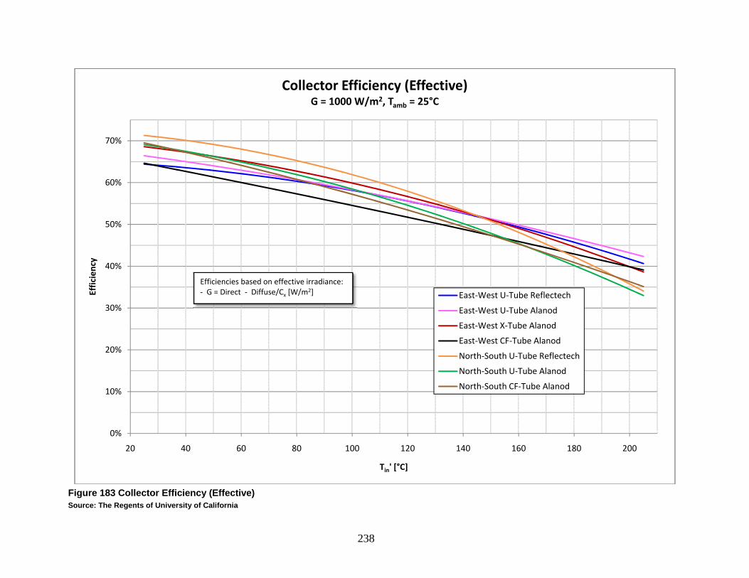
238
Figure 183 Collector Efficiency (Effective) Source: The Regents of University of California
0%
10%
20%
30%
40%
50%
60%
70%
20 40 60 80 100 120 140 160 180 200
Efficiency
Tin' [°C]
Collector Efficiency (Effective)G = 1000 W/m2, Tamb = 25°C
East‐West U‐Tube Reflectech
East‐West U‐Tube Alanod
East‐West X‐Tube Alanod
East‐West CF‐Tube Alanod
North‐South U‐Tube Reflectech
North‐South U‐Tube Alanod
North‐South CF‐Tube Alanod
Efficiencies based on effective irradiance:‐ G = Direct ‐ Diffuse/Cx [W/m2]

239
Figure 184. Collector Efficiency (DNI) Source: The Regents of University of California
0%
10%
20%
30%
40%
50%
60%
70%
80%
90%
20 40 60 80 100 120 140 160 180 200
Efficiency
Tin' [°C]
Collector Efficiency (DNI)GE= 1000 W/m2, Tamb = 25°C
East‐West U‐Tube Reflectech
East‐West U‐Tube Alanod
East‐West X‐Tube Alanod
East‐West CF‐Tube Alanod
North‐South U‐Tube Reflectech
North‐South U‐Tube Alanod
North‐South CF‐Tube Alanod
Efficiencies based on DNI:‐ G = GDirect [W/m2]

240
Possible errors Errors in the data may come from any of the following: instrumental errors, measurement errors, assumed values, tolerance errors, environmental effects, ground reflection, and errors in theory. Although calibrated, instruments such as pyranometers, pyrheliometers, thermocouples and other temperature sensors, the flowmeter, and data acquisition systems may have non‐trivial errors associated with them. While steps were taken to minimize these sources of error, it is impossible to avoid them completely. Errors in any of these instruments would affect the efficiency measurements and/or the temperature scale. The effective area of the collector is a possible source of error due to it being measured manually but this error should be less than a fraction of a percent. Any error in the area of the collector would directly affect the calculated efficiency values. The heat capacity of the oil seems to change over time. Since both of the counterflow and the North‐South U‐Tube with Alanod collectors’ test did not use a calorimeter, the assumed values have an unknown error. An outside source, Rose Consulting, measured the heat capacity of the oil in November 2007 and in September 2009. The measurements in 2007 found the heat capacity of the oil to be less than the table values provided by the oil’s manufacturer while the measurements in 2009 found that the heat capacity was higher than the table values. The September 2009 measurements from Rose Consulting agree well with the heat capacity measured during the East‐West U‐Tube with Alanod tests. The shape of the reflector and the position of the holes in the frame are subject to tolerance errors that would affect the optical efficiency and the acceptance angle. In addition, the surface quality of the reflector surface will affect the results. Soiling of the reflectors and the glass tubes can have a negative effect on the optical efficiency. Ground reflection is inevitable when testing solar thermal collectors outdoors. The amount of ground reflection available to the collector depends on the optics and orientation of the collector, the time of day and the position of the tracker. While the pyranometer mounted on the tracker should be able to detect all or most of the ground reflection, the angle of incidence may be too severe to be accepted by the collector. Collectors with lower concentrations and collectors oriented in a vertical position like the North‐South collectors will be able to accept more of this reflected radiation. The ground reflection will be treated as diffuse light. Ground reflection can cause variation in data and cause East‐West collectors to have an apparent lower than expected performance. Much of the data presented in this report uses an effective irradiance to represent the amount of available power to the collector. The effective irradiance adjustment attempts to take into account that a concentrating optical system cannot accept all of the diffuse and is therefore not considered in the efficiency. Using this method will favor collectors with larger concentration ratios.

241
Other data is presented in this report uses the direct normal irradiance (DNI) to represent the incoming radiation. This method completely ignores diffuse radiation which favors collectors with low concentrations. Using this method with data having a large percent of the irradiance as diffuse can create apparently high efficiencies. Since the testing was done outdoors, it is virtually impossible to test with a constant or consistent ambient temperature. The charts and the data presented in this report attempt to minimize the effect of the differences in the ambient temperature by presenting data with the reduced temperature. Unfortunately, these evacuated tube collectors primarily lose heat through radiation which is non‐linear. In addition, the emissivity of the absorber is a function of the absorber temperature only and not of the ambient temperature. This creates a less than perfect correction for the ambient temperature which is most apparent when a collector was tested during very different outdoor temperatures or when comparing two different collectors that were tested in different seasons. Introduction The history of this public‐private partnership with the XCPC solar thermal project may be instructive to The California Energy Commission as an example how such private‐public partnerships become success stories. When Gary Conley was approached by UC Merced to partner and provide the dominant match, he agreed for H2Go, Inc., his IP development and holding company which spawned SolFocus, the CPV company. However, the SolFocus A‐series had just closed and as he was the co‐founder and CEO, the board asked the thermal grant work be done within SolFocus. Some years later, when the SolFocus “XCPC Concept Loop” had been proved successful, thermal work at SolFocus was acquired back by H2Go to be spun out into B2U Solar, specifically to commercialize the technology. B2U is in the late stages in closing an A‐series round of financing. SolFocus participated in the UC Merced solar thermal project at a rather significant level of cost share because of the promise of cost‐effective heat generation by solar energy. The novel non‐imaging optics technology developed at UC Merced was already well‐know to us from a previous small‐grants Energy Commission project in concentrating photovoltaic. With non‐imaging concentration, fixed solar collectors are capable of generating high temperature in the 200 degree Centigrade range. Moreover, because of the wide angular acceptance (the non‐imaging collectors “see” most of the sky) even diffuse solar radiation is utilized, in contrast to tracking concentrators that “see” only direct insolation. This is particularly important for areas of the world with high diffuse radiation. More importantly, it provides a distinct advantage over solar trough and other concentrator solar thermal designs which turn on or off with each passing cloud, making key applications such as double‐effect chillers difficult if not impossible. The majority of industrial and commercial thermal needs are within the temperature realm provided by this design. As the project developed and we started to see positive results from prototype testing at UC Merced, the company made a significant financial commitment to take the next step and build a

242
“concept loop” of approximately 20 KW Thermal solar energy collectors which would be on the path toward eventual commercialization. Following successful operation of the concept loop at the NASA AMES laboratory in Mountain View California, H2Go decided to take the next critical step on the path to commercialization. A company devoted totally to solar thermal systems and applications, B2U Solar, is being spun out as an independent entity. The solar collector was redesigned with new manufacturing techniques, benefiting from the concept loop experience. In the process, a thorough cost study was performed to indentify the economics of our solar thermal technology as an alternative to natural gas fuel. The company has already delivered product to its first customer, the Gas Technology Institute in Chicago (GTI). GTI will integrate the B2U Solar system to drive the de‐aeration stage of a large industrial boiler in order to demonstrate to the utilities and large corporate customers the viability of the technology. Industrial engineering and pilot production is performed in San Jose and advanced industrial design will be contracted to a major design‐to‐manufacturing firm once funding is completed. Initial series manufacturing is starting in China as our tube manufacturer and early volume customers are also in China. A unique environment exists in China in as they have moved from steam, as used in the US, to oil as the process heat transfer medium, for a number of factors including much higher efficiency and the elimination of high pressure found with steam. Further, the Chinese government is driving renewables through curtailment. That is, a factory owner is capped on the amount of fuel he receives, or the amount of coal he can burn. If he wishes to increase production, an alternative form of fuel must be found. As such, a large appetite for renewable sources has developed. While initial production ramp and installations are made in China, H2Go will install a large variety of demonstrations projections throughout the United States and particularly, in California. These will be conducted in concert with GTI and several major industrial partners, from HVAC to boiler industries. As market development is maturated in the US, production sites will be established throughout the country based upon a range of selection criteria. Finally, an advanced version of the collector was designed and built to be even more efficient and cost effective. We are well on the way to a successful solar thermal business. All these steps are documented in the material to follow. This is with images of actual hardware, real‐life data and economic spread sheets. We believe these developments extend well‐beyond the typical R&D project that is partially funded by state or federal agencies with industry participation. It represents in our view, the emergence of a new, disruptive technology in solar thermal utilization.

243
THE CONCEPT LOOP In 2008, UC Merced and SolFocus requested from The Commission that Tasks 21‐29 be directed toward commercialization efforts with SolFocus as the lead. This was formally approved. SolFocus hired a project manager, Mary Jane Hale with extensive solar experience and a distinguished record at NREL in managing solar thermal programs. SolFocus designed and build a concept thermal loop consisting of 10 North‐South CPC’s modeled after the prototypes at UC Merced, but with a view toward eventual manufacturing and production. The prototype for this concept loop was built at the SolFocus Mt. View, CA facility. Note this was done entirely with SolFocus funds at significant expense. It represents an outstanding commitment of the company which goes well above and beyond typical industry participation in a research project, and is testimony to how seriously the company perceives the promise of high temperature, non‐tracking solar thermal technology. We had the benefit of the UC Merced test loop experience and the UC Merced prototypes which had been fabricated in a furniture factory in Merced. The frame is aluminum and the reflecting material is Alanod, which is a protected silver on aluminum substrate with good solar reflecting properties. Eventually, we expect the Alanod sheet to provide structural stability without need for extensive framing and support. A cost reduction effort using a proprietary reflective structure on different substrates is already underway at H2Go, Inc. The evacuated tube receivers were extruded aluminum with selective coating. The heat transfer characteristics were considered sufficient for the low‐concentration North‐South design. ‐ North‐South: Concentration Factor = 1.15, acceptance angle ~ +/‐ 60 deg An image of the first prototype is shown on the following page.

244
Figure 185. The team leader, Mary Jane Hale is accompanied by members of the SolFocus solar thermal engineering team. Photo Credit: The Regents of University of California
The prototype collector was operated with water at the Mountain View facility. The results were deemed sufficient to proceed to a concept loop of 10 collectors To be deployed at NASA-Ames which is a NASA laboratory situated close to the company in Mountain View. CONCEPT LOOP at NASA AMES Considerable effort was expended in finding a suitable site at NASA AMES with both access and security. We required both electric power for instruments, pumps, etc. as well as a water supply. We decided our initial heat transfer fluid would be water before switching to the DuraTherm 600 heat transfer oil used at UC Merced. The ground had to be prepared and leveled. An enclosure was procured to serve as a command and control center for the concept loop. The concept loop benefited from our experience of the UC Merced test loop, which in our opinion is world-class. No university campus we know of has a thermal collector testing loop with the sophistication and reliability of the UC Merced facility. We are aware of a solar thermal
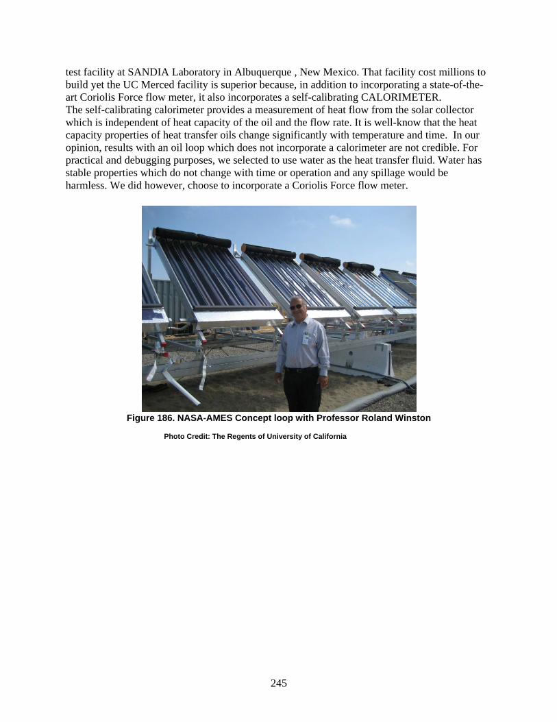
245
test facility at SANDIA Laboratory in Albuquerque , New Mexico. That facility cost millions to build yet the UC Merced facility is superior because, in addition to incorporating a state-of-the- art Coriolis Force flow meter, it also incorporates a self-calibrating CALORIMETER. The self-calibrating calorimeter provides a measurement of heat flow from the solar collector which is independent of heat capacity of the oil and the flow rate. It is well-know that the heat capacity properties of heat transfer oils change significantly with temperature and time. In our opinion, results with an oil loop which does not incorporate a calorimeter are not credible. For practical and debugging purposes, we selected to use water as the heat transfer fluid. Water has stable properties which do not change with time or operation and any spillage would be harmless. We did however, choose to incorporate a Coriolis Force flow meter.
Figure 186. NASA-AMES Concept loop with Professor Roland Winston
Photo Credit: The Regents of University of California

246
Another view of the NASA-AMES Concept loop with project manager Mary Jane Hale and Roland Winston.
Photo Credit: The Regents of University of California
An overall view of the Concept Loop.
Photo Credit: The Regents of University of California
The concept loop with Solar Engineer Francis Truntzer and Roland Winston.
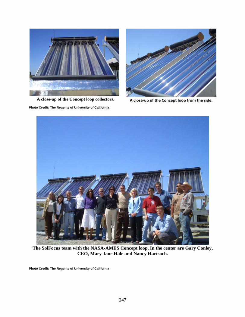
247
A close-up of the Concept loop collectors.
Photo Credit: The Regents of University of California
The SolFocus team with the NASA-AMES Concept loop. In the center are Gary Conley,
CEO, Mary Jane Hale and Nancy Hartsoch. Photo Credit: The Regents of University of California
A close‐up of the Concept loop from the side.

248
TESTING of CONCEPT LOOP The instrumentation for the concept loop was selected for long‐term performance testing in contrast to the instantaneous performance testing done at the UC Merced test loop. Our collectors have fixed orientation, as appropriate to actual use rather than being deployed on tracking stands. The total ground insolation was motored by horizontal EPPLY pyranometers, while a shadow band detector gave information on direct versus diffuse solar radiation. The heat transfer fluid was water, obviating the need for a precision calorimeter such as was used at UC Merced. In some respects we emulated the UC Merced test system. The flow was measure by a Coriolis Force flow meter and the temperatures with thermocouples (not platinum resistance thermometers). There was use of in‐line mixers to ensure the flow stream is well‐mixed before the temperature is measured.
Source: The Regents of University of California
Graph of all day power output performance on December 17, 2008

249
Source: The Regents of University of California *Note that the temperatures in the above graphs correlate to 200°C when using oil. We had to keep the output low to prevent our cooling water from boiling. We employed an evaporative chiller to keep the temperature artificially low.
Graph of temperature achieved
We achieved over 45 kWh of output power over 120° C*

250

251

252

253
The Gas Technology Institute (GTI) Project The first commercial project for B2U Solar is with the Gas Technology Institute in Chicago. GTI ordered an initial 10kWt system composed of 10 B2U NICC panels. These will be integrated with the de-aeration stage of a large industrial boiler to reduce the overall natural gas consumption. The de-aeration stage was selected as it easily accommodated a heat-transfer medium. This stage is where feed water is initially heated to remove dissolved oxygen and where chemicals are added before being fed into the boiler chamber. It consumes up to 20% of the total energy use of an industrial boiler. Following are a series of photographs of the installation: Photo Credit: The Regents of University of California

254
Photo Credit: The Regents of University of California

255
A levelized cost of energy (LCOE) analysis has been developed for several versions of the NICC collector. The results range from ~ 2 cents ‐ ~ 4 cents per kWh depending on collector design, making this an attractive option for displacing natural gas.
B2U Solar LCOE model excerpt - PHX scenario

256
B2U Solar multi-location vs. gas futures Source: The Regents of University of California
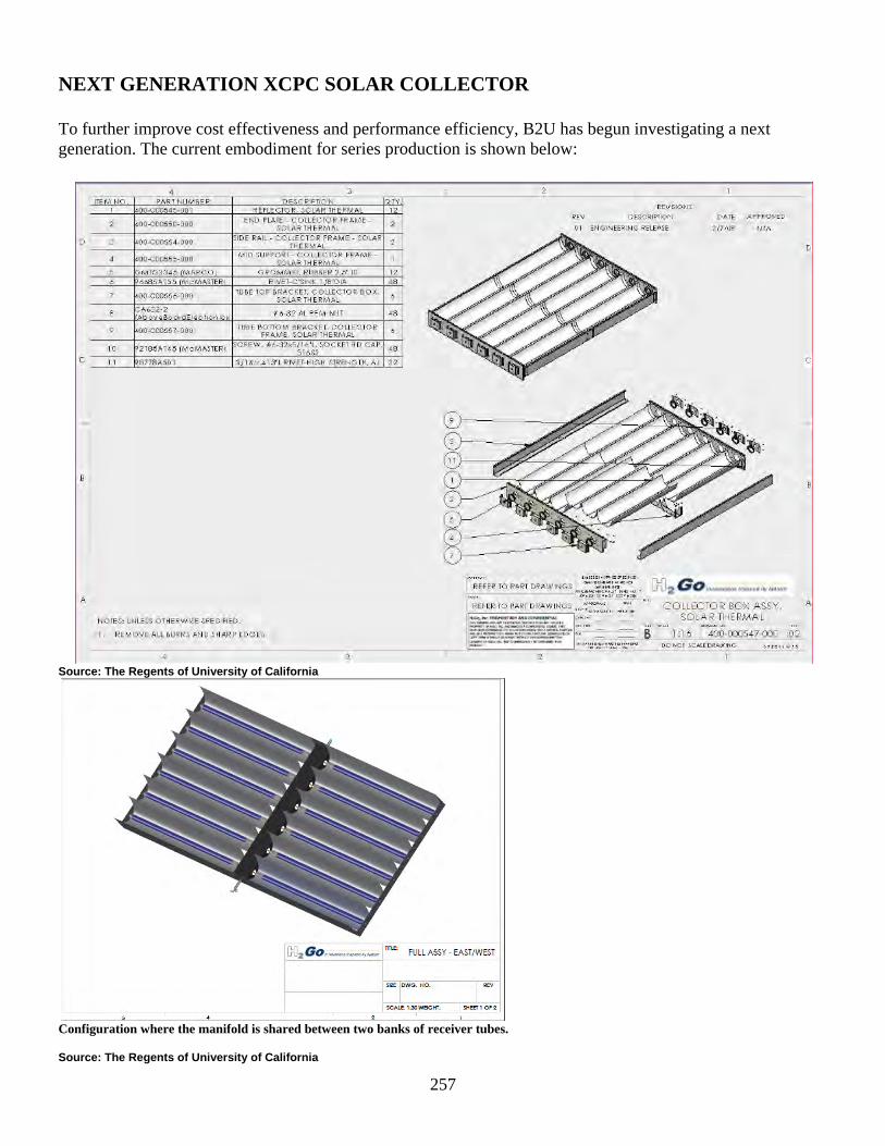
257
NEXT GENERATION XCPC SOLAR COLLECTOR To further improve cost effectiveness and performance efficiency, B2U has begun investigating a next generation. The current embodiment for series production is shown below:
Source: The Regents of University of California
Configuration where the manifold is shared between two banks of receiver tubes.
Source: The Regents of University of California

258
Next generation B2U Solar NICC prototype with shared manifold
Photo Credit: The Regents of University of California
Photo Credit: The Regents of University of California Photo Credit: The Regents of University of California

259
Photo Credit: The Regents of University of California Photo Credit: The Regents of University of California
Front view of next generation XCPC. Notice the spectacular “non‐imaging optics effect” The entire aperture is dark
because all the light is reflected onto the absorber.
Photo Credit: The Regents of University of California Conclusion We have traced the evolution of this California Energy Commission project from proof of concept in a university laboratory (UC Merced) to proof of concept in a quasi industrial setting (NASA‐AMES Concept Loop) to commercialization in a start‐up company (B2U Solar). We believe this is an exemplary success story of progress from public‐private partnership (academia to industry) aided by public support.
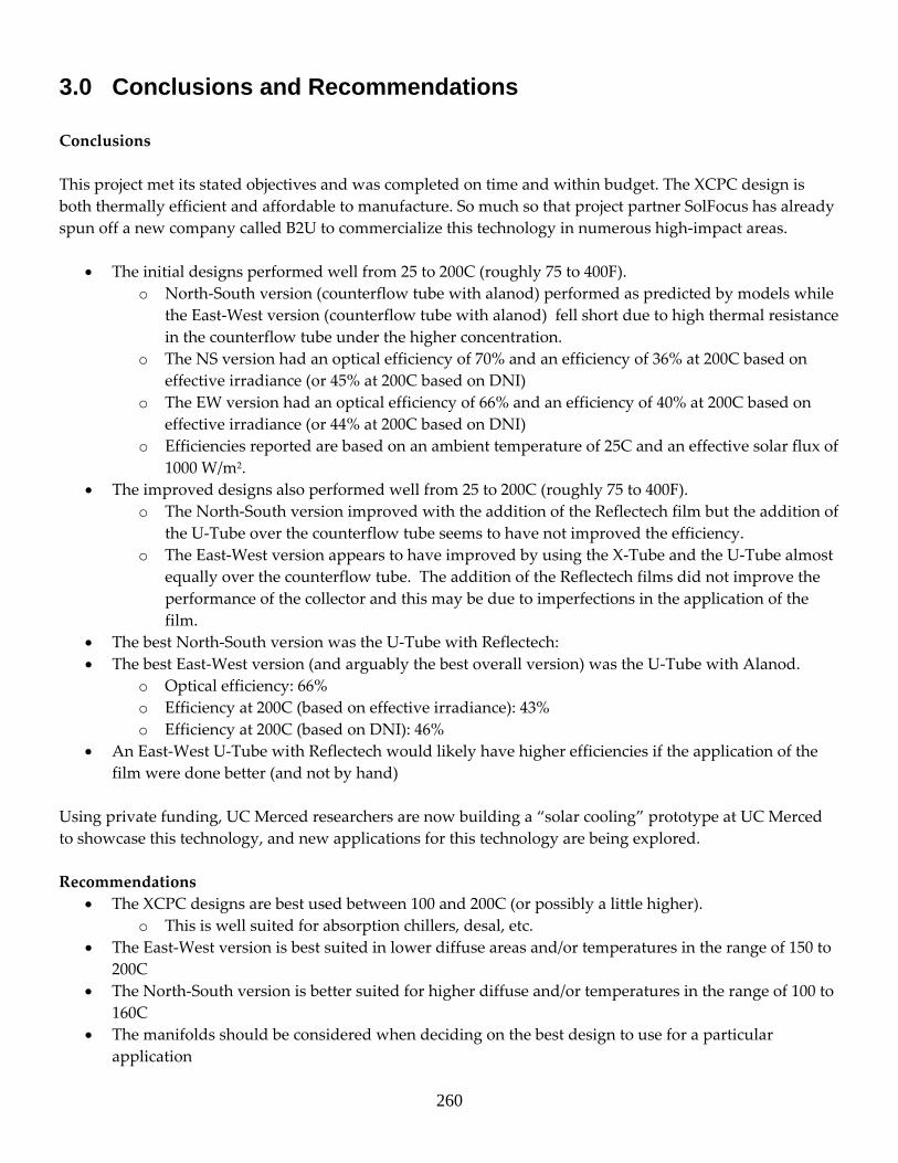
260
3.0 Conclusions and Recommendations Conclusions This project met its stated objectives and was completed on time and within budget. The XCPC design is both thermally efficient and affordable to manufacture. So much so that project partner SolFocus has already spun off a new company called B2U to commercialize this technology in numerous high‐impact areas.
• The initial designs performed well from 25 to 200C (roughly 75 to 400F). o North‐South version (counterflow tube with alanod) performed as predicted by models while
the East‐West version (counterflow tube with alanod) fell short due to high thermal resistance in the counterflow tube under the higher concentration.
o The NS version had an optical efficiency of 70% and an efficiency of 36% at 200C based on effective irradiance (or 45% at 200C based on DNI)
o The EW version had an optical efficiency of 66% and an efficiency of 40% at 200C based on effective irradiance (or 44% at 200C based on DNI)
o Efficiencies reported are based on an ambient temperature of 25C and an effective solar flux of 1000 W/m2.
• The improved designs also performed well from 25 to 200C (roughly 75 to 400F). o The North‐South version improved with the addition of the Reflectech film but the addition of
the U‐Tube over the counterflow tube seems to have not improved the efficiency. o The East‐West version appears to have improved by using the X‐Tube and the U‐Tube almost
equally over the counterflow tube. The addition of the Reflectech films did not improve the performance of the collector and this may be due to imperfections in the application of the film.
• The best North‐South version was the U‐Tube with Reflectech: • The best East‐West version (and arguably the best overall version) was the U‐Tube with Alanod.
o Optical efficiency: 66% o Efficiency at 200C (based on effective irradiance): 43% o Efficiency at 200C (based on DNI): 46%
• An East‐West U‐Tube with Reflectech would likely have higher efficiencies if the application of the film were done better (and not by hand)
Using private funding, UC Merced researchers are now building a “solar cooling” prototype at UC Merced to showcase this technology, and new applications for this technology are being explored. Recommendations
• The XCPC designs are best used between 100 and 200C (or possibly a little higher). o This is well suited for absorption chillers, desal, etc.
• The East‐West version is best suited in lower diffuse areas and/or temperatures in the range of 150 to 200C
• The North‐South version is better suited for higher diffuse and/or temperatures in the range of 100 to 160C
• The manifolds should be considered when deciding on the best design to use for a particular application

261
o North‐South manifolds are easily connected in series due to the fact that they are parallel to the ground.
o East‐West manifolds are more difficult to connect one to another o East‐West manifolds also limit the energy density of the solar field due to spaces between
collectors • Higher R‐Value (per inch) insulation could be used on the manifolds to reduce heat loss. Surface area
of the insulation should be minimized to reduce heat loss. • Higher flowrates will provide a slight increase in efficiency due to lower absorber temperatures but
higher flowrates generally require more power to pump. This trade off should be considered • Both versions could have improved more from the Reflectech film if the application was better.

262
References
http://www.solarpanelsplus.com/images/yazaki‐chiller‐diagram.jpg http://www.eere.energy.gov/de/thermally_activated/tech_basics.html http://www.unity.com.ph/images/faq2.jpg http://www.barber‐nichols.com/images/rankine_cycle.jpg http://www.eere.energy.gov/de/thermally_activated/ http://www.eere.energy.gov/de/thermally_activated/tech_basics.html http://www.adsorptionchiller.bigstep.com/ http://www.energy.ca.gov/pier/iaw/presentations/FIER_LOWE.PDF http://www.malteser‐krankenhaus‐kamenz.de/englisch/install/adschill/adschill.htm Frost and Sullivan Report #7501‐19, 2000 Brasz, J.; Biederman, B. O.; Holdmann, G.; GRC Annual Meeting, 2005 8 http://www.energylan.sandia.gov/sunlab/Snapshot/solartres.htm http://www.xpedio.carrier.com/idc/groups/public/documents/marketing/05‐810‐003‐25.pdf http://www.wastechengineering.com/papers/vacuum_distillation.htm http://www2.hawaii.edu/~nabil/solar.htm http://www.sc.doe.gov/bes/reports/files/SEU_rpt.pdf http://www.utcpower.com/fs/com/bin/fs_com_Page/0,11491,0104,00.html http://www.eere.energy.gov/de/pdfs/absorption_future.pdf Thyrum, Geoffrey, “Critical Aspects of Modeling Heat Pipe Assisted Heat Sinks”, http://www.hhmz.net/news/62/2006‐3‐24_6302344477.html, 2006.