0

Design and Experimentation of a Large ScaleDistributed Stochastic Control Algorithm Applied

to Energy Management Problems

Xavier WarinEDF

France

Stephane VialleSUPELEC & AlGorille INRIA Project Team

France

Abstract

The Stochastic Dynamic Programming method often used to solve some stochastic op-timization problems is only usable in low dimension, being plagued by the curse of dimen-sionality. In this article, we explain how to postpone this limit by using High PerformanceComputing: parallel and distributed algorithms design, optimized implementations and us-age of large scale distributed architectures (PC clusters and Blue Gene/P).

1. Introduction and objectives

Stochastic optimization is used in many industries to take decisions facing some uncertaintiesin the future. The asset to optimize can be a network (railway, telecommunication [Charalam-bous et al. (2005)] ), some exotic financial options of american type [Hull (2008)]. In the energyindustry, a gaz company may want to optimize the use of a gaz storage [Chen and Forsyth(2009)], [Ludkovski and Carmona (2010, to appear)]. An electricity company may want to op-timize the value of a powerplant [Porchet et al. (2009)] facing a price signal and dealing withoperational contraints : ramp contraints, minimum on-off times, maximum number of startup during a period.An integrated energy company may want to maximize an expected revenue coming frommany decisions take :

• which thermal assets to use ?

• how should be managed the hydraulic reservoirs ?

• which customers options to exercice ?

• how should the physical portfolio be hedged with future contracts ?

In the previous example, due to the structure of the energy market with limited liquidity, themanagement of a future position on the market can be seen as the management of a stockof energy available at a given price. So the problem can be seen as an optimization problemwith many stocks to deal with. This example will be taken as a test case for our performancestudies.

In order to solve stochastic optimization problems, some methods have be developed in thecase of convex continuous optimization : The Stochastic Dual Dynamic Programming method[Rotting and Gjelsvik (1992)] is widely used for compagnies having large stocks of waterto manage. When the company portfolio is composed of many stocks of water and manypower plants a decomposition method can be used [Culioli and Cohen (1990)] and the bundlemethod may be used for coordination [Bacaud et al. (2001)]. The uncertainty is usually mod-eled with trees [Heitsch and Romisch (2003)].In realistic modelization of the previous problem, the convexity is not assured. The constraintsmay be non linear as for gaz storage for example where injection and withdrawal capacitiesdepend on the position in the stock (and for thermodynamic reason depends on the past con-trols in accurate model). Most of the time, the problem is not continuous and is in fact a mixedinteger stochastic problem : the commands associated to a stock of water can only take somediscrete values due to the fact that a turbine has only on-off positions, financial positions aretaken for discrete number of stocks... If the constraints and the objectif function are linearized,the stochastic problem can be discretized on the tree and a mixed integer programming solvercan be used. In order to be able to use this kind of modelization a non recombining tree hasto be build. The explosion of the number of leaves of the tree leads to a huge mixed integerproblem to solve.Therefore when the constraints are non linear or when the problem is non convex, the dy-namic programming method developed in 1957 [Bellman (1957)] may be the most attractive.This simple approach faces one flaw: it is an enumerative method and the computationalcost goes up exponentially with the number of state variable to manage. This approach iscurrently used for a number of state variable below 5 or 6. This article introduces the paral-lelization scheme developed to implement the dynamic programming method, details someimprovements required to run large benchmarks on large scale architectures, and presentsthe serial optimizations achieved to efficiently run on each node of a PC cluster and an IBMBlue Gene/P supercomputer. This approach allows us to tackle a simplified problem with 3random factors to face and 7 stocks to manage.

2. Stochastic control optimization and simulation

We give a simplified view of a stochastic control optimization problem. Supposing that theproblem we propose to solve can be set as :

minnct

E

(N

∑t=1

φ(t,ξt,nct)

)(1)

where φ is a cost function depending on time, the state variable ξt (stock and uncertainty,)and depending on the command nct realized at date t. For simplicity, we suppose that thecontrol only acts on the deterministic stocks and that the uncertainties are uncontrolled. Someadditional constraints are added defining at date t the possible commands nct depending onξt.The software used to manage the energy assets are usually separated into two parts. A firstsoftware, an optimization solver is used to calculate the so-called Bellman value until maturityT. The second one will test the Bellman values calculated during the first software run onsome scenarios.

2.1 Optimization partIn our implementation of the Bellman method, we store the Bellman values J at a given timestep t, for a given uncertainty factor occurring at time t and for some stocks levels. These Bell-man values represent the expected gains remaining for the optimal asset management fromthe date t until the date T starting optimization with a given state. Instead of using usual nonrecombining trees, we have chosen to use Monte Carlo scenarios to achieve our optimizationfollowing [Longstaff and Schwartz (2001)] methodology. The uncertainties are here simplifiedso that the model is Markovian. The number of scenarios used during this part is rather small(less than a thousand). This part is by far the most time consuming. The algorithm 1 gives theBellman values J for each time step t calculated by backward recursion. In the algorithm 1,due to the Markovian property of the uncertainty, s∗ = f (s,w) is a realization at date t + ∆t ofan uncertainty whose value is equal to s at date t, where w is a random factor independent ons.

For t := (nbstep− 1)∆t to 0For c ∈ admissible stock levels (nbstate levels)

For s ∈ all uncertainty (nbtrajectory)J̃∗(s, c) = ∞For nc ∈ all possible commands for stocks (nbcommand)

J̃∗(s, c) = min( J̃∗(s, c),φ(nc) + E (J(t + ∆t, s∗, c + nc)|s))J∗(t, :, :) := J̃∗

Figure 1: Bellman algorithm, with a backward computation loop.

In our modelization, uncertainties are driven by brownian motions and conditional expecta-tion in the algorithm 1 are calculated by regression methods as explained in [Longstaff andSchwartz (2001)]. Using Monte Carlo, it could have been possible to use Malliavin methods[Bouchard et al. (2004)], or it could have been possible to use a recombining quantization tree[Bally et al. (2005)].

2.2 Simulation partA second software called a simulator is then used to accurately compute some financial indi-cators (VaR, EEaR, expected gains on some given periods). The optimization part only givesthe Bellman values in each possible state of the system. In the simulation part, the uncertain-ties are accurately described with using many scenarios (many tens of thousand) to accuratelytest the previously calculated Bellman values. Besides, the modelization in the optimizer isoften a simplified one so that calculation are made possible by a reduction in the number ofstate variable. In the simulator it is often much more easier to deal with far more complicatedconstraints so that the modelization is more realistic. In the simulator, all the simulations canbe achieved in parallel, so we could think that this part is embarrassingly parallel as shownby algorithm 2. However, we will see in the sequel that the parallelization scheme used dur-ing the optimization will bring some difficulties during simulations that will lead to someparallelization task to achieve.

3. Distributed algorithm

Our goal was to develop a distributed application efficiently running both on large PC cluster(using Linux and classic NFS) and on IBM Blue Gene supercomputers. To achieve this goal, wehave designed some main mechanisms and sub-algorithms to manage data distribution,load

stock(1:nbtrajectory) = initialStockFor t := 0 to (nbstep− 1)∆t

For s ∈ all uncertainty (nbtrajectory)Gain = - ∞For nc ∈ all possible commands for stocks (nbcommand)

GainA = phi(nc) + E (J∗(t + ∆t, s∗, stock(s) + nc)|s)if GainA > Gain

com = ncGain = GainA

stock(s) += com

Figure 2: Simulation on some scenarios.

balancing, data routage planning, data routage execution, and file accesses. Next sectionsintroduce our parallelization strategy, detail the most important issues and describe our globaldistributed algorithm.

3.1 Parallelization overview of the optimization partAs explained in section 2 we use a backward loop to achieve the optimization part of ourstochastic control application. This backward loop is applied to calculate the Bellman valuesat discrete points belonging to a set of N stocks, which form some N-dimensional cube of data,or data N-cubes.Considering one stock X, its stock levels at tn and tn+1 are linked by the equation:

Xn+1 = Xn + Commandn + Supplyn (2)

Where:

• Xn and Xn+1 are possible levels of the X stock, and belong to intervals of possible values([Xmin

n ; Xmaxn ] and [Xmin

n+1; Xmaxn+1]), function of scenarios and physical constraints.

• The Command is the change of stock level due to the execution of a command on thestock X between tn and tn+1. It belongs to an interval of values: [Cmin

n ;Cmaxn ], function

of scenarios and physical constraints.

• The Supplyn is the change of stock level due to an external supply (in our test casewith hydraulic energy stocks, snow melting and rain represent this supply). Again, itbelongs to an interval of values: [Smin

n ;Smaxn ], function of scenarios and physical con-

straints.

Considering the equation 2, the backward loop algorithm introduced in section 2, a set ofscenarios and physical constraints, and N stocks, the following 6 sub-steps algorithm is runon each computing node at each time step :

1. When finishing the tn+1 computing step and entering tn one (backward loop), minimaland maximal stock levels of all stocks are computed on each computing node, accordingto scenarios and physical constraints on each stock. So, each node easily computes Nminimal and maximal stock levels that defines the minimal and maximal vertexes ofthe N-cube of points where the Bellman values have to be calculated at date tn.

2. Each node runs its splitting algorithm of the tn N-cube to distribute the tn Bellman valuesthat will be to computed at step tn on P = 2dp computing nodes. Each node computes

the entire map of this distribution: the tn data map. See section 3.4 for details about thesplitting algorithm.

3. Using scenarios and physical constraints set for the application, each node computesthe Commands and Supplies to apply to each stock of each tn N-subcube of the tn datamap. Using equation 2 each node computes the tn+1 N-subcube of points where thetn+1 Bellman values are required by each node to process the calculation of the Bellmanvalues at the stocks points belonging to its tn N-subcube. So, each node easily computesthe coordinates of the P′ tn+1 data influence areas or tn shadow regions, and builds theentire tn shadow region map without any communication with others nodes. This solutionhas appeared faster than to compute only local data partition and local shadow regionon each node and to exchange messages on the communication network to gather thecomplete maps on each node.

4. Now each node has the entire tn shadow region map computed at the previous sub-step,and the entire tn+1 data map computed at the previous time step of the backward loop.Some basic computations of N-cube intersections allow each node to compute the P N-subcubes of points associated to the Bellman values to receive from others nodes andfrom itself, and the P N-subcubes of points associated to the Bellman values to sendto other nodes. Some of these N-subcubes can be empty and have a null size, whensome nodes have no N-subcubes of data at time step tn or tn+1. So, each node builds itstn routing plan, still without any communications with other nodes. See section 3.5 fordetails about the computation of this routing plan.

5. Using MPI communication routines, each node executes its tn routing plan and bringsback the Bellman values associated to points belonging to its tn+1 shadow region in itslocal memory. Function of the underlying interconnection network and the machinesize, it can be interesting to overlap all communications, or it can be necessary to spreadthe numerous communications and to achieve several communication sub-steps. Seesection 3.6 for details about the routing plan execution.

6. Using the tn+1 Bellman brought back in its memory, each node can achieve the compu-tation of the optimal commands for all stock points (according to the stochastic controlalgorithm) and calculate its tn Bellman value.

7. Then, each node save on disk the tn Bellman values and some others step results thatwill be used in the simulation part of the application. They are temporary results storedon local disks when exist, or in global storage area, depending of the underlying parallelarchitecture. Finally, each node cancels its tn+1 data map, tn shadow region map and tnrouting plan. Only its tn data map and tn data N-subcube have to remain to process thefollowing time step.

This time step algorithm is repeated in the backward loop up to time step 0. Then some globalresults are saved, and the simulation part of the application is run.

3.2 Parallelization overview of the simulation partIn usual sequential software, simulations is achieved scenario by scenario: the stock levelsand the commands are calculated from date 0 to date T for each scenario sequentially. Thisapproach is obviously easy to parallelize when the Bellman values are shared by each node. Inour case, doing so will mean a lot of time spent in IO. In the algorithm 2, it has been chosen toadvance time step by time step and to do the calculation at each time step for all simulations.

So Bellman temporary files stored in the optimization part are opened and closed only onceby time step to read Bellman values of the next time step.Similarly to the optimization part, at each time step tn the following algorithm is achieved byeach computing node:

1. Each computing node reads some temporary files of optimization results: the tn+1 datamap and the tn+1 data (Bellman values). All these reading operations are achieved inparallel from the P computing nodes.

2. For each trajectory (up to the number of trajectories managed by each node):

(a) Each node simulates the hazard trajectory from time step tn to time step tn+1.

(b) From the current N dimensional stock point SPn, using equation 2, each node com-putes the tn+1 N-subcube of points where the tn+1 Bellman values are required toprocess the calculation of the optimal command at SPn: the tn shadow region coor-dinates of the current trajectory.

(c) All nodes exchange their tn shadow region coordinates using MPI communicationroutines and achieving a all gather communication scheme. So, each node canbuild a complete tn+1 shadow region map in its local memory. In the optimizationpart each node could compute the entire tn+1 shadow region map, but in the simula-tion part inter-node communications are mandatory.

(d) Each node computes its routing plan, computing N-subcubes intersections of tn+1data map and tn+1 shadow region map. We apply again the 2-step algorithm de-scribed on figure 6 and used in the optimization part.

(e) Each node executes its routing plan using MPI communication routines, and andbrings back the Bellman values associated to points belonging to its tn+1 shadowregion in its local memory. Like in the optimization part, depending on the underly-ing interconnection network and the machine size, it can be interesting to overlapall communications, or it can be necessary to spread the numerous communica-tions and to achieve several communication sub-steps (see section 3.6).

(f) Using the tn+1 Bellman value brought back in its memory, each node can computethe optimal command according to algorithm introduced on figure 2.

3. If required by user, data of the current time step are gathered on computing node 0, andwritten on disk (see section 3.7).

Finally, some complete results are computed and saved by node 0, like the global gain com-puted by the entire application.

3.3 Global distributed algorithmFigure 3 summarizes the main three parts of our complete algorithm to compute optimalcommands of a N dimensional optimization problem and to test them in simulation. Thefirst part is the reading of input data files according to the IO strategy introduced in section3.7. The second part is the optimization solver execution, computing some Bellman values in abackward loop (see sections 1 and 3.1). At each step, a N-cube of Bellman values to compute issplit on an hypercube of computing nodes to load balance the computations, a shadow regionis identified and gathered on each node, some multithreaded local computations of optimalcommands are achieved for each point of the N-cube (see section 4.3), and some temporaryresults are stored on disk. Then, the third part tests the previously computed commands.

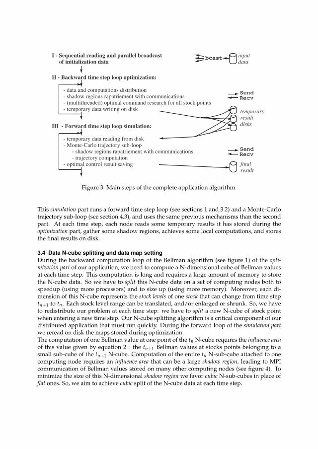
I - Sequential reading and parallel broadcast of initialization data

II - Backward time step loop optimization:

- data and computations distribution - shadow regions rapatriement with communications - (multithreaded) optimal command research for all stock points - temporary data writing on disk

III - Forward time step loop simulation:

- temporary data reading from disk - Monte-Carlo trajectory sub-loop - shadow regions rapatriement with communications - trajectory computation - optimal control result saving

temporary result disks

finalresult

bcastinputdata

Send

Recv

Send

Recv

Figure 3: Main steps of the complete application algorithm.

This simulation part runs a forward time step loop (see sections 1 and 3.2) and a Monte-Carlotrajectory sub-loop (see section 4.3), and uses the same previous mechanisms than the secondpart. At each time step, each node reads some temporary results it has stored during theoptimization part, gather some shadow regions, achieves some local computations, and storesthe final results on disk.

3.4 Data N-cube splitting and data map settingDuring the backward computation loop of the Bellman algorithm (see figure 1) of the opti-mization part of our application, we need to compute a N-dimensional cube of Bellman valuesat each time step. This computation is long and requires a large amount of memory to storethe N-cube data. So we have to split this N-cube data on a set of computing nodes both tospeedup (using more processors) and to size up (using more memory). Moreover, each di-mension of this N-cube represents the stock levels of one stock that can change from time steptn+1 to tn. Each stock level range can be translated, and/or enlarged or shrunk. So, we haveto redistribute our problem at each time step: we have to split a new N-cube of stock pointwhen entering a new time step. Our N-cube splitting algorithm is a critical component of ourdistributed application that must run quickly. During the forward loop of the simulation partwe reread on disk the maps stored during optimization.The computation of one Bellman value at one point of the tn N-cube requires the influence areaof this value given by equation 2 : the tn+1 Bellman values at stocks points belonging to asmall sub-cube of the tn+1 N-cube. Computation of the entire tn N-sub-cube attached to onecomputing node requires an influence area that can be a large shadow region, leading to MPIcommunication of Bellman values stored on many other computing nodes (see figure 4). Tominimize the size of this N-dimensional shadow region we favor cubic N-sub-cubes in place offlat ones. So, we aim to achieve cubic split of the N-cube data at each time step.

n0

n2 n3

n4 n5

n7

Influence area of node 1

Influence area of node 0

n1

Figure 4: Example of cubic split of the N-Cube of data and computations

sub-cubes of results to receive from each node on node 1

sub-cubes of results to send to each node from node 1

n0 n1 n2 n3 n4 n5 n6 n7

n0 n1 n2 n3 n4 n5 n6 n7

Figure 5: Example of routing plan established on node 1

We decided to split our N-cube data on Pmax = 2dmax computing nodes. We successively splitin two equal parts some dimensions of the N-cube, up to obtain 2dmax sub-cubes, or to havereach the limits of the division of the N-cube. Our algorithm includes 3 sub-steps:

1. We split the dimensions of the N-cube in order to obtain sub-cubes with close dimensionsizes. We start to sort the N′ divisible dimensions in decreasing order, and attempt tosplit the first one in 2 equal parts with sizes close to size of the second dimension. Thenwe attempt to split again the size of the 2 first dimensions to reduce their sizes close tothe size of the third one. This splitting operation fails if it leads to a sub-cube dimensionsize smaller than a minimal size, set to avoid to process too small data sub-cubes. Thesplitting operation is repeated up to achieve dmax splits, or up to reduce the sizes ofthe N′ − 1 first dimensions close to the size of the smallest one. Then, if we have notobtained 2dmax sub-cubes we run the second sub-step.

2. Previously we have obtained sub-cubes with N′ close dimension sizes. Now we sortthese N′ divisible dimensions in decreasing order, considering their split dimensionsizes. We attempt to split again in 2 equal parts each divisible dimension in a roundrobin way, up to achieve dmax splits, or up to reach the limit of the minimal size for eachdivisible dimension. Then, if we have not obtained 2dmax sub-cubes we run the thirdsub-step.

3. If it is specified to exceed the minimal size limit, then we split again in 2 equal partseach divisible dimension in a round robin way, up to achieve dmax splits, or up to reachdimension sizes equal to 1. In our application, the minimal size value is set before tosplit a N-cube, and a command line option allows the user to respect or to exceed thislimit. So, when processing small problems on large numbers of computing nodes, some

// Input variable datatypes and declarations on node MeN-cube-coord t DataMaptn+1 [P]N-cube-coord t ShadowRegiontn [P]// Output variable datatypes and declarations on node MeN-cube-coord t LocalRoutingPlanRecv

tn[P]

N-cube-coord t LocalRoutingPlanSendtn

[P]

// Coordinates computation of the N-subcubes to receive on node Me from all nodesFor i := 0 to (P− 1)

LocalRoutingPlanRecvtn

[i] := DataMaptn+1 [i] ∩ ShadowRegionMaptn [Me]

// Coordinates computation of the N-subcubes to send to all nodes from node MeFor i := 0 to (P− 1)

LocalRoutingPlanSendtn

[i] := DataMaptn+1 [Me] ∩ ShadowRegionMaptn [i]

Figure 6: Computation of tn routing plan on computing node Me (0≤ Me < P)

experiments are required and can be rapidly conducted to point out the right tuning ofour splitting algorithm.

Finally, after running our splitting algorithm at time step tn we obtain 2d sub-cubes, and wecan give data and work up to P = 2d computing nodes. When processing small problems onlarge parallel machines, it is possible not all computing nodes will have some computations toachieve at time step tn (P < Pmax) (a too fine grained data distribution would lead to inefficientparallelization). This splitting algorithm is run on each computing node at the beginning oftime step tn. They all compute the same N-cube splitting and deduce the same number ofprovisioned nodes P and the same data map.

3.5 Shadow region map and routing plan computationsDifferent data N-subcubes located on different nodes, or existing at different time steps, canhave shadow regions with different sizes. Moreover, depending on the time step, the problemsize and the number of used computing nodes, the shadow region N-subcube of one computingnode can reach only its direct neighbors or can encompass these nodes. So, the exact routingplan of each node has to be dynamically established at each time step before to retrieve datafrom other nodes.As explained in section 3.1, each node computes the entire shadow region map: a table of Pcoordinates of N-subcubes. In our application these entire maps can be deduced from tn andtn+1 data maps, and from scenarios and physical constraints on commands and supplies ofeach stock. For example, node 1 on figure 4 knows its shadow region (light gray cube) in this3-cube, the shadow region of node 0 (dotted line) and of nodes 2 to 7 (not drawn on figure 4).Then, using both its tn shadow region map and its tn+1 data maps, each computing node caneasily compute its local tn routing plan in two sub-steps:

1. Each node computes the N-subcubes of Bellman values it has to receive from othernodes: the receive part of its local routing plan. The intersection of the tn shadow region N-subcube of node Me with the tn+1 N-subcube of another node gives the tn+1 N-subcubeof Bellman values the node Me has to receive from this node. So, each node achieve thefirst loop of the algorithm described on figure 6, and computes P intersections of N-subcubes coordinates, to get the coordinates of the P N-subcube of Bellman values it

has to receive. When the shadow regions are not too large, many of these P N-subcubesare empty.

2. Each node computes the N-subcubes of Bellman values it has to send to other nodes:the send part of its local routing plan. The intersection of the tn+1 N-subcube of nodeMe with the tn shadow region N-subcube of another node gives the tn+1 N-subcube ofBellman values the node Me has to send to this node. So, each node achieve the secondloop of the algorithm described on figure 6, and computes P intersections of N-subcubescoordinates, to get the coordinates of the P N-subcube of Bellman values it has to send.Again, many of these N-subcubes are empty when the shadow regions are not too large.

Figure 5 shows an example of local routing plan computed on node 1, considering the datadistribution partially illustrated on figure 4. This entire routing plan computation consists in2.P intersections of N-subcube coordinates. Finally, this is a very fast integer computation,run at each time step.

3.6 Routing plan executionNode communications are implemented with non-blocking communications and are over-lapped, in order to use the maximal abilities of the interconnection network. However, forlarge number of nodes we can get small sub-cubes of data on each node, and the influenceareas can reach many nodes (not only direct neighbor nodes). Then, the routing plan exe-cution achieves a huge number of communications, and some node interconnexion networkcould saturate and slow down. So, we have parameterized the routing plan execution withthe number of nodes that a node can attempt to contact simultaneously. This mechanismspreads the execution of the communication plan, and the spreading out is controlled by twoapplication options (specified on the command line): one for the optimization part, and one forthe simulation part.When running our benchmark (see section 5) on our 256 dual-core PC cluster it has been fasternot to spread these communications, but on our 8192 quad-core Blue Gene/P it has been reallyfaster to spread the communications of the simulation part. Each Blue Gene node has to contactonly 128 or 256 other nodes at the same time, to prevent the simulation time to double. Whenrunning larger benchmarks (closer to future real case experiments), the size of the data andof the shadow regions could increase. Moreover, each shadow region could spread on a little bitmore nodes. So, the total size and number of communications could increase, and it seemsnecessary to be able to temporally spread both communications of optimization and simulationparts, on both our PC-cluster and our Blue Gene/P supercomputer.So, we have maintained our communication spreading strategy. When running the applica-tion, an option on the command line allows to limit the number of simultaneous asynchronouscommunications a computing node can start. If a saturation of the communication system ap-pears, it is possible to use it sparingly, spreading the communications.

3.7 File IO constraints and adopted solutionsOur application deals with input data files, temporary output and input files, and final resultfiles. These files can be large, and our main target systems have very different file accessmechanisms. Computing nodes of IBM Blue Gene supercomputers do not have local disks,but an efficient parallel file system and hardware allows all nodes to concurrently access aglobal remote disk storage. At the opposite, nodes of our Linux PC cluster have local disksbut use basic Linux NFS mechanisms to access global remote disks. All nodes of our cluster

can not make their disk accesses at the same time. When increasing the number of used nodes,IO execution times become longer, and finally they freeze.Temporary files are written and read at each time step. However, each temporary result file iswritten during the optimization part by only one node, and is read during the simulation part byonly the same node. These files do not require concurrent accesses and their management iseasy. Depending on their path specified on the command line when running the application,they are stored on local disks (fastest solution on PC cluster), or on a remote global disk (IBMBlue Gene solution). When using a unique global disk it is possible to store some temporaryindex files only once, to reduce the total amount of data stored.Input data files are read only once at the beginning, but have to be read by each computingnode. Final result files are written at each time step of the simulation part and have to storedata from each computing node. In both cases, we have favored the genericity of the file accessmechanism: node 0 opens, accesses and closes files, and sends data to or receives data fromother nodes across the interconnection network (using MPI communication routines). This IOstrategy is an old one and is not always the most efficient, but is highly portable. It has beenimplemented in the first version of our distributed application. A new strategy, relying on aParallel File System and an efficient hardware, will be designed in future versions.

4. Parallel and distributed implementation issues

4.1 N-cube implementationOur implementation includes 3 main kinds of arrays: MPI communication buffers, N-cubedata maps and N-cube data. We have used classic dynamic C arrays to implement the first kind,and the blitz++ generic C++ library [Veldhuizen (2001)] to implement the second and thirdkinds. However, in order to compile the same source code independently of the number ofenergy stocks to process, we have flattened the N-cubes required by our algorithms. AnyN-dimensional array of stock point values becomes a one dimensional array of values.Our implementation includes the following kind of variables:

• A stock level range is a one dimensional array of 2 values, implemented with ablitz::TinyVector of 2 integer values.

• The coordinates of a N-cube of stock points is an array of N stock level ranges, implementedwith a one dimensional blitz::Array of N blitz::TinyVector of 2 integer values.

• A map of N-cube data is implemented with a two dimensional array of P × Nstock level ranges. It is implemented with a two dimensional blitz::Array ofblitz::TinyVector).

• A Bellman value is depending on the stock point considered and on the alea considered.Our N-cube data are arrays of Bellman values function of different aleas in a N-cube ofstock points. A N-cube data is implemented with a two dimensional blitz::Array ofdouble: the first dimension index is the flattened N dimensional coordinate of the stockpoint, and the second dimension index is the alea index.

• Some one dimensional arrays of double are used to store data to send to or to receivefrom another node, and some two dimensional arrays of double are used to store datato send to or to receive from all computing nodes. Communications are implementedwith the MPI library and its C API, that was available on all our testbed architectures.This API requires addresses of contiguous memory areas, to read data to send or tostore received data. So, classic C dynamic arrays appeared a nice solution to implementcommunication buffers with sizes updated at each time step.

Finally, blitz access mechanism to blitz array elements appeared slow. So, inside the com-puting loop we prefer to get the address of the first element to access using a blitz function,and to access the next elements incrementing a pointer like it is possible for a classic C array.

4.2 MPI communicationsOur distributed application consists in loops of local computations and internode communi-cations, and communications have to be achieved before to run the next local computations.So, we do not attempt to overlap computations and communications. However, in a com-munication step each node can exchange messages with many others, so it is important toattempt to overlap all message exchanges and to avoid to serialize these exchanges.When routing the Bellman values of the shadow region the communication schemes can bedifferent on each node and at each time step (see sub-steps 5 of section 3.1 and 2.e of sec-tion 3.2), and data to send is not contiguous in memory. So, we have not used collectivecommunications (easier to use with regular communication schemes), but asynchronous MPIpoint-to-point communication routines. Our communication sub-algorithm is the following:

• compute the size of each message to send or to receive,

• allocate message buffers, for messages to send and to receive,

• make local copy of data to send in the corresponding send buffers,

• start all asynchronous MPI point-to-point receive and send operations,

• wait until all receive operations have completed (synchronization operation),

• store received data in the corresponding application variables (blitz++ arrays),

• wait until all send operations have completed (synchronization operation),

• delete all communication buffers.

As we have chosen to fill explicit communication buffers to store data to exchange, we have usedin place asynchronous communication routines to exchange these buffers (avoiding to re-copydata in other buffers with buffered communications). We have used MPI Irecv, and MPI Isend

or MPI Issend, depending on the architecture and MPI library used. The MPI Isend routinesis usually faster but has a non standard behavior, function of the MPI library and architectureused. The MPI Issend is a little bit longer but has a standardized behavior. On Linux PCclusters where different MPI libraries are installed, we use MPI Issend / MPI Irecv routines.On IBM Blue Gene supercomputer, with an IBM MPI library, we successfully experimentedMPI Isend / MPI Irecv routines.Internode communications required in IO operations to send initial data to each node, or tosave final results on disk in each time step of simulation part (see sub-step 7 of section 3.1), areimplemented with some collective MPI communications: MPI Bcast, MPI Gather.Exchange of local shadow region coordinates in each time step of the simulation part (see sub-step2.c of section 3.2) is implemented with a collective MPI Allgather operation. All these com-munication have very regular schemes and can be efficiently implemented with MPI collectivecommunication routines.

4.3 Nested loops multithreadingIn order to take advantage of multi-core processors we have multithreaded, in order to createonly one MPI process per node and one thread per core in place of one MPI process per core.Depending on the application and the computations achieved, this strategy can be more or lessefficient. We will see in section 5.4 it leads to serious performance increase of our application.

To achieve multithreading we have split some nested loops using OpenMP standard tool orthe Intel Thread Building Block library (TBB). We maintain these two multithreaded imple-mentations to improve the portability of our code. For example, in the past we encounteredsome problems at execution time using OpenMP with ICC compiler, and TBB was not avail-able on Blue Gene supercomputers. Using OpenMP or Intel TBB, we have adopted an in-cremental and pragmatic approach to identify the nested loops to parallelize. First, we havemultithreaded the optimization part of our application (the most time consuming), and secondwe attempted to multithread the simulation part.In the optimization part of our application we have easily multithreaded two nested loops: thefirst prepares data and the second computes the Bellman values (see section 2). However, onlythe second has a significant execution time and leads to an efficient multithreaded paralleliza-tion. A computing loop in the routing plan execution, packing some data to prepare messages,could be parallelized too. But, it would lead to seriously more complex code while this loop isonly 0.15− 0.20% of the execution time on a 256 dual-core PC cluster and on several thousandnodes of a Blue Gene/P. So, we have not multithreaded this loop.In the simulation part each node processes some independent Monte-Carlo trajectories, andparallelization with multithreading has to be achieved while testing the commands in thealgorithm 2. But this application part is not bounded by the amount of computations, but bythe amount of data to get back from other nodes and to store in the node memory, becauseeach MC trajectory follows an unpredictable path and requires a specific shadow region. So, theimpact of multithreading will be limited on the simulation part until we improve this part (seesection 6).

4.4 Serial optimizationsBeyond the parallel aspects the serial optimization is a critical point to tackle the current andcoming processor complexity as well as to exploit the entirely capabilities of the compilers.Three types of serial optimization were carried out to match the processor architecture and tosimplify the language complexity, in order to help the compiler to generate the best binary:

1. Substitution or coupling of the main computing parts including blitz++ classes by stan-dard C operations or basic C functions.

2. Loops unrolling with backward technique to ease SIMD or SSE (Streaming SIMD Ex-tension for x86 processor architecture) instructions generation and optimization by thecompiler while reducing the number of branches.

3. Moving local data allocations outside the parallel multithreaded sections, to minimizememory fragmentation, to reduce C++ constructor/destructor classes overhead and tocontrol data alignment (to optimize memory bandwidth depending on the memoryarchitecture).

Most of the data are stored and computed within blitz++ classes. The blitz++ streamlinesthe overall implementation by providing arrays operations whatever the data type. Overload-ing operator is one of the main inhibitor for the compilers to generate an optimal binary. Toget round this inhibitor the operations including blitz classes were replaced by standard Cpointers and C operations for the most time consuming routines. C pointers and operators ofcode C are very simple to couple with blitz++ arrays, and whatever the processor architec-ture we have got a significant speedup greater than a factor 3 with this technique. See [Vezolleet al. (2009)] for more details about these optimizations.

With the current and future processors it is compulsory to generate vector instructions to reacha good ratio of the serial peak performance. 30− 40% of the total elapsed time of our softwareis spent in while loops including a break test. For a medium case the minimum number ofiterations is around 100. A simple look at the assembler code shows that, whatever the level ofthe compiler optimization, the structure of the loop and the break test do not allow to unrolltechniques and therefore to generate vector instructions. So, we have explicitly loop unrolledthese while-and-break loops, with extra post-computing iterations then unrolling back toget the break point. This method enables vector instructions while reducing the number ofbranches.In the shared memory parallel implementation (with Intel TBB library or OpenMP directives)each thread independently allocates local blitz++ classes (arrays or vectors). The memoryallocations are requested concurrently in the heap zone and can generate memory fragmen-tation as well as potential bank conflicts. In order to reduce the overhead due to memorymanagement between the threads the main local arrays were moved outside the parallel ses-sion and indexed per the thread numbers. This optimization decreases the number of memoryallocations while allowing a better control of the array alignment between the threads. More-over, a singleton C++ class was added to blitz++ library to synchronize the thread memoryconstructors/destructors and therefore minimize memory fragmentation (this feature can bedeactivated depending on the operating system).

5. Experimental performances

5.1 User case introductionWe consider the situation of a power utility that has to satisfy customer load, using the powerplants and one reservoir to manage. The utility equally disposes of a trading entity being ableto take positions on both the spot market and futures market. We do neither consider themarket complete, nor that market-depth is infinite.

5.1.1 Load and price modelThe price model will be a two factor model [Clewlow and Strickland (2000)] driven by twobrownian motions, and we will use a one factor model for load. In this modelization, theprice future F̃(t, T) corresponding to the price of one MWh seen at date t for delivery at dateT evolves around an initial forward curve F̃(T0, T) and the load D(t) corresponding to thedemand at date t randomly evolves around an average load D0(t) depending on time. Thefollowing SDE describes our uncertainty model for the forward curve F̃(t, T) :

dF̃(t, T)F̃(t, T)

= σS(t)e−aS(T−t)dzSt + σL(t)dzL

t , (3)

with zSt and zL

t two brownian motions, σi some volatility parameters.

With the following notations:

V(t1, t2, t3) =∫ t2

t1

σS(u)2e−2aS(t3−u) + σL(u)2 + 2ρσS(u)e−aS(t3−u)σL(u)du,

WS(t0, t) =∫ t

t0

σS(u)e−aS(t−u)dzSu,

WL(t0, t) =∫ t

t0

σL(u)dzLu ,

(4)

the integration of the previous equation gives :

F̃(t, T) = F̃(t0, T)e−

12

V(t0, t, T) + e−aS(T−t)WS(t0, t) + WL(t0, t). (5)

Noting zDt a third brownian motion correlated to zS

t and zLt , σD the volatility, and noting

VD(t1, t2) =∫ t2

t1

σD(u)2e−2aD(t2−u)du,

WD(t0, t) =∫ t

t0

σD(u)e−aD(t−u)dzDu ,

(6)

the load curve follows the following equation:

D(t) = D0(t)e−

12

VD(t0, t) + WD(t0, t). (7)

With this modelization, the spot price is defined as the limit of the future price :

S(t) = limT↓t

F̃(t, T) (8)

The dynamic of a financial product p for a delivery period of one month [tb(p), te(p)] can beapproximated by :

dF(t, p)F(t, p)

= σ̃S(t, p)e−aS(tb(p)−t)dzSt + σL(t)dzL

t , (9)

where :

σ̃S(t, p) = σS(t)

∑ti∈[tb(p),te(p)]

e−aS(ti−tb(p))

∑ti∈[tb(p),te(p)]

1(10)

5.1.2 Test caseWe first introduce some notation for our market products:

P(t) = {p : t < tb(p)} all futures with delivery after t,L(t, p) = {τ : τ < t, p ∈ P(τ)} all time steps τ before t for which the futures product p

is available on the market,P t = {p : t ∈ [tb(p), te(p)]} all products in delivery at t,P = ∪t∈[0,T]P(t) all futures products considered.

Now we can write the problem to be solved:

min E

T

∑t=0

[npal

∑i=1

ci,tui,t − vtSt + ∑p∈P(t)

(te(p)− tb(p))(q(t,p)F(t,p) + |q(t,p)|Bt)]

s.t. Dt =

npal

∑i=1

ui,t − vt + wt + ∑p∈P t

∑s∈L(t,p)

q(s, p)

Rt+1 = Rt + ∆t(−wt + At) (11)

Rmin ≤ Rt ≤ Rmax

qp,min ≤ q(s, p) ≤ qp,max ∀s ∈ [0, T] ∀p ∈ P

yp,min ≤τ

∑s=0

q(s, p) ≤ yp,max ∀τ < tb(p) ∀p ∈ P

vt,min ≤ vt ≤ vt,max

0≤ ui,t ≤ ui,t,max, (12)

where

• Dt is the customer Load at time t in MW

• ui,t is the production of unit i at time t in MW

• vt is spot transactions in MW (counted positive for sales)

• q(t, p) is the power of the futures product p bought at time t in MW

• Bt is the spread bid-ask in euros/MWh taking into account the illiquidity of the market:its double value is the price gap purchase/sale of one MWh

• Rt is the level of the reservoir at time t in MWh

• St = F(t, t) is the spot price in euros/Mwh

• F(t, p) is the futures price of the product p at time t in euros/MWh

• wt is the production of the reservoir at time t in MW

• At are the reservoir inflows in MW

• ∆t the time step in hours

• qp,min, qp,max are bounds on what can be bought and sold per time step on the futuresmarket in MW

• yp,min, yp,max are the bounds on the size of the portfolio for futures product p

• Rmin, Rmax are (natural) bounds on the energy the reservoir can contain.

Some additional values for the initial stocks are also given, and some final values are set forthe reservoir stock remaining at date T.

5.1.3 Numerical dataWe consider at the begin of a month a four months optimization, where the operator can takeposition in the future market twice a month using month ahead futures peak and offpeak, twomonth ahead futures peak and off peak, and three month ahead futures base and peak. So theuser has at date 0 6 future products at disposal. The number of trajectories for optimizationis 400. The depth of the market for the 6 future products is set to 2000 MW for purchase andsales (yp,min = −2000, yp,max = 2000). Every two weeks, the company is allowed to change itsposition in the futures market within the limits of 1000 MW (qp,min = −1000, qp,max = 1000).All the commands for the futures stocks are tested from -1000 MW to 1000 MW with a stepof 1000 MW. The hydraulic command is tested with a step of 1000MW. All the stocks of fu-tures are discretized with a 1000MW step, the hydraulic reservoir is discretized with 225 stepsleading to a maximum of 225 ∗ 56 points to explore for the stock state variables. The maxi-mum number of commands tested is 5 ∗ 36 at day 30 for each point stock. This discretizationis a very accurate one leading to a huge problem to solve. Notice that the number of stocksis decreasing with time. After two months, the two first future delivery periods are past sothe problem becomes a 5 stocks problem. After three months , we are left with a three stocksproblems and no command to test (delivery of the two last future contracts has begun). Theglobal problem is solved with 6 steps per days, defining the reservoir strategy, and the futurecommands are tested every two weeks.

5.2 Testbeds introductionWe used two different parallel machines to test our application and measure its performances: a PC cluster and a supercomputer.

• Our PC cluster was a 256-node cluster of SUPELEC (from CARRI Systems company)with a total of 512 cores. Each node hosts one dual-core processor: INTEL Xeon-3075 at2.66 GHz, with a front side bus at 1333 MHz. The two cores of each processor share 4 GBof RAM, and the interconnection network is a Gigabit Ethernet network built around alarge and fast CISCO 6509 switch.

• Our supercomputer was the IBM Blue Gene/P supercomputer of EDF R&D. It pro-vides up to 8192 nodes and a total of 32768 cores, which communicate through propri-etary high-speed networks. Each node hosts one quad-core PowerPC 450 processor at850 MHz, and the 4 cores share 2 GB of RAM.

5.3 Experimental provisioning of the computing nodesFigure 7 shows the evolution of the number of stock points of our benchmark application, andthe evolution of the number of available nodes that have some work to achieve: the numberof provisioned nodes. The number of stock points defines the problem size. It can evolve ateach time step of the optimization part and the splitting algorithm that distributes the N-cubedata and the associated work has to be run at the beginning of each time step (see section 3.1).This algorithm determines the number of available nodes to use at the current time step. Thenumber of stock points of this benchmark increases up to 3 515 625, and we can see on figure7 the evolution of their distribution on a 256-nodes PC cluster, and on 4096 and 8192 nodesof a Blue Gene supercomputer. Excepted at time step 0 that has only one stock point, it hasbeen possible to use the 256 nodes of our PC cluster at each time step. But it has not beenpossible to achieve this efficiency on the Blue Gene. We succeeded to use up to 8192 nodes ofthis architecture, but sometimes we used only 2048 or 512 nodes.

1E7

1E6

1E5

1E4

1E3

1E2

1E1

1E0 0 20 40 60 80 100 120

num

ber

of s

tock

poi

nts

and

wor

king

nod

es

time steps

nb of stock pointsnb of working nodes on BG with 8192 nodesnb of working nodes on BG with 4096 nodes

nb of working nodes on PC cluster with 256 nodes

Figure 7: Evolution of the number of stock points (problem size) and of the number of workingnodes (useful size of the machine)

However, section 5.4 will introduce the good scalability achieved by the optimization part ofour application, both on our 256-nodes PC cluster and our 8192-nodes Blue Gene. In fact, timesteps with small numbers of stock points are not the most time consuming. They do not makeup a significant part of the execution time, and to use a limited number of nodes to processthese time steps does not limit the performances. But it is critical to be able to use a largenumber of nodes to process time steps with a great amount of stock points. This dynamicload balancing and adaptation of the number of working nodes is achieved by our splittingalgorithm, as illustrated by figure 7.Section 3.4 introduces our splitting strategy, aiming at creating and distribute cubic subcubesand avoiding flat ones. When the backward loop of the optimization part leaves step 61 andenters step 60 the cube of stock points increases a lot (from 140 625 to 3 515 625 stock points)because dimensions two and five enlarge from 1 to 5 stock levels. In both steps the cubeis split in 8192 subcubes, but this division evolves to take advantage of the enlargement ofdimensions two and five. The following equations resume this evolution:

step 61 : 140625 stock points = 225× 1× 5× 5× 1× 5× 5 stock points (13)

step 60 : 3515625 stock points = 225× 5× 5× 5× 5× 5× 5 stock points (14)

step 61 : 8192 subcubes = 128× 1× 4× 4× 1× 2× 2 subcubes (15)

step 60 : 8192 subcubes = 128× 2× 2× 2× 2× 2× 2 subcubes (16)

1E5

1E4

1E3

1E21E41E31E21E1

Exe

cutio

n tim

e (s

)

Number of nodes

PC-cluster, 2processes/nodePC-cluster, 1process+2threads/node

PC-cluster, 1process+2threads/node, SerialOptimsBG/P, 4processes/node

BG/P, 1process+4threads/nodeBG/P, 1process+4threads/node, SerialOptims

Figure 8: Total execution times function of the deployment and optimization mechanisms

subcube sizes =

[min nb o f stock levelsmax nb o f stock levels

]dim1×[ ]

dim2...

step 61 : subcube sizes =

[12

]×[

11

]×[

12

]×[

12

]×[

11

]×[

23

]×[

23

](17)

step 60 : subcube sizes =

[12

]×[

23

]×[

23

]×[

23

]×[

23

]×[

23

]×[

23

](18)

At time step 61, equations 13 and 15 show the dimension one has a stock level range of size 225split in 128 subranges. This leads to subcubes with 1 (min) or 2 (max) stock levels in dimensionone on the different nodes, as summarized by equation 17. Similarly, the dimension two hasa stock level range of size 1 split in 1 subrange of size 1, the dimension three has a stock levelrange of 5 split in 4 subranges of size 1 or 2. . . At time step 60, equations 14 and 16 show therange of dimensions two and five enlarge from 1 to 5 stock levels and their division increasesfrom 1 to 2 subparts, while the division of dimensions three and four decreases from 4 to2 subparts. Finally, equation 18 shows the 8192 subcubes are more cubic: they have similarminimal and maximal sizes in their last six dimensions and only their first dimension canhave a smaller size. This kind of data re-distribution can happen each time the global N-cubeof data evolves, even if the number of provisioned nodes remains unchanged, in order tooptimize the computation load balancing and the communication amount.

5.4 Performances function of deployment and optimization mechanismsFigure 8 shows the different total execution times on the two testbeds introduced in section5.2 for the following parallelizations:

1E5

1E4

1E3

1E21E41E31E21E1

Exe

cutio

n tim

e (s

)

Number of nodes

PC-cluster, T-totalPC-cluster, T-optimPC-cluster, T-simul

BG/P, T-totalBG/P, T-optimBG/P, T-simul

Figure 9: Details of the best execution times of the application

• implementing no serial optimization and using no thread but running several MPI pro-cesses per node (one MPI process per core),

• implementing no serial optimization but using multithreading (one MPI process pernode and one thread per core),

• implementing serial optimizations and multithreading (one MPI process per node andone thread per core).

Without multithreading the execution time decreases slowly on the PC-cluster or reaches anasymptote on the Blue Gene/P. When using multithreading the execution time is smaller anddecreases regularly up to 256 nodes and 512 cores on PC cluster, and up to 8192 nodes and32768 cores on Blue Gene/P. So, the deployment strategy has a large impact on performancesof our application. Performance curves of figure 8 show we have to deploy only one MPIprocess per node and to run threads to efficiently use the different cores of each node. Themultithreading development introduced in section 4.3 has been easy to achieve (parallelizingonly some nested loops), and has reduced the execution time and extended the scalability ofthe application.These results confirm some previous experiments achieved on our PC cluster and on the BlueGene/L of EDF without serial optimizations. Multithreading was not available on the BlueGene/L. Using all cores of each nodes decreased the execution time but did not allowed toreach a good scalability on our Blue Gene/L [(Vialle et al.; 2008)].Serial optimizations introduced in section 4.4 have also an important impact on the perfor-mances. We can see on figure 8 they divide the execution time by a factor 1.63 to 2.14 on thePC cluster of SUPELEC, and by a factor 1.88 to 2.79 on the Blue Gene/P supercomputer ofEDF (depending on the number of used nodes). Moreover, they lead to reach the scalability

limit of our distributed application: the execution time decreases but reaches a new asymptotewhen using 4096 nodes and 16384 cores on our Blue Gene/P. We can not speedup more thisbenchmark application with our current algorithms and implementation.These experiments have allowed to identify the right deployment strategy (running one MPIprocess per node and multithreading) and the right implementation (using all our serial opti-mizations). We analyze our best performances in the next section.

5.5 Detailed best performances of the application and its subpartsFigure 9 shows the details of the best execution times (using multithreading and implement-ing serial optimizations). First, we can observe the optimization part of our application scaleswhile the simulation part does not speedup and limits the global performances and scaling ofthe application. So, our N-cube distribution strategy, our shadow region map and routing plancomputations, and our routing plan executions appear to be efficient and not to penalize thespeedup of the optimization part. But our distribution strategy of Monte carlo trajectories inthe simulation part does not speedup, and limits the performances of the entire application.Second, we observe on figure 9 our distributed and parallel algorithm, serial optimizationsand portable implementation allow to run our complete application on a 7-stocks and 10-state-variables in less than 1h on our PC-cluster with 256 nodes and 512 cores, and in lessthan 30mn on our Blue Gene/P supercomputer used with 4096 nodes and 16384 cores. Theseperformances allow to plan some computations we could not run before.Finally, considering some real and industrial use cases, with bigger data set, the optimizationpart will increase more than the simulation part, and our implementation should scale both onour PC cluster and our Blue Gene/P. Our current distributed and parallel implementation isoperational to process many of our real problems.

6. Conclusion and perspectives

Our parallel algorithm, serial optimizations and portable implementation allow to run ourcomplete application on a 7-stocks and 10-state-variables in less than 1h on our PC-clusterwith 256 nodes and 512 cores, and in less than 30mn on our Blue Gene/P supercomputer usedwith 4096 nodes and 16384 cores. On both testbeds, the interest of multithreading and serialoptimizations have been measured and emphasized. Then, a detailed analysis has shown theoptimization part scales while the simulation part reaches its limits. These current performancespromise high performances for future industrial use cases where the optimization part willincrease (achieving more computations in one time step) and will become a more significantpart of the application.However, for some high dimension problems, the communications during the simulation partcould become predominant. We plan to modify this part by reorganizing trajectories so thattrajectories with similar stocks levels are treated by the same processor. This will allow us toidentify and to bring back the shadow region only once per processor at each time step and todecrease the number of communication needed.Previously our paradigm has been successfully tested too on a smaller case for gaz storage[Makassikis et al. (2008)]. Currently it is used to valuate power plants facing the market pricesand for different problems of asset liability management. In order to make easier the devel-opment of new stochastic control applications, we aim to develop a generic library to rapidlyand efficiently distribute N dimensional cubes of data on large size architectures.

Acknowledgment

Authors thank Pascal Vezolle from IBM Deep Computing Europe for serial optimizations andfine tuning of the code, achieving sensitive speed improvement.This research has been part of the ANR-CICG GCPMF project, and has been supported bothby ANR (French National Research Agency) and by Region Lorraine.

7. References

Bacaud, L., Lemarechal, C., Renaud, A. and Sagastizabal, C. (2001). Bundle methods instochastic optimal power management: A disaggregated approach using precondi-tioner, Computational Optimization and Applications 20(3).

Bally, V., Pags, G. and Printems, J. (2005). A quantization method for pricing and hedgingmulti-dimensional american style options, Mathematical Finance 15(1).

Bellman, R. E. (1957). Dynamic Programming, Princeton University Press, Princeton.Bouchard, B., Ekeland, I. and Touzi, N. (2004). On the malliavin approach to monte carlo

approximation of conditional expectations, Finance and Stochastics 8(1): 45–71.Charalambous, C., Djouadi, S. and Denic, S. Z. (2005). Stochastic power control for wireless

networks via sde’s: Probabilistic qos measures, IEEE Transactions on Information The-ory 51(2): 4396–4401.

Chen, Z. and Forsyth, P. (2009). Implications of a regime switching model on natural gasstorage valuation and optimal operation, Quantitative Finance 10: 159–176.

Clewlow, L. and Strickland, C. (2000). Energy derivatives: Pricing and risk management, Lacima.Culioli, J. C. and Cohen, G. (1990). Decomposition-coordination algorithms in stochastic opti-

mization, SIAM Journal of Control and Optimization 28(6).Heitsch, H. and Romisch, W. (2003). Scenario reduction algorithms in stochastic program-

ming, Computational Optimization and Applications 24.Hull, J. (2008). Options, Futures, and Other Derivatives, 7th Economy Edition, Prentice Hall.Longstaff, F. and Schwartz, E. (2001). Valuing american options by simulation : A simple

least-squares, Review of Financial Studies 14(1).Ludkovski, M. and Carmona, R. (2010, to appear). Gas storage and supply: An optimal switch-

ing approach, Quantitative Finance .Makassikis, C., Vialle, S. and Warin, X. (2008). Large scale distribution of stochastic control

algorithms for financial applications, The First International Workshop on Parallel andDistributed Computing in Finance (PdCoF08), Miami, USA.

Porchet, A., Touzi, N. and Warin, X. (2009). Valuation of a powerplant under productionconstraints and markets incompleteness, Mathematical Methods of Operations research70(1): 47–75.

Rotting, T. A. and Gjelsvik, A. (1992). Stochastic dual dynamic programming for seasonalscheduling in the norwegian power system, Transactions on power system 7(1).

Veldhuizen, T. (2001). Blitz++ User’s Guide, Version 1.2,http://www.oonumerics.org/blitz/manual/blitz.html.

Vezolle, P., Vialle, S. and Warin, X. (2009). Large scale experiment and optimization of a dis-tributed stochastic control algorithm. application to energy management problems,Workshop on Large-Scale Parallel Processing (LSPP 2009), Roma, Italy.

Vialle, S., Warin, X. and Mercier, P. (2008). A N-dimensional stochastic control algorithmfor electricity asset management on PC cluster and Blue Gene supercomputer, 9th

International Workshop on State-of-the-Art in Scientific and Parallel Computing (PARA08),NTNU, Trondheim, Norway.