design and optimization of magnetron sputtering
DESCRIPTION
design and optimization of magnetron sputteringTRANSCRIPT

i
DESIGN, CONSTRUCTION, AND OPTIMIZATION OF A MAGNETRON SPUTTERING
SYSTEM FOR URANIA DEPOSITION
BY
DAVID JOSEPH GENNARDO
THESIS
Submitted in partial fulfillment of the requirements
for the degree of Master of Science in Nuclear Engineering
in the Graduate College of the
University of Illinois at Urbana-Champaign, 2010
Urbana, Illinois
Master‘s Committee:
Professor Brent J. Heuser, Chair
Professor James F. Stubbins

ii
ABSTRACT
A magnetron sputtering system was designed and constructed in accordance with the Nuclear
Energy Research Initiative for Consortia (NERI-C) project on the ―Performance of actinide-
containing fuel matrices under extreme radiation and temperature environments.‖ The system
will initially be used to produce urania (UO2) films with actinide surrogates that will then be
irradiated at high-temperature and used in several fuel characterization studies. Preliminary work
will also use ceria (CeO2) as a surrogate for urania.
A basic reference for magnetron sputtering concepts and film properties is included. The overall
design of the system is then supplied as well as information with regards to component selection.
Particular detail has been provided for the gas distribution system and associated components
because they were the primary responsibility of the author. The work included the procurement
of standard and custom-order components which the author then used in the construction of a
power supply for the operation of solenoid valves and the construction of a gas manifold.
Information containing details pertinent to single crystal growth of urania and ceria including
comparisons with other systems and their respective operating parameters is also provided.
It was also the responsibility of the author to provide quantitative analysis on the behavior of the
Gas Distribution system once it was operational; this represents the second half of the thesis.
Modeling of the gas distribution system was performed which encompassed the predicted
operating range for film growth in the system. An accurate analytical model could not be
determined and the results suggested that this is mostly due to the complex geometry of the
system and flow regime it was operated within. Experimental models can be further developed
once exact operating parameters have been established.
Finally, recommendations for future modeling and construction work are provided. The latter
includes previously selected components prescribed by the final design as well as suggested
future enhancements for increased functionality.
iii
ACKNOWLEDGEMENTS
In case this is the only manuscript I ever produce, first and foremost I have to dedicate this to my
loving parents, Robert and Patricia Gennardo.
I would like to thank my thesis advisor, Professor Brent Heuser, for all the knowledge and
assistance he provided throughout the course of my masters degree. And of course, my thanks to
the rest of the team: Harrison Pappas, Eric Reside, Mohamed Elbakhshwan and Hyunsu Ju.
Furthermore, my sincerest thanks to department head Professor James Stubbins and to Professor
Barclay Jones, as well as Idell Dollison, Becky Meline, Gail Krueger and everyone else in NPRE
for all the academic guidance, personal support and most importantly patience they‘ve shown me
during my many years at U of I. I would not be where I am today if it were not for them.
Finally, I want to take this last opportunity to give a special thanks to Hyunsu and his wonderful
wife Hayoung for their friendship and advice, to my friend Jason Kern and his wife Jessica for
their support, and to Christopher Marks a.k.a. ―the Czar of Cooling‖ for his friendship and
engineering and consulting expertise.

iv
TABLE OF CONTENTS
SECTION…………………………………………………………………...……….………PAGE
1.0 INTRODUCTION .....................................................................................................................1
1.1 Project Background and Objectives .................................................................................1
1.2 Project Mandate ...............................................................................................................3
1.3 Individual Contribution and Scope of Thesis ..................................................................5
2.0 PLASMA SPUTTER DEPOSITION LITERATURE ...............................................................8
2.1 PVD processes and Vacuum Basics ................................................................................8
2.2 Magnetron Sputtering and the Plasma Environment .....................................................10
2.3 Film Morphology and Growth Modes ...........................................................................16
2.4 Other Film Properties Critical to Film Quality ..............................................................18
2.5 Film Growth Factors and Film Properties for Low Temperature Growth .....................22
2.6 A Note on Film Characterization ...................................................................................38
3.0 SYSTEM DESIGN ..................................................................................................................41
3.1 Basis for Design .............................................................................................................41
3.2 Substrate Selection .........................................................................................................55
3.3 Fixturing and Sample Manipulation ..............................................................................58
3.4 Magnetron Sputtering Subsystem ..................................................................................63
3.5 Gas Distribution System ................................................................................................70
3.6 Safety and Support Systems...........................................................................................92
3.7 Maintenance and Cleaning .............................................................................................96
3.8 Sample Storage ..............................................................................................................98
4.0 OPERATING PARAMETERS AND SYSTEM DESIGN COMPARISONS ........................99
4.1 Recommendations for Epitaxial Film Growth ...............................................................99
4.2 Sample Operating Parameters and Configurations for CeO2 Growth .........................101
4.3 Sample Operating Parameters and Configurations for UO2 Growth ...........................105
4.4 Film Growth Rate Optimization ..................................................................................108
4.5 Conclusions ..................................................................................................................113

v
5.0 GAS KINETICS AND METHODOLOGY...........................................................................114
5.1 Gas Dynamics ..............................................................................................................114
5.2 Assumptions Common to All Models..........................................................................142
5.3 A Note on Units ...........................................................................................................143
5.4 Prerequisite and Ancillary Calculations.......................................................................144
5.5 Methodology and Derivations......................................................................................152
6.0 GAS DISTRIBUTION SYSTEM ANALYSIS .....................................................................169
6.1 Experimental Models ...................................................................................................169
6.2 Simple Geometry Model ..............................................................................................176
6.3 Complex Geometry Model ..........................................................................................180
6.4 Flux Correction Models ...............................................................................................184
6.5 Conclusions ..................................................................................................................190
7.0 CONCLUSIONS....................................................................................................................191
8.0 RECOMMENDATIONS FOR FUTURE WORK ................................................................194
8.1 Recommendations for Gas Conductance Modeling ....................................................194
8.2 Recommendations for System Design .........................................................................195
REFERENCES ............................................................................................................................198
APPENDIX A: ADDITIONAL FIGURES AND TABLES .......................................................202
A.1 Additional Photos.........................................................................................................202
A.2 Alternate Plots (Reversed axes) ...................................................................................205
A.3 Supplemental Figures from O‘Hanlon .........................................................................210
APPENDIX B: MATERIALS PROVIDED BY DR. HEUSER .................................................211
B.1 Initiation and Termination Procedures.........................................................................211
B.2 System Schematic ........................................................................................................214
APPENDIX C: COMPUTER CODE PROVIDED BY HYUNSU JU .......................................215
C.1 Cosine Distribution and Correction Output .................................................................215
C.2 Experimental Fit...........................................................................................................217
AUTHOR‘S BIOGRAPHY .........................................................................................................219
1
CHAPTER 1
INTRODUCTION
The research herein presented corresponds to a Nuclear Energy Research Initiative for Consortia
(NERI-C) project on the ―Performance of actinide-containing fuel matrices under extreme
radiation and temperature environments.‖ The project is pertinent to the Advanced Burner
Reactor (ABR) concept for the Advanced Fuel Cycle Initiative (AFCI) Program.
1.1 Project Background and Objectives
The University of Illinois at Urbana-Champaign (UIUC) is the leading member of a consortium
of universities including the University of Michigan, Georgia Institute of Technology, and South
Carolina State University. The consortium will simulate fuels with various levels of actinide
loading and then characterize their performance. The physical processes deemed ―critical to
nuclear fuel performance‖ include thermal conductivity, ―diffusivity, phase separation and
bubble formation‖ [1]. Studies will be conducted on two types of fuels matrices: UO2 and
U-10Zr. These matrices represent the fuel in the current LWR fleet and potential future metal
fuels to be used in an ABR, respectively [1].
The fuel samples will be ―fabricated in thin-film geometry‖ using depleted uranium [1]. Films
will be fabricated with various levels and combinations of actinide surrogates, such as cerium
and neodymium. Stoichiometric films will be produced as well in order to provide a baseline for
comparison. Additionally, single crystal (or epitaxial) films and polycrystalline films will be
fabricated and compared to one another so as to ―permit an evaluation of the effect of grain
boundaries on all of the physical processes‖ being investigated [1].
The films will be ―irradiated with heavy-ion beams‖ at high temperature in order to implant
fission product surrogates, such as molybdenum or xenon, and to ―induce radiation damage‖ in
an environment similar to that found in an operating reactor [1]. The films will then be ―analyzed
with an extensive suite of microanalytical characterization techniques‖ including, but not limited
to, x-ray diffraction (XRD), small angle x-ray scattering (SAXS), Auger electron spectroscopy

2
(AES), Rutherford backscattering spectrometry (RBS), transmission electron spectroscopy
(TEM), time domain thermal reflectivity (TDTR), and secondary ion mass spectrometry (SIMS)
[1]. Research regarding transport and segregation phenomenon will be conducted in terms of
both ―well-controlled ‗single effect‘ experiments‖ and experiments involving ―synergistic
effects‖ which will then be ―directly coupled with molecular dynamics and kinetic Monte Carlo
simulations‖ [1].
According to the project proposal [1], the specific objectives are:
1. Determine dependence of diffusivity and tendency for precipitation of actinide
surrogates in UO2 and U-10Zr with respect to radiation damage (heavy-ion dose),
UO2 stoichiometry, initial actinide surrogate concentration, temperature (up to ~1400
C), and microstructure (extended defect generation and grain boundary area).
2. Determine dependence of diffusivity and tendency for precipitation of implanted
nonvolatile fission products surrogates in UO2 and U-10Zr with respect to radiation
damage (heavy-ion dose), UO2 stoichiometry, initial actinide surrogate concentration,
temperature (up to ~1400 C), and microstructure (extended defect generation and
grain boundary area).
3. Determine dependence of diffusivity and tendency for bubble formation of implanted
fission gases in UO2 and U-10Zr with respect to radiation damage (heavy-ion dose),
UO2 stoichiometry, initial actinide surrogate concentration, temperature (up to ~1400
C), and microstructure (extended defect generation and grain boundary area).
4. Determine the synergistic effect between the actinides and fission products (including
fission gases) on diffusivity, precipitation, and bubble formation.
5. Determine the influence of the microstructure evolution (fission gas bubble
formation, phase separation, lattice defect generation, and grain boundary area) on the
thermal conductivity as a function of temperature.
6. Develop predictive theoretical/computational models that accurately describe the
transport mechanisms at an atomistic level. This will include the effect of vacancy
creation and diffusion on bubble formation and phase separation. The predictive
models will permit extrapolation of fuel performance to environmental conditions not
obtainable in the experimental phase of the proposed work.

3
Accomplishing these objectives will enable a greater ―understanding of fundamental aspects of
radiation damage and fission product incorporation on ABR performance‖ at the microscopic
level and the atomistic level [1]. This knowledge ―is currently lacking in the open literature‖ [1].
1.2 Project Mandate
UIUC and the University of Michigan will be primarily involved in the first five objectives due
to their expertise in materials analysis. The Georgia Institute of Technology is responsible for the
majority of the computational modeling effort. However, it is the sole responsibility of UIUC to
provide film samples to the rest of the consortium members. Initial plans called for the
construction of a new atomic layer by layer molecular beam epitaxy (ALL-MBE) system for
production of uranium films, but cost analysis determined that it was more effective to use an
existing system to produce surrogate films and to construct a new magnetron sputtering system
for uranium-based fabrication.
The Department of Materials Science and Engineering (MatSE) uses an MBE system to fabricate
CeO2 (or ceria) films instead of UO2 (or urania) due to concerns of radioactive contamination in
other research projects conducted with the multi-purpose MBE system. The MBE provides
functionality for epitaxial growth of oxides with the ability to introduce impurities as a
percentage by volume or in the form of monolayers. Lanthanum is used as an actinide surrogate
in the ceria films. A reflection high-energy electron diffraction (RHEED) system allows film
stoichiometry (or chemistry) and growth to be measured in-situ.
It was the responsibility of the Department of Nuclear, Plasma, and Radiological Engineering
(NPRE) to design and construct a magnetron sputtering system for urania deposition. The system
went through two primary design phases. The initial design was for a smaller system when
deliberations for a new MBE system were still underway.
These designs were re-examined and ultimately changed in favor of a more robust magnetron
sputtering system with added functionality so that a new MBE system would no longer be
necessary. This magnetron system is shown in Figure 1.1.

4
Figure 1.1: Primary chamber and Load-lock of magnetron sputtering system
The design of such an intricate system required the participation of several project members over
the course of several months. No one person would have been able to accomplish the design of
such a system in a timely fashion. New team members were added during the construction phase
of the project. Additional members allowed for creative solutions to complex problems. The
actual construction of the system would also have been impossible alone and at times
necessitated multiple people and a crane be involved.

5
Figure 1.2: Project members from left to right: Hyunsu Ju, Eric Reside, Professor Heuser, Harrison
Pappas, Mohamed Elbakhshwan and David Gennardo
1.3 Individual Contribution and Scope of Thesis
During both the design and construction phases of the project, individual responsibilities were
assigned as well as work that required all members contribute. All phases of the project were
overseen and approved by Professor Heuser at set intervals. The responsibilities of the author are
outlined below:
Part of the team responsible for: cost analysis, design, construction and operation of the
custom-built magnetron sputtering system at UIUC;
Designed and built Gas Injection system using standard and custom-ordered components;
Designed and built power supply for operation of solenoid valves;
Aided in selection of turbomolecular and roughing pumps and Baratron pressure gauges;
Aided in construction of main chamber and initial chamber preparation;
Participated in initial chamber operations and sample preparation.

6
Naturally, it will be the focus of this thesis to most thoroughly describe the section of the project
that was the prime responsibility of the author, this being the Gas Injection and Distribution
system. Critical components in its operation, such as the solenoid power supply and gas
manifold, will be detailed accordingly and are pictured at the end of this section in Figures 1.3
and 1.4, respectively. It was also the responsibility of the author to provide quantitative analysis
on the behavior of the Gas Distribution system once it was operational; this represents the second
half of the thesis. Thus the overall structure of the body of the thesis will take the following
form:
1. A basic review of magnetron sputtering concepts and film properties is provided in
Chapter 2 to serve as a basis for understanding the function of the system.
2. An overview of the design is provided in Chapter 3. Component selection will be
elaborated on for each major subsystem or process and focus will be given to those
associated with the Gas Distribution system.
3. Information containing details pertinent to single crystal growth of urania and ceria
including comparisons with other systems and their respective operating parameters is
supplied in Chapter 4.
4. The methodology and modeling for the Gas Distribution system for the predicted
operating range are then discussed in detail in Chapters 5 and 6, respectively.
5. Finally, conclusions and recommendations for future work are presented in Chapters
7 and 8, respectively.
6. Appendix A contains supplemental figures and materials. Appendix B contains
system operations information written and provided by Professor Heuser. Appendix C
contains computer code written and provided by Hyunsu Ju.

7
Figure 1.3: Custom built power supply for operation of system valves
Figure 1.4: Part of the Gas Injection and Distribution system, particularly the solenoid valves with
air lines (center) and the supply air manifold (back far right)

8
CHAPTER 2
PLASMA SPUTTER DEPOSITION LITERATURE
In order to explain the design decisions made while developing the system, a basic understanding
of gas dynamics and sputtering technology is required. The literature surveyed pertains to basic
vacuum technologies and Physical Vapor Deposition (PVD) processes, of which magnetron
sputtering is one. Additional background information is provided relating to the fabrication and
quality of thin films. This information aided in the selection of components and decisions with
regards to design, analysis, and determining an adequate range for operating parameters.
2.1 PVD processes and Vacuum Basics
Physical Vapor Deposition (PVD) processes, also known as thin film processes, ―are atomistic
deposition processes in which material is vaporized from solid or liquid source in the form of
atoms or molecules, transported in the form of a vapor through a vacuum or low pressure
gaseous (or plasma) environment to the substrate where it condenses‖ [2]. There are several
forms of PVD processing, some of the main ones are ion plating, vacuum evaporation, and
sputter deposition. Basics conceptual drawings are pictured below.
Figure 2.1: 1st row (l to r): vacuum evaporation, plasma sputter deposition, plasma sputter
deposition with magnetron, sputter deposition in vacuum. 2nd
row (l to r): ion plating with
evaporation source in plasma environment, ion plating with sputter source, ion plating with arc
vaporization source, Ion Beam Assisted Deposition (IBAD) with evaporation source [2]

9
All of these PVD processes are conducted in a vacuum or ―low pressure gaseous environment‖
[2]. In the most basic sense, a vacuum environment consists of chamber and a pumping system to
evacuate the chamber. For PVD processes, additional component such as a gas injection system
and equipment used to manipulate samples within the chamber are also required. Depending on
the process used, the degree of vacuum required can fall in one of several ranges.
VACUUM RANGES
Degree of Vacuum Pressure Range (Torr)
Low
750 > P > 25
Medium
25 ≥ P ≥ 7.5×10⁻⁴
High
7.5×10⁻⁴ ≥ P ≥ 7.5×10⁻⁷
Very High
7.5×10⁻⁷ ≥ P ≥ 7.5×10⁻¹⁰
Ultrahigh
7.5×10⁻¹⁰ ≥ P ≥ 7.5×10⁻¹³
Extreme ultrahigh 7.5×10⁻¹³ > P Table 2.1: Vacuum Ranges (in Torr) [3]
It should be noted that different texts may use different naming conventions for the degree or
quality of vacuum. For the purposes of film fabrication the system will operate in the medium
vacuum range while achieving an ultimate ―base pressure,‖ or highest attainable pressure
possible, in the very high vacuum range.
There are several reasons why film fabrication is performed at reduced pressure. For instance, a
―low pressure environment provides a long mean free path for collision between the‖ the original
source of the material and the location upon which the particles are deposited [2]. More
importantly, the vacuum environment allows for the control and minimization of contaminants in
a given system.
―A contaminant can be defined as any material in the ambient or on the surface that interferes
with the film formation process, affects the film properties or influences the film stability in an
undesirable way‖ [2]. The effect a contaminant has depends on its location and concentration,
and what type of contaminant it is: gaseous impurity, adsorbed water vapor, debris, etc.
Contamination can be an unknown variable which hinders the reliability or ―reproducibility‖ of
the deposition process.
10
Specific sources of contamination and methods to control or reduce them will be discussed in
Chapter 3 as this was one of the primary considerations throughout the system design. In Chapter
2 contamination will only be mentioned in the context of how it affects film properties or plasma
environment.
2.2 Magnetron Sputtering and the Plasma Environment
The system employs sputter deposition which is often commonly referred to as sputtering.
Sputtering is a process whereby atoms of a solid target are ejected (or vaporized) due to the
―momentum transfer from an atomic-sized energetic bombarding particle‖ impinging on the
target surface [2]. These vaporized particles will then condense upon and coat a substrate
material. Typically sputtering is performed using gaseous ions from a plasma that are then
accelerated and directed toward the target (although it is also possible to use an ion gun in place
of generating ions by producing a plasma). The system uses a plasma produced and controlled by
magnetron guns.
2.2.1 Plasma Environment
―A plasma is a gaseous environment that contains enough ions and electrons to be a good electrical
conductor‖ [2]. Processes that rely on the use of a plasma are referred to as ―plasma processing.‖
For PVD processes plasmas are usually established in ―low pressure gases‖ and are only ―weakly
ionized‖ which means the plasma contains significantly more neutral gas particles than there are
gas ions [2].
Plasmas can serve several different purposes, some simultaneously, depending on the nature of
the PVD process. They can be used as a source of ions or as a source of electrons. This in turn
allows the plasma to perform ―ion scrubbing,‖ which removes adsorbed material from surfaces,
or to activate reactive species by means of dissociation or excitation. Of course it also allows for
the sputtering of material from a target if the plasma ions are directed toward it. Additionally,
plasmas can ―emit ultraviolet radiation which can aid in chemical reaction and surface energetics
by photo-absorption‖ [2]. Finally, the collisions of the particles generated by the plasma with a
surface as well as the ―recombination and de-excitation‖ these species may experience on the
surface can be a good source of thermal energy [2].

11
No matter the desired use of the plasma, plasma uniformity will be an important concern. A more
uniform plasma allows for a more controlled and therefore more reproducible deposition process
environment. Plasma uniformity is primarily dependent on system geometry and the means by
which the plasma was produced. Plasmas can be produced by several means; some are as simple
as charging a DC diode and allowing ―naturally occurring ions‖ to be collected. At higher gas
pressures and higher power levels the electrons will create more ions via increased electron-atom
collisions, eventually forming a visible ―glow discharge‖ [2]. A glow discharge is how most
people recognize an active plasma, it results from there being enough ions present that the light
emitted from de-excitation of the ions between the electrodes is visible. This is the principle
behind fluorescent light bulbs. However, a DC diode generated plasma is not ideal for sputtering
because ―the electrons that are ejected from the cathode are accelerated away from the cathode
and are not efficiently used for sustaining the discharge‖ [2]. A system better suited to
developing thin films uses balanced magnetrons.
2.2.2 Magnetron guns
―Magnetron plasma configurations‖ use magnetic and electric fields ―to confine the electron
path‖ so that it remains close to the surface of the cathode [2]. In this case, the cathode is the
target material to be sputtered and acts as the negative terminal in that it provides an ―electron
emitting‖ surface [2]. Some of the electrons emitted from the cathode are normal to the magnetic
field lines. Due to the Lorentz force, these electrons will then ―spiral around the magnetic field
lines.‖ The gyrofrequency, or ―frequency of the spiraling motion,‖ and gyroradius, or ―the radius
of the spiral,‖ will depend on the exact magnitude and direction of both the electric and magnetic
fields present.
The magnets in the magnetron gun are positioned so that the electrons will follow a ―closed
path‖ and form a ―circulating current‖ on the surface. ―This circulating current may be several
times the current measured in the external electrical circuit‖ [2]. ―This high flux of electrons
creates a high density plasma‖ by means of ―electron-atom collisions and ionization.‖ The
sputter target or cathode will now be ―at a negative potential with respect to the plasma‖ [2].
Some of the positive ions produced in the plasma are extracted and accelerated toward the target
due to the potential difference (or voltage difference). These ions can then ―sputter the target
material‖ thus ―producing a magnetron sputtering configuration‖ [2]. The denser plasma afforded

12
by a magnetron configuration, as compared to the DC diode set-up, allows for more ion
generation and thus a higher sputter rate.
Alternatively, a radio frequency (RF) potential may be applied instead of, or in conjunction with,
a DC potential. ―When an RF potential, with a large peak-to-peak voltage, is capacitively
coupled to an electrode, an alternating positive/negative potential appears on the surface. During
part of each half-cycle, the potential is such that ions are accelerated to the surface with enough
energy to cause sputtering while on alternate half-cycles, electrons reach the surface to prevent
any charge buildup‖ [2]. The prevention of charge build-up on the target can be a useful factor in
film growth and will be discussed in later sections.
Magnetron sputtering configurations can take on several different shapes or sizes. Either
electromagnets or permanent magnets can be used to generate the electromagnetic field
necessary for a magnetron. ―The magnetics can be internal to the target, such as in the planar
magnetron, or can be external to the target‖ [2]. The planar magnetron source is the most simple
and common design and relies on internal magnets. Figure 2.2 is a diagram of an active planar
magnetron sputter configuration.
As mentioned earlier, a nonuniform plasma is considered detrimental. The effects can be seen in
Figure. 2.2 where a groove or ―racetrack pattern‖ has developed on the target because of ―sputter
erosion‖ [2]. This phenomenon occurs because without the addition of external magnets, a planar
magnetron source will be subject to a nonuniform magnetic field along the surface of the target
which will in turn then cause the development of a nonuniform plasma. ―This plasma
nonuniformity‖ results in ―nonuniform bombardment of the cathode surface and nonuniform
sputtering of the cathode material‖ [2]. As an alternative to using additional magnets, a
secondary plasma may be formed with the use of an RF potential and then applied to the target
surface to generate a more evenly distributed plasma overall. Effects on film properties and the
overall system design will be noted later.

13
Fig
ure
2.2
: D
iag
ram
of
an
act
ive
pla
na
r m
ag
net
ron
sp
utt
er s
ou
rce
an
d t
he
acc
om
pan
yin
g p
lasm
a [
4]
No
te:
Th
e el
ectr
on
-orb
it r
ad
ius
ha
s b
een
gre
atl
y e
nla
rged
in
ord
er t
o b
ette
r il
lust
rate
th
e el
ectr
on
tra
jecto
ry [
4]

14
2.2.3 Reactive Sputter Deposition
―The sputtering yield is the ratio of the number of atoms ejected to the number of incident
bombarding particles and depends on the chemical bonding of the target atoms and the energy
transferred by collision‖ [2]. Usually physical sputtering requires a large amount of energy be
transferred from the bombarding particles to the target to ensure sputtering occurs. The minimum
energy required for sputtering or ―sputtering threshold energy‖ is approximately 25 eV which
corresponds to the ―energy needed for atomic displacement‖ in a solid element due to radiation
damage [2]. It should be noted that this value may be considerably higher for compound
materials than a pure element because ―compounds have chemical bonds that are stronger than
those of the elements‖ [2]. In fact, compound targets will almost always exhibit sputtering yields
that are lower than pure elements for this reason. In order to counter this effect, reactive sputter
deposition can be used instead of a compound target.
―Reactive deposition is the formation of a film of a compound either by co-deposition and
reaction of the constituents, or by the reaction of a deposited species with the ambient gaseous or
vapor environment‖ [2]. A film will only form ―if the product of the reacting species is non-
volatile‖ and ―co-deposition of reactive species does not‖ necessarily guarantee a chemical
reaction will occur [2]. Reactive sputter deposition may also occur if the sputtered particles react
with an adsorbed species already on the substrate surface; this includes contaminants.
―Generally, for the low temperature deposition of a compound film, one of the reacting species
should be condensable and the other gaseous‖ [2].
―Reaction with a gaseous ambient is the most common technique.‖ ―The reactive gas may be in
the molecular state‖ (e.g. O2) or in an ―activated state‖ [2]. Activated gases can be either partially
ionized or in an alternative chemical state which reacts more readily (e.g. ozone). As mentioned
earlier, sometimes just being present in the plasma environment near the magnetron will be
enough to activate a reactive species. However, most common reactive gases tend to be of a
lower atomic number and thus are not ideal for energetic bombardment. Typically, a heavier
inert gas, called the ―working gas,‖ is still used to generate the plasma for sputtering and the
lighter reactive gas is present at a lower partial pressure [2]. The partial pressure is defined as the
pressure contributed by each individual gas; the sum of partial pressures yields the total pressure

15
in a system. The partial pressure and overall gas availability of the reactive gas in a sputtering
system can have dramatic affects on film properties and will be discussed later.
Occasionally sputtering rate is not a concern, and it is simply easier to use a compound target.
―In most cases, sputter deposition of a compound material from a compound target results in a
loss of some of the more volatile material.‖ To make up for this loss deposition is performed ―in
an ambient containing a partial pressure of the reactive gas and this process is called ‗quasi-
reactive sputter deposition‘‖ [2]. It follows that the partial pressure of the reactive species needed
will be higher for reactive sputtering with an elemental target than for quasi-reactive sputter
deposition with a compound target.
2.2.4 Steps involved in Film Growth
Now that the basics of the plasma environment and magnetron configuration for reactive sputter
deposition have been provided, the details of process which affect film growth and properties‘
can be elaborated upon.
For this analysis film growth will be considered to proceed in three steps:
1. Transportation of the ―coating species to the substrate‖ [5].
2. Adsorption of said species onto the substrate surface ―or growing coating‖ and ―their
diffusion over this surface, and finally their incorporation into the coating or their
removal from the surface by evaporation or sputtering‖ [5].
3. ―Movement of the coating atoms to their final position within the coating by processes
such as bulk diffusion‖ [5].
A more rigorous development of the process [2] would further delineate the steps involved as
follows:
• Condensation and nucleation of the atoms on the surface;
• Nuclei growth;
• Interface formation;
• Film growth—nucleation and reaction with previously deposited material;
• Post-deposition changes due to post-deposition treatments, exposure to the ambient,
subsequent processing steps, in-storage changes, or in-service changes.

16
The distinctions between nuclei growth and interface formation will not be examined in-depth in
this analysis. Nor will post-deposition changes be discussed in this reference as they are
considered beyond the scope of this thesis and more applicable to future research objectives.
Ultimately, all of these stages are important in the development of the film, but only the first two
stages will be focused on as transportation and condensation will have the greatest affect on film
properties.
2.3 Film Morphology and Growth Modes
Before discussing the film properties in detail, film morphology and growth modes will be
discussed so that later discussion will only refer to applicable conditions. ―The morphology of a
surface is the nature and degree of surface roughness‖ [2]. The morphology of films and the
primary factors that affect film morphology are illustrated in the Structure Zone Model (SZM)
for sputter deposited films. This is also known as the Thornton Model.
2.3.1 Structure Zone Model of Sputter Deposited Materials
Figure 2.3: SZM (or Thornton) model for sputter deposited materials [2]
As shown in Figure 2.3, film morphology can be categorized in one of four growth regimes or
modes. These growth modes are most heavily dependent on the working gas pressure and the
ratio of substrate temperature to the melting temperature of the sputtered material. The
underlying reasons for these primary dependencies vary by growth mode and will be explained
in the next subsection.

17
The four growth modes are named: Zone 1, Zone T, Zone 2, and Zone 3. (Zone T is an
intermediate growth mode found between Zone 1 and Zone 2 that occurs in plasma sputtering
and ion plating.) These molecular dynamics (MD) zones were each ―associated with conditions
where the physics of coating growth was dominated in turn by‖ a particular mechanism [5]. The
mechanisms for the respective zones are: ―1) Atomic shadowing during transport, 2) surface
diffusion, 3) bulk diffusion‖ [5]. Zone T is unique in that is affected by a number of parameters,
the most obvious of which is energetic bombardment.
2.3.2 Zone 1
Zone 1 type film growth occurs at low deposition temperatures and/or high working gas
pressure. Here ―low temperature‖ is defined as T/Tm < 0.3, where Tm is the melting temperature
of the compound being deposited. While the system is being used to produce urania films it will
most likely operate in the Zone 1 and Zone T range because urania has an extremely high
melting temperature. It is important to understand that ―atomistically deposited films generally
exhibit a columnar morphology‖ [2]. This is a ―unique growth morphology that resembles logs
or plates aligned and piled together‖ but they are not ―single crystal grains.‖ This morphology
can be found whether the film is amorphous or crystalline and ―develops due to geometrical
effects‖ [2]. (Materials that have no detectable crystal structure are called amorphous.) Zone 1
structures clearly demonstrate this columnar growth pattern. The structures are ―tapered units
defined by voided growth boundaries‖ or, in other words, there are ―open boundaries between
the columns‖ [5, 2]. Thus the resultant film has a large surface area ―and a film surface with a
‗mossy‘ appearance‖ [2].
2.3.3 Zone T
For the most part Zone T growth occurs in the same temperature and pressure range as that of
Zone 1 growth. In fact, the boundary between Zone 1 and Zone T can ―be envisioned as
resulting from a competition between the effects of energetic particle bombardment which tends
to produce a dense microstructure, and oblique deposition which tends to produce an open
structure‖ [5]. This will be further explained in the appropriate subsections. Zone T growth
structures are also columnar in nature but appear as a more ―fibrous morphology and is
considered to be a transition from Zone 1 to Zone 2‖ [2, 5].

18
2.3.4 Zone 2
Zone 2 structures grow in the ―medium temperature range‖ where 0.3 < T/Tm < 0.5. The ―basic
columnar morphology remains;‖ however, ―metallurgical grain boundaries‖ have begun to form
as actual grains begin to grow. This is due to the increased temperature allowing for further
energy to be available for surface diffusion, a process which requires a minimum activation
energy. The surface diffusion in turn ―allows the densification of the intercolumnar boundaries‖
eliminating voids and thus producing larger grains [5, 2].
2.3.5 Zone 3
―High temperature‖ Zone 3 growth occurs for T/Tm > 0.5. The increased energy available is now
―in accordance with activation energies typical of bulk diffusion.‖ Thus bulk diffusion now
begins to dominate furthering ―grain growth and densification‖ [5]. The grains begin to become
―equiaxed‖ (or relatively equal in size in all dimensions) thus allowing for a more uniform
material. There is also now enough energy for recrystallization which will begin to considerably
alter the originally columnar growth pattern (although there may still be ―single-crystal columns‖
of material present in the film). In effect, the film is being annealed thus relieving many of the
internal stresses in the film that may have been present due to initial lower temperature growth.
In addition to the growth mode, ―the morphology of the depositing film is determined by the surface
roughness and the surface mobility of the depositing atoms with geometrical shadowing and surface
diffusion competing to determine the morphology of the depositing material‖ [2]. (These factors
will be explained in their respective subsections.)
2.4 Other Film Properties Critical to Film Quality
Film morphology is only one of the many film properties of interest. Other relevant film
properties include: stoichiometry, surface coverage, crystallographic orientation, lattice defects
and void formation, film density, and film stress.
2.4.1 Stoichiometry
―Stoichiometry is the numeric ratio of elements in a compound and a stoichiometric compound is
one that has the most stable chemical bonding‖ [2]. The stoichiometry of a deposited compound
can depend on the amount of reactants that are available and/or the reaction probability of the
deposited atoms reacting with the ambient gas before the surface is buried. In reactive sputtering,

19
―injection of the reactive gas is important to insure uniform activation and availability over the
substrate surface‖ [2]. This enables the entire film to have uniform stoichiometry (across the
surface of the substrate).
Initially the system will be used to produce fully stoichiometric compounds, or compounds that
are in their most stable number forms and thus have whole number ratios of constituent parts.
Later in the project timeline, as the films are produced (or later doped) with surrogates, they will
be hypostoichiometric (or substochiometric) in nature. (This means that some of the surrogates
will take the place in atomic (lattice) positions usually occupied by uranium or oxygen.) It is also
possible to produce hyperstoichiometric films (e.g. if there were more oxygen present than in the
normal compound) although these can be more difficult to produce, especially at higher
temperatures (at which the sample may begin to de-oxidize).
2.4.2 Surface Coverage
―Surface coverage is the ability to cover the surface without leaving uncovered areas or
pinholes‖ [2]. Uncovered areas of the surface are commonly called pinholes. ―They can be
formed by geometrical shadowing during deposition‖ (explained later) or are the results of
particulate contaminants on the substrate surface causing the formation of a nodule. Nodules are
a poorly bonded ―local surface feature,‖ that may fall out upon being disturbed (this is called
―pinhole flaking‖). ―Nodules can also originate at any point in the film growth usually from
particulates (―seeds‖) deposited on the surface of the growing film‖ [2]. Pinholes and nodules
would both be considered macroscopic flaws with regards to surface coverage. There is also the
concept of microscopic surface coverage. This idea stems from the surface morphology of the
film and the previously mentioned porosity inherent to films grown in Zone 1 or Zone T of the
Thorton Model. Other factors that affect surface coverage include gas entrapment, energetic
bombardment, the ―angle-of-incidence of the depositing material, nucleation density and the
amount of material deposited‖ [2].

20
2.4.3 Crystallographic Orientation
Another film property which can relate to both the surface coverage and morphology is that of
the crystallographic orientation of the film. ―It is often found that a preferential crystallographic
orientation,‖ sometimes referred to as ―texture,‖ will develop in a deposited films‖ [2]. Texturing
is important because, depending on the orientation of the crystals, it ―can lead to nonisotropic
film properties‖ When growing a film, certain crystallographic planes will be preferred over
others, thus determining the overall orientation of the crystals. However, it is possible to alter the
preferred orientation by adjusting factors such as substrate temperature or the by voltage biasing
[2]. It is even possible to intentionally create an amorphous film of a material that would usually
be crystalline in nature.
2.4.4 Lattice Defects and Voids
Lattice defects can be rudimentarily classified as vacancies (missing atoms), interstitials (too
many atoms in a given lattice position), or dislocations (many types of lattice misalignments).
―During film growth, vacancies are formed by the depositing atoms not filling all of the lattice
positions‖ [2]. Self-interstitials can form when additional compound elements (most likely the
smaller, reactive component) become trapped in the lattice structure in a position not usually
occupied by an atom. (A substitutional interstitial would occur if a foreign particle was located in
the lattice.)
―Voids are internal pores that do not connect to a free surface of the material and thus do not
contribute to the surface area but do affect film properties such as density‖ [2]. Voids can form
due to gas entrapment and release or as a result of vacancy migration and combination (which
may be initiated by atomic shadowing). Lattice defects in the film will affect the electrical
conductivity (or the ―electrical resistivity,‖ as it may be called). Defect and void formation can
also be affected by factors such as substrate temperature and energetic bombardment.
2.4.5 Film Density
Lattice defects and voids can affect a number of other film properties, many of which are simply
associated with film density. Film density, which is also dependent on surface coverage and
morphology, ―is important in determining a number of film properties such as electrical
resistivity, index of refraction, mechanical deformation, corrosion resistance, and chemical etch

21
rate‖ [2]. Geometric effects, such as the angle-of-incidence of the depositing particles, play an
important part in determining the film density for Zone 1 and Zone T growth. Increased substrate
temperature and energetic bombardment can then be used to increase film density or to ―densify
the film.‖ Increasing film density and surface coverage ―is reflected in film properties such as:
better corrosion resistance, lower chemical etch rate, higher hardness, lowered electrical
resistivity of metal films, lowered gaseous and water vapor permeation through the film‖ [2].
2.4.6 Residual Film Stress
―Atomistically deposited films have a residual stress which may be tensile or compressive in
nature‖ [2]. When atoms are quenched (or immobilized) on a surface ―at spacings greater than‖
is normal for the given temperature, a tensile stress is produced in the film. If the situation is
reversed and instead the atoms ―are closer together than they should be,‖ a compressive stress
results [2]. These stresses may be distributed anisotropically in the film and may even lead to a
film subject to tensile stresses in one direction with compressive stresses in another direction [2].
If the stress is too great, a ―tensile stress will relieve itself by micro-cracking the film‖ and a
―compressive stress will relieve itself by buckling‖ the film [2]. (Buckling may cause a ―wavy‖
or ―wrinkled‖ pattern on the film surface.) For normal applications, the film stress should be
minimized. The easiest way to minimize film stress is by producing very thin films. Many of the
films produced will be on the order of hundreds or a few thousand angstroms. This thickness
should be sufficient to avoid the aforementioned deformations.
However, the stress present in the film will still be sufficient to strain the lattice. This lattice
strain ―represents stored energy‖ and in conjunction ―with a high concentration of lattice defects‖
can lower ―the recrystallization temperature in crystalline materials‖ or promote ―room
temperature void growth in films‖ [2]. Yet even these effects can be fully countered with the
careful adjustment of gas pressure and the amount of energetic bombardment ―to find a zero
stress condition.‖ The underlying reasons for why this is possible will be discussed in the gas
pressure and energetic bombardment subsections.

22
2.5 Film Growth Factors and Film Properties for Low Temperature Growth
The factors that affect critical film properties that have been briefly touched upon will now be
discussed in the detail. As stated previously, urania and ceria films grown by the system will be
associated with Zone 1 and Zone T growth modes. These modes are ―dependent on a plethora of
parameters‖ not limited to substrate temperature and working gas pressure. Most notably, these
include: substrate surface characteristics, the system geometry and angle-of-incidence of the
sputtered particles, reactive gas availability, and voltage biasing and energetic bombardment [2,
5]. ―In order to have reproducible film properties each of‖ the following factors will need to ―be
reproducible.‖ [6, 2]
2.5.1 The importance of surface adatom mobility
―Atomistic film growth occurs as a result of the condensation of atoms that are mobile on a
surface,‖ these atoms are referred to as ―adatoms‖ [2]. The most important consideration in
plasma sputter deposition, and in PVD processes in general, is surface adatom mobility.
Invariably, all other growth factors will affect the surface mobility of the adatoms, albeit some of
them will do so indirectly. In turn, the surface mobility will to a large extent dictate the way in
which a film grows and thus impact all film properties.
To clarify, not all atoms ―which impinge‖ upon the substrate surface will become adatoms (or
remain on the surface). Atoms can either be ―reflected immediately, re-evaporate after a
residence time‖ on the surface, or condense and begin to form a film [2]. The ratio of atoms that
condense upon the surface to the total number of impinging atoms ―is called the sticking
coefficient‖ [2]. Furthermore, once a film has been deposited over the initial surface there is also
the possibility for the film itself to be ―re-sputtered‖ (or ejected from the film) effectively
lowering the sticking coefficient.
A sticking coefficient of unity would mean that every particle that makes contact with the
substrate sticks immediately. A sticking coefficient less than unity implies the adatoms have
more energy available to them and thus ―some degree of mobility over the surface before they
condense" or are removed from the surface [2]. ―The mobility of an atom on a surface will
depend on the energy of the atom, atom-surface interactions (chemical bonding), and the

23
temperature of the surface.‖ Similarly, re-evaporation is a function of the same factors as well as
―the flux of mobile adatoms‖ [2].
The reason why certain crystallographic orientations experience preferred growth (as noted
earlier) is because the surface mobility of adatoms varies based on the different ―surface free
energies‖ of different crystal planes. Urania and ceria both have face-centered cubic (FCC)
lattice structures. The (111) plane has a lower surface energy which allows the adatoms to move
more easily for a given energy and thus makes it easier for the adatoms to reach their final
atomic positions in the lattice. This is enables this orientation to grow faster than other possible
orientations. As the energy of the adatoms is increased, this effect becomes proportionally less
important and it is easier to grow other orientations.
Extending this logic, the surface mobility of adatoms has just as noticeable an effect on the
overall surface morphology of the film. Zone 1 growth structures, and columnar growth in
general, is a direct result of low adatom surface mobility. (The low adatom mobility stems
primarily from the gas pressure and low substrate temperature associated with this growth
mode.) ―Computer simulation studies have provided additional support for the proposition that
the columnar zone1/zone T structure is a fundamental consequence of low mobility deposition‖
[5]. Higher mobility is associated with the other growth modes. Finally, high adatom surface
mobility is critical in the production of epitaxial films, particularly at low temperatures [2, 5]. All
of the growth factors that will be elaborated upon in Section 2.5 will be placed in the context of how they
affect adatom surface mobility.
2.5.2 Angle-of-Incidence, System Geometry, and the Substrate Surface
Atoms sputtered ―from a flat, elemental, homogeneous, fine-grained‖ target ―using near-normal
high energy incidence particle bombardment,‖ like that found with magnetron sputtering, are
ejected ―with a cosine distribution‖ [2]. However, ―the mean angle-of-incidence of the depositing
atom flux will depend on the geometry of the system.‖ This is primarily dependent on the
position of the sputter source with regards to the placement of the substrate, but may also depend
on the fixtures by which the substrate is held and whether or not there is anything located
between the substrate and sputter source [2]. Objects in between the sputter source and the

24
substrate will ―shadow‖ the substrate, blocking part or all of the incoming flux of particles from
reaching the substrate (i.e. the substrate is ―in the shadow of the object‖).
Atomic shadowing is when the surface features of the substrate or the growing film shadow other
parts of the surface from the incoming adatom flux. Atomic ―shadowing induces open
boundaries because high points on the growing surface receive more coating flux than valleys,
particularly when a significant oblique component is present in the flux‖ [5, 2]. Additionally,
―substrate surface roughness‖ promotes ―Zone 1 type behavior,‖ or columnar growth, ―by
creating oblique deposition angles‖ [5, 2]. Films that are ―deposited on a smooth surface will
have properties closer to the bulk properties than will‖ films deposited on a rough or uneven
surface [2]. This is because the ―more normal the angle-of-incidence of the depositing atom flux
the higher the density of the film and the more near to bulk values for the materials properties
that can be attained‖ [2]. This also means that if surface roughness causes ―large local variations
in film thickness‖ that the material properties will also vary accordingly. As such, surface
uniformity or ―homogeneity‖ is of great importance.
If the substrate surface is not homogeneous it will also affect the reproducibility of the film
growth. ―The surface chemistry, morphology, and mechanical properties of the near-surface
region of the substrate can be very important to the film formation process‖ and can be altered or
―prepared‖ to ―produce the desired surface properties‖ [2]. Obviously, any contamination on the
surface will affect the film properties. Substrate selection, preparation, and film compatibility
will be discussed further in Chapter 3.
Some of the physical effects due to a non-uniform flux reaching the substrate surface can be
mitigated by using a smaller sample size as well as fixturing enhancements, such as rotation, to
achieve better ―position equivalency‖ along the surface of the substrate. (Position equivalency
means the entire surface will essentially be exposed to the same flux.) This will be discussed
again in Chapter 3.
It has already been noted that when a film grows at low temperature ―the surface roughness
increases because some features or crystallographic planes grow faster than others.‖ The

25
detrimental effects of this have already been explained, but it is possible to compensate for this:
―the surface can be smoothed or ‗planarized‘ by the depositing material or the roughness can be
prevented from developing.‖ These means are typically accomplished with application of voltage
biasing and energetic bombardment and will be discussed in the appropriate subsection. [2]
Finally, growing a film when the sample holder (and therefore the substrate) is positioned off-
axis will affect the film in a similar fashion to increasing surface roughness because it effectively
increases oblique deposition. As a result, ―the columns do not grow normal to the surface but
grow toward the adatom source with a change in column shape‖ [2]. It was also found that
―increasing the tilt angle of the substrates so as to increase the angle-of-incidence of the arriving
deposition flux‖ had the same effect as increasing working gas pressure [5].
2.5.3 Gas Pressure and Thermalization
Sputter deposition is often considered to occur in two regimes with respect to pressure. These
modes are generally referred to as: ―low-pressure plasmas‖ (plasmas with pressure less than 5
mTorr) and ―high pressure plasmas‖ (plasmas with pressure greater than 5 mTorr but typically
less than 50 mTorr) [2]. In ―a low pressure gas environment‖ sputtered particles are transported
from the target to the substrate without gas phase collisions‖ [2]. By extension, the bombarding
―ions reach the target surface with an energy given by the potential drop between the surface and
the point in the electric field that the ion is formed‖ [2]. As a result the sputtered particles will
have a more consistent energy range proportional to energy input into the target surface. At
higher pressures, the ions suffer physical collisions and charge exchange collisions so there is a
spectrum of energies of the ions and neutrals bombarding the target surface‖ [2]. This in turn
leads to a spectrum of energies in the particles sputtered from the target and a less uniform flux.
Furthermore, the ejected particles are also subject to ―gas phase collisions and ‗thermalization‘‖
[2].
Thermalization is a process whereby a high energy particle collides several times with ambient
gas particles as it moves through the gas thus reducing the energy of the initial high energy
particle until it has the same energy as the ambient gas. ―The distance that the energetic molecule
travels and the number of collisions that it must make to become thermalized depends on its
energy, the relative masses of the molecules, gas pressure, and the gas temperature‖ [2].

26
The Ideal Gas model, which will be discussed further in Chapter 5, treats particles as elastically
colliding hard spheres. ―From the Laws of Conservation of Energy and the Conservation of
Momentum the energy, E, transferred by the collision is given by:
2
2cos
)(
4
ti
it
i
t
MM
MM
E
E
where E = energy, M = mass, i = incident particle, t = target particle and θ is the incident angle as
measured from a line joining their centers of masses‖ as shown in Figure 2.4 [2].
Based on this, ―maximum energy transfer occurs when Mi = Mt and the motion is along a path
joining the centers (i.e. θ= 0)‖ [2].
Figure 2.4: Elastic collision between hard spheres [2]
The higher the pressure of the system, the more particles there are available to collide with,
allowing thermalization to occur more readily. Figure 2.5 ―shows the mean free path for
thermalization of energetic molecules in argon as a function of mass and energy‖ [2]. At a
pressure of 5 mTorr (the boundary of the commonly named low and high pressure plasmas) a
heavy particle (like the Uranium used to form UO2) will only travel 8 cm before it is likely
thermalized.

27
Figure 2.5: Distance traveled in Argon gas at various pressures until thermalization occurs for
heavy and light particles with low and high energies [2]
It is important to note that pressure is usually kept below 50 mTorr to prevent gas phase
nucleation before the particles reach the substrate [2]. This effect will be more noticeable at
higher pressures and longer target to substrate distances and will have a detrimental effect on
film quality as it may provide unevenly distributed nucleation sites on the film surface.
Random ―collisional scattering‖ by the inert ―working gas‖ atoms can also increase ―the oblique
component in the deposition flux.‖ [5, 2] Sometimes this is not considered a negative effect and
is used intentionally as ―scattering may be used to advantage to improve the surface coverage by
randomizing the flux direction.‖ On the other hand, ―to produce a more normal incidence pattern,
the sputtered atoms can be collimated‖ [2]. This is shown if Figure 2.6.

28
Figure 2.6: Illustration demonstrating influence of the gas pressure and resulting oblique deposition
flux on the microstructure of the sputtered film [5]
Figure 2.6 shows a shaped substrate being coated by a ring or ―hollow cathode‖ sputter source
using working gas (Argon) pressure of 100 mTorr. Gas scattering and thermalization caused the
substrate to be primarily covered in Zone 1 growth structures. However, a ―Zone T structure
developed on the protected surface because the oblique flux was removed and its formation was
unaffected by the high Argon pressure‖ [5]. It is also important to note that the side wall of the
―trench‖ or recessed area of the substrate experienced poorer film quality (due to an increased
number of voids), as compared to the other Zone 1 structures, because it only received oblique
flux.
Collimating focuses the particles into a beam by blocking particles that are nonparallel to the
collimator (which in this case is most often just a metal baffle). ―Collimation tends to decrease
the tendency of the deposition to produce a columnar morphology in the deposited film‖ by
simultaneously providing a more uniform adatom flux in terms of angle-of-incidence and energy
distribution [2]. (This is because collimation effectively removes adatoms that would have had a
lower surface mobility due to oblique scattering.) Oftentimes it is simply easier to operate the
system at a lower gas pressure than it is to counteract the effects of gas scattering. At low
substrate temperatures, working gas pressure is one of the most important factors in surface
adatom mobility.

29
2.5.4 Reactive Gas Availability
―In reactive deposition, the depositing material must react rapidly or it will be buried by
subsequent depositing material. Therefore, the reaction rate is an important consideration. The
reaction rate is determined by the reactivity of the reactive species, their availability, and the
temperature of the surface‖ [2].
Gas availability is dependent on several factors. Of course this includes the actual amount of gas
being introduced into the system, but it also is dependent on the location of where the gas is
introduced (i.e. system geometry), the getter pumping of the gas (by chemical reactions with the
sputtered material) and the pumping (or evacuation) of the gas out of the main chamber.
Although stated simply, reactive deposition and the associated getter pumping can be a
complicated process:
Reactive gas can react with sputtered metal particles to form the compound material
before it is deposited on the substrate (getter pumping);
Reactive gas can react with metal that had already deposited on the substrate to form the
compound material (getter pumping);
Pure metal can also be buried before reacting with the process gas (thus causing
substoichiometric films or even layers of pure metal) which is a consequence of poor
reactivity or inadequate gas availability;
Compound can form on target and be sputtered off (a certain degree of this may
necessary to ensure compound formation occurs) (this is also getter pumping)
Material may not coat substrate uniformly (partly because of effects previously listed).
The process of reactive deposition and the usage of the reactive gas are illustrated in Figure 2.7.

30
Figure 2.7: Reactive sputter deposition and the reactive gas supply
Note: Substrate and sputter target positions are inverted as compared to set-up of this system.
Reduced gas availability can be compensated for by increasing the ―reactivity‖ of the gas species
or by using an alternate reactive gas. As previously mentioned, oftentimes the plasma
environment itself will activate the species by means of:
•Dissociation of the species into more chemically reactive radicals (e.g. O2 + e-2O
o) [2];
•Production of new species which may be more easily absorbed and/or are more chemically
reactive (e.g. Oo + O2 O3) [2];
•Ion production;
•Production of short wavelength photons (UV-rays) that can ―stimulate chemical reactions or
create metastable excited states‖ [2];
•―Generating energetic electrons that stimulate chemical reactions‖ [2];
•Energetic ―bombardment enhanced chemical reactions‖ [2].
The means by which the gas is introduced may also increase the reactivity. If a reactive gas, such
as O2, is mixed with an inert gas, such as Argon, before it is introduced into the system it may
undergo ―Penning excitation.‖ Penning excitation is the excitation of an atom ―by the transfer of
the excitation energy from a metastable atom whose excitation energy is greater than‖ the
excitation energy of the first atom‖ [2]. Argon is known to have two metastable states that may
develop when used to create a plasma. Similar to Penning excitation, ―Penning ionization‖ is also
known to occur in ―‗mixed plasmas‘ containing more than one species‖ even if one of the species
is only present in trace quantities [2]. This may cause the ionization of the reactive species.

31
In addition to the effects on stoichiometry, ―reactive gases in the deposition system can influence
the growth, structure, morphology and properties of the deposited films‖ by reducing the adatom
surface mobility [2, 5]. In particular, ―active species such as oxygen have been found to‖
―promote zone 1 structures.‖ Accordingly, ―Zone 1 structures are commonly encountered in
reactive sputtering at low T/Tm in the absence of ion bombardment‖ [5].
In a similar manner, gaseous impurities may also dramatically impact film microstructure even
though present at significantly lower partial pressures because ―residual gas absorption can cause
mobility variations over exposed crystallite surfaces‖ which may lead to a nonuniform film [5].
If the residual gas partial pressure is high (comparatively speaking), it will have ―a major effect
on the surface mobility and the development of columnar morphologies,‖ even for ―high
deposition temperatures‖ [5, 2]. However, it is critical to note that the gas ―scattering effect has a
much greater influence on the coating structure than the‖ reduction in adatom mobility
―associated with absorbed inert gas species on the substrate surface‖ or due to interactions with
the reactive species [5, 2].
2.5.5 Substrate Temperature and other considerations
As previously noted, ―substrate temperature is probably the single most important parameter in
thin film growth.‖ ―At sufficiently high temperatures bulk chemistry and diffusion dominate, so
that a coating loses all memory of the earlier steps in its growth‖ [5]. Increased substrate
temperature will increase surface adatom mobility and can increase reactions involved in
formation of the desired film compound. A high substrate temperature can also prevent other
deleterious effects such as gas entrapment.
―Bombardment of the growing film by a gaseous species can result in the gas being incorporated
into the bulk film since the surface is being continually buried under new film material‖ [2]. A
heated substrate will ―desorb the gases before they are covered over‖ and will prevent this ―gas
incorporation.‖ A substrate temperature of 400°C should be sufficient to prevent incorporation of
Argon into the growing film [2]. Alternatively, maintaining constant bombardment energy (less
than 250 eV) ―will prevent the physical penetration of‖ argon ions into the film without inducing
damage to the film [2].

32
2.5.6 Voltage Biasing and Energetic Bombardment
The final growth factor to be discussed is that of energetic bombardment. It acts in concert with
many of the other factors, although it is not an underlying mechanism like surface adatom
mobility. Concurrent energetic bombardment of the growing film is one of the most important
but often over-looked parameters in magnetron sputtering [2]. Part of the reason for this neglect
may come from the fact that the amount of bombardment and the energy transferred are
complicated processes that cannot be directly controlled by any one operating parameter. Having
an additional means of control for energetic bombardment can allow for greater reproducibility
in film fabrication. Voltage biasing is commonly used as a means of inducing and controlling
energetic bombardment.
Voltage biasing is the application of a negative or positive voltage to the substrate and/or the
sample holder to which it is attached. (Voltage biasing can also be used to solely prevent or
reduce bombardment, although this is a less common use.) To prevent any confusion, sputtering
with a voltage bias applied to the substrate may technically be considered ion plating,
particularly if the reactive gas or sputter material is intentionally ionized. For the purposes of this
work, it will still simply be referred to as plasma sputtering but it will be noted that the film is
subject to energetic bombardment and/or a bias.
Energetic bombardment is an overarching term applied to all particles that impact the growing
film that are not adatoms used to produce the desired compound. ―In addition to bombardment
by‖ the inert and reactive gas ions produced in the plasma, or from ―an independent ion source,
the surface of a growing coating during sputter deposition may be bombarded by sputtered atoms
having energies in the 10-40 eV range, and energetic neutral working gas atoms (ions that are
neutralized and reflected at the sputtering target) having energies as high as several hundred eV‖
[5].
―Reflected neutrals are particularly important‖ in imparting energy to a concurrently bombarded
film but are not affected by voltage biasing [5]. A negative voltage bias would attract the (inert)
working gas ions and repel reactive gas ions. (Naturally, it would also repel electrons that may
escape the magnetic field of the magnetron and head toward the substrate though the effects of

33
these electrons are considered insignificant compared to the energy imparted by entire atoms or
molecules.) If a sputter target atom becomes ionized as it travels through the plasma and were to
impact upon the substrate it is called ―film ion bombardment‖ because the ion is one of the
constituent elements in the film. (It would then most likely react with the reactive gas on the
surface of the film if there is enough availability.) Positive films ions produced by sputtered
metal would be attracted to a negatively voltage biased substrate. This effect can be used to
intentionally produce a more normal angle of incidence to increase film quality.
The applied target voltage, working gas pressure, and working gas to target mass ratio are also
important and adjustable parameters pertaining to energetic bombardment; however, they may be
inconvenient to change (e.g. an alternate working gas) or may negatively affect other parameters
(e.g. gas pressure) while only minimally increasing the effect of bombardment. The growth
factors, which have been discussed previously, affect the bombarding flux in the same fashion as
they affected the incoming adatom flux. ―The energy flux carried to the substrate by the
neutralized and reflected ions‖ will be greater and more uniform at low pressures (< 5 mTorr)
where thermalization does not occur [2]. Again, a more normal incidence will produce a denser
and more uniform film. Finally, a heavier working gas will impart more energy to the sputtered
target atoms and impart more energy themselves when colliding with the substrate, both of
which will increase the energy transferred to the growing film.
―The amount of bombardment is often measured by the amount of depositing material that is
sputtered from the growing film or the addition energy per depositing atom that is added to the
surface‖ [2]. As noted earlier, high energy bombardment effectively reduces the sticking
coefficient (i.e. it causes resputtering of the depositing material), the apparent decrease in the
coefficient (or the sputtering yield) can be used to gauge the amount of bombardment.
The actual effects of bombardment are numerous. Bombarding particles can merely reflect off
the surface without much energy transfer (perhaps due to a glancing collision with the surface or
due to low initial energy) or higher energy ―bombarding particles can physically penetrate into
the surface region.‖ The ―collision effects‖ from these particles will extend back to the near-
surface region. The high energy bombarding ―particle creates a collision cascade and some of the

34
momentum is transferred to surface atoms, hence the possibility of re-sputtering, but more than
95% of the transferred energy ―appears as heat in the surface region and near surface region‖ [2].
―This heating can allow atomic motion such as diffusion and stress annealing, during the film
formation process‖ just as would occur from increasing the substrate temperature through more
conventional means. ―If the thermal conductivity of the film is low the surface region of the film
can have an increasingly higher temperature as the film grows in thickness.‖ If this heating is
applied for a long enough time and the film is of significant thickness, ―the temperature of the
bulk of the material can be kept very low‖ as compared to the surface, enabling ―the
development of a very high temperature gradient in the surface and near surface regions.‖ If
carefully controlled (so as not to exceed the maximum temperature of the sample holder and
stage), this technique may be used to better simulate nuclear fuel conditions which experience
extremely large gradients due to fission. [2]
Additionally, particle bombardment of the growing film ―causes ‗atomic peening‘ where surface
atoms are struck and recoil into voids and interstitial sites in the lattice of the surface region‖ [2].
This process causes the densification of the material and may produce compressive stresses in
the film depending on the amount of bombardment. Yet the disadvantages afforded by increased
stress are more than offset by the ability to correct for lattice defects, such as vacancies. The
knock-on atoms (or atoms displaced from their initial lattice position by collision with the
incident bombarding particle) ―of the coating material are driven into the bulk where they tend to
fill the microvoids that appear to be an inherent consequence of low T/Tm deposition‖ [5].
The number of lattice defects decreases as the bombarding energy increases until it reaches a
value that is approximately 200 eV, at which point the net amount of lattice defects increase once
more. Too much bombardment (at too high an energy) can damage the lattice structure until
eventually the film is amorphized (or becomes amorphous).
Larger surface defects can also be removed or ―smoothed‖ by the re-sputtering and subsequent
re-deposition of the film to remove surface peaks and fill in valleys or ―vias.‖ This process is
called ―planarization‖ and can be important in the production of epitaxial films.

35
As is the case for any sputter grown film, ―the surface and near-surface region is continually
being buried,‖ thus the bombardment effects are trapped in the growing film. This can lead to the
―trapping of the bombarding species at lattice defects‖ or to inert gas entrapment [2]. However if
the deposition rate is low and the bombardment is carefully controlled, the opposite is true.
Energetic bombardment, and the re-sputtering it causes, can cause removal of contaminants from
the growing film. (This includes entrapped working gas or any other residual gases that may
have adsorbed to the surface of the substrate or growing film.)
Additional bombardment effects include ―production of secondary electrons that are accelerated
away from the cathode/substrate surface‖ and ―enhanced chemical reactivity‖ on the film surface
(also known as ―bombardment-enhanced chemical-reactivity‖).
―It is well established that intense energetic ion bombardment during deposition can largely
suppress the development of open zone 1 structures at low T/Tm. This has been demonstrated for
both conducting and nonconducting deposits‖ [5]. (Therefore voltage biasing is applicable to
compounds such as urania and ceria.) This is the reason the transition pressure between Zone 1
and Zone T increases ―with the cathode operating voltage and the target-to-working gas mass
ratio‖ because these parameters correspond to an increase in the ―energy flux carried to the
substrate by the reflected neutrals‖ which in turn suppresses Zone 1 growth structures [5]. The
―increased surface mobility, increased nucleation density and erosion/re-deposition of the
depositing adatoms‖ due to energetic bombardment disrupts the columnar microstructure and
eliminates ―porosity along the columns.‖ This increases film density, ―improves surface
coverage and decreases the pinhole porosity‖ (or macroscopic porosity) of the film [5].
When bombardment is used in addition to gas scattering, which can create an entirely random
flux of adatoms distributed across the substrate surface given the right geometry and pressure,
the surface covering ability can be increased further. These two effects applied in conjunction
also have the added benefit of ―balancing‖ each other. The tensile stress caused by gas scattering
(and the resultant Zone 1 growth structures) and the compressive stress from bombardment (and
resultant Zone T growth structures) may cancel and the deposited film will have a lower stress

36
overall. Similarly, lowered adatom mobility from thermalization may be countered by the energy
flux from the bombardment increasing mobility.
Figure 2.8 shows a comparison between to two sputter deposited films where all parameters are
held constant except for voltage biasing. Film A (left) was not subject to a bias and consequently
had no appreciable bombardment during deposition. A 500 volt bias was applied to Film B
(right). The top two pictures compare the surface morphologies. The bottom two pictures
compare ―fracture cross sections.‖ The difference in film quality can be easily distinguished with
only a preliminary visual examination. ―Film B was denisified‖ as a result of the bombardment
and had a much smoother surface and did not possess porous columnar structure‖ [2]. Although
this is a picture of a metal film, the results will still be similar to those witnessed in reactive
deposition. (A compound film may experience a slight decrease in quality and have more
columnar structures due to the decreased adatom mobility caused by the reactive gas, or this
effect may be offset by the increase in chemical reactivity due to bombardment. The exact results
will depend heavily on pressure, availability, and the particular species reacting.)
Specific voltage bias settings (and other operating parameters) and their application to urania and
ceria films fabricated in the magnetron sputtering system will be mentioned further in Chapter 4.

37
Figure 2.8: Surface (top) and cross-section (bottom) images of a Chromium film grown (a) with no
bias and (b) with a negative 500 V bias (which caused bombardment)
Now that the film properties measured to gauge the quality of film and the numerous growth
factors that affect them have been addressed, the final subsection will briefly describe how these
qualities are measured and the film is characterized. The techniques described therein will be
used to describe the film and examine properties associated with ―film quality.‖
38
2.6 A Note on Film Characterization
Several different techniques will be used to analyze or characterize the film samples fabricated in
the magnetron sputtering system. It has already been established that understanding the
―crystallographic phase composition,‖ surface morphology, chemistry, and ―lattice defect
structure‖ is important to the research purposes for which the system was made. The most
common techniques used to examine these qualities will now be summarized, starting with those
which determine phase composition.
2.6.1 Diffraction Techniques
―Phase composition is generally determined by diffraction methods.‖ X-Ray diffraction is the
process whereby ―a crystalline film is irradiated with short wavelength X-rays‖ and a diffraction
pattern is produced because the crystal planes ―satisfy the Bragg diffraction conditions.‖ The
pattern is then ―used to determine the crystal plane spacing‖ (and thus the crystal phase),
crystallite size, preferential orientation of the crystals (in the structure) and any lattice
distortion.‖ [2]
Similarly, the ―diffraction of electrons can be used to determine the lattice structure‖ [2].
Electron diffraction has the advantage of being able to scan a surface (like XRD) or a 3-
Dimensional material (i.e. a bulk sample). Reflection High Energy Electron Diffraction
(RHEED) can be used in situ to monitor a film as it is grown. For this reason it is often used
when trying to grow an epitaxial film as it can allow for better monitoring of the film structure as
it is deposited. Electron diffraction may also ―be used in conjunction with Transmission Electron
Microscopy‖ (TEM) to identify the crystallographic phases detected by TEM.
2.6.2 Microscopy
TEM is a form of non-optical microscopy which uses the interactions of electrons passing
through a thin film to resolve an image of the film surface all the way down to the atomic level.
There are also other microscopy techniques capable of atomic resolution that can be used to
characterize the morphology of a surface.

39
―Profilometers are instruments for measuring (or visualizing) the surface morphology‖ [2].
They can be designed to make physical contact with the surface or so that they are non-
contacting. The two most common techniques are the Scanning Tunneling Microscope (STM)
and Atomic Force Microscope (AFM).
STM ―is based on the principle that electrons can tunnel through the potential barrier from a fine
tip to an electrically conductive surface if a probe tip is‖ within several angstroms of the
conductive surface.‖ (It can only be used on conductive surfaces.) Unlike TEM, STM does not
have to be performed in a vacuum environment; however, the findings are often very ―sensitive
to surface contamination.‖ [2]
AFM is based on the forces a probe experiences as it approaches a surface to ―within a few
angstroms.‖ The probe is ―mounted on a cantilever which has a spring constant less than that of
the atom-atom bonding. This cantilever spring is deflected by the attractive van der Waals (and
other) forces and repulsed as it comes into contact with the surface (―loading‖)‖ [2]. The surface
morphology can then be plotted by monitoring probe position while holding the deflection
constant. The resolution of AFM is not as high as STM, yet ―AFM can be used on electrically
conductive or non-conductive surfaces and in air, vacuum, or fluid environment‖ [2].
2.6.3 Spectroscopy
Finally, the means to determine composition, and ideally the exact chemistry, must be
established. X-ray Photoelectron Spectroscopy (XPS), also known as ―Electron Spectroscopy for
Chemical Analysis (ESCA),‖ is a surface sensitive analytical technique that analyzes the energy
of the photoelectrons‖ ―emitted when a surface is bombarded with X-rays in a vacuum‖ [2]. The
energy of these electrons is ―equal to that of the energy of the incident X-ray minus the binding
energy of the electron‖ which is ―characteristic of the atom being bombarded and thus allows
identification‖ of the element [2].
XPS is similar to Auger Electron Spectroscopy (AES) in that it causes the emission of an
electron, but the characteristic (auger) electron energies that AES relies upon are independent of

40
the ―incident radiation.‖ (The incident radiation for AES is electrons as opposed to photons. AES
has a greater spatial resolution than XPS, but has its own disadvantages.)
When using XPS, ―the photoelectrons can come from all electronic levels‖ but the valence
electrons (or electrons from the outer-most electronic states) possess energies ―sensitive to the
chemical bonding between atoms.‖ Information on the chemical bonding, or the ―chemical state
of compounds in the surface,‖ can then be ―obtained from the photoelectron emission spectra by
noting the ‗chemical shifts‘ of the XPS electron energy positions‖ [2]. (AES cannot be used to
detect chemical state.)
Additionally, XPS does not permanently affect a film sample (or is non-damaging). In other
words, the ―XPS analytical technique avoids the electron damage and heating that is sometimes
encountered in AES,‖ though AES is sometimes preferred over XPS for its ability to sputter off
the outer layers of a film and determine the inner composition [2]. (The downside to this method
is that it forever alters the film which would invalidate further analysis on the given sample.)

41
CHAPTER 3
SYSTEM DESIGN
Chapter 3 will cover the basis for the design of the sputtering system. It will then provide the
overall design of the system and proceed to focus on individual components and subsystems. An
emphasis will be placed on discussion of the pumping and gas distribution system.
3.1 Basis for Design
The main purpose in designing this system, or any PVD system, is to make a system that is as
―clean,‖ or free of contaminants, as possible. This requires a system that is capable of
maintaining a good vacuum and that avoids or minimizes many ways in which contaminants can
be introduced. Everything from the manner in which the system is constructed to the way in
which a finished film is removed from the system affects the cleanliness of the system.
3.1.1 System Contamination
As noted in Chapter 2, contaminants can negatively impact the film formation process.
Additionally, any variability in the level of contamination can ―affect product and process
reproducibility‖ [2]. In order for the research to be useful and verifiable, the film samples must
be reproducible and of high quality.
According to [2] the types of contamination ―encountered in PVD processes‖ fall into the
following categories:
Substrate Surface related
Ambient (external) process or environment related (i.e. before processing)
Deposition process or environment related
Post-deposition contamination
These types of contamination will be addressed as appropriate in the sections that pertain to
them. The actual modes or forms of contamination will be covered in this section. Contaminant
vapors and gases may originate in a vacuum system due to: atmospheric residue, ―permeation
through materials,‖ ―desorption from surfaces,‖ outgassing (or diffusion) from chamber materials
(and fixturing), ―vaporization of construction or contaminant materials,‖ and backstreaming [2].

42
Figure 3.1 illustrates these effects. However, not all of them will necessarily be at work. For
example, ―outdiffusion is when the material that diffuses from the bulk does not vaporize but
remains on the surface‖ and is a problem commonly associated with polymers [2]. This system
does not use polymers (except for some o-rings internal to certain valves and for roughing line
connections) therefore outdiffusion is not a primary concern. Similarly, permeation of the system
chamber will not be a concern as the overall temperature is kept sufficiently low (below 400°C)
[2]. (The overall temperature limit of the chamber is dictated by the seals in the valves (including
the GV) which must be kept below 150°C.) Finally, although vaporization of the chamber
materials is extremely unlikely, contaminants present in the system, including leftover compound
material from previous fabrications runs, will be more readily vaporized due to ion scrubbing.
This is further reason to minimize the introduction of contaminants and to clean the system at
regular intervals. (Cleaning and maintenance will be discussed in a later subsection of Chapter
3.)
Figure 3.1: Means of system contamination [3]
Outgassing, leaks, backstreaming and residual vapors and gases from the ambient will be the
primary sources of contamination the system. ―These sources of gases and vapors determine the
lowest pressure (base pressure) that can be reached in a given time (pumpdown time), the
gas/vapor (contaminant) species in the system at any time, and how fast the chamber pressure
rises after the pumping is stopped, i.e. the ‗leak-up rate‘ or ‗leak-back rate‘‖ [2]. Leaks will be
discussed in a separate subsection (after construction) and backstreaming will be discussed in the
sections relating to the gas pumping subsystem. Outgassing and atmospheric residue were two
means of contamination considered and designed for from the beginning of system planning.

43
To minimize the effect of the ambient on the vacuum system, a two-chamber design was used.
The system consists of main vacuum or fabrication chamber and an introduction or load-lock
chamber in which the sample may be input and pumped down on before transport to the main
chamber. These two chambers can be seen most clearly in Figure 1.1. Of course the main
chamber must still be exposed to atmosphere during the initial construction and during
maintenance procedures, but this is vastly preferable to having to expose the system during each
sample loading/unloading. Exposure to the ambient will provide for contamination due to
―noncondensables‖ such as the nitrogen, oxygen, and other trace gases that compose air as well
as condensable contaminants such as water vapor in the air.
―Outgassing, which is the diffusion of a gas to the surface where it desorbs, is typically a major
source of gaseous contamination in a vacuum system‖ [2]. Outgassing is usually measured in
terms of throughput per unit area (units of throughput will be discussed further in Chapter 5) but
was not considered individually from other forms of system contamination, i.e. outgassing is not
differentiated from the desorption of vapors such as water vapor. To minimize outgassing (and
desorption) the internal volume and surface area of the main chamber was minimized [2]. The
reduction in contamination is then dependent on the ability (or capability) of the pump to ―flush
out‖ or pump out the contaminants. Typically, in the high vacuum range, noncondensable
contaminants will not play a major role in system contamination (and thus the leak-up rate).
Rather, ―water vapor from outgassing and desorption, is often the most significant contaminant
species in typical film deposition vacuums in the 10-5
to 10-7
Torr range‖ [2].
Water vapor is a troublesome contaminant because the water molecule strongly adsorbs to metal
and oxide surfaces because of its polar bonds. This increases the ―residence time‖ of the
molecule on the surface thus decreasing the ability to pump away the vapor (and thus increasing
the pumpdown time). Table 3.1 provides a comparison for water vapor on various surfaces at
various temperatures with the average residence time for a noncondensable gas. There are
several orders of magnitude difference between a gas reflecting off of a surface and for water-on-
water interactions and an even greater difference for water-on-metal interactions. (The
adsorption of water vapor will be discussed further in the pumping subsection of Chapter 3.)

44
(Note that water vapor is not the same as liquid water being present in the system. Liquid water
would freeze and form an appreciable layer of ice with an even lower vapor pressure. As such,
liquid water must never be allowed in the vacuum chamber.) Furthermore, water vapor on a
metal surface can be ―rapidly desorbed when the surface is in contact with a plasma‖ [2]. This
means that not only is it difficult to remove the contaminant but that its presence may not be
fully recognized until film fabrication begins. ―If appreciable water vapor is being released in the
chamber or if reactive gases are being used for reactive deposition, ‗crowding‘ in the chamber
can interfere with pumping of the water vapor or the gas flow, creating problems with ‗position
equivalency‘ for the substrate positions during deposition‖ (and thus causing problems with film
reproducibility) [2]. The overall effect of water vapor, compared to other contaminants, can be
gauged by using a mass spectrometer to measure the relative amounts of vapors and gases in the
system.
Table 3.1: Residence Times for Water Vapor on Various Surfaces [2]
There are several means to reduce contamination, and water vapor in particular, once a system is
vacuum-ready. The most common technique is to bake out the chamber (this will also be
mention further in the cleaning and maintenance subsection). Sometimes referred to as a ―bake-
out,‖ ―baking‖ the system is the heating of the vacuum system (primarily the chamber walls) to
an elevated temperature for a long period of time so as to accelerate outgassing and desorption.
The system is pumped down during bake-out so that these contaminants may then be ―flushed
from the system. [2] (Figures A.1 and A.2 in Appendix A show the system being baked out
using heating tape and a Variac supply to generate heat as well as aluminum foil to control the
spread of heat and multiple temperature probes to ensure the system temperature did not exceed
150°C.)

45
System contamination can also ―be reduced by preconditioning the system using a plasma and
then flushing the contamination from the system‖ [2]. The plasma could be generated with the
Argon supply and the contaminants flowed out of the system. This process would be most easily
accomplished by pre-sputtering the target to be used for fabrication (while the sample is shielded
with a shutter or held in the load-lock chamber) for a moderate length of time before actual film
fabrication is to begin. This also has the added benefit of removing surface contaminants from
the target. As such, pre-sputtering should be performed (for a set period of time) before each film
sample is produced. (The individual subsystems involved in this will be discussed further in the
appropriate subsections.) Finally, the materials involved in the actual construction of the system
can limit the amount of contamination.
3.1.2 Compatible Materials and Construction
―Vacuum-compatible materials are those that do not degrade in a vacuum and do not introduce
contaminants into the system. Plasma-compatible materials are ones that do not degrade in a
plasma environment‖ [2]. The chamber was built on a support frame composed of Unistrut steel
struts. The support frame is capable of holding several times the system weight and has no effect
on system operations. The chamber is composed of all stainless steel (304 or 316) and the gas
lines are 321 stainless steel. (Some of the components are made with 304L or 316L stainless
steel. This simply means they are low carbon steels and therefore have ―better intergranular
corrosion resistance [2]. Galvanic corrosion will not occur between the 304 and 316 stainless
steel components as they are not used for fluid transport or subject to high levels of moisture.)
Stainless steel is the ―most commonly used material for small vacuum chambers‖ because it will
not degrade in PVD environments as is a ―clean metal‖ because it does not contain ―high vapor
pressure constituents‖ [2]. (An example of a ―non-clean‖ metal would be brass because of its
constituents.)
To reduce surface area (and thus the potential for contamination) all internal metal surfaces
obtained for use in construction of the system were polished (with an Rmax of 45 microinches or
32 for the gas lines). Polishing also serves to eliminate ―microcracks, asperities and crevices‖ in
the metal surfaces [2]. (If a further enhancement to system purity were ever required, techniques
such electropolishing and passivation could be used to smooth the surfaces and reduce water
adsorption. Certain surface treatments may also affect the outgassing properties of the steel

46
surface. However, these techniques were only applied to a few vacuum valves and were not
employed in most of the components used in the system‘s construction and therefore will not be
elaborated upon in this thesis.)
The chamber was cleaned with methanol before construction began. All seals under high vacuum
(i.e. related to the main chamber) are made using CF seals for connecting large pipework and
VCR connections for the smaller gas lines and feedthroughs. Both these techniques are forms of
nonpermanent joining that use the permanent deformation of a metal gasket by a harder metal
surface to ensure a vacuum seal. CF (or ConflatTM
) flanges use the stainless steel edge on the
flange to produce shear in a copper (or annealed copper) gasket to form the seal. VCR
connections were used for smaller connection (½ or ¼ inch connections) and relied on
compression to deform small stainless steel gaskets. Both forms of connections are ultra-high
vacuum compatible and capable of being heated to temperatures of 400°C (or higher for certain
VCR connections). The gaskets and knife-edges were cleaned with methanol before being used.
Once a gasket has been used, it cannot be reused because it has already been deformed and
would not be able to guarantee a complete seal.
Care was taken not to over-tighten the VCR connections or the bolts used for the CF seals.
(Over-tightening can damage VCR connections and cause leaks. Over-tightening of the bolts in
CF flange can strip the bolts (of their threads) and make removal difficult. The threads on the
bolts used were silver-plated to reduce shear and seizing and thus the chance of the bolts being
stripped.) Additionally, when tightening (or torquing) the bolts on a CF flange the order or
sequence in which the bolts are tightened is important. During construction of the magnetron
sputtering system, 3 or 4 bolts were tightened then the bolts opposite them were tightened. Then
the next 3 or 4 bolts in line (from the original bolts) were tightened. Then their opposing bolts
would be tightened. This pattern would continue, rotating around the circumference of the
flange, until all the bolts were tightened as much as possible (without using undue force which
could possibly strip them).

47
Secondary vacuum components, such as the foreline or roughing lines (which will be discussed
further in the pumping subsection) are not subject to high vacuum and were not required to be
constructed to such exacting standards. (The internal components were all still cleaned and
handled in accordance with standard procedures; for cost-saving purposes the seals simply do not
have to be guaranteed to support ultra-high vacuum). These secondary connections used bellows
tubing and KF (or QF) ―quick-fit‖ seals.
KF seals rely on the even compression of an elastomer ―O-ring‖ by two smooth metal surfaces
held together with a metal clamp to provide a seal. Pure ―Buna-N rubber may be used for sealing
to 10-5
Torr and 80°C, but pure Viton™ can be used to 10-6
–10-8
Torr and to 200°C. When using
Viton™ it is important to specify pure 100% Viton™ as the term Viton™ can be used for
polymer blends‖ [2]. Gaskets that are black should not be used as this is a sign that they contain
carbon which can be diffuse into the system. When cleaning gaskets they should simply be
wiped down with a KimWipe as use of solvents may dissolve or damage the seal material. O-
rings will need to be replaced periodically. If they are scratched they may not provide a good seal
and may also cause rubber particulate to enter the lines. (To prevent scratching the connections
should not be allowed to slide or move. The use of bellows tubing will damp vibration caused by
the pump which may have caused the connections to move.)
The use of bellows tubing also provides added flexibility so that the flanges may be better
aligned (i.e. positioned parallel to one another) to ensure a better seal. Because oxidizing plasmas
found in reactive deposition and UV radiation emitted from inert plasmas can both degrade
polymer (or elastomer) gaskets, these seals were only used out of the line of sight of the plasma
environment and where reactive gas would be diluted by the inert gas. KF seals have the
advantage in that they are reusable and can be disconnected and reconnected quickly and that
they are relatively inexpensive. All connections, joints, and seals used in the construction of the
system were leak tested.

48
3.1.3 Leaks and Leak Testing
Leaks are one of the primary avenues for contamination in a vacuum chamber. The term leak is
used to encompass both real leaks and virtual leaks. ―Real leaks connect the vacuum volume to
the outside ambient through a low-conductance path‖ [2]. Real leaks may be due to poor seals or
cracks. Virtual leaks are actually ―trapped volumes‖ or ―volumes with small conductances to the
main vacuum volume‖ [2]. These can also result from how certain seals are formed (such as
pores in weld joints) or from micro-cracks which do not extend all the way through the chamber
wall (which would then make them real leaks).
The leaks present in a system can be minimized with proper design and controls during
construction. As much as possible, the system was designed to minimize the possibility of leaks.
This included minimizing the number of connections (and thus seals) that would be made with
the main vacuum chamber (to limit the number of real leaks) and baking out the chamber (which
aids the evacuation of virtual leaks). Other considerations, such as controls for component
fabrication, were provided by the vendors as part of their quality assurance programs.
As part of the system preparation (before initial film fabrication), it underwent leak testing and
leak rate measurement. ―The leak rate is the amount of gas passing through a leak in a period of
time and depends on the pressure differential as well as the size and geometry of the leak path‖
[2]. Leak rates are measured in terms of throughput and typically have units such as Torr-
liters/sec. (Throughput and the associated units will be discussed in detail in Chapter 5.) One
measure of the leaks is by determining the ―leak-up rate‖ through a given range. However, this
will provide the total effect on the system from all forms of contamination (in terms of pressure
contribution). A more accurate means of determining the contribution (of contaminants) from
real leaks is by using a leak detector in conjunction with an indicator gas.
The mass spectrometer used in the construction also serves as a calibrated helium leak detector.
To perform a leak test, the system is pumped down to a high vacuum and then the helium
(indicator) gas is applied externally to all seals/joints. Ultra high-purity helium gas was applied
using a plastic tube with a ½ inch O.D. The gas was applied slowly around each seal with the
tube pointed downward. (This was because helium is lighter than air and if the gas was not
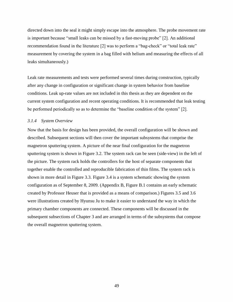
49
directed down into the seal it might simply escape into the atmosphere. The probe movement rate
is important because ―small leaks can be missed by a fast-moving probe‖ [2]. An additional
recommendation found in the literature [2] was to perform a ―bag-check‖ or ―total leak rate‖
measurement by covering the system in a bag filled with helium and measuring the effects of all
leaks simultaneously.)
Leak rate measurements and tests were performed several times during construction, typically
after any change in configuration or significant change in system behavior from baseline
conditions. Leak up-rate values are not included in this thesis as they are dependent on the
current system configuration and recent operating conditions. It is recommended that leak testing
be performed periodically so as to determine the ―baseline condition of the system‖ [2].
3.1.4 System Overview
Now that the basis for design has been provided, the overall configuration will be shown and
described. Subsequent sections will then cover the important subsystems that comprise the
magnetron sputtering system. A picture of the near final configuration for the magnetron
sputtering system is shown in Figure 3.2. The system rack can be seen (side-view) in the left of
the picture. The system rack holds the controllers for the host of separate components that
together enable the controlled and reproducible fabrication of thin films. The system rack is
shown in more detail in Figure 3.3. Figure 3.4 is a system schematic showing the system
configuration as of September 8, 2009. (Appendix B, Figure B.1 contains an early schematic
created by Professor Heuser that is provided as a means of comparison.) Figures 3.5 and 3.6
were illustrations created by Hyunsu Ju to make it easier to understand the way in which the
primary chamber components are connected. These components will be discussed in the
subsequent subsections of Chapter 3 and are arranged in terms of the subsystems that compose
the overall magnetron sputtering system.

50
Figure 3.2: View of entire system (rack, computer and sputter system)

51
Figure 3.3: Control Panels and power supplies for system components
At the very top right: Interlock switch for
main chamber pressure and substrate
heater
Top shelf (from l to r): matching network
and RF power supply
Next shelf (from l to r): TMP 361C and
150 TMP controllers, respectively.
Third shelf: QCM controller and
Baratron controller (which controls
CM#1 and CM#3)
Fourth shelf (from l to r): Gate Valve
(GV) controller (connected to CM#2)
and the MFC controller/readout
(connected to Ar and O2 MFCs)
Fifth shelf: Hot ion gauge controller plus
blank slots (and 1 interlock)
Sixth shelf: DC power supplies (1 shown,
2 planned)
Seventh shelf: Solenoid valve control
box (and built-in power supplies)
Bottom shelf: Substrate rotation
controller and Substrate Heater controller
Very bottom: Surge protectors
Not shown: Connections to PC
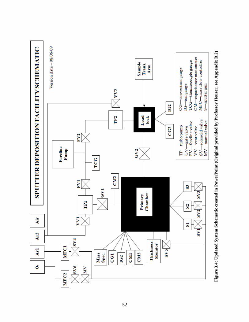
52
Fig
ure
3.4
: U
pd
ate
d S
yst
em S
chem
ati
c cr
eate
d i
n P
ow
erP
oin
t (O
rig
ina
l p
rov
ided
by
Pro
fess
or
Heu
ser,
see
Ap
pen
dix
B.2
)

53
Fig
ure
3.5
: S
ide
vie
w o
f m
ag
net
ron
sp
utt
erin
g s
yst
em (
Ea
rly
ill
ust
rati
on
pro
vid
ed c
ou
rtes
y o
f H
yu
nsu
Ju
)
TO
P
BO
TT
OM
Bo
ttom
of
Sp
utt
er S
ou
rce
Fla
ng
e

54
Fig
ure
3.6
: T
op
-dow
n v
iew
of
spu
tter
ing
sy
stem
(a
lso
pro
vid
ed b
y H
yu
nsu
Ju
)
FR
ON
T
RE
AR

55
3.2 Substrate Selection
The importance of the substrate morphology and lattice structure in determining film quality was
already explained in Chapter 2. This section explains what substrates were selected for the
purposes of urania and ceria film production and how the substrates were prepared for film
growth.
3.2.1 Substrate Selection
Substrate selection is absolutely critical in terms of promoting good film quality. ―In general, if
the lattice mismatch‖ between the substrate and the growing film is large, ―the interface will
have ―a high density of dislocations and the resulting film will be polycrystalline‖ [2]. The lattice
constant (i.e. the length between unit cells of the lattice) of the substrate and the film material is
used to determine the lattice mismatch, often in terms of a percent difference as compared to the
lattice constant of the film. Both CeO2 and UO2 have FCC (or face-centered cubic) crystal
structures with lattice constants of 0.5411 nm and 0.54704 nm, respectively [7, 8]. The two
substrates chosen for use in the system, as of the writing of this thesis, were sapphire (or
corundum) and strontium titanate (or STO). The chemical formulas are Al2O3 and SrTiO3,
respectively.
Sapphire ―has a trigonal crystal structure … in which the oxygen atoms form a hexagonal close-
packed‖ (HCP) structure. However, using the )0211( r-plane of the crystal provides a ―pseudo-
rectangular‖ lattice with constants of 0.512 and 0.4758 [7]. For ceria this represents a mismatch
of 5.4% and 12.1% and for urania this represents a mismatch of 6.4% and 13%. For both film
materials, the mismatch applies a compressive stress to the growing film. The stress is
anisotropic in nature with more stress being applied along the direction of the greater mismatch.
Note that this mismatch is only for the sample at room temperature. As the substrate is heated,
the bombarding particles will have adatom mobility and the mismatch will play a less significant
role. Additionally, the thermal expansion coefficients of the compound and the substrate will
may significantly alter the degree of the mismatch. (This effect is considered beyond the scope of
this thesis as the thermal expansion coefficient of urania would be a discussion unto itself given
its complex temperature dependence.) However, to compensate for the lattice mismatch, sapphire

56
substrates provide ―highly polished surfaces‖ with ―good mechanical strength‖ that are also
―chemically stable in oxygen atmospheres at elevated temperatures‖ all at a low cost [9].
The alternate STO substrates had not yet been used as of the time this thesis was written but had
been used to produce ceria films samples in the MBE system at the UIUC Materials Research
Laboratory (MRL). STO has a perovskite crystal structure however the ―oxygen sublattice‖ (and
thus the oxygen terminated surface) has a FCC structure [10]. If oriented such that the oxygen
lattice is rotated 45° with respect to the deposited film, a SrTiO3 (100) substrate can have a
mismatch of 2.1% with respect to ceria and a mismatch of less than 1% for urania [3, 10].
However, the other properties of the STO substrate are not necessarily as favorable as that
sapphire. The fabrication of the substrates can be difficult.
All substrates used must be single crystal in nature in order to allow the possibility of producing
epitaxial films via magnetron sputtering. Additionally, they must be produced with a small
miscut angle in order to ensure good interface formation. (The miscut angle is the physical
difference between the substrate surface and the actual crystallographic plane.) If the miscut
were large it could interrupt the formation of monolayers as they form on the substrate surface.
The batches of substrates used for the research to which this system pertains have undergone
XRD analysis to verify the miscut. The miscut was found to be less than 1° (with respect to the
offset of the cosine distribution produced via diffraction) and should not affect film formation.
Polishing of the substrate can reduce the substrate miscut (if performed properly) and can also
promote a smoother surface morphology for the substrate. (However, polishing may also
introduce additional stress in the substrate surface that may need to be later relieved by annealing
in-chamber.)
3.2.2 Substrate Preparation
The selected substrates are carefully and rigorously prepared to eliminate surface contamination.
First the substrate is washed in ultrasonic bath of trichloroethylene (TCE), is an industrial solvent
used to remove organic compounds. (The ultrasonic bath serves to agitate or accelerate the
bombardment of the liquid particles with that of the substrate surface increasing the effectiveness
of the cleaning. This would also serve to remove any surface particulates.) The TCE is handled

57
with extreme care as it is a dangerous carcinogen. After the TCE is used the sample is rinsed in
de-ionized water (or DI). It then undergoes another ultrasonic bath in a different solvent,
concentrated acetone. This is used to remove other (potential) organic compounds that may be on
the film surface. Another rinse is performed (if necessary). Any residue from the acetone bath is
removed by using an ultrasonic bath of isopropyl alcohol (IPA). Finally, the substrate is cleaned
in a bath of methanol. Methanol evaporates very quickly and also serves to remove any adsorbed
water from the surface of the substrate. (Care must be taken not to allow water to enter the
squeeze bottles of the methanol; it will dilute the methanol and reduce its effectiveness in
removing water.)
After the substrate has been cleaned it is affixed or bonded to a roughened Inconel sample holder
with low vapor pressure silver thermal paste. (The sample holder was originally smooth but was
roughened with fine grit sand paper to increase the surface area to which the thermal paste could
attach thus binding the substrate to the sample holder more securely.) The thermal paste must be
cured over a period of several hours in which the temperature of the sample holder is increased
to a few hundred Celsius using a resistive heated hot plate. Curing the paste not only guarantees
a more secure bond, it also allows for a greater thermal conductivity between the sample holder
and the substrate. The curing process may also serve to alleviate some stress that may be present
in the substrate by mildly annealing it.
All told, substrate and sample preparation takes almost a full work day to complete. For this
reason a second Inconel holder was purchased to allow one holder to be prepared while another
is being used for film fabrication. Note that during all preparation steps powder-free disposable
nitrile gloves are worn and the sample is only held using plastic tweezers or with a particle-free
KimWipe. Additionally, the substrate surface can be blown clean with high purity Argon gas to
remove particulates as necessary. A final wipedown with methanol and a KimWipe is performed
before the sample is introduced into the load-lock.

58
3.3 Fixturing and Sample Manipulation
The system was designed as a two-chamber system to decrease the possibility of system
contamination and to increase reproducibility. This section will be devoted to the fixturing and
process by which samples are transported to and mounted in the processing chamber. It will then
cover the range of options that the sample stage affords once the sample has been mounted.
3.3.1 Sample Transfer Apparatus
Fixturing (or fixtures) ―can be defined as the removable and reusable structures that hold the
substrates, and tooling can be defined as the structure that holds and moves the fixtures and
generally remains in the system‖ [2]. The substrate is attached to the sample holder as described
in the previous section. The sample holder is shown in Figure 3.7 and is loaded onto the sample
transfer plate shown in the load-lock (shown in Figure 3.8). The three pins lock into the
corresponding holes in the sample holder. The sample holder is placed face down (or back-side
up). The load-lock is then closed and evacuated. Once the vacuum has reached a suitable level,
the manual gate valve is opened and the sample holder (and sample plate) is transported into the
main chamber. Figure 3.9 shows the magnetically-coupled transfer arm used to provide the linear
motion for the sample transfer plate. The transfer arm uses the black sliding magnetic
manipulator shown on the exterior of the arm to manipulate a corresponding magnetic slider on
the inside of the sealed arm. Thus the rod (or feedthrough internal to the arm) can be rotated or
slid in horizontal motion without compromising the vacuum of the load-lock.
Once the plate is position beneath the center of the transfer stage (at a height in between that of
the base of the stage and the main shutter) the central shaft of the stage is lowered by hand using
a rotary feedthrough. This post has three fin-like projections that slide into and ―lock‖ into the
three cut-outs that can be seen in Figure 3.7. The post is then raised (by rotation in the opposite
direction) and the sample holder is lifted off the transfer plate. The plate can then be removed by
sliding the transfer arm in the reverse direction as before. The manual gate valve is then closed
isolating the main chamber and allowing it to return to a suitable vacuum before film fabrication.
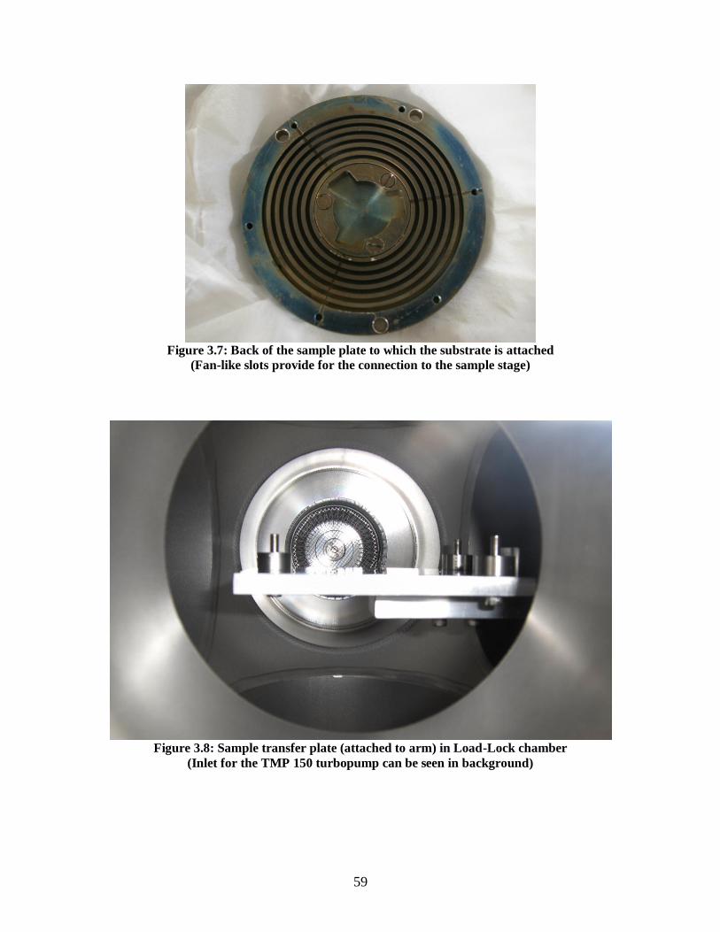
59
Figure 3.7: Back of the sample plate to which the substrate is attached
(Fan-like slots provide for the connection to the sample stage)
Figure 3.8: Sample transfer plate (attached to arm) in Load-Lock chamber
(Inlet for the TMP 150 turbopump can be seen in background)

60
Figure 3.9: Sample Transfer Arm
3.3.2 The Sample Stage, Sample Rotation and Sample Heating
Once the sample is mounted to the sample stage (as described previously), the sample may be
rotated, heated and have its vertical position adjusted. The aforementioned manual rotary
feedthrough can then be used to adjust the vertical position of the sample holder by a few inches.
As discussed in Chapter 2, the vertical position of the sample affects the angle-on-incidence of
the impinging flux as well as the degree to which it is thermalized based upon the distance the
particles must travel. The rotary feedthrough is positioned such that if ―wear particles‖ were to
be generated they would fall onto the back of the sample holder. This prevents contamination of
the substrate and the sputter targets.
Sample rotation is used for to produce ―position equivalency‖ so that the substrate is subject to as
uniform a flux as possible. (Practically speaking, this is of course limited as the center of the
substrate will see a different flux as compared to the edges. However, the edges should see the
same amount of flux as each other because of the rotation.) The speed at which the sample
rotates can be controlled by the controller shown in Figure 3.3.

61
The substrate heater is used to heat the sample holder and thereby the substrate (assuming good
thermal conductivity) up to a maximum temperature of 850°C. (For comparison purposes, the
melting temperature of UO2 is 3120 K [11]. Thus the substrate heater would allow a maximum
substrate temperature to compound melting temperature ratio of 0.36. As documented in Chapter
2, this would allow films to be grown in the region between Zone 1 and Zone 2, also known as
the Zone T growth mode.) The substrate heater functions by using two halogen bulbs placed in
front of a parabolic reflector to radiatively heat the back of the sample holder. The bulbs are
protected by a transparent quartz disk and the sample stage is cooled by water coolant provided
through ¼ in. steel tubing internal to the vacuum chamber. The temperature in the sample holder
is measured using a standard thermocouple gauge that makes contact through the connection to
the sample stage. (This also allows any additional of sample holder, perhaps by energetic
bombardment, to be accounted for.) Figure A.3 shows the sample holder as it is cooling (after it
has been heated to 850°C and the heater has been turned off).
As an alternative to a thermocouple gauge, an infrared pyrometer was considered. ―Infrared
pyrometers allow determination of the temperature if the surface emissivity and adsorption in the
optics is constant and known‖ [2]. This would have simplified the sample stage design, but
would have increased the complexity of the chamber design by requiring an extra port being
welded to the chamber. As the sample stage which was purchased naturally included the
electrical feedthroughs for a thermocouple, the pyrometer was rejected.
Additionally, a voltage bias may be applied to the sample holder and (thus the substrate if it is
conductive) by the physical connection between the sample stage post and the holder. No other
connection is possible because the fixture is also rotating. The large contact area provided by the
three fins (or fan blade like projections) allow for large currents to be applied if necessary [2].
This should allow the bias on the sample holder to significantly affect the flux of incoming
charged particles. (This is important if the substrate selected is nonconductive because the bias
will not be applied directly to the substrate.) If there is a concern about good electrical contact,
an ―electrically conducting anti-seize lubricant such as a metal selenide‖ may be used [2]. (This may
also make removal of the sample holder from the rotating shaft blades easier.) As discussed in

62
Chapter 2, applying a voltage bias may be used to increase film quality and can sometimes be
used to preferentially grow crystallographic orientations in films, such as ceria [2].
3.3.3 Sample Mask
Another system component that could be considered tooling or fixturing is the ―sample mask‖ or
simply ―mask.‖ The sample mask has yet to be installed but would be used to obfuscate or block
the sample holder (or plate) so that the sputtered material only lands on the substrate. This is
done for primarily practical reason as it means there is less material that needs to be cleaned off
the sample holder after film production. (Typically, the sample plate is simply scraped clean with
a razor blade and then cleaned with solvents before it is given a final wipe down with methanol.)
However, when producing uranium-based films this mask serves the additional function of
limiting radioactive contamination. The urania that coats the mask (instead of the sample holder)
remains in the chamber thus reducing exposure to the outside environment.
When designing a mask it is important to account for substrate size, position and the angle-of-
incidence of the sputtered material. Usually the mask is located as close to the sample holder as
possible. The simplest design of a mask calls for a thin metal sheet with a cut-out corresponding
to the shape and size of the substrate. The size of the hole can be further reduced by accounting
for the angle-of-incidence of the incoming particles and the distance between the sample and the
mask. (This is because the particles ―spread out‖ after passing through the mask before
depositing on the substrate.) The design of the mask should never compromise film uniformity
and position equivalency techniques such as sample rotation should still be used.
Ideally, the mask would rotate freely with the sample holder. This would allow the cut-outs in
the mask to be the same shape as the substrates to be deposited upon. However, this greatly
increases the complexity of the design as the rotation is provided by the support fixture that holds
the sample plate. Some means would have to be devised to attach the mask to the sample plate as
it enters the chamber, but this would further complicate sample loading procedures. Preliminary
mask designs call for the mask to operate like a shutter. This allows for easier loading of the
sample holder. (Alternatively, it is still possible to have the mask as an independently supported
fixed object in the chamber, but this increases the complexity of loading the sample by reducing
the volume in which it can be maneuvered.)

63
The preliminary mask design has a circular hole cut-out so as to account for the rotating square-
shaped substrate mounted to the sample. The mask would attach to the same rotating post to
which the main shutter is currently connected. (As the shutter moves out of the way the mask
slides into place.) This design is illustrated in Figure 3.10 (a). The author has also suggested a
possible alternative mask in Figure 3.10 (b) that incorporates a shaped baffle so as to block the
oblique component of the flux from depositing on the substrate. (Note that the size of the baffle
is exaggerated in the image as it is merely provided to serve as a conceptual image.) As noted in
Chapter 2, the use of a baffle could be used to account for a high processing pressure (or to
reduce a high sputter rate). The exact shape, length, and angle of the baffle could also be tailored
the position of the sputter source as it relates to a specific substrate position (e.g. for a given off-
axis position or specific height).
Figure 3.10: Sample mask designs: (a) standard and (b) with cylindrical baffle for collimation
(The size of the baffle has been exaggerated and the position is not final) (Created in PowerPoint)
3.4 Magnetron Sputtering Subsystem
The magnetron sputtering system provides the solid material to be sputter deposited onto the
substrate. This section will detail the selection of components and the configuration of these
components.
3.4.1 Magnetron Sputtering Guns and Target Configuration
―The geometry of the sputter deposition system determines many of the factors that affect the
properties of the deposited film and the throughput of the system‖ [2]. Many of these factors
have been discussed in previous sections or chapters, yet there are also more obvious practical
design considerations that are determined by the use of a sputter system. Sputtering allows for
(a) (b)

64
the overall system to be much more compact and for the target to substrate distance to be
smaller. This is because the sputter sources operate at lower temperatures and cause less heating
than would be found in a vaporization based system (like an MBE system) [2]. A smaller volume
system will have less space to be evacuated and less surface area for contaminants to adsorb
onto. This decreases pump down time and makes it easier to maintain high system purity.
A magnetron sputter system also provides for co-deposition of films by using multiple
magnetron guns spaced closely together. The three magnetron guns are shown in Figure 3.11.
The ―arrangement approximates a cylindrical target and allows a more uniform distribution of
incident flux on an object placed at the center‖ or focus of the slightly angled magnetron guns
[2]. (Note that the vertical position of the sample can be adjusted so that it is at the focus of the
three guns.) Each magnetron has its own shutter so that it will be protected from sputtered
material when not in use.

65
Figure 3.11: Active argon plasma and substrate heater as seen from main viewport
(For scale purposes a sample substrate may be seen on top of the primary shutter)
Note in Figure 3.11 the shutter is open on magnetron gun 3, and there is an active plasma on the
Cerium target. Additional light in the chamber is provided by the substrate heater. (The sample
holder is in a raised position so it is harder to see.)

66
Figure 3.12: Magnetron guns with the corresponding pneumatic valves, gas lines, and coolant lines
3.4.2 Sputter Targets
The targets themselves are simply 3-inch (diameter) disks of the chosen material. Sputter targets
are ―long-lived sources‖ ideal for two-chamber PVD systems where the main chamber should be
open to the ambient as infrequently as possible for maintenance [2]. The targets used in the
system are minimum ―three nines‖ purity (or 99.9% pure). (Note that the manner in which the
targets are manufactured can determine their purity, density and porosity—all of which are
interrelated. For example, sintered targets are less dense and therefore may outgas more and be
more porous once the outer layers have sputtered off [2].) To prevent overheating (and melting)
of the targets the magnetron guns are actively cooled. To increase heat removal, the targets are
typically screwed or bonded to a copper backing place. The uranium and cerium targets are both
brittle causing the threads to break off thus detaching the targets from the copper plates unless
bonded with thermal compound. Alternatively, if the guns are operated at a low enough power,
the targets can be placed in the guns without a backing plate. However, the choice of power
supply can also affect this decision. For example, RF power supplies can cause non-conducting
materials to heat rapidly.

67
Heating of the targets can cause them to expand slightly, but the greatest change in the target
shape is from sputtering. ―In planar magnetron sputtering the target develops a ‗racetrack‘
depression on the surface. This changing geometry can affect the deposition rate, vapor flux
distribution, and other deposition parameters such as the amount of reactive gas needed for
reactive deposition in reactive sputter deposition‖ [2]. Typically, only a fraction of the sputter
target (usually ―10 to 30 percent‖) is used as the ―racetrack erosion‖ determines the overall
―lifetime‖ of the target [2]. This time can be increased by removing the target and melting it so
that the surface becomes uniform once more. However, this can introduce impurities into the
target and it is usually simpler and more cost effective to buy a new target.
Another consequence of sputtering the target is that they may become coated in a thin ―‗smut‘ of
fine particles.‖ These particles may result from poisoning of the target, gas-phase nucleation, or
―cross-talk‖ with other sputter guns (where there material is deposited on another nearby target).
These particles can be simply wiped off during maintenance or can be cleaned in system using
―pre-sputtering‖ [2]. Pre-sputtering is simply sputtering of the target for a given length of time
while the substrate is shielded by a shutter or held in the load-lock chamber. Sputtering removes
adsorbed contaminants from the surface of the target and is most commonly used to remove any
excess compound created by the reactive gas. It is important to note that the surface morphology
of a sputter target can affect the morphology of a sputter deposited film. A smooth, clean sputter
target will produce a more uniform flux of sputtered atoms. Therefore the target should always
be pre-sputtered before film fabrication and for an increased time after system maintenance that
involves opening the main chamber.
3.4.3 Power Supplies
The magnetron guns can be powered (i.e. have the electric potential produced) by either a DC
power supply or a RF power supply. In order to have ―reproducible sputtering parameters‖ ―the
target power (watts/cm2) and voltage‖ must be monitored. ―In the case of rf sputtering, the
reflected power from the target is measured and controlled by the impedance matching circuit‖
[2]. The power supplies used have built in readouts and can be controlled by means of the
voltage, current and/or total power. The RF matching network for the RF power supply is a
separate component located on the system support frame and requires the use of a copper
grounding strip. The DC supplies have built-in arc suppression circuitry.

68
There are currently a total of three power supplies; two DC power supplies and one RF power
supply. This allows for all three guns to be operated simultaneously or for two guns to be
operated while a voltage bias is applied to the sample holder (and substrate). Each type of power
supply has its own advantages and disadvantages. RF power supplies are more complex than DC
supplies and require the use of an impedance matching network to maintain a constant net
voltage. (By net voltage it is meant to mean the average voltage at which the RF signal oscillates
above and below.) RF power can also ―creep‖ along metal surface and can present a hazard
unless the system is properly grounded.
Nevertheless, there are distinct advantages to RF supplies. RF can be used to activate a plasma at
pressure lower than 1 mTorr (given the right geometry and gas flow). (This is lower than what
DC supplies are generally capable of because there plasma may be less dense for a given power
level.) They also prevent charge build-up on the target surface (as noted in Chapter 2), this
reduces the chances of ―poisoning the target‖ with too much reactive gas or of causing arc
formation on the surface of the target. (Arcing can damage the magnetron guns and most
supplies are built with arc suppression circuitry.) Finally, although this is not currently a feature,
both an RF and DC potential can be applied to a single target (as long as there is a RF choke in
the DC circuit to prevent damage of the power supply) [2]. This technique will increase the
plasma density along the target surface and will be discussed further in Chapter 4.
3.4.4 Quartz Crystal Monitor
Finally, there must be a means of determining the amount of material sputtered from the target
and deposited onto the substrate. To do this the deposition time is recorded and the deposition
rate is measured using a quartz crystal deposition monitor or QCM for short. A QCM is a real-
time in situ monitor that functions by applying a voltage at a high frequency (usually around 5
MHz) to a piece of single crystal quartz. Because the quartz is a piezoelectric material, the
applied voltage causes the volume of the crystal to increase. Since the voltage is applied at a high
frequency the crystal resonates with a frequency that is determined by the magnitude of the
voltage, and the crystal properties. As material deposits on the quartz, the resonance frequency
decreases proportionally to the amount of mass added. It is this frequency change that is used to
determine the amount of film deposited onto the QCM and, indirectly, the amount deposited onto
the substrate. [2]

69
In order to approximate the film deposited onto the substrate the QCM must be calibrated. First,
the density of the material deposited must be input into the QCM controller then the z-factor
must be entered. The z-factor is the ratio of acoustical impedance of the film material to that of
the quartz crystal. (Again, crystal properties such as its crystalline orientation affect this value.)
It should also be noted that heating of the QCM due to high deposition rates may affect the
resonance and artificially alter the deposition rate. This can be accounted for by applying coolant
to the QCM (which is an optional feature of the system). Another factor which may affect QCM
accuracy is film stress of the film on the crystal. (This effect can only be calculated by
comparing the deposition rate to a different QCM with a different crystal orientation.)
Finally, a tooling factor must be determined experimentally that correlates the amount of
material deposited on the QCM with the amount on the substrate for a given time. (The amount
of material will be calculated by the QCM controller and the amount on the substrate will have to
be determined using one of the techniques described at the end of Chapter 2. The resulting ratio
is then the tooling factor.) The tooling factor for the system will most likely be greater than one
as the amount of material deposited on the substrate will most likely be several times greater than
that deposited on the QCM. This is by design. The QCM was positioned off-axis and at an angle
with respect to the sputter gun so as to reduce the material deposited on the crystal. This
increases the lifetime of the crystal because after a certain amount of material has been deposited
on it the crystal needs to be replaced. It is also important to note that the tooling factor will vary
depending on which gun is used to deposit the material (as the angle is different with respect to
the QCM is different for each).
When co-depositing material the results of the QCM will be less accurate. The only way to
account for this would be to add more QCMs to different locations in the chamber or to use an
alternative method of deposition rate monitoring. Other methods researched included ionization
deposition rate monitors and optical adsorption spectrometry (AAS) based monitors. Both of
which would require altering the system geometry and would be calibrated only for the particular
depositing material (and a fixed geometry). These costly alternatives were eliminated and only a
single QCM system was implemented. The use of a single QCM greatly simplifies the overall
system design while still allowing the approximate amount of material deposited to be

70
determined during sputtering. All samples produced in the system will be characterized fully;
this includes the depth profile of each sample to determine the final, exact thickness.
3.5 Gas Distribution System
The gas distribution system consists of a (vacuum) chamber, a pump for evacuating (or reducing
the pressure of) the chamber, a means of measuring and introducing gas into the system, and a
means of measuring and controlling the overall pressure in the chamber. The basic design
decisions involved in developing the gas distribution system will be detailed in this section.
3.5.1 Pumping System Design
The level of cleanliness desired for a particular process determines the vacuum range at which a
system is required to operate. By extension it determines the type of vacuum pump or pumps
required to achieve and maintain the vacuum. As noted in Chapter 2, the system was designed to
attain a ―base pressure‖ in the 10-7
to 10-9
Torr range (or a ―very high vacuum‖). Figure 3.13
shows different vacuum pump operating ranges. The lower the pressure (or higher the vacuum)
required the greater the price of system components and the higher the degree of system cleaning
and preparation required.
Figure 3.13: Vacuum pump operating ranges (in Torr and Pascals) [3]
Based on this figure, a turbomolecular pump backed by a secondary pump would be the best
solution to achieving the desired vacuum (and the most cost effective when compared to exotic
solutions such as cryopumps or ion pumps.) The primary (turbomolecular) pump selected was a

71
Oerlikon Leybold TMP 361C. It is rated at a pump speed of 350 L/s for Argon gas and is
compatible with corrosive environments. (The corrosion resistance was deemed an important
feature as the reactive gas being used in film fabrication is pure oxygen.) The pump speed
criterion was based on the original design specs for the magnetron system which was a 6-inch CF
cross. A pump speed of 350 L/s was determined to deliver optimal performance at a competitive
cost. When the system was redesigned to accommodate a 10-inch CF spherical cross this pump
speed was still deemed adequate.
Figure 3.14: CF turbopump (with cut-out) and Sectional view of turbopump blades [12, 3]
―The turbomolecular pump or ‗turbopump‘ is a mechanical type momentum transfer pump,‖
sometimes referred to as a ―capture pump,‖ because its ―high speed vanes impart momentum to
the gas molecules‖ effectively forcing the molecules to proceed through the pump and out of the
system. (It is important to understand ―that the molecules are not actually attracted by the pump
but rather that they move freely through the system until they, by chance, find a pump which
―traps‖ them or provides them with a preferential flow direction. Thus a vacuum pump is a
device that takes a gas or vapor atom/molecule that enters it and prevents it from returning to the
processing chamber.‖) [3, 2]

72
The turbopump requires ―very close tolerances in the mechanical parts and cannot tolerate
abrasive particles or large objects‖ thus it was positioned to minimize the amount of debris it
would encounter due to film fabrication [2]. The TMP also uses magnetic bearings in order to
avoid the use of lubricants in order to increase system purity. In this system, the turbopump is
―rough-pumped through the turbopump as it is accelerating‖ [2]. This means a secondary pump
lowers the system pressure to a low enough pressure that the turbopump may begin to operate by
evacuating large quantities of gas through the turbopump while it is off. (Typically, the pressure
must be less than 100 mTorr for a turbopump to begin operating. Like most vacuum components,
over-pressurization may damage the turbopump if it is active.) This pump is also used to exhaust
to atmosphere as a turbopump is incapable of exhausting to such a high pressure.
The secondary pump, often called a roughing pump because it lowers the system to that of a
―rough vacuum,‖ used in the system is a Trivac D 25 B pump (also from Oerlikon Leybold).
This is a direct-drive two-stage rotary oil-sealed mechanical pump. ―Mechanical pumps are
positive displacement pumps that take a large volume of gas at low pressure and compress it into
a smaller volume at higher pressure‖ [2]. The oil in the pump is used to ―seal‖ or maintain a
vacuum in the pump. The oil must be filtered or replace every few months. Typically this oil is a
semi-viscous hydrocarbon oil (that may need to be heated with a sump heater during start-up.
Otherwise, if the surrounding environment is too cold, the roughing pump will trip). However,
because oxygen is being used as a reactive gas for processing, alternative non-hydrocarbon oils
may be used to in order to prevent oil degradation and potential flammability. These oils are
typically ―perfluorinated polyethers‖ (PFPEs), one particular brand considered for use was
Fomblin pump oil. Although these pump oils increase safety by providing greater ―chemical
stability,‖ they significantly reduce pump performance by providing less lubrication and
requiring greater heating in order to maintain a low enough viscosity. It was deemed that the O2
levels were significantly low to preclude an explosion and that the dramatic increase in cost
(over an order of magnitude) in using PFPE was unjustified.
One additional design consideration when using a roughing pump is the possibility of back-
streaming. Back-streaming occurs when the roughing pump is pumping down on a chamber
lower than the pressure generated by the pump itself (i.e. below its operational range). The gas

73
within the roughing pump (including oil vapor) can backstream into the volume at reduced
pressure thus contaminating it. This situation would occur if the turbopump were to accidentally
trip (or shut off) and the roughing pump is pumping on already evacuated chamber. To prevent
this, a series of two oil traps was installed. The first trap uses standard copper gauze to trap the
oil. This eliminates over 90% of oil and needs to be replaced every few months, depending on
use. The second trap in the series was a high-efficiency aluminum oxide pellet trap that
eliminates 99.9% of oil. The pellets need to be replaced every three months. The oxide pellet
based filter is shown in Figure 3.15. (Additional methods to prevent backstreaming in the case of
an accident scenario are discussed in the maintenance and support subsection.)
Figure 3.15: Oil Trap with aluminum oxide pellets and insert [13]
Finally, as an aside, if one wanted to increase the system purity significantly at low cost they
could add a means of adsorption pumping to the system for the purposes of removing
condensable contaminants such as water vapor [2, 3, 14]. This would be particularly effective in
this system in its current configuration because ―turbopumps have poor pumping ability for
water vapor since the water molecules must make many adsorption-desorption events to pass
through the pump‖ [2]. However, the improvement in base pressure is directly dependent on the
amount of water vapor in the system (and its corresponding partial pressure) and the surface area
of the cold trap relative to the system volume [14]. The effective pumping speed of a liquid
nitrogen (LN2) cold-trap is given by:
where S is the effective pumping speed, A is the surface area of the trap, and v is the average
velocity (or thermal velocity) of water particles in the system [14]. (Concepts such as pumping
speed and average velocity will be discussed in greater detail in Chapter 5.)
42
AvSLN

74
A pump is connected to a vacuum chamber either directly or by means of pipework referred to as
the pumping stack. Additional design modifications had to be made to the pumping stack in
order to accommodate a 6-inch (O.D.) CF turbopump and the primary chamber which was
simply a 10-inch (O.D.) 6-way steel cross. A 10-inch to 6-inch reducing nipple was added to the
back ―leg‖ of the chamber to account for the change in diameter. A cross was then added in order
to provide two ports for adding instrumentation. At this time, the top port is used to connect one
of the .02 Torr Baratron gauges and the bottom port is blanked (or sealed) off. The GV was
placed between the cross and an elbow so as to control the conductance of the pumping stack.
(This is discussed in detail in a later subsection.) The elbow was used as part of the pumping
stack to offset the pump and eliminate a direct line of sight between the pump and the magnetron
guns. This was done to minimize the amount of sputtered material (or debris) that could enter the
pump and possibly damage it. (Note that in its current configuration it is still possible for
particles to deposit on the inside surface of the elbow and then later fall down into the pump.
However, the pump also has a small screen at its entrance which may prevent some physical
matter form entering it. Conversely, this screen has the potential to reduce the effective pumping
speed of the pump, especially if it becomes heavily coated.) The placement of the pump was
chosen so as to maximize the design lifetime of the system although it does come at the cost of
the overall conductance of the gas distribution system. The concept of conductance and it affect
on the system will be discussed further in Chapters 5 and 6.
3.5.2 Pressure Measurement and Pressure Control using the Gate Valve
Several types of pressure sensors are used in this system design. These sensors function based on
different methods which determine the range of operability and are described in Table 3.1.
Table 3.2: Pressure Ranges of various vacuum gauges [3]

75
An analog thermal couple (TC) gauge is used to measure the vacuum pressure in the roughing
lines (or foreline) connecting the roughing pump to the turbopumps. This is used to verify that
the roughing pump is operating nominally and that backstreaming cannot occur in the line. (Its
operation pressure range is valid from a few mTorr up to atmospheric pressure.) A pirani gauge
is also available (in conjunction with the mass spectrometer) to allow for gas measurements at
intermediate pressures in the system.
Hot cathode ion gauges are used to measure overall system pressure when pumping down on the
chamber as they are accurate to a lower pressure than the other gauges available. Ion gauges use
a constant electrical current to ionize the gas near a helical coil. The charged coil then causes the
ions to be driven toward a ―collector.‖ The ion current is then measured and used to determine
the molecular density of the gas present and thus the system pressure. A hot ion cathode gauge
uses a heated filament to produce more electrons and thus more ions (as compared to a cold
cathode gauge). The greater number ionizations thus allows the hot cathode gauge to operate at
lower pressure (and to be more accurate at the same pressure based on the statistics of having a
larger sample population). However, the hot cathode gauges used in the the sputtering system
must ―warm-up‖ for a minimum of two hours and should also be outgassed periodically to
achieve accurate readings. Condensation of gas on the helical coil can reduce the amount of ions
collected. Additionally, the type of gas ionized may also impact the measurements for some
gauges. As always, contamination should be minimized in the system to facilitate more accurate
and reproducible measurements [2]. (Also note that because the measurements of an ion gauge
are determined based on the ions it produces introduction of foreign ions will induce error in the
readings. Therefore, the ion gauges must be located sufficiently far away from the plasma or out
of its line-of-sight. This has been acknowledged in the design of the system.)
The system uses a series of capacitance manometers (or CDGs) to determine the absolute
pressure of the system. A capacitance manometer contains a metal diaphragm as part of a ―metal-
on-ceramic electrode structure‖ (i.e. a capacitor) that is hermetically sealed with a very high
vacuum (relative to the pressure range at which the sensor is designed to operate) on one side of
the diaphragm with the other side exposed to the chamber conditions. The pressure in the
chamber causes the diaphragm to be deflected which then alters the capacitor (by reducing the

76
separation distance between the metal and the ceramic). The ―pressure is determined by
measuring the change in capacitance between the metal diaphragm and an adjacent, fixed dual
electrode.‖ The inside of a CDG is shown in Figure. 3.16. (The ―internal getter pump‖ is usually
just a chemical reagent insert used to adsorb any of the electrode material that may decay and
outgas in order to maintain the reference vacuum.) [15]
Figure 3.16: Inside of a capacitance manometer [15]
The Baratrons used are two 627B models and one 627D (which is just the most recent iteration
or refresh of the 627B). One Baratron is a 1000 Torr full scale gauge used to verify pressure
when raising the chamber pressure to atmospheric pressure for maintenance. The other two are
.02 Torr gauges (accurate to as low as 2x10⁻⁷
Torr). One is used to control the GV and is located
in the pumping stack. (This is not an ideal situation as this may cause the sensor to be exposed to
additional pressure fluctuations [2], this phenomenon is discussed in detail in Chapter 5.) The
other is used as an independent monitor of chamber pressure and is attached to the cluster flange
on the side of the chamber. (Comparing the two manometers measurements also provides a
means of ―early detection‖ for ―gauge drift‖ so that the gauge in question may be re-calibrated as
soon as possible and the system itself is not considered to be suspect [2].) The manometers are
all temperature-controlled to 45°C (i.e. heated to and matained at said temperature) so that they
are ―less effected by changes‖ in the ambient temperature. Heating also ―reduces the possibility
of process byproducts depositing in the manometer‖ and causing it to drift [15]. Additionally,
―the radially tensioned diaphragm provides very low hysteresis, excellent repeatability,
remarkably high resolution (1x10⁻⁵
of Full Scale), fast response, and the ability to measure
extremely low pressures‖ [15]. Figure 3.17 shows one of the 627 Baratrons.

77
Figure 3.17: Baratron Pressure Gauge [15]
It is important to note that these gauges do not measure the relative pressure that would be seen
at the substrate surface. ―In a sputtering system, pressure differentials can exist in the deposition
chamber‖ such that the pressure at the substrate surface could be significantly different than that
of the chamber as a whole. ―These pressure differentials can be due to the gas injection
manifolding, crowding in the deposition chamber, or position with relation to the pumping‖ stack
[2]. Accounting for this and measuring the local pressure would require a ―nude gauge.‖ (A
gauge, most likely not a capacitance manometer but possibly a viscosity-based spinning rotor
gauge, that would need to be exposed directly to the plasma environment.) [2]
Nude gauges can degrade quickly in a reactive sputter environment and would require frequent
maintenance. They would also require additional feedthroughs in order to be installed (and given
the current geometry of the system, might even necessitate a new port be welded into the
chamber side). As such, the design decision was made not to directly monitor the local pressure
at the site of film fabrication but rather to use the chamber pressure as an operating parameter to
ensure reproducibility. (As long as the chamber geometry and gas flow rate is held constant, than
controlling chamber pressure should also guarantee that the local pressure is also consistent from
run-to-run.)
The GV controller is shown in Figure. 3.18. It can be used to manually control the GV position
or to allow the GV to automatically adjust position so that it ―may throttle the gas flow through
the pumping stack‖ in order to maintain a pre-set pressure [2]. (This process will be described in
greater detail in Chapter 5.)

78
Figure 3.18: Gate Valve Controller [16]
Figure 3.19: The main chamber with magnetrons gun (bottom), main shutter (center), sample
stage/heater (top) and the pumping stack with Gate Valve closed (in background)

79
Figure 3.20: System (side-view) Note the roughing lines and oil traps (in front) and the pumping
stack and turbopump (center-right)

80
Now that the means of evacuating the chamber and controlling pressure have been discussed the
means of introducing processing gases and the other ancillary gas distribution components will
be covered.
3.5.3 Gas Supplies, Mass Flow Controllers, and the Gas Injection Manifold
The reactive gas and the working gas supplies used are ―five nines‖ and ―six nines‖ pure,
respectively (i.e. 99.999% O2 and 99.9999% Ar). Each gas supply used a dual-vane high-purity
all stainless steel regulator valve (specific to that gas/bottle connection). Use of dual-vane
regulators, as opposed to single-vane regulators, allows the gas supplied to remain at a
continuous (non-fluctuating) pressure as long as there is gas available in the tank. The regulators
have stainless steel VCR connections and are connected to lock-in integral VCR valves (which
were cleaned by the manufacturer to clean room standards). The secondary valves then connect
to custom-ordered ¼ in. stainless steel piping with VCR connections that were bent into the
desired shaped using a pipe bender. These metal gas lines transport the gases to their respective
Mass Flow Controllers (MFCs). The tanks and associated valves and piping are shown in Figure
3.21. (The processing gases are the two smaller tanks to the left.) The MFCs are shown in Figure
3.22 (to the left). Note that for safety purposes, the O2 line also has a flash suppressor so that if
flammable gas were somehow introduced into the line and ignited it could not back flow into the
O2 tank. Additionally, the regulators only allow pressures of up to 30 to 40 psi. This is
intentional so that the gas lines cannot become over-pressurized. (Over-pressurization would
damage the MFCs; safety could be further enhanced by adding a pressure relief valve and flow
restrictor, in-line, before the MFC [2].)
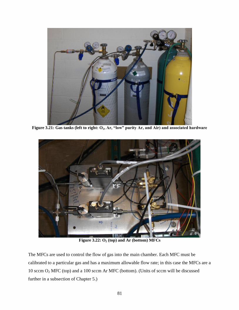
81
Figure 3.21: Gas tanks (left to right: O2, Ar, “low” purity Ar, and Air) and associated hardware
Figure 3.22: O2 (top) and Ar (bottom) MFCs
The MFCs are used to control the flow of gas into the main chamber. Each MFC must be
calibrated to a particular gas and has a maximum allowable flow rate; in this case the MFCs are a
10 sccm O2 MFC (top) and a 100 sccm Ar MFC (bottom). (Units of sccm will be discussed
further in a subsection of Chapter 5.)
82
MFCs are a combination of a mass flow meter and metering valve. The mass flow meter operates
by taking a percentage of the gas flowing through the MFC and channeling it so that if flows
across a heated element. The power needed to maintain the element at a constant temperature is
measured and used to determine the gas flow based on the thermal conductivity of the gas [2].
(This is why the MFC must be calibrated for a particular gas.) ―The cooling rate also depends on
the amount of turbulence in the gas flow,‖ this is the reason why MFCs are designed for specific
mass flow ranges [2]. The output measured by the meter in the MFC is then used to control a
mechanical actuator (which functions as a metering valve). This metering valve is not intended
to function as a shut-off valve. As such, each MFC used in the system has its own pneumatic
shut-off valve. (These are the silver cylinders next to the black rectangular MFCs in Figure 3.23.)
(Note that Fig 3.23 is a picture of an older configuration. In the most recent update, another
manual integral release valve has been added so that the O2 line may now connects to the Ar gas
manifold if desired. This allows for gas mixing in the lines before introduction into the chamber.)
Figure 3.23: Mass flow controller (MFC) with shut-off valve [17]
The MFCs are connected to a readout located on the instrumentation rack (Figure 3.3). The
readout takes the voltages output from the MFC and translates it so that the gas flow is displayed
in terms of sccm. The readout can also be used to ―set‖ the MFC at a given flow rate so that they
will automatically adjust themselves to maintain this flow rate.
Figure 3.24: Readout [18]
83
As discussed in Chapter 2, the availability of reactive gas and the partial pressure of the gas are
important considerations in reactive deposition. Typically, the ratios of the flow rates input into
the MFC Readout can be used to determine the partial pressure as long as the total system
pressure is known. (This is the case as long as ―the system has a constant pumping speed for
each of the gases being used.‖ This is basically true for the case of Argon and Oxygen based on
the pump curve in Figure 5.11.)
Dalton‘s Law was developed from the Ideal Gas Law, which will be detailed in Chapter 5, and
explains that the pressures contributed by individual gases in a chamber are called partial
pressures and when summed they must equal the total pressure of the system.
...321 kTnkTnkTnnkTPt
...321 PPPPt
This makes it very simple to estimate the initial partial pressures of gas introduced to the system
as they will correspond to the ratio of gases delivered via the programmed MFCs multiplied by
the total chamber pressure. However, as noted in Ch. 2, in order to account for gettering of the
reactive gas due to film fabrication an alternative means must be used to measure the relative
amounts of the gases. The mass spectrometer is best suited to this task.
―In-chamber gas composition monitoring can be done with a differentially-pumped mass
spectrometer;‖ however, it can ―only analyze the gas mixture at a certain place in the chamber
and variations with position are difficult to determine‖ [2]. (As noted earlier, this is the same
case with pressure sensors.) As such, for the purposes of reproducible fabrication, only the mass
flows from the MFC Readout and the total pressure measurements for the Baratron gauges will
be used as process metrics. In its current position (located off of the cluster flange near the O2
injection port), the mass spectrometer will only be used to estimate the ratio of contaminant
vapors to that of the processing and working gas in the main chamber. Note that optical emission
monitors or adsorption spectrometers may be used in place of a mass spectrometer but were not
due to their increased complexity and the difficulty involved in attaching them directly to the
main chamber.

84
The ―amount of reactive gas available for reaction in the chamber will‖ also depend on ―factors
other than the mass flow into the chamber.‖ ―These factors include the deposition rate and the
area on which the film is being deposited‖ and ―the way the reactive gas is introduced into the
deposition chamber,‖ ―particularly if the reactive gas flow rate is low‖ [2]. (Note that for inert
deposition, the geometry for gas injection is not important ―except as related to vacuum gauge
placement and local pressure variations‖ [2].) As noted in Chapter 2, gas availability can play an
important role in the film formation, most noticeably in determining the film stoichiometry. ―Gas
injection into the deposition system should be such that the gas availability should be uniform
over the surface of the depositing film‖ [2]. There are differences of opinion in the literature as to
whether it is better to aim the reactive gas directly at the substrate or to let it scatter against
multiple surfaces before it reaches the substrate [19, 2]. It appears that this difference in opinion
is a result of the size of the substrate relative to that of the injection port, and that as long as the
substrate is small enough (or the injection area large enough) to ensure uniform coverage then it
would be best to direct the gas at the substrate.
As of the time of this writing, the reactive gas was introduced in combination with the working
gas via a port in the cluster flange attached to the side of the main chamber. The system was
designed so that an optional gas feedthrough could be used to direct the O2 gas at the substrate. If
installed, this would increase the O2 impinging the surface of the growing film, thus increasing
availability. However, as noted in Chapter 2, this would decrease the energy of the adatoms on
the film surface and would also decrease the amount of oxygen available for compound
formation on the sputter target itself. Additionally, there is also the option of introducing Argon
(or an Argon-Oxygen mix) directly to the sputter target by flowing gas out of the three sputter
gun gas injection ports. If only Argon gas is used, it is possible to reduced or prevent compound
formation on the sputter targets (if this is desirable). Or, if an Oxygen-mix is used this will
increase compound formation but may allow for the use of a lower partial pressure of oxygen.
(This may in turn allow for greater adatom mobility.)

85
At this time, it is safest to assume the gas injection geometry should be a secondary concern with
regards to film formation. (Other factors such as the pumping speed, ionization of the gas, and
voltage biasing of the substrate would ultimately have a much larger effect on the availability
and the reactivity of the gas as seen on the substrate and growing film surfaces. This is discussed
further in Ch. 4.)
3.5.4 Dry Air Manifold, Solenoid Valves, and Pneumatic Valves
The pneumatic valves used to control the magnetron shutters and gas injection lines were made
toggle-able. This was done mainly to simplify operating procedures and to reduce variability in
gas injection by having the valves opened (relatively) immediately as compared to manual
operation. The pneumatic valves operate based on the introduction of compressed air forcing the
valve open or closed. Some of the valves are held open by a constant set pressure. When the
compressed air is vented from the line (thus removing the air pressure) the valve closes. Other
pneumatic valves (namely, those operating the shutters) required a burst of gas to open the valve
and another burst of gas (through a different port) to close the valve.
The air supplied to the pneumatic valves is dry compressed air. The regulator is set to
approximately 80 psi and the in-line valve is opened. The dry air passes through 5/32 (O.D.)
tubing that is connected to the valve via plastic quick connect (or push-to-connect) to steel NPT
adapters. Quick connects are useful in that they allow lines to be detached and reconnected in a
matter of seconds without requiring tools. The quick connects adapters were all connected to
steel ¼ in. NPT connections and came pre-wrapped in pipe thread tape (or Teflon tape). These
adapters were then connected to an air manifold.
The air manifold was composed of spare ¼ in. NPT brass crosses, tees, and elbows as they were
readily available. The manifold can be seen in Figure 3.25 (back center-right). Brass was an
acceptable material as the air feed had no purity requirement (other than not containing
particulates or excessive moisture). Additionally, since dry air was the working gas the
connection of brass and steel components would not serve to promote electrochemical corrosion.
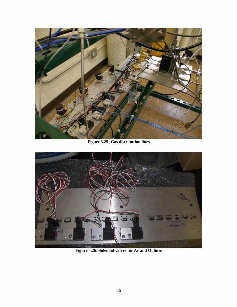
86
Figure 3.25: Gas distribution lines
Figure 3.26: Solenoid valves for Ar and O2 lines

87
3.5.5 Solenoid Valve Power Supply Box
A combination power supply and switch box was designed so that all of the solenoid valves
could be controlled easily from a central location on the system rack. The final labeled switch
box can be seen in Figure 3.3. Figures 3.27–3.29 show the main parts of the power supply at
various stages of completion. Figure 3.27 shows the inside ―base‖ of the power supply which
consists of two variable voltage 1.2 A DC power supplies (which both require wall power) and a
wall line (which is approximately 120 V at 15 A). As can be seen in the picture, two of the
connectors (on each DC supply) had to be ―jumpered‖ together (by soldering them to a piece of
wire) so as to set the output voltage to 24 V DC. These power supplies are used to operate the
solenoid valves connected to the pneumatic valves that control the MFCs, the QCM shutter, and
the magnetron gun shutters. The four solenoid valves powered by the wall line are used to
operate the pneumatic valves attached to the working and reactive gas injection lines. These
valves are shown in Figure 3.26 (being attach to the plate which holds the solenoid valves).
The metal L-bracket to the right side of the power supplies is the master ground for all the three
wall lines used in the box. The blue ―caps‖ shown are called wire nets and are used to connect
multiple wires together so that they may be easily disconnected at a later date if necessary.
(Although they may be difficult to see, there are also air holes in the sides of the supply with
protective grills on the exterior of the box, as well as rubber feet on the bottom of the supply box
to prevent it from moving.) The four (of seven) grey connectors shown are all female (electrical)
quick connects. Quick connects are used so that the electrical connections may be disconnected
and the top and bottom halves of the power supply separated for easy maintenance.
Figure 3.28 shows the exterior of front and top of the power supply box. This was an early
picture as only the switches and 115 V light bulbs are installed. Figure 3.29 shows the interior of
the power supply top halfway through completion. Note the male quick connects and more blue
wire nets that were used to connect up to 6 wires in parallel. The back of the power is located
near the front of the picture; the female plugs shown are soldered to the wires in the box and then
sealed with (heat) shrink tubing to ensure a secure connection and eliminate any chance of
electrical shorts. The metal clips on the side of the plugs rotate so that when the male plugs,
which are connected to the solenoid valves, are plugged into the back of the box they may be

88
locked in place. (As a safety note, the power should always be disconnected from the wall when
working on the interior of the power supply box even though the connections are sealed.) Not
shown are the light emitting diodes (LEDs) and voltage regulators used to create the indicator
lights for the 24 V solenoid valves.
The indicator lights had to be connected to their corresponding solenoid valves in parallel but
after the on/off switch so as to properly indicate supply of current to the valve without decreasing
the current available. The circuit diagrams for the completed power supply circuits are shown in
Figures 3.30 and 3.31. These diagrams are for the DC circuits and AC circuits, respectively.
(Note that there are 2 sets of DC circuits, Figure 3.30 applies to both as they are identical.) Note
that no ground is shown in Figure 3.30 as the lower voltage solenoid valves did not require the
use of a separate grounding wire (as long as their 24 V DC supply was grounded). The four 115
V valves from Figure 3.31 all required separate ground lines that were then connected together
and linked to the primary ground in Figure 3.27. Also note that each connection point is
indicated in these circuit diagrams, this makes the schematic more complicated than a simple
electrical diagram, but it will prove considerably more useful if and when repairs become
necessary for the power supply.
Figure 3.27: Two DC supplies and three wall line inputs inside of the power supply
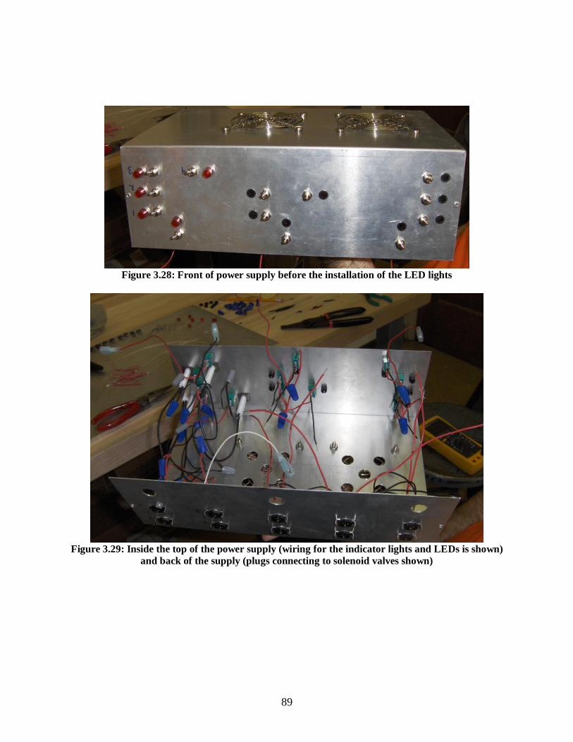
89
Figure 3.28: Front of power supply before the installation of the LED lights
Figure 3.29: Inside the top of the power supply (wiring for the indicator lights and LEDs is shown)
and back of the supply (plugs connecting to solenoid valves shown)

90
Fig
ure
3.3
0:
DC
cir
cuit
in
sid
e so
len
oid
po
wer
su
pp
ly

91
Fig
ure
3.3
1:
AC
cir
cuit
in
so
len
oid
pow
er s
up
ply

92
3.6 Safety and Support Systems
In addition to the Magnetron sputtering and Gas Distribution subsystems, there are many
auxiliary systems required to allow these components to function normally. These systems
include basics such as an adequate coolant supply as well as the foundation for more advanced
safety-related features.
3.6.1 Coolant Supply
Several components in the system require active cooling in order to maintain operability. The
magnetron sputtering system, main turbopump (TMP 351) and the sample stage (heater) all have
a range of coolant flow rates and pressures to be met. The main wall line (or primary lab water
supply) has been determined to meet the minimum pressure for all required subsystems. There is
a primary release (or shut-off valve) connected to the insulated main water line. This line then
connects to the water manifold which consists of three smaller secondary lines, each with a shut-
off (or release) valve. Finally these three lines each have two smaller variable open valves
attached to them. Each subsystem is connected to one of the tertiary releases on the water
manifold (and any extra valves are currently blanked off until they are required). The variable
open valves allow for control of the flow rate through the water lines.
The coolant (water) is transported across the room in either ½ in. or ¾ in. O.D. flexible plastic
tubing. The lines are routed along the periphery of the lab, behind the workbench, and are
protected by large interlocking rubber mats (that have channels underneath them for the lines) to
allow for the replacement of components, such as the gas supply, without fear of damaging the
coolant lines. The lines are connected to the system using corrosion resistant all plastic push
connects (that can also be used with air). The push connects allow for simple and quick draining
of water lines and maintenance activities when necessary. The quick connects also work as
reducers so that the water lines may be connected to flow meters and to the internal tubing of the
subsystems. (The magnetron guns and sample stage all use ¼ in. O.D. tubing.) After passing
through the subsystems, the water lines are routed back along the same path to a common drain.
(It would be possible to instead use a large independent cooling system so as to constantly re-
circulate the coolant water but these were cost prohibitive and would only be required for larger
coolant flows or situations where the system is constantly operating.)

93
Each magnetron gun requires 1 to 2 gallons per minute (gpm) at a pressure of 30 to 60 psi in
order to keep the magnets cooled. (The coolant required also depends on the target voltage, but
the range stated here is adequate for all operating power levels that the power supplies are
capable of producing.) Without proper cooling the magnets will ―wear out‖ or, more accurately,
being exposed to high temperatures will allow the atomic structure of the magnets to rearrange
thus weakening and eventually eliminating the magnetic field produced by the magnet.
Similarly, the turbopump may also be damaged by exposure to high temperatures. However, it
has a safety shut-off that will trip the pump (turning it off) in case the temperature becomes too
high. Its coolant flow requirements are minimal at 0.1 to 0.2 gpm. Finally, the sample stage will
also require cooling when the substrate heater is in use. The sample stage needs approximately 1
gpm but is sensitive to high flow rates which may induce vibration in the sample stage. It does
not have an automatic shut-off and is thus one of the primary safety concerns for the system.
Without adequate cooling, the substrate heater (and sample stage) could cause the entire system
to overheat thus damaging seals and any equipment directly contacting the system that is
sensitive to temperature. Therefore, additional measures have been taken to ensure adequate
coolant is supplied and that gas pressure remains suitably low to prevent this occurrence. (A high
gas pressure would allow for convection to occur so that heat is transferred to the surrounding
chamber by a means other than radiation and conduction. This would cause the rest of the
chamber, which only has a maximum temperature of 150°C as opposed to 850°C, to heat up very
rapidly.)
3.6.2 Interlocks
Safety interlocks are used to monitor operating parameters relevant to the safe operation of the
system. ―When a parameter falls outside of the parameter ‗window‘ a specific action is initiated‖
by the interlock [2]. The sputtering system currently employs an interlock that measures both the
coolant flow rate through the sample stage (by means of a waterwheel) and gas pressure within
the main chamber (via one of the pressure sensors), this interlock then trips the power supply to
the substrate heater if the pre-set values are not met. Tripping the power supply will turn off the
heater or not allow it to be turned on again if it is already off. (Both the pressure trip point and

94
water flow trip point must be set manually. The flow rate trip point is always active but the
pressure trip point may be de-activated with the flip of a switch. It is currently deactivated.)
Even with interlocks it should be noted that the current safety-related feature set necessitates
operators be on hand at all times during film growth and while pumping down on the system.
The system has not yet been fully-automated in terms of shutdown scenarios. For example, pump
coolant must be turned on manually and there is no interlock for the case of a loss of coolant
accident (LOCA). (Although this is a very unlikely accident scenario as it would be caused by a
loss of water throughout the entire building or a breach in the water lines.) A LOCA would cause
the turbopump to shut down. This would in turn cause the roughing pump to pump on the main
chamber which could cause back streaming (of pump oil into the chamber). ―If oil migrates into
the deposition chamber it can contaminate the substrate surface before film deposition or be
decomposed in a plasma to deposit contaminants such as carbon‖ [2]. To remedy this potential
scenario an interlock and flow meter combination could be used, like in the case of the substrate
heater, to either shut the GV or to turn off the roughing pump.
A similar accident scenario may also be caused by loss of power to the turbopump or roughing
pump. Back-up power supplies could be used with interlocks to initiate a shut-down of the
system, but this is a considerably costly remedy. A simpler solution would be to install a
normally closed (NC) wall-powered solenoid valve between the turbopump and the roughing
line. When the power is lost the valve automatically closed. (Currently there is a manual valve
here so that the same action may be performed manually by the operator.) However, this may
still cause back-streaming into the roughing line. To prevent this (and maintain the highest
system purity) a normally open (NO) solenoid ―leak valve‖ connected to the Argon gas supply
could be used such that a constant pressure of Argon flows through the line, then through the
roughing pump and out the exhaust line so as prevent back streaming. (Again, there is already a
manual valve located here so this action can currently be performed by an operator if present.)
As the load-lock pump is also connected to the same roughing pump as the main pump, it should
also have a NC valve. (It too currently has a manual valve.) Finally, in the case of short power
outage where the operator is not on hand to de-activate all equipment, a vacuum pressure switch
can be added to the (NC) roughing valves so that they would not reopen until the Argon gas in

95
the roughing lines had been pumped down to a sufficiently low pressure. (This step is also
currently performed manually by the operator by using a thermocouple pressure gauge to
measure the roughing line pressure.)
Finally, there are safeguards for user error. The pressure interlock has already been mentioned
for the substrate heater (which is by far the worst potential accident scenario). Still several other
systems, such as the ion gauges and magnetron guns, should not be operated at high pressures.
(Certain systems like the ion gauges automatically de-activate at high pressures.) The simplest
solution is to prevent the system from reaching high pressures; this is detailed in the next
subsection. However, if added security is later requested, the aforementioned ―vacuum switches
can be used to prevent … high voltage from being applied when the system is not under
vacuum‖ [2].
3.6.3 Pressure Relief Valves
Additional safeguards have been put in place to prevent an over-pressurized environment (i.e.
greater than atmospheric pressure) from developing as many of the vacuum monitoring
components may be damaged or need to be recalibrated as a result. (Components like the
Baratron were designed so that at 45 psia ―the diaphragm will bottom out on the electrode
substrate, preventing permanent damage to the sensor‖ and only requiring it to be calibrated
[15].) To prevent this accident scenario, two adjustable cracking pressure check valves can be
used as ―relief valves‖ by setting the ―cracking pressure‖ (or pressure at which the valves opens
and allows gas to flow out) to a pressure near atmospheric pressure. (Note that these valves are
not certified as code safety relief devices.) The valves are both ¼ in. Male VCR valves which are
certified as cleaned (by the manufacturer) and packaged in Argon gas. The valves provide for
directional gas flow and the cracking pressure may be manually adjusted from 3 to 50 psi.
As there are two valves, one may be connected to the main chamber (possibly to the extra VCR
port on the top flange via use of an adapter) and one to the load-lock chamber. However, it is
also possible to vent the load-lock using the load lock door (by not tightening the ―swing-away
hand knob locking mechanism‖ shut thus allowing it to open automatically once the pressure is
greater than atmospheric pressure) so the relief valve may be unnecessary for this particular
system. It is also possible to vent the main chamber through the load-lock. (Nevertheless there is

96
the remote possibility of an accident scenario in which the manual-GV and the automatic GV are
forced shut with gas flowing into the main chamber, in which case a tertiary form of pressure
relief would be necessary.)
3.7 Maintenance and Cleaning
Regular maintenance and cleaning will need to be performed on the magnetron sputtering
system. For practical and convenience purposes, it was designed to minimize down times
associated with these tasks.
3.7.1 Maintenance
The filters for the ―oil traps‖ in the roughing pumps will need to be replaced once every three
months (or less often if the system is only used irregularly). The exact replacement schedule for
the QCM crystals has not yet been determined because full-time regular operations have not yet
commenced. After a significant amount of material has been deposited on one of the crystal the
shutter will be switched to reveal the second fresh crystal. To minimize down time they will
replaced simultaneously most likely after several months of operation.
The sputter targets will need to be replaced once significant erosion has occurred. (The depleted
Uranium target will be disposed of in accordance with all safety requirements.) Finally, the light
bulbs for the substrate heater will also need to be replaced on occasion. The QCM crystals, light
bulbs, targets, oil trap filters, and gas tanks should be the extent of parts that need regular
maintenance and/or replacement. All cleaning and maintenance operations (internal to the main
chamber) will require the safe shut down and start-up of the system (after being baked out after
cleaning.) These procedures have been written and supplied by Professor Heuser and are
provided in Appendix B as supplementary material.
3.7.2 Cleaning and Liners
In order to perform cleaning and maintenance the system will need to be returned to the ambient
pressure by venting or backfilling the chamber with air (or an inert gas). ―If this venting takes
place rapidly, particles can be stirred-up in the system‖ [2]. Given the fact that the system is
coated in uranium (and other heavy metals), this effect should be avoided by allowing the
pressure to rise slowly. Additionally, whenever the system is opened for maintenance functions,

97
the main chamber will be vacuumed to remove all the debris or particulates that have
accumulated due to sputtering. A metal vacuum with a HEPA filter will be used in order to
prevent contamination by the uranium ―dust‖ and minimize exposure. This material will then be
disposed of in accordance with all university and governmental regulations.
During cleaning, rubber gloves will be used at all times. The components may be blown clean by
use of the gas gun and any available inert gas (such as Argon). (This is to remove particulates
from fixturing only; the contaminants will not be blown out of the system but rather to a location
where they may more readily be vacuumed. Face masks with air filters would be worn while
performing this action.) While cleaning care must be taken not to damage (i.e. scratch) any of the
surfaces or to increase the surface area by any other means. Cleaning may include the viewport
window as necessary (to increase visibility if it becomes a concern). The cleaning of metal
surfaces will typically involve a de-ionized water (DI) rinse and the use of a solvent. Acetone is a
commonly used solvent, but it leaves a residue that must be cleaned with an alcohol such as
ethanol or isopropyl alcohol (IPA). All components/surfaces cleaned will receive a final wipe
down with KimWipes and methanol so as to remove particulates and water vapor, respectively.
At this time liners (or shields) are not used within the chamber. ―Liners and shields are used to
prevent deposition on non-removable vacuum surfaces,‖ and can be disposable or reusable (and
cleanable) [2]. Liners were investigated, but ultimately rejected as they would increase the
surface area in the chamber and may restrict gas conductance into the pumping stack (and out of
the chamber.) This is because the internal geometry of the chamber and space constraints
dictated where the liners could be installed and the locations were not optimal. Still, there is
some evidence that it might be beneficial to place a thin disposable liner at the bottom of the
chamber (near the base of the magnetron guns). This would make it easier to dispose of the
particulates produced in the system via sputtering. This liner could be as simple as a piece of
aluminum foil (clean, non-oiled).
After the scheduled cleaning (and maintenance) has been completed, the system will be restarted
in accordance with the procedures shown in Appendix B. After which the system will be baked
out for several days to remove any contaminant gases introduced by exposure to the ambient. In

98
order to reduce the time required for baking out, a slightly positive pressure gradient of Argon
gas (i.e. a pressure greater than atmospheric pressure) may be used during cleaning (although the
gas flow will be minimal so as not to waste Argon and to alleviate safety concerns related to
inhalation). This is done to reduce the amount of water vapor that enters the chamber while it is
open. The pressure can be verified using the 1000 Torr Baratron and the adjustable cracking
valves (before the chamber is opened). Additionally, sometimes dry gas is flowed through the
chamber during the bake-out procedure to help remove released gases.
3.8 Sample Storage
Although not technically part of the system, there are several storage options available for
completed film samples. The storage methods are designed to mitigate the post-deposition
contamination of the films. Examples of post-deposition include oxidation of the completed film
or the adsorption of contaminants such as hydrocarbons. (Water vapor accumulation can also be
detrimental to films.) While inside the system, post-deposition contamination will remain
unlikely.
Unfortunately, at some point in the transfer (for analysis) and/or storage process the film samples
will need to be exposed to the ambient (i.e. the external) environment. This time will be kept to a
minimum. When transported the films will usually be wrapped in a Kimwipe (for cushioning)
and stored in a small plastic sample case. For situations in which the utmost level of purity is
required, the lab has also recently acquired the ability to transport samples in a self-contained
vacuum system (that can be actively pumped down). (It should also be noted, that many of the
characterization techniques will be performed under vacuum in clean systems, further reducing
the odds of sample contamination.)
For the general storage of film samples, the individual plastic containers will be placed inside a
glass vacuum jar that will then be pumped down to a rough vacuum. The inside of the jar will
also contain a tray of desiccants (such as DRIERITE) to remove any excess water vapor that may
still be in the jar.
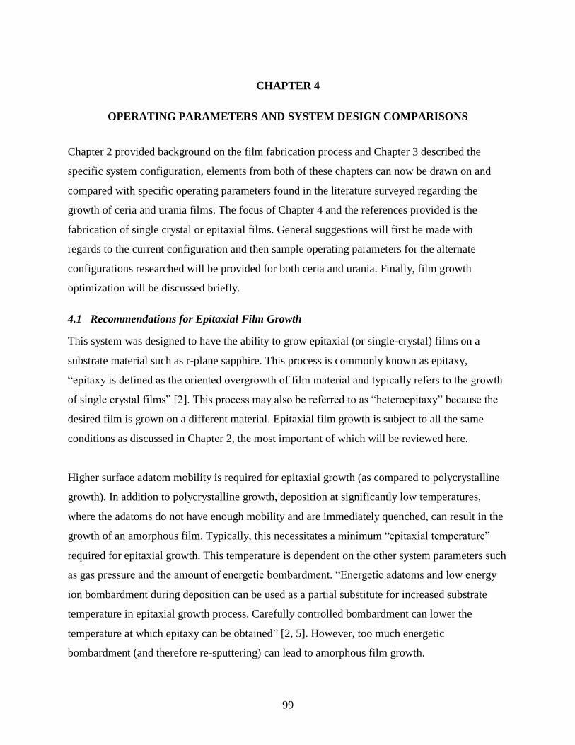
99
CHAPTER 4
OPERATING PARAMETERS AND SYSTEM DESIGN COMPARISONS
Chapter 2 provided background on the film fabrication process and Chapter 3 described the
specific system configuration, elements from both of these chapters can now be drawn on and
compared with specific operating parameters found in the literature surveyed regarding the
growth of ceria and urania films. The focus of Chapter 4 and the references provided is the
fabrication of single crystal or epitaxial films. General suggestions will first be made with
regards to the current configuration and then sample operating parameters for the alternate
configurations researched will be provided for both ceria and urania. Finally, film growth
optimization will be discussed briefly.
4.1 Recommendations for Epitaxial Film Growth
This system was designed to have the ability to grow epitaxial (or single-crystal) films on a
substrate material such as r-plane sapphire. This process is commonly known as epitaxy,
―epitaxy is defined as the oriented overgrowth of film material and typically refers to the growth
of single crystal films‖ [2]. This process may also be referred to as ―heteroepitaxy‖ because the
desired film is grown on a different material. Epitaxial film growth is subject to all the same
conditions as discussed in Chapter 2, the most important of which will be reviewed here.
Higher surface adatom mobility is required for epitaxial growth (as compared to polycrystalline
growth). In addition to polycrystalline growth, deposition at significantly low temperatures,
where the adatoms do not have enough mobility and are immediately quenched, can result in the
growth of an amorphous film. Typically, this necessitates a minimum ―epitaxial temperature‖
required for epitaxial growth. This temperature is dependent on the other system parameters such
as gas pressure and the amount of energetic bombardment. ―Energetic adatoms and low energy
ion bombardment during deposition can be used as a partial substitute for increased substrate
temperature in epitaxial growth process. Carefully controlled bombardment can lower the
temperature at which epitaxy can be obtained‖ [2, 5]. However, too much energetic
bombardment (and therefore re-sputtering) can lead to amorphous film growth.

100
It is recommended that the substrate heater be used to heat the sample holder and substrate to its
highest operational temperature of 850°C. Sample rotation should be used at all times to promote
uniform film growth. It is also recommended that films be grown with a negative voltage bias
applied to the substrate (via the sample holder) so as to minimize negative ion bombardment and
better control energetic bombardment in general (as discussed in Chapter 2.) Furthermore, the
working gas pressure should be kept as low as possible to increase both the initial energy of the
adatoms and the energy of the bombarding particles. This will also provide a more uniform
energy distribution in the particles impacting the substrate surface. (Based on information to be
presented in Chapter 6, realistically the lowest pressure attainable for the current configuration
would be 3–4 mTorr at a total flow rate of 10 sccm.) Given that the Argon MFC is a 100 sccm
unit, it is not recommended that the Argon flow rate be lowered past 5 sccm so as to ensure
reliable measurements.
Additional considerations include:
Determining the minimum partial pressure of O2 needed for stoichiometric film growth as
any additional O2 will further decrease surface adatom mobility. (This will also depend
on the system geometry, i.e. where the Argon and O2 are introduced in the system.)
Determining the maximum distance at which the substrate may be held from the sputter
source (so as to decrease the angle of incidence) before thermalization. (Alternatively,
lowering the sample holder height but adding a collimator in between the substrate and
the sputter target will have the same effect.)
Determining a sufficiently low deposition rate for epitaxial growth (that also accounts for
the reduction in rate due to re-sputtering). This allows defects to be corrected for (or
filled in) by surface diffusion before they are buried over (or ―frozen‖ into the film) by
newly deposited material
Annealing of the substrate (in addition to the preparations required to cure the silver
thermal paste) so as to remove any residual stresses that may have been present in the
substrate (possibly due to polishing). This will potentially lower the overall stress of a
film once it has been grown on the substrate.
The addition of a cold trap for the purposes of removing residual gases from the plasma
environment. (Contaminants also negatively impact surface adatom mobility.)

101
Finally, the ―oriented growth‖ of a film at low deposition temperature ―can be enhanced by ‗seeding‘ of
the substrate surface with oriented nuclei‖ [2]. This process is performed by depositing a very small
amount of the desired compound and then by annealing the substrate so as to ―form isolated orientated
grains‖ which would then acts as ―seeds,‖ or nucleation sites, for subsequently deposited film material. As
will be shown shortly, this and many of the other suggestions are all common techniques.
The above recommendations are pertinent to growth of any single-crystal film, particularly
compound films grown via reactive sputtering. Specific growing conditions (i.e. the operating
parameters) for the growth of ceria and urania films will now be discussed.
4.2 Sample Operating Parameters and Configurations for CeO2 Growth
Ceria was initially used as a surrogate for urania in the production of films at the UIUC MRL.
Knowledge gained during the production of those films will be applied to the production of films
in the sputtering system. Similarly, knowledge of other sputtering systems may also facilitate the
determination of ideal operating parameters for ceria growth. The literature discussed herein
presents various system design and their corresponding viewpoints in terms of suggested
operating parameters (some of which are competing) for epitaxial ceria growth.
The most similar set-up [7] uses r-plane sapphire substrates and DC sputtering at temperatures
ranging from 600°C to 850°C. The total pressure was at 7.5 mTorr with an Argon-Oxygen ration
of 3:1 (or 75% and 25%, respectively). The substrate to target distance was fixed at 5 cm. The
results of the analysis [7] were that the higher the substrate temperature, the closer to epitaxial
the films became. However, they were unable to produce epitaxial ceria films on r-plane sapphire
due to the elastic strain caused by the lattice mismatch. (There were always some (111) crystals
mixed in with the (200) orientation, although this decreased as temperature increased and the
stress was alleviated.) It is important to note that this does not necessarily mean it will similarly
prove impossible to produce epitaxial films in the designed system as the deposition rate was
exceedingly high; however, it would suggest that using elevated temperature and DC sputtering
may not prove to be the best way to achieve the production of single-crystal films.

102
Several other papers in the literature relied on the system configuration shown in Figure 4.1. [20,
21, 19] This system is a significant departure from the design system in that it relies on an
Oxygen radical source and also uses an RF plasma in conjunction with a DC plasma. (The
literature also stated that seed layers were used in the production of the films.) Nevertheless, the
points brought up in the literature are still indicative of processes discussed in Chapter 2 and the
resulting effects that may be encountered.
Figure 4.1: Sample magnetron sputtering diagram with oxygen radical source [19]
As discussed in Chapter 2, the substrate temperature has an important role in film quality. The
literature used in Chapter 2 and Chapter 4 both indicate that most films have a minimum
epitaxial temperature below which epitaxial growth cannot be achieved. The literature also states
that this temperature may be affected by numerous other operating parameters.
Work performed [19] proves that increasing the reactivity of the (reactive) species will lower the
epitaxial temperature, or for the same temperature, produce a higher quality film. As noted
earlier, this is because ―activation of the reactive species enhances chemical reactions during
reactive deposition‖ [2]. There are two factors involved in increasing the reactivity of the system

103
[19] used: the first is the radical source, the second is that it is ―enhanced with an inductively
coupled RF plasma‖ [2]. The RF plasma can be used to produce a denser and more uniform
plasma near the target and to increase the size of the plasma volume overall. This also increases
gas reactivity because ―the plasma used in sputtering will activate the reactive gases‖ [2].
However, it should be noted that a secondary plasma may instead be generated in between the
substrate and the target. Figure 4.2 shows an inductively coupled plasma. This plasma may be
used to produce ―post-vaporization ionization.‖
―Ionization values as high as 70% have been reported using an rf-excited plasma.‖ ―These film
ions can be accelerated to the substrate surface by applying a potential to the surface. This tends
to give a more-normal direction to the depositing flux.‖ [2]
Figure 4.2: Inductively coupled RF plasma (ICP) source
(Note: coil does not have to be external to the chamber; this is only one type of ICP source) [2]
Alternatively, ―auxiliary electron sources can be used to enhance the plasma density between the
target and the substrate.‖ Electrons may also be ―used to heat surfaces and to ionize atoms and
molecules.‖ ―Ionization can be enhanced by having an flux of energetic (100 eV) electrons
between the target and the substrate.‖ The most common source of electrons is a hot electron
(thermoelectron) emitting surface‖ (e.g. a tungsten or thoriated tungsten filament). [2]
It is important to note that the secondary plasma should not extend all the way to the substrate
surface or the resulting resputtering will actually negatively impact film quality [22]. One
reference [22] goes so far as to say that ―the resputtering effect should be avoided if high-quality

104
CeO2 films are to be obtained by reactive sputtering‖ but this reference only accounts for
resputtering due to ―negative ions from the target‖ that are accelerated toward the substrate. It
does not mention the effects of neutral bombardment nor explain that negative ion bombardment
can be countered with a voltage bias and that preferential bombardment can be favorable as do
the other references used in this thesis. However, it was similar in that it was operated with an
RF plasma at a pressure less than 1 mTorr, at elevated temperature and low deposition rate with
the substrate close enough to the sputter target to ensure high energy transfer even at an oblique
angle. [2, 20, 21, 19, 22]
An additional benefit to ionizing the gas species (and the metal atoms) besides increasing
reactivity and decreasing the angle-of-incidence is that it also increases the energy of the
impinging particles and can cause preferential crystal orientation. [21,19] A reference [21]
concluded that a bias of -15 V was most ideal for their given system at a temperature of 850°C, a
Ar-O2 ratio of 6:1, and an operating pressure of approximately 1 mTorr. (Again, the use of the
RF plasma allowed for a lower operating pressure and thus higher energetic bombardment.)
Furthermore the same set-up and similar conditions were used to show that ―orientation
selectivity is found to be dependent not only on substrate bias but on the growth rate‖ as well
[21]. As the deposition rate was increased (by increasing the Argon gas flow rate and thus sputter
target bombardment) the possibility of (100) formation increased ―due to increase in the kinetic
energy of adsorbed atoms and/or molecules for their migration needed for occupancy of epitaxial
sites‖ [21]. (Again, the pressure was held at a pressure below 1 mTorr.)
Finally, to provide an opposite viewpoint, Reference [9] proves it is possible to produce an
epitaxial film at high pressures given an elevated temperature and low deposition rate (and other
factors). Epitaxial films were grown at 110 mTorr with an RF power supply set to approximately
100 W at a deposition rate of 0.5 Angstroms per second. The temperature was approximately
810°C and the sample was off-axis (most likely to reduce resputtering). However, in order to
produce the epitaxial film, the process required post-deposition annealing in an oxygen
environment [9]. Therefore, even if perfect single crystal films were unable to be produced in
designed at UIUC, this would suggest that it still may be possible to take the films and perform
post-processing to achieve the originally desired film quality.
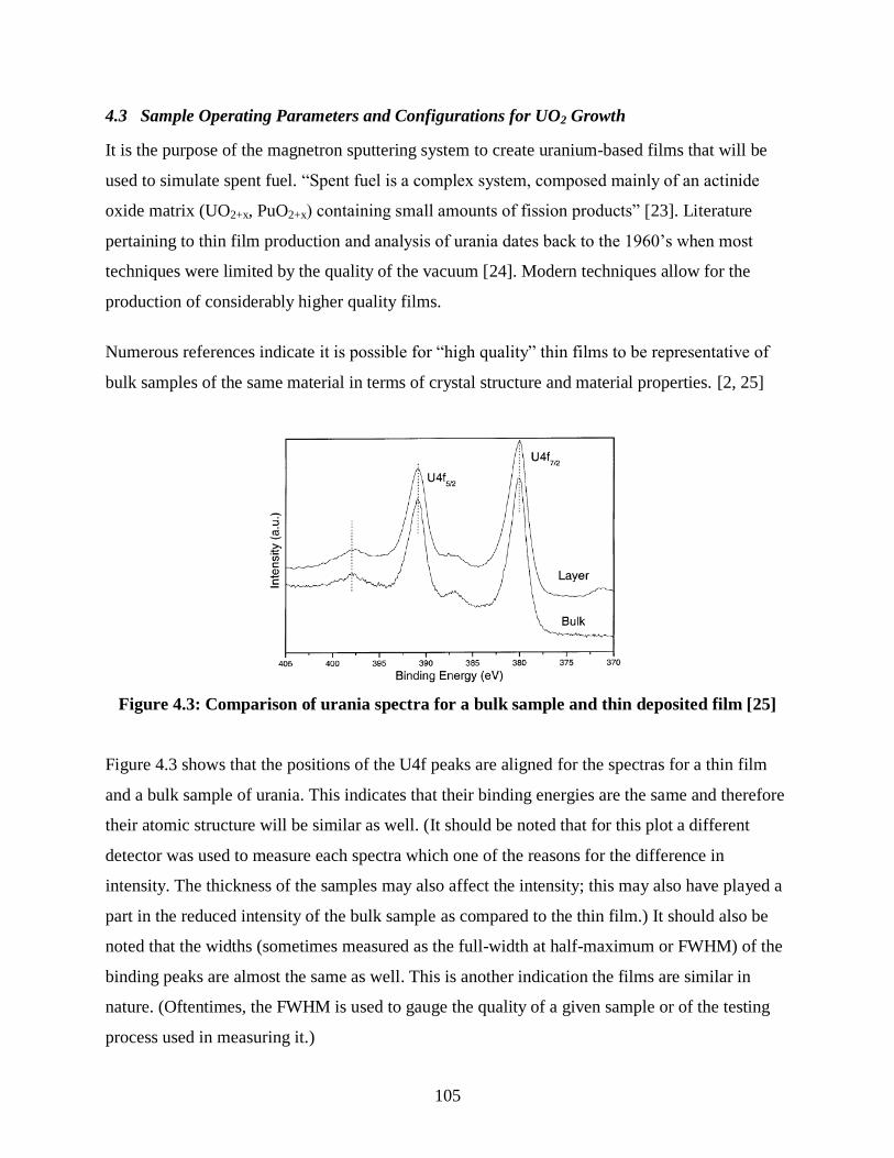
105
4.3 Sample Operating Parameters and Configurations for UO2 Growth
It is the purpose of the magnetron sputtering system to create uranium-based films that will be
used to simulate spent fuel. ―Spent fuel is a complex system, composed mainly of an actinide
oxide matrix (UO2+x, PuO2+x) containing small amounts of fission products‖ [23]. Literature
pertaining to thin film production and analysis of urania dates back to the 1960‘s when most
techniques were limited by the quality of the vacuum [24]. Modern techniques allow for the
production of considerably higher quality films.
Numerous references indicate it is possible for ―high quality‖ thin films to be representative of
bulk samples of the same material in terms of crystal structure and material properties. [2, 25]
Figure 4.3: Comparison of urania spectra for a bulk sample and thin deposited film [25]
Figure 4.3 shows that the positions of the U4f peaks are aligned for the spectras for a thin film
and a bulk sample of urania. This indicates that their binding energies are the same and therefore
their atomic structure will be similar as well. (It should be noted that for this plot a different
detector was used to measure each spectra which one of the reasons for the difference in
intensity. The thickness of the samples may also affect the intensity; this may also have played a
part in the reduced intensity of the bulk sample as compared to the thin film.) It should also be
noted that the widths (sometimes measured as the full-width at half-maximum or FWHM) of the
binding peaks are almost the same as well. This is another indication the films are similar in
nature. (Oftentimes, the FWHM is used to gauge the quality of a given sample or of the testing
process used in measuring it.)

106
Uranium can be used to form several different complex compounds because it ―exists in
oxidation states +2 (gas phase), +3, +4, +5, and +6 in the solid state and in solution‖ [26]. (The
type of compound determines the binding energy of the valence electrons.) Uranium oxides
―exist in different compositions (UO2, U4O9, U3O8, UO3)‖ [23]. However, the system will
primarily be used to grow urania (UO2) or variations thereof (UO2+x or UO2-x). Urania is not
commonly encountered in nature, yet it is far easier to produce than forms that require higher
oxidation (UO3, etc.). In fact, ―it is unlikely that deposition at‖ substrate temperatures higher than
573K ―would yield higher oxidation states, because the temperature of the plasma during the
deposition is much higher than that of the substrate, and increased substrate temperature results
in low oxygen sticking probability‖ [26, 23].
As a rule, ―the transformation of UO2 to UO2+x is slower compared to the oxidation of U metal to
UO2.‖ ―One possibility to produce higher oxides is to create strong local oxidation conditions on
the substrate surface compared to the target, e.g. by adding an oxidation catalyst (Cs) to the film‖
[23]. On the other hand, production of substoichiometric urania (UO2-x) will be relatively easy. It
will simply require the use of dopants such as cerium or lanthanum to replace uranium in the
crystal lattice. These can be co-sputtered or can be introduced as a vapor (e.g. Cesium from a
heated filament). These dopants will effectively be the actinide surrogates in the urania film so
that it may better approximate ―spent fuel.‖ The system is currently set-up to use Cerium and
Neodymium sputter targets for co-sputtering. (There are currently no plans for a heated element
source to be added.)
As was the case for the literature on producing ceria samples, it is difficult to find information
directly pertaining to fabrication parameters available to the system in its current configuration.
Studies [23] and [25] are similar in that they both used DC sputtering; however, they also relied
on the addition of electrons to maintain the plasma and/or for ionization. The fact that additional
electrons were required would suggest that the system was maintained at a low pressure and a
relatively low deposition rate (for the reasons discussed in Chapter 2). The set-up in [25] used a
low pressure of 3 mTorr and a large voltage bias of -500 V. (It should be noted that films grown
in [25] were grown on Silicon substrates, not sapphire.) Films grown via the set-up in [23] did
not use voltage biasing but were grown at elevated temperature.

107
Although the exact pressures and other parameters varied between these set-ups, they both
agreed on the importance of controlling and minimizing the partial pressure of Oxygen ―because
at a critical threshold‖ of O2 partial pressure of approximately 0.75 mTorr ―the target itself
oxidizes‖ which ―results in the formation of an insulating or semiconducting oxide overlayer
which disrupts the DC plasma‖ [23]. Or, in other words, ―at .375mTorr partial pressure O2 it
becomes ―difficult to ignite the plasma‖ as the ―metallic uranium oxidizes too fast‖ thus
hindering ―the formation of the DC electric field that is required to form the plasma‖ [25].
However, the minimum partial pressure required to form stoichiometric urania is quite low. ―At
.075 mTorr O2 partial pressure spectra remains stationary and matches that of bulk‖ [25]. This is
also confirmed in Figure 4.4 where it shows that only .075 mTorr (or 0.0001 mbar) is required to
obtain the proper spectra (or U4f binding energies) such that it matches those in Figure 4.3.
(Note that the geometry of the reactive gas injection, as well as the reactivity of the oxygen gas
will also affect the partial pressure required. The system shall most likely need a greater partial
pressure for stoichiometric films but if optimized properly it should not be significantly greater.)
Figure 4.4: Comparison of U-4f peaks for various UOx films with varying O2 partial pressure
(Note: 1 mbar = 0.75 Torr or 750 mTorr) [23]

108
4.4 Film Growth Rate Optimization
Using ―the commonly accepted treatment‖ known as ‗Berg‘s Model‘ to compare several
different operating parameters with respect to sputtering rate, the system behavior can be better
understood and preliminary work on film growth rate optimization can begin [6]. The most
obvious example where this is applicable pertains to reactive gas availability as shown in Figure
4.5.
4.4.1 Sputter Erosion Rate, Reactive Gas Pressure, and Flow Rate
Figure 4.5: Plots provide information on the Optical emission (OES) peak height which indicates
the sputter rate (Left) and Pressure (Right) as functions of reactive gas flow
As noted in the gas availability subsection, while ―forming a compound of the deposited film,
compound formation will also take place at the surface of the sputtering target‖ and ―normally,
the sputtering yield of the compound material is substantially lower than‖ for the ―target
material.‖ [6, 2] (Although these yields can be affected by other factors, they are generally
considered material constants.) This is the reason why increasing the supply of the reactive gas
unnecessarily will decrease the sputter rate (or target erosion rate) and therefore deposition rate
of the film.
Figure 4.5 shows that there is an additional feature (typically) inherent to this process. Both the
―sputter erosion rate vs. the supply of the reactive gas for a reactive sputtering process (carried
out with constant target current during processing)‖ (left) and ―the relationship between the
partial pressure and the supply rate of reactive gas‖ (right) ―exhibit a hysteresis effect‖ [6]. (Note
that the hysteresis will be less pronounced if the sputter yield of the compound is similar to that
of the target.) ―The hysteresis effect is one of the key problems encountered in experimental

109
reactive sputtering system‖ although the hysteresis does not always occur, depending on the
system conditions [6].
With regards to the plots shown in Figure 4.5, the presence of the hysteresis means that the
deposition rate and the partial pressure, respectively, will not increase and decrease at the same
value (with respect to pressure) but rather depend on whether the reactive gas is being increased
or decreased at the given time. Figure 4.5 (left) shows that the sputter rate is initially high as the
reactive gas supply is increased (from zero flow) until the flow reaches some point where the
sputter rate drops sharply. On the other hand, approaching the system with a high reactive gas
flow rate causes the target sputter rate to remain low until it reaches a different point at which it
increases sharply.
Similarly, Figure 4.5 shows that ―during the increase sequence of the reactive gas supply, the
partial pressure of the reactive gas remains at a very low level until reaching the upper limiting
value of the hysteresis width.‖ Conversely, ―during a decrease of the supply of the reactive gas,
the partial pressure remains significantly higher in the hysteresis region than during the increase
of the gas.‖ Taken as a whole, the information in Figure 4.5 demonstrates ―that more gas is
consumed for compound formation during the increase sequence‖ because the ―higher sputter
erosion rate needs more reactive gas to form‖ the compound material. Together, this provides a
significant part of the information required for growth rate optimization. [6, 2]
However, it is important to note that controlling a process by the supply (or flow rate) of the
reactive gas is not the same as controlling it based on the partial pressure, the system will react
differently depending on which is used. Additionally, the flow rate can be selected manually and
automatically controlled by the MFC whereas the partial pressure will vary and can only be
measured by using the mass spectrometer. ―The appropriate gas composition and flow for
reactive sputter deposition can be established by monitoring the partial pressure of the reactive
gas as a function of reactive gas flow‖ [2, 6]. This is shown if Figure 4.6 (right) for the specific
case of a TiN film grown via reactive deposition using a pure Ti target and N2 gas.
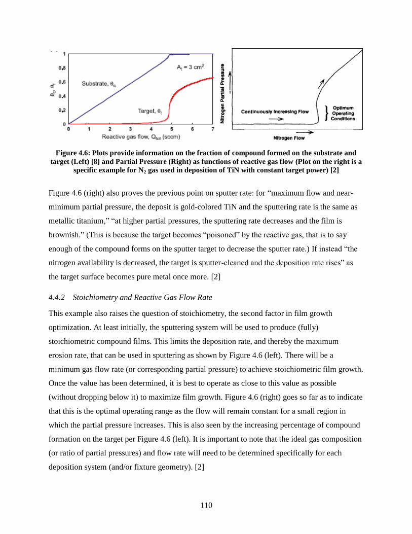
110
Figure 4.6: Plots provide information on the fraction of compound formed on the substrate and
target (Left) [8] and Partial Pressure (Right) as functions of reactive gas flow (Plot on the right is a
specific example for N2 gas used in deposition of TiN with constant target power) [2]
Figure 4.6 (right) also proves the previous point on sputter rate: for ―maximum flow and near-
minimum partial pressure, the deposit is gold-colored TiN and the sputtering rate is the same as
metallic titanium,‖ ―at higher partial pressures, the sputtering rate decreases and the film is
brownish.‖ (This is because the target becomes ―poisoned‖ by the reactive gas, that is to say
enough of the compound forms on the sputter target to decrease the sputter rate.) If instead ―the
nitrogen availability is decreased, the target is sputter-cleaned and the deposition rate rises‖ as
the target surface becomes pure metal once more. [2]
4.4.2 Stoichiometry and Reactive Gas Flow Rate
This example also raises the question of stoichiometry, the second factor in film growth
optimization. At least initially, the sputtering system will be used to produce (fully)
stoichiometric compound films. This limits the deposition rate, and thereby the maximum
erosion rate, that can be used in sputtering as shown by Figure 4.6 (left). There will be a
minimum gas flow rate (or corresponding partial pressure) to achieve stoichiometric film growth.
Once the value has been determined, it is best to operate as close to this value as possible
(without dropping below it) to maximize film growth. Figure 4.6 (right) goes so far as to indicate
that this is the optimal operating range as the flow will remain constant for a small region in
which the partial pressure increases. This is also seen by the increasing percentage of compound
formation on the target per Figure 4.6 (left). It is important to note that the ideal gas composition
(or ratio of partial pressures) and flow rate will need to be determined specifically for each
deposition system (and/or fixture geometry). [2]
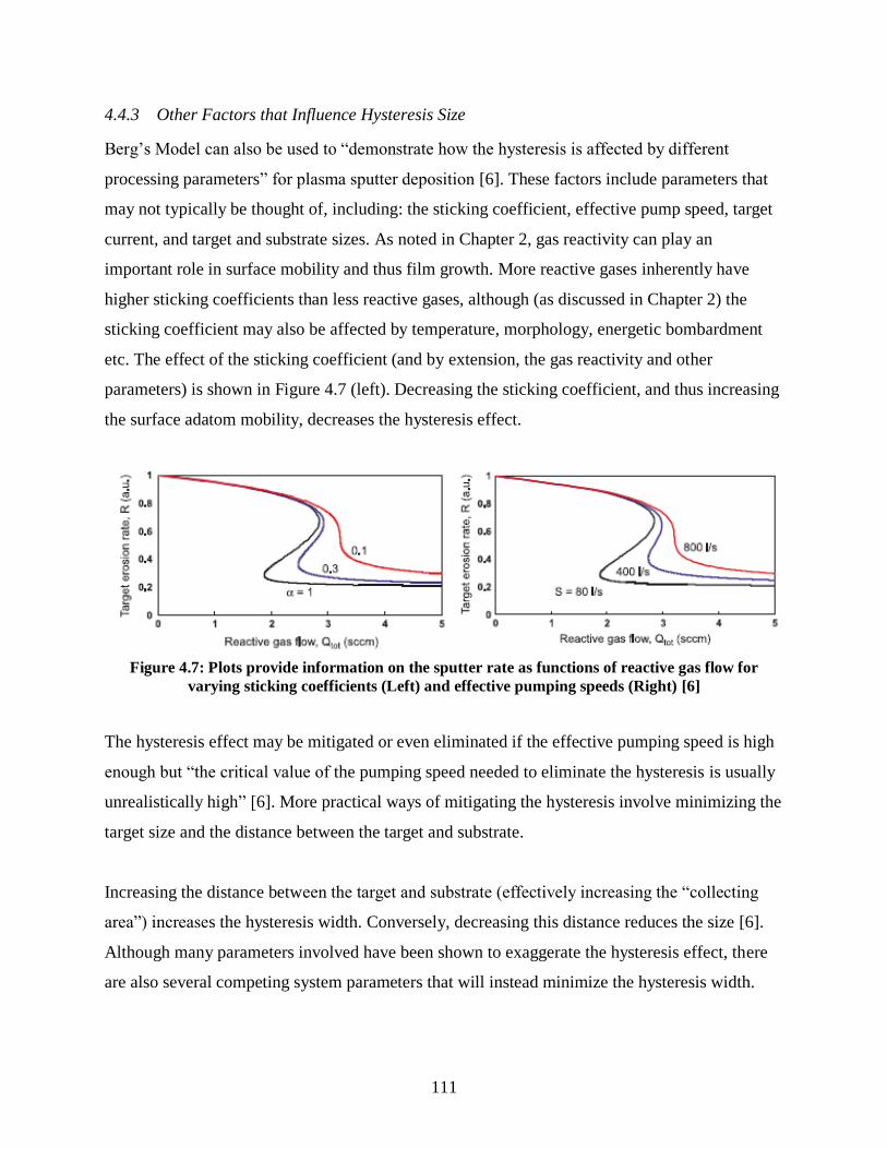
111
4.4.3 Other Factors that Influence Hysteresis Size
Berg‘s Model can also be used to ―demonstrate how the hysteresis is affected by different
processing parameters‖ for plasma sputter deposition [6]. These factors include parameters that
may not typically be thought of, including: the sticking coefficient, effective pump speed, target
current, and target and substrate sizes. As noted in Chapter 2, gas reactivity can play an
important role in surface mobility and thus film growth. More reactive gases inherently have
higher sticking coefficients than less reactive gases, although (as discussed in Chapter 2) the
sticking coefficient may also be affected by temperature, morphology, energetic bombardment
etc. The effect of the sticking coefficient (and by extension, the gas reactivity and other
parameters) is shown in Figure 4.7 (left). Decreasing the sticking coefficient, and thus increasing
the surface adatom mobility, decreases the hysteresis effect.
Figure 4.7: Plots provide information on the sputter rate as functions of reactive gas flow for
varying sticking coefficients (Left) and effective pumping speeds (Right) [6]
The hysteresis effect may be mitigated or even eliminated if the effective pumping speed is high
enough but ―the critical value of the pumping speed needed to eliminate the hysteresis is usually
unrealistically high‖ [6]. More practical ways of mitigating the hysteresis involve minimizing the
target size and the distance between the target and substrate.
Increasing the distance between the target and substrate (effectively increasing the ―collecting
area‖) increases the hysteresis width. Conversely, decreasing this distance reduces the size [6].
Although many parameters involved have been shown to exaggerate the hysteresis effect, there
are also several competing system parameters that will instead minimize the hysteresis width.

112
This system uses a 3-inch target and ―a small target exhibits almost ideal processing conditions‖
[6]. Figure 4.8 provides a relative comparison of hysteresis size based on sputter rate and target
area, At. For a 3-inch target, more reactive gas flow will be needed to reach the hysteresis region
and the hysteresis is notably smaller. ―The critical size‖ required to eliminate the hysteresis
entirely is dependent on the other system parameters and ―for the specific reactive sputtering
process‖ [6].
Figure 4.8 also shows the affect of current supplied to the target for purposes if sputtering.
―Increasing or decreasing the ion current only causes a magnification or demagnification of the
curves. It does not change the shape of the curves‖ [6]. Since current plans call for the deposition
rate to be low, only a low level of current is applied to the target, this further reduces the size of
the hysteresis encountered when operating the system.
Figure 4.8: Plots provide information on the sputter rate as functions of reactive gas flow for
varying sticking currents (Left) and target areas (Right) [6]

113
4.5 Conclusions
It should be possible to grow single-crystal films, but it will be a difficult process requiring the
careful control of several operating parameters. Several trials will need to be performed in which
films are produced simply for the purpose of experimenting with the operating parameters and
determining their affects with regards to crystal structure. Nevertheless there are some basic
guidelines for low deposition temperature epitaxial film growth not unique to this system but
common to all sputter systems:
Film growth should be performed at highest operational temperature allowable.
Voltage biasing and energetic bombardment should be used to increase the surface
adatom mobility, surface coverage, and film density.
The system should be configured such that the angle-of-incidence is minimized
The operational pressure should be as low as is allowable to ensure greater energy
transfer and a more normal flux distribution.
The substrate can be seeded with orientated grains before the full film deposition begins.
Additional, configuration-specific advice from the literature suggests that:
The reactive gas should be directed at the substrate and not at the sputter source.
The compound elements should be ionized in order to increase their reactivity. (The
means to do this vary, some sources recommend ion guns, others the use of a secondary
RF-generated plasma, and others the introduction of electrons via an electron source.)
Finally, numerous sources recommend that the reactive gas partial pressure should be minimized
so as to maximize the film growth rate. [2, 5, 6, 25, 23]
As for research purposes, growth rate optimization is a secondary consideration. This is
particularly true for a system in which other design factors, such as pump down time or substrate
preparation, play a much larger role in the relative ―cycle time‖ for film fabrication.
Additionally, research samples are intentionally grown at low deposition rates. However, fully
modeling the hysteresis will provide for a better understanding of the system behavior as a
whole. Of particular interest are the relationships that Berg‘s model demonstrates between gas
availability, effective pump speed, and the sputter rate. An increased understanding can facilitate
greater reproducibility in the film formation process.

114
CHAPTER 5
GAS KINETICS AND METHODOLOGY
Gas pressure and flow rate are two inter-related operating parameters for film fabrication which
can play a critical role in film quality. The pressure is controlled via use of a Gate Valve (GV)
and the operational pressure range is dependent on the gas flow rate. This section will provide a
basic review of the principles of gas flow and the corresponding units of measurement before
explaining the major assumptions, calculations, and reasoning involved in developing several
theoretical models.
5.1 Gas Dynamics
Theoretical models were developed to predict the behavior of the GV at set flow rates over a
range of pressures. Gas flow is measured in terms of throughput. Throughput is ―the volume of a
gas at a known pressure that passes a plane in a known time‖ [3].
Throughput is essentially ―the energy required to transport the molecules across a plane‖ [3]. In
this analysis the plane is given as that which separates the 10-inch CF chamber from the
adjoining reducing nipple. Technically speaking, this is not the case as the pressure measured is
the pressure at the half way point along the length of the cross, at the flange to which the
Baratron is connected. (This point will be expanded upon further in the assumptions section.)
While operating the system the gas throughput will be set manually; however, the actual
operational range is determined by the ability of the pump and the associated pipe work (or
pumping stack, for short) ―to pass gases and vapors‖ [2]. This corresponds to the pump speed
and the conductance of the pipes, respectively. Conductance is geometry dependent and can be
defined as the throughput of a component divided by the pressure drop across the component
while the temperature is held constant. [3]
(5.1)
PVdt
dQ
21 PP
QC

115
However, given the current configuration of the system it is not actually possible to measure this
pressure drop as it would require pressure sensors to be located immediately on both ends of the
GV. Therefore, the conductance of the system must be determined by other means. There are
several formulae for conductance that can be used to estimate the actual conductance of a
component but they are dependent upon the flow regime in which the system is currently being
operated.
5.1.1 Kinetic Theory
―Gas flow regimes are characterized by the nature of the gas and by the relative quantity of the
gas flowing in a pipe‖ [3]. The nature of a gas, and many other gas properties, are based on the
kinetic picture of a gas also known as the kinetic theory of gases. In brief, the kinetic theory of
gases is based on the following:
There is a large number, N, of gas particles with mass m, at rest and in thermal
equilibrium with a container of volume V [3]. This means that ―there is no energy lost or
gained by the gas from external sources,‖ such as collisions with the walls, and can
therefore be considered an adiabatic process [2].
―Adjacent molecules are separated by distances that are large compared with their
individual diameters‖ [3].
Gas particles ―are in a constant state of motion. All directions of motion are equally likely
and all velocities are possible, although not equally probable‖ [3].
Particles ―behave like perfectly elastic spheres‖ which exert no forces on one another
except when they collide elastically [14]. Given this, particles will typically be uniformly
distributed throughout V and will ―travel in straight lines until they collide with a wall or
with one another‖ [3].
―Particles colliding with container walls are elastically reflected, creating gas pressure‖ P
whose ―magnitude depends on the force of the impacts exerted perpendicular to a defined
area‖ [14].
A
FP , where F and A are the force imparted and area, respectively.

116
5.1.2 Velocity and Energy Distributions
Maxwell and Boltzmann calculated distributions for the velocity and energy of gas particles
subject to the conditions described by kinetic theory.
Figure 5.1 shows plots of the velocity distributions for air at various temperatures and for various
gases at standard temperature and pressure (STP) conditions. STP conditions are defined as 0° C
and 1 atmosphere of pressure (or 760 Torr).
Figure 5.1: Relative velocity distributions for air at several temperatures (Left) and relative velocity
distribution for several gases at 25°C (Right) [3]
Technically speaking, these plots show the ―the relative number of molecules between velocity v
and v + dv‖ and temperature T is given as the average gas temperature. Note that there are no
―molecules with zero or infinite velocity‖ and that the curve tends to broaden as T increases. This
shifts the peak velocity (or most probable velocity, vp) to higher velocities but also lowers the
probability of this one particuluar velocity.
Peak velocity can be expressed as 2/1/2 mkTv p . However, for describing particle flow, it is
more useful to use the arithmetic mean or average velocity v. [3]
)2/(2
2/3
2/1
2
2
2 kTmvevkT
mN
dv
dn
)/(
2/3
2/1
2/1 )(
2 kTEekT
EN
dE
dn

117
The average velocity (or thermal velocity), v, is given by:
(5.2)
Where k is the Boltzmann constant, T is temperature in Kelvin and m is the mass of the particle.
Alternatively, it can be written in terms of the universal gas constant R, and the molecular weight
of the gas MW. (Note: m = MW/NA and R = k*NA where NA is Avogadro‘s number.)
Another useful measure is the root of the mean square (rms) velocity which is given
as 2/1/3 mkTvrms . vrms is ―the square root of the average or mean of each velocity squared
times the number of particles with that velocity.‖ Some useful ratios are:
v = 1.128 vp and vrms = 1.225vp.
Based on all of these relations it is clear that ―velocity depends on the gas temperature and the
particles mass‖ [3]. Increasing temperature increases the velocity of a particle, and if different
gases are at the same temperature, the gas with a lower mass will have a higher velocity as
shown in Figure 5.1 (right).
The energy distribution, seen in Figure 5.2, is shown for a gas at STP conditions. This energy
distribution is the same for all the gases shown in Figure 5.1 (right) because, as shown by the
function for the distribution, the energy is not a function of particle mass.
Figure 5.2: Relative energy distribution of a gas at 25°C [3]
2/12/188
MW
RT
m
kTv

118
From this expression the most probable energy is Ep = kT/2 and the average energy can be
calculated as:
(5.3)
Finally, in addition to increasing the velocity and energy, an increase in temperature will also
increase the frequency of collisions between gas particles and/or nearby walls. [3]
5.1.3 Mean Free Path
Gas particles travel in a straight line until they collide with another particle or wall. The distance
a particle travel before a collision is known as a ―free path.‖ Figure 5.3 shows several free paths
for a single particle that engages in multiple scattering events.
Figure 5.3: Illustration of molecular paths and scattering [3]
Because the ―molecules are randomly distributed and move with different velocities‖ throughout
the volume of the chamber, the free path of each particle after each collision can vary greatly [3].
Instead, the average or mean free path is found for a gas and used in kinetic theory to describe
the nature of the gas. The mean free path, λ, is dependent both on the physical properties of the
gas and the amount of gas.
(5.4)
where do is the molecular diameter in meters and n is the gas number density in molecules/cubic
meter.
kTmv
E rmsave
2
3
2
2
ndo
22/12
1

119
For a case where there are intermixed gases, as is the case with reactive plasma sputter
deposition, the mean free path of gas a in gas b can be found by:
(5.5)
5.1.4 Gas Pressure
It is important to note that gas density is not synonymous with gas pressure although they are
related. As stated earlier, wall collisions, which are dependent on the number of particles in a
system, are what produce ―gas pressure‖ in the chamber. ―The absolute pressure on a surface is
defined as the rate at which momentum mv is imparted to a unit surface‖ [3]. Figure 5.4 shows a
gas particle colliding with a wall ―at an angle φ from the normal‖ and being reflected from a
wall. The particle may scatter forward or backward with equal probability but is most likely to
scatter with a direction normal to where it impacted the wall.
Figure 5.4: Molecule scattering off of a wall whereby the original direction is “forgotten” and the
molecule “is emitted with a probability proportional to cos φ from the normal” [3]
Upon collision the molecule imparts ―a total impulse or pressure of 2mv cos φ. By integrating
over all possible angles in the half-plane‖ the pressure is found to be:
(5.6)
By combing Equations 5.3 and 5.6 the gas pressure can be rewritten in terms of the average
temperature and gas density:
(5.7)
where P is PV, the pressure in the chamber volume.
2
3
1rmsnmvP
2
2/1
2
222/1 )(
412
1
bab
a
baa
a
ddnv
vdn
kT
PnnkTP

120
Equation 5.9 is known as the ―Ideal Gas Law‖ which is the foundation behind several other gas
relations. ―It is important to note that almost all gases behave as ideal gases below atmospheric
pressure‖ [14]. However, we must also consider that the Ideal Gas Law is based on kinetic theory
and therefore susceptible to the same limitations, namely, the assumption of a perfectly adiabatic
process.
―Of course no process is completely adiabatic, so when the pressure in a vacuum chamber is
decreased rapidly, the gas and vapors will cool and this in turn will cool the chamber walls by
removing heat from the surfaces and this prevents the gas temperature from going as low as the
Ideal Gas Law predicts‖ [3]. Conversely, compression of the gas will result in a temperature rise
that will lead to an increase in the chamber (wall) temperature. Similarly, another related
assumption that the gas is ―at rest in thermal equilibrium with its container‖ is also not
necessarily valid in all circumstances [3]. Fortunately, scenarios in which results would deviate
significantly from those proposed by kinetic theory are encountered only under very specific
conditions that will be noted where necessary.
5.1.5 The Knudsen and Reynolds’ numbers and Flow Regimes
Now that the Ideal Gas Law has been derived, it can be substituted into other equations and used
to determine other important values for gas flow calculations such as the Knudsen number. The
Knudsen number is a dimensionless number used to classify the nature of flow and is defined as:
(5.8)
where d is a characteristic length parameter of the system such as the diameter of the main
chamber or the diameter of the ―throat‖ of the pumping stack.
Using the Ideal Gas Law and the definition of the mean free path this becomes:
(5.9)
d
λKn
dPd
kT
dndd
λ
Voo
22/122/1 2
1
2
1Kn

121
(It is useful to rewrite values such as this in terms of PV and T because these parameters will be
known while operating the system.) The Knudsen number is useful in that it provides a way to
characterize the nature of a gas flowing through a pipe or duct. The ratio of the mean free path to
the pipe diameter distinguishes what physical interactions dominate the gas flow: gas-wall
collisions or gas-gas collisions. Or, in other words, it dictates what flow regime a given gas flow
is operating within. There are three regimes: molecular flow, continuum (or viscous) flow, and
the transition region (or Knudsen flow) which separates the previous two.
If Kn > 1, the gas is said to be a rarefied molecular gas (or is under free molecular flow
conditions). In the molecular flow regime ―the mean free path is so long in comparison to the
pipe size that the flow is entirely determined by gas-wall collisions.‖ In viscous or ―continuum
flow the diameter of the pipe is much greater than the mean free path and the character of the gas
flow is determined by gas-gas collisions.‖ A viscous gas is characterized by Kn < 0.01. [3]
Furthermore, the viscous flow regime can be described as either laminar viscous or turbulent.
―Turbulent flow is chaotic,‖ whereas laminar flow is calm and ―occurs when the velocity and
surface irregularities are small enough for the gas to flow gently past obstructions in laminar
streamlines‖ [3]. (It should be noted there is also a transition region between the turbulent and
laminar flow regions as well as there being other types of viscous flow that share only some of
the characteristics of either laminar or turbulent flow.)
The Reynolds‘ number, another dimensionless number, is used to characterize ―the relative
quantity of gas‖ and classify flow as either turbulent or viscous (laminar) [3]. The Reynolds‘
number, R, is given by:
(5.10)
where η is the viscosity of the fluid, ρ is the density and U is the stream velocity and d is again
pipe diameter. Note that: U = Q/AP.
d
Q
kT
mdU
4R

122
Laminar flow corresponds to R < 1200 and turbulent flow corresponds to R > 2200. ―In the
region 1200 < R < 2200 the flow is viscous or turbulent, depending on the geometry of the inlet
and outlet and on the nature of the piping irregularities‖ [3]. The Reynolds‘ number is the ―ratio
of the shear stress due to turbulence to the shear stress due to viscosity‖ and it compares the
―forces necessary to drive a gas system in relation to the forces of dissipation due to viscosity.‖
To better understand viscous flow conditions the true basis must be understood.
5.1.6 Viscosity
Viscosity is ―present in a gas when it is undergoing shear.‖ Shear forces result from gas particles
passing over a surface. These particles collide with the surface imparting some of their
momentum, thus decreasing their own. Eventually, at higher pressures—i.e. under viscous flow
conditions—this causes the formation of a stationary layer of gas particles on the pipe surface.
(This is phenomenon is known as the ―no-slip condition.‖) The molecules with reduced
momentum will also suffer collisions with the ―plane of molecules‖ above them thus reducing
the overall momentum of those molecules. This process continues until a velocity profile is
established for the gas particles in the pipe with the particles velocity dependent on their relative
position with respect to the pipe walls. The fastest particles will be in the center of the pipe, the
slowest (or stationary) ones near the wall. Once this process has completed, the flow is said to be
―fully-developed‖ or may be sometimes be known as ―Poiseuille flow.‖
The viscosity of a fluid subject to viscous flow is called the dynamic viscosity, η.
(5.11)
Where v is the average velocity defined in Equation 5.5. Again, viscosity is not frictional in
nature; rather it is ―the result of momentum transfer between the plates by successive molecular
collisions.‖ ―If there were a perfect vacuum between the two plates, there would be no viscous
force because there would be no mechanism for transferring momentum from one plate to
another.‖ [3]
22/3
2/1)4(499.0499.0
od
mkTnmv

123
When pressure is low enough that ―gas-wall collisions predominate‖ (i.e. the molecular flow
region) the viscosity is termed the free molecular viscosity:
Note that the free molecular viscosity should not be used in the calculation of the Reynolds‘
number, ―to be precise, Reynolds‘ number does not have any meaning for a gas in the free-
molecular regime, because classical viscosity cannot be defined‖ as the gas particles are not
actually interacting with each other [3].
5.1.7 Transition Region
Finally, for the case of the transition region (between molecular flow and viscous flow), which is
also known as the ―slip flow range,‖ both viscous effects and gas-wall interactions affect particle
motion. Particles near the wall have some velocity which means the no-slip condition is not in
effect nor will the flow become fully-developed. Particles that reflect off the wall will not be
emitted diffusely and will not have an equal probability of moving forward or backward through
the pipe. This type of flow falls in the range of 1 > Kn > 0.01 is ―difficult to treat theoretically‖
but methods to approximate the nature of flow will be discussed in subsequent sections and used
in some of the gas flow models. [3]
Figures 5.5 and 5.6 both present the range of the various flow regimes. Figure 5.5 is useful
because it provides more detail and physical insight, however the units of throughput per
diameter (Q/d) and pressure times diameter (Pd) can be rather unwieldy. For an easier
conceptual understanding of the region in which the system will operate, the simpler Figure 5.6
is also provided. The flow regimes will all be discussed in more detail in the subsequent sections
and the other types of viscous flow (choked, undeveloped, etc.) and their affect on calculations
will be discussed where applicable.
44s)-(Pa
nmv
kT
Pmvfm

124
Figure 5.5: Gas flow-pressure regimes [3]
Figure 5.6: Flow regimes as a function of pressure and chamber dimensions [27]

125
Now it is possible to ―develop some practical gas flow formulas‖ and ultimately the means of
determining the values of conductance and throughput used for modeling the pressure control
system [3].
5.1.8 Conductances for Viscous Flow, Choked Flow and Undeveloped Flow
Turbulent flow will not be encountered, at least not in the operational range afforded by the Gate
Valve. The conductance formulae for laminar viscous, developed and undeveloped flow and the
exact conditions required for each will be discussed in this section.
The most common flow scenario (in the continuum flow regime) will be a ―long‖ circular tube
subject to laminar viscous flow. In this case, ―long‖ means the pipe is able to develop a velocity
profile (i.e. fully developed or Poiseuille flow). The throughput for such a case is given by:
And the minimum entrance length required for flow to develop is:
(5.12)
For this case the conductance would then be given by:
(5.13)
where 212
1PPP .
In the case of an orifice under viscous flow conditions:
(5.14)
where γ is the specific heat ratio, P1 and P2 are the entrance and exit pressures, and C′ is a
correction factor.
)(2
)(
12821
21
4
PPPP
l
dQ
Rdle 0568.
)1/(
12
2/1/)1(
1
2
/1
1
2
2/1
1
))1/(2(/1for
11
2'
PP
P
P
P
P
m
kTCAPQ
Pl
d
PP
QC
128)(
4
21

126
―The factor C′ accounts for the reduced cross-sectional area as the high-speed gas stream
continues to decrease in diameter, after it passes through the orifice.‖ This phenomenon is named
the vena contracta effect and for thin, circular orifices is approximately 0.85. [3]
To calculate the throughput for a short tube, the short tube is sometimes approximated by
combining the conductances of an orifice and long tube (which was determined by using the
actual length of the ―short‖ tube) in series. [3]
The final flow conditions to be considered are those of choked flow. When a flow is ―choked‖ it
means the flow through an orifice or tube is already traveling at the speed of sound (in that
particular gas). ―If the downstream pressure P2 is further reduced, the gas flow will not increase,
because the gas‖ ―cannot communicate with the high-pressure side of the orifice to tell it that the
pressure has changed‖ [3].
The Mach number, U, which is the ratio of stream velocity to the speed of sound (for that gas),
can be used to determine the boundary between choked and unchoked flow.
The speed of sound in a medium is:
(5.15)
The specific heat ratio for a diatomic gas is 1.4 and or a monatomic gas is 1.667.
(According to Hucknall and Morris [14] for O2: γ = 1.401; and for Ar: γ = 1.67.)
And thus the Mach number is:
(5.16)
By setting the Mach number equal to one, either the critical pressure for a given geometry or the
critical area for a given pressure can be determined.
2/1
8(m/s)
vU sound
2/12
8
4
APv
Q
PUd
Q
U
U
soundsound
U

127
Alternatively, a more exact method would be to use the actual formulas for choked flow
occurring in an orifice:
Or rearranged:
(5.17)
However, the Mach number is also important in providing an idea of when gas compressibility
effects begin to affect the flow conditions in general. The condition for compressibility is:
(5.18)
If the Mach number exceeds that value then the flow can no longer be considered laminar flow
and will instead be an undeveloped viscous flow. Fortunately, it will be proven that, for all
intents and purposes, the system will not operate in a range that will suffer from this change in
gas flow.
5.1.9 Molecular Flux, Molecular Flow and the Transmission Probability
The formulas for gas flow in the molecular regime will now be discussed. As noted earlier, a
rarefied (or molecular) gas behaves very differently from a gas in the viscous regime. To
understand molecular flow it is easier to envision the gas as merely a collection of particles that
do not interact with one another thus the most important consideration in terms of conductance is
the particle flux across entering and exiting a component. ―The concept of particle flux is helpful
in understanding gas flow, pumping, and evaporation. According to kinetic theory the flux, Γ, of
an ideal gas striking a unit surface or crossing an imaginary plane of unit area from one side is‖
[3] given by:
2/1
12
24/)( smparticles
m
kTnnv
)1/(
12
)1/(2/1
1
))1/(2(/for
1
2
1
2'
PP
m
kTCAPQ
)1/(2/1
11
2
1
2'
m
kTCP
QA
3
1U
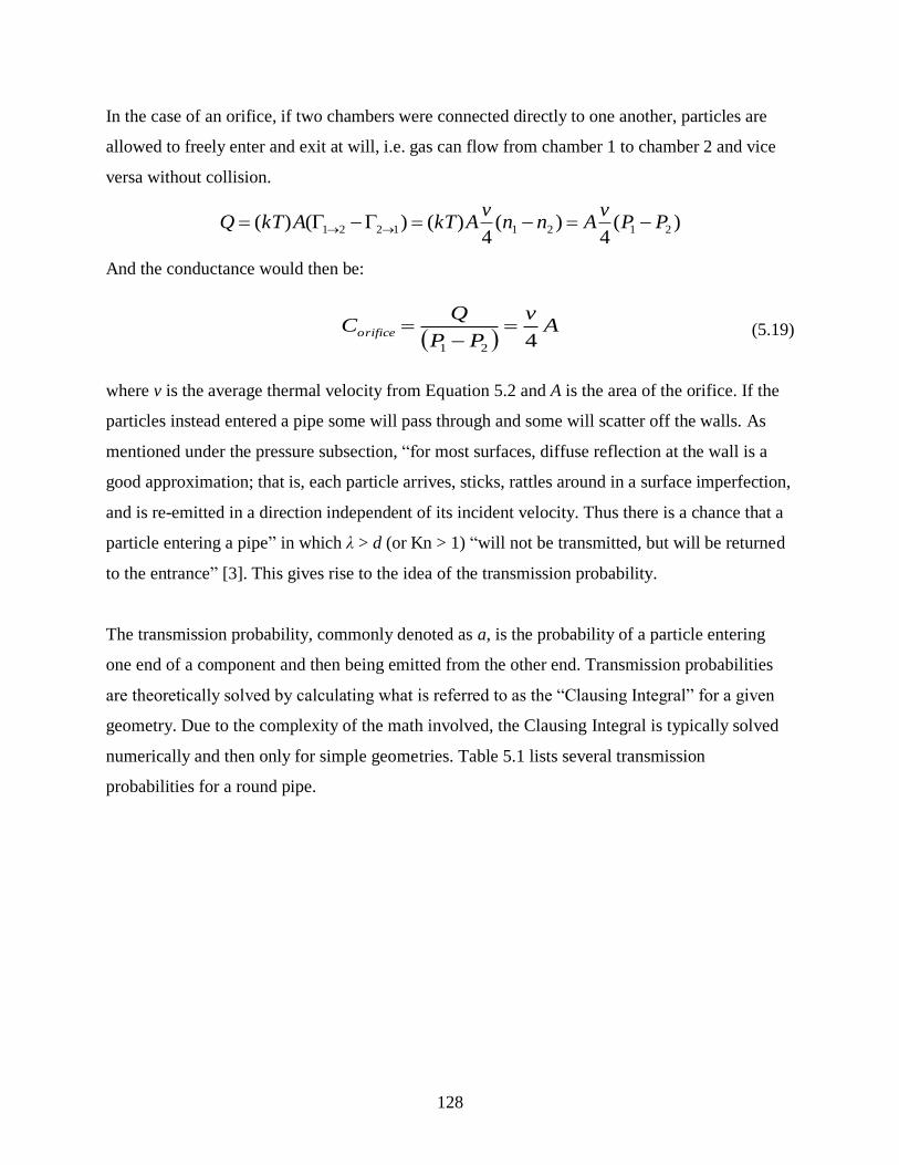
128
In the case of an orifice, if two chambers were connected directly to one another, particles are
allowed to freely enter and exit at will, i.e. gas can flow from chamber 1 to chamber 2 and vice
versa without collision.
)(4
)(4
)()()( 21211221 PPv
Annv
AkTAkTQ
And the conductance would then be:
(5.19)
where v is the average thermal velocity from Equation 5.2 and A is the area of the orifice. If the
particles instead entered a pipe some will pass through and some will scatter off the walls. As
mentioned under the pressure subsection, ―for most surfaces, diffuse reflection at the wall is a
good approximation; that is, each particle arrives, sticks, rattles around in a surface imperfection,
and is re-emitted in a direction independent of its incident velocity. Thus there is a chance that a
particle entering a pipe‖ in which λ > d (or Kn > 1) ―will not be transmitted, but will be returned
to the entrance‖ [3]. This gives rise to the idea of the transmission probability.
The transmission probability, commonly denoted as a, is the probability of a particle entering
one end of a component and then being emitted from the other end. Transmission probabilities
are theoretically solved by calculating what is referred to as the ―Clausing Integral‖ for a given
geometry. Due to the complexity of the math involved, the Clausing Integral is typically solved
numerically and then only for simple geometries. Table 5.1 lists several transmission
probabilities for a round pipe.
A
v
PP
QCorifice
421

129
Table 5.1: Transmission Probabilities for a round pipe of varying length to diameter ratio [3]
For a pipe, the conductance is then given by:
(5.20)
―Entrance and Exit effects,‖ which shall be discussed shortly, are included in these tabulations of
transmission probability values. Further details will be provided with regards to transmission
probability and molecular flow in a later section as the majority of the models will be based on
molecular flow. The reason for this basis will also be explained.
As an important side note, short tubes (which the GV may be considered, as will be noted later)
may have their conductances approximated by using the values from Table 5.1 (and interpolation
where necessary), or, as was the case with viscous flow, an aperture and tube can be used in
series. (The combination of conductances will be discussed momentarily.)
A
va
PP
QC
421

130
Alternatively, the Hanks-Weissberg model may be used. ―Few studies have been reported on gas
flow through short tube with very low pressure ratio‖ [28]. Hanks and Weissberg ―derived an
empirical equation of conductance for gas flow through short tube at conditions where the effects
of inertia and expansion are negligible‖ [28].
8
328/
88
32
83
16
64
9 32
22
D
LP
D
D
L
D
LvDCHW
(For the purpose of this thesis, the Hanks-Weisberg model will not be used as it is not considered
a standard or commonly used model.) A cursory examination of the formula seems to indicate
that it combines properties of both conductances formulas for molecular flow and viscous flow.
(Specifically, the left term is dependent only on diameter and average velocity as is the case with
molecular flow. The right term is dependent on the average pressure and diameter as was the
case with the formula for Poiseuille flow.) This technique is commonly used when trying to
calculate flows in the transition region.
5.1.10 Conductance in the Transition Region
―The theory of gas flow in the transition region is not well developed. The simplest treatment of
this region,‖ sometimes called the Knudsen method, essentially uses the principle of
superposition (although this is not technically the case as the different flow regimes cannot be
considered linear systems) and combines the effects of viscous and molecular flow to determine
the actual effect.
molecularviscoustransition QZQQ '
where for long circular tubes Z' is given by:
2095.31
2507.21
'd
d
Z

131
On the other hand, some texts [14] propose that correction factors may be adequate for capturing
the effect of gas-gas interactions on molecular flow.
(5.21)
Where the correction factor f, a function of pressure multiplied by diameter, is equal to:
(5.22)
for Ctube in Ls-1
, d in cm, and average pressure p̅ in mbar. [14]
Finally, the text by Hucknall and Morris differs from O‘Hanlon in stating (and/or providing
references that state) it is possible to consider the molecular flow to extend all the way up to the
region where Kn > 0.5 (as opposed to Kn > 1) and that ―the methods of viscous flow‖ can be
applicable up to Kn values of 0.3 (as opposed to Kn < 0.01) [14]. This would effectively limit the
region where neither viscous nor molecular flow models are representative of flow to only 0.3 <
Kn < 0.5. This thesis will treat this information as valid and attempt to apply the conductance
formulae for both flow regimes as well as correct for Knudsen flow (flow in the transition
region) wherever possible.
Finally, no theoretical model will provide ―exact‖ results for gas flow in the transition region.
Moreover, due to the random nature of particle movement, empirical data may not be identical
from test to test; however, it is only necessary for the values to be consistent (accurate) and
precise to the degree (or significant number of digits) that the instrumentation is able to measure.
As such, alternative methods are traditionally used to approximate or replicate empirical results.
These advanced models rely on the Monte Carlo method.
The Monte Carlo method actually refers to a general approach whereby many types of problems
can be ―solved‖ using random sampling (or number generation), a probability distribution that
encompasses all of the physics involved for the particular application, and a large enough
sampling run (or number of particles simulated) to obtain accurate results. It is a numerical
)(.,, dpfCC molectubeKntube
dp
dpdpdpf
2351
26202001)(
22

132
technique originally used in Los Alamos while performing work on neutron shielding. (It is now
used for many other purposes, including probabilistic risk assessment.) The Monte Carlo method
can be used to simulate the random nature of particle movement and thus can be used to
effectively reproduce gas particles moving in a system at low pressures.
5.1.11 A Note on other Models and Monte Carlo Simulations
It has been demonstrated that the Direct Simulation Monte Carlo (DSMC) ―method could predict
quite accurately the conductances in the transition regime of high Knudsen number.‖ [2] ―The
Monte Carlo technique uses a computer to simulate the individual trajectories of a large number
of randomly chosen molecules‖ and was a ―major breakthrough in the calculation of complex,
but practical, vacuum system elements such as elbows, traps, and baffles‖ [3]. However, the
accuracy of the Monte Carlo technique ―depends on the number of molecular trajectories used in
the calculation.‖ As such, ―a great deal of computational time is required for accurate solutions
to complex problems‖ [3]. As computer power increases Monte Carlo models (or in this case,
Molecular Dynamics models) to capture more of the physics inherent to the problem in addition
to increasing the number of particles simulated and decreasing the compute time.
Figure 5.7 provides a visual example of the Monte Carlo technique being applied to an elbow.
A transmission probability of 0.222 is found for an elbow when ―15 random molecules‖ are
simulated ―entering an elbow.‖ When a large number of particles was used (thus taking more
time), it yielded the actual transmission probability (as determined experimentally) of 0.31. [3]
Although, MC simulations have the great advantage of being able to simulate the entire
geometry of a system and modeling it all at once, the computational cost (namely, the time spent
multiplied by the expense of performing it) makes this tactic prohibitive. Instead, the common
practice is to ―approximate complex systems by combining cylindrical tubes, orifices, and baffle
plates‖ [3].

133
Figure 5.7: MC Simulation for an elbow (with only 15 particles) [3]
5.1.12 Combining Conductances
Once the conductances of the pipes and the GV have been estimated they can be combined in
series with capacity of the turbomolecular pump (i.e. the pump speed) to determine the ―effective
pumping speed‖ at the entrance to the main chamber. Again, this is the location where we
assume the location of the plane for which gas throughput it determined.
Conductances in parallel are given by:
...321 CCCCT
Conductances in series are given by:
(5.23)
It is absolutely critical to note that Equation 5.23 ―gives the value of conductance we would
measure if the elements were isolated from each other by large volumes‖ [3]. The physical
representation of this calculation (for only two elements in series) is provided in Figure 5.8 (a).
...1111
321
CCCCT

134
Figure 5.8: Conductance of two pipes in series that are (a) separated (or isolated) by a volume and
(b) NOT isolated by a volume (Note: the values are not equivalent) [3]
5.1.13 Exit and Entrance Effects
―The simple reciprocal rule does not work where we combine two conductances directly‖ [3].
Figure 5.8 shows two identical tubes (with l/d = 1 and a = 0.51423) connected in series, first in
isolation, case (a), then directly, case (b). Case (a) yields a combined transmission probability of
0.25712 when applying Eqn. 5.26 whereas case (b), which is now simply treated as pipe of l/d =
2, results in a probability of 0.35685. This is a difference of over 27.9% (as compared to the
actual value, 0.35685.) This occurs because the pressure is not distributed equally for both cases.
[3]
In case (a) the first tube is connected to ―a chamber of known pressure,‖ and because the
conductance is defined by the pressure drop across the component, ―the only place where the
pressure will differ is at the exit of the first tube‖ [3]. This pressure drop is termed the ―exit
loss.‖ When the two tubes are connected directly, this loss at the exit of the first tube is
eliminated. Combining conductances using Eqn. 5.26, as was done in case (a), induced error by
including this exit loss or ―exit impedance‖ twice as opposed to just the once. ―The choice
between an exact or approximate formula for the conductance of an individual pipe segment is
usually less important than the correction for the exit effect.‖ [3]

135
This can be corrected for by applying a different formula to instead solve for the combined
transmission probability. Oatley developed an infinite series expression based on the incoming
and outgoing particle flux for each element [3]. For simplicity‘s sake, only the final result is
shown:
1...1111
321
aaaa
Where the final term (the subtraction of 1) represents the exit pressure drop (or exit impedance).
This can also be rearranged to give:
...1111
3
3
2
2
1
1
a
a
a
a
a
a
a
a
Using this formula for combined probability to once more solve for the combination of two
l/d = 1 tubes in series yields an approximate result of a = 0.3460. This formula presents an error
of roughly 3%. [3]
Haefer expanded on Oatley‘s formula so that it ―extended to elements of differing diameters‖
and would thus be able to account for expansions and contractions. Haefer‘s addition theorem
―relates the total transmission probability of n elements a1→n to the transmission probability ai
and the inlet area Ai of each component‖ [3].
(5.24)
And the formula for overall conductance simply remains:
(5.25)
Note that additional terms (based on the inlets areas) are only applied in the combined
transmission probability formula when there is a contraction (or cross-sectional reduction in
area), not when there is an expansion (or increase in the inlet area of the next element). Also, the
overall formula for molecular conductance remains unchanged.
iiiiiiii
ii
n
ii
n
i
i
in
n
AAAA
AAa
a
Aa
a
A
11,11,
1,
1
1 111
1
1
for 0 and for 1 where
111111
nnncombined Av
aAv
aC4
)(4
)( 111

136
―The Oatley and Haefer formulas remove the biggest error in calculating the conductance of
combinations—the exit conductance drop at the end of each junction of equal diameter—but
neither formula corrects for entrance effects, that is, non-cosine or beamed entrance flux‖ [3].
5.1.14 Beaming Effects
When combining the two tubes from Figure 5.8 in series, although ―the pressures at the exit of
the first tube and the entrance to the second tube are‖ the same, ―the pressure is anisotropic.‖
This means that if a (directional) pressure gauge were placed at this point it would read higher
facing upstream than if it were facing downstream. Similarly, ―were it to face sideways, it would
also depend on whether it was located in the center of the tube or off-axis‖ [3].
The flux becomes increasingly anisotropic as it travels the length of the tube because of the
effect known as ―gas beaming.‖ This can best be explained by re-examining Figure 5.8. In case
(a), gas enters the second tube in the same manner it entered the first, with a random flux profile.
But in case (b), the flux entering the back half of the pipe is ―beamed.‖ Gas beaming is called an
entrance effect because the flux exiting the first element increases the transmission probability of
the next element that it enters. Typically this shift is small, and only represents an error of a few
percent. (This caused the deviation of 3% when using the Oatley method in the last example.)
Figure 5.9 illustrates the beaming effect by comparing the angular distributions of the flux
exiting a given pipe as a function of pipe length l and pipe diameter d.
Figure 5.9: Angular distribution of particles exiting tubes of various length-to-diameter ratios [3]

137
To clarify, Table 5.1 (and thus the Clausing Integral) incorporate beaming (or entrance) effects
into their values. Upon using the Haefer addition theorem, these effects are no longer accounted
for. The only way to compensate for this and to include beaming effects is to solve the Clausing
Integral for the exact geometry (which is oftentimes not possible) or to use a Monte Carlo
simulation (that is designed to take into account beaming effects).
Fortunately, entrance effects can typically be ignored in complex systems as most ―real systems
are made up of short tubes connected by elbows, traps, and so on.‖ Figure 5.9 shows ―that short
tubes have near-cosine exit flux.‖ Additionally, the ―elbows, baffles, chevrons, or the like will
also scatter molecules and shift the distribution toward cosine‖ [3].
For these reasons, the pumping stack has a ―maximum conductance when the elements are arranged
in increasing or decreasing order because the exit losses are the smallest and the beaming is the
greatest.‖ Alternating pipe sizes or introducing an elbow introduces wall scattering, which makes
the input to the following sections more like a Maxwell-Boltzmann gas (i.e. a gas with ―a cosine
distribution of scattered molecules‖). [3]
5.1.15 Conductance of Elbows
In addition to using the more accurate formulas developed by Oatley and Haefer, when
combining conductances it is recommended that the ―conductance of the actual configuration
should be calculated, because errors can creep in when components are mathematically
rearranged to simplify calculation‖ [3]. Although the initial conductance model assumes a simple
tubular geometry, successive models increasingly try to account for the actual geometry of the
system. However, not all the components in the pumping stack are a simple tube.
As discussed in Chapter 3, the arrangement of the pumping stack was designed with several
considerations in mind including maximizing conductance and minimizing pump wear.
Minimizing pump wear was given greater precedence thus the system was built using a right-
angle curved elbow in an attempt to isolate the pump from sputtering particles (debris).

138
Figure 5.11 provides for the comparison of a straight tube (left) and a ―non-degenerate‖ right-
angle elbow (right). (Non-degenerate means the diameter is fixed. Note that this elbow is not
curved but rather is the combination of two straight pipes joined together at a 90° angle.)
Examining Figure 5.11 and comparing the values for L/R = 2 from the figure on the left with the
figure on the right at the point where B/R = 1 for curve A/R = 1 (thus giving the same effective
length, i.e. L = A + B and A = B) they are approximately equivalent. Continued examination
shows this is true for the other corresponding points on the graph.
Figure 5.10: Transmission probability for a pipe (left) and an elbow (right) [3]
Other references support this same conclusion. ―Calculations show that a tube of right angle
bend and sections l1 = l2 leading to and from the bend, will have a transmission prob. Equivalent
to that of a straight tube of length L = l1 + l2 within a few percent.‖ And, more pertinently, ―in the
case of curved tubes having total length L, the transmission probability can be regarded as that of
an equivalent straight tube of length L.‖ [14]

139
Av
C
C
C pump
orifice
pump 4Ho
5.1.16 Additional Considerations Regarding the Pump Speed
The final consideration is incorporation of the pump speed into the overall equation for the
conductance of a system. It is easiest to find the actual pump speed, or ―effective pump speed,‖
S, by measuring the chamber pressure PV and system throughput Q:
(5.26)
Yet it is also known that S is equivalent to the combination of the (rated) pump speed and the
conductance of the connecting pipework (i.e. the pumping stack). Typically, this combination is
performed using Equation 5.23 such that:
(5.27)
All modeling of the gate valve and gas distribution were performed based off Equation 5.27 (the
exact derivations will be provided in a later section) as it considered the standard method [14, 3].
However, ―the formulas developed by Haefer and Oatley may be used to calculate the pumping
speed at the inlet of pipes connected to a pump.‖ This method, and the slight differences as
compared to combing the conductances of pipes, will be explained briefly.
A pump is ―simply considered to be a conductance of entrance area A and transmission
probability‖ that can be at maximum equal to the capture coefficient, Ho, of the pump [3].
―The Ho coefficient is the ratio of actual pumping speed to the maximum pumping speed of an
aperture of the same size in which no molecules are reflected‖ [3]. In other words, it is the pump
speed divided by the conductance of an orifice with equivalent inlet area:
Like with pipes, nonuniform gas distribution affects the measurement of pressures associated
with the pump and it also affects capture coefficient. ―The capture probability is a function of
arrival angle.‖ This also means that pumps are subject to entrance (or beaming) effects.
VPQS /
pipeworkpump CCS
111

140
If a pipe is connected to the inlet of a pump, ―the capture coefficient will increase‖ accordingly
and the pump will no longer have ―its ‗intrinsic‘ speed—that is, the speed it would have if
appended to an extremely large chamber.‖ (This assumes, of course, that the pump speed
documented by the manufacturer was determined using a ―large test dome‖ or a chamber of
significant size that the incoming flux has a cosine distribution. ―Test domes constructed from
pipes of the same diameter as the pump are criticized because the inlet flux is not cosine and the
resultant speed is not what is measured on a large chamber.‖) [3]
The physical reason the pump speed effectively increases is that ―molecules shot straight into the
pump will have a greater probability of being captured than will those arriving in a cosine
distribution, and because molecules bounce around—the ‗maze‘ effect‖ [3]. As mentioned
before, the main turbopump is connected via a right-angle curved elbow eliminating any benefit
from gas beaming. For these reasons, the actual pump speed of the pump may be equivalent to
the rated (or documented) value or may actually be less than reported (if the vendor value was
determined using a cylindrical test dome of equivalent inlet area). For all models, the pump
speed will be assumed to be equal to that provided in the pump literature, Figure 5.11 (shown on
the next page).

141
Fig
ure
5.1
1:
Pu
mp
Sp
eed
(o
r co
nd
uct
an
ce)
Cu
rve
for
TM
P 3
51
C f
or
va
ryin
g p
ress
ure
s

142
5.2 Assumptions Common to All Models
The tern gas dynamics is a technically a misnomer in that the dynamics of the system will not
actually be analyzed because the gas models are assumed to be time-independent; rather the gas
kinetics of the system are analyzed. We do this for two reasons. First, by assuming the system is
in steady-state, the problem becomes a simple energy balance problem and is significantly easier
to solve. Second, the actual time scale of the fluctuations is such that the steady-state assumption
is valid. The time it takes for the gas to reach equilibrium and reach a constant pressure is less
than the time it takes for the Gate Valve (GV) motor to physically move the gate to a different
position (which according to the manual is three seconds to go from full open to close or vice
versa). This has been verified qualitatively by tracking the fluctuation in pressure as the position
is reset using both a pressure sensor located off of the cluster flange to the primary chamber and
the pressure sensor controlling the gate valve which is attached to the reducing cross located
adjacent to the gate valve.
It is also assumed that the gas is at constant temperature so it is now valid to consider this a mass
balance problem, the exact reason for this will be shown in the ―note on units‖ section. Other
methods of energy transfer, such as radiation or thermal conductivity and convection will not be
considered in detail in this review as they were ignored for the purposes of creating first-order
analytical models for system analysis. Advanced molecular dynamics (MD) models, which are
not within the scope of this thesis, may later be developed from first principles to take these
processes into account accordingly.
When calculating the molecular flow models some assumptions were made with regards to the
geometry of the Gate Valve gate (GV gate) that are common to all models. According to the
schematic provided by the manufacturer, the GV gate inlet area is slightly larger than the
surrounding pipework when ―full open.‖ (The GV orifice has an inner diameter (I.D.) of 3.94
inches whereas all other 6-inch CF piping and the entrance and exit to the GV have an I.D. of
3.854 inches. This ―slit-like expansion‖ could account for some of the miscellaneous losses in
conductance of the system. The reason being that it would be very easy for particles to become
―trapped‖ (or effectively stalled) in these areas for a short time thus further reducing the
transmission probability of the GV.

143
It is thought that film production would not typically occur in the range requiring the GV to be
opened more than 97% because there is less reliability in measurements of any system at its
upper or lower operational bounds. Therefore additional effort to consider operation in this
region was not deemed necessary by the author.
Finally, the conductance used for the GV orifice under molecular flow conditions was not the
same as that provided in the manual for that piece of equipment. At this time it is uncertain as to
how exactly VAT determines this property as it would seem to require a significantly higher than
ambient temperature contributing to the velocity of the gas particles. Instead, the conductance
was simply based on Equation 5.19 and the inlet area of the pumping stack.
There are some additional constraints and limitations to theoretical models detailed below.
Theoretical models do not:
Account for the internal geometry of the chamber. (This includes the reduction in
conductance due to the fixtures in the system as well as effects related to the position at
which processing gas is introduced.)
Account for contraction from 10-inch CF chamber to the 6-inch CF reducing nipple.
Account for miscellaneous losses in conductances due to the ports on the reducing cross,
gaps by the GV gate, etc.
Account for Ar-O2 mixes. (Experimental data and models are for Argon gas only.)
5.3 A Note on Units
The standard unit for throughput is Pa-m3/s (in SI units) or Torr-L/s, this is a volumetric unit.
However, the mass flow meters provide the gas input in terms of sccm (standard cubic
centimeters per minute) which are not technically volumetric units but instead are units of mass
flow. This is because sccm units assume STP conditions, in other words they specify a
temperature which for STP condition is 0°C. For the purposes of this analysis, units of mTorr-L/s
are used to measure throughput. This is simply because the operating pressures are measured in
terms of mTorr. At STP conditions a simple conversion can be used: 1 sccm is approximately
equal to 12.6667 mTorr-L/s.

144
However, these units must be adjusted to account for the actual temperature and the resulting
expansion in gas volume. The temperature is considered to be ambient temperature which was
set at 75° F. (This was the average temperature in the room the day in which experimental results
were measured.) In determining the change in throughput it is known that the pressure is held
constant and that the time scale will remain the same, therefore only the change in volume will
affect the value of the throughput. The volume will change as a result of the temperature change,
and the correction for temperature is simple once Charles‘ law, which comes from the Ideal Gas
Law, is applied:
2
2
1
1
T
V
T
V for N, P held constant
(Note that N is constant because the actual number of gas particles is unchanged, only the
volume required to contain them has changed.)
Substituting throughput into Charles‘ law yields:
(5.28)
Again, the whole point of this exercise is to ensure that the pressure measurements of the
Baratron gauge and the ambient temperature of the room can be used to accurately determine the
amount of gas leaving the chamber per unit time so that it can be compared to the amount
injected into the system.
5.4 Prerequisite and Ancillary Calculations
Before delving into the theoretical models, the results of several prerequisite and a few ancillary
calculations will be discussed. The prerequisite calculations were required in order to determine
what conductance calculations would be valid for the operating range prescribed by film
fabrication. The supplemental information furthers the soundness of the models while also
exposing some of their constraints. The necessary equations have already been explained in the
previous section and only their application and results will detailed herein. The conversions used
in the Excel calculations will not be discussed but units are noted (where applicable). For
convenience sake, all relevant Tables will simply be placed at the end of this section.
1
212
2
2
1
1
T
TQQ
T
Q
T
Q

145
The mean free path of the gas particles must first be calculated in order to determine what regime
the Gas Distribution system is operating within. The mean free path is then used to calculate the
Knudsen number for the chamber region and for the pumping stack (i.e. the associated pipe work
used to pump down on the system). Both the mean free path and Knudsen number were solved
using Equation 5.9 which related them to the pressure in the chamber. Comparison of the results
in Table 5.4 with Figure 5.6 shows that the gas in the pipe (or pumping stack) will be
characterized by transition flow over the entire predicted operating range. Interestingly, this
comparison also indicated that the particles in the main chamber will transition from viscous
flow to transition flow as the pressure drops below 13 mTorr (approximately).
As an auxiliary calculation, the effects of mixing Argon and Oxygen gases on the mean free path
and Knudsen numbers were shown in Table 5.5. These values were calculated using Equation
5.5 and are provided only as a supplement as all experimental analysis and theoretical models
used pure Argon for the conductance calculations. It should be noted that Oxygen gas has a
smaller mean free path than Argon gas (at the same temperature) and at higher partial pressures
will cause the mixed gas to pass from the transition region to the viscous region at a lower
pressure (i.e. more quickly) as compared to Argon gas flow.
Based on the Knudsen numbers in Table 5.4 and the fact that viscous model could apply to
regions up to Kn = 0.3, a viscous model was the first model to be proposed [14]. However, as
seen by the Equation 5.14, it was impossible to calculate the conductance of an orifice, in this
case the GV, without knowing both the upstream and downstream velocity. At this point flow
models began to focus on the molecular flow regime as a basis. Still, in case other viscous
conductances would later be applied (such as Equation 5.13), the prerequisite information was
determined. This included: calculation of the entrance length, Reynolds‘ number, dynamic
viscosity, and average velocity. This required the use of Equations 5.12, 5.10, 5.11, and 5.2,
respectively. The results are provided in Tables 5.2 and 5.3. Note that the entrance length is very
small (as compared to a pipe length greater than a foot) and thus the flow would be fully-
developed (were it actually in the viscous flow regime). Additionally the Reynolds‘ number is
extremely small, suggesting that Reynolds‘ number may not actually applicable for this flow
situation.

146
As a supporting calculation, the speed of sound (the gases of interest) was also calculated (using
Equation 5.15) so that the Mach number could be determined (using Equation 5.16) to address
the question of compressibility. As long as the Mach number was less than one third (Equation
5.18), the effects of gas compressibility could be ignored. The results shown in Table 5.6 show
that gas compressibility is negligible over the operational range of the system, approaching a
Mach value one tenth of what is considered to indicate compressibility and even then only at the
lower limits of the system‘s pressure range.
Finally, the possibility of choked flow was also analyzed. (This could be considered as a means
of double-checking previous calculations as the flow should not be choked given such low
Reynolds‘ and Mach numbers.) Equation 5.17 was used to calculate the GV area at which
choked flow would take effect given a set flow rate and pressure. The results are presented in
Table 5.7. These results may seem counterintuitive at first and require some additional
explanation.
For a given flow rate, choked flow will be more likely to occur as the required chamber pressure
is lowered, this is because more gas must be evacuated in the same amount of time and through
the same area to maintain the lower pressure. Similarly, at a given pressure a higher flow rate
will require more gas to be forced out of the system. Calculations indicate that choked flow only
occurs when the GV is less than 2% open and only for pressures at the lower limit of where the
system is capable of operating. In fact, all these values are outside the desired range in which the
GV would operate due to stability and reproducibility concerns. (In both Tables 5.6 and 5.7
values that could not later be achieved experimentally, and resulted in non-real values in the
theoretical models, were omitted.) The limited range of control for the GV system with respect to
operational pressure (most likely caused by a lower conductance than expected) will be
discussed further in Chapter 6.

147
REYNOLDS NUMBER AND ENTRANCE LENGTH
Qin = 10 sccm
R le [in]
0.174070542 0.037907551
Qin = 20 sccm
R le [in]
0.348141085 0.075815102
Qin = 40 sccm
R le [in]
0.69628217 0.151630204
Table 5.2: Reynolds Numbers and Entrance Length for Fully-Developed Flow for various
throughputs
DETERMINED VALUES
Avg. velocity, v [m/s] 396.7770483 (for temperature of 75°F)
Speed of sound, Usound [m/s] 321.3177526 (for Ar) and 294.3035852 (for O2)
Dynamic viscosity, η [Pa-s] 2.23112E-05
Table 5.3: Average velocity, Speed of Sound, and Viscosity to be used in other calculations

148
MEAN FREE PATH AND KNUDSEN NUMBER
Pv [mTorr] λ [in] Knpipe Knchamber
0.5 4.114552903 1.073175 0.261075692
1 2.057276452 0.536587 0.130537846
1.5 1.371517634 0.357725 0.087025231
2 1.028638226 0.268294 0.065268923
2.5 0.822910581 0.214635 0.052215138
3 0.685758817 0.178862 0.043512615
3.5 0.587793272 0.153311 0.037296527
4 0.514319113 0.134147 0.032634461
4.5 0.457172545 0.119242 0.02900841
5 0.41145529 0.107317 0.026107569
5.5 0.374050264 0.097561 0.023734154
6 0.342879409 0.089431 0.021756308
6.5 0.316504069 0.082552 0.020082746
7 0.293896636 0.076655 0.018648264
7.5 0.274303527 0.071545 0.017405046
8 0.257159556 0.067073 0.016317231
8.5 0.242032524 0.063128 0.015357394
9 0.228586272 0.059621 0.014504205
9.5 0.216555416 0.056483 0.013740826
10 0.205727645 0.053659 0.013053785
10.5 0.195931091 0.051104 0.012432176
11 0.187025132 0.048781 0.011867077
11.5 0.178893604 0.04666 0.011351117
12 0.171439704 0.044716 0.010878154
12.5 0.164582116 0.042927 0.010443028
13 0.158252035 0.041276 0.010041373
13.5 0.152390848 0.039747 0.00966947
14 0.146948318 0.038328 0.009324132
14.5 0.141881135 0.037006 0.00900261
15 0.137151763 0.035772 0.008702523
15.5 0.132727513 0.034619 0.008421797
16 0.128579778 0.033537 0.008158615
16.5 0.124683421 0.03252 0.007911385
17 0.121016262 0.031564 0.007678697
17.5 0.117558654 0.030662 0.007459305
18 0.114293136 0.02981 0.007252103
18.5 0.111204133 0.029005 0.0070561
19 0.108277708 0.028241 0.006870413
19.5 0.105501356 0.027517 0.006694249
20 0.102863823 0.026829 0.006526892
Table 5.4: Mean free path and Knudsen Numbers for Argon gas as a function of pressure
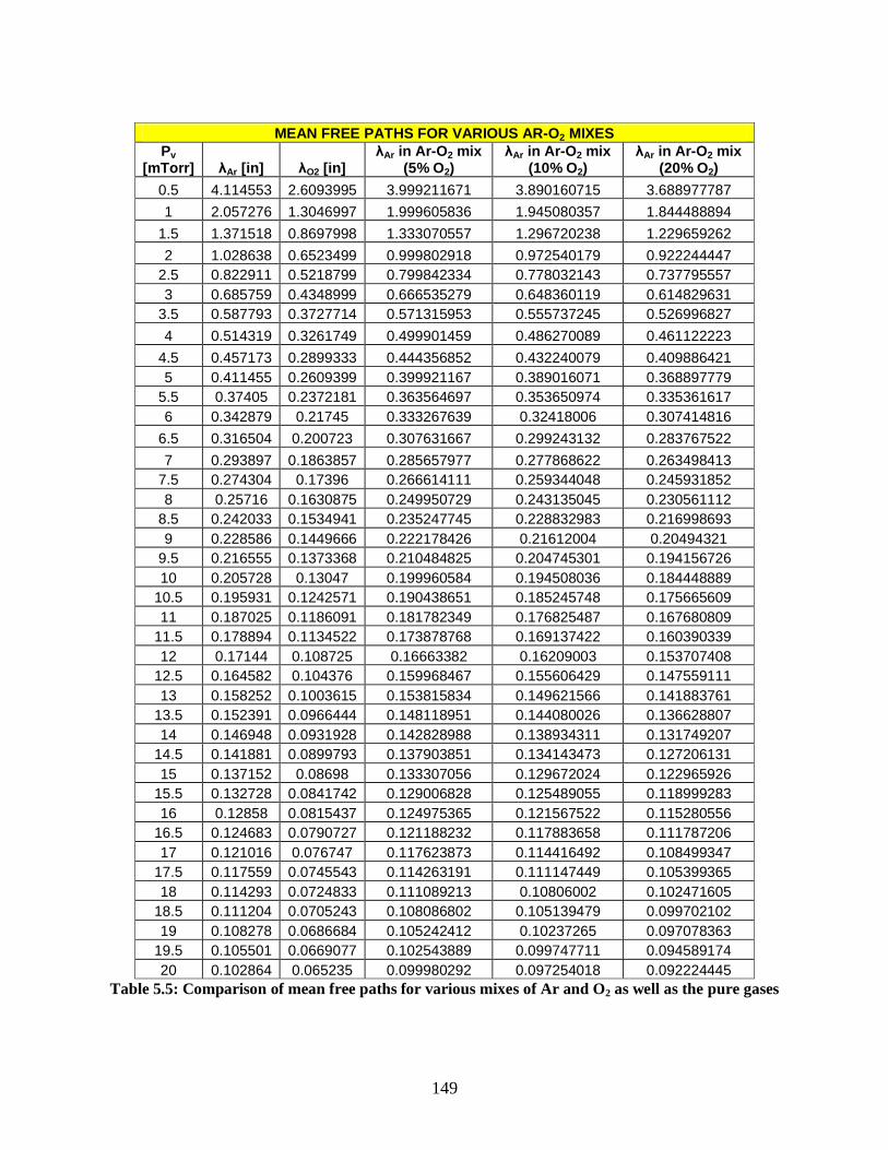
149
MEAN FREE PATHS FOR VARIOUS AR-O2 MIXES
Pv [mTorr] λAr [in] λO2 [in]
λAr in Ar-O2 mix (5% O2)
λAr in Ar-O2 mix (10% O2)
λAr in Ar-O2 mix (20% O2)
0.5 4.114553 2.6093995 3.999211671 3.890160715 3.688977787
1 2.057276 1.3046997 1.999605836 1.945080357 1.844488894
1.5 1.371518 0.8697998 1.333070557 1.296720238 1.229659262
2 1.028638 0.6523499 0.999802918 0.972540179 0.922244447
2.5 0.822911 0.5218799 0.799842334 0.778032143 0.737795557
3 0.685759 0.4348999 0.666535279 0.648360119 0.614829631
3.5 0.587793 0.3727714 0.571315953 0.555737245 0.526996827
4 0.514319 0.3261749 0.499901459 0.486270089 0.461122223
4.5 0.457173 0.2899333 0.444356852 0.432240079 0.409886421
5 0.411455 0.2609399 0.399921167 0.389016071 0.368897779
5.5 0.37405 0.2372181 0.363564697 0.353650974 0.335361617
6 0.342879 0.21745 0.333267639 0.32418006 0.307414816
6.5 0.316504 0.200723 0.307631667 0.299243132 0.283767522
7 0.293897 0.1863857 0.285657977 0.277868622 0.263498413
7.5 0.274304 0.17396 0.266614111 0.259344048 0.245931852
8 0.25716 0.1630875 0.249950729 0.243135045 0.230561112
8.5 0.242033 0.1534941 0.235247745 0.228832983 0.216998693
9 0.228586 0.1449666 0.222178426 0.21612004 0.20494321
9.5 0.216555 0.1373368 0.210484825 0.204745301 0.194156726
10 0.205728 0.13047 0.199960584 0.194508036 0.184448889
10.5 0.195931 0.1242571 0.190438651 0.185245748 0.175665609
11 0.187025 0.1186091 0.181782349 0.176825487 0.167680809
11.5 0.178894 0.1134522 0.173878768 0.169137422 0.160390339
12 0.17144 0.108725 0.16663382 0.16209003 0.153707408
12.5 0.164582 0.104376 0.159968467 0.155606429 0.147559111
13 0.158252 0.1003615 0.153815834 0.149621566 0.141883761
13.5 0.152391 0.0966444 0.148118951 0.144080026 0.136628807
14 0.146948 0.0931928 0.142828988 0.138934311 0.131749207
14.5 0.141881 0.0899793 0.137903851 0.134143473 0.127206131
15 0.137152 0.08698 0.133307056 0.129672024 0.122965926
15.5 0.132728 0.0841742 0.129006828 0.125489055 0.118999283
16 0.12858 0.0815437 0.124975365 0.121567522 0.115280556
16.5 0.124683 0.0790727 0.121188232 0.117883658 0.111787206
17 0.121016 0.076747 0.117623873 0.114416492 0.108499347
17.5 0.117559 0.0745543 0.114263191 0.111147449 0.105399365
18 0.114293 0.0724833 0.111089213 0.10806002 0.102471605
18.5 0.111204 0.0705243 0.108086802 0.105139479 0.099702102
19 0.108278 0.0686684 0.105242412 0.10237265 0.097078363
19.5 0.105501 0.0669077 0.102543889 0.099747711 0.094589174
20 0.102864 0.065235 0.099980292 0.097254018 0.092224445
Table 5.5: Comparison of mean free paths for various mixes of Ar and O2 as well as the pure gases

150
MACH NUMBER AND COMPRESSIBILITY
Qin = 10 sccm Qin = 20 sccm Qin = 40 sccm
Pv [mTorr] U U U
0.5 1 1.5 2 0.028777178
2.5 0.023021742 3 0.019184785 0.03836957
3.5 0.016444102 0.032888203 4 0.014388589 0.028777178 4.5 0.012789857 0.025579714 5 0.011510871 0.023021742 5.5 0.010464428 0.020928857 6 0.009592393 0.019184785 6.5 0.008854516 0.017709033 7 0.008222051 0.016444102 0.032888203
7.5 0.007673914 0.015347828 0.030695656
8 0.007194294 0.014388589 0.028777178
8.5 0.006771101 0.013542201 0.027084403
9 0.006394928 0.012789857 0.025579714
9.5 0.006058353 0.012116706 0.024233413
10 0.005755436 0.011510871 0.023021742
10.5 0.005481367 0.010962734 0.021925469
11 0.005232214 0.010464428 0.020928857
11.5 0.005004727 0.010009453 0.020018906
12 0.004796196 0.009592393 0.019184785
12.5 0.004604348 0.009208697 0.018417394
13 0.004427258 0.008854516 0.017709033
13.5 0.004263286 0.008526571 0.017053142
14 0.004111025 0.008222051 0.016444102
14.5 0.003969266 0.007938532 0.015877064
15 0.003836957 0.007673914 0.015347828
15.5 0.003713184 0.007426368 0.014852737
16 0.003597147 0.007194294 0.014388589
16.5 0.003488143 0.006976286 0.013952571
17 0.00338555 0.006771101 0.013542201
17.5 0.00328882 0.006577641 0.013155281
18 0.003197464 0.006394928 0.012789857
18.5 0.003111046 0.006222093 0.012444185
19 0.003029177 0.006058353 0.012116706
19.5 0.002951505 0.005903011 0.011806022
20 0.002877718 0.005755436 0.011510871
Table 5.6: Mach number at pertinent throughputs and pressures
(Non-real values—i.e. those not within the operational range of the system—are omitted)

151
CHOKED FLOW LIMITS
Qin = 10 sccm Qin = 20 sccm Qin = 40 sccm
PV [mTorr] %GV %GV %GV
0.5 1 1.5 2 0.011635384
2.5 0.009308307 3 0.007756923 0.015513845
3.5 0.006648791 0.013297582 4 0.005817692 0.011635384 4.5 0.005171282 0.010342564 5 0.004654154 0.009308307 5.5 0.004231049 0.008462098 6 0.003878461 0.007756923 6.5 0.003580118 0.007160236 7 0.003324395 0.006648791 0.013297582
7.5 0.003102769 0.006205538 0.012411076
8 0.002908846 0.005817692 0.011635384
8.5 0.002737737 0.005475475 0.01095095
9 0.002585641 0.005171282 0.010342564
9.5 0.002449555 0.004899109 0.009798218
10 0.002327077 0.004654154 0.009308307
10.5 0.002216264 0.004432527 0.008865055
11 0.002115524 0.004231049 0.008462098
11.5 0.002023545 0.00404709 0.00809418
12 0.001939231 0.003878461 0.007756923
12.5 0.001861661 0.003723323 0.007446646
13 0.001790059 0.003580118 0.007160236
13.5 0.001723761 0.003447521 0.006895042
14 0.001662198 0.003324395 0.006648791
14.5 0.001604881 0.003209761 0.006419522
15 0.001551385 0.003102769 0.006205538
15.5 0.00150134 0.00300268 0.00600536
16 0.001454423 0.002908846 0.005817692
16.5 0.00141035 0.002820699 0.005641398
17 0.001368869 0.002737737 0.005475475
17.5 0.001329758 0.002659516 0.005319033
18 0.00129282 0.002585641 0.005171282
18.5 0.001257879 0.002515759 0.005031517
19 0.001224777 0.002449555 0.004899109
19.5 0.001193373 0.002386745 0.004773491
20 0.001163538 0.002327077 0.004654154
Table 5.7: GV position (as a percentage) at which choked flow conditions take effect as based on
pressure and flow rate (non-real values omitted)

152
5.5 Methodology and Derivations
The gas flow regimes and the corresponding conductance calculations as well as the assumptions
which lay the foundation for the models have been established; the exact derivations for the
various models may now be provided. Note that all unit conversions are accounted for in the
Excel spreadsheet used to calculate all of the models. Again, conversions will not be discussed in
the derivations and units are only noted in the cases of particular formulas/plots that differ from
the units typically used in the models.
5.5.1 Simple Tubular Geometry Model
This model combines all the components of the pumping stack and treats them as a single tube of
constant diameter with the GV itself considered an aperture (or orifice) of varying size. The GV
is considered to be in series with the pump and the pumping stack.
Derivation:
Assume steady-state throughput: outin QQQ
Based on Equations 5.23 and 5.27 the effective pumping speed S will be determined by using
the combination of conductances for elements in series except now the conductance of the GV
will be considered an additional term in that series such that:
GVpipeworkpump CCCS
1111
And when combined with Equation 5.26 this yields:
(5.29)
For this model assume Cpump is constant and use fixed Q. PV is the independent variable.
The value for Cpipework and CGV must now be determined.
Q
P
CCC
V
GVpipeworkpump
111

153
According to Equation 5.20, Av
aC pipework4
and A = Amax where Amax is the area of the fully
unobstructed pipe (which is also assumed to be the maximum for the GV) and transmission
probability a is determined based on the l/d ratio and Table 5.1 (using interpolation where
necessary). Thus, Cpipework is a constant value.
From Equation 5.19, GVGV Av
C4
(because the GV is treated as a circular orifice) and AGV is the
dependent variable. Substituting for CGV back into Equation 5.29 yields:
Q
P
vACC
V
GVpipeworkpump
4111
Upon rearranging this becomes:
pipeworkpump
V
GV CCQ
P
vA
1141
or
1
11
4
pipeworkpump
VGV
CCQ
PvA
By solving for AGV and then dividing both sides by Amax the equation can be rewritten in terms of
the percentage the GV is open (%GV).
(5.30)
1
max
114%
pipeworkpump
VGVGV
CCQ
P
vA
A

154
5.5.2 Complex Geometry Model (Tubular Geometry with Expansions and Contractions)
This model provides an alternate geometry to that of Model 1 (the simple tube geometry). It
accounts for expansions and contractions by using the Haefer method for combining
transmission probabilities. More importantly this has the added benefit that the exit loss is no
longer included multiple times. This model will also allow for the GV to be treated as either an
orifice or as a short tube of varying sizes (which better represents the actual geometry).
This model will start from the same basis as the previous model, but this time CGV and Cpipework
are combined into a joint term denoted Ccombined.
So that now:
(5.31)
It is now easiest to think of the geometry of the pumping stack in terms of three different sections
(instead of the single tube and orifice from before).
Section 1 corresponds to: the length of the reducer nipple, plus the cross, plus one third the
length of the GV (which is estimated to be the GV entrance region which is of constant size and
not affected by the gate itself). A1 and a1 are the corresponding constants.
Section 2 corresponds to: the actual GV gate region (again considered to be one third the length
of the entire segment). This is the area of interest with regards to the gate valve as both A2 and a2
will vary depending on the position of the gate shutter.
Section 3 corresponds to: one third the length of the GV (which is estimated to be the GV exit
region; equivalent in nature to that of the entrance) plus the length of the elbow (which can be
treated as straight tube as explained in previous sections). A3 and a3 are constants. Figure 5.12
provides an illustration of the new geometry. (In the picture the GV is partially closed.)
Q
P
CCS
V
combinedpump
111

155
Figure 5.12: Three region model (with partially closed GV) to be evaulated using Haefer’s Addition
Theorem [3]
Applying Haefer‘s addition theorem (Equation 5.24) to this new geometry yields:
iiiiiiii
ii
iii
i
i
AAAA
AAa
a
Aa
a
A
11,11,
1,
2
1 1
3
131
31
1
for 0 and for 1 where
111111
Note that A1 = A2 = A3 = Amax when the GV is fully open, and that for a partially closed GV that
A2 < A1 and A3 > A2. This means that 12,1 and 03,2 so this becomes:
123
3
32
2
21
1
131
31
1
1111111111
AAa
a
Aa
a
Aa
a
Aa
a
A
Solving for 31a , simplify by multiplying both sides by A1.
12
1
3
3
3
1
2
2
2
1
1
1
31
31 111111
AAA
a
a
A
A
a
a
A
A
a
a
a
a
A1 = A3 is used to cancel the term A1/A3. The fractions are then split to take the form:
111
11
1
aa
a
The equation now takes the form:
111
11
11
11
2
1
322
1
131
A
A
aaA
A
aa

156
After simplification:
(5.32)
At this point, for easier notation, new definitions will be applied: Let A2 = AGV, acombined = a1→3,
and aGV = a2 so that when using Equation 5.25 Ccombined is now given as:
14
Av
aC combinedcombined where A1 = Amax
Note that aGV is a dependent variable based on the GV diameter dGV (and thus the area AGV) and
acombined is dependent on aGV and on AGV (which again is related to dGV). (This will be explained
in further detail later, because of this dependence %GV will later be set as the independent
variable and thus making PV the dependent variable.)
Going back to Equation 3.31, Ccombined can be rewritten as:
1
1
pump
Vcombined
CQ
PC
Upon substitution:
(5.33)
Solving for acombined:
(5.34)
Combining Equations 5.33 and 5.32 yields the relation:
pump
V
GVGVcombined CQ
PvA
aaA
A
aa
1
42
11111
3
1
1
21111
322
1
131
aaA
A
aa
1
1
141
pump
Vcombined
CQ
P
vAa
1
1
1
4
pump
Vcombinedcombined
CQ
PA
vaC

157
And given A1 = Amax and that %GV = AGV/Amax this becomes:
pump
V
GVGV CQ
PvA
aaa
1
42
111
%
11
31
Solving for %GV:
(5.35)
Or rearranged:
(5.36)
5.5.3 A Note on Transmission Probabilities
Initially Table 5.1 and interpolation was used to determined aGV for the first few models. The
transmission probability data for varying l/d ratios was later fit by Hyunsu Ju and a formula was
determined:
(5.37)
Where we will determine dGV based on %GV as follows:
(5.38)
(Again, the diameter is based on the GV orifice being treated as circular area.)
So as to avoid iteration, from this point forward %GV will be set as the independent variable and
PV as the dependent variable (additional graphs have also been provided in the Appendices with
the axes reversed so as to provide a simple visual comparison to earlier work.)
1
31
1 2111
4%
aaCQ
PvAa
pump
VGVGV
vAaaaCQP
GVGVpump
V
412
111
%
11
max31
)]070412.0)/(ln(exp[1
11
GV
GVdl
a
)(%44% max
max
2
max
GVGV
GVGV
GV
Ad
A
d
A
A

158
Additional corrections were also later introduced to the models which could be used to account
for changes in pump speed with respect to PV and to account for viscous effects in the transition
region.
5.5.4 Pump Correction
Turbomolecular pump speed varies based on operating pressure because there are only a limited
number of particles that it can remove (or capture) from the system at a time. The manufacturer
provided a ―pump curve‖ which shows the expected (or rated) pump capability as a function of
pressure over the operational range of the pump. This is provided as is in Figure 5.11. As noted
earlier, the pump curve is assumed to be valid without independent verification. By visual
inspection (and based on the axes) the pump curve is recognized as being related to some form of
logarithmic curve. (No formula was stated for the curve.)
Based on the pump curve shown in Figure 5.11, it was hypothesized that reduction in the pump
speed caused by increased pressure would have a minimal affect on the conductance of the
system over the initially predicted operating range of 2–20 mTorr.
In order to gauge the effect, points were extrapolated from the curve (using the logarithmic
fraction-ratio method) and used to determine approximate pump speed values at different
pressures. As a first order estimate, only a manually discretized correction was applied to the
simplest geometry model. The original discretization applied is shown in Table 5.2. This
correction induced noticeable errors in the plots of the conductance (because the pump curve had
not been divided, or discretized, into small enough slices); however, it was still sufficient in
highlighting the areas and degree to which the pump correction would affect the model.
A second correction was then made (only applicable to the pressure range of interest) and plotted
in Excel where a polynomial fit was then applied to the curve. This new fit was used for all
further models but required the use of iteration in Excel. The equation yielded is given as:
(5.39)
47.3469524.663.21496.00027.0 234 VVVVpump PPPPC
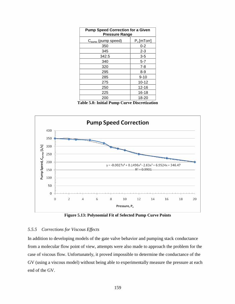
159
Pump Speed Correction for a Given Pressure Range
Cpump (pump speed) Pv [mTorr]
350 0-2
345 2-3
342.5 3-5
340 5-7
320 7-8
295 8-9
285 9-10
275 10-12
250 12-16
225 16-18
200 18-20
Table 5.8: Initial Pump Curve Discretization
Figure 5.13: Polynomial Fit of Selected Pump Curve Points
5.5.5 Corrections for Viscous Effects
In addition to developing models of the gate valve behavior and pumping stack conductance
from a molecular flow point of view, attempts were also made to approach the problem for the
case of viscous flow. Unfortunately, it proved impossible to determine the conductance of the
GV (using a viscous model) without being able to experimentally measure the pressure at each
end of the GV.

160
Thus the first attempt to account for the possibility of viscous flow continued to treat the GV as
an orifice subject to molecular flow conditions and treated the simple tube geometry as a long
pipe subject to laminar viscous flow corresponding to Equation 5.13. (In other words, Equation
5.13 was used in place of Equation 5.20.) This alternate conductance was then combined in
series and rest of the derivation proceeded as normal once again ending with Equation 5.30.
This method was deemed unacceptable and an alternate correction was used to account for
potential viscous effects. This method relied on the Knudsen correction for transition flow which
was shown in Equations 5.21 and 5.22. The use of the correction will now be explained further
as its integration is more complex.
Starting from Equation 5.21, Ctube, molec will be considered to be equivalent to the previously
determined Ccombined from Equation 3.33 but Ctube, Kn will then be considered to be the actual
conductance term, C′combined, measured in the system such that:
)()( , , dpfCdpfCCC combinedmolectubeKntubecombined
This makes sense as the conductance for the piping and the GV is effectively being ―magnified‖
(or increased by some factor) by the gas-gas collisions increasing the transmission probability so
that:
)(4
' max dpfAv
aC combinedcombined
And as before in Equation 5.33:
1
1'
'
11
pump
Vcombined
V
combinedpump CQ
PC
Q
P
CC
Continuing in this fashion, a′combined will now be solved for:
(5.40)
The ′ merely denotes that this is the formula including the correction for viscous effects.
)(
11411
1 dpfCQ
P
vAa
pump
Vcombined

161
Substitute a′combined for acombined (by combining Equations 5.32 and 5.40) to get:
2111
%
11
31
aaaa GVGVcombined
This then becomes:
))((1
42
111
%
1max
31
dpfCQ
PvA
aaa pump
V
GVGV
Rearranged this is:
(5.41)
Where again, the ′ denotes that this is the formula including the correction for viscous effects.
Note that, because the Knudsen correction factor f is dependent on the average pressure (which is
assumed to be equal to PV), this process requires iteration. (If the pump correction detailed
previously is then applied, this equation would instead require two loops of iteration—one for
pressure and one for pump speed.)
5.5.6 Reason for Flux Distribution Corrections
All previous models treated the GV region as a variable area that maintained a circular shape.
This was done in order to use the conductance formulas and transmission probabilities for
standard smooth circular pipework. However the actual geometry of the GV corresponds to a
progressing series of circle segments as shown in Figure 5.14. In order to develop a more
accurate model, corrections were then made in an attempt to correct for the geometry and to
achieve the proper transmission probabilities.
)(
1412
111
%
11
max31 dpfvAaaaCQP
GVGVpump
V

162
Figure 5.14: Actual Gate Valve geometry versus that which was modeled
To better simulate the actual geometry present in the throat of the pumping stack, the
transmission probability must be reduced in order to account for the portion of gas flux that
would impinge on the sliding gate (of the gate valve) and be reflected back into the pipe. The
ratio of flux not blocked by the gate to the total flux of the pipe is multiplied by the original
transmission probability (which comes from Equation 5.37) in order to better estimate the actual
transmission probability. (Thus only the portion of the incident flux not coming into contact with
the gate would be considered to contribute to the conductance of the remainder of the pumping
stack.)
Technically, this would mostly likely overestimate the total number of particles that do not pass
through the pipe because in real world circumstances these particles would also have some
probability of being reflected back into the throat of the pipe or again into the gate. (Developing
another infinite series expression, a la Oatley, would solve this problem.) Instead ignoring this
effect should then under value the actual transmission probability and should technically give
rise to a more conservative model. The actual results as discussed in Chapter 6 will show this
was not the case.
The actual amount of the flux being blocked (or impacting on the GV gate) and the total flux
must now be calculated. For gas in a smooth circular pipe it is known that the flux profile will
generally take the shape of a cosine distribution. The exact nature of this shape depends on the

163
pipe, primarily the length-to-diameter ratio (as was shown in Figure 5.9) and the resulting gas
beaming (that takes place as the gas proceeds down the length of the pipe). Longer pipes will
possess a finer distribution of particles (i.e. a narrower cosine curve with greater amplitude).
Two flux correction models were developed to prove this theory. The first estimate assumed a
simple one-dimensional flux profile as it was very simple to model. The second model assumed a
more representative three-dimensional distribution for a circular geometry.
5.5.7 Gate Valve Geometry and the Ratio of Flux Blocked to Total Flux
The method of determining the gate position and the amount of flux blocked will now be
demonstrated. (The full derivation will only be provided for the one-dimensional scenario,
Appendix C.1 contains computer code capable of providing the three-dimensional results.) The
GV region is considered to have the following geometry (where the highlighted region would be
the region obscured by the motorized gate of the gate valve):
Length of arc, s
Length of chord, a
Radius of circle, R
Height of the arc (distance from midpoint of chord to
midpoint of arc), h
Apothem (distance from midpoint of chord to center of
circle), r
Central angle subtending the arc (measured in radians), θ
Area of circle segment, A
[29, 30]
Figure 5.15: Circle segment picture and notation used to model GV geometry for correction [29]
The following geometric relations are already known to be true:
)sin(2
R
A; rRh ; Rs ;
2sin2
Ra ;
2cos
Rr .
These relations can be rearranged and combined such that:
(5.41)
2cos1
2cos
RRRrRh

164
The value of h can now be used to determine the position of GV and the amount of the tube
blocked. Next the angle θ needs to be solved for (radius R is already known as it is simply the
radius of the pipework.
Newton‘s Method was used to solve (numerically) for θ and is explained below [30]. First let:
)sin(xxk
With the initial start:
3/1)6()0( kx
And the iteration:
))](cos(1[
]))(sin()([)()1(
nx
knxnxnxnx
Where x and
As noted in a subsection 5.4.3, %GV was set as the independent variable. This in turn means that
A, the area blocked by the GV gate, is known to be: A = Ablocked = Amax (1 - %GV).
Therefore, once θ is solved for it can be substituted back into Equation 5.41 to finish solving for
h. Increments of 0.1 %GV (or 001 in terms of the GV readout) were used as this was the smallest
step possible for the GV. Code similar to that shown is Appendix C.1 (for the three-dimensional
case) was used to automatically iterate and generate all 1000 values for θ. Another Excel file was
then generated (per the same code) to automatically solve for all 1000 values of h.
Now the system must be converted to allow for the calculation of the flux blocked and the total
flux. To convert to the proper coordinate system let:
2
pipeD
hx
Assume a given flux profile (in this case, a one-dimensional cosine curve will be used). Note that
the range of this coordinate system (and the limits of the integral to be used) will be from:
2
2
R
Ak
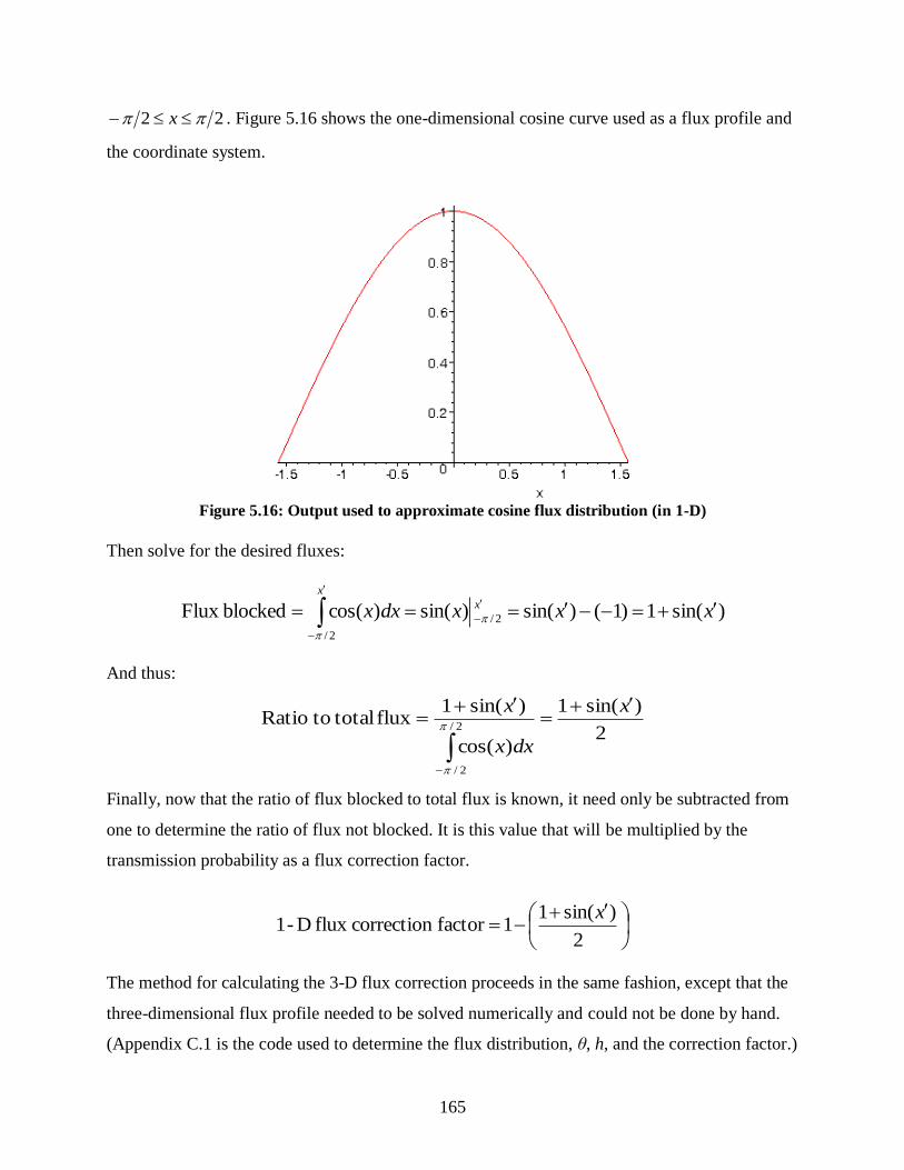
165
22 x . Figure 5.16 shows the one-dimensional cosine curve used as a flux profile and
the coordinate system.
Figure 5.16: Output used to approximate cosine flux distribution (in 1-D)
Then solve for the desired fluxes:
And thus:
2
)sin(1
)cos(
)sin(1flux total toRatio
2/
2/
x
dxx
x
Finally, now that the ratio of flux blocked to total flux is known, it need only be subtracted from
one to determine the ratio of flux not blocked. It is this value that will be multiplied by the
transmission probability as a flux correction factor.
The method for calculating the 3-D flux correction proceeds in the same fashion, except that the
three-dimensional flux profile needed to be solved numerically and could not be done by hand.
(Appendix C.1 is the code used to determine the flux distribution, θ, h, and the correction factor.)
)sin(1)1()sin()sin()cos(blockedFlux 2/
2/ xxxdxx
x
x
2
)sin(11factor correctionflux D-1
x

166
To calculate the three dimensional cosine distribution for a pipe, the value h was determined as
before to find the point in the cylindrical coordinate system at which the flux was being blocked.
A cosine distribution across the inlet of the cylindrical entrance region to the GV was assumed
once more; however, this time numerical integration was used to rotate this cosine curve around
the centerline (or z-axis) of this cylinder. Finally, only the portion corresponding to the gate
position (i.e. h) was considered to be blocked. These steps are illustrated in Figure 5.17.
Figure 5.17: 3-D representation of how 3-Dimensional flux was numerically integrated
The actual results for the total calculated flux are shown in Figure 5.18. Note that the reason that
parts of the curve appears to be ―cut-off‖ or cropped is because of the axes it is being plotted on
(in an x-y coordinate system) and because the z-axis was allowed to extend into negative values
(for the purposes of providing a better image).
Figure 5.19 shows the final results for the transmission probability (combined with the three-
dimensional flux correction) as a function of the effective GV diameter at a given GV position.
(By effective diameter, it is meant to say that it is the same dGV used earlier which assumed a
circular geometry. This was used once more for the purposes of being consistent with Equation
5.37. The use of dGV also allowed the axes to scale better, as compared to inlet area, and resulted
in a more legible plot.)
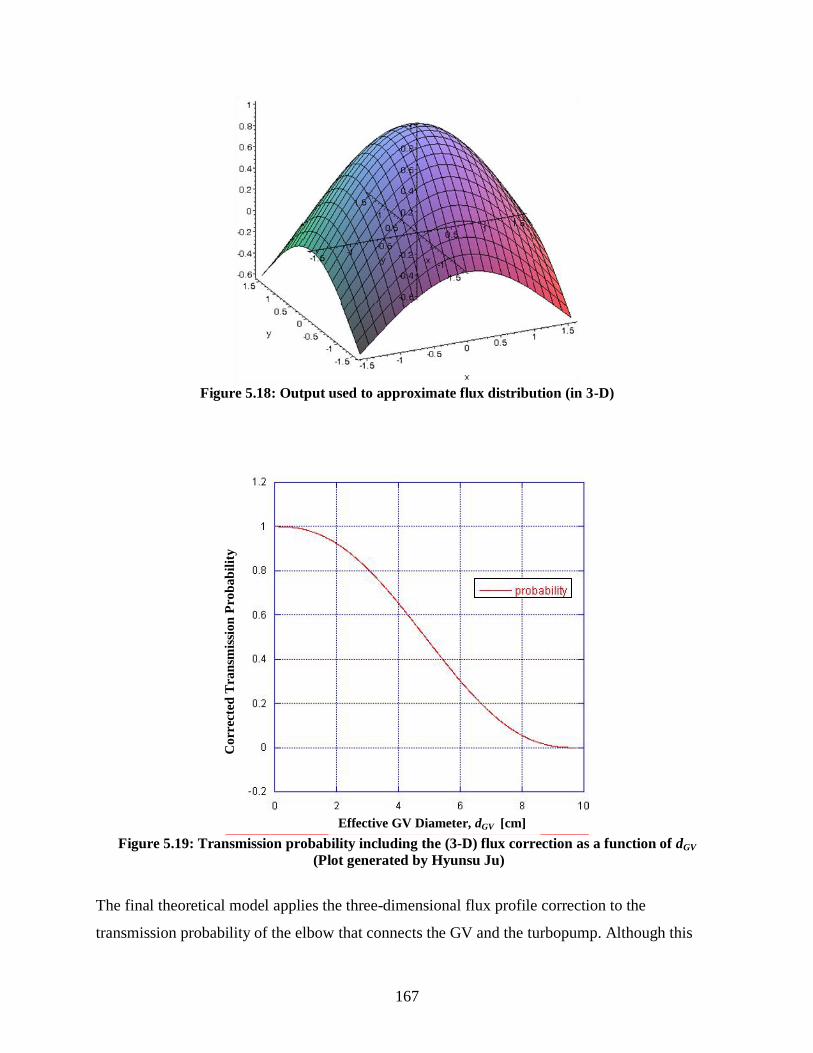
167
Figure 5.18: Output used to approximate flux distribution (in 3-D)
Figure 5.19: Transmission probability including the (3-D) flux correction as a function of dGV
(Plot generated by Hyunsu Ju)
The final theoretical model applies the three-dimensional flux profile correction to the
transmission probability of the elbow that connects the GV and the turbopump. Although this
Corr
ecte
d T
ran
smis
sion
Pro
bab
ilit
y
Effective GV Diameter, dGV [cm]

168
most likely exaggerates the drop in conductance due to the elbow by underreporting the elbow
transmission probability, the same argument for the initial flux correction can be made for the
elbow.
Namely, since the initial entrance to the elbow restricts the flux, the overall transmission
probability is effectively reduced because fewer particles reach the other end of the elbow
(because there are proportionally fewer particles available in the first place). In effect, this
eliminates the ―contraction between the GV and the elbow‖ (which was shown to have an almost
negligible impact on the conductance) and instead considers the elbow to have a reduced inlet
area. (Technically, this would no longer make the elbow a ―non-degenerate‖ elbow—or elbow of
constant diameter—for simplicities sake this will be ignored and the elbow will still be treated as
a straight pipe.)
The purpose of this final correction is merely to test the theory the other components
transmission probabilities may be an equally valid source of error. For example, the cross
adjacent to the GV would also have an effectively reduced transmission probability as a greater
number of particles reflect back into it after rebounding off of the GV gate. However, further
corrections were not investigated as at this point as the justifications, and associated math,
increasingly become more tenuous and the distinction between these correction factors and those
of experimentally-determined nature is blurred. The data for this final model will be briefly
discussed at the end of Chapter 6. All other models will be discussed in greater detail and will be
compared with experimental results.

169
CHAPTER 6
GAS DISTRIBUTION SYSTEM ANALYSIS
With the process of determining the various models already elaborated upon the results can be presented
in a concise format alongside the corresponding conclusions drawn from them. For the sake of clarity,
plots presented herein will only show the three major operating parameters considered (in terms of gas
flow rates). Each of the major models detailed in the previous chapter are shown although certain
variations of the models are excluded based on redundancy. The exceptions will be indicated and the
reasoning behind this will be fully explained as necessary. Additional plots can be found in the Appendix
where noted.
6.1 Experimental Models
Initial theoretical modeling of the gas distribution system began before the actual construction of the
system. Then, during the initial start-up period before system completion, data was gathered with regards
to the gas flow rates, set pressures, and gate valve positions. This data was not immediately used to
determine an experimental model. Instead a second theoretical model was created. Thereafter, variations
on the theoretical model and an experimental model were developed in conjunction. To facilitate the
comparison of these models the experimental model is presented first, followed by the theoretical models,
as opposed to presenting the models in chronological order of development.
6.1.1 Empirical Data and Limitations
The following data was recorded before the system design was finalized and construction
completed. The information shown in Table 6.1 was used to test the calibration of the two
capacitance manometers used to monitor actual system pressure. While the measurements were
being conducted the pressure values stabilized so rapidly during the gate valve adjustments that
no time-dependence could be determined. The only exceptions were in the rare circumstances in
which the gate valve was at the upper or lower bounds of its conductance and could not find a
stable position to maintain pressure and constantly adjusted position. Even in these
circumstances, pressure variation tended to be minor.
It was concluded that using Capacitance Manometer #2 provided accurate measurements for the
entire chamber even though it was attached to the reducing cross immediately before the gate

170
valve (GV). Additionally, minor fluctuations in pressure caused by gate valve adjustment were
not significant enough to cause a loop whereby the gate valve would have to continue correcting
repeatedly for pressure changes it induced.
CALIBRATION
(Multiply by 20 for units in mTorr)
CM #1 CM #2
0.911 0.905
0.875 0.876
0.845 0.846
0.801 0.802
0.710 0.712
0.623 0.625
0.484 0.487
0.375 0.379
0.301 0.305
0.223 0.228
0.178 0.183
0.087 0.086
0.000 0.000
Table 6.1: Comparison of Capacitance Manometers #1 and #2
The gas rates and pressures chosen for data analysis were based on bounds for the predicted
operating range of the system. During the course of initial film production, which was performed
after the completion of this research, it was determined and later confirmed in the literature that
such experimental models are only valid for a specific set of operating parameters and changing
one variable, such as geometry, can dramatically change system behavior. With this caveat in
mind it is important that the following results should only be considered in the context of a
system not actively engaged in film fabrication (or not configured for film fabrication—with
only an empty main chamber). Furthermore, it is uncommon to vary pressure during film growth
and exact gate valve position is irrelevant with respect to film growth as long as pressure is held
constant. In other words, a reproducible pressure is needed for reproducible film growth;
conductance and GV optimization are secondary concerns that can be examined once a final
operating pressure and gas-mixture ratio has been selected. This will represent a good area for
future work once the system has been finalized.

171
Figure 6.1: Initial pressure and gate valve readings taken with Capacitance Manometer #1
Figure 6.2: Initial pressure and gate valve readings taken with Capacitance Manometer #2

172
Relatively few data points were acquired during the initial conductance tests; as such the results
shown in Figures 6.1 and 6.2 should only be used as a general baseline for comparison. Items of
interest include the shape of curve and the upper and lower limits for a given flow rate. More
data points were not collected at the time of testing because the data was originally to be used to
determine the ―reliable‖ range of the GV. Ideally, it was planned that the GV would not operate
within 20% of either the upper or lower bounds (i.e. it would only be operated between 20-80%
open) so as to limit the uncertainty in GV position measurements. When measuring the position
few data points were taken as the point was not to use increasingly small increments for the
pressure at which the position was measured, but rather to use realistic integer value that might
be used for initial film growth tests.
Areas to note on the graph include: the steep front portion of the curve (or lower pressure limit),
the middle section or ―knee‖ of the curve (which may include the current operating range of 5
mTorr, depending on the flow rate) and the long tail end or ―plateau‖ that occurs at higher
pressure values. (20mTorr is the cut-off for our models and near the maximum pressure range
allowable for the turbopump.) The first plot, Figure 6.1, is based on readings from CM #1 which
is connected to the cluster flange attached to the left face of the primary chamber. Although the
strong correlation between CM #1 and #2 has been established, results in Figure 6.1 should not
be used as a direct source for comparison with the theoretical models. Instead a qualitative
comparison with the results for CM #2 will be provided.
Although it is not noted on the graph, setting the pressure lower than 2 mTorr and 4mTorr for
flow rates of 10 sccm and 20 sccm, respectively, forced the GV to go full open. (In more detail,
such settings caused it to fluctuate within a few percent of full open for several minutes without
reaching a stable position.) These lower pressure limits detected with CM #2 seem nearly
identical to those detected with CM #1.
It is important to note that GV position is only precise to three significant digits (i.e. the smallest
increment measureable is 0.1% or .001.)

173
Measurements conducted at 20 sccm ranging from 10 mTorr to 18 mTorr varied by less than
.005 (or 0.5% with respect to GV position, not one another) between CM #1 and #2. Results
deviated more at 10 sccm but were still close varying by 1-3% at points not at the upper limit of
GV position. Difference in the shape of the knee of the curves presented in Figures 6.1 and 6.2 is
simply due to the fact that more data points were acquired in this region using CM #2 than were
taken with CM #1. Finally it should be noted that there was some uncertainty as to whether the
final data point taken at 18 mTorr (at 10 sccm) with CM #1 was unstable and should have been
discounted.
Even though few data points were taken at 40 sccm they were sufficient to determine that the
system will not be operated with a 40 sccm gas flow rate (at least not in its current
configuration). Rather, film growth has most recently been conducted at a total pressure of 5
mTorr at a combined flow rate of Ar and O2 between 10 to 20 sccm (with Argon usually being
set at 10 sccm).
6.1.2 Experimental Fits
Based on the data presented in Table 5.1, the transmission probabilities for a tube of varying
length to diameter ratios, Eqn. 5.37 was developed. This is equation was based on a sigmoid
curve or ―S-curve.‖ This curve shape sees significant use in statistics and probabilistic risk
assessment as it physically represents the error function for a normal distribution and the
cumulative distributive function, respectively.
For the purposes of analyzing conductance subject to molecular flow, the idea of the cumulative
distribution function (or CDF) is important. A CDF is used to describe a given probability
distribution function (or PDF) in terms of one or more designated variables. This is pertinent
because the incoming flux of particles into a tube can be thought of as having a given
distribution or profile. A CDF of this distribution could then be used to determine the probability
of an individual particle (or variable) passing through the tube or being reflected back out. Based
on the shape of the curve, figures like Figure 5.19 are technically called complementary
cumulative distribution functions (or CCDFs) as they result from subtracting the values of the
CDF from 1.

174
The computer code provided in Appendix C.2 was developed by Hyunsu Ju and is used to
generate a CCDF or sigmoid curve fit for the input data using MATLAB. The input data consists
of the recorded pressures and GV position. The modified complementary logistics function used
to fit the data is provided below:
(6.1)
Where the m values are the six fitting coefficients to be determined using MATLAB. The results
for the 10 sccm and 20 sccm flow rates are presented in Tables 6.2 and 6.3. The fit was unable to
be performed on the 40 sccm data. (It is hypothesized that this is because there were simply not
enough data points available. However, it may also be possible that this particular model simply
won‘t extrapolate well to higher flow rates where viscous effects may have greater effect.
Further evidence to support this is the difference in shape between the 10 sccm and 20 sccm fits.)
10 SCCM FLOW RATE FITTING PARAMETERS
Coefficient Value 95% Confidence Interval
m1 18.00234 15.63309 20.3716
m2 38.03687 -2.8E+08 2.77E+08
m3 2.361974 -1.7E+07 17210944
m4 9.328447 -6.6E+07 66114256
m5 5.47194 -4654654 4654665
m6 0.400611 0.11423 0.686993
Table 6.2: Fit parameters for the 10 sccm flow rate experimental data
20 SCCM FLOW RATE FITTING PARAMETERS
Coefficient Value 95% Confidence Interval
m1 57.04402 -99.2657 213.3537
m2 41.83998 -2.9E+07 28622801
m3 0.781518 -534637 534638.3
m4 5.493562 -1.1E+07 11402886
m5 4.997004 -838396 838406
m6 0.381986 0.12056 0.643412
Table 6.3: Fit parameters for the 20 sccm flow rate experimental data
65 /)(
43
21 mmdV
GVemm
mmP

175
Based on the confidence intervals of the generated fit coefficients it would appear that 4 of the 6
coefficients have little impact on the final results. Therefore it is recommended for future work in
semi-empirical models that a simpler fit equation be used initially:
(6.2)
It is interesting to note that this more closely resembles the unmodified form of the
complementary logistics function given by:
Finally, one of the other downsides to this particular semi-empirical model is that it still employs
the ―effective GV diameter‖ dGV which needs to be calculated from Eqn. 5.38. The units of
centimeters were chosen over inches so as to better fit the graph to promote greater readability.
The results are presented in Figures 6.3 and 6.4 for flow rates of 10 and 20 sccm, respectively.
Figure 6.3: Experimental Model of Pressure vs. GV diameter at 10 sccm throughput
dGV [cm]
PV [
mT
orr
]
)/(121
1mdV
GVemP
xce
xF
1
11)(
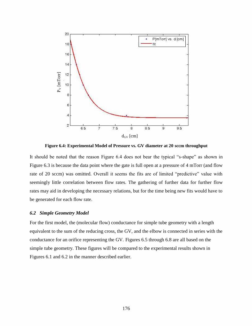
176
Figure 6.4: Experimental Model of Pressure vs. GV diameter at 20 sccm throughput
It should be noted that the reason Figure 6.4 does not bear the typical ―s-shape‖ as shown in
Figure 6.3 is because the data point where the gate is full open at a pressure of 4 mTorr (and flow
rate of 20 sccm) was omitted. Overall it seems the fits are of limited ―predictive‖ value with
seemingly little correlation between flow rates. The gathering of further data for further flow
rates may aid in developing the necessary relations, but for the time being new fits would have to
be generated for each flow rate.
6.2 Simple Geometry Model
For the first model, the (molecular flow) conductance for simple tube geometry with a length
equivalent to the sum of the reducing cross, the GV, and the elbow is connected in series with the
conductance for an orifice representing the GV. Figures 6.5 through 6.8 are all based on the
simple tube geometry. These figures will be compared to the experimental results shown in
Figures 6.1 and 6.2 in the manner described earlier.
dGV [cm]
PV [
mT
orr
]

177
Figure 6.5 was the original model produced (although the axes have been reversed since its
original production). Beginning at the far left, or lower controllable pressure limit, of each curve
as compared (i.e. for each flow rate) shows a good match between the experimentally determined
limits for 10 and 20 sccm and the predicted limits. The limit predicted for a flow rate of 40 sccm
was too high at 7.3 mTorr as compared to the experimentally determined value of approximately
6.2 mTorr. (Note: A flow of 5 sccm was not tested experimentally and thus no comparison will
be noted.) This indicates that the current model underestimates the conductance for a 40 sccm
flow when the GV is almost fully open. This would make sense as this is the situation furthest
from the molecular flow regime and where viscous effects would be most noticeable.
However, this trend does not apply to the middle or end of the flow rate curves. The predicted
GV position is far too low (i.e. the inlet area predicted is too small) for all flow rates measured
predicting the GV would be less than 5% open. This indicates the model conductance was set too
high.
Figure 6.5: Initial Pressure vs. GV position for simple tube geometry

178
6.2.1 Pump Speed Correction
A discretized correction was then applied as shown in Figures 6.6 and 6.8. This correction
incorporated the reduction in pump speed as the pressure was increased. The manner in which
the correction was implemented is discussed in detail in Chapter 5; suffice it to say the initial
(manually) discretized correction introduced the error associated with the discontinuities in the
curves. (This is most noticeable for the 40 sccm curve at the 8.5 mTorr mark.)
This correction slightly improves the curves by shifting the GV position higher (i.e. more open).
However, this correction only takes affect at the medium and high pressures seen in the knee and
tail region of each curve and only shifted them by a percent or two in the case of the 10 and 20
sccm flow rates. The effect was most noticeable in the knee of the 40 sccm curve near the 10
mTorr pressure mark. This information suggested the pump speed correction was of minimal
use, as originally predicted, but the decision was made to keep it in later versions of the models
for the sake of thoroughness.
Figure 6.6: Pressure vs. GV position for simple tube geometry with discretized correction for pump
speed reduction

179
6.2.2 Viscous Flow Corrections
In an early attempt to consider other models in addition to just the molecular conductance model,
different corrections were used to account for the viscous effects associated with gas flow in the
transition region. (This was discussed in further detail in Chapter 5.) The Knudsen correction
factor for transitional (or Knudsen) flow was applied to the conductance values per the method
detailed in Chapter 5. The results are shown in Figure 6.7.
Figure 6.7: Pressure vs. GV Position for simple tube geometry with Knudsen flow correction factor
Like for the pump speed correction, this correction also had the most noticeable effect on the
highest flow rate conductance curve. The 40 sccm curve was shifted to the left considerably so
that the low pressure limit matched the experimentally determined value. Unfortunately,
(although it is not very noticeable in the plots) it also shifted the 10 and 20 sccm curves a little
left thus making them less accurate and causing them to over predict the conductance.
Furthermore, for all flow rates, the middle and end portions of the curves were shifted further
down. (This was predicted considering that the viscous effects would increase the conductance of
the tubes.)

180
An alternate viscous correction was also used that considered the GV to be subject to molecular
flux (due to its restricted diameter) but treated the rest of the pumping stack according to laminar
viscous flow conditions. This correction also required manual discretization which introduced
errors into the results shown in Figure 6.8.
Like the values that used the Knudsen correction factor these curves also drop off more rapidly,
as compared to the experimental values, because they predict higher conductances than the
molecular model. However, it was not predicted that they would also shift all the curves to right
and, acting in reverse of previous corrections, have the minimal impact on the 40 sccm curve.
Due to the ad hoc nature of the implementation and the contradictory results, this approach was
deemed inappropriate and was not used further.
Figure 6.8: Pressure vs. GV Position for simple tube geometry with Knudsen flow correction factor
6.3 Complex Geometry Model
The basis for accounting for miscellaneous factors such as pump speed and viscous effects had
been suitably established. Subsequent corrections to the theoretical models then were focused on
tackling what was presumed to be the greatest source of error: the question of geometry.

181
The ―complex‖ geometry models accounts for the expansions and contractions of the
components (i.e. the pipes, GV and elbow) and their exact positions as they appear in series.
Initially it still treated the GV as an orifice with aGV = 1, but later models assumed the GV to be a
short tube of varying length to diameter ratio. (This was detailed in Chapter 5.) The results are
shown in Figures 6.9 and 6.10, respectively.
Unfortunately, comparison of Figures 6.9 and 6.5 (i.e. between the complex and simple tube
geometry models) reveals that the effects of the expansions and contractions alone are almost
negligible. Adding Figure 6.10 to the comparison shows that adjusting the transmission
probability of the GV has had the largest impact on results thus far. Still, this only provides a
slight but noticeable improvement of a few percent over the simple geometry model. The knee
and tail end values of the curve are still too small (in terms of GV opening) indicating the
conductance continues to be overestimated by the theoretical model as compared to the exact
results.
Figure 6.9: Pressure vs. GV Position for tubular geometry with expansions and contractions but
with the GV considered an orifice

182
Figure 6.10: Pressure vs. GV Position for tubular geometry with expansions and contractions and
with the GV considered a short tube
6.3.1 Pump speed Correction
An improved pump speed correction, shown in Figure 6.11, was applied in accordance with the
methodology established in Chapter 5. The results of the correction were virtually identical to
those applied to the simple tube geometry shown in Figure 6.6. Only the plot in which the
correction has been applied to the variable short tube GV is provided (because the short tube
correction provides more accurate results). (Exceptions will be made for situations where only
geometry is being dealt with exclusively.)
Compared to Figure 6.10 there is a slight shift up in curve position, and inversely a slight
decrease in the calculated conductance, but the results are still inadequate. Compared to the
experimental results, the shape of the flow rate curves may be recognizable but the actual
pressure values are of little use for predicting control system behavior.

183
Figure 6.11: Pressure vs. GV Position for tubular geometry with expansions and contractions and
with the GV considered a short tube. Pump speed reduction is accounted for.
6.3.2 Viscous Flow Correction
The Knudsen correction factor was now applied to the pump speed corrected values from Figure
6.11 in an attempt to look at the combined effect of all corrections. Once more the values for the
40 sccm are shifted to the left (effectively correcting the lower pressure limit). The overall
increase in conductance (or shift downward for GV values) with respect to the middle and end
portions of the curve is offset by the reduction in pump speed.
The application of the Knudsen correction to other variations of plots for the complex geometry
will not be shown. At this point, the Knudsen correction was assumed to only be pertinent at
higher flow rates and of little use for the newly determined operating gas flow range of between
10 and 20 sccm. Once more this suggests the gas flow present (at low pressures) can be
accurately represented by molecular flow. As such, the Knudsen correction will only be applied
to further models, when necessary, to facilitate comparison with earlier work for the sake of
thoroughness.

184
Figure 6.12: Pressure vs. GV Position for tubular geometry with expansions and contractions and
with the GV considered a short tube. Pump speed reduction and Knudsen flow are accounted for.
6.4 Flux Correction Models
The theoretical models were simply not conservative enough, despite a molecular flow based
model that, by definition, would be the most conservative model. Therefore it was posited that
there are other miscellaneous losses not accounted for. (This was already known to be true based
on the assumptions in Section 5.2 ergo the transmission probabilities are too large.) Figures 6.13
through 6.18 will now illustrate the final methodology applied to improve the conductance
calculations (as discussed in Chapter 5).
Both the one-dimensional and three-dimensional flux correction factors improve the results as
compared to the uncorrected complex geometry model. This is illustrated in two fashions: first,
by comparing Figures 6.9 and 6.13, and second, by comparing Figures 6.10 and 6.14. This was
done in stages to ensure that the effects of the flux correction could be distinguished from the
assumption of the GV as a short tube. This comparison shows that the flux correction alone
actually has a greater effect on the overall results than treating the GV as a short tube alone.

185
6.4.1 One-Dimensional Flux Correction Factor
Figure 6.13: Pressure vs. GV Position where expansions and contractions are accounted for but the
GV is considered an orifice subject to a one-dimensional cosine flux profile
Figure 6.14: Pressure vs. GV Position where expansions and contractions are accounted for and the
GV is considered a short tube subject to a one-dimensional cosine flux profile

186
However, the combination of the two corrections, as shown in Figure 6.14 still provides the best
results as compared to the experimental values. The positions of the values at the tail end of the
curves were shifted considerably higher. Changes were also noticed in the overall shape of the
curve. The size of the knee was more pronounced, indicating that there the rate at which the
conductance was changing in this region was decreasing (which would also explain why the tail
or plateau portion had shifted.) Interestingly enough, the lower limits of the curves were shifted
further left. (As usual this was most noticeable for the 40 sccm curve.) This correction improved
the 40 sccm results and seemed to have very little negative impact on the 10 and 20 sccm results
(certainly not enough to recommend removal of the correction).
The reason for this shift is that the flux correction supports there being a greater transmission
probability (and thus conductance) when the GV is near full open as compared to a geometry
where the circular area has simply been decreased linearly. This is because only one edge of the
(assumed) cosine flux profile is being blocked as opposed to the entire edge reason of the flux
profile all around the circumference of the GV. Conversely, once the GV has passed the half way
position and becomes nearer to being closed, the corrected flux profile suggests that a greater
number of particles have already been reflected predicting a lower transmission probability (and
conductance) than would be seen by a standard cosine flux profile directed at the center of a
small circular area. (This is because the cosine amplitude, or particle flux density, is greatest at
the center of the curve which coincides with the center of the pipe.)
Since the results of this model proved promising, it was then decided that a more accurate three-
dimensional model of the flux profile should be pursued. This is shown in Figure 6.15 and will
be discussed next.

187
6.4.2 Three-dimensional Flux Correction Factor
Figure 6.15: Pressure vs. GV Position with expansions and contractions accounted for and the GV
is considered a short tube subject to three-dimensional cosine flux profile
The difference between the one-dimensional and three-dimensional models is very slight, as seen
by comparing Figures 6.15 and 6.14. This is because in both cases the correction was based on
the ratio of flux blocked to total flux and the ratios for the one-dimension cosine curve and
(three-dimensional) rotated cosine curve are very similar except for when only the very edge of
the GV is blocked. This can be seen by noting the curves are shifted slightly further left near the
steep lower pressure portion of the curve, and by noting that the tail end of the curve is shifted
further up.
Again, corrections for pump speed reduction and Knudsen transitional flow were applied to both
one-dimensional and three-dimensional models. Due to their similarities, results of these
corrections are only shown for the three-dimensional model in Figures 6.16 and 6.17. The overall
changes to the plots, as compared to Figure 6.15, are the same as for previous applications of
these corrections and need not be discussed in further detail.

188
6.4.3 Pump Speed Correction
Figure 6.16: Pressure vs. GV Position with expansions, contractions, and pump speed reduction
accounted for and GV considered a short tube subject to three-dimensional cosine flux profile.
6.4.4 Viscous Flow Correction
Figure 6.17: Pressure vs. GV Position with expansions, contractions, pump speed reduction, and
Knudsen flow accounted for. GV considered short tube with three-dimensional cosine flux profile.

189
6.4.5 Additional Transmission Probability Correction
The final corrected model, shown in Figure 6.18, applies the three-dimension flux profile
correction factor to the transmission probability of the GV and to that of the elbow (which
connect the GV and the pump). (The pump speed reduction is also already included in this plot,
therefore plot Figure 6.18 should only be compared to Figure 6.16.) This had a noticeable impact
on the conductance curves, especially in the tail region of the curves, increasing them by roughly
2, 4, and 7 percent for the 10, 20, and 40 sccm flow rates, respectively. This final model should
be considered with more skepticism than the other models as the correction could just as easily
have been applied to the other components in the pumping stack; nevertheless, it does seem to
justify that these other transmission probabilities are in need of correction. This would be another
area of interest for future work in terms of gas conductance analysis.
Figure 6.18: Pressure vs. GV Position with expansions, contractions, and pump speed reduction
accounted for. GV (short tube) and elbow subject to three-dimensional cosine flux profile.

190
6.5 Conclusions
In terms of experimental results, further research needs to be conducted. However, knowing the
exact GV position is a secondary consideration and future semi-empirical models should focus
more on pressure than on GV position. It is important to note that, at this time, the semi-
empirical models need to be further refined before they can be extrapolated to other flow rates.
Other factors may also be included in addition to flow rate; these could include the location at
where the gas is introduced and the exact gas ratio/partial pressures for the gases introduced.
Unfortunately, none of the theoretical models were deemed adequate for providing a reliable
representation of the experimental results or for predicting later system operations. (Although
during more recent system operation the measured pressures and GV positions would
occasionally match those predicted by the models, this proved too inconsistent to be of any use.)
However certain conclusion can be made from the comparison of the various models.
First, corrections for viscous effects should only be used at higher flow rates. Second, the
reduction in pump speed due to increased pressure played a minimal role in terms of the overall
conductance but is still worth considering in all cases. Finally, these comparisons indicate that
there is a solid basis for using molecular flow based conductances to model the sputtering
system, but it is absolutely critical that the exact internal geometry be accounted for.
In further detail on this last point, the losses due to expansions and contractions in overall
diameter while passing from pipe to GV and back proved minimal. However, the actual effect of
the gate itself on transmission probability for all components of the system is absolutely critical.
If conductance optimization is to be performed, this will be a critical area for future research.
Finally, it was also proven that the actual flux profile of the incident particles impacting the gate
is also of significant interest (and the beaming effect of the reducing nipple and cross should be
investigated further as well).

191
CHAPTER 7
CONCLUSIONS
This thesis describes the scientific basis, the construction principles, and the operational
parameters of a system for the growth of thin, single crystal and polycrystalline films by means
of magnetron sputtering. In particular, this thesis deals with the design, construction, and
optimization of a magnetron sputtering system for urania deposition. The system will be used to
produce ceria and urania films with and without actinide surrogates that will then be irradiated at
high-temperature and used in several fuel characterization studies.
A magnetron sputtering system is an extremely complex system that requires extensive modeling
in order to be fully understood. It was the primary responsibility of the author to design, procure
the equipment for, and build the gas distribution system and its associated subsystems. The gas
injection and distribution system is a key component that relates to several variables involved in
the sputtering and film growth processes; therefore, it was also the responsibility of the author to
provide quantitative analysis on the behavior of the gas distribution system once it was
operational. Unfortunately, it is simply impossible to determine an analytical model to accurately
predict system behavior. This is caused by several factors but based on the previous analysis it
can be concluded that the most dominant effects are related to the relatively complex system
geometry with respect to transmission probability and to the necessity of operating within the
transitional flow regime. This conclusion is consistent with the findings of the literature on
vacuum technology and practices. Additional factors, such as change in turbomolecular pump
speed as a function of pressure and viscous effects, are less noticeable and in some cases
indeterminable.
Accurate experimental models can be produced and relate to existing curves that take the form of
complementary cumulative distribution functions (CCDFs) provided for varying transmission
probabilities. However, these logistical functions are purely statistical in nature, pertaining only
to the probability distribution of the gas particles passing through a tube under molecular flow
conditions; they do not capture the physics involved in molecular dynamics and thus are not

192
necessarily an adequate basis for extrapolation or interpolation. Additionally, the experimental
models generated are only valid for a specific set of operating parameters and changing one
variable can dramatically change system behavior. Once ideal operating parameters for film
growth have been established such semi-empirical models can be developed further.
With regards to the rest of the system, an overview of the design decisions and resulting
components selection is provided. The system design is included as well as more detailed
schematics for components built by the author, such as the power supply for the solenoid valves
(used to control the gas distribution valves and magnetron gun shutters). The ways in which
these components interact and help determine the film growth factors are explained by means of
Chapter 2 and 3. The literature surveyed has also provided a good basis for determining
operating parameters for urania and ceria film fabrication in Chapter 4. However, it is important
to note that these recommended parameters are configuration-specific and do not directly apply
to this sputtering system as they possess additional equipment not currently within the scope of
this system‘s design. Yet there is a general consensus about many other key operating parameters
that are directly relevant to its operation.
In brief, the conclusions are that the system should be maintained at as low a pressure as is
reasonably controllable. The substrate temperature should be set as high as is allowed. The
amount of reactive gas available should be just enough to ensure stoichiometric growth.
Energetic bombardment should be taken into account and controlled with a negative voltage bias
and low deposition rate. (One source suggested that only negative ions are a primary cause of re-
sputtering during reactive film deposition.) The angle-of-incidence should be kept as normal as
possible and gas scattering and thermalization should be avoided unless offset by bombardment.
There are conflicting recommendations with regards to geometry and where the process gases
should be introduced—no conclusion will be provided with regards to this. However, it is
recommended that tests be performed in directing a mix of oxygen and argon gas at the substrate
with varying gas ratios. As with the gas conductance analysis, determining ideal operating
parameters for all of these parameters will be an extremely complex process that requires
extensive experimentation.

193
In conclusion, the system is a functionally sound magnetron sputtering system for use in the
production of urania films, as well as other thin-films, under a wide variety of growing
conditions. Its robust and versatile feature set should allow for the fabrication of both epitaxial
and polycrystalline films with varying levels of actinide surrogates. The system provides a solid
foundation for future work and ultimately the objectives set forth in studying the ―Performance
of actinide-containing fuel matrices under extreme radiation and temperature environments.‖

194
CHAPTER 8
RECOMMENDATIONS FOR FUTURE WORK
The magnetron sputtering system will be involved in numerous projects as it will be one of the
only sources of uranium-based films for university research. This section will only detail future
work that can be readily pursued with regards to system design and modeling.
8.1 Recommendations for Gas Conductance Modeling
Gas modeling can continue to be developed exclusively or as part of an overall modeling effort
for system behavior with regards to film growth. If the former course is pursued, the work
presented herein can be expanded upon by performing Monte Carlo calculations. This numerical
method could initially be used to study molecular flow for the exact geometry of the system.
Later, more advanced molecular dynamics simulations could be used to account for a host of
processes affecting gas kinetics.
Analytical methods have proven to be of limited use but further physical insights may be gained
by estimating and then correcting for losses due to complex geometry within the current model.
In order to do this, a few important assumptions must be addressed. The first suggested area for
further study involves the flux profile and the change in shape as it proceeds down the length of
the tube. A simple modification of the proposed cosine distribution could adjust the amplitude
and width of the curve as a function of the ratio of tube length to diameter. The correction term
used would most likely need to be based on empirical results similar to those shown in
O‘Hanlon. The next suggested area for improvement corresponds to accounting for
miscellaneous decreases in conductance.
Previously mentioned regions which reduce conductance but were assumed to be negligible
include volumes such as the small ports on the reducing cross and slit-like areas along the edges
of the gate valve. These factors will all reduce the transmission probability of particles which
enter the pumping stack; however, it is theorized that the effect of the GV gate itself will still be
the most significant reducing factor. Again, Monte Carlo methods would be best suited to this

195
task, but only examining select areas as opposed to the entire system would greatly reduce the
complexity of the Monte Carlo simulation required. These could then be considered precursors to
the proposed full Monte Carlo simulation and may predict whether such an undertaking is
worthwhile. Finally, the pump speed can be measured experimentally and then combined in
series with the conductances using the Oatley and Haefer Method (as described in Chapter 5).
This will eliminate all the known geometry-associated sources of error in the theoretical models.
(Error due to viscous effects in the transition region still will not be accounted for.)
Alternatively, a semi-empirical model could be used if an additional pressure gauge was used to
determine the pressure drop across the gate valve. This would allow the conductance to be
determined based on a continuum flow model. The continuum model could then be combined
with the molecular flow based model using Knudsen‘s method for calculating transition
conductance. This would better incorporate viscous effects in the existing model than the current
method of a pressure based correction factor by eliminating the need for a round of iteration.
Again, it is recommended that these types of corrections only be applied to higher flow rate
scenarios and not to the currently used operating parameters for film growth.
8.2 Recommendations for System Design
Future work with regards to overall system design could begin with simply rearranging the
components of the current configuration so as to optimize performance. Previously considered
components, that were not initially deemed to be of significant cost/benefit ratio, may also be
introduced. The order of construction and implementation should correspond to the relative
degree of importance in the system architecture and relative cost.
A more costly component called for in the original design, but which is now optional, is the
liquid nitrogen cold trap. The cold trap would increase the purity of the system by effectively
removing condensable impurities that may outgas during regular operation. The most common
impurity this process would remove is water vapor. The degree to which this ultimately affects
the vacuum is primarily dependent on the ratio of impurities being deposited into the chamber
(by outgassing, leaking, etc.) and the surface area available to condense upon. The available
room for a cold trap, and thus the size and effectiveness of the cold trap, is constrained by the

196
fact it needs to be located near the bottom of the chamber and near the magnetron guns. One
recommendation to account for some of these obstacles is the use of (manufacturer cleaned)
VCR tubing with a braided sheath. This option bears further investigation if system purity (and
the ultimate pressure) is to be increased in the future. Benefits to simply increasing the system
conductance include lowering the ultimate pressure attainable (and thereby increasing system
purity) by increasing the effective pumping speed. This may not have as significant an impact as
a cold trap and may be significantly more costly, but it would also drastically decrease pump
down time (which is a matter of convenience).
Steps to increase system conductance would involve drastic changes to the pumping stack design
and/or pump replacement. Yet it is important to note that installation of a larger (or higher
capacity) turbomolecular pump to the pumping stack as is would have a minimal effect on the
effective pumping speed. This is because the GV and the associated pipework (that compose the
pumping stack) are currently the limiting factors with respect to gas conductance. Larger
diameter pipework would increase conductance, but given the current GV its effect would also
be limited. Rather, shortening the length of (tubing used for) the pumping stack would have the
greatest affect at the lowest cost.
One such option would be the removal of the elbow; yet this would result in the pump being
exposed to more particulates thus potentially decreasing the pump life. Alternatively (or
additionally), the cross could be removed if the Baratron gauge was relocated elsewhere. (One
location would be the top of the sample stage, this would allow for a more local pressure reading
as with respect to substrate location, but again this may result in the exposure of the Baratron and
thus a reduced lifetime.) No clear recommendation can be made with regards to increasing gas
conductance out of the main chamber. Yet if the 6-inch TMP 351 were to be replaced, it could
then be used on the load-lock in place of the TMP 150. Since the TMP 351 has the same
diameter as the load-lock it would have a significant impact on the pump down time of the load-
lock. This is especially important as the current design of the load-lock requires considerable
pump down time due to the constricted volume to be evacuated present within the sample
transfer arm.

197
Finally, there are some recommendations pertinent to the film growth capabilities of the system.
The inclusion of a RHEED system and enhanced substrate heater are highly recommended for
increased functionality. The ability to characterize films while in the process of growing them
may aid in determining optimal operating parameters in real-time. This would also aid in future
work in film growth optimization. This feature would be of even greater benefit when co-
sputtering materials in order to make compound films with a pre-determined ratio. It has also
been suggested that a change in substrate heater may aid in producing epitaxial films via
magnetron sputtering. The upgraded heater would have to be able to reach temperatures near the
melting point of the desired oxide. For the purposes of forming urania this may prove impossible
as the melting point of urania is significantly higher than Inconel. In addition to an alternate
sample holder, such a heater would most likely necessitate a cooling jacket be applied to the
exterior of the primary chamber. A preliminary search has also indicated that the upper limit of
non-custom substrate heaters for use in an oxygen rich environment appears to be in the range of
1000-1200°C. At this time both of these features would be considered luxuries and are not
necessary for high quality film production. (Further study is required to ascertain whether the
increase in substrate heating is worth the financial and design costs involved.) However there are
some other less costly enhancements that would increase film quality.
Features that would allow the use of a RF plasma in conjunction with a DC plasma or as a means
of ionizing the reactive gas or target material would aid in film growth. The degree of
complexity involved varies by location and the feature to be used. The simplest design would
merely require a RF coil be applied around the (optional) O2 feed through. More involved
additions, such as an electron source, require further investigation with regards to cost and
design. As such these features should only be considered a preliminary recommendation.
Despite these design suggestions, the system is already a fully-operational and capable
magnetron sputtering system. It is an essential tool for nuclear fuel characterization and general
materials research. The system itself also provides for several avenues of further research not
necessarily related to the films it is used to fabricate. Extensive modeling and an evolving design
will ensure that it remains a vital resource throughout its long lifetime.

198
REFERENCES
[1] Heuser, B. (2007). Project Narrative: A Nuclear Engineering Research Initiative for
Consortia (NERI-C) for the Performance of actinide-containing fuel matrices under extreme
radiation and temperature environments. ts. NPRE Dept. UIUC, Urbana.
[2] Mattox, D. (1998). Handbook of Physical Vapor Deposition (PVD) Processing: Film
Formation, Adhesion, Surface Preparation and Contamination Control. Park Ridge, New Jersey:
Noyes Publications. 4,209-210,330-333,230-233,326-327,315-324,468-488,338-343,444-450,
471 ,242,111,47-55.
[3] O‘Hanlon, J. (2003). A user’s guide to vacuum technology. Hoboken, New Jersey: John
Wiley and Sons, Inc. 4,9-23,25-52,58,126-130,201-204,209-211,217-225,467,469-472,274.
[4] Smith, D. (1995). Thin-Film Deposition: Principles and Practice. Boston, Massachusetts:
McGraw-Hill. 483.
[5] Thorton, J. (1986). The Microstructure of Sputter-deposited Coatings. Journal of Vacuum
Science Technology, A4(6), 3059-3065.
[6] Berg, S. & Nyberg, T. (2005). Fundamental understanding and modeling of reactive
sputtering processes. Thin Solid Films, 476, 215-219.
[7] Savvides, N., Thorley, A., Gnanarajan, S. & Katsaros, A. (2001). Epitaxial growth of
cerium oxide thin film buffer layers deposited by d.c. magnetron sputtering. Thin Solid Films,
388, 177-182.
[8] International Nuclear Safety Center. Summary –density of solid uranium dioxide. Retrieved
September 10, 2009 from http://www.insc.anl.gov/matprop/uo2/density/solid/soldens.php.
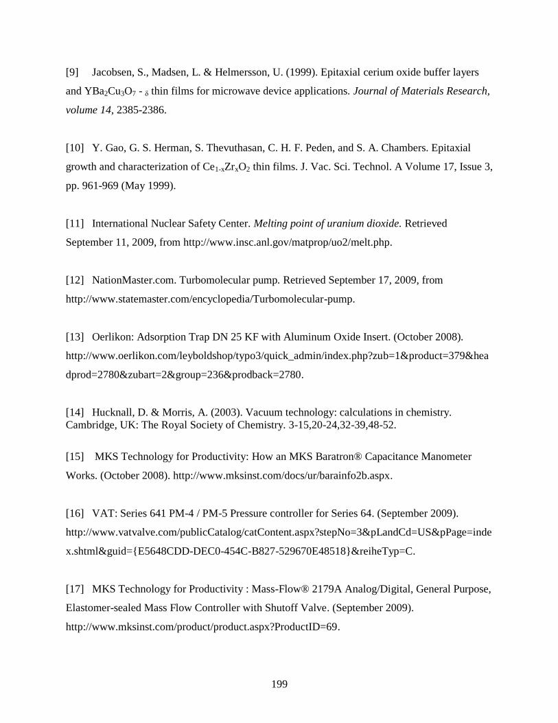
199
[9] Jacobsen, S., Madsen, L. & Helmersson, U. (1999). Epitaxial cerium oxide buffer layers
and YBa2Cu3O7 - δ thin films for microwave device applications. Journal of Materials Research,
volume 14, 2385-2386.
[10] Y. Gao, G. S. Herman, S. Thevuthasan, C. H. F. Peden, and S. A. Chambers. Epitaxial
growth and characterization of Ce1-xZrxO2 thin films. J. Vac. Sci. Technol. A Volume 17, Issue 3,
pp. 961-969 (May 1999).
[11] International Nuclear Safety Center. Melting point of uranium dioxide. Retrieved
September 11, 2009, from http://www.insc.anl.gov/matprop/uo2/melt.php.
[12] NationMaster.com. Turbomolecular pump. Retrieved September 17, 2009, from
http://www.statemaster.com/encyclopedia/Turbomolecular-pump.
[13] Oerlikon: Adsorption Trap DN 25 KF with Aluminum Oxide Insert. (October 2008).
http://www.oerlikon.com/leyboldshop/typo3/quick_admin/index.php?zub=1&product=379&hea
dprod=2780&zubart=2&group=236&prodback=2780.
[14] Hucknall, D. & Morris, A. (2003). Vacuum technology: calculations in chemistry.
Cambridge, UK: The Royal Society of Chemistry. 3-15,20-24,32-39,48-52.
[15] MKS Technology for Productivity: How an MKS Baratron® Capacitance Manometer
Works. (October 2008). http://www.mksinst.com/docs/ur/barainfo2b.aspx.
[16] VAT: Series 641 PM-4 / PM-5 Pressure controller for Series 64. (September 2009).
http://www.vatvalve.com/publicCatalog/catContent.aspx?stepNo=3&pLandCd=US&pPage=inde
x.shtml&guid={E5648CDD-DEC0-454C-B827-529670E48518}&reiheTyp=C.
[17] MKS Technology for Productivity : Mass-Flow® 2179A Analog/Digital, General Purpose,
Elastomer-sealed Mass Flow Controller with Shutoff Valve. (September 2009).
http://www.mksinst.com/product/product.aspx?ProductID=69.

200
[18] MKS Technology for Productivity: 247D Four Channel Power Supply/Readout.
(September 2009). http://www.mksinst.com/product/product.aspx?ProductID=85.
[19] Inoue, T. Shida, S. & Kato, K. (2006). Oxygen radical irradiation effect in reactive
magnetron sputtering for orientation selective epitaxial growth of CeO2(100) layers on Si(100)
substrates. Journal of Crystal Growth, 289, 534-539.
[20] Inoue, T., Sakamoto, N, Ohashi, M. Shida, S. & Horikawa, A. (2004). Orientation selective
epitaxial growth of CeO2 (100) and CeO2 (110) layers on Si (100) substrates. Journal of Vacuum
Science Technology, A 22, 46-48.
[21] Inoue, T., Ohashi, M., Sakamoto, N. & Shida, S. (2004). Orientation selective epitaxial
growth of CeO2 layers on Si(100) substrates using reactive DC magnetron sputtering with
substrate bias. Journal of Crystal Growth, 271, 176-183.
[22] Hollmann, E., Zaitserv, A., Loginov, E., & Likholetov, Y. (1992). Rapid communication:
CeO2 films deposited by DC reactive magnetron sputtering. Journal of Physics D : Applied
Physics, 25, 504-505.
[23] Miserque, F., Gouder, T., Wegen, D. & Bottomley, P. (2001). Use of UO2 films for
electrochemical studies. Journal of Nuclear Materials, 298, 280-290.
[24] Rogers, M. (1965). Mass transport and grain growth induced by fission fragments in thin
films of uranium dioxide. .Journal of Nuclear Materials, 16, 298-305
[25] Van den Berghe, S., Miserque, F., Gouder, T., Gaudreau, B. & Verwerft, M. (2001). X-ray
photoelectron spectroscopy on uranium oxides: a comparison between bulk and thin layers.
Journal of Nuclear Materials, 294, 168-174.
[26] King, R., Senanayake, S., Chong, S. & Idriss, H. (2007). The reactions of acetone with the
surfaces of uranium dioxide single crystal and thin film. Surface Science, 601, 5690-5700.

201
[27] Danielson, P. (March 1999). Creating a Vacuum. Retrieved November 4, 2008, from
http://www.vacuumlab.com.
[28] Shinagawa, H., Setyawan, H., Asai, T., Sugiyama, Y. & Okuyama, K. (2002). An
experimental and theoretical investigation of rarefied gas flow through circular tube of finite
length. Chemical Engineering Science, 57, 4027-4036.
[29] Weisstein, E.W. Circular Segment retrieved from MathWorld- a Wolfram web resource.
Retrieved November 18, 2008, from http://mathworld.wolfram.com/CircularSegment.html.
[30] Ask Dr. Math ®. 1994-2010. Drexel University web resource. Retrieved November 18,
2008, from http://mathforum.org/dr.math/faq/faq.circle.segment.html.
All pictures courtesy of Hyunsu Ju, Eric Reside, Susan Mumm, and Robert Gennardo.

202
APPENDIX A: ADDITIONAL FIGURES AND TABLES
A.1 Additional Photos
Figure A.1: The heating tape being applied in order to bake out the main vacuum chamber
Figure A.2: Chamber wrapped in heating tape and aluminum foil. Heating tape is shown connected
to the Variac transformer used to adjust the voltage supplied to the tape.

203
Figure A.3: Sample holder after being heated to 850°C in main chamber

204
Figure A.4: Water manifold with secondary and tertiary valves (under construction)
Figure A.5: View of the system from behind the load-lock

205
A.2 Alternate Plots (Reversed axes)
Figure A.6: Pressure vs. GV Position for complex geometry
Figure A.7: Pressure vs. GV Position for complex geometry with GV treated as orifice subject to
one-dimensional cosine flux profile

206
Figure A.8: Pressure vs. GV Position for complex geometry with GV treated as short tube subject
to one-dimensional cosine flux profile
Figure A.9: Pressure vs. GV Position for complex geometry with GV treated as orifice subject to
three-dimensional cosine flux profile

207
Figure A.10: Pressure vs. GV Position for complex geometry with GV treated as short tube subject
to three-dimensional cosine flux profile
Figure A.11: Pressure vs. GV Position for complex geometry with GV treated as orifice subject to
three-dimensional cosine flux profile. Pump speed reduction has been accounted for.

208
Figure A.12: Pressure vs. GV Position for complex geometry with GV treated as short tube subject
to three-dimensional cosine flux profile. Pump speed reduction has been accounted for.
Figure A.13: Pressure vs. GV Position for complex geometry with GV treated as orifice subject to
three-dimensional cosine flux profile. Pump speed reduction and Knudsen flow are accounted for.

209
Figure A.14: Pressure vs. GV Position for complex geometry with GV treated as short tube subject
to three-dimensional cosine flux profile. Pump speed reduction and Knudsen flow accounted for.
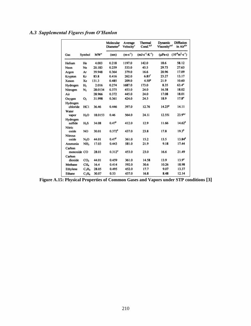
210
A.3 Supplemental Figures from O’Hanlon
Figure A.15: Physical Properties of Common Gases and Vapors under STP conditions [3]

211
APPENDIX B: MATERIALS PROVIDED BY DR. HEUSER
B.1 Initiation and Termination Procedures
SOP 1—Initiation of primary chamber pumping system.
1. Confirm primary chamber gate valve (GV1), load lock gate valve (GV2), Ar vent valve
into primary turbo pump (VV1) and load-lock turbo pump (VV2), foreline valve to
primary turbo pump (FV1), and foreline valve to load-lock turbo pump (FV2) are all
closed.
2. Confirm Ar and O2 mass flow valves are closed.
3. Confirm that the GV1 control box is on. Confirm that the primary turbo pump control
box is on.
4. Confirm the convectron gauge connected to the primary chamber (CG1) is on and
recording pressure.
5. Start mechanical pump wait 1-2 minutes for pump to war.
6. Open FV1 and wait until ―gurgling‖ sound in mechanical pump stops. If gurgling sound
does not stop within 1-2 minutes close FV1 and turn off mechanical pump. Abort
attempt.
7. Immediate after gurgling sound stops, push Set Point 1 button on the GV1 control box
and then push ―Position Mode‖ button. This opens GV1 to the 5% open position.
Mechanical pump should gurgle again, assuming the primary chamber was backfilled
with Ar. If not, mechanical pump may not gurgle. CG1 should exhibit rapid reduction in
primary chamber pressure. If not, immediately close GV1 by pushing the ―Close‖ button
on the control box. Once rapid pressure reduction is confirmed, fully open GV1 by
pushing the ―Open‖ button on the control box.
8. Immediately after the CG1 pressure falls below 10-1
Torr, start the primary turbo pump
coolant (confirm coolant flow) and push the ―Start‖ button on the primary turbo pump
control box. Confirm that the load on the primary turbo pump increases and then
decreases to one (1) light on the turbo pump control box. This should take at most a few
minutes. If the load on the turbo pump increases but then does not begin to decrease,
immediately close GV1 by pushing the ―Close‖ button on the control box. Monitor load
on the primary turbo pump—if it does not fall to 1 light, turn off turbo pump and follow
SOP 3.
9. After a few minutes attempt to start the ion gauge connected to the primary chamber
(IG1). Depending on the recent activity in the primary chamber, the pressure reading
should be in the low 10-5
to 10-6
Torr range and falling.

212
SOP 2—Termination of primary chamber pumping system.
1. Confirm that the 1000-Torr Baratron Gauge (CM3) is on and recording approximately
zero pressure. If CM3 is not working properly, close the primary chamber gate valve
(GV1) and follow SOP3.
2. If CM3 is working properly and reading zero pressure, confirm GV1 is open. If GV1 is
closed and cannot be opened (for example, because of high primary chamber pressure),
follow SOP 3.
3. Close window shutter on the primary chamber.
4. Confirm that the foreline valve to load-lock turbo pump (FV2) is closed and that the load-
lock turbo pump is off. IF NOT, SKIP STEP 8 BELOW AND PERFORM STEP 7A.
5. Open low purity or vent Ar bottle and set low pressure side of the regulator to a
maximum of 5 psig (5 psi above 1 atm.). Note that the ―zero‖ reading of the low pressure
side of the vent Ar regulator is 1 atmosphere. Open the small valve from the regulator to
the Ar vent line. DO NOT open vent line to the primary turbo pump (VV1).
6. Push the ―Stop‖ button on the primary turbo pump control box and turn off the primary
turbo pump coolant.
7A. SKIP THIS STEP unless FV2 is open and load-lock turbo pump is running. Close
the primary turbo pump foreline valve (FV1).
7. Open VV1.
8. SKIP THIS STEP if FV2 is open and load lock turbo pump is running. Turn off
the mechanical pump immediately after opening VV1.
9. Confirm Ar flow into the primary chamber by monitoring the chamber pressure with
CM3. NOTE: The CG1 reading is gas specific and calibrated for air. It will not record
760 Torr (1atm.) for Ar and should be ignored during venting.
10. When CM3 reaches approximately 100 Torr close the primary gate valve (GV1) by
pushing the ―Close‖ button on the control box. Do not go above 100 Torr on CM3
without permission from Prof. Heuser. If CM3 reaches a plateau pressure significantly
below 100 Torr move to Step 11 or readjust regulator to 5 psig.
11. Close VV1.
12. In the following order, close FV1, close small valve from the regulator to the Ar vent
line, close the regulator and close the vent Ar bottle.

213
SOP 3—Termination of primary chamber pumping system with primary
gate valve closed.
NOTE: THIS SOP FOLLOWED ONLY IF PRIMARY CHAMBER GATE VALVE GV1 IS
CLOSED AND CANNOT BE OPENED.
1. Confirm that the foreline valve to the load-lock turbo pump (FV2) is closed and that the
load-lock turbo pump is off. IF NOT, SKIP STEP 5 AND PERFORM STEP 3A.
2. Open low purity or vent Ar bottle and set low pressure side of the regulator to a
maximum of 5 psig (5 psi above 1 atm.). Note that the ―zero‖ reading of the low pressure
side of the vent Ar regulator is 1 atmosphere. Open the small valve from the regulator to
the Ar vent line. DO NOT open vent line to the primary turbo pump (VV1).
3A. SKIP THIS STEP unless FV2 is open and load lock turbo pump is running. Close
the primary turbo pump foreline valve (FV1).
3. Push the ―Stop‖ button on the primary turbo pump control box and turn off the primary
turbo pump coolant.
4. Open VV1.
5. SKIP THIS STEP if FV2 is open and load lock turbo pump is running. Turn off
the mechanical pump immediately after opening VV1.
6. Confirm that the primary chamber turbo pump has stop rotating by listening for
termination of whinnying sound. At most, wait 2 minutes before performing Step 7.
7. Immediately in the following order, close VV1, close small valve from the regulator to
the Ar vent line, close the regulator and close the vent Ar bottle.

214
B.2 System Schematic
Fig
ure
B.1
: O
rig
ina
l S
yst
em S
chem
ati
c (H
ard
cop
y p
rov
ided
by
Pro
fess
or
Heu
ser;
rec
rea
ted
in
Pow
erP
oin
t b
y a
uth
or)

215
APPENDIX C: COMPUTER CODE PROVIDED BY HYUNSU JU
C.1 Cosine Distribution and Correction Output
clear all;
total_v=0;
dx=0.001;
for x=-pi/2+dx:dx:pi/2-dx
range=sqrt((pi/2)^2-(abs(x))^2);
y=-range:0.001:range;
z=cos(sqrt(x^2+y.^2));
total_v=total_v+trapz(y,z)*0.001;
end
total_v
H=xlsread('h.xls');
D=3.834*2.54;
h=pi*H/D-pi/2;
num=1001;
vol=zeros(1001,1);
for i=1:num
xo=h(i);
for x=xo:dx:pi/2
range=sqrt((pi/2)^2-(abs(x))^2);
if range > 0
y=-range:0.001:range;
z=cos(sqrt(x^2+y.^2));
vol(i,1)=vol(i,1)+trapz(y,z)*0.001;
end
end
end
result=vol/total_v;
title={'H [cm]','probability'};
xlswrite('cosine_dist.xls',title,'Sheet1','A1');
xlswrite('cosine_dist.xls',H,'Sheet1','A2');
xlswrite('cosine_dist.xls',result,'Sheet1','B2');

216
clear all;
GV=[0.001:0.001:0.999]';
R=3.834/2*2.54; %[cm]
k=2*pi*(1-GV);
n=5000000; % max. iteration num.
tmp=(6*k).^(1/3);
x=tmp-(tmp-sin(tmp)-k)./(1-cos(tmp));
err = 0.000001*ones(999,1); % error
count=0;
for i=1:n
tmp=x;
x=x-(x-sin(x)-k)./(1-cos(x));
count=count+1;
if abs(x-tmp) < err
%disp('TRUE,Dave!')
sol=x;
count
break;
end
end
title={'GV','sol','H [cm]','correction'};
H=R*(1-cos(sol/2));
CR=1-(sin(H/2/R*pi-pi/2)+1)/2;
xlswrite('iter_theta.xls',title,'Sheet1','A1');
xlswrite('iter_theta.xls',sol,'Sheet1','B2');
xlswrite('iter_theta.xls',GV,'Sheet1','A2');
xlswrite('iter_theta.xls',H,'Sheet1','C2');
xlswrite('iter_theta.xls',CR,'Sheet1','D2');
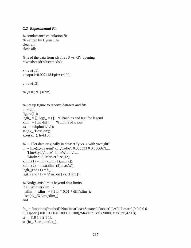
217
C.2 Experimental Fit
% conductance calculation fit
% written by Hyunsu Ju
clear all;
close all;
% read the data from xls file ; P vs. GV opening
raw=xlsread('40sccm.xls');
x=raw(:,1);
x=sqrt(4*0.0074484/pi*x)*100;
y=raw(:,2);
%Q=10; % [sccm]
% Set up figure to receive datasets and fits
f_ = clf;
figure(f_);
legh_ = []; legt_ = {}; % handles and text for legend
xlim_ = [Inf -Inf]; % limits of x axis
ax_ = subplot(1,1,1);
set(ax_,'Box','on');
axes(ax_); hold on;
% --- Plot data originally in dataset "y vs. x with yweight"
h_ = line(x,y,'Parent',ax_,'Color',[0.333333 0 0.666667],...
'LineStyle','none', 'LineWidth',1,...
'Marker','.', 'MarkerSize',12);
xlim_(1) = min(xlim_(1),min(x));
xlim_(2) = max(xlim_(2),max(x));
legh_(end+1) = h_;
legt_{end+1} = 'P[mTorr] vs. d [cm]';
% Nudge axis limits beyond data limits
if all(isfinite(xlim_))
xlim_ = xlim_ + [-1 1] * 0.01 * diff(xlim_);
set(ax_,'XLim',xlim_)
end
fo_ = fitoptions('method','NonlinearLeastSquares','Robust','LAR','Lower',[0 0 0 0 0
0],'Upper',[100 100 100 100 100 100],'MaxFunEvals',9000,'MaxIter',4200);
st_ = [18 1 3 2 1 1];
set(fo_,'Startpoint',st_);

218
ft_ = fittype('m1-m2/(m3+m4*exp(-(x-m5)/m6))' ,...
'dependent',{'y'},'independent',{'x'},...
'coefficients',{'m1', 'm2', 'm3', 'm4','m5','m6'});
% Fit this model using new data
cf_ = fit(x,y,ft_ ,fo_);
% Plot this fit
h_ = plot(cf_,'fit',0.95);
legend off; % turn off legend from plot method call
set(h_(1),'Color',[1 0 0],...
'LineStyle','-', 'LineWidth',2,...
'Marker','none', 'MarkerSize',6);
legh_(end+1) = h_(1);
legt_{end+1} = 'fit';
hold off;
legend(ax_,legh_, legt_);
% save the coefficients resulting from fit
fitcoeff=coeffvalues(cf_);
fitconfint=confint(cf_,0.95);
fitconfint
cf_
% Now define the title to be saved with the data in the Excel file
title={'fit coeff.','values','95% confidence'};
coeff={'m1', 'm2', 'm3', 'm4','m5', 'm6'};
xlswrite('final_fit.xls',title,'Sheet1','A1');
xlswrite('final_fit.xls',coeff','Sheet1','A2');
xlswrite('final_fit.xls',fitcoeff','Sheet1','B2');
xlswrite('final_fit.xls',fitconfint','Sheet1','C2');
%xlswrite('final_fit_coeff.xls',fitcoeff','Sheet1','A1');
% save the fit result
yfit=feval(cf_,x);
fittitle={'x','y','yfit'};
xlswrite('fit_result.xls',fittitle,'Sheet1','A1');
xlswrite('fit_result.xls',x,'Sheet1','A2');
xlswrite('fit_result.xls',y,'Sheet1','B2');
xlswrite('fit_result.xls',yfit,'Sheet1','C2');

219
AUTHOR’S BIOGRAPHY
David Joseph Gennardo was born in Oak Park, IL on April 19, 1984. Due to his parents and
some exceptional instructors he was instilled with a sense of wonder and passion for the
sciences, history and literature at a young age. After a varied and somewhat tumultuous
undergraduate career (in which he went through four different majors) he had the good fortune to
stumble upon the Nuclear, Plasma, and Radiological Engineering Department at Illinois. It was
there he met a wonderful group of educators and peers who shared his interests and were just
generally agreeable. After five years with the department it has become more a surrogate family
than an institution.
He graduated from the University of Illinois at Urbana-Champaign with a Bachelor of Science in
May 2007 and will be completing his Masters Degree in 2010. As a graduate research assistant
he had the opportunity to help design, construct and operate a (rather impressive) magnetron
sputtering system. He was inducted into Alpha Nu Sigma in the spring of 2009 and has had the
honor of representing his fellow students as a representative for the Nuclear Engineering Student
Delegation in 2008 and 2009. He currently works as a Nuclear Associate at Sargent & Lundy in
Chicago, IL in the Nuclear Technology and Regulations Group.
As he continues on with his life David is confident that he will continue to advocate for the
benefits of nuclear power as part of a reasonable energy policy, continue to strive for self-
improvement and continue to enjoy taking walks in the rain.
He has an interesting sense of humor.