design and reliability-based optimization of the
TRANSCRIPT

1
Design and Reliability-based
Optimization of the Piezoelectric Flex
Transducer
By
Liheng Luo
Thesis submitted for the degree of Doctor of Philosophy
at Lancaster University
Submitted
March, 2018

2
ACKNOWLEDGEMENTS
To begin with I would like to express my gratitude to those who have supported me
over the last four years whilst conducting this research. First of all, I would like to
express my deepest gratitude to my Supervisor, Prof Jianqiao Ye, for giving me the
opportunity to do this PhD and for sharing his great ideas with me. I would also like to
express my gratitude to Dr. Dianzi Liu, from the University of East Anglia, for his
guidance and for sharing his ideas in which to solve problems throughout the research.
I am thankful to Prof Meiling Zhu for her technical support on ANSYS APDL in the
early stages of this research, and to Dr. A. Daniels whose work motivated this research.
I am also thankful to my parents, my mother Shaojie Chen and father Peigen Luo, who
have financially supported my tuition and living costs during the Ph.D. programme.
The love and encouragement they have given me during this challenging time has been
immeasurable.
Finally, on a personal note, I am thankful to my girlfriend Yuelin Ma during this
stressful time. Also my best friends, mainly Wenjie He, Yanzi Zhang, Guosheng Huang,
Zicheng Zhang. Their friendship and support are invaluable assets in my life.

3
ABSTRACT
In recent years, the rapid development of low power consuming devices has resulted in
a high demand for mobile energy harvesters. The main contribution of this thesis is to
optimize the novel piezoelectric energy harvesting device called the piezoelectric flex
transducer, which was developed by other researchers for the purpose of harvesting bio-
kinetic energy from human gait. The optimization uses both conventional and
reliability-based optimization approaches in order to improve the electrical power
generation from the device. First, the piezoelectric flex transducer is modeled by using
the finite element method with the finite element analysis software ANSYS APDL.
Seven geometric parameters of the piezoelectric energy harvester are considered as
design variables. A set of designs with different design variables are generated by the
Design of Experiment technique, the generated designs are analyzed by the finite
element model and the surrogate models that representing the behavior of the FEM are
built by these inputs and the results of the FEA. Conventional optimization, taking into
consideration different safety factors, is driven by the von mises stress of the device
and is then searched by a mathematical algorithm with the assistance of surrogate
models. To improve the efficiency of the surrogate modeling, a multi-level surrogate
modeling approach for fast convergence will be introduced and the method will be
demonstrated by optimizing the PFT device.
As the optimal design is subject to a low stress safety factor, which may be unreliable
with the uncertainties of the real-world, the reliability and sensitivity of the optimal

4
design are analyzed. A Monte Carlo simulation is employed to analyse how the
electrical power output has been affected by the input parameters with parametric
uncertainties. The design parameters of a set of designs are perturbed around the
optimal design parameters in order to imitate the optimal design under parametric
uncertainties. The effects of parametric uncertainties are then evaluated by the
constructed surrogate models. The method for improving the product reliability will
be demonstrated.

5
LIST OF PUBLICATIONS
Journals
Luo L, Liu D, Zhu M and Ye J, 2017, ‘Metamodel-assisted design optimization of
piezoelectric flex transducer for maximal bio-kinetic energy conversion’, Journal of
Intelligent Material Systems and Structures 1–11
Luo L, Liu D, Zhu M and Ye J, 2018, ‘A multi-level surrogate modeling strategy for
design optimization of piezoelectric energy harvesting devices’, submitted in Journal
of Intelligent Material Systems and Structures

6
LIST OF FIGURES
Figure 1.1 developed PFT energy harvester for scavenging bio-kinetic energy from
human footfall [10]. ..................................................................................................... 22
Figure 1.2 FEM of Cymbal device [10]. ...................................................................... 23
Figure 1.3 Comparison of simulation and experimental results for electrical power at
5Hz and 2Hz. [10] ........................................................................................................ 24
Figure 1.4 Geometric design variables of PFT in previous research [10]. .................. 25
Figure 1.5 Design of Piezoelectric flex transducer. ..................................................... 26
Figure 1.6 Comparison of simulation and experimental results of PFT resistance
spectrum response, for PFT under a force load at 2Hz over two different force loads
1kN and 0.75kN. [10] .................................................................................................. 30
Figure 2.1 Structure of piezoceramic (a)before polarization (b)after polarization. ..... 40
Figure 2.2 Coordinate system and axis nomenclature of piezoelectric materials. ....... 42
Figure 2.3 Schematic diagram of vibration energy harvester [47]. ............................. 48
Figure 2.4 Distributed parameter model of piezoelectric material. [54] ...................... 50
Figure 2.5 Schematic diagram of cantilevered PEH. ................................................... 52
Figure 2.6 Structure of (a) unimorph (b) bimorph piezoelectric cantilevered beam. .. 52
Figure 2.7 Schematic of the bending–torsion unimorph cantilever beam [66] ............ 54
Figure 2.8 Double clamped multilayer structure PVEH: (a) double layers (b) triple

7
layers [67] .................................................................................................................... 55
Figure 2.9 (a) Schematic diagram of cymbal transducer (b) Force analysis of the cymbal
transducer [10]. ............................................................................................................ 56
Figure 2.10 3D sketch of PEH with two cymbal transducers [71] .............................. 59
Figure 2.11 Sectional schematic diagram of the slotted cymbal design [73] .............. 60
Figure 2.12 Design of the circumferential slotted-cymbal transducer [70] ................. 60
Figure 2.13 (a) Traditional cymbal design (b) new design for the higher mechanical
load [75] ....................................................................................................................... 61
Figure 2.14 Structure of the developed PFT [76] ........................................................ 62
Figure 2.15 Schematic diagram of cymbal transducer with geometric parameters [76]
...................................................................................................................................... 63
Figure 2.16 The FEM of PFT with components and mesh .......................................... 67
Figure 2.17 Experiment set up for PFT testing [10]. ................................................... 68
Figure 2.18. The equivalent circuit of the PFT device [10]. ........................................ 69
Figure 2.19 Comparison between experiment and simulation results of PFT device
under input load at 5Hz. [10] ..................................................................................... 69
Figure 2.20 Three types of factorial design: (a) 2III3 Full Factorial (b) 2III
3−1 Fractional
Factorial (c) Central Composite Design ...................................................................... 75
Figure 2.21 Schema of single input neural network [99]............................................. 80
Figure 2.22 Typical tree structure for (𝑥1
𝑥2+ 𝑥3)
2
. ....................................................... 84

8
Figure 2.23 A flowchart of Genetic Programming methodology. ................................ 85
Figure 2.24 Crossover with one-cut point method. (a) Binary string before crossover (b)
after crossover [114] .................................................................................................... 93
Figure 3.1. Mesh and boundary conditions of the original FE model. [10] ................. 97
Figure 3.2 Von mises stress against level of mesh refinement. .................................... 99
Figure 3.3 Electric output against decreasing size of element: (a) power (b) voltage (c)
current ........................................................................................................................ 102
Figure 3.4 variations of FEM analysis against time of variations. ............................ 104
Figure 3.5 FE model of PFT with (a) original mesh (b) appropriate mesh. .............. 106
Figure 3.6 Comparison of the (a) power outputs (b) von mises stress from the current
model and the original model. ................................................................................... 107
Figure 4.1 CAD sketch and dimensions of the developed PFT ................................. 110
Figure 4.2 Geometric design parameters of the PFT to be optimized ....................... 111
Figure 4.3 Minimum distances between points in 140–point optimal Latin hypercube
(OLH) DoE ................................................................................................................ 116
Figure 4.4 Indications of the differences between the normalized von mises stress
response (predicted) and the training data (measured) .............................................. 118
Figure 5.1 Surrogate model using an infill points strategy descending to a local
optimum [116] ............................................................................................................ 125
Figure 5.2 Flowchart showing the multilevel surrogate modeling strategy. .............. 128

9
Figure 5.3 Demonstration of the developed multi-level surrogate modeling strategy.
.................................................................................................................................... 129
Figure 5.4 Minimum distances between points generated by OLH within the local
design space. .............................................................................................................. 134
Figure 5.5 Optimal results of the PFT device with different safety factors. .............. 139
Figure 6.1 CAD of the PFT with optimal geometric parameters. .............................. 144
Figure 6.2 Histograms of the generated design parameters for the MCS. ................. 148
Figure 6.3 Scatter plots of the normalized electrical power against the perturbation of
the design variables. ................................................................................................... 152
Figure 6.4 Tornado diagram of the power output against the influence of 7 design
variables. .................................................................................................................... 154
Figure 6.5 Scatter plots of the normalized von mises stress of the PFT against the values
of design variables under uncertainties. ..................................................................... 158
Figure 6.6 Tornado diagram of the von mises stress against the influence of 7 design
variables. .................................................................................................................... 159
Figure 6.7 Histogram and the normal distribution function fitting of normalized power
output by the MCS method. ....................................................................................... 161
Figure C.1 Input for SQP optimization in optimization tool ..................................... 205
Figure C.2 Input for GA optimization in optimization tool ....................................... 206
Figure D.1 Simulink model for sensitivity analysis................................................... 208

10
LIST OF TABLES
Table 1.1 List of design variables of PFT in previous research. .................................. 27
Table 2.1 Power densities of harvesting technologies. ................................................ 38
Table 2.2 Geometric parameters of PFT before optimization ...................................... 64
Table 2.3 Material properties used in the study of PFT ............................................... 66
Table 2.4 Optimized design parameters of PFT ........................................................... 68
Table 3.1 Number of nodes and elements for different mesh refinements. ............... 100
Table 3.2 Numerical results of FE model against decreasing size of element ........... 103
Table 3.3 Variations of outputs on different mesh reductions. ................................... 105
Table 4.1 Boundaries of Design variables ................................................................. 112
Table 4.2 Optimal design by SQP with three different starting points. ..................... 119
Table 4.3 Comparison of structural and electrical responses between four different
designs........................................................................................................................ 120
Table 4.4 Design variables of PFT device before and after optimization. ................. 121
Table 5.1 Optimal design search by GA and its FEA validation. .............................. 132
Table 5.2 Bounds of 7 design variables for local exploitation. .................................. 133
Table 5.3 Optimal design search by SQP and its FEA validation. ............................. 135
Table 5.4 Optimal solution predicted by different phases in multi-level surrogate
modeling strategy and validations. ............................................................................ 136

11
Table 5.5 Optimal solution with SF2 and original design. ........................................ 137
Table 5.6 Original design and optimal designs subjected to different SF. ................. 138
Table 6.1 Optimal design variables of the PFT subject to a SF 1.0. .......................... 146
Table 6.3 Probabilities of the power output of the generated designs that achieve 6
different target values. ................................................................................................ 163
Table 6.4 Design parameters with improved reliability and their standard deviation
under parametric uncertainties. .................................................................................. 164
Table 6.5 Probabilities of the power output of new generated designs with improved
reliability that achieve 6 different target values. ........................................................ 165

12
Nomenclature
Acronyms
APDL ANSYS Parametric Design Language
ANN Artificial Neural Network
CPC-FEM Coupled piezoelectric-circuit finite element model
CO2 Carbon dioxide
CAD Computer-aided design
COV Coefficient of variance
DoE Design of Experiment
EA Evolution Algorithm
FEA Finite Element Analysis
FEM Finite Element Model
FE Finite Element
FOM Figure of merit
GA Genetic Algorithm
GP Genetic Programming
HSG Heel Strike Generator
KDP Potassium Dihydrogen Phosphate
LP Linear Programming
MCS Monte Carlo Simulation
MEMS Micro Electromechanical System
OLH Optimal Latin Hypercube

13
PFT Piezoelectric Flex Transducer
PZT Lead Zirconate Titanate
PEH Piezoelectric Energy Harvester
PDF Probability distribute function
POF Probability of failure
QP Quadratic Programming
RSM Response Surface Method
RBF Radial basis function
SQP Sequential Quadratic Programming
SLP Sequential Linear Programming
TEG Thermoelectric generator
2-D 2 Dimensions
3-D 3 Dimensions
Variables
C covariance
D total length
Dc cavity length
Da apex length
d𝑖𝑗 piezoelectric strain constant
𝐷𝑑𝑖𝑠𝑝 displacement
dij2/휀𝑟𝑖𝑗
𝑇 figure of merit
g𝑖𝑗 piezoelectric voltage constant

14
H height
tc caps thickness
tp thickness of the piezoelectric material
J joint length
k𝑖𝑗 piezoelectric coupling coefficient
k spring constant
m seismic mass
P number of points
Pavg average electric power
Pn normalized electrical power
p instantaneous power
Q mechanical quality factor
R load resistor
𝑟 correlation coefficient
𝑅2 sum of squared residuals
S𝑖𝑗 elastic compliance
sE piezoelectric elastic compliance at constant electric field
𝑆𝑆𝑟𝑒𝑠𝑖𝑑 sum of the squared residuals
𝑆𝑆𝑡𝑜𝑡𝑎𝑙 sum of the squared differences from the mean of the dependent variable
T kinetic energy
ts thickness of substrate layer
U potential energy

15
We external energy
w width
𝑌0 amplitude of vibration
휀𝑟𝑖𝑗𝑇
piezoelectric relative dielectric constant at constant stress
휁 damping ratio
θ angle of the endcap
μ mean value
ρ density
𝜎m
von mises stress
𝜎𝑦 yield stress
σ standard deviation
ω vibration frequency
𝜔𝑛 natural frequency

16
Table of Contents
ACKNOWLEDGEMENTS ........................................................................................ 2
ABSTRACT .................................................................................................................. 3
LIST OF PUBLICATIONS ......................................................................................... 5
LIST OF FIGURES ................................................................................................... 6
LIST OF TABLES ..................................................................................................... 10
Nomenclature ............................................................................................................. 12
Chapter 1 Introduction .............................................................................................. 21
1.1 Introduction .................................................................................................... 21
1.2 Motivation for this research ................................................................................ 22
1.2.1 The PFT device ............................................................................................ 22
1.2.2 Optimization of PFT..................................................................................... 26
1.2.3 Power requirement ....................................................................................... 28
1.2.4 Reliability-based optimization ..................................................................... 30
1.3 Aim ..................................................................................................................... 31
1.4 Objectives ........................................................................................................... 32
1.5 Thesis structure ................................................................................................... 32
Chapter 2 Literature review ...................................................................................... 35

17
2.1 Energy harvesting .......................................................................................... 35
2.2 Piezoelectric material ......................................................................................... 38
2.2.1 Piezoelectricity ............................................................................................. 38
2.2.2 Material properties ....................................................................................... 44
2.3 Piezoelectric energy harvesters........................................................................... 46
2.3.1 The modeling of the piezoelectric energy harvester .................................... 47
2.3.2 Design of piezoelectric energy harvester ..................................................... 51
2.3.2.1 Cantilevered type ................................................................................. 51
2.3.2.2 Cymbal type ........................................................................................ 55
2.4 The PFT device .............................................................................................. 62
2.4.1 Construction ............................................................................................. 62
2.4.2 The developed CPC-FE model of PFT .................................................... 66
2.5 Optimization techniques ................................................................................ 70
2.5.1 Finite Element (FE) method..................................................................... 70
2.5.2 Design of Experiment (DoE) ................................................................... 73
2.5.3 Surrogate modeling .................................................................................. 76
2.5.3.1 Interpolation ........................................................................................ 77
2.5.3.2 Polynomial fitting and Response Surface Method (RSM) .................. 78
2.5.3.3 Artificial Neural Network (ANN) ....................................................... 80

18
2.5.3.4 Kriging ................................................................................................. 82
2.5.3.5 Genetic Programming (GP) ................................................................. 83
2.5.4 Numerical optimization techniques ......................................................... 87
2.5.4.1 Sequential Linear Programming (SLP) .................................................. 88
2.5.4.2 Sequential Quadratic Programming (SQP) ............................................ 90
2.5.4.3 Genetic Algorithm (GA) ........................................................................ 91
2.6 Summary ............................................................................................................. 94
Chapter 3 Further development of the FE model of the PFT ................................ 95
3.1 Convergence analysis of the developed PFT ...................................................... 96
3.2 Model validation ............................................................................................... 106
3.3 Summary ........................................................................................................... 108
Chapter 4 Surrogate model assisted design optimization of the PFT ................. 109
4.1 Problem description .......................................................................................... 109
4.2 Latin hypercube Design of Experiment ............................................................ 114
4.3 Building surrogate models by Genetic Programming ...................................... 116
4.4 Optimal design search by Sequential Quadratic Programming (SQP) ............. 118
4.5 Optimal design verified by FEM ...................................................................... 119
4.6 Summary ........................................................................................................... 122
Chapter 5 Multi-level surrogate modeling strategy for design optimization of the

19
PFT ............................................................................................................................ 123
2.4 Advanced sampling strategy for constructing surrogate models ................. 124
5.2 Multi-level surrogate modeling strategy ........................................................... 125
5.3 Optimization of the PFT using a multi-level surrogate modeling strategy .. 130
5.4 Summary ........................................................................................................... 140
Chapter 6 Sensitivity and Reliability Analysis of the Optimal PFT .................... 142
6.1 Uncertainty Analysis......................................................................................... 143
6.2 Sensitivity analysis of the optimal PFT ............................................................ 146
6.3 Reliability-based optimization of the PFT........................................................ 162
6.4 Summary ........................................................................................................... 166
Chapter 7 Conclusions and future work ................................................................ 168
7.1 Conclusions of the research .............................................................................. 168
7.1.1 Improvement in accuracy of the developed CPC-FE model of the PFT .... 169
7.1.2 Surrogate model assisted optimization of the PFT..................................... 170
7.1.3 Multi-level surrogate modeling method ..................................................... 171
7.1.4 Sensitivity and Reliability analysis of the optimal design ......................... 173
7.2 Future work....................................................................................................... 174
7.2.1 Further optimization of the PFT ................................................................. 174
7.2.2 Reliability-based optimization ................................................................... 175

20
Bibliography ............................................................................................................. 177
Appendix A ............................................................................................................... 188
Appendix B ............................................................................................................... 200
Appendix C ............................................................................................................... 204
Appendix D ............................................................................................................... 207

21
Chapter 1
Introduction
1.1 Introduction
In recent years, the rapid development of low power consuming devices, such as aircraft
structural health monitoring devices [1] and portable communication devices [2], have
resulted in high demands for mobile energy harvesters, whose primary function is to
reduce the cost of battery replacement. Consequently, the energy conversion efficiency
of energy harvesters has become a challenging topic for researchers because the low-
power output of the mobile energy harvesters cannot satisfy the high-power
requirement of the devices.
There are many energy resources that can be harvested from the ambient environment.
According to Harb [3], micro-energy, which is produced on a small-scale from a low
carbon source, can be mechanical, electromagnetic, thermal, electrical, solar or
biological energy. Various micro energy harvesters have been designed to harvest
energy from the ambient environment and to power mobile devices, such as the
wearable thermoelectric generator (TEG) [4] and the cantilevered bimorphs
piezoelectric vibration harvester [5]. The development and application of micro-scale
energy harvesters, including thermoelectric, thermo-photovoltaic, piezoelectric, and
microbial fuel cell energy harvesters, have been reviewed by Krishna and Mohamed
[6]. Piezoelectric energy harvesting has been a topic of great interest since piezoelectric
materials have beneficial electrical–mechanical coupling effects. There have been a

22
number of reviews specifically on piezoelectric energy harvesters and piezoelectric
materials [7-9], which have evidenced the recent and rapid development of this special
form of energy harvesters.
1.2 Motivation for this research
1.2.1 The PFT device
In order to power the Bluetooth communication signal node by harvesting bio-kinetic
energy from human footfall, Daniels [10] developed the piezoelectric energy harvester
called Piezoelectric Flex Transducer (PFT). This novel piezoelectric harvester was
developed from the fundamentals of Cymbal transducer. The concept of harvesting bio-
kinetic energy from human footfall is shown as Figure 1.1. The PFT is originally
designed for specialised systems such as in defense, mountaineering or as part of a
wearable health monitoring system [10]. The following paragraph will introduce the
basic function and configuration of the Cymbal transducer.
Figure 1.1 developed PFT energy harvester for scavenging bio-kinetic energy from
human footfall [10].
The Cymbal transducer, which is capable of deforming the piezoelectric disk effectively

23
and has potential to harvest bio-kinetic energy, has been widely researched. The
structure, function and application of the Cymbal device were reviewed by Newnham
et al. [11]. The concept of endcaps and the piezoelectric disk was reported by Kim et al.
[12]. They found that the power output increased by 40 times compared to the use of a
piezoelectric disk alone. However, the traditional Cymbal transducer was unable to
stand more than 50N which means it cannot harvest the bio-kinetic energy from human
footfall. In order to develop the Cymbal device for the purpose of bio-kinetic energy
harvesting, Daniels [10] first set up the coupled piezoelectric-circuit finite element
model (CPC-FEM) for the Cymbal device by using ANSYS Parametric Design
Language (APDL) (Version 13) [13]. APDL is the multi-physics FEA software to
investigate how the geometric parameters affect the electric output of the Cymbal
energy harvester. The developed CPC-FEM of Cymbal is shown in Figure 1.2.
Figure 1.2 FEM of Cymbal device [10].
The CPC-FEM of Cymbal device has been validated by comparison between
simulations and experimental results. One of the results is given in Figure 1.3, the

24
simulation and experimental output average electric powers (Pavg) of both load
frequencies of 2Hz and 5Hz along the varying resistor load from 0MΩ to 7MΩ have
been plotted. These results show that the developed CPC-FEM closely correlated with
experimental results. The average electric power for the harmonic analysis is calculated
by:
𝑃𝑎𝑣𝑔 =𝑉𝑟𝑚𝑠
2
𝑅=
𝑉2
2𝑅 (1.1)
where 𝑉𝑟𝑚𝑠 is the root mean square voltage of the harmonic analysis and R is the load
resistance.
Figure 1.3 Comparison of simulation and experimental results for electrical power at
5Hz and 2Hz. [10]
Based on the validated CPC-FEM, the model of Piezoelectric Flex Transducer (PFT) is
developed by reducing the stress when the load from the endcaps transfers to the
piezoelectric material. In order to achieve this, the area of the vulnerable adhesive
interface between the endcap and the piezo disk is enlarged and substrate layers are
added. The piezoelectric flex transducer is made into a rectangular shape to retrofit into
a shoe and can stand more than 1kN so that it can harvest the bio-kinetic energy from

25
R
footfall. The design of PFT is shown as Figure 1.4 with its design variables.
Figure 1.4 Geometric design variables of PFT in previous research [10].
The CPC-FEM of PFT is created for the analysis of electrical power output. It is
composed of the top endcap, bottom endcap, substrate layers and piezoelectric material
as shown in Figure 1.5. In this FE model, SOLID226 is selected as the element type for
the piezoelectric disk, which is a couple field hexahedral element type consisting of 20
nodes. It is able to analyse either piezoelectric structural performance or irregular
shapes. SOLID95 is selected as the element type for endcaps which is also a hexahedral
element type with 20 nodes. CIRCU94 is used for the resistor and is connected between
the positive and negative electrodes. In the previous research, the material and
geometric parameters are selected by employing the traditional varying one variable a
time method in order to improve the power output of the PFT energy harvester. For the
material selection, the study varied each design variables a time while remaining other
parameters and the optimal value of each parameter were collected, finally, the optimal
values were used to compared with the existing materials’ properties for material
selection. By comparing 5 metal materials and 20 piezoelectric materials, Austenitic
stainless steel 304 is used for endcaps and substrate layers while DeL Piezo DL-53HD

26
which is one of the soft piezoelectric ceramics (manufactured by DeL Piezo Specialties
LLC, USA) is a selected piezoelectric material.
Figure 1.5 Design of Piezoelectric flex transducer.
1.2.2 Optimization of PFT
The PFT had been optimized by the previous researcher using the traditional one-factor-
a-time methodology. The optimization procedure explains as follows:
First, 9 geometric parameters and 6 material properties are selected as design variables.
Geometric design variables are shown in Figure 1.4 with the 2-D view of PFT device,
they are: total length (D), cavity length (Dc), width (w), apex length (Da), height (H),
caps thickness (tc), thickness of the piezoelectric material (tp), joint length (J) and angle
of the endcap (θ). All design variables including geometric parameters and material
properties are listed in Table 1.1, the material properties selected as design variables in
previous research are: elastic compliance (s11), piezoelectric strain constant (d11),
piezoelectric voltage constant (g11), relative dielectric constant (휀𝑟33𝑇
), piezoelectric
coupling coefficient (k31) and FOM (d312/휀𝑟33
𝑇).

27
Table 1.1 List of design variables of PFT in previous research.
Geometric parameter Material properties
total length D elastic compliance S11
cavity length Dc piezoelectric strain constant |d31|
width Dw piezoelectric voltage constant |g31|
apex length Da relatively dielectric constant 휀𝑟33
𝑇
height H piezoelectric coupling
coefficient
k31
caps thickness tc FOM d312/휀𝑟33
𝑇
Piezo thickness tp
joint length J
angle of the endcap θ
The optimization procedure was achieved by employing ANSYS Parametric Design
Language (APDL), a finite element tool for the parameterized modeling of the PFT.
Before the simulation was carried out, several boundary conditions were applied as
follows:
• A total uniformly distributed load of 1kN was applied on top of the device, shown
as the force F in Figure 1.4.
• A fixed base was applied on the bottom surface, which is the apex of the bottom
endcap of the device.
• 2 electrodes were applied on the top and bottom surface of the piezoelectric
material.
• The load resistor was connected between 2 electrodes.
By varying one design variable at a time whilst holding the others as constant, the
optimal solution for each design variable was chosen to maximize the power output of

28
the PFT device. Results showed that the optimal design successfully improved the
power output of the PFT by 37.5%. However, the disadvantage of this methodology is
that it ignores the interaction between design variables. For multivariable design
problems, the changes of a single variable may change the optimal values of other
variables since the optimal design is a combination of multiple variables.
This research focuses on maximizing the electrical power output of PFT by using
surrogate model assisted optimization approaches. The PFT device will first be modeled
by Finite Element Model (FEM) and then analyzed by the Finite Element Analysis
(FEA) in order to replace the prototype of the device for this research. Seven geometric
parameters are considered as design variables in the optimization procedure. In order
to find the relationship between input variables and the generated electrical power,
surrogate models constructed by Genetic Programming (GP) are employed to represent
the FEA of the device and to predict the optimal design. To demonstrate the advantage
of this optimization method, firstly, a safety factor of 2.0 respect to the von mises stress
which is employed in the previous research will be applied to find the optimal design.
Then, the safety factor will be further reduced to improve the power output of the PFT
energy harvester.
1.2.3 Power requirement
The original purpose of developing the novel PFT energy harvester is to power up the
wireless communication signal node using bio-kinetic energy from human footfall in
order to replace the use of battery. As mentioned by Daniels [10], the weight of batteries
that a typical British army carried is 2.78 kg. The development of PFT device which

29
enable the electric power harvested from the footfall helps to reduce the fatigue of the
soldier.
As the recent development of MEMS, many MEMS devices with low power
consumption are able to powered by mobile energy harvester such as the PFT device.
Typical electronic applications with low-power consumption are list in Table 1.2. It is
shown that the Bluetooth communication signal is able to operate under a power range
of 0.005-0.018W. The PFT device optimal by previous researcher is able to generate a
power of 5.6mW which is able to generate a sufficient power for the Bluetooth
communication signal with poor quality of signal. This pool quality of signal may lead
to some critical aspects, for example, for a soldier with personal role radio which is
used to receive commands away from the base. It is dangerous if the radio operates with
a pool signal in the volatile battle field.
As a result, it is important for this research to improve the power output of the novel
PFT in order to improve the quality of the communication signal, the PFT will need to
be optimized so that a good-quality signal of Bluetooth communication signal can be
power up by the energy harvested from human footfall.
Table 1.2. Power requirements of some typical electronic applications.
Application Power requirement (W)
Low-power microcontroller chip [120] 0.001
Bluetooth communication signal node [121] 0.005-0.018
Embedded CPU board [120] 1
Implantable pacemaker [121] 4.80 x 10⁻⁶
Small portable FM radio [122] 0.03
Low-end MP3 [121] 0.327

30
1.2.4 Reliability-based optimization
Uncertainties exist in every manufacturing process in the real-world. The PFT device
had been fabricated and tested by A. Daniels [10] following optimization by the single-
factor-a-time methodology, which is explained in Section 1.2.2. The product had been
tested by subjecting 1kN load and 0.75kN load with the frequency of 2Hz, which has
the same load condition as the FEA simulation. A comparison between the FEA result
and the experimental test result is shown in Figure 1.6.
Figure 1.6 Comparison of simulation and experimental results of PFT resistance
spectrum response, for PFT under a force load at 2Hz over two different force loads
1kN and 0.75kN. [10]
The experimental results of the fabricated PFT device was showing a significant
reduction on the power output compared to the FE simulation results. The main reasons
for this phenomenon are:
• The inaccuracy of the developed CPC-FEM model. The mesh of the FEM
developed in the previous research for geometries and material selection is coarse.
This is because the FEM with coarse mesh can be used to analysis with less
0
1
2
3
4
5
6
7
0.5 1 2 3 4 5 6 7 8 9 10
Pav
g (
mW
)
Resistance (MΩ)
Sim 1kN
Sim 0.75kN
Exp 1kN
Exp 0.75kN

31
computational time but reduced accuracy.
• Inappropriate equipment used in the experiments. As mentioned by the previous
researcher, the experiment used a 20kN loading machine to operate the 1kN load.
This may lead to some non-negligible error on the experimental results.
• The uncertainties of the fabrication procedure. The PFT may subjected to
parameter uncertainties during the fabrication, since the uncertainties exist in the
real world. The optimal parameters may be different due to the uncertainties, as a
result, there will be an error between the FEM simulation and the experiment
results.
In this research, the focus will be the first and last of these reasons. Firstly, the accuracy
of the developed CPC-FEM model will be investigated and the FEM will be further
developed to improve the accuracy of representing the behaviors of the PFT energy
harvester. Then, the sensitivity and reliability of the optimal design under parametric
uncertainties will be investigated. The Monte Carlo Simulation (MCS) will be
employed to analyze the sensitivity and the reliability of the optimal design, and finally,
a reliability-based optimization will be demonstrated to improve the reliability of the
design within the uncertainties of the real-world.
1.3 Aim
The aim of this research is to improve the power generation of the novel piezoelectric
energy harvesting device called PFT in order to obtain a higher electric output in
order to power the Bluetooth communication node from human gait. The sensitivity

32
and reliability of the optimal design will be considered to reduce the effects of
parametric uncertainties which exist in the real-world so that the power output can be
further improved by reducing the stress safety factor.
1.4 Objectives
1. To improve the accuracy of the developed CPC-FEM for the PFT energy
harvester so that it can represent the behavior of the PFT and can be used to
accurately predict the optimal design.
2. To develop surrogate models that represent the relation between input and output
parameters of PFT device. The surrogate models are to be used to replace the
FEA of the PFT device.
3. To find the optimal design of PFT by using mathematical algorithms to search for
the solution within the surrogate model subject to different safety factors.
4. To develop a multi-level surrogate modeling approach for the optimization of
PFT in order to construct surrogate models with a high converge rate so that the
optimal design can be found efficiently.
5. To analyze the sensitivity and reliability of the optimal design and improve the
design by reducing the effects of parametric uncertainties.
1.5 Thesis structure
Chapter 1 introduces the background, motivation and the objectives of this research,

33
including a brief introduction of the developed novel piezoelectric energy harvester
PFT which are optimized in this research.
Chapter 2 presents a literature review, in which the relevant history of piezoelectricity
and the application of piezoelectric materials are discussed. An overview of
piezoelectric energy harvester is then introduced as well as the fundamentals and the
development of the PFT energy harvester. The optimization techniques which are
employed in this research to maximize the generated electric output of the PFT device
are introduced, including the Design of Experiment, Genetic Programming, Sequential
Quadratic Programming, Genetic Algorithm, etc.
Chapter 3 presents a further advancement of the developed CPC-FEM of the PFT
energy harvester. The convergence of the original FEM is analyzed in order to
investigate its accuracy. In order to receive a more accurate FEM in this research, a
trade-off between the computational time and the accuracy of the FE model will be
discussed.
Chapter 4 presents the procedure for optimizing the PFT energy harvester that
employed surrogate model assisted optimization method. In this study, the design space
including 7 design variables of the PFT will be sampled by the Optimal Latin
Hypercube DoE technique. The generated samples will be analyzed by FEA and the
data will be collected for constructing surrogate models using the Genetic Programming.
The surrogate models representing the relation between input and output parameters of
PFT are then used to find the optimal design of the PFT subject to the safety factor of
2.0. This study finds the optimal design by using the Sequential Quadratic

34
Programming and the optimal design will be validated by FEM.
Chapter 5 presents a global/local multi-level surrogate modeling method to construct
the surrogate models and to find the global optimal design of the PFT device efficiently.
This multi-level surrogate modeling method employs the Latin Hypercube DoE to
sample the global design space using limited sampling points and find the vicinity of
the optimal design. The extended Optimal Latin Hypercube DoE is then employed to
exploit the vicinity. In this study, the global optimal design is found using Genetic
Algorithm. The optimal design obtained by different optimization methods is compared
and discussed to illustrate the advantage of the multi-level surrogate modeling method.
Chapter 6 investigates the effects of real-world uncertainties to the optimal PFT design.
Uncertainties considered in this study are the parameter perturbations of the predefined
design variables during the manufacturing process. Monte Carlo Simulation method is
employed to observe the sensitivity and reliability of the optimal design under
uncertainties. A set of designs that the design variables normally distributed around the
optimal values are used to imitate the parametric uncertainties of the real-world product,
the effects of the uncertainties is then observed by evaluating the set of designs with the
constructed surrogate models. As the optimal design of PFT subjected to a low safety
factor is unreliable under the real-world uncertainties, a method for improving the
reliability of the PFT is also introduced and demonstrated in this chapter.
Chapter 7 discusses the results of different optimization techniques for the PFT and
forms a conclusion based on the findings. Suggestions for future research are outlined.

35
Chapter 2
Literature review
This chapter provides a background to this research. First, the literature review
describes the importance of alternate energy sources to replace the traditional fossil fuel
products and the higher power density of piezoelectric energy harvesting technique
compared to other alternative energy sources. Following a brief history of
piezoelectricity, including the fundamentals and an overview of its development,
applications of piezoelectric are introduced and the piezoelectric energy harvesting
device is reviewed. In order to harvest bio-kinetic energy from human motion, the high
magnitude low-frequency piezoelectric energy harvest device is raised and details of
the novel Piezoelectric Flex Transducer (PFT) are given.
In the second part of the literature review, an overview of different optimization
techniques for piezoelectric energy harvesting device are given and work carried out by
other researchers is discussed. As the surrogate model assisted optimization approach
is employed in this research, mathematical optimization techniques relating to the
approach are introduced, including Design of Experiments, surrogate modeling and
mathematical optimization techniques.
2.1 Energy harvesting
Energy is one of the essential requirements for human beings in the modern world.
Currently fossil fuels, such as oil, coal, and natural gas, are the most commonly used

36
fuel to generate power. These are non-renewable resources. As the world population is
increasing rapidly, satisfying the energy requirements of human beings has become a
significant problem. Additionally generating energy using non-renewable fossil fuel
products, which cause a high emission of carbon dioxide (CO2) to the atmosphere
leading to global warming, is not a sustainable plan. According to Kathryn [14], oil will
run out between 2025 to 2070 and natural gas will run out in 50 years. As a result,
researchers have started looking for alternative resources to replace fossil fuels, such as
bioenergy, solar energy and ocean energy [15].
As micro electromechanical system (MEMS) devices continue to develop over time,
the power supply to these devices becomes a concern. In recent years the most
commonly used power supply for MEMS devices is the electrochemical battery [16].
One of the disadvantages of using batteries is that they need replacing frequently during
the device life-cycle, which is costly. For those devices that are hidden in a concealed
place, for example the aircraft structural health monitoring devices and medical implant
devices [19] [20], the power supplies are difficult to replace. Another significant
disadvantage of using batteries as the power supply is that the waste materials need to
be recycled to avoid environmental pollution. To overcome these disadvantages,
devices autonomic with microscale energy harvester become a popular topic of research.
Low power consuming devices have been developed and energy resources, such as bio-
kinetic energy and thermal energy, have been investigated in order to satisfy the power
requirement of low power consuming devices. Commercial micro-scale energy
harvesters for autonomous sensors were reviewed by Penella and Gasulla [17]. They

37
reviewed them by dividing them into three groups, which are radiant energy harvesters,
mechanical energy harvesters, and thermal energy harvesters. Selvan and Ali [18]
conducted a comprehensive survey for the last decade on four types of micro-scale
energy harvesters (including thermoelectric, thermo-photovoltaic, piezoelectric, and
microbial fuel cell renewable power generators), in which both performance and
applications were documented. Lu et al. [21] compared different commercial micro-
scale energy harvesting techniques with their power output density. According to the
literature [3, 21-23], piezoelectric energy harvesting has a higher power output density
compared to most of micro-scale energy harvesting sources. One significant
comparative study by Raghunathan et al. [24] (listed in Table 2.1) indicates that a solar
cell has the highest power density of 15mW/cm3 and among these commonly used are
micro energy harvesting techniques. Piezoelectric has 330μW/cm3 and is listed as the
second. In fact, the power output of piezoelectric energy harvesting from a vibration
source (shoe inserts in this study) will be more stable than a solar cell since the energy
harvesting of the solar cell is highly dependent on the environment. A study of duToit
et al. [25] proved that the power density of a solar cell reduces from 15mW/cm3 to
180μW/cm3 during a cloudy day. This power density is less than when using
piezoelectric energy harvesting technique. Thus, it can be concluded that piezoelectric
energy harvesting has higher potential to be an alternative power supply for MEMS.

38
Table 2.1 Power densities of harvesting technologies.
Harvesting technology Power density
Solar cells (outdoors at noon) 15mW/cm3
Piezoelectric (shoe inserts) 330μW/cm3
Vibration (small microwave oven) 116μW/cm3
Thermoelectric (10oC gradient) 40μW/cm3
Acoustic noise (100dB) 960nW/cm3
There are three basic types of vibration energy harvesting which are electromagnet,
electrostatic and piezoelectricity and these were mostly covered by Bogue [49], P.
Glynne-Jones et al. [50] and Cook-Chennault et al. [51]. In recent studies, most of the
regenerable energy sources such as solar cells and thermoelectrical power have been
introduced and comparisons have been made. Researchers in recent years have shown
that piezoelectricity is an ideal regenerated energy resource for the low power
consuming device.
This research focuses on optimizing the power output of micro-scale piezoelectric
energy harvester PFT with surrogate model assisted optimization techniques and
improving the efficiency of energy conversion to satisfy the power requirement of the
low power consuming devices. The novel PFT energy harvester, which was designed
to insert into shoes to harvest the bio-kinetic energy from human gait, will be
investigated in the next section.
2.2 Piezoelectric material
2.2.1 Piezoelectricity

39
Piezoelectricity was first discovered by Pierre and Jacques Curie [26] [27] in 1880 and
their first article was published in 1882 [28]. The Piezoelectric effect originally appears
in some crystals such as tourmaline and quartz etc. This effect, which takes its name
from the Greek word ‘Piezo’ meaning ‘to press’, is often described as a phenomenon
as materials such as these generate electricity on their surface whilst subjected to
mechanical stress. The converse piezoelectric effect was predicted mathematically by
Lippmann [29], which means the piezoelectric effect can be inverse. In the converse
piezoelectric effect, the piezoelectric material can be deformed when subjected to an
electricity supply. This effect was later confirmed by the Currie brothers, following their
experiments.
At the beginning of the 1880s, the first materials used to observe piezoelectricity were
the single crystals such as Quartz, Tourmaline and Rochelle salt, which were founded
by Pierre and Jacques Curie. Since then, many materials have been found that have the
properties of piezoelectricity. In 1935, Busch and Scherrer [30] discovered potassium
dihydrogen phosphate (KDP), the first major family of piezoelectric and ferroelectrics.
After the expansion of piezoelectrical research to the USA, Japan and the Soviet Union
during the Second World War, barium titanate and lead zirconate titanate with
the chemical formula Pb[ZrxTi1-x]O3 (0≤x≤1) (PZT) were discovered. PZT has become
one of the most widely used piezoelectric materials today since they have very high
dielectric and piezoelectric properties. In recent years, piezoelectric materials have been
categorized into two types, piezoceramics [31-33] and piezopolymers [34,35],
according to material properties. Piezoceramics can provide a higher amount of energy

40
compared to piezopolymers due to their high electro-mechanical coupling constants
while piezoceramics are more brittle than piezopolymers.
In order to demonstrate the fundamental of piezoelectric materials, the structure of
piezoceramic is illustrated in this section. As shown in Figure 2.1, the structure of
piezoceramic is a perovskite crystal structure. The piezoelectric material is the
material with piezoelectric effect, this is because of the center of inversion of the unit
cell of piezoelectric material structure in microscope. As an example, the structure of
perovskite crystal is shown. It includes a tetravalent metal ion placed inside a lattice
of larger divalent metal ions and O2. Once the material is polarized, ionic charges will
be distributed when the external force applied on the structure and the charge
distribution will be no longer symmetric.
(a) (b)
Figure 2.1 Structure of piezoceramic (a)before polarization (b)after polarization.
Governing equations of the linear theory of piezoelectricity which describe the
electromechanical properties of the piezoelectric materials and widely accepted in the
literature are concluded as follows.

41
휀𝑖 = 𝑆𝑖𝑗𝐸 + 𝑑𝑚𝑖𝐸𝑚 (2.1)
𝐷𝑚 = 𝑑𝑚𝑖𝜎𝑖 + 𝜉𝑖𝑘𝜉𝐸𝑘 (2.2)
they can be re-written as the following form which often employed when the
piezoelectric material is used as sensor,
휀𝑖 = 𝑆𝑖𝑗𝐷𝜎𝑗 + 𝑔𝑚𝑖𝐷𝑚 (2.3)
𝐸𝑖 = 𝑔𝑚𝑖𝜎𝑖 + 𝛽𝑖𝑘𝜎 𝐷𝑘 (2.4)
where i, j, m, k are indexes that indicating the directions of the coordinate system of the
material, which can be represented as x, y, z in Figure 2.2. Besides, σ is the stress vector,
E is the vector of applied electric field, ξ is the permittivity, d is the matrix of
piezoelectric strain constants, S is the matrix of compliance coefficients, D is the vector
of electric displacement, g is the matrix of piezoelectric constants and β is the
impermitivity component.
In these equations, the piezoelectric materials are assumed to be linear while the
material operate under low electric field or mechanical stress based on the IEEE
standard. Equation (2.1) represents the converse piezoelectric effect which the
piezoelectric material is used as an actuator, while equation (2.2) represents the direct
piezoelectric effect which the material is used as a sensor. The superscripts D, E, and σ
represent measurements taken at constant electric displacement, constant electric field
and constant stress, respectively.

42
Figure 2.2 Coordinate system and axis nomenclature of piezoelectric materials.
According to the coordinate systems shown in the figure. The matrix form for equation
(2.1) - (2.2) can be expressed as:
[ 휀1
휀2
휀3
휀4
휀5
휀6]
=
[ 𝑆11 𝑆12 𝑆13 𝑆14 𝑆15 𝑆16
𝑆12 𝑆22 𝑆23 𝑆24 𝑆25 𝑆26
𝑆13 𝑆32 𝑆33 𝑆34 𝑆35 𝑆36
𝑆14 𝑆42 𝑆43 𝑆44 𝑆45 𝑆46
𝑆15 𝑆52 𝑆53 𝑆54 𝑆55 𝑆56
𝑆16 𝑆62 𝑆63 𝑆64 𝑆65 𝑆66]
[ 𝜎1
𝜎2
𝜎3
𝜏23
𝜏31
𝜏12]
+
[ 𝑑11 𝑑21 𝑑31
𝑑12 𝑑22 𝑑32
𝑑13 𝑑23 𝑑33
𝑑14 𝑑24 𝑑34
𝑑15 𝑑25 𝑑35
𝑑16 𝑑26 𝑑36]
[
𝐸1
𝐸2
𝐸3
]
(2.5)
[𝐷1
𝐷2
𝐷3
] = [
𝑑11 𝑑12 𝑑13 𝑑14 𝑑15 𝑑16
𝑑12 𝑑22 𝑑23 𝑑24 𝑑25 𝑑26
𝑑13 𝑑32 𝑑33 𝑑34 𝑑35 𝑑36
]
[ 𝜎1
𝜎2
𝜎3
𝜎4
𝜎5
𝜎6]
+ [
𝑒11𝜎 𝑒12
𝜎 𝑒13𝜎
𝑒21𝜎 𝑒22
𝜎 𝑒23𝜎
𝑒31𝜎 𝑒32
𝜎 𝑒33𝜎
] [𝐸1
𝐸2
𝐸3
]
(2.6)
index direction
1 x
2 y
3 z
4 shear around x
5 shear around y
6 shear around z

43
For piezoelectric material operates at 𝑑31 mode, many parameters of the matrices in
equation (2.5) - (2.6) can be zero or expressed by other parameters as follows:
𝑆11 = 𝑆22 (2.7)
𝑆13 = 𝑆31 = 𝑆23 = 𝑆32 (2.8)
𝑆12 = 𝑆21 (2.9)
𝑆44 = 𝑆55 (2.10)
𝑆66 = 2(𝑆11 − 𝑆12) (2.12)
𝑑31 = 𝑑32 (2.13)
𝑑15 = 𝑑24 (2.14)
𝑒11𝜎 = 𝑒22
𝜎 (2.15)
As a result, the piezoelectric material poled along the axis 3, the matrix form of
constitute equations for piezoelectric material operates at 𝑑31 mode can be written as:
[ 휀1
휀2
휀3
휀4
휀5
휀6]
=
[ 𝑆11 𝑆12 𝑆13 0 0 0𝑆12 𝑆22 𝑆23 0 0 0𝑆13 𝑆32 𝑆33 0 0 00 0 0 𝑆44 0 00 0 0 0 𝑆44 00 0 0 0 0 2(𝑆11 − 𝑆12)]
[ 𝜎1
𝜎2
𝜎3
𝜏23
𝜏31
𝜏12]
+
[
0 0 𝑑31
0 0 𝑑32
0 0 𝑑33
0 𝑑15 0𝑑15 0 00 0 0 ]
[𝐸1
𝐸2
𝐸3
]
(2.16)

44
[𝐷1
𝐷2
𝐷3
] = [
0 0 0 0 𝑑15 00 0 0 𝑑15 0 0
𝑑31 𝑑31 𝑑33 0 0 0]
[ 𝜎1
𝜎2
𝜎3
𝜎4
𝜎5
𝜎6]
+ [
𝑒11𝜎 0 0
0 𝑒11𝜎 0
0 0 𝑒33𝜎
] [𝐸1
𝐸2
𝐸3
]
(2.17)
2.2.2 Material properties
This section reviews the physical meaning of the piezoelectric coefficients,
namely dij , gij , Sij and eij.
Firstly, the piezoelectric coefficient dij for piezoelectric energy harvester is the ratio
of short circuit charge per unit area flowing between connected electrodes
perpendicular to the j direction to the stress applied in the i direction. The
generated electric charge is:
𝑞 = 𝑑𝑖𝑗𝐹 (2.18)
where F is the force applied to the piezoelectric material on i direction.
As a result, piezoelectric materials that with a higher d are able to generate more
electric power under the same stress.
Similar to dij, the piezoelectric constant gij denotes the electric field generated
along the i-axis when the material is stressed along the j-axis. The physical
meaning of gij is the open circuit voltage generated across two electrodes. For the
applied force F of 31-mode, the generated voltage is:

45
V = 𝑔31𝐹
𝑤 (2.19)
where w is the width of the piezoelectric material.
The relationship between piezoelectric constants dij and gij, can be expressed as:
𝑔𝑖𝑗 = 𝑑𝑖𝑗
휀𝑇 (2.20)
where 휀𝑇 is the dielectric constant measured at a constant stress.
Since the physical meaning of dij and gij, the product of dij and gij is often employed
to represent the electric power generated from the piezoelectric material and thus used
for piezoelectric material selection in the literature as the Figure of Merit (FOM)
which is expressed as:
FOM = 𝑑𝑖𝑗 ∙ 𝑔𝑖𝑗, (2.21)
The higher FOM stand for a higher electric power generate from the material.
The elastic compliance Sij represents the ratio of the strain the in i-direction
to the stress in the j-direction.
Piezoelectric coupling coefficient kij represents the ability of the piezoelectric
material to convert the strain into electric power and vice versa. The expression of the
piezoelectric coupling coefficient for energy harvester can be written as:
𝑘𝑖𝑗2 =
𝑒𝑙𝑒𝑐𝑡𝑟𝑖𝑐𝑎𝑙 𝑒𝑛𝑒𝑟𝑔𝑦 𝑔𝑒𝑛𝑒𝑟𝑎𝑡𝑒𝑑
𝑚𝑒𝑐ℎ𝑎𝑛𝑖𝑐𝑎𝑙 𝑒𝑛𝑒𝑟𝑔𝑦 𝑎𝑝𝑝𝑙𝑖𝑒𝑑
and related to the material properties,

46
𝑘𝑖𝑗
2 = 𝑑𝑖𝑗
2
𝑆𝑖𝑖𝐸휀𝑟𝑗𝑗
𝑇 (2.22)
where 𝑆𝑖𝑗𝐸 is the elastic compliance measured at a constant electric field. A
superscript “E” denotes that the elastic compliance is measured with the electrodes
short-circuited.
2.3 Piezoelectric energy harvesters
The first application of piezoelectricity was an ultrasonic transducer developed by
Langevin et al. [36] in 1917. Since then, lots of applications such as microphones [37,38]
and accelerometers [39,40] have been made. The use of piezoelectric materials in
applications can be divided into two types:
• The direct piezoelectric effect of the piezoelectric material acts as a sensor of load
or pressure;
• The inverse piezoelectric effect of the material acts as an actuator.
There are many different reviews for applications of piezoelectric materials that can be
found in the literature. To name a few, C.M.A. Lopes [41] reviewed a few applications
of the energy harvester using piezoelectric materials, including piezoelectric dance floor,
Heel Strike Generator (HSG) and piezoelectric windmill etc. Duan, W.H. et al. [42]
recently reviewed the piezoelectric materials and applications in the field of structural
health monitoring. Tressler et al. [43] reviewed the piezoelectric sensors and compared
the material properties of different piezoelectric sensor materials. The history of
piezoelectricity and piezoelectric materials has been reviewed in the literature [44-46].
The following sections will focus on the development of the piezoelectric energy

47
harvester and the development of the novel PFT device.
2.3.1 The modeling of the piezoelectric energy harvester
This section introduces different types of modeling for the piezoelectric energy
harvester.
To predict the dynamics of the piezoelectric energy harvester, several researchers have
investigated the modeling of the energy harvesting device. In this section, the basic
modeling of Piezoelectric Energy Harvesters (PEH), including lumped-parameter
model and distributed-parameter model, will be introduced. The idea of the conversion
between vibration and electricity was first mentioned by William and Yates [47] in 1996.
They proposed the significant lumped-parameter base excitation model for vibration
energy harvester. The schematic diagram of this lumped-parameter model is shown in
Figure 2.3. This model consists of a spring k, mass m, and a damper d. The damper
represents the energy transducer in this model because the energy conversion will damp
the mass m. Relative movement of the mass and the house is depicted as z(t) and the
displacement of the system is y(t).

48
Figure 2.3 Schematic diagram of vibration energy harvester [47].
The differential equation describes the movement of the system, expressed as:
𝑚�̈� + 𝑑�̇� + 𝑘𝑧(𝑡) = −𝑚�̈�(𝑡) (2.23)
where m stands for the seismic mass, d is the damping constant and k is the spring
constant. The instantaneous power (p(t)) of the mass is produced by the force applied
to the mass and its velocity. The instantaneous power can be expressed as:
𝑝(𝑡) = −𝑚�̈�(𝑡) [�̇�(𝑡) + �̇�(𝑡)] (2.24)
The generated electrical power of the system can be calculated from equation (2.24)
when damping is present, for a sinusoidal excitation vibration y(t) = Y0cos(ωt), the
generated power can be expressed as:

49
𝑃 =
𝑚휁𝑡𝑌02
(𝜔𝜔𝑛
)3𝜔𝑛
3
[1− (𝜔𝜔𝑛
)2]2
+ [2휁𝑡𝜔𝜔𝑛
]2
(2.25)
where 휁𝑡 is the damping ratio of the transducer d, 𝜔𝑛 is the natural frequency of the
system, 𝑌0 is the amplitude of vibration and ω is the vibration frequency.
This model indicates that the maximum power output can occur when the vibration
frequency is equal to the natural frequency of the system. Also, generated power is
proportional to the natural frequency. The maximum power of the system can be
expressed as:
𝑃𝑚𝑎𝑥 =
𝑚𝑌02𝜔𝑛
3
4휁𝑡
(2.26)
The equation shows that the maximum power output of the system increases when the
damping ratio ζ𝑡 decreased. This indicates that optimizing the vibration energy
harvester can be achieved by reducing the damping ratio of the system. Based on the
lumped-parameter model, Roundy [48] developed a model for the bimorph
piezoelectric energy harvester with tip mass and improved the power output of the
piezoelectric energy harvester by modifying the geometry of the bender. Kundu and
Nemade [52] studied the effect of resistance load at resonant frequency of the bimorph
piezoelectric energy harvester.
One of the distributed parameter models of cantilevered piezoelectric energy harvester
was proposed by Sodano et al. [53]. This model is based on the Rayleigh-Ritz

50
piezoelectric actuator model derived by Hagood et al. [54] in 1990. The Rayleigh-Ritz
formulation of piezoelectric material derived from the generalized form of Hamilton’s
principle for the coupled electromechanical system given by Crandall et al. [55]. The
diagram of the distributed parameter model (Figure 2.4) shows an elastic body that
includes a piezoelectric material of which electrodes are poled arbitrarily.
Figure 2.4 Distributed parameter model of piezoelectric material. [54]
The equation for the variation of this model can be expressed as:
∫ [𝛿(𝑇 + 𝑈 + 𝑊𝑒)]𝑑𝑡
𝑡2
𝑡1
= 0 (2.27)
where T is the kinetic energy, U is the potential energy and We is the external work
applied to the system. Details of the model expression can be found in [54].
By considering the material properties of piezoelectric energy harvester, the distributed
parameter model more accurately approximates the system compared to the original
lumped parameter model. Goldschmidtboeing and Woias [59] compared different beam

51
shapes of cantilevered piezoelectric energy harvesters in terms of their efficiency and
maximum tolerable excitation amplitude base on the Rayleigh-Ritz type derived model.
Tabatabaei et al. [60] optimized the geometric parameters of cantilevered piezoelectric
energy harvester by using the Rayleigh-Ritz modeling method. The most cited
modelings of vibration-based piezoelectric energy harvester have been summarized by
Erturk [56].
2.3.2 Design of piezoelectric energy harvester
There are a variety of different designs for the piezoelectric energy harvesting device
to satisfy different energy sources and applications. For example, cantilevered type
designs of energy harvester are used in the high-frequency vibration such as aircrafts
and helicopters, while the cymbal type designs are suitable for low-frequency vibration
such as human gait. In this section, the two most basic and conventional piezoelectric
energy harvester designs, including the cantilevered type and the cymbal type, are
introduced to give a basic understanding of the novel PFT device which will be
optimized in this research.
2.3.2.1 Cantilevered type
A cantilevered beam structure is the most used structure for a piezoelectric energy
harvesting device. This structure is shown in Figure 2.5. It contains a metal beam with
a fixed end and usually it has a tip mass on the other end of the beam. The piezoelectric
material layer is placed on the top or bottom of the metal beam base depending on the
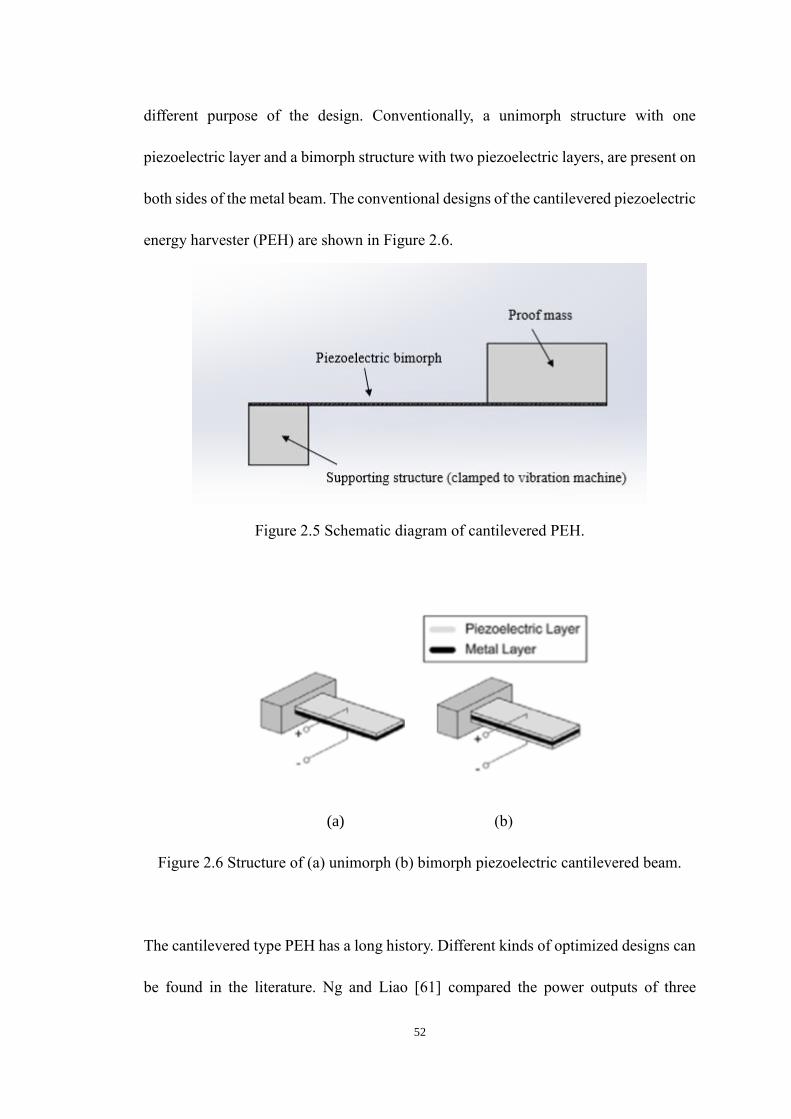
52
different purpose of the design. Conventionally, a unimorph structure with one
piezoelectric layer and a bimorph structure with two piezoelectric layers, are present on
both sides of the metal beam. The conventional designs of the cantilevered piezoelectric
energy harvester (PEH) are shown in Figure 2.6.
Figure 2.5 Schematic diagram of cantilevered PEH.
(a) (b)
Figure 2.6 Structure of (a) unimorph (b) bimorph piezoelectric cantilevered beam.
The cantilevered type PEH has a long history. Different kinds of optimized designs can
be found in the literature. Ng and Liao [61] compared the power outputs of three

53
cantilevered beam type piezoelectric energy harvesters which have different ways of
connecting the electrodes. They are a unimorph structure harvester with a parallel
connection, a bimorph structure harvester with a parallel connection and a bimorph
structure harvester with a series of connections. The results show that the bimorph
structure harvester with a series of connections has the largest range of load resistance
and operating frequency in which to generate peak power.
To improve the power output of a cantilevered type piezoelectric energy harvester,
Liang et al. [62] optimized the power output of the unimorph cantilevered beam
piezoelectric energy harvester with a fixed resonance frequency. In this study, the PEH
system was modeled using the energy method containing four geometric parameters
(length, width, thickness of the beam and the tip mass). The experiment results verified
that the optimal PEH was able to generate an output voltage of 3.95V. Sun et al. [63]
improved the performance of the typical cantilever PEH with an increase in
piezoelectric coefficient and electromechanical coupling coefficient material. The
optimized geometries of the device had been found with the maximum power output of
18mW. Cho et al. [64] improved the power output of PEH by improving the
electromechanical coupling coefficient in terms of applied stress, electrode coverage
and thickness of the beam and the piezoelectric layers. The electromechanical coupling
had been significantly improved by 150%. Du et al. [65] found the optimal electrode
cover area of the piezoelectric material for cantilevered PVEH and verified this with an
experiment. The results showed that the maximum power output of the cantilevered
PEH, which was 222nW, can be generated with 50% of the electrode area in the study.

54
Furthermore, there are many researchers focusing on the variant of PEH to improve the
power output, the traditional cantilevered type PEH has a narrow range of suitable
harvesting frequency (resonance frequency). The purpose of variants for a cantilevered
PEH is to produce a wider range of natural frequencies. Abdelkefi et al. [66] developed
a unimorph cantilevered PEH with a bending-torsion vibration tip mass as shown in
Figure 2.7. Similar to the unimorph cantilevered PEH, this device has an excitation base
connected with one end of the cantilevered beam, however, a two-end mass is connected
with the other end of the beam. The piezoelectric layer placed on the cantilevered beam
is thus subjected to bending and torsion force at the same time. Vibration with multiple
natural frequencies is achieved by different vibration mode shapes. The bending-torsion
vibration design and the optimal asymmetric tip mass design have improved the power
output by 30% compared to the symmetric tip mass design.
Figure 2.7 Schematic of the bending–torsion unimorph cantilever beam [66]
Xiong and Oyadiji [67] developed a double clamped multilayer structure PVEH. The
multilayer structures are shown in Figure 2.8, beams are connected with extra masses
(named M+1 and M-1) up to three layers. One of the beams is double clamped as an

55
excited base and two piezoelectric layers are located on both sides of the base layer. A
maximum of five vibration modes can be achieved by adjusting the position of the mass
and thickness of the base layer. The study shows that the optimal multilayer
cantilevered PEH can be used in different scales of vibration frequencies.
(a)
(b)
Figure 2.8 Double clamped multilayer structure PVEH: (a) double layers (b) triple
layers [67]
2.3.2.2 Cymbal type
Another significant PEH structure is the Cymbal transducer, its schematic diagram is
shown in Figure 2.9 (a). A typical cymbal transducer is designed as a circular shape,

56
configured with two metal endcaps on the top and bottom and the piezoelectric material
plate. Two electrodes are placed on the top and bottom of the piezoelectric plate. The
function of the endcap is to convert the vertical force from the top into a horizontal
force so that the piezoelectric material can operate in d33 mode which can generate a
higher amount of electrical power. The working mechanism of the Cymbal type
piezoelectric energy harvester is shown in Figure 2.9 (b).
(a)
(b)
Figure 2.9 (a) Schematic diagram of cymbal transducer (b) Force analysis of the
cymbal transducer [10].
The force amplification principle of the endcap can be expressed as the horizontal and

57
vertical result forces:
𝐹𝑦 = 𝐹
2 (2.28)
𝐹𝑥 =𝐹
2
1
𝑡𝑎𝑛𝜃≅
𝐹
2𝜃 when θ is small (2.29)
Thus, the force amplification factor of the endcap 𝐴𝑐 can be expressed as:
𝐴𝑐 = 𝐹𝑥
𝐹≅
1
2𝜃 (2.30)
The piezoelectric strain constant that related to the force amplification had been
proposed in the literature [54], which is called the equivalent strain constant 𝑑33𝑒𝑓𝑓
and
it is expressed as:
𝑑33𝑒𝑓𝑓
= 𝑑33 + |𝐴𝑑31| (2.31)
where 𝐴 = 𝑐𝑎𝑣𝑖𝑡𝑦 𝑟𝑎𝑑𝑖𝑢𝑠
𝑐𝑎𝑣𝑖𝑡𝑦 𝑑𝑒𝑝𝑡ℎ (2.32)
is dependent on the angle of endcaps’ leverage contributions, this equation shows how
piezoelectric constant 𝑑31 contributes to the piezoelectric constant through the angle
of endcap.
In order to improve the power output of the cymbal type PEH, Palosaari et al. [68]
optimized the Cymbal type PEH by finding the vibration frequency, applied force and
thickness of the steel endcaps. For a fixed diameter of 35mm and thickness of 540μm,
the optimal electrical power of 0.27mW was reported when the thickness of the steel
endcaps was 250μm and 24.8N force with the vibration frequency of 1.19Hz applied.
Kim et al. [69] studied the performance of the cymbal transducer with the fixed

58
diameter of 29mm and 1.8mm thickness. Results from FEA simulations and
experiments reported that the maximum electrical power of 52mW across the resistant
load of 400kΩ had been generated with the mechanical force of 70N at 100Hz. Yuan et
al. [70] improved the cymbal transducer by employing the analytical model, the
maximum electrical power output of the cymbal transducer under the force of 8.15N
was found around 1.56mW, with the resistant load of 390kΩ at the vibration frequency
of 120Hz. Ren et al. [74] modified the cymbal transducer into a rectangular shape to
make full use of the transverse extensional vibration of the PMN-PT crystal, for which
the piezoelectric effect of PMN-PT is anisotropic, the piezoelectric strain constant and
electromechanical coupling coefficient is ultrahigh. The study shows that a power
output of 14mW can be achieved under a cyclic force of 0.55N at the resonance
frequency of 500Hz, connected with a proof mass of 17g and load resistance of 74kΩ.
Tufekcioglu and Dogan [71] designed a PEH that combined two cymbal transducers
with a cantilevered structure, as shown in Figure 2.10. In this PEH, when the device is
subjected to vibration, two cymbal transducers convert the vertical force of the
cantilevered beam into the horizontal force and transfer the force to the PZT layer in
the middle of the cymbal device. This design enhances the fatigue life of piezoelectric
ceramic bodies by compressing the piezoelectric materials constantly. Design
parameters have been optimized by the analytical method and the finite element method,
and this has been validated by experiments. The aim of selecting design parameters is
to control the resonance frequency under the constraint of 200Hz whilst maximizing
the power output. For the cymbal structure of double piezoelectric layers, this PEH was

59
able to generate 141.61μW at 153 Hz, while a single piezoelectric layer cymbal
generates 104.04μW at 166 Hz.
Figure 2.10 3D sketch of PEH with two cymbal transducers [71]
Yuan et al. [72] studied the energy harvesting of a slotted-cymbal design [73], as shown
in Figure 2.11, which consists of a piezoelectric plate and two slotted metal endcaps.
Two silver electrode layers are located on the top and bottom surface of the piezoelectric
plate. The purpose of this design is to release the tangential stress which may cause
flexural motion to the piezoelectric plate and the loss of input energy. The study shows
that the 18-cone radial slotted cymbal is able to generate the highest electrical power of
16mW across the resistant load of 500kΩ. Compared to the original cymbal design with
the same thickness and diameters of the piezoelectric plate and the endcaps, the slotted-
cymbal had improved the power output by 60%.

60
Figure 2.11 Sectional schematic diagram of the slotted cymbal design [73]
Yuan et al. [70] introduced another slotted-cymbal transducer, which had been designed
with the circumferential slot between the horizontal and conical surface on the endcap.
The structure is illustrated in Figure 2.12. The purpose of the slot was to avoid the high
circumferential stress on the endcap which may reduce the efficiency of the mechanical-
to-electrical conversion. Experimental results showed that the energy conversion
coefficient increase was proportional to the depth of the slot. A maximum output of
2.5mW was found in the study, with slot depth of 0.35mm at the frequency of 120Hz.
This design improves the power output by 80% compared to the original cymbal
transducer.
Figure 2.12 Design of the circumferential slotted-cymbal transducer [70]

61
Traditional cymbal design and the designs introduced from the literature above have
the input limitation of less than 100N mechanical force. In order to scavenge bio-kinetic
energy from human walking, researchers have improved the endurance of the cymbal
device. Mo et al. [75] proposed a unimorph piezoelectric cymbal design of cymbal
transducer which can stand up to 1940N. Shown in Figure 2.13, the design replaces the
single PZT layer with a PZT/steel composite between the endcaps. Experiment results
show that the design with a substrate layer can generate a power of 121.2μW across the
load resistance of 3.3MΩ under 1940N at the low frequency of 1Hz.
Figure 2.13 (a) Traditional cymbal design (b) new design for the higher mechanical
load [75]
Another novel cymbal transducer for harvesting bio-kinetic energy from human footfall,
the Piezoelectric Flex Transducer (PFT), was developed by Daniels et al. [76]. In this
research, the PFT device was studied and geometric parameters were optimized by
using surrogate modeling techniques to maximize the power output. Details of the
development of the PFT device will be given in the following section.

62
2.4 The PFT device
2.4.1 Construction
The PFT device (as shown in Figure 2.14), was designed as a rectangular shape
containing two metal endcaps, one piezoelectric middle layer and two substrate layers
between the piezoelectric layer and two endcaps. Two electrode layers are located in
the top and the bottom surface of the piezoelectric plate, the resistor is connected
between them.
Figure 2.14 Structure of the developed PFT [76]
In developing the PFT, Daniels [76] created a coupled piezoelectric circuit finite
element model (CPC-FEM) for the Cymbal transducer, which was validated through
experiments. Based on the developed FEM, effects of geometric parameters and
material properties had been studied in order to find the optimal design and material for
the Cymbal transducer. In the study, eight geometric parameters (as shown in Figure
2.15) were selected as design variables. They are total diameter (D), cavity diameter
(Dc), apex diameter (Da), height (H), caps thickness (tc), PZT thickness (tp), join length
(J) and angle of the endcap (θ).

63
Figure 2.15 Schematic diagram of cymbal transducer with geometric parameters [76]
By varying one parameter each time, the maximum power of 0.12mW across the load
resistance of 10MΩ under 50N at 2Hz was found with the diameter of 30mm, 4.6 mm
in thickness of PZT and 0.33mm in thickness of endcaps.
The PFT had been developed based on the studies of the cymbal transducer. The
purpose of the design is to enable the cymbal transducer to harvest bio-kinetic energy
from human walking. Two substrate layers between the endcaps and the piezoelectric
plate were designed to avoid all the force from the endcap transfer across the surfaces
of the piezoelectric material causing the mechanical failure of delamination. Thus, the
role of two substrate layers was to enable the PFT to operate under a high load which
is up to 1kN and low-frequency environments by increasing the vulnerable interface
between the endcaps and the piezoelectric plate. The rectangular shape of the PFT
device was designed to increase the packing factor and the use of the space whilst
integrating it into a shoe for harvesting energy from human walking.
The effect of geometric parameters and material properties had been studied by Daniels
[76] using FEA. The original design parameters of the PFT are based on the previous

64
study of the cymbal transducer. To study the effect of design parameters on the power
output, eight geometric parameters were selected. The values of the original geometric
parameters are listed in Table 2.2, they are total length (D), cavity length (Dc), width
(w), apex length (Da), heights of endcaps (H), caps thickness (tc), piezo thickness(tp),
join length (J) and angle of the endcap (θ). Amongst the design parameters, the
thickness of the piezoelectric layer, the angle of the endcap and the joint length are
picked from the optimal design of the cymbal transducer.
Table 2.2 Geometric parameters of PFT before optimization
Total Length (mm) D 52
Cavity Length (mm) Dc 40
Width (mm) w 30
Apex Length (mm) Da 14
Height (mm) H 3.5
Endcap Thickness (mm) tc 2
Piezo Thickness (mm) tp 4
Join Length (mm) J 6
Angle of the Endcap (°) θ 8.75
Similar to the geometric parameters, material properties were optimized by Daniels [10]
by using CPC-FEM to investigate its effects on the power output. Six material
properties of the piezoelectric material were selected as design parameters including
the elastic compliance (s11), piezoelectric strain constant (d31), piezoelectric voltage
constant (g31), the relative dielectric constant (εr33T
), piezoelectric coupling coefficient
(k31) and FOM (d312/εr33
T ). After optimization using the one parameter a time approach,
piezoelectric material DeL Piezo DL-53HD was selected. Materials used for the

65
developed PFT and its properties are listed in Table 2.3. The piezoelectric coefficients
have been described in the previous section. The damping ratio of the piezoelectric
material is determined by the mechanical quality factor Q. This is a dimensionless
parameter that describe the resonance behavior of an underdamped harmonic oscillator
or resonator. The relationship between damping ratio and Q factor can be expressed as:
ζ = 1
2𝑄 (2.33)

66
Table 2.3 Material properties used in the study of PFT
2.4.2 The developed CPC-FE model of PFT
To study the performance of the novel PFT device, Daniels [10] developed a CPC-FEM
to analyze the effect of geometric parameters on the power output. This model was
created by employing the multi-physics FEA software ANSYS (version 13) [13]. The
FE model with its components and the mesh is shown in Figure 2.16. In this model, the
element type SOLID226 was selected for the PZT plate. This element is a 3-D couple
AK Stainless Steel: Austenitic stainless steel 304, MatWeb, LLC
Young's Modulus (GPa) 193
Yield Strength (MPa) 251
Density (Kg/m3) 8030
Poisson's Ratio 0.24
Piezoelectric Material: DeL Piezo DL-53HD
Elastic Compliance (x10-12 m3/N)
S11 15.1
S12 -4.5
S13 -9.4
S33 24.8
S44 37.1
S66 39.2
Relative Dielectric Constant (at constant stress)
εr11T
3550
εr33T
3850
Density (Kg/m3) 7900
Piezoelectric Strain Constants (x10-12 m/volt)
d15 810
d31 -300
d33 680
Piezoelectric Coupling Coefficient k31 0.42
Mechanical Quality Factor Q 20

67
field hexahedron of 20 nodes and suitable for the analysis of piezoelectric structural
responses. SOLID95 was selected for endcaps, which is also a hexahedral element type
with 20 nodes. CIRCU94 was used for the resistor connected between the positive and
negative electrodes. The fix base is set in the bottom of the device, electrode layers are
in the top and the bottom surface of the piezoelectric layer between the substrate layers
and the load resistance is connected between electrodes. In order to obtain the power
output of the device, the FEM was subjected to 1kN distributed load with 2Hz on the
top apex of the device.
Figure 2.16 The FEM of PFT with components and mesh
After optimizing by changing one parameter at a time, as in the previous study of the
traditional cymbal device, optimized geometric parameters were selected (listed in
Table 2.4).

68
Table 2.4 Optimized design parameters of PFT
Total Length (mm) D 52
Cavity Length (mm) Dc 40
Width (mm) w 30
Apex Length (mm) Da 14
Endcap Thickness (mm) tc 2
Piezo Thickness (mm) tp 4
Substrate layer thickness (mm) ts 0.6
Angle of the Endcap (°) θ 8.7
Lastly, the PFT device was fabricated and tested based on the optimal design parameters.
To test the prototype of the PFT, the PFT device was connected to a range of load
resistance from 0 to 10 MΩ and the mechanical input was given by a 1.5kN payload of
the loading machine. The experiment set up used to test the PFT is shown in Figure
2.17 and the equivalent electrical circuit of the PFT including the resistance (R),
capacitance (C1, C2) and inductance (L1) is shown as Figure 2.18. The data was taken
from different input loadings and vibration frequencies.
Figure 2.17 Experiment set up for PFT testing [10].

69
Figure 2.18. The equivalent circuit of the PFT device [10].
One comparison of the experiment and simulation results is shown in Figure 2.19. This
figure plots the results that the PFT was testing with 5Hz excitation frequency.
Figure 2.19 Comparison between experiment and simulation results of PFT device
under input load at 5Hz. [10]
Combining Figure 1.6 and Figure 2.19, both comparison studies above have shown
that a non-negligible error has occurred between the simulation results and the
experiment results. As mentioned in the previous chapter
In this research the accuracy of the FE model will be studied and further developed
with improved accuracy.

70
2.5 Optimization techniques
In the literature there are different optimization techniques for optimizing engineering
designs, for example the one factor a time using the FE method and the analytical
model method. As the design becomes more complex in recent times, surrogate
models are often employed for optimization. In this research, the electric output of the
novel PFT energy harvester will be improved efficiently and effectively by employing
the surrogate model assisted optimization method. This methodology optimizes the
PFT device by following steps: (i) the experiment of the PFT is approximated by FE
model in order to study the behavior of the device at a lower cost; (ii) with the design
of the computer experiment, the design space is sampled within the selected design
constraints and the sampled data are simulated by FEA; (iii) using the results of FEA,
the relation between output parameters and the input design variables can be
approximated within the design space by surrogate models; (iv) the surrogate models
can be optimized by numerical optimization algorithm and (v) the result will be
validated by FEA. The following subsections will give an overview of optimization
techniques which were employed in the surrogate model assisted optimization
method, they are Finite Element (FE) method, Design of Experiments (DoE),
surrogate modeling techniques and numerical optimization techniques.
2.5.1 Finite Element (FE) method
Traditional engineering optimization processes require a large number of expensive
experimental tests from prototypes which may be unaffordable and ineffective.

71
Benefiting from the rapid development of computer-aided design engineering, finite
element analysis, which can numerically predict the performance of a design by virtual
computer experiments, has become the most popular method to replace the traditional
design process so that the cost of the experimental tests can be greatly reduced.
The finite element method is one of the popular computer-aided modeling methods to
approximate the differential equation of complex engineering problems. This modeling
method has the advantage of convenience and that it can be used in different fields. In
this research, the prototype of the PFT device will be approximated using the Finite
Element Model (FEM). According to the literature, the governing equation of
piezoelectric energy harvesting via FEM can be expressed as:
{D} = [e]T{S} + [α]{E} (2.34)
{T} = [β]{S} - [e]{E} (2.35)
In these governing equations, {D} is the dielectric displacement vector and {T} the
stress vector, [e] is the dielectric permittivity matrix, {S} is the strain vector, [α] is the
dielectric matrix at constant mechanical strain, {E} is the electrical field vector, and [β]
is the matrix of elastic coefficient at constant electric field strength.
Alternatively, the established equation for strain and electrical displacement, given by
IEEE [85], is as follows:
{S} = [sE]{T} + [d]{E} (2.36)

72
{D}= [d]T{T} + [εS ]{E} (2.37)
Different from the equation used by FEM, in these constituted equations {S} is the
strain vector, [sE] is the compliance matrix at the electric field, [d] is the piezoelectric
matrix relating strain and electric field and [εS] is the dielectric matrix evaluated at
constant strain. Matric form of the constituted equations and the input method of the
piezoelectric material properties to the ANSYS FEM software based on the equations
have been introduced in Daniels [76]. In this research, the FE model will be constructed
and analyzed by the FEA software ANSYS APDL and the input method used by
Daniels [76] is employed.
In the literature there are many successful engineering designs that have used FEM.
The first FEM textbook was published by Zienkiewicz and Cheung [77] in 1967. Since
then, FEM has been used widely on a number of engineering design problems. The
fundamentals of FEM were given by Barkanov [78], along with an example of
modeling a shaft system using FEM and other modeling methods for comparison. Sohn
et al. [79] developed FE models for piezoelectric thin films to evaluate the electric
output of the piezoelectric material under stress. The results were validated by an
analytical model and experiments which concurred. Marco et al. [80] developed the
FEM of acoustic levitator and used the model to determine the optimal geometries of
the device. The optimal design of the acoustic levitator was produced and then verified
by the experiment, the results had closely matched those from FEA. Amira et al. [81]
performed FEA on a thin-filmed, multi-layer piezoelectric pressure sensor to obtain the

73
maximum deflection and the voltage generation of the piezoelectric layer. In this case
the optimal material properties for the application had been selected. Leinonen [82]
developed an FEM for a piezoelectric cymbal harvester to calculate the power
generation. The results showed that when compared with the prototype the developed
FEM had a minor error of 7% compared to the experiment and that the optimal
resistance load of the device had been predicted successfully. Tabatabaei et al. [83]
optimized the shape of the beam for the piezoelectric cantilevered energy harvester
using the analytical model and verified the optimal design with the results obtained
from the FEM simulations. Zhu et al. [84] developed a coupled piezoelectric-circuit
finite element model (CPC-FEM) for the cantilevered piezoelectric energy harvester.
This model connects the cantilevered beam with the piezoelectric layer and a load
resistor to predict the electrical power output directly from the FEM including load
resistance. The study found that the electric output of cantilevered PEH is highly
dependant on the load resistor and the relationship is nonlinear.
2.5.2 Design of Experiment (DoE)
The design of experiment is the first step towards creating a surrogate model which is
used to generate the input data in a given design space. The selection of DoE will affect
the efficiency of surrogate modeling and the convergence of the model. The most basic
DoE techniques are factorial designs. In factorial designs, the variables used to predict
the approximation model are called factors. The most basic types of factorial design
include full factorial design [86, 87], fractional factorial design [88, 89] and central

74
composite design [90,91]. Full factorial design of experiments generates all design
variables to create the surrogate model. For example, full factorial DoE generates 2k
design variables to approximate the model when the experiment has k factors with 2
levels in each factor. In DoE, factors are used to represent the design variables and
levels are the possible values of the design variables. Figure 2.20 (a) demonstrates a 23
full factorial design, the black dots represent the experiment designs. This methodology
has the advantage of high accuracy in approximation, however, the number of designs
will increase exponentially with the number of design variables and levels to be
estimated, thus it is also time-consuming and expensive. Fractional factorial DoE is
often used when the number of factors is large. This DoE technique reduces the
estimation of main factors, and the reduced main effect of the factors are aliased by the
interactions between factors. Figure 2.20 (b) demonstrates the fractional factorial
design with 23-1 runs. Fractional factorial designs are normally indicated as 2𝑅𝑘−𝑝
,
where R is the resolution of the experiment or the number of main effects to be aliased,
for Figure 2.20 (b), aliasing effects are x1, x2, x3, the fractional factorial design can be
denoted as 2III3−1.
The Central Composite Designs sampling technique is commonly used to fit the second
order models. This technique generates 2k full factorial design or 2k-p fractional factorial
design points, plus 2k axial points and one centre point to explore the quadratic effects
of the model. Figure 2.20 (c) demonstrates the Central Composite Design, sampling
points are indicated by the black dots.

75
(a) (b) (c)
Figure 2.20 Three types of factorial design: (a) 2III3 Full Factorial (b) 2III
3−1
Fractional Factorial (c) Central Composite Design
Besides the factorial designs, a number of optimal designs have been proposed based
on different optimality criteria. For example, the D-optimal computer-aided design base
on the d-optimality criteria reduce the number of designs from the full factorial design
depending on the determinant of the combination matrix. The larger determinant of the
selected combination matrix X'X indicates that the sampled design has spanned a wider
volume of the design space. Details of the optimal design of experiments with different
optimal criteria have been reviewed by Triefenbach [92].
An efficient and economic DoE technique suitable for fitting second order polynomial
surrogate models named Box-Behnken designs is derived by Box and Behnken [93].
This technique employs incomplete 2k factorial design blocks in sampling designs. For
the most part these designs are rotatable and can be orthogonally blocked, which are
two desirable properties of the second-order response surface model.
Plackett–Burman designs is a DoE technique suitable for 2-level design. In this method,
the interaction between factors is ignored and only the main effects are considered in
order to reduce the number of designs from the complete factorial design. Details of the

76
method can be found in Plackett and Burman [94]
The Taguchi method [95] employed the orthogonal array of DoE technique to
investigate the effect of factors in reducing the sensitivity of the design. In the
orthogonal array, factors are divided into control factors and noise factors. Control
factors are parameters where value can be controlled. These factors are listed in the
inner array while noise factors (uncertainties) are set in the outer array. Experiments are
conducted with inner and outer arrays to estimate how the noise factors affect the
control factors, and how these eventually lead to the reduction in sensitivity of the
design.
Latin hypercube DoE developed by Mckay et al. [96] is a sampling technique that
generates designs from the design space uniformly. The number of samples to be
generated could be any population decided by the designer before sampling. The design
space will be divided into uniform subsets depending on the number of samples that
being decided, then one design is generated in each subset in order to generate uniform
samples.
2.5.3 Surrogate modeling
Due to the increase of design complexities, the combinations of different design
parameters increase exponentially with either the number of design variables or the
level of each variable. For instance, a system design with 7 variables and 2 levels of
each will have 27 which is 128 possible designs, 7 variables with 3 levels of each will
cause 37 which is 2187 designs, etc. To explore all of these possible designs using FEM

77
with a fine mesh becomes expensive and impractical. At this point, surrogate models
are often employed to approximate the original FE simulations so that the design
optimization can be predicted efficiently by using the mathematical algorithm. In this
subsection, some basic and popular types of surrogate modeling techniques will be
introduced.
2.5.3.1 Interpolation
Surrogate modeling techniques can be divided into two main types, mathematical
modeling, and artificial intelligence modeling. One of the most basic mathematical
surrogate modeling methods is interpolation. There are different types of interpolation,
depending on the model that is selected, for example, linear, polynomial or spline
interpolation. In this method, the real model is approximated by the response of
interpolating points and the selected function. The simplest method of interpolation is
the linear interpolation. This method connects two nearest sampling points with a
straight line, the function used for approximation in linear interpolation can be
expressed as:
𝑦 − 𝑦1
𝑥 − 𝑥1=
𝑦2 − 𝑦1
𝑥2 − 𝑥1 (2.38)
where (x1, y1) and (x2, y2) are interpolation points.
Clearly, it is suitable for approximating first-order linear functions but the error will
become unavoidable while approximating curve functions since only finite

78
interpolating points can be created.
For a complex design problem, the method often used to interpolate function is
polynomial interpolation rather than linear interpolation. This method is used to
interpolate the sampling data, approximate the real function by polynomials and
construct a polynomial with the degree of the most n, where n is the number of
interpolation points. For example, the interpolation polynomial created by Lagrange
has formed the equation:
Ln(x) = 𝑓(x0)λ0(x) + 𝑓(x1)λ1(x) + … + 𝑓(xn)λn(x) = ∑ 𝑓(𝑥𝑘)𝑛𝑘 𝜆𝑛(𝑥) (2.39)
where λk = (𝑥− 𝑥0)(𝑥−𝑥1)…(𝑥−𝑥𝑘−1)(𝑥− 𝑥𝑘+1)…(𝑥− 𝑥𝑛)
(𝑥𝑘− 𝑥0)(𝑥𝑘− 𝑥1)…(𝑥𝑘− 𝑥𝑘−1)(𝑥𝑘− 𝑥𝑘+1)…(𝑥𝑘− 𝑥𝑛)
Polynomial interpolation has the ability to approximate the real function with higher
accuracy, however, for a large number of interpolation points, the polynomial
interpolation will become time-consuming to create a high dimension polynomial.
Details of the interpolating method and other mathematical approximating functions,
such as the construction of polynomial interpolations and the Taylor Series
approximation, can be found in Kincaid and Chene [97].
2.5.3.2 Polynomial fitting and Response Surface Method (RSM)
One of the most popular mathematical modeling techniques recently is polynomial
fitting. The difference between polynomial fitting and interpolation is that polynomial

79
fitting involves finding a solution that closes to the data points with smoothed function
while interpolation is to create the function through the relationship between the
interpolating points.
A general form of polynomial can be written as:
yi = β0 + β1xi + β2𝑥𝑖2 + … + βmxm + εi (i = 1,2,…,n) (2.40)
where yi is the response of the function, x is the independent variable, β is the linear
coefficient to be evaluated and εi is the zero-mean random error. The significance of
different independent variables can be identified by the coefficient β from the
normalized polynomial model, thus the design problem can be simplified by reducing
the ineffective design variables. Furthermore, noise functions can be reduced, and the
model can be converged efficiently with its smooth property. However, the coefficient
will be difficult to evaluate, and the model becomes highly inaccurate as the complexity
of the design problems increase. The polynomial regression is thus suitable for
approximating linear or second-order design problems.
Similar to polynomial fitting, the Response Surface Methodology (RSM), as proposed
by Box and Wilson [98], is used to approximate the model with a higher dimension. In
this method, the second-order polynomial regression model is often suggested since its
derivative can be easily calculated for ease of finding the optimal value of the problem.
Errors between the function and the data are assumed to be normally distributed with
mean zero and standard deviation σ. The regression coefficients are determined by the

80
factorial design of experiments and the least squares regression analysis to fit the data.
Examples of solving mathematical problems using response surface methodology are
given in Box and Wilson [98].
2.5.3.3 Artificial Neural Network (ANN)
In artificial intelligence surrogate modeling techniques, one of the basic modeling
methods is the Artificial Neural Network. This method creates the surrogate model
through components called neurons. Typically, the neural network surrogate model
includes multiple linear regression models with a nonlinear transformation [99]. A
simple neural network including a single input neuron is demonstrated in Figure 2.21.
It includes input p, weight w, bias b, net input n, transfer function f and output a.
Figure 2.21 Schema of single input neural network [99]
Most commonly, the weight function w is used to multiply the input p and the net input
is constructed by summing weighted inputs with the bias, thus, the simple network
shown in Figure 2.21 is expressed as:

81
f(𝑛) = f(𝑝 ∗ 𝑤 + 𝑏) (2.41)
Another important component of ANN is the selection of transfer function. The most
commonly used transfer function to create the surrogate model is the sigmoid transfer
function since its derivative of this function can be easily calculated. For example, the
neural network created by sigmoid transfer function can be expressed as:
y = 1
1 + 𝑒−𝜂/𝑇 (2.42)
where η = ∑𝑤𝑖𝑥𝑖 + 𝛽 , 𝛽 is the bias of the input and T is the coefficient of the
selected sigmoid transfer function.
Creating surrogate models with the neural network can be concluded in 5 main steps:
• data collection
• network creation
• initializing weight and bias
• network training
• network validation.
To create a surrogate model by using a neural network, a back propagation algorithm
is commonly used. In this algorithm, first, an initial network is defined with the
weight and bias. The output data is compared with the target value of the real model,
error between the output and the target value will be used to propagate the input and
adjust the weight and bias. The training process will be repeated until the error

82
satisfies the defined value. The ANN was recorded that the outputs are a regression-
type function, it is suitable for approximating the regression applications, however,
the data training may be computationally expensive if the data is of a large volume.
2.5.3.4 Kriging
The kriging surrogate modeling method was introduced by Sack [100] and recently it
is often employed in the literature. The kriging modeling method creates a model with
polynomial regression plus the error between the predicted function and the regression
model. The general form of a kriging model can be expressed as the equation:
Y(x) = ∑𝛽𝑗𝑓𝑗(𝑥) + 𝑍(𝑥)
𝑘
𝑗=1
(2.43)
where ∑ 𝛽𝑗𝑓𝑗(𝑥)𝑘𝑗=1 is the traditional response model and Z(x) is the stochastic process
with zero-mean, variance 𝜎2, and covariance [101]
𝐶𝑜𝑣[ 𝑧(𝑥𝑖), 𝑧(𝑥𝑗)] = 𝜎𝑧2𝑅(𝑥𝑖, 𝑥𝑗) (2.44)
where R (xi, xj) is the correlation function. Most commonly used correlation functions
are an exponential function, Gauss function and Cubic-spline function. Expressions of
correlation function can be found in Ryu et al. [102]. For a complex design problem,
the kriging model has been shown to have a small oscillation and a better fitting
compared to polynomial fitting. Many researchers employ kriging surrogate modeling

83
for a fast optimization in the literature, examples can be found in [103-107].
2.5.3.5 Genetic Programming (GP)
Genetic programming methodology (GP) is an optimization technique that belongs to
the Evolution Algorithm (EA) [106]. GP is not only capable of finding the optimal
solution of the problem but also the better coefficient or operators of the surrogate
model. The genetic programming code was first developed according to the guidelines
provided by Koza [107], then implemented for symbolic regression tasks by Armani et
al. [108]. This modeling method is based on Darwin’s evolution theory in which the
species that fit the environment survive by the process of natural selection. Similar to
the reproduction process of species, this modeling methodology starts with an initial
user defined individual (surrogate model) including model data and operators. The
computer program generates a number of populations iteratively by operations such as
mutation and crossover etc., each generated individual will be examined by a fitness
function, the one with better fitness to the given data will survive and finally the
programming process stops if the output reaches the design criteria, such as number of
populations or the model fitness. A typical tree structure used to represent an individual
function in GP is shown in Figure 2.22. This individual representing a mathematical
expression of (𝑥1
𝑥2+ 𝑥3)
2
, the subtree structures will be varied during the modeling
procedure and the one with better fitness rank will survive and pass to the new
generation.

84
SQ
+
/
Binary Nodes
Unary Node
Terminal Nodes
x 1 x 2
x 3
Figure 2.22. Typical tree structure for (𝑥1
𝑥2+ 𝑥3)
2
.
The process of the GP methodology can be concluded and schematically shown in
Figure 2.23. More details and implementations about genetic programming can be
found in Armani [109].

85
Figure 2.23. A flowchart of Genetic Programming methodology.
Since the GP surrogate modeling technique has the advantage of easy handling, and the
surrogate model is inexpensive to evaluate, the GP method will be employed in this
research for surrogate modeling in order to approximate the relation between the output
of the FEM and design variables of the PFT energy harvester.
INPUT
Structure initialization
Parameters tuning
Fitness evaluation
Parameters insertion
Parameters removal
Structure sorting
Structure selection
Genetic operations on structure
New population
Acceptable
quality? Result

86
There are many successful engineering designs that employ surrogate modeling in the
literature. Examples include: Kim et al. [110] employed the kriging surrogate modeling
method to maximize the electrical power output of the piezoelectric cantilevered energy
harvester. The kriging surrogate model was constructed by optimal Latin Hypercube
(OLH) sampling to approximate the relation between selected geometric parameters
and the electrical power, natural frequency and mass. The model predicted the optimal
design successfully which has 208.02% improvement compared to the original design.
Cappelleri et al. [111] optimize the tip force and deflection of a thickness varying PZT
bimorph actuator for minimally invasive surgery. The study approximates the global
design space by using both response surface model and a kriging model, the kriging
surrogate model shows the advantage of approximating the nonlinear problem in the
study. With a Pareto frontier result given by the kriging model, the optimal design
variables are selected for a sufficient performance of the device. Marcelin [112]
introduced a numerical optimization approach that approximates the design problem by
the neural network and the optimal solution is calculated using GA. The methodology
is then demonstrated to optimize a car gearbox mechanism with 2 beams and 3 bearings
for minimizing the deflection of the beams. Araújo et al. [113] estimate the elastic and
material properties of the active plate structure with surface bonded piezoelectric
patches by employing both artificial neural network (ANN) and numerical gradient-
based optimization methods. The aim of the study is to find the design parameters while
the system operates at eigen-frequencies and to minimize the error between the FE
model and experiment results. Both methods showed a good performance in the study

87
to estimate the parameters but the ANN is computationally more costly.
2.5.4 Numerical optimization techniques
After the engineering design problem has been approximated by surrogate models, the
optimal design can be found by solving the problem with numerical optimization
techniques. There are many approaches that can be used to solve the mathematical
optimization problem. These approaches can be categorized into two types: the
optimality criteria methods and the search method. The optimality criteria method finds
the optimal solution based on the optimality criteria, while the search method finds the
optimal result iteratively from a given starting point in the function.
Most of the optimization techniques have been described by Arora [114]. This section
will focus on the numerical optimization techniques that are commonly used to solve
non-linear constrained design problems. Two optimal searching methods and a nature-
inspired method are introduced in the following, they are Sequential Linear
Programming, Sequential Quadratic Programming, and Genetic Algorithm.
Generally, the search methods that are used to solve nonlinear problems is to linearize
the problem at a given design and consider the optimization problem at the current point
as a linear subproblem. SLP is the numerical method that treats the subproblem of a
given design point as a standard linear programming (LP) optimization subproblem.
The given point moves to a new location by calculating the gradient and move step of
the current point, then the LP process will be repeated.
The linearization of the cost function and constraints of the problem are implemented

88
by employing the linear Taylor’s expansions, thus the linearized cost function and
constraints of the problem at the design x with kth iteration are expressed as:
Minimize
𝑓(𝑥𝑘 + Δ𝑥𝑘) ≅ 𝑓(𝑥𝑘) + ∇𝑓T(𝑥𝑘)Δ𝑥𝑘 (2.45)
Subject to
ℎ𝑗(𝑥𝑘 + Δ𝑥𝑘) ≅ ℎ𝑗(𝑥
𝑘) + ∇ℎ𝑗T(𝑥𝑘)Δ𝑥𝑘 = 0; j = 1 to p (2.46)
𝑔𝑗(𝑥𝑘 + Δ𝑥𝑘) ≅ 𝑔𝑗(𝑥
𝑘) + ∇𝑔𝑗T(𝑥𝑘)Δ𝑥𝑘 ≤ 0; j = 1 to m (2.47)
where 𝑓(𝑥) is the cost function, ℎ𝑗(𝑥) and 𝑔𝑗(𝑥) represent the equality constraint
and inequality constraint, respectively. According to the Taylor’s expansions, ∇𝑓, ∇ℎ𝑗
and ∇𝑔𝑗 are the gradients of the cost function, the equality constraint and the
inequality constraint at the kth iteration, respectively. Δ𝑥 is the change of the design
variable 𝑥. After the problem has been linearized, the minimization of the cost function
becomes a problem of finding the Δ𝑥.
2.5.4.1 Sequential Linear Programming (SLP)
To find the optimal solution using SLP algorithm, the linearized subproblem is
simplified as a linearized change of the cost function, which expressed in matrix form
as follows:

89
Minimize
𝑓̅ = cT d (2.48)
Subject to
NTd = e (2.49)
ATd ≤ b (2.50)
where the matrices c, N, A are the gradient matrix of the cost function, equality
constraint and inequality constraint, respectively, d is the move step along the direction.
The linearized LP subproblem can be solved by a standard Simplex method [114] which
is commonly used to solve the LP problem. The procedure of the SLP algorithm can be
concluded as following,
1) Estimate a starting point with iteration k = 0 and set the permissible tolerance which
is a small allowable distance between the current point and the new point.
2) Calculate the value and gradient of the cost function and constraints at the starting
point and define the LP subproblem with equation (2.45)-(2.47).
3) Select a proper move limit for the searching procedure
4) Solve the LP subproblem by the standard Simplex method to find the move step d.
5) Check for convergence, stop if it satisfies the preset permissible tolerance,
otherwise, continue.
6) Update the starting design with the new design as a new iteration k+1, and go to
step (2).

90
The SLP technique is a simple and direct approach to solve the optimization problem,
however, this algorithm shows some disadvantages:
• The optimal solution search by SLP may not converge to the minimum precisely,
and the searching process may repeat between two points.
• A proper move limit is required to be selected before the search process is executed.
The move step can be found by a trial and error approach which may be time-
consuming.
2.5.4.2 Sequential Quadratic Programming (SQP)
To overcome the drawbacks of the SLP algorithm several derivative-based methods
have been developed to solve the nonlinear optimization problem. The SQP is one of
these derivative-based optimization techniques that is able to solve the problem with
both equality and inequality constraints accurately and effectively. The main process of
SQP is to approximate the cost function of the optimization problem using quadratic
functions and to solve the quadratic subproblem iteratively until the optimization
problem has been solved.
The first and basic step of SQP is to approximate the cost function using a quadratic
function and to formulate the linearized optimization problem into a QP subproblem.
The approximation of the QP subproblem is expressed as:
Minimize
𝑓̅ = cT d + 1
2dTd (2.48)

91
Subject to
NTd = e (2.49)
ATd ≤ b (2.50)
where matrices c, N, A are the gradient matrix of the cost function, equality constraint,
and inequality constraint, vector d is the search direction. The factor of 1
2 with the
second term in Eq. (2.48) is introduced to eliminate the factor of 2 during differentiation.
Since the QP subproblem is formulated as a convex, the minimum point of the
subproblem is unique and it can be found by solving the problem in different ways. The
search direction d can be computed by solving the subproblem and the step size of the
QP problem can be calculated as the minimization of the descent function. Thus, this
technique is more popular than the SLP technique, since it can converge to the local
optimal point faster. In this research, the SQP will be employed to find the optimal
design of the PFT energy harvester after the design problem is approximated by
surrogate models.
2.5.4.3 Genetic Algorithm (GA)
Owing to the complexity of the design problems, local optimization techniques are not
able to guarantee finding a global optimal design of the nonlinear design problem when
the problem has more than one local optimum. In this case, Global optimization
techniques will be employed.

92
GA is one of the natural-inspired global optimization methods that are general and easy
to handle. As per the previous description of the GP modeling technique, GA is also
one of the classifications of EA, which is inspired by Darwin’s theory of evolution by
natural selection. GA searches the optimal solution by the following steps, 1) start with
a given initial design, 2) generate a set of design candidates within the design space, 3)
evaluate the design randomly, 4) a subset of new designs is generated with a bias of
selecting design variables that lead to a better result, 5) this optimization process stops
if the design satisfies the preset criteria. The most important step in GA is the generation
of new populations, this process is implemented by operation of reproduction, crossover,
and mutation. Reproduction is the process that generates a new population from the
previous one, by selecting the members that cause a better fitness during the evaluation.
As a result, designs in the new population will show a better result compared to their
parents.
Crossover is the process that combines the characteristics between two different designs
within the new population in order to further improve the result of the fitness function.
The most popular methods of crossover are the one-cut-point and the two-cut-point
method. The operation of crossover with the one-cut method is illustrated in Figure 2.24.
x1 and x2 in Figure 2.24 (a) are two sets of design that are encoded into a binary string.
The cut point is decided as 4 digits from the right end and the designs exchange base
on this cut point. New designs are generated as Figure 2.24 (b) which is x1’ and x2’.

93
Figure 2.24 Crossover with one-cut point method. (a) Binary string before crossover
(b) after crossover [114]
Mutation is the operation that selects the member randomly from the new population
and changes the value of the member. As an example, the binary string x1 shown in
Figure 2.24 which has a value of 10 1110 1001. To execute the mutation process, one
of the numbers will be selected and switch from 0 to 1 or vice versa. If the location 4
from the left side is selected, x1 will become 10 1010 1001. The purpose of this
operation is to prevent the loss of a better gene during the reproduction and crossover
process.
By its random search process, GA is able to find the global optimal within the given
design space for all types of design problems, such as constrained and unconstrained
problems. Thus, this method is easy to execute and it is a general global optimization
technique. It is worth noting that to deal with the constrained problem using GA, the
problem will be reformulated to an unconstrained problem by the penalty function. This
optimization method will be employed in this research to find the global optimal
solution while proceeding the multi-level surrogate modeling.

94
2.6 Summary
In this chapter, the literature review of piezoelectric energy harvesting, including the
mechanism of cantilevered type and cymbal type PEH, the development of novel PFT
device and the recent optimization techniques have been discussed. The PFT has been
developed with a higher standing force and it can be embedded into a shoe to harvest
the bio-kinetic energy from human walking. However, the optimization of PFT in
previous research employed the traditional one parameter each time methodology
which changes one design parameter and keeps the remaining others constant. This
method ignores the effects between different design parameters during the optimization
process. In this research, the novel PFT device will be optimized by using the surrogate
model assisted optimization techniques. The design parameters will be generated
uniformly from the design space as input data and then analyzed by an FE model, and
both input and output data will be used to construct surrogate models which are able to
represent the behavior of the FEM. With the convenience of the surrogate model, the
optimal design of PFT will be found efficiently by using mathematical optimization
techniques. The result of optimization in this research will be compared with previous
studies to prove that recent advanced optimization techniques have the advantages of
efficiency and reliability. The optimized PFT energy harvester is expected to generate
a higher power compared to previous studies.
In the following chapter, the FEM of PFT will be further developed in order to improve
its accuracy so that the error between the result of FEM and the experiment can be
reduced.

95
Chapter 3
Further development of the FE model of the PFT
The aim of this chapter is to improve the accuracy of the existing finite element (FE)
model of PFT by changing the size of the element (mesh size). As mentioned in the
previous chapter, the results obtained by the FE model has a non-negligible error
compared to the experimental results. This error can be explained by two main reasons,
the first reason is the inaccuracy of the FE model itself with the large size of elements,
which means the developed FE model has a coarse mesh. FE models with a large size
of elements are capable of providing the results within a short computational time in
the simulations, however, the inaccuracy of the FE models cannot predict the result
accurately due to the lack of convergence. As a result, the cost of simulations to predict
the performance of the designs, as well as the experimental validations may be
prohibitive. The second reason for the error between the results of FE model and
experiments is the inappropriate equipment used in the experiment. According to
Daniels [10] who developed the FE model and validated it by experiments, the
experiment employed a 20kN load cell to monitor the loading of 1kN on the PFT instead
of using the 1.5kN load cell since the 1.5kN load cell was unavailable. The 20kN load
cell had an unsuitable working force range for the experiment and thus the error had
occurred. In this chapter, the first reason will be considered and the CPC-FEM will be
further developed by improving its accuracy.
FE models with a coarse mesh will cause the inaccuracy of the result, on the other hand,

96
decreasing the mesh size of the model leads to a relatively accurate model but a longer
simulation time. The trade-off between model accuracy and the computational time of
the FE model is needed to be considered before the use of the model. In this study, the
accuracy of the FE model will be addressed by referring to three electrical output
parameters including current, voltage and power, and the mechanical output parameter
which the von mises stress of the endcaps. An appropriate mesh size and computational
time will be selected based on the stability of the outputs. The improved FE model will
be employed for the further study to optimize the power output of the PFT device.
3.1 Convergence analysis of the developed PFT
The developed FE model should converge to the experiment so that the model can be
used to represent and predict the performance of the system. A good convergence of the
FE model means the solution of the FE model is close to the solution of the experiment.
Generally, increasing the accuracy of the FE model can be achieved by reducing the
size of the element, however, reducing the size of the element will be penalized by a
significant increase of computing time because the number of elements will be
increased rapidly. The original FE model developed by Daniels [10] is shown in Figure
3.1, this model includes 1101 elements and 6437 nodes. The size of its elements is 3
mm3. The lack of convergence of the developed FE model has been mentioned in the
previous chapter, results of this FE model have a large error compared to the
experimental results. This error could be reduced with an appropriate mesh size.
To analyze the convergence of the original FE model simulations will be executed with

97
the boundary conditions shown in Figure 3.1 and concluded as follows:
• The fixed base is set at the bottom endcap
• Distributed load is applied at the top endcap
• The top and bottom surface of the piezoelectric plate are set as two electrodes
• The load resistor is connected between two electrodes
Figure 3.1. Mesh and boundary conditions of the original FE model. [10]
As the solution of the FE model will be more accurate with a smaller size of elements,
the solution of the FE model will be gradually approximated to the optimal value while
reducing the size of the element. The convergence of the FE model is thus represented
by the proximity of the result. Four output parameters are compared with different
element sizes in this study to demonstrate the proximity of the FE model, including
current, voltage, power output of the PFT device, and the von mises stress of the endcap.
Electrical outputs are used to represent the performance of the device, and it is
important to ensure the convergence as well as the von mises stress which are referred

98
as critical constraints of the design because it can accurately predict the failure of
yielding for the selected endcap material austenitic stainless steel 304 and it had been
employed in the previous research.
Figure 3.2 shows how the von mises stress of the endcap varies while the element size
of the FE model is reduced. In this figure, the element size of the FE model reduces
from the original volume which is 3 mm3 to 1/8 of the original volume which is 3/8
(0.375) mm3. The FE model with the element size of 0.375 mm3 is the most accurate
FE model to approximate the PFT system in this study, the computational time for this
model is more than 48 hours which is extremely time-consuming, thus, this value is
used as the reference of output stability only. Outputs of the FE model will be closer to
this value and the variance will be reduced while the size of the element is reduced to
0.375 mm3. The purpose of this mesh refinement is to select an appropriate size of the
element in order to find an FE model with acceptable accuracy and computational time.
The FE model that is further developed in this chapter will be used to construct
surrogate models for PFT optimization. As the surrogate modeling may be constructed
by more than a hundred FEM simulation results with the selected FE model, the
appropriate size of the element should be selected between the original mesh and the
model with a final level of mesh refinement.

99
Figure 3.2 Von mises stress against level of mesh refinement.
In this figure, five levels of mesh refinement have been listed and compared, the level
of mesh refinement on the x-axis stands for the integer that is used to divide the original
mesh size, for example, 1 stands for the original size of the element and 2 stands for 1/2
of the original size. The von mises stress of the endcap is significantly increased
between the first two levels of mesh refinement. This variation implies that the original
mesh of the previous FE model is not accurately representing the PFT system because
the results are not stable. When the size of elements decreases to level 4 and level 5, the
value of output becomes gradually closer to the value of level 8 mesh refinement.
Comparing levels 4 and 8 of mesh refinement, the FE model with an element size of
3/4 mm3 has an acceptable error with the 8th level model.
The computational time of the FE model is proportional to the number of elements,
decreasing the size of the elements while the total volume of the model stays the same
will increase the number of nodes and elements significantly. Table 3.1 lists the number
1.60E+07
1.70E+07
1.80E+07
1.90E+07
2.00E+07
2.10E+07
2.20E+07
1 2 4 5 8
von
mis
es s
tres
s (P
a)
level of mesh refinement

100
of nodes and elements of the FE model for the FEM of PFT with the different mesh
refinements used in Figure 3.2. The increments in the number of elements are indicated.
Table 3.1 Number of nodes and elements of the PFT FEM for different mesh
refinements.
Level of mesh
refinements
Number of nodes Number of
elements
Increment on number of
elements
1 6437 1101 -
2 32636 6381 479.56%
4 184305 39441 518.1%
5 342096 75151 90.54%
8 1317098 303121 303.35%
The results in the table show that a small reduction in the element size is causing a
significant increment in the number of elements and nodes, as well as the computational
time. Although the FE model with level 5 mesh refinement will slightly reduce the error,
it will significantly increase the computational time. For example, the computational
time for FEM with level 4 mesh refinement will be approximately 30 minutes while
FEM with level 5 mesh refinement will be approximately 120 minutes depend. In the
following studies, the results from electric output against element size will be discussed
to ensure that the selected FE model with level 4 mesh refinement is the suitable
candidate for further study.
The comparison of electric output against four different mesh sizes is shown in Figure
3.3. The original size of the element is 3 mm3 and it reduces into a half each time until
3/8 mm3. In order to find an appropriate mesh size, four levels of mesh refinement were
tested and the size of the element was reduced to 1/8 of the original size. As in the study

101
above on the von mises stress, the level of mesh refinement is the integer used to divide
the original size of the element. According to Table 3.1 level 5 mesh refinement has
improved a little in accuracy but has significantly increased the computational time,
thus the FE model with level 5 mesh refinement will not be compared in the electrical
power outputs unless the electric output error of the FE model with level 4 mesh
refinement is considered significant.
The figures show that three types of electric outputs have a small degree of variation
when the element size changes from the original size to level 2 mesh refinement. The
variations become larger while the level of mesh refinement changes from 2 to 4, and
eventually the errors between level 4 and level 8 become acceptable. These results
shown that the FEM with level 1 and level 2 of mesh refinement have no capability to
represent the behavior of the PFT device accurately.
(a)
0.0052
0.0053
0.0054
0.0055
0.0056
0.0057
0.0058
1 2 4 8
Po
wer
(W
)
level of mesh refinement

102
(b)
(c)
Figure 3.3 Electric output against decreasing size of element: (a) power (b) voltage (c)
current
The numerical results of the three electric outputs are listed in Table 3.2. From this table,
the variation of the outputs while changing the size of elements can be calculated. For
-252
-250
-248
-246
-244
-242
-240
-238
-236
-234
1 2 4 8
Vo
ltag
e (V
)
level of mesh refinement
-2.52E-05
-2.50E-05
-2.48E-05
-2.46E-05
-2.44E-05
-2.42E-05
-2.40E-05
-2.38E-05
-2.36E-05
-2.34E-05
1 2 4 8
Cu
rren
t (A
)
level of mesh refinement

103
Levels
Response type
the electrical power shown in Figure 3.3(a), the output has increased 4.382*10-5W
(0.812%) when the size of the element decreases from level 1 to level 2, and it has a
increment of 2.928*10-4W (5.382%) when the mesh size decreased to level 4 of mesh
refinement, finally, the output has a small increment of 7.6*10-7W (0.013%) between
mesh refinement of level 4 and level 8.
Table 3.2 Numerical results of FE model against decreasing size of element
power (W) voltage (V) current (I)
1 0.00539621 -240.518 -2.40518E-05
2 0.00544003 -242.158 -2.42158E-05
4 0.00573282 -250.425 -2.50425E-05
8 0.00573358 -250.34 -2.50340E-05
Similar trends appear in the results of output voltage and current, Figure 3.3(b) shows
that the magnitude of the voltage increases from 240.518V to 242.158V (0.682%) when
the mesh size decreases from level 1 to level 2, then it increases to 250.425V at level 4
with a variation of 3.414% and the FE model becomes more stable, and it has a small
error of 0.03% compared to the FE model with mesh refinement of level 8. Figure 3.3(c)
indicates the variation of output current. Similar to the output voltage, it has a variation
of 0.682% when the element size reduces to 1/2 of the original size. Then the variation
become 3.414% and 0.03% at the next level and the final level of mesh refinement,
respectively.
For better comparison, the magnitudes of the variations of the three electric outputs
when reducing the size of elements are plotted in Figure 3.4 and the numerical results

104
are listed in Table 3.3. This figure shows the variations of three different outputs
including power, voltage and current, against the 3 times of variation. These variations
are the comparison result with its previous mesh size, for example, the first variation
representing the variation of the output when the size of elements reduced from the first
level of mesh refinement to the second level. Three different output variations are
showing a similar trend. From this figure, variations of electric output can be concluded
as:
• The largest variations of output parameters appear in the second time of variation
when the element size decrease from level 2 to level 4 of mesh refinement.
• The third time of variation which representing element size decrease from level 4
to level 8 has the smallest variation.
• Errors between the FE models with mesh refinement of level 4 and level 8 are less
than 0.1%.
Figure 3.4 variations of FEM analysis against time of variations.
0.8
12
5.3
82
0.0
130
.682
3.4
14
0.0
3
0.6
82
3.4
14
0.0
3
1 2 3
PER
CEN
TAG
E (%
)
TIMES OF VARIATIONS
Power (%) Voltage (%) Current (%)

105
Response type
Time of variations
Table 3.3 Variations of outputs on different mesh reductions.
Power (%) Voltage (%) Current (%)
1th 0.812 0.682 0.682
2th 5.382 3.414 3.414
3th 0.013 0.03 0.03
As a result, the element size of 0.75 mm3 is selected as the appropriate mesh size. Using
the appropriate size of elements, the FE model of PFT device has been created and
shown as Figure 3.5 (b). This corrected FE model includes 39441 elements and 184305
nodes, and the simulation of this FE model is around 30 minutes, depending on the
geometries. Compared to the original FE model shown in Figure 3.5(a), this FE model
with the appropriate mesh size is more precise and the computational time is acceptable.
(a)

106
(b)
Figure 3.5 FE model of PFT with (a) original mesh (b) appropriate mesh.
3.2 Model validation
As shown in the study above, the power output of the original FEM is acceptable. The
developed FEM is thus validated by comparing the results with the original FEM
instead of experiment. In order to validate the further developed CPC-FEM. The
developed FEM in this study is tested using the same boundary conditions as the
original FEM, which were noted in the previous chapter. The model is subjected to a
uniform distributed load of 1kN with a vibration frequency of 2Hz on the top of the
device. The power outputs and the von mises stresses of FEMs against the range of load
resistor from 0.5MΩ to 10MΩ are plotted in Figure 3.6. The gray curves in the figures
stands for the power output and von mises stress of the original FEM and the orange
curve stands for the results of the current FEM which is developed in this study.

107
(a)
(b)
Figure 3.6 Comparison of the (a) power outputs (b) von mises stress from the current
model and the original model.
The results of power output between the original FEM and the current FEM closely
correspond while there is an improvement of accuracy on the von mises stress.
Therefore, the developed CPC-FEM will be used as the virtual experimental tool in the
following surrogate model assisted optimization process to represent the behavior of
0
1
2
3
4
5
6
0.5 1 2 3 4 5 6 7 8 9 10
Po
wer(
mW
)
Resistance(MΩ)
current FEM
Original FEM
6.00E+07
7.00E+07
8.00E+07
9.00E+07
1.00E+08
1.10E+08
1.20E+08
1.30E+08
1.40E+08
1.50E+08
1.60E+08
0.5 1 2 3 4 5 6 7 8 9 10
von
mis
es s
tres
s (P
a)
Resistance (MΩ)
current FEM
Original FEM

108
the PFT energy harvester and maximize the power output of the PFT.
3.3 Summary
In this study, four output parameters of the PFT have been considered in order to select
the appropriate mesh size for the FE model of the PFT device, including von mises
stress, electrical power, voltage and current. The outputs have gained a higher accuracy
by decreasing the mesh size of the FE model while increasing the computational time.
Comparing the results of four outputs against the mesh size has shown that the size of
the element below 1/4 of the original size has an acceptable stability. Furthermore, the
FE model with the size of element below 1/4 of the original size will be time-consuming.
Thus, the appropriate size of the element should be 1/4 of the original size which is 0.75
mm3.
The mesh size of the developed FE model of PFT has been further developed with a
higher accuracy but higher computational time. The appropriate size of the element has
been selected to be 0.75 mm3. The corrected FE model will be used for further study to
optimize the geometric parameters of the PFT energy harvester.

109
Chapter 4
Surrogate model assisted design optimization of the
PFT
In the previous study, the developed FE model of PFT was enhanced by selecting an
appropriate size for the element. The new FE model of PFT has been created for the
purpose of optimizing the geometric parameters of PFT with higher accuracy. In this
chapter, 7 parameters are selected as design variables including 6 geometric parameters
and the load resistor. The optimization for PFT employed surrogate models to replace
the time-consuming FEM simulation. In order to achieve the replacement, first the
surrogate model is created by uniform sampling over the design space using Latin
hypercube DOE, then the surrogate model is constructed by Genetic Programming.
After the surrogate model is converged with the FEA, the local optimal design will be
searched by Sequential Quadratic Programming technique, and finally the optimal
result will be verified by the modified FE model. The solution has shown that the
magnitude of the electrical power generated from the optimal design in this study can
be up to 6.5 mW with the safety design factor of 2.0 applied.
4.1 Problem description
The developed PFT energy harvester consists of a piezoelectric plate, two substrate
layers and two metal endcaps. The CAD sketch, with its selected geometric parameters,
is shown in Figure 4.1. The device is designed to harvest bio-kinetic energy from human

110
footfall. The mechanism of the endcaps is to transfer a part of the vertical load into a
horizontal load, thereby improving the power output of the device based on the poling
direction of the piezoelectric plate. The geometric parameters of the PFT shown in the
figure were selected by the previous researcher for the purpose of generating a higher
electrical power. The parameters of the PFT are selected by the traditional optimization
technique which varies one parameter at a time. The study shows that the power output
of the PFT has been improved successfully by 27% compared to the original design.
However, this technique considers only the optimum of each parameter and ignores the
effect between parameters, thus this technique is not suitable for multiparameter design
problems. To optimize the PFT device with several design variables in this study,
surrogate models are employed to approximate the behavior of the PFT within the
design space, and the optimal design will be found using the mathematical optimization
technique. The optimization problem is described below.
Figure 4.1 CAD sketch and dimensions of the developed PFT
To improve the power generation of the novel PFT energy harvester, 6 geometric

111
parameters and the load resistor are selected as design variables. As shown in figure 4.2,
these geometric parameters are: cavity length (Dc), apex length (Da), the endcap
internal angle (θ), the respective thicknesses of the piezoelectric plate (tp), the substrate
layer (ts), and the endcap (tc). Two geometric parameters are kept constant during the
optimization process, they are the total length (D=52mm) and the width (W=30mm).
Figure 4.2 Geometric design parameters of the PFT to be optimized
Other geometric parameters can be defined as a function of design variables, i.e. the
joint length (J) can be defined by the total length and the cavity length with the
following equation:
J= 𝐷−𝐷𝑐
2 (4.1)
Also, the endcap height (H) is defined as a function of cavity length (Dc), the apex
length (Da) and the internal angle of the endcap (θ), as represented in the following
equation:

112
H = 𝐷𝑐−𝐷𝑎
2 tan 𝜃 (4.2)
During the design process, seven design variables are constrained by their minimum
and maximum limit. These limits are selected by manufacture restraints and design
experience and they are listed in Table 4.1.
Table 4.1 Boundaries of Design variables
DVs Lower Boundary Upper Boundary
Thickness of PZT, tp (mm) 0.5 9
Thickness of substrate, ts (mm) 0.6 0.9
Thickness of endcap, tc (mm) 0.5 4
Length of cavity, Dc (mm) 25 40
Length of apex, Da (mm) 9.8 18.2
Internal angle, θ (deg) 5 45
Resistive loads, R (MΩ) 1 19
Furthermore, constraints of the design process, including the displacement of the
endcap and the von mises stress, are also considered. The design of the PFT device will
be identified as a failure when the output parameters meet the critical threshold levels.
For this study, failure will occur when:
• The displacement of the endcap is larger than the height of the endcap (H), in which
case the metal endcap will reach the surface of the substrate layer;
• The von mises stress exceeds the yield stress of the material.
Consequently, the optimization problem of maximizing the power output of the PFT
device can be defined as:

113
Max 𝑃 (4.3)
Subject to:
𝐷𝑑𝑖𝑠𝑝
𝐻 < 1 (4.4)
𝜎𝑚
𝜎𝑦≤ 0.5 (4.5)
where P is the non-dimensional electrical power and it is normalized by the maximum
electrical power amongst all the designs during the sampling process in this study. This
rule is also employed to calculate the normalized von mises stress and displacement in
the optimization process, where the normalized von mises stress is normalized by the
yield stress and the normalized apex displacement normalized by the height of the apex
H. Ddisp is the displacement of the apex, 𝜎𝑦 is the yield stress of the endcap material
and 𝜎𝑚 is the von mises stress in the endcap component. Thus, equation (4.4) is the
constraint for the apex displacement which indicates that the displacement should not
be larger than the height of the endcap. Equation (4.5) implies that the von mises stress
should not exceed half of the yield stress where the safety factor of 2.0 is applied. In
the CPC-FEM, the piezoelectric material is polarized and the resistor is connected
ideally, the electric failure criteria is thus not considered in this study.

114
4.2 Latin hypercube Design of Experiment
In order to create a surrogate model to approximate the expensive FEA to optimize the
engineering design, the first step is to select samples from the design space. Design of
Experiment is often employed at this stage, however, the selection of the DoE technique
will affect the quality of the surrogate model and the efficiency of the modeling process.
DoE techniques with a large amount of sampling output will be time-consuming for the
FE simulation, while the surrogate model will not converge to the FEA with the lack of
sampling points. As mentioned in the previous chapter, the corrected FE model will cost
approximately thirty minutes for each simulation depending on the number of elements
and nodes, thus, selecting the DoE technique properly is necessary for this study to
create the surrogate model efficiently.
The Latin hypercube DoE technique is based on the use of the Audze-Eglais optimality
criterion [115] which is employed for uniform sampling and is selected for this study.
The main principles in this approach can be concluded as follows:
• The number of the set of design variables (same for each design variable) is
equal to the number of experiments and for each set of the design variable, there
is only one experiment allowed;
• The points corresponding to the experiments are distributed as uniformly as
possible in the domain of design space where each design parameter is defined
with the independent co-ordinate system. As a result, the distance between two
neighboring points, e.g., points p and q representing two different sets of designs,
can be calculated as Euclidean distance using a Pythagorean formula. There is

115
a physical analogy of the Audze-Eglais optimality criterion with the minimum
of potential energy of repulsive forces for a set of points of unit mass, if the
magnitude of these repulsive forces is inversely proportional to the squared
distance between the points.
As a result, one has
min
1
1 12
→= = +=
P
p
P
pq pqLU
(4.6)
where P is the total number of points, Lpq is the distance between points p and q (p≠q).
Minimizing U produces a system (DoE) where points are distributed as uniformly as
possible in the design space.
According to this Latin hypercube DoE, and to optimize the performance of the PFT in
this study, 140 designs are uniformly sampled over the design space. Figure 4.3 shows
the uniform distribution of 140 DoE sampling. The y-axis represents the minimum
distance with respect to the Euclidean distance. The bars in the figure with similar value
indicate the uniform distribution of the sampling points.

116
Figure 4.3 Minimum distances between points in 140–point optimal Latin hypercube
(OLH) DoE
4.3 Building surrogate models by Genetic Programming
The 140 sampled points with DoE are then analyzed by using the further developed
CPC-FEM. Responses of the FEA are the electrical power, voltage, current of the load
resistor, von mises stress of the endcap and the vertical displacement of the top apex.
Data are collected, and surrogate models related to electrical power, von mises stress,
and apex displacement are created by GP which was described in Chapter 2. As an
example, the expression for the normalized von mises stress created by GP with 7
design variables is:
0
1
2
3
4
5
6
7
1 611
16
21
26
31
36
41
46
51
56
61
66
71
76
81
86
91
96
101
106
111
116
121
126
131
136
Min
imu
m d
ista
nce
Sampling points

117
𝜎𝑚
= 0.2614 − 0.01449𝑍3 + 0.002264𝑍4 −0.0027𝑍5
𝑍1+
1.92𝑍5
𝑍2𝑍42
− 9.429𝑍5
𝑍4𝑍6− 0.0028𝑍6
+ 0.002746 (−2.71206𝑍4 −
3.10105𝑍3𝑍4
𝑍2+ 1.64421𝑍6)
𝑍32
+0.00000634𝑍6
6
𝑍26𝑍3
6𝑍42𝑍5
3𝑍7
+ 1
𝑍60.0463(86.2934 −
3.48637𝑍1𝑍32
𝑍22𝑍4
− 2.14548𝑍4 + 17.4637𝑍5
𝑍3−
187.722𝑍5
𝑍3𝑍4
−1
𝑍2𝑍3𝑍61.891𝑍4 (17.7753 +
28.1429Z52
Z2Z42 −
113.415Z5
Z4Z6
− 126.518Z1Z3
5Z53
Z45Z6
− 3.70283Z6 − 0.04565Z6
2
Z1
− 1559.6Z1
8
Z23Z3
10Z4Z54Z6Z7
7 − 0.3615Z6Z7
Z3Z4))
(4.7)
where 𝑍1 to 𝑍7 are corresponding to the 7 design variables listed in Table 4.1, for
example, 𝑍1 is the thickness of the PZT and 𝑍2 is the thickness of the substrate layer.
Three surrogate models representing the output electrical power, von mises stress and
displacement of apex are listed in Appendix B.
A graphical representation of the quality of the fit of the GP approximation for the
normalized von mises stress is shown in Figure 4.4. The horizontal axis represents the
training (measure) data and the vertical axis represents the predicted data. The point on
the diagonal stands for a perfect fit.

118
Figure 4.4. Indications of the differences between the normalized von mises stress
response (predicted) and the training data (measured)
4.4 Optimal design search by Sequential Quadratic Programming (SQP)
In this study, the optimal design of the built surrogate model is searched by the SQP
numerical optimization technique. This technique is a popular method to solve
nonlinear numerical problems since it has a high rate of convergence and its basis is
easy to understand. The fundamentals of SQP were introduced in Chapter 2. Since the
optimal result of SQP may descend to the local optimum, three different starting points
are selected over the global design space. The optimal results with different starting
points are listed in Table 4.2, where the three starting points are represented as design
case one, design case two and design case three respectively.
0
0.5
1
1.5
2
2.5
0 0.5 1 1.5 2 2.5
Predicted
Measured

119
Table 4.2 Optimal design by SQP with three different starting points.
As a result, SQP with starting point under design case one and design case three has
reached a maximum electrical power of 7.91mW, while the starting point under design
case two has reached a local maximum design which has a smaller electrical power
output. The optimal electrical power of 7.91mW shows a significant improvement
compared to the original design.
4.5 Optimal design verified by FEM
The optimal design found by SQP in the previous subsection, has a predicted optimal
electrical power output magnitude of 7.91mW which is 0.46 after being normalized by
the highest power output of the design found during the sampling process. This result
has a significant improvement compared to either the original design or the optimal
design found by Daniels [10] which have been described previously. As the FEM is
employed to predict the performance of the PFT, the optimal design found by the
DV SQP
Design Case one Design Case two Design Case three
Z1 Thickness of PZT, tp (mm) 2.0 4.5 7.0
Z2 Thickness of substrate, ts
(mm)
0.6 0.9 0.8
Z3 Thickness of endcap, tc
(mm)
2.0 0.7 1.0
Z4 Length of cavity, Dc (mm) 40.0 32.3 40.0
Z5 Length of apex, Da (mm) 14.0 12.6 9.8
Z6 Internal angle, θ (deg) 8.75 11.7 14.0
Z7 Resistive loads, R (MΩ) 10.0 9.8 13.4
electrical power (mW) 7.91 7.05 7.91
von mises stress (MPa) 126 125 126

120
surrogate modeling assisted optimization process is thus verified by the FEM.
Table 4.3 shows the outputs of the optimal result verified by FEM compared with the
results predicted by SQP, the output of the original design before optimization, and
optimal design found by Daniels [10].
Table 4.3 Comparison of structural and electrical responses between four different
designs.
Structural response type Normalized
electrical power
Normalized von
mises stress
Normalized
displacement
Result before
optimization [10]
0.24 0.51 0.01
Optimal result in previous
research [10]
0.33 0.50 0.01
Predicted by surrogate
model
0.46 0.50 0.01
Validation by FE analysis 0.38 0.49 0.009
As shown in the table, the structural response of the optimal design from SQP
converged well with the FEA results. The output analyzed by FEM has a difference of
2% compared to the optimal design driven by the von mises stress with a safety factor
of 2.0 which has a normalized von mises stress of 0.50. The normalized apex
displacement output from FEA has a value of 0.009 which is slightly smaller than the
predicted value (0.01) by SQP. This small error is acceptable as it is not the critical
constraint in this design optimization problem. However, the electrical power obtained
by FEA has a normalized value of 0.38 representing an electrical power of 6.5mW
harvested from the PFT, which is 17% smaller than the predicted normalized value of

121
0.46. This discrepancy can be explained by the fact that the surrogate model created by
GP with 140 sampling points is limited for a high accuracy.
Compared to the previous research by Daniels [10], the optimized PFT has a normalized
electrical power output of 0.33 (5.7mW). The optimal normalized electric output of
0.38 (6.5mW) in this study has further improved the PFT by 15% by employing
surrogate modeling optimization techniques. Furthermore, comparing the optimal result
with the original design without optimization, this optimization has improved the power
output of the original PFT from 0.24 (4.1mW) to 0.38 (6.5mW), representing an
improvement of 58%. To compare the changes of the design variables, the design
variables of the original design and the optimal design are listed in Table 4.4
Table 4.4 Design variables of PFT device before and after optimization.
Design
variables
Thickness
of PZT,
tp (mm)
Thickness of
substrate, ts
(mm)
Thickness
of endcap,
tc (mm)
Length of
cavity,
Dc (mm)
Length
of apex,
Da (mm)
Internal
angle, θ
(deg)
Resistive
loads, R
(MΩ)
Original
value
4 0.6 2 40 14 15.07 10
Optimal
value 9 0.6 1.8 40 10 16 18.5
As shown in the table, the optimal design of the thickness of the PZT (tp) – 9mm – has
reached its upper bound. The same observation applies to some other design variables,
such as the length of the cavity (Dc) and the resistive load (R). However, the optimal
values for the thickness of the substrate (ts) and the apex length (Da) are very close to
the lower bounds.

122
4.6 Summary
In this chapter, the surrogate model assisted optimization techniques have been
employed for optimizing the geometric parameters of the novel PFT energy harvester
in order to maximize the electrical power generation. The further developed FE model
is used to analyze the structural and electrical outputs of the 140 uniformly generated
designs from Latin hypercube DoE. The data from FEA is then collected and used to
generate surrogate models which represent the relation between input and output
parameters of the PFT over the defined design space. The surrogate models are created
by GP and the optimal solution of the created models are searched by SQP. Finally, the
optimal design found by the numerical optimization technique was validated using FEA.
The optimal design obtained in this study has improved the electrical power output of
the PFT energy harvester successfully. Compared to the original design, an
improvement of 58% from the optimal design has been shown, and the magnitude of
the electrical power generated from the optimal PFT energy harvester is up to 6.5 mW,
subject to the safety factor of 2.0. It can be concluded that the surrogate modeling
techniques assisted optimization approach is able to find the optimal design, is able to
provide the designers with a wealth of information on the structural behavior and energy
output and is able to find the optimal design of the novel PFT energy harvester with an
acceptable accuracy.

123
Chapter 5
Multi-level surrogate modeling strategy for design
optimization of the PFT
The optimal design of the PFT energy harvester has been successfully found by
employing the surrogate modeling and optimization techniques in the previous chapter.
To improve the electrical power output of the PFT, the optimization problem of the PFT
was modeled by GP and the optimal design was searched for by the SQP, and the
optimal design was validated by the FE model. The optimal design has a significant
improvement compared to the original design, however, as shown in the previous
chapter, there is a nonnegligible error of 17% between the numerical optimal solution
by SQP and the FEA validation. The reason for the error is that the surrogate model
built by 140 data among the large design space lacked accuracy. To construct surrogate
models with high accuracy among the design space with 7 design variables will be time-
consuming and impractical, for example, a full factorial design of experiments with 7
design variables and 3 levels of each variable results in 2187 points for analyzing. To
create a surrogate model with high accuracy with a limited number of computer
experiments is a significant problem in engineering optimization. In this chapter, a
multi-level surrogate modeling strategy is developed which is able to reduce this error
and improve the accuracy of the surrogate model efficiently. The PFT energy harvester
is then optimized by the surrogate models with improved accuracy and the numerical
result will be validated by FEA. In order to show the advantages of the multi-level

124
surrogate model optimization method, the result will be compared with results predicted
by other optimization methods.
2.4 Advanced sampling strategy for constructing surrogate models
As mentioned in the previous chapter, surrogate model assisted design optimization
techniques are necessary for solving multivariable engineering design problems. When
employing surrogate models to approximate the design problem, the convergence of
the optimal solution is highly dependent on the accuracy of the surrogate model, while
the accuracy of the surrogate model and the efficiency for constructing the model is
dependent on the mode of data sampling or the selection of DoEs. The fundamentals of
DoE were reviewed in Chapter 2. To construct surrogate models efficiently, advanced
sampling techniques are often employed in the literature. One example of engineering
design problems where the employed surrogate model fails to approximate the global
optimum is given by Forrester et al. [116] and it is shown in Figure 5.1. The design
problem was approximated by the Radial Basis Function (RBF) which is one of the
mathematical modeling method that only based on the distance of the origin. This
model constructed by the sampled points with an efficient infill sampling strategy. The
true function with the expression of f(x) = (6x-2)2sin(12x - 4) is plotted by the solid
curve and the RBF surrogate model is plotted by the dotted curve in the figure. This
sampling strategy has two phases, an initial sampling phase and an infill sampling phase.
The initial sampling phase has 3 sampled data which are equally assigned at both ends
and the middle of the design space, then, the gradients of the initial sampled points are

125
calculated. According to the gradients of the initial sampling data, the infill points are
assigned to the vicinity of the local minimum of the model in the direction of descent.
These infilled sampling points are indicated as ‘updates’ in the figure.
Figure 5.1 Surrogate model using an infill points strategy descending to a local
optimum [116]
The failure of the optimal search solution in this example is caused by the inaccuracy
of the true function approximation. It can be concluded that the exploration of the global
design space with sufficient data is necessary to construct an accurate surrogate model.
To overcome this drawback, the multi-level surrogate modeling strategy is introduced
and demonstrated to solve the problem in this chapter.
5.2 Multi-level surrogate modeling strategy
To construct a surrogate model with sufficient accuracy from a limited number of
computer experiments, a multi-level surrogate modeling strategy is introduced in this
f(x) = (6x-2)2sin(12x - 4)

126
section. The multi-level surrogate model strategy includes two levels of modeling: the
global level exploration and the local level exploitation. First, to construct the global-
level surrogate model, a sufficient number of uniform sampling points over the global
design space is generated by employing the Latin Hypercube DoE. The global-level
surrogate models are then built by GP. The global optimal solution of the global-level
surrogate model is searched by the GA technique. Although the numerical solution from
GA may have a large error compared to the FEM results in this step, the solution found
by GA is able to reach the near-optimal solution. Then, the local-level surrogate models
are constructed by uniformly sampled points from the vicinity of the global optimum.
These uniformly distributed sampling points are generated by OLH DoE techniques
with a smaller population but higher density compared to the sampling points for the
global approximation. The procedure of the multi-level surrogate modeling strategy
optimization is shown as the flowchart in Figure 5.2. Both levels of the surrogate
modeling phase have a similar step, the only difference is the numerical optimization
techniques employed for searching the optimal design. The optimal solution of the
created high accuracy local-level surrogate models is searched by the SQP with its
advantage of fast convergence. Finally, the optimal solution searched by the numerical
technique is validated by FEA. If the result is not convergent with the FE model, the
local exploitation will be re-executed. The main advantages of this multi-level surrogate
modeling strategy optimization can be concluded as follows:
• The modeling strategy is able to construct a high accuracy surrogate model
efficiently around the optimal solution because the global design space can be

127
explored by a sufficient number of uniformly sampled points, while the vicinity of
the global near-optimal design space is much smaller and it can be exploited with
a small number of points.
• The surrogate model can be rebuilt efficiently if the optimal solution searched by
SQP is not convergent with the FEA results. Conventional single level surrogate
model assisted optimization (e.g. the optimization method used in Chapter 4) will
need to resample the global design space with a large number of sampling points if
the optimal solution is not convergent with the FEA result and the global-level
surrogate model will need to be reconstructed. This process is time-consuming,
while the multi-level surrogate modeling method only needs to reconstruct the
local-level surrogate model with a small amount of sampling points.

128
Yes
No
Global exploration
Local exploitation
Figure 5.2 Flowchart showing the multilevel surrogate modeling strategy.
Start
Initial sampling points
FE simulations for data training
Surrogate model building by GP
Near-optimal solution by GA
Uniform sampling in the vicinity of the near-optimal
solution
FE simulations for data training
Surrogate model update by GP
Optimal solution by SQP
Optimal solution validated by FEA
Converge?
End

129
To demonstrate the use of the developed multi-level surrogate modeling strategy, the
example given by Forrester et al. [116] is employed. Figure 5.3 shows a perfect fit
between the surrogate model and the true function f(x) = (6x-2)2sin(12x - 4). To
approximate the problem with one variable, first, 10 initial sampling points are used to
explore the global design space. All sampled points are generated by OLH DoE
technique since it should be uniformly distributed. The initial sampling points are
indicated as blue squares in the function. In order to explore the design space, the
number of the data points selected is sufficient. The near-optimal solution is then based
around the point x = 0.8, and the vicinity of the near-optimal design space is exploited
by 5 equally distributed data points which are indicated as infill samples in the figure.
Although the population of infill sampling points is smaller than the initial sampling
points, the density of the population is larger since the size of the design space has
reduced.
Figure 5.3 Demonstration of the developed multi-level surrogate modeling strategy.

130
By exploiting the near-optimal design space, a surrogate model with high accuracy will
be constructed. In this strategy, the surrogate models are constructed by GP. The local
optimal solution of the near-optimal space which is also the global optimum can be
searched efficiently by the SQP technique. The multi-level surrogate modeling strategy
has been demonstrated to have the advantage of efficiently constructing the surrogate
model with high accuracy. This strategy is employed to optimize the PFT energy
harvester in this chapter.
5.3 Optimization of the PFT using a multi-level surrogate modeling
strategy
The developed multi-level surrogate modeling strategy optimization consists of 2
optimization phases which are the global exploration phase and the local exploitation
phase as has been explained in the last section. The procedures of both phases are
similar and it can be considered as a single level surrogate model assisted optimization.
This procedure has been explained in Chapter 4 and it can be summarized as follows:
• Uniform sampling by DoE technique over the constrained design space;
• Analyze the sampled designs by FEA and collect the data to construct surrogate
models by GP;
• Search the optimal solution based on the surrogate models using numerical
optimization techniques; and
• Validate the optimal design using the FE model.
To maximized the electrical power output of the PFT energy harvester, 6 geometric

131
parameters and the load resistor are selected as design variables. Constraints of 7 design
variables are selected according to engineering design experience and manufacturing
restraints. The design problem and constraints are formulated as specified in equations
(4.1) to (4.5). In contrast to the previous study, a safety factor of 1.0 is applied instead
of 2.0 in order to further improve the electrical power output theoretically. Therefore,
the equation (4.5) is replaced by:
𝜎𝑚
𝜎𝑦≤ 1 (5.1)
For the global exploration, 140 designs which are uniformly distributed over the design
space are generated by the OLH sampling technique. The minimum distance between
the sampling points has been shown in Figure 4.3 of the previous Chapter. These
designs are analyzed by the FE model and the analyzed data are collected by GP to
construct the low accuracy surrogate model. The optimal design of the surrogate model
is then searched using GA for global optimization. The global-level optimal design
variables predicted by the surrogate model with GA and its result validation by FEA are
listed in Table 5.1. The global optimal design is validated in this study in order to
compare the difference of convergences between the global and local surrogate model
so that the efficiency of the modeling strategy can be proved.

132
Table 5.1 Optimal design search by GA and its FEA validation.
type of parameter predicted value FEA result
Thickness of PZT, tp (mm) 9
Thickness of substrate, ts (mm) 0.9
Thickness of endcap, tc (mm) 0.5
Length of cavity, Dc (mm) 40
Length of apex, Da (mm) 10.68
Internal angle, θ (deg) 14
Resistive loads, R (MΩ) 13.5
Normalized Electrical power 1.79 0.52
Normalized von mises stress 0.88 0.94
Normalized displacement 0.04 0.04
As shown in the table, the optimal design predicted by GA has a maximum value with
the length of the cavity (Dc), the thickness of PZT layer (tp) and the substrate layer (ts),
while the thickness of endcaps (tc) has reached its minimum value. The predicted
normalized electrical power has a value of 1.79 with the FEA validation showing a
normalized power output of 0.52 which is 71% smaller. Although the normalized von
mises stress (0.88) has a small error of 6.8% compared to the FEA result (0.94) and the
normalized displacement appears the same, the global-level surrogate model is not
accurate enough to predict the optimal solution for the system. However, according to
the multi-level modeling strategy, this model has the ability to explore the landscape of
the global design space and predict the relationship between the input and output of the
design with sufficient accuracy and efficiency, as a result, the optimal solution of the
global-level surrogate model is a near-optimal solution. The global optimal solution can
be predicted by exploiting the local design space wherein the near-optimal solution is
located. Based on the predicted optimal design variables listed in Table 5.1, the local

133
design boundaries of the 7 design variables are reselected and listed in Table 5.2.
Compared to Table 4.1, the near-optimal local design space is much smaller than the
global design space.
Table 5.2 Bounds of 7 design variables for local exploitation.
DVs Lower Boundary Upper Boundary
Thickness of PZT, tp (mm) 7 9
Thickness of substrate, ts (mm) 0.6 0.8
Thickness of endcap, tc (mm) 0.5 1
Length of cavity, Dc (mm) 38 40
Length of apex, Da (mm) 9.8 14
Internal angle, θ (deg) 10 15
Resistive loads, R (MΩ) 10 19
Based on the value in this table, 30 designs are uniformly generated among the local
design space by using the OLH technique. In order to improve the quality of the local-
level surrogate models, the existing sampling points of the global-level surrogate
modeling phase are correlated with the uniform distribution of the sampling points of
the local-level surrogate modeling phase. As a result, one additional requirement has to
be met in the local-level surrogate modelling phase, that is, the sampling points
generated in the local-level surrogate modeling phase should be determined such that
the distance between any local-level sampling point and the existing global-level
sampling point satisfies Equation (4.6).
The minimum distance between the 30-DoE data points is shown in Figure 5.4 which
indicates a good uniform distribution of the samples. Although the number of sampled
points is small compared to the initial 140 data-point sampling strategy for global

134
surrogate modeling, it may be used to exploit the local design space with sufficient
accuracy.
Figure 5.4 Minimum distances between points generated by OLH within the local
design space.
By analyzing the sampled designs using the FEM, the data is collected by GP for
surrogate modeling. A local-level surrogate model is constructed to represent the
relationship between input and output parameters in the local design space. The local-
level surrogate model with an increased accuracy compared to the global-level
surrogate model can be used to predict the optimal design. The optimal solution of the
constructed surrogate model is then searched by SQP with its advantage of fast
convergence, and finally, the optimal solution is validated by FEA. The design
predicted by SQP and its FEA validation are listed in Table 5.3. It can be seen that the
error between the predicted result and the FEA result has significantly reduced and the
local-level surrogate model is convergent with the FEA within the local design space.
0
1
2
3
4
5
6
7
8
9
10
Min
imu
m d
ista
nce
Sampling points

135
Table 5.3 Optimal design search by SQP and its FEA validation.
Type of parameter predicted value FEA results
Thickness of PZT, tp (mm) 7
Thickness of substrate, ts (mm) 0.6
Thickness of endcap, tc (mm) 0.92
Length of cavity, Dc (mm) 40
Length of apex, Da (mm) 9.8
Internal angle, θ (deg) 11.2
Resistive loads, R (MΩ) 13.4
Normalized Electrical power 0.97 0.99
Normalized von mises stress 0.99 0.99
Normalized displacement 0.04 0.04
Compared to the predicted optimal variables in Table 5.1, the optimal design predicted
by SQP in Table 5.3 with the local-level surrogate model has a reduced thickness of
PZT and substrate layers, length of the apex and internal angle, while the thickness of
the endcap increases. As shown in this table, both the normalized von mises stress of
the endcap component and the normalized displacement have the same value which is
0.99 and 0.04 respectively. The normalized electrical power predicted by the surrogate
model, 0.97, has a small error of 2% compared to the FEA result of 0.99. The optimal
normalized electrical power output of 0.99 representing an electrical power magnitude
of 17.1mW has significantly improved the power output of the PFT energy harvester.
It is concluded that by using the multilevel surrogate modeling strategy, not only can
the optimal design of the PFT energy harvest be found efficiently, but also the accuracy
of the surrogate model that is used to approximate the relationship between the input
and output parameters has been improved. For a better comparison, optimal results
predicted by 2 different phases using a multi-level surrogate modeling strategy and their

136
FEA validations have been listed in Table 5.4. In this table, the normalized electrical
power predicted by the single (global) level surrogate model has an error of 244%
compared to its FEA validation, while the multi (global-local) level surrogate model
has an error of 2%. The 2 optimal results of this table from using different levels in the
multilevel modeling strategy have shown that the errors of the predicted results have
significantly reduced from the first (global) level optimization to the second (local)
level optimization.
Table 5.4 Optimal solution predicted by different phases in multi-level surrogate
modeling strategy and validations.
Structural
response type
Normalized
Electrical
power
Normalized
von mises stress
Normalized
displacement
Global level
optimization
Predicted by GA 1.79 0.88 0.04
Validation by FEA 0.52 0.94 0.04
Local level
optimization
Predicted by SQP 0.97 0.99 0.04
Validation by FEA 0.99 0.99 0.04
In order to prove this conclusion, an optimal design with SF of 2.0 has been found by
using the multi-level surrogate model optimization method. The results are listed and
compared in Table 5.5 with those found using a single-level surrogate model
optimization method as detailed in Chapter 4.
The first and the second row in Table 5.5 list the optimal results predicted by multilevel
and single level surrogate model optimization method respectively. Two different
optimization methods have predicted the same optimal designs, thus the FEA validation

137
of both predicted designs has the same value and has been listed in the third row of the
table. The optimal normalized electrical power (0.46) predicted by the single-level
surrogate model optimization method and the SQP technique with 3 different starting
points in Chapter 4 shows an error of 17% compared to the FEA result (0.38). The
predicted normalized von mises stress and the normalized displacement of both
methodologies have the same error compared to the FEA value, while the optimal
electrical power (0.39) predicted by the multilevel surrogate model has a close
correspondence with its FEA validation (0.38). This comparison shows that the
surrogate model, constructed using multi-level strategy, is able to predict the optimal
design with higher accuracy compared to the single-level surrogate model.
Table 5.5 Optimal solution with SF2 and original design.
Designs Response type
Normalized
Electrical power
Normalized von mises
stress
Normalized
displacement
Predicted by multi-level
surrogate modeling strategy
0.39 0.50 0.01
Predicted by single-level
surrogate model
0.46 0.50 0.01
Validation by FEA 0.38 0.49 0.009
It can also be observed from Table 5.4 and 5.5 that by changing the safety factor from
2.0 to 1.0, the normalized electrical power of the optimal design increases nonlinearly
from 0.38 to 0.99. The electric output with an SF of 1.0 is more than twice that with an
SF of 2.0. To see this observation more clearly an optimal design with an SF of 1.5 is
found using a multi-level surrogate model. 3 optimal designs, subjected to an SF of 2.0,

138
1.5 and 1.0, as well as the original design before optimization are listed in Table 5.6. In
this table, 7 design variables and the normalized electrical power (Pn) of different
designs are listed and compared. In order to achieve a lower safety factor and a higher
power output, the thickness of endcaps (tc) and internal angle (θ) are decreasing
gradually, while the thickness of PZT (tp), substrate layers (ts) and the length of the apex
(Da) are attaining their lowest allowable value.
Table 5.6 Original design and optimal designs subjected to different SF.
Design
variables
tp
(mm)
ts
(mm)
tc
(mm)
Dc
(mm)
Da
(mm)
θ
(deg)
R
(M𝛺)
Pn Power
(mW)
Original
design value 4 0.6 2 40 14 8.75 10 0.33 5.7
Optimum
value (SF2) 9 0.6 1.8 40 10 16 18.5 0.38 6.5
Optimum
value (SF1.5) 7 0.6 1 40 9.8 14 13.4 0.58 9.9
Optimum
value (SF1) 7 0.6 0.92 40 9.8 11.2 13.4 0.99 17.0
Compared to the original design, the normalized electrical power (Pn) improved by 15%,
76% and 200% when the optimal designs obtained by the multi-level surrogate model
optimization were subjected to the SF of 2.0, 1.5 and 1.0 respectively. For a better
comparison, 4 normalized electrical power outputs generated by different optimal
designs in Table 5.6 are listed in Figure 5.5. The nonlinear improvement of the
normalized electrical power is illustrated clearly. The second order polynomial curve
shows a good fit with the 3 optimal designs.

139
Figure 5.5 Optimal results of the PFT device with different safety factors.
It can also be concluded from the trend that the power output is more sensitive with a
lower safety factor. With the same unit change of safety factor, there is a higher
improvement in the power output that can be obtained when the safety factor is lower.
Thus, lowering the safety factor is an important issue for design engineering to achieve
a higher power output of the PFT device. However, different kinds of uncertainties
always exist in the real-world design, such as parameter variations due to the fabrication
process, temperature influence and vibrations. Uncertainties will affect the performance
of the optimal designs. Conventional design engineering employs a safety factor to
avoid the effects of real-world uncertainties, thus, lowering the safety factor without
considering the effect of uncertainties may cause critical failures. In order to improve
the quality of the design in this stage, an optimal design which is less sensitive to
uncertainties will need to be found by design engineers. The sensitivity and reliability
of the optimal designs obtained in this chapter under parametric uncertainties will be
0
0.2
0.4
0.6
0.8
1
1.2
0.9 1 1.1 1.2 1.3 1.4 1.5 1.6 1.7 1.8 1.9 2 2.1
No
rmal
ized
po
wer
safety factor
optimal design
original design
Poly. (optimal design)

140
discussed in the next chapter.
5.4 Summary
This chapter introduced and demonstrated the multi-level surrogate modeling strategy
for constructing surrogate models to approximate efficiently the relationship between
input and output parameters of an engineering system with high accuracy, then, the
modeling strategy was used to optimize the novel PFT energy harvester. The modeling
strategy constructs the surrogate model with 2 phases, the first phase is global
exploration. In this phase, 140 designs were generated uniformly by Latin Hypercube
DoE technique and analyzed by FEM. Both input and output data are collected and used
to construct a global-level surrogate model by GP. This global level surrogate model
has less accuracy in approximating the global design space but it has the ability to
explore the landscape of the system. By solving the optimization problem with this
surrogate model, the near-optimal solution of the system can be found. The optimal
solution of the global-level surrogate model was searched by GA globally, and a local
design space in which the optimal design is located was selected based on the near-
optimal design parameters. The second phase of the modeling strategy is local
exploitation, the selected local design space was exploited by 30 uniform sampling
points using OLH DoE. Similar steps were executed in this phase, the surrogate model
was constructed by GP with the sampling points and the optimal solution found
numerically by a SQP optimization technique. Finally, the optimal design was validated
by FEA and the result closely matched.

141
By employing the multi-level surrogate modeling optimization technique, the power
output of the PFT energy harvester was successfully improved. Optimal designs
subjected to the safety factor of 2.0, 1.5, and 1.0 were found. The optimal design
subjected to a SF of 2.0 was used to compare with that obtained by a single level
surrogate model optimization method to show the advantages of highly accurate
approximation given the multilevel surrogate model optimization method. 3 different
optimal designs show the nonlinear improvement of the power output when lowering
the safety factor. The power output of the PFT of the optimal design with a low safety
factor shows a higher sensitivity.
With the safety factor of 1.0 applied, the optimal solution shows a normalized electrical
power of 0.99, which represents a 17.1mW of electrical power being generated from
the optimal PFT. Theoretically, this result indicates a significant improvement
compared to the original design, however, the design becomes unstable with a safety
factor of 1.0 applied since uncertainties in the real-world will cause a critical failure.
The effect of uncertainties will be studied in the next chapter.

142
Chapter 6
Sensitivity and Reliability Analysis of the Optimal PFT
The novel PFT energy harvester has been optimized successfully by employing an
efficient multi-level surrogate modeling strategy in the last chapter. A significant
improvement on the power output was obtained by theoretically applying a safety factor
of 1.0 on the von mises stress in the study, however, maximizing the system output with
a SF of 1.0 is impractical since uncertainties are unavoidable in real-world design, such
as parameter tolerances, temperature, and vibration in the real-world environment.
Conventional engineering design optimization applies different safety factors in order
to avoid critical failures caused by the effect of uncertainties. As mentioned in the
previous chapter, the power output of the PFT energy harvester can be significantly
improved while decreasing the safety factor. Thus, it is worth investigating the effects
of uncertainties on the optimal design in order to obtain a reliable design. In this chapter,
the effects of uncertainties on the optimal PFT will be studied by employing surrogate
models constructed in the previous chapter. Surrogate models are not only capable of
predicting the optimal result, but also can be used for analyzing how the uncertainties
will affect the system performance with the uncertainty propagated. The effects of
variation of the geometric parameters of the PFT device will be considered in the study
and it will be investigated by employing the well-known Monte Carlo Simulation (MCS)
method. This simulation will be executed in MATLAB [117]. To study the effects of
uncertainties, firstly, the optimal design variables of the PFT device obtained from the

143
deterministic optimization in the previous chapter are considered as the mean value of
the design variables under uncertainties. Then, a set of random parameters are generated
based on normal distributions which are defined by the mean values and selected
standard deviations. The set of generated design parameters are used to imitate the
parameter variation under uncertainties in the real world. Evaluating the set of design
parameters using surrogate models which represent the relationship between the input
and output parameters, the influence of parameter uncertainties on the optimal design
can be analyzed.
6.1 Uncertainty Analysis
Before the effect of uncertainties can be analyzed, the first step is to define the design
parameters which will be affected by uncertainties. In this study, the 7 design variables
including 6 geometric parameters and the load resistance will be first considered for 2
reasons. Firstly, the optimal design of the PFT was subjected to a low safety factor
based on the von mises stress, critical failures may occur once the stress is larger than
the yield stress of the materials. Geometric parameters are closely related to the von
mises stress and thus it is necessary for them to be investigated. Secondly, surrogate
models constructed in the previous chapter were based on 6 geometric parameters and
the load resistor. It is convenient to investigate these design parameters since the
process of constructing surrogate models with other design parameters is time-
consuming. Thus, 7 design variables, which were used to optimize the PFT in the
previous chapters, are first considered in this study and other sources of uncertainties

144
will be discussed later. The optimal design of the PFT, obtained by the surrogate model
assisted optimization method when subjected to a stress SF of 1.0, is shown in Figure
6.1.
As the previous study demonstrates, 6 geometric parameters, as well as the load resistor,
are considered as design variables when optimizing the PFT device deterministically.
These design variables may vary due to the temperature or strength of the
manufacturing, etc. Thus, parametric uncertainties of 7 design variables will be
investigated, including the load resistor (R), the cavity length (Dc), the apex length (Da),
the endcap internal angle (θ), the respective thicknesses of the piezoelectric plate (tp),
the substrate layer (ts), and the cap (tc).
Figure 6.1 CAD of the PFT with optimal geometric parameters.
The optimal design parameters obtained from the deterministic optimization are
considered as the mean or nominal value under parametric uncertainties. These values

145
are listed in table 6.1. With the parametric uncertainties applied, the design parameters
in the real-world are perturburbations around the nominal value. The next step of the
MCS is to generate random samples based on the predefined probability distribute
function (PDF), these generated designs are used to imitate the design variables under
parametric uncertainties. In this study, the normal distribution is employed to generate
random samples due to the analytical convenience and its tractability [118]. The
standard deviations of the random samples are selected according to the coefficient of
variance (COV) which represents the relative variation and the performance of the
design variables under system uncertainties. The COV is expressed as the ratio of the
standard deviation to the mean value which is:
COV = 𝜎
𝜇 (6.1)
where σ is the standard deviation and μ is the mean value of the design variables.
According to Madelon F. Zady [119], systems with COVs under 5% are considered as
“good feeling” systems. The COV of 5% is thus selected to approximate the fabrication
tolerance of a manufactured system. Using equation (6.1), the standard deviation of 7
design variables are then calculated by the selected COV and listed in the column on
the right end of Table 6.1.

146
Table 6.1 Optimal design variables of the PFT subject to a SF 1.0.
dv optimal value standard deviation
Thickness of PZT, tp (mm) 7 0.35
Thickness of substrate, ts (mm) 0.6 0.03
Thickness of endcap, tc (mm) 0.92 0.046
Length of cavity, Dc (mm) 40 2
Length of apex, Da (mm) 9.8 0.49
Internal angle, θ (deg) 11.2 0.56
Resistive loads, R (MΩ) 13.4 0.67
6.2 Sensitivity analysis of the optimal PFT
Based on the value list in the table, a set of random sample designs with the population
of n = 5000 is then generated. Figure 6.2 (a)-(g) are the histograms of the generated
samples with respect to the 7 design variables in the table. The design variables (dv)
listed in Table 6.1 are denoted by “dv1” to “dv7” in the figures with respect to the order
of the design variables in the table, for example, “dv1” in Figure 6.2 (a) denotes the
thickness of the PZT layer (tp) and “dv2” denotes the thickness of substrate, etc. In these
figures, the x-axes represent the values of the design parameters under uncertainties,
while the y-axes represent the probabilities (p) of the values when the design variables
are sampled based on the defined normal distribution.
(a)

147
(b)
(c)
(d)

148
(e)
(f)
(g)
Figure 6.2 Histograms of the generated design parameters for the MCS.

149
These generated designs are then evaluated by the constructed multi-level surrogate
models from Chapter 5. One significant observation using the MCS method is the
correlations between design parameters and the system output parameters including the
consideration of the effects between different input variables. In this case, the
correlations between 7 design variables and the power output of the PFT energy
harvester will be discussed first. By evaluating the generated design variables using the
surrogate model that represents the relationship between output electrical power and
the 7 design variables, the correlations of 7 design variable (dv1 to dv7) in Table 6.1
and the output power are illustrated in Figure 6.3 from (a) to (g), respectively. These
scatter plots show the output of the surrogate model against 5000 evaluations and a
linear regression model that fit these data which indicates the relation between the
design variable and the output power. The linear fitting of MATLAB employs the norm
of residuals to evaluate the fitness of the linear regression, where the norm of residuals
is the square root of the sum of squared residuals of the linear fit. The sum of squared
residuals 𝑅2 can be defined using the residual variance from the fitted model:
𝑅2 = 1 −𝑆𝑆𝑟𝑒𝑠𝑖𝑑
𝑆𝑆𝑡𝑜𝑡𝑎𝑙 (6.2)
where 𝑆𝑆𝑟𝑒𝑠𝑖𝑑 is the sum of the squared residuals from the model and 𝑆𝑆𝑡𝑜𝑡𝑎𝑙 is the
sum of the squared differences from the mean of the dependent variable. As a result,
the smaller magnitude of the norm of residuals indicates a better fit of the model and
the linear regressions of the data are fitted by minimizing the norm of residuals.

150
The norm of residuals of the linear fittings are indicated below the figures.
(a) Norm of residuals = 6.2768
(b) Norm of residuals = 6.1212
(c) Norm of residuals = 6.2017
Pow
er (
W)
Pow
er (
W)
Po
wer
(W
)

151
(d) Norm of residuals = 6.2718
(e) Norm of residuals = 6.5066
(f) Norm of residuals = 4.0674
Pow
er (
W)
Pow
er (
W)
Pow
er (
W)

152
(g) Norm of residuals = 6.5158
Figure 6.3 Scatter plots of the normalized electrical power against the perturbation of
the design variables.
In these figures, the magnitude of the influences of the design parameters on the system
output can be represented by the gradients of the linear regression model. For example,
the internal angle (dv6) is the most important design variable beyond the 7 DVs that
affect the power output since the gradient of the fitting of its linear regression is the
largest compared to the others, on the other hand, the load resistance has the least
importance since the gradient of the linear regression model is close to 0. For a better
comparison, the parameter influence of the 7 design variables on the power output is
plotted in the tornado diagram in Figure 6.4. This diagram lists the design variables
based on the magnitude of the influence of the parameter or the sensitivity of the design
variable on the output parameter, e.g. the design variable that has the most importance
to affect the system output (dv6) is listed on the first row of the diagram while the one
with the least importance (dv7) is listed in the last row. The second, third, fourth, fifth
and sixth most important variables to affect the system output are the thickness of the
Pow
er (
W)

153
substrate (dv2), the thickness of endcap (dv3), length of the cavity (dv4), the thickness
of PZT (dv1) and the length of the apex (dv5), respectively.
The tornado diagram plots both the parameter correlations and partial correlations
between the input parameters and the output power in order to represent the influences
of the parameters. The x-axis of the diagram indicates the magnitude of the correlation
or partial correlation coefficient. Correlations between input and output parameters in
MATLAB is calculated using the following mathematical expression:
𝑟(𝑖, 𝑗) =
𝐶(𝑖, 𝑗)
√𝐶(𝑖, 𝑖)𝐶(𝑗, 𝑗)
(6.3)
where C is the covariance,
𝐶 = 𝑐𝑜𝑣(𝑥, 𝑦)
= 𝐸[(𝑥 − 𝜇𝑥)(𝑦 − 𝜇𝑦)]
(6.4)
The correlation between the design variables and the power output is shown as a yellow
bar in the diagram, while the partial correlation which removes the effects between
input parameters are shown as blue bars. The partial correlation coefficient can be
calculated by the expression:
𝑅𝑥𝑦(𝑧) =
𝑅𝑥𝑦 − 𝑅𝑥𝑧𝑅𝑦𝑧
√1 − 𝑅𝑥𝑧2 √1 − 𝑅𝑦𝑧
2
(6.5)

154
where 𝑅𝑥𝑦(𝑧) represents the correlation between 2 input parameters x, y and the output
parameter z. 𝑅𝑥𝑦, 𝑅𝑥𝑧 and 𝑅𝑦𝑧 is the correlation between parameters x, y; x, z and y,
z respectively.
When the influence of the parameter appears in the left-hand side of the diagram this
indicates that the design parameter has a negative influence on the power output, that
is, the value of the parameter is inversely proportional to the power output. Conversely,
when the influence of the parameter appears in the right-hand side this indicates the
positive influence of the design variable on the power output.
Figure 6.4 Tornado diagram of the power output against the influence of 7 design
variables.
The diagram shows that the magnitudes of partial correlation coefficients are larger than
the correlation coefficients. This implies that optimizing design parameters by ignoring

155
the effects between different design parameters, such as a methodology that involves
varying one parameter at a time may mislead the decision-making of designers.
It can be concluded from the figure that within the design space of the parameter
perturbations, the power output can be increased by decreasing the internal angle (dv6),
thickness of substrates (dv2), endcaps (dv3), the PZT layer (dv1), and the length of apex
(dv5), or by increasing the value of length of cavity (dv4) and the load resistance (dv7).
It is noted that dv7 has the lowest magnitude of a correlation which is close to 0 and a
weak positive partial correlation. This indicates that the optimization process using SQP
in Chapter 4 and Chapter 5 which involved varying multiple design variables at the
same time may fail to further improve the power output. Increasing dv7 while keeping
the remaining design variables the same may further increase the power output.
However, since the optimal design was subjected to a safety factor of 1.0 with respect
to the von mises stress of the device, varying the design variables may cause a yielding
failure of the PFT. In order to analyze the feasibility of the design variables, a sensitivity
analysis with the surrogate model which represents the relationship between input
parameters and the von mises stress of the device is carried out by employing the MCS
method. Figure 6.5 shows how the 7 design variables affect the normalized von mises
stress of the PFT device. These figures include the scatter plots of the von mises stress
against the value of design variables (dv1 to dv7) under uncertainties and the linear
regression approximations of the data. The norm of residuals of the linear fittings is
listed below the figures.

156
(a) Norm of residuals = 5.1303
(b) Norm of residuals = 5.1301
(c) Norm of residuals = 4.0551
Norm
aliz
ed v
on
mis
es s
tres
s N
orm
aliz
ed v
on
mis
es s
tres
s N
orm
aliz
ed v
on
mis
es s
tres
s

157
(d) Norm of residuals = 5.1332
(e) Norm of residuals = 5.0324
(f) Norm of residuals = 3.5926
Norm
aliz
ed v
on
mis
es s
tres
s N
orm
aliz
ed v
on
mis
es s
tres
s N
orm
aliz
ed v
on
mis
es s
tres
s

158
(g) Norm of residuals = 5.1323
Figure 6.5 Scatter plots of the normalized von mises stress of the PFT against the
values of design variables under uncertainties.
It is shown in these figures that the thickness of the PZT (dv1), the substrate layer
(dv2), the length of the cavity (dv4) and the load resistance (dv7) have few
relationships with the von mises stress of the endcaps. The thickness of endcap (dv3)
and the internal angle (dv6) have strong negative correlations, while the length of the
apex (dv5) shows a strong positive correlation. For better comparison, the tornado
diagram given in Figure 6.6 lists the correlations and partial correlation coefficients
between the 7 design variables and the von mises stress of the endcaps. The design
variables are listed according to the magnitude of the influence of the parameter.
Norm
aliz
ed v
on
mis
es s
tres
s

159
Figure 6.6 Tornado diagram of the von mises stress against the influence of 7 design
variables.
It can be concluded from the two tornado diagrams (Figure 6.5 and Figure 6.6) that the
thickness of the PZT layer (dv1), the endcap (dv3) and the internal angle (dv6) cannot
be further decreased for the purpose of improving the power output because the von
mises stress of the endcap is negatively correlated with these design variables so that
the endcap will yield if they are decreased. Whereas the thickness of the substrate layers
(dv2), and the length of the apex (dv5) can be reduced; and the length of the cavity (dv4)
and the load resistance (dv7) can be increased without system failure. However, dv2,
dv4, and dv5 have reached their boundary value. These boundary values were chosen
by design experience and manufacturing restraints in previous studies. Thus, only the
load resistance can be further increased without exceeding its feasible region.
Another observation from the MCS is the sensitivity of the system output of the optimal
design parameters under the parametric uncertainties. As the deterministic optimal

160
design parameters are considered as the mean value and the standard deviations are
defined, the set of generated designs with design parameters based on the normal
distribution can be used to imitate the parameter variation under the parametric
uncertainties in the real-world design. The output variation due to the parametric
uncertainties can be obtained by evaluating the generated set of designs. The histogram
in Figure 6.7 shows the power output of the optimal PFT energy harvester under
parametric uncertainties by evaluating the generated 5000 designs and the data
approximated by a normal distribution function. This output data has the mean value of
0.983 and a variance of 0.009 (standard deviation 0.095). The probability density
function is then expressed as:
ƒ(x |𝜇, 𝜎2) =
1
√2𝜋𝜎2𝑒
−(𝑥−𝜇)2
2𝜎2 (6.6)
=
1
√2𝜋(0.009)𝑒
−(𝑥−0.983)2
2(0.009)
Using equation (6.1), the COV of the output data can be calculated as 9.664%. As
mentioned previously, the COV of the data which is less than 10% indicates that the
sensitivity of the optimal design is acceptable.

161
Figure 6.7 Histogram and the normal distribution function fitting of normalized power
output by the MCS method.
However, the designs generated by the MCS method as input data in the sensitivity
analysis for the power output did not consider the failure criteria of the designs. Thus,
most of the generated designs beyond the normalized electrical power of 1.0 are not
feasible because the designs may have yielded and the surrogate model representing the
relationship between design parameters and electrical power is not able to predict
yielding failure.
With the consideration of design failure, the number of generated designs is infeasible,
because the set of generated designs is perturbed around the optimal design which is
subjected to the stress safety factor of 1.0. The following section will study the
reliability of the optimal design under parametric uncertainties by analyzing the
probability of failure (POF) for the generated designs.

162
6.3 Reliability-based optimization of the PFT
With the parametric uncertainties propagated to the surrogate models, the number of
the designs generated that are normally distributed around the optimal design are not
feasible. Normally distributed designs based on the optimal design subjected to the
stress safety factor of 1.0 may exceed the yield stress of the material, while the surrogate
models representing the power output of the PFT device are not able to predict the von
mises stress. In this study, the generated designs that exceed the yield stress are
considered as failures. The reliability of the optimal design is then investigated via the
probability of failure and the power output of the successful designs. The method of
improving the design reliability will also be discussed.
The von mises stresses of the generated designs using the MCS method can be
computed by employing the surrogate model which represents the relationship between
7 design variables and the von mises stress of the device. By evaluating the generated
designs using this model, the von mises stresses of 2186 designs exceeded the yield
stress of the endcap material. This indicates the POF of the optimal design subjected to
a SF of 1.0 is 43.72%.
As a result, by eliminating the failed designs from the histogram in Figure 6.7, the
power outputs of the designs without failure are listed in Table 6.3. This table lists 6
levels of the electrical power output, they are 100%, 90%, 80% 70%, 60%, and 50% of
the optimal power output. The values of the power outputs are listed as well as the
number of designs that reach different levels of power output and its probabilities.

163
Table 6.3 Probabilities of the power output of the generated designs that achieve 6
different target values.
Percentage
of optimal
power
power
generated
(mW)
Normalized
power
Num. of
design
probability
>=100% 17.1 0.99 584 0.1168
>=90% 15.39 0.891 684 0.1368
>=80% 13.68 0.792 2779 0.5558
>=70% 11.97 0.693 2814 0.5628
>=60% 10.26 0.594 2814 0.5628
>=50% 8.55 0.495 2814 0.5628
As shown in the table, 11.68% of the generated designs reached the optimal output of
17.1 mW. This indicates that the optimal design, which was subjected to a SF of 1.0,
has a probability of 11.68% for producing the nominal value while subjected to
parametric uncertainties. Furthermore, the generated designs that reach 90%, 80% and
70% of the optimal power output have probability percentages of 13.68%, 55.58% and
56.28%, respectively. All the successive designs without failure reached 70% of the
optimal output. However, the total number of 2814 successive designs leads to a low
quality of the product based on the optimal design.
To overcome this situation, the reliability of the design can be improved by selecting
new design variables that closed to the optimal design but reduce the von mises stress.
According to the correlation coefficients between the 7 design variables and the von
mises stress of the PFT listed in Figure 6.6, the design variables are varied by 5% away
from its optimal value to reduce the von mises stress. Note that the constraints of the
design variables defined in the previous study are also applied, therefore values

164
exceeding these constraints will not be selected. With this modification, the new design
variables for improving the design reliability are listed in Table 6.4 as well as the
standard deviations of each design variable subjected to parametric uncertainties which
are calculated by the COV of 5%. The variations of the design variables compared to
the original design are listed in the right-hand column.
Table 6.4 Design parameters with improved reliability and their standard deviation
under parametric uncertainties.
dv mean value standard deviation variation
Thickness of PZT, tp (mm) 7.35 0.3675 +5%
Thickness of substrate, ts (mm) 0.6 0.03 0
Thickness of endcap, tc (mm) 0.966 0.0483 +5%
Length of cavity, Dc (mm) 40 2 0
Length of apex, Da (mm) 9.8 0.49 0
Internal angle, θ (deg) 11.76 0.59 +5%
Resistive loads, R (MΩ) 14.07 0.7035 +5%
As shown in the table, the thickness of the substrate, the length of the cavity and the
length of the apex retain their optimal value because they are located in the boundaries
and cannot be varied in order to improve the reliability. The other design variables are
increased by 5%. As a result, the new design generates a nominal power output of 0.856
which reduced the power output by 11.75%.
Based on the new design variables and their standard deviation shown in the table, a set
of 5000 designs is generated. The generated designs are first evaluated by the surrogate
model which represents the relation between the 7 design variables and the von mises
stress. The result shows that 378 designs failed by exceeding the yield stress of the

165
endcap material. Then the POF of the new design is calculated as 7.56% which indicates
the degradation of 36.16% of the POF compared to the optimal design subjected to a
SF of 1.0.
The output of the successive designs is computed and listed in Table 6.5. Similarly to
Table 6.3, the electrical power outputs are divided into 6 levels. The number and
probabilities of the generated designs that reach the different levels are listed. For
comparison, the 6 levels of output power are the same as the one used in Table 6.3.
Table 6.5 Probabilities of the power output of new generated designs with improved
reliability that achieve 6 different target values.
Percentage of
optimal power
power generated
(mW)
Normalized
power
Num. of
design
probability
>=100% 17.1 0.99 188 0.0376
>=90% 15.39 0.891 235 0.047
>=80% 13.68 0.792 3774 0.7548
>=70% 11.97 0.693 4592 0.9184
>=60% 10.26 0.594 4622 0.9244
>=50% 8.55 0.495 4622 0.9244
The results of the table show that there are 188 designs that are able to generate the
optimal power output and 235 designs are able to generate 90% of the optimal power,
with probabilities of 3.76% and 4.7% respectively. This indicates that the new design
has less chance to generate the optimal power under parametric uncertainties. However,
there are 3774 designs with a probability of 75.48% that generate 80% of the optimal
power output. This indicates a 35.8% increment in the number of designs and 19.9% in
the percentage of probability. Furthermore, 4592 and 4622 designs are able to generate

166
70% and 60% of the optimal power output, at a percentage probability of 91.84% and
92.44% respectively. From this it can be concluded that most of the generated designs
without failure are able to generate 70% of the optimal power and all of the generated
designs are able to generate 60% of the optimal output. The new design with a reduction
of the von mises stress has improved the reliability of the product while the generated
power is close to the optimal output.
6.4 Summary
This chapter analyzed the sensitivity and reliability of the optimal PFT using the MCS
method. In this method, the optimal design variables of the PFT subjected to a stress
safety factor of 1.0 were considered as the nominal design variables. The optimal design
parameters were considered as the mean values, and 5000 designs were generated based
on the defined normal distribution with the mean values and the standard deviations
calculated by a COV of 5%. Then the generated data were evaluated using the
developed surrogate models which are able to represent the relation between the input
and output parameters of the PFT system. The results of the MCS provided the
parameter influence of each design parameter on the output parameters, the sensitivity
of the output power and the reliability of the optimal design. It was shown that the
optimal design of the PFT subject to a safety factor of 1.0 was unreliable under the
parametric uncertainties with a POF of 43.72%. In order to improve the reliability of
the device while keeping the output power as close to the optimal value as possible,
new design parameters were selected based on the parameter influence on the design

167
variables and by varying the design variables 5% away from the optimal value to reduce
the von mises stress. The reliability of the new design was then analyzed by the MCS
method. The results showed that the new design has reduced the POF by 36.16% and
the mean power output by 11.75%.

168
Chapter 7
Conclusions and future work
The main objective of this thesis was to optimize the geometric parameters of the novel
PFT energy harvester in order to power the Bluetooth communication node with the
employment of surrogate model assisted optimization techniques in order to maximize
the power output of the energy harvester, and to investigate the sensitivity as well as
the reliability of the optimal design under parametric uncertainties. In this chapter, the
contributions of this thesis will be summarized and suggestions of future work with the
PFT energy harvester will be given.
7.1 Conclusions of the research
This research was motivated by the work of Daniels [10] who developed the PFT energy
harvester in order to scavenge the bio-kinetic energy from human gait and generate
electrical power for the Bluetooth communication node which is able to operate with a
range of power from 5mW to 18mW depending on the quality of signal. The researcher
selected the geometric parameter and the material properties by varying one design
variable at a time with the assistance of FEM. The obtained optimal design was able to
generate an electrical power of 5.7mW with an external load of 1kN and a frequency of
2Hz. This power output was able to be used by the Bluetooth communication signal
node to generate a low quality of power. As the vary-one-parameter-a-time optimization
method employed in the previous research has the disadvantage of ignoring the effects

169
between design variables, it was expected that the PFT energy harvester could be further
optimized and the optimal power output of 17.1mW is able to used by the
communication signal node and generate a high quality of signal. The objectives of this
thesis will be summarized as follows.
7.1.1 Improvement in accuracy of the developed CPC-FE model of the PFT
The first objective of this research was to improve the accuracy of the developed CPC-
FEM which is able to approximate the performance of the PFT energy harvester. As a
result of an ineligible error appearing in the previous study when comparing the FEA
results with the experimental results, it was necessary to analyze and increase the
accuracy of the FE model before it could be used in this research. Since the accuracy
of the FEM strongly depends on the size of elements, further analysis of the FEM was
carried out by decreasing the size of the elements. The accuracy of the FE model was
based upon the stability of 5 output parameters which were the output current, voltage,
electrical power of the system, the von mises stress and displacement of the endcaps.
To select the appropriate accuracy of the FE model, the size of the elements was reduced
gradually. Results showed that during the process of reducing the element size, the
system output for the FE model with a large element size was not stable, and inversely,
the output of the FE model with a finer mesh became less sensitive. However, the
reduction in element size led to a significant increase in the number of elements and
also the computational time. The trade-off between the accuracy of the model and the
computational time was then discussed.

170
The results of the analysis showed that the power output of the FE model with an
element size of less than 0.75mm3 has a sufficient accuracy and stability. Decreasing
the size of the elements even further will not improve the accuracy but will instead
increase the simulation time. As a result, the FE model with an element size of 0.75mm3
was created.
This further developed FE model for the PFT energy harvester is now able to
approximate the performance of the PFT accurately via computer experiments. It can
be used to replace the expensive prototype experiment of the PFT and reduce the costs
of future studies, including the optimization of design parameters to generate a higher
electrical power.
7.1.2 Surrogate model assisted optimization of the PFT
The second objective of this research was to create surrogate models that are able to
represent the relationship between design parameters and the system outputs to
approximate the performance of the PFT energy harvester. In this research, 6 geometric
parameters and the load resistance were selected as design variables and used as input
variables of surrogate models to represent the system output power, von mises stress,
and displacement. To construct the surrogate model, the OLH DoE technique was
employed to generate the uniformly distributed samples of input parameters within the
defined design space. A set of designs with population of 140 were generated by the
DoE and analyzed by the FEM. The analyzed data was collected by the GP surrogate
modeling technique for constructing surrogate models. The 3 surrogate models

171
representing the electrical power, von mises stress and displacement related to 7 design
variables. They were then created and validated by FEA showing a close match. The
PFT was then optimized by a mathematical optimization technique with the surrogate
models. The surrogate model representing the electrical power of the PFT was
optimized by the SQP technique with different starting points. The optimal design
which is able to generate a power of 6.5mW was found, subjected to a stress safety
factor of 2.0 and validated by FEA with an acceptable but non-negligible error of 17%.
Compared to the previous study which optimizes the PFT by one-factor-at-a-time
methodology, the optimal design of the PFT energy harvester obtained by the surrogate
model is able to generate 14% more electrical power.
There are serval advantages to constructing surrogate models for future studies. Firstly,
not only can the global optimal design of the system be obtained, but also the local
optimal design of any local design space. Secondly, the investigation of the surrogate
model is time-saving and economical compared to the FEM simulation. Last but not
the least, the surrogate models provide a wealth information on the system performance
to the designers, e.g. the sensitivity of the design system.
7.1.3 Multi-level surrogate modeling method
The third objective of this research was to improve the efficiency of the surrogate
modeling process and the accuracy of the constructed surrogate models by employing
a multi-level surrogate modeling technique
This technique constructs the surrogate models by two different phases called global

172
exploration and local exploitation. Both phases involve the construction their own
surrogate models. The global exploration employs OLH DoE to sample the global
design space uniformly with a sufficient number of points. This phase allows the
designer to explore the global design space coarsely and find the location of the near-
optimal vicinity. In this research to explore the global design space of the PFT energy
harvester, 140 points were sampled within the global design space. The data analyzed
by FEM were collected and used to construct global level surrogate models. These
models approximate the system output coarsely and its global optimum was searched
by GA. The result was a near-optimal solution and it was used to locate the near-optimal
vicinity wherein the final optimum lies. Then, the local exploitation phase was used to
exploit the near-optimal vicinity with 30 extra OLH DoE samplings. The local-level
surrogate models were developed to approximate the system performance in the local
design space and predict the optimal design with an improved accuracy. Optimal
designs, subjected to different safety factors, were found and validated by their FEA
results with close agreement.
The multi-level surrogate modeling approach overcame the disadvantages of the single-
level surrogate modeling approach by the capacity of constructing efficiently surrogate
models that have higher accuracy. For example, to construct single-level surrogate
models with high accuracy over the global design space, a large number of sampling
points from the global design space are necessary. This procedure is thus time-
consuming and time is wasted because the amount of sampled points is large while not
all of the information of the global design space are useful for the designer, e.g. the

173
designs with low power generation. In multi-level surrogate modeling method, the
constructed global-level surrogate models provide the landscape of the global design
space with a sufficient number of sampling points, and the local design space can be
exploited by constructing improved surrogate models with few extra samplings. Thus,
the procedure of finding the optimal design by employing this surrogate modeling
technique is more efficient and economic than the single-level surrogate modeling
approach.
7.1.4 Sensitivity and Reliability analysis of the optimal design
To maximize the output of the PFT energy harvester, optimal designs subject to
different safety factors were compared in this research. The results showed that
decreasing the safety factor of the PFT device could significantly improve the power
output. However, the optimal design with a low safety factor may be unreliable when
subjected to the uncertainties of the real world. The uncertainties may cause the
perturbation of design parameters which may lead to critical failures, in this case, the
PFT device may encounter a yielding failure. Thus, the next objective of the research
was the investigation of the sensitivity and reliability of the optimal design when
subjected to a safety factor of 1.0. The MCS method was employed to implement the
analysis. A set of designs with a population of 5000 was generated based on the normal
distribution. The mean values of the generated samples were set as optimal design
parameters and the standard deviation was selected by the COV of 5%. This input data
was used to imitate the parameter perturbation of the design variables under the

174
parametric uncertainties in the real world.
By evaluating the generated design variables, the results of the MCS provides the
relationships between input and output parameters, the importance of input parameter
regarding the system output sensitivity, and reliability to the designer. The analysis
showed that the optimal design subjected to a stress safety factor of 1.0 is unreliable
under parametric uncertainties because a large amount of the generated designs were
infeasible as the von mises stress exceeded the yield stress of the material. The results
showed that only 56.28% of the generated designs are feasible. To overcome this
situation, the 7 design variables were reselected to reduce the von mises stress of the
design based on the parameter influence obtained by the MCS. The reliability of the
new design was analyzed and the results showed that the new design variables had
improved the reliability successfully by reducing the POF of 36.16%, but the mean
power of the design had been reduced by 11.75%. The small reduction of the power
output leading to a large improvement in reliability shows the importance of reliability-
based optimization.
7.2 Future work
This section provides suggestions for future work that focuses on maximizing the power
output and the quality of the PFT energy harvester.
7.2.1 Further optimization of the PFT
The first suggestion for future work is to further optimize the PFT energy harvester by

175
investigating other design parameters, including geometric parameters and material
properties. Geometric parameters that could be considered in future studies include the
total length (D), the joint length (J), etc. which were treated as constants in this research.
Material properties for the PFT energy harvester used in this research were selected by
one-parameter-at-a-time method in the study by Daniels [10]. The parameter selection
improves the power output of the PFT but the methodology was conventional and it has
the disadvantage of ignoring effects between input parameters. Material properties that
should be optimized by surrogate model assisted optimization technique were defined
and listed in Table 1.1 in this thesis.
Furthermore, the shape of the PFT energy harvester could also be considered to make
full use of the bio-kinetic energy from human walking.
7.2.2 Reliability-based optimization
The results of the sensitivity and reliability analysis in Chapter 6 in this research has
shown that the generated samples of optimal design subjected to the safety factor of 1.0
has a large number of failures under parametric uncertainties and thus only a few
designs can achieve the target output. This situation implies that the optimal design is
unreliable when subjected to the parametric uncertainties.
A suggestion for future study is the reliability-based optimization for the PFT energy
harvester. The aim of the reliability-based optimization is to improve the system
reliability under uncertainties using the optimization process.
Generally, the improvement of system reliability leads to the reduction of the nominal

176
power output of the PFT, as a result, the trade-off between power reduction and the
system reliability will need to be considered.
Design parameters that may be affected by uncertainties, including the design
parameters which were considered in this research, the material properties and the
geometric parameters mentioned above, could be further optimized. Furthermore, input
parameters of the PFT energy harvester, including the magnitude and location of the
external force, vibration frequency, the influence of temperature, the effect of fatigue,
etc. may be subjected to uncertainties in the real world.

177
Bibliography
[1] Sohn, H, Farrar CR, Hemez F et al. (2002) A Review of Structural Health
Monitoring Literature: 1996-2001. Masachusets, USA 2002.
[2] Olodort, R and Cazalet, P (2004) Portable communication devices. Google
Patents, 2005, Available at: www.google.com/patents/US20050125570 (Accessed 3
June 2016).
[3] Harb, A. (2011). Energy harvesting: State-of-the-art. Renewable Energy, 36(10),
pp.2641-2654.
[4] Settaluri, K., Lo, H. and Ram, R. (2011). Thin Thermoelectric Generator System
for Body Energy Harvesting. Journal of Electronic Materials, 41(6), pp.984-988.
[5] Khalid, A., Redhewal, A., Kumar, M. and Srivastav, A. (2015). Piezoelectric
Vibration Harvesters Based on Vibrations of Cantilevered Bimorphs: A Review.
Materials Sciences and Applications, 06(09), pp.818-827.
[6] Selvan, K. and Mohamed Ali, M. (2016). Micro-scale energy harvesting devices:
Review of methodological performances in the last decade. Renewable and
Sustainable Energy Reviews, 54, pp.1035-1047.
[7] Kim, H., Kim, J. and Kim, J. (2011). A review of piezoelectric energy harvesting
based on vibration. International Journal of Precision Engineering and Manufacturing,
12(6), pp.1129-1141.
[8] Li, H., Tian, C. and Deng, Z. (2014). Energy harvesting from low frequency
applications using piezoelectric materials. Applied Physics Reviews, 1(4), p.041301.
[9] Siddique, A., Mahmud, S. and Heyst, B. (2015). A comprehensive review on
vibration based micro power generators using electromagnetic and piezoelectric
transducer mechanisms. Energy Conversion and Management, 106, pp.728-747.
[10] Daniels, A., (2014) Design, analysis and fabrication of a mobile energy harvesting
device to scavenge bio-kinetic energy. Dissertation. Cranfield university.
[11] Newnham, R., Zhang, J. and Meyer J. (2000) Cymbal transducers: a review. IEEE
Applications of Ferroelectrics, 2000 Page(s): 29 - 32 vol. 1.
[12] Kim, H., Priya, S., Stephanou, H. and Uchino, K. (2007) Consideration of

178
impedance matching techniques for efficient piezoelectric energy harvesting, IEEE
transactions on ultrasonics, ferroelectrics, and frequency control. 54 (2007): 1851-1858.
[13] ANSYS, Software Package, Ver. 13, ANSYS, Inc., Canonsburg, PA, 2010.
[14] Senior, K. (2017), ‘When will fossil fuels run out?’ available in:
http://www.carboncounted.co.uk/when-will-fossil-fuels-run-out.html. [Accessed 13
Jul. 2018]
[15] Owusu P., and Sarkodie S., (2016) A review of renewable energy sources,
sustainability issues and climate change mitigation. Cogent Engineering (2016), 3:
1167990.
[16] Whittingham, M., (2014) Introduction: Batteries. Chem. Rev., 2014, 114 (23), pp
11413–11413.
[17] Penella, M. and Gasulla, M. (2007) A Review of Commercial Energy Harvesters
for Autonomous Sensors. Instrumentation and Measurement, Technology Conference
– IMTC 2007, Warsaw, Poland, May 1-3, 2007.
[18] Selvan, K., and Ali, M., (2016), Micro-scale energy harvesting devices: Review of
methodological performances in the last decade, Renewable and Sustainable Energy
Reviews 54(2016)1035–1047.
[19] Shuenn-Yuh Lee and Shyh-Chyang Lee (2005). An implantable wireless
bidirectional communication microstimulator for neuromuscular stimulation. IEEE
Transactions on Circuits and Systems I: Regular Papers, 52(12), pp.2526-2538.
[20] Yazicioglu, R., Torfs, T., Merken, P., Penders, J., Leonov, V., Puers, R., Gyselinckx,
B. and Van Hoof, C. (2009). Ultra-low-power biopotential interfaces and their
applications in wearable and implantable systems. Microelectronics Journal, 40(9),
pp.1313-1321.
[21] Lu, C., Raghunathan, V., Roy, K., (2010). “Micro-Scale Energy Harvesting: A
System Design Perspective”, 2010 15th asia and south pacific design automation
conference (asp-dac 2010), Asia and South Pacific Design Automation Conference
Proceedings.
[22] Beeby, S., Tudor, M. and White, N. (2006). Energy harvesting vibration sources
for microsystems applications. Measurement Science and Technology, 17(12),
pp.R175-R195.
[23] Roundy, S. and Wright, P. (2004). A piezoelectric vibration based generator for
wireless electronics. Smart Materials and Structures, 13(5), pp.1131-1142.

179
[24] Raghunathan, V., Kansal, A., Hsu, J., Friedman, J., and Srivastava, M., (2005)
“Design considerations for solar energy harvesting wireless embedded systems”, Proc.
ACM/IEEE International Conference on Information Processing in Sensor Networks
(IPSN), pp. 457-462, 2005.
[25] Dutoit, N., WardlE, B. and KIM, S. (2005). Design considerations for mems-scale
piezoelectric mechanical vibration energy harvesters. Integrated Ferroelectrics, 71(1),
pp.121-160.
[26] Reja Moheimani, S., Fleming, A., (2010), “Fundamentals of Piezoelectricity”, in:
Piezoelectric Transducers for Vibration Control and Damping, Springer-Verlag,
London, pp9-35.
[27] Manbachi, A. & Cobbold, R.S.C. (2011). "Development and Application of
Piezoelectric Materials for Ultrasound Generation and Detection". Ultrasound. 19(4):
187–196. doi:10.1258/ult.2011.011027.
[28] Curie, J., Curie, P., (1882) Ph´enom`enes ´electriques des cristaux h´emi`edres `a
faces inclin´ees. J. Phys. Theor. Appl., 1882, 1 (1), pp.245-251.
[29] Lippman, G., Sur le principe de la conservation de l’e´lectricite´, ou second
principe de la the´orie des phe´nome`nes e´lectriques. Compt Rendus 1881;92:1049 –
51
[30] Jordan T., Ounaies, Z., Piezoelectric Ceramics Characterization, Report No.
NASA/CR-2001-211225, NASA Langley Research Centre, Hampton, V.A.
[31] Song, G., Sethi, V. and Li, H. (2006). Vibration control of civil structures using
piezoceramic smart materials: A review. Engineering Structures, 28(11), pp.1513-1524.
[32] Rocha, T. and Dias, M. (2014). Improved sound transmission loss in an automotive
component using piezoceramic patches and dissipative shunt circuits. Journal of
Intelligent Material Systems and Structures, 26(4), pp.476-786.
[33] Annamdas, V. Soh, C. “Application of Electromechanical Impedance Technique
for Engineering Structures: Review and Future Issues.” Journal of intelligent material
systems and structures, 2010, Vol.21(1), p.41-59.
[34] F. Wang; M. Tanaka; S. Chonan, “Development of a PVDF piezopolymer sensor
for unconstrained in-sleep cardiorespiratory monitoring”. Journal of intelligent material
systems and structures, 2003, Vol.14(3), p.185-190.

180
[35] Ganenkov, N., Zakrzhevsky, V., Kunstler, W., (1996) “Reciprocal electroacoustic
transducers based on piezopolymer films”. ISE 9 - 9th international symposium on
electrets, proceedings.
[36] Katzir, S. (2012). Who knew piezoelectricity? Rutherford and Langevin on
submarine detection and the invention of sonar. Notes and Records of the Royal Society,
66(2), pp.141-157.
[37] Li, J., Wang, C., Ren, W. and Ma, J. (2017). ZnO thin film piezoelectric
micromachined microphone with symmetric composite vibrating diaphragm. Smart
Materials and Structures, 26(5), p.055033.
[38] Kuntzman, M., Hewa-Kasakarage, N., Rocha, A., Donghwan Kim and Hall, N.
(2015). Micromachined In-Plane Pressure-Gradient Piezoelectric Microphones. IEEE
Sensors Journal, 15(3), pp.1347-1357.
[39] Wang, L., Wolf, R., Wang, Y., Deng, K., Zou, L., Davis, R. and Trolier-McKinstry,
S. (2003). Design, fabrication, and measurement of high-sensitivity piezoelectric
microelectromechanical systems accelerometers. Journal of Microelectromechanical
Systems, 12(4), pp.433-439.
[40] Beeby, S., Grabham, N. and White, N. (2001). Microprocessor implemented self-
validation of thick-film PZT/silicon accelerometer. Sensors and Actuators A: Physical,
92(1-3), pp.168-174.
[41] Lopes, C., Gallo, C., (2014) "a review of piezoelectrical energy harvesting and
applications", 2014 Ieee 23rd International Symposium on Industrial Electronics (Isie),
pp. 1284-1288.
[42] Duan, W., Wang, Q. and Quek, S. (2010). Applications of Piezoelectric Materials
in Structural Health Monitoring and Repair: Selected Research Examples. Materials,
3(12), pp.5169-5194.
[43] Tressler, J., Alkoy, S., and Newnham, R., ‘Piezoelectric Sensors and Sensor
Materials’. Materials Research Laboratory, The Pennsylvania State University,
University Park, PA 16802 Submitted November 3, 1997; Revised March 25, 1998;
Accepted March 31, 1998.
[44] Uchino, K. (2015). Glory of piezoelectric perovskites. Science and Technology of
Advanced Materials, 16(4), p.046001.
[45] Damjanovic, D. (1998). Ferroelectric, dielectric and piezoelectric properties of
ferroelectric thin films and ceramics. Reports on Progress in Physics, 61(9), pp.1267-
1324.

181
[46] Ramadan, K., Sameoto, D. and Evoy, S. (2014). A review of piezoelectric polymers
as functional materials for electromechanical transducers. Smart Materials and
Structures, 23(3), p.033001.
[47] Williams, C. and Yates, R. (1996). Analysis of a micro-electric generator for
microsystems. Sensors and Actuators A: Physical, 52(1-3), pp.8-11.
[48] Roundy, S., Leland, E., Baker, J., Carleton, E., Reilly, E., Lai, E., Otis, B., Rabaey,
J., Sundararajan, V. and Wright, P. (2005). Improving Power Output for Vibration-
Based Energy Scavengers. IEEE Pervasive Computing, 4(1), pp.28-36.
[49] Bogue, R. (2009). Energy harvesting and wireless sensors: a review of recent
developments. Sensor Review, 29(3), pp.194-199.
[50] Glynne-Jones, P., Tudor, M., Beeby, S. and White, N. (2004). An electromagnetic,
vibration-powered generator for intelligent sensor systems. Sensors and Actuators A:
Physical, 110(1-3), pp.344-349.
[51] Cook-Chennault, K., Thambi, N. and Sastry, A. (2008). Powering MEMS portable
devices—a review of non-regenerative and regenerative power supply systems with
special emphasis on piezoelectric energy harvesting systems. Smart Materials and
Structures, 17(4), p.043001.
[52] Kundu, S. and Nemade, H. (2016). Modeling and Simulation of a Piezoelectric
Vibration Energy Harvester. Procedia Engineering, 144, pp.568-575.
[53] Sodano, H., Park, G. and Inman, D. (2004). Estimation of Electric Charge Output
for Piezoelectric Energy Harvesting. Strain, 40(2), pp.49-58.
[54] Hagood, N., Chung, W. and Von Flotow, A. (1990). Modelling of Piezoelectric
Actuator Dynamics for Active Structural Control. Journal of Intelligent Material
Systems and Structures, 1(3), pp.327-354.
[55] Crandall, S. and Balise, P. (1970). Dynamics and Mechanical and
Electromechanical Systems. Physics Today, 23(5), pp.75-77.
[56] Phipps, A. and Nishida, T. (2012). System Modeling of Piezoelectric Energy
Harvesters. IEEE Transactions on Power Electronics, 27(2), pp.790-802.
[57] Lu, F., Lee, H. and Lim, S. (2003). Modeling and analysis of micro piezoelectric
power generators for micro-electromechanical-systems applications. Smart Materials
and Structures, 13(1), pp.57-63.

182
[58] Chen, S., Wang, G. and Chien, M. (2006). Analytical modeling of piezoelectric
vibration-induced micro power generator. Mechatronics, 16(7), pp.379-387.
[59] Goldschmidtboeing, F. and Woias, P. (2008). Characterization of different beam
shapes for piezoelectric energy harvesting. Journal of Micromechanics and
Microengineering, 18(10), p.104013.
[60] Tabatabaei, S., Behbahani, S. and Rajaeipour, P. (2015). Multi-objective shape
design optimization of piezoelectric energy harvester using artificial immune
system. Microsystem Technologies, 22(10), pp.2435-2446.
[61] Ng, T. and Liao, W. (2005). Sensitivity Analysis and Energy Harvesting for a Self-
Powered Piezoelectric Sensor. Journal of Intelligent Material Systems and Structures,
16(10), pp.785-797.
[62] Liang, Z., Xu, C., Ren, B., Di, W., Li, L., Luo, H., Chen, Z. and Su, J. (2014).
Optimization of cantilevered piezoelectric energy harvester with a fixed resonance
frequency. Science China Technological Sciences, 57(6), pp.1093-1100.
[63] Sun, C., Qin, L., Li, F., and Wang, Q. (2008). Piezoelectric Energy Harvesting
using Single Crystal Pb(Mg1/3Nb2/3)O 3-xPbTiO3 (PMN-PT) Device. Journal of
Intelligent Material Systems and Structures, 20(5), pp.559-568.
[64] Cho, J., Anderson, M., Richards, R., Bahr, D. and Richards, C. (2005).
Optimization of electromechanical coupling for a thin-film PZT membrane: I.
Modeling. Journal of Micromechanics and Microengineering, 15(10), pp.1797-1803.
[65] Du, S., Jia, Y. and Seshia, A. (2015). Maximizing Output Power in a Cantilevered
Piezoelectric Vibration Energy Harvester by Electrode Design. Journal of Physics:
Conference Series, 660, p.012114.
[66] Abdelkefi, A., Najar, F., Nayfeh, A. and Ayed, S. (2011). An energy harvester using
piezoelectric cantilever beams undergoing coupled bending–torsion vibrations. Smart
Materials and Structures, 20(11), p.115007.
[67] Xiong, X. and Oyadiji, S. (2014). Modal optimization of doubly clamped base-
excited multilayer broadband vibration energy harvesters. Journal of Intelligent
Material Systems and Structures, 26(16), pp.2216-2241.
[68] Palosaari, J., Leinonen, M., Hannu, J., Juuti, J. and Jantunen, H. (2012). Energy
harvesting with a cymbal type piezoelectric transducer from low frequency
compression. Journal of Electroceramics, 28(4), pp.214-219.
[69] Kim, H., Priya, S., Uchino, K. and Newnham, R. (2005). Piezoelectric Energy

183
Harvesting under High Pre-Stressed Cyclic Vibrations. Journal of Electroceramics,
15(1), pp.27-34.
[70] Yuan, J., Shan X., Xie T., Chen, W., (2010) “Modeling and Improvement of a
Cymbal Transducer in Energy Harvesting”, Journal of Intelligent Material Systems and
Structures, Vol 21, Issue 8, pp. 765 – 771;
[71] Tufekcioglu, E. and Dogan, A. (2014). A flextensional piezo-composite structure
for energy harvesting applications. Sensors and Actuators A: Physical, 216, pp.355-363.
[72] Yuan, J., Shan, X., Xie, T. and Chen, W. (2009). Energy harvesting with a slotted-
cymbal transducer. Journal of Zhejiang University-SCIENCE A, 10(8), pp.1187-1190.
[73] Yinglin Ke, Tong Guo and Jiangxiong Li (2004). A new-style, slotted-cymbal
transducer with large displacement and high energy transmission. IEEE Transactions
on Ultrasonics, Ferroelectrics and Frequency Control, 51(9), pp.1171-1177.
[74] Ren, B., Or, S., Zhao, X. and Luo, H. (2010). Energy harvesting using a modified
rectangular cymbal transducer based on 0.71Pb(Mg1/3Nb2/3)O3–0.29PbTiO3 single
crystal. Journal of Applied Physics, 107(3), p.034501.
[75] Mo, C., Arnold, D., Kinsel, W. and Clark, W. (2012). Modeling and experimental
validation of unimorph piezoelectric cymbal design in energy harvesting. Journal of
Intelligent Material Systems and Structures, 24(7), pp.828-836.
[76] Daniels, A., Zhu, M. and Tiwari, A. (2013). Design, analysis and testing of a
piezoelectric flex transducer for harvesting bio-kinetic energy. Journal of Physics:
Conference Series, 476, p.012047.
[77] Zienkiewicz, O. and Cheung Y., The Finite Element Method in Structural and
Continuum Mechanics. – McGraw-Hill: London, 1967.
[78] Barkanov, E., Introduction to the Finite Element Method, Riga Technical
University, 2001.
[79] Sohn, J., Choi, S. and Lee, D. (2005). An investigation on piezoelectric energy
harvesting for MEMS power sources. Proceedings of the Institution of Mechanical
Engineers, Part C: Journal of Mechanical Engineering Science, 219(4), pp.429-436.
[80] Andrade, M., Buiochi, F. and Adamowski, J. (2010). Finite element analysis and
optimization of a single-axis acoustic levitator. IEEE Transactions on Ultrasonics,
Ferroelectrics and Frequency Control, 57(2), pp.469-479.
[81] Olayan, A., Zaki, A., Hassan, H., 2012, ‘Design and Implementation of Thin-
filmed Piezoelectric Pressure Sensor’, International Journal of Scientific & Engineering

184
Research, Volume 3, Issue 4, April-2012 1 ISSN 2229-5518.
[82] Leinonen, M., Palosaari, J., Juuti, J. and Jantunen, H. (2013). Combined electrical
and electromechanical simulations of a piezoelectric cymbal harvester for energy
harvesting from walking. Journal of Intelligent Material Systems and Structures, 25(4),
pp.391-400.
[83] Tabatabaei, S., Behbahani, S. and Rajaeipour, P. (2015). Multi-objective shape
design optimization of piezoelectric energy harvester using artificial immune
system. Microsystem Technologies, 22(10), pp.2435-2446.
[84] Zhu, M., Worthington, E. and Njuguna, J. (2009). Analyses of power output of
piezoelectric energy-harvesting devices directly connected to a load resistor using a
coupled piezoelectric-circuit finite element method. IEEE Transactions on Ultrasonics,
Ferroelectrics and Frequency Control, 56(7), pp.1309-1317.
[85] IEEE Standard on Piezoelectricity, ANSI/IEEE Std 176-1987. (1988) 0_1.
[86] Liu, H., Yoon, S. and Li, M. (2016). Three-dimensional computational fluid
dynamics (CFD) study of the gas–particle circulation pattern within a fluidized bed
granulator: By full factorial design of fluidization velocity and particle size. Drying
Technology, 35(9), pp.1043-1058.
[87] Masood, I., Abidin, N., Roshidi, N., Rejab, N. and Johari, M. (2013). Design of an
Artificial Neural Network Pattern Recognition Scheme Using Full Factorial
Experiment. Applied Mechanics and Materials, 465-466, pp.1149-1154.
[88] Asghari T., “PCB Thermal Via Optimization using Design of Experiments”, 10th
Intersociety Conference on Thermal and Thermomechanical Phenomena in Electronics
Systems, June 2006
[89] Yuan, C., Han C. and Chiang K., "Design and analysis of novel glass WLCSP
structure," 5th International Conference on Thermal and Mechanical Simulation and
Experiments in Microelectronics and Microsystems, 2004. EuroSimE 2004.
Proceedings of the, 2004, pp. 279-285.
[90] Gopalakannan, S. and Senthilvelan, T. (2014). Optimization of machining
parameters for EDM operations based on central composite design and desirability
approach. Journal of Mechanical Science and Technology, 28(3), pp.1045-1053.
[91] Wang, M., Chen, H., Horng, J., et al. Thermal Optimal Design for Partially-
Confined Compact Heat Sinks. ASME. International Electronic Packaging Technical
Conference and Exhibition, Advances in Electronic Packaging, Parts A, B, and
C ():143-150.

185
[92] Triefenbach, F., ‘‘Design of experiments: The D-optimal approach and its
implementation as a computer algorithm,’’ B.S. Thesis, Umea University, Umea,
Sweden, (2008).
[93] Box, G. and Behnken, D. (1960). Some New Three Level Designs for the Study of
Quantitative Variables. Technometrics, 2(4), p.455.
[94] Plackett, R. and Burman, J. (1946). The Design of Optimum Multifactorial
Experiments. Biometrika, 33(4), p.305.
[95] Rosa, J., Robin, A., Silva, M., Baldan, C. and Peres, M. (2009). Electrodeposition
of copper on titanium wires: Taguchi experimental design approach. Journal of
Materials Processing Technology, 209(3), pp.1181-1188.
[96] Mckay, M., Beckman, R. and Conover, W. (2000). A Comparison of Three
Methods for Selecting Values of Input Variables in the Analysis of Output from a
Computer Code. Technometrics, 42(1), p.55.
[97] Kincaid, D. and Cheney, E. (2009). Numerical analysis. Providence (RI):
American Mathematical Society.
[98] Box, G. and Wilson, K. (1951) On the Experimental Attainment of Optimum
Conditions. Journal of the Royal Statistical Society Series B 13(1):1–45.
[99] Simpson, T., Peplinski, J., Koch, P. and Allen, J., On the use of statistics in design
and the implications for deterministic computer experiments. Proc. of Design Theory
and Methodology — DTM’97, Sacramento, CA, ASME, DETC97/DTM-3881 (1997).
[100] Sacks, J., Schiller, S. B. and Welch, W. J., 1989a, "Designs for Computer
Experiments," Technometrics, Vol. 31(1), pp. 41-47.
[101] An, Y., Lu, W. and Cheng, W. (2015). Surrogate Model Application to the
Identification of Optimal Groundwater Exploitation Scheme Based on Regression
Kriging Method—A Case Study of Western Jilin Province. International Journal of
Environmental Research and Public Health, 12(8), pp.8897-8918.
[102] Ryu, J., Kim, M., Cha, K., Lee, T. and Choi, D. (2002). Kriging interpolation
methods in geostatistics and DACE model. KSME International Journal, 16(5),
pp.619-632.
[103] Siah, E., Ozdemir, T., Volakis, J., Papalambros P. and Wiese, R., "Fast parameter
optimization using Kriging metamodeling [antenna EM modeling/simulation]," IEEE
Antennas and Propagation Society International Symposium. Digest. Held in

186
conjunction with: USNC/CNC/URSI North American Radio Sci. Meeting (Cat.
No.03CH37450), Columbus, OH, USA, 2003, pp. 76-79 vol.2.
[104] Siah, E., Sasena, M., Volakis, J., Papalambros, P. and Wiese, R. (2004). Fast
Parameter Optimization of Large-Scale Electromagnetic Objects Using DIRECT with
Kriging Metamodeling. IEEE Transactions on Microwave Theory and Techniques,
52(1), pp.276-285.
[105] Huang, Z. and Wang, C. (2011). Corrigendum to: “Optimal design of aeroengine
turbine disc based on kriging surrogate models” [Comput. Struct. 89 (2011) 27–
37]. Computers & Structures, 89(3-4), p.444.
[106] Sims, K. (1993). Interactive evolution of equations for procedural models. The
Visual Computer, 9(8), pp.466-476.
[107] Koza, J. (1994). Genetic programming as a means for programming computers
by natural selection. Statistics and Computing, 4(2).
[108] Armani, U, Khatir, Z, Khan, A, Toropov, VV, Polyinkin, A, Thompson, H, Kapur,
N, Noakes, CJ (2011) Control of physical consistency in meta-model building by
genetic programming. In: Proceedings of the Second International Conference on Soft
Computing Technology in Civil, Structural and Environmental Engineering, Civil-
Comp Press, Stirlingshire, UK, Paper 43, 2011. doi:10.4203/ccp.97.43.
[109] Armani, U (2014) “Development of a hybrid genetic programming technique for
computationally expensive optimization problems”, PhD thesis, University of Leeds.
[110] Kim, J., Park, S., Lim, W., Jang, J., Lee, T., Hong, S., Song, Y. and Sung, T. (2016).
Design Optimization of PZT-Based Piezoelectric Cantilever Beam by Using
Computational Experiments. Journal of Electronic Materials, 45(8), pp.3848-3858.
[111] Cappelleri, D., Frecker, M., Simpson, T. and Snyder, A. (2002). Design of a PZT
Bimorph Actuator Using a Metamodel-Based Approach. Journal of Mechanical Design,
124(2), p.354.
[112] Marcelin, J. (2004). A metamodel using neural networks and genetic algorithms
for an integrated optimal design of mechanisms. The International Journal of Advanced
Manufacturing Technology, 24(9-10), pp.708-714.
[113] Araújo, A., Mota Soares, C., Herskovits, J. and Pedersen, P. (2006). Parameter
estimation in active plate structures using gradient optimisation and neural
networks. Inverse Problems in Science and Engineering, 14(5), pp.483-493.
[114] Arora, J. (2017). Introduction to optimum design. Amsterdam: Academic Press is

187
an imprint of Elsevier.
[115] Audze, P, Eglais, V (1977) New approach for planning out of experiments.
Problems of Dynamics and Strengths 35:104-107, Zinatne Publishing House, Riga.
[116] Forrester, A. and Keane, A. (2009). Recent advances in surrogate-based
optimization. Progress in Aerospace Sciences, 45(1-3), pp.50-79.
[117] MATLAB and Statistics Toolbox Release 2017a The MathWorks, Inc., Natick,
Massachusetts, United States.
[118] Franco, V. and Varoto, P. (2017). Parameter uncertainties in the design and
optimization of cantilever piezoelectric energy harvesters. Mechanical Systems and
Signal Processing, 93, pp.593-609.
[119] Zady, M. (2018). Z-4: Mean, Standard Deviation, And Coefficient Of Variation -
Westgard. Available at: https://www.westgard.com/lesson34.htm [Accessed 13 Jul.
2018].
[120] Starner, T. (1996). Human-powered wearable computing. IBM Systems Journal,
35(3.4), pp.618-629.
[121] Jia, D. and Liu, J. (2009). Human power-based energy harvesting strategies for
mobile electronic devices. Frontiers of Energy and Power Engineering in China, 3(1),
pp.27-46.
[122] Priya, S. (2007). Advances in energy harvesting using low profile piezoelectric
transducers. Journal of Electroceramics, 19(1), pp.167-184.

188
Appendix A
Further development of CPC-FEM for PFT
/CLEAR
/PREP7
/OUTPUT, TERM
/UNITS, SI
/SHOW
BCSOPTION,,minimum
/UNITS, SI
mm=1e-3
microns=1e-6
eps_0=8.854e-12 ! Permittivity of free space
kv=1000
elec=40*mm
Force=-1000 !applied force (N)
Segment_arc=360 !Arc length of cymbal section (degree) CANNOT BE ZERO
Segment_div=20 !section division for segment
!___pft SIZE___
Fw=30*mm
FS=0*mm !Fibre spacing
PFTDepth=30*mm ! this depth help match the capacitance of PCT5
Dp=52*mm
tp=9*mm !Pzt Thickness
sub=(0.6)*mm
tc=1.8*mm
Dc=40*mm
Da=10*mm
fillet_radius=3*mm
J=(Dp-Dc)/2 !8
*AFUN,DEG
Hi=((Dc-Da)/2)*tan(16)
Resistance= 18.5e6
!|||||||||)))
Fpl=Dc
Fpw=PFTDepth
Ft=tp
meshsize=0.75*mm
meshL=0.75*mm
meshw=0.75*mm
meshH=0.75*mm
meshD=0.875*mm

189
!the following are to make things easier later on
Ra=Da/2
Rc=Dc/2
Rp=Dp/2
!Hi=(1.5)*mm
Ho=Hi+tc
tph=tp/2
subh=sub/2
pztlayers=2
tpi=tp/pztlayers
!*******************************
! material reference number
!*******************************
!material 1 = cap
!material 2= pzt
!material 4= resistor
!*******************************
! material properties
!*******************************
! * Pzt DL-53HD
! ANISOTROPIC ELASTIC STIFFNESS
!K31 = 0.42
s11=15.1E-12
s12=-4.5E-12
s13=-9.4E-12
s33=24.8E-12
s44=37.1E-12
NIPZT=(S44/(2*S11))-1
s66=39.2E-12
!PERMITTIVITY constant stress
ep11_T=3550
ep33_T=3850
dens_p=7900
! PIEZOELECTRIC STRAIN COEFFICIENTS, C/N
D15=810E-12
D31=-300E-12
D33=680E-12
Q=20
/NOPR
/PREP7
! * Caps Stainless Steel 304 Yeild 251MPa SF4 62.75MPa 70% max elogation at break
dens_s=8030 ! Density in kg/m^3
young_s=193e9 ! Young's modulus in Pa
poiss_s=0.24

190
! * Caps Stainless Steel 304 Yeild 251MPa SF4 62.75MPa 70% max elogation at break
dens_c=8030 ! Density in kg/m^3
young_c=193e9 ! Young's modulus in Pa
poiss_c=0.24
! material declaration
!*******************************
!___CAPS___
MP, EX, 1, young_c
MP, DENS, 1, dens_c
MP, NUXY, 1, poiss_c
!___SUBSTRATE___
MP, EX, 4, young_s
MP, DENS, 4, dens_s
MP, NUXY, 4, poiss_s
TB,ANEL,2,,,1 ! ANISOTROPIC ELASTIC COMPLIANCE MATRIX
TBDATA, 1, s11
TBDATA, 2, s13
TBDATA, 3, s12
TBDATA, 7, s33
TBDATA, 8, s13
TBDATA, 12, s11
TBDATA, 16, s44
TBDATA, 19, s44
TBDATA, 21, s66
TB,PIEZ,2,,,1 ! PIEZOELECTRIC STRAIN MATRIX
TBDATA, 2, d31
TBDATA, 5, d33
TBDATA, 8, d31
TBDATA, 10, d15
TBDATA, 15, d15
TB,DPER,2,,,1
TBDATA,1,EP11_t !AT CONSTANT STRESS
TBDATA,2,EP33_t
TBDATA,3,EP11_t
MP,DENS,2,dens_p ! DENSITY kg/m^3
TB,ANEL,3,,,1 ! ANISOTROPIC ELASTIC COMPLIANCE MATRIX
TBDATA, 1, s11
TBDATA, 2, s13
TBDATA, 3, s12
TBDATA, 7, s33
TBDATA, 8, s13
TBDATA, 12, s11
TBDATA, 16, s44
TBDATA, 19, s44

191
TBDATA, 21, s66
TB,PIEZ,3,,,1 ! PIEZOELECTRIC STRAIN MATRIX
TBDATA, 2, d31m
TBDATA, 5, d33m
TBDATA, 8, d31m
TBDATA, 10, d15m
TBDATA, 15, d15m
TB,DPER,3,,,1
TBDATA,1,EP11_t !AT CONSTANT STRESS
TBDATA,2,EP33_t
TBDATA,3,EP11_t
MP,DENS,3,dens_p ! DENSITY kg/m^3
!___ELEMENT TYPES___
ET,1,PLANE82
ET,2,SOLID95
ET,3,SOLID226,1001
ET,4,CIRCU94,0
!ET,5,CIRCU94,2
!__Real Values assigned__
R,3,RESISTANCE
R,5,0.01
!********************************
! Modelling
!********************************
!___DRAW Metal caps____
!_TOPCAP
!apex
KSEL,NONE
ASEL,NONE
k,,0,(tp/2)+Hi+SUB,-Ra
k,,0,(tp/2)+Ho+SUB,-Ra
k,,0,(tp/2)+Ho+SUB,Ra
k,,0,(tp/2)+Hi+SUB,Ra
*GET,KPNUM,KP,,NUM,MAX
a,KPNUM-3,KPNUM-2,KPNUM-1,KPNUM
!rest of cap
KSEL,NONE
ASEL,NONE
k,,0,tp/2+SUB,Rc
k,,0,(tp/2)+SUB+tc,Rc
k,,0,(tp/2)+SUB+tc,Rp
k,,0,tp/2+SUB,Rp
*GET,KPNUM,KP,,NUM,MAX
a,KPNUM-3,KPNUM-2,KPNUM-1,KPNUM

192
KSEL,NONE
k,,0,(tp/2)+SUB+Hi,Ra
k,,0,(tp/2)+SUB+Ho,Ra
k,,0,(tp/2)+SUB+tc,Rc
k,,0,tp/2+SUB,Rc
*GET,KPNUM,KP,,NUM,MAX
a,KPNUM-3,KPNUM-2,KPNUM-1,KPNUM
ARSYM,Z,ALL
!_BOTCAP
!apex
KSEL,NONE
ASEL,NONE
k,,0,-((tp/2)+Hi+SUB),-Ra
k,,0,-((tp/2)+Ho+SUB),-Ra
k,,0,-((tp/2)+Ho+SUB),Ra
k,,0,-((tp/2)+Hi+SUB),Ra
*GET,KPNUM,KP,,NUM,MAX
a,KPNUM-3,KPNUM-2,KPNUM-1,KPNUM
!rest of cap
ASEL,NONE
KSEL,NONE
k,,0,-((tp/2)+SUB),Rc
k,,0,-((tp/2)+tc+SUB),Rc
k,,0,-((tp/2)+tc+SUB),Rp
k,,0,-(tp/2+SUB),Rp
*GET,KPNUM,KP,,NUM,MAX
a,KPNUM-3,KPNUM-2,KPNUM-1,KPNUM
KSEL,NONE
k,,0,-((tp/2)+Hi+SUB),Ra
k,,0,-((tp/2)+Ho+SUB),Ra
k,,0,-((tp/2)+tc+SUB),Rc
k,,0,-(tp/2+SUB),Rc
*GET,KPNUM,KP,,NUM,MAX
a,KPNUM-3,KPNUM-2,KPNUM-1,KPNUM
ARSYM,Z,ALL
ALLS
VEXT,ALL,,,PFTDepth
! lengthways seed
LSEL,S,LINE,,50
LSEL,A,LINE,,92
LSEL,A,LINE,,66
LSEL,A,LINE,,108
LPLOT
LESIZE,ALL,MESHL

193
LSEL,S,LINE,,42
LSEL,A,LINE,,84
LPLOT
LESIZE,ALL,MESHD
! widthways seed
LSEL,S,LINE,,55
LSEL,A,LINE,,63
LSEL,A,LINE,,62
LSEL,A,LINE,,80
LSEL,A,LINE,,72
LSEL,A,LINE,,71
LSEL,A,LINE,,47
LSEL,a,LINE,,96
LSEL,A,LINE,,104
LSEL,A,LINE,,101
LSEL,A,LINE,,117
LSEL,A,LINE,,118
LSEL,A,LINE,,110
LSEL,A,LINE,,88
LPLOT
LESIZE,ALL,MESHW
! mesh caps
ESIZE,meshsize
VATT,1,,2 !num is material then el type
vmesh,all
CM,caps,VOLU
cm,caps,elem
CMSEL,S,caps
CM,CAPSN,NODE
ALLS
EPLOT
!__DRAW PZT LAYERS
Lsel,none
KSEL,NONE
ASEL,NONE
NSEL,NONE
ESEL,NONE
VSEL,NONE
CMSEL,NONE
!PZT
k,,0,+(tp/2),-Rp
k,,0,+(tp/2),Rp
k,,0,-(tp/2),Rp
k,,0,-(tp/2),-Rp

194
*GET,KPNUM,KP,,NUM,MAX
a,KPNUM-3,KPNUM-2,KPNUM-1,KPNUM
VEXT,ALL,,,PFTDepth
LSEL,S,LINE,,121
LSEL,A,LINE,,123
LSEL,A,LINE,,125
LSEL,A,LINE,,127
LSEL,A,LINE,,130
LSEL,A,LINE,,131
LSEL,A,LINE,,129
LSEL,a,LINE,,132
LSEL,A,LINE,,128
LSEL,A,LINE,,124
LSEL,A,LINE,,122
LSEL,A,LINE,,126
LPLOT
LESIZE,ALL,MESHL
ESIZE,meshsize
VATT,2,,3 !num is material then el type
vmesh,all
CM,PZT_1V,VOLU
CM,PZT_1E,elem
CM,PZT_1N,node
ALLS
EPLOT
Lsel,none
KSEL,NONE
ASEL,NONE
NSEL,NONE
ESEL,NONE
VSEL,NONE
CMSEL,NONE
!DRAW_SUBSTRATE
!UPPER
k,,0,((tp/2)+sub),-Rp
k,,0,((tp/2)+sub),Rp
k,,0,+(tp/2),Rp
k,,0,+(tp/2),-Rp
*GET,KPNUM,KP,,NUM,MAX
a,KPNUM-3,KPNUM-2,KPNUM-1,KPNUM
VEXT,ALL,,,PFTDepth
LSEL,S,LINE,,133
LSEL,A,LINE,,134

195
LSEL,A,LINE,,135
LSEL,A,LINE,,136
LSEL,A,LINE,,137
LSEL,A,LINE,,138
LSEL,A,LINE,,139
LSEL,a,LINE,,140
LSEL,A,LINE,,141
LSEL,A,LINE,,142
LSEL,A,LINE,,143
LSEL,A,LINE,,144
LPLOT
LESIZE,ALL,MESHL
ESIZE,meshsize
VATT,4,,2 !num is material then el type
vmesh,all
CM,USUBV,VOLU
CM, USUBE,elem
CM, USUBN,node
ALLS
EPLOT
Lsel,none
KSEL,NONE
ASEL,NONE
NSEL,NONE
ESEL,NONE
VSEL,NONE
CMSEL,NONE
!LOWER
k,,0,-((tp/2)+sub),-Rp
k,,0,-((tp/2)+sub),Rp
k,,0,-(tp/2),Rp
k,,0,-(tp/2),-Rp
*GET,KPNUM,KP,,NUM,MAX
a,KPNUM-3,KPNUM-2,KPNUM-1,KPNUM
VEXT,ALL,,,PFTDepth
LSEL,S,LINE,,145
LSEL,A,LINE,,146
LSEL,A,LINE,,147
LSEL,A,LINE,,148
LSEL,A,LINE,,149
LSEL,A,LINE,,150
LSEL,A,LINE,,151
LSEL,a,LINE,,152
LSEL,A,LINE,,153

196
LSEL,A,LINE,,154
LSEL,A,LINE,,155
LSEL,A,LINE,,156
LPLOT
LESIZE,ALL,MESHL
ESIZE,meshsize
VATT,4,,2 !num is material then el type
vmesh,all
CM,LSUBV,VOLU
CM, LSUBE,elem
CM, LSUBN,node
ALLS
EPLOT
Lsel,none
KSEL,NONE
ASEL,NONE
NSEL,NONE
ESEL,NONE
VSEL,NONE
CMSEL,NONE
alls
NUMMRG, NODE, 1.0E-10
!____________boundary conditions
alls
!___Fixed Base___
NSEL,S,LOC,Y,-((tp/2)+sub+Ho)
D,ALL,UY,0
D,ALL,UX,0
!selects top apex
NSEL,S,LOC,Y,(tp/2)+sub+Ho
CP,NEXT,UY,ALL
!********************************************
! Loading
!********************************************
!___FORCE___
CSYS,0 !ensures that were're in cartesian
NSEL,S,LOC,Y,(tp/2)+SUB+Ho !selects top apex
*get,numnode,node,0,count
F,ALL,FY,(force/numnode)
!*********************************************
! Circuit
!*********************************************
!___ELECTRODE COUPLING___

197
!__________________PZT_1 top electrode connect point
VSEL,NONE
NSEL,NONE
ESEL,NONE
CMSEL,NONE
CSYS,0
CMSEL,S,PZT_1N,NODE
NPLOT
NSEL,R,LOC,Y,TP/2
NSEL,R,LOC,z,-elec/2,elec/2
NPLOT
*GET,node_s1,NODE,,NUM,MIN
CM,signal_1,NODE
! bottom electrode connect point
VSEL,NONE
NSEL,NONE
ESEL,NONE
CMSEL,NONE
!
CMSEL,S,PZT_1N,NODE
NPLOT
NSEL,R,LOC,Y,-TP/2
NSEL,R,LOC,z,-elec/2,elec/2
NPLOT
*GET,node_g1,NODE,,NUM,MIN
CM,Ground_1,NODE
! couples all +ve flats
VSEL,NONE
NSEL,NONE
ESEL,NONE
CMSEL,NONE
CMSEL,S,signal_1,NODE
CMPLOT
CP,NEXT,volt,ALL
! Couples and grounds all -ve flats
VSEL,NONE
NSEL,NONE
ESEL,NONE
CMSEL,NONE
CMSEL,S,Ground_1,NODE
CMPLOT
CP,NEXT,volt,ALL
D,ALL,volt,0

198
!___Colecting number of elements to help when getting ESOL's___
ALLS
*GET,ENUM,ELEM,,NUM,MAX
EPLOT
!___RESISTOR___
TYPE,4
REAL,3 !assigns resistive value
E,node_s1,node_G1
NSEL,ALL
ALLS
EPLOT
/SOLU
!**********************************************
!Results
!**********************************************
khz=1000
f_min=0 !FOR RESISTANCE
f_max=2
subs=1
KECI=1/(2*Q)
EQSLV,SPARSE,1E-13
ANTYPE,HARMIC
HROPT,FULL
OUTRES,ESOL,ALL
HROUT,ON
OUTPR,ALL,1
!___Printing results as amplitudes and phaes angles___
OUTRES,ALL,ALL
HARFRQ,f_min,f_max
NSUBST,subs
KBC,1
DMPRAT,KECI
ALLSEL,ALL
!___Delete unused elements___
ALLSEL, ALL !this ET was used to make 3D mesh
ESEL, U, TYPE, , 1 !but is now not used in model
solve
FINISH
!/EXIT,NOSAVE
SAVE
/POST26
NUMVAR,200
LINES,5000
alls

199
eplot
ESOL,32,ENUM+1,,SMISC,1,V_RES
ESOL,31,ENUM+1,,SMISC,2,I_RES
ESOL,33,ENUM+1,,NMISC,1,P_RES
PRCPLX,1
PRVAR,V_RES

200
Appendix B
Surrogate models created by GP
Global level surrogate models:
Power =
(9737611631857638000.*dv_1.^2.*dv_3.^6.*dv_4.*dv_5.^3.*dv_6.^2.*dv_7.^5-
71266016781000000.*dv_1.^4.*dv_2.^4.*dv_3.*dv_4.^7.*dv_5.*dv_6.^3.*dv_7.^3
+(((3248725000000000.*dv_1.^4.*dv_2.^5.*dv_3.*dv_4.^8-
128512000000000.*dv_1.^4.*dv_2.^5.*dv_3.*dv_4.^9).*dv_5+10186929901525
77.*dv_1.^5.*dv_2.^4.*dv_3.^2.*dv_4.^8).*dv_6.^4+((117098500000000000.*dv
_1.^4.*dv_2.^4.*dv_3-
22079600000000000.*dv_1.^4.*dv_2.^4).*dv_4.^8+(183456679050000000.*dv
_1.^3.*dv_2.^4.*dv_3.^3+(-835385272110000000.*dv_1.^4-
871163062380000000.*dv_1.^3).*dv_2.^4.*dv_3.^2).*dv_4.^7+1343167360831
59210000.*dv_1.^4.*dv_2.^5.*dv_3.^3.*dv_4.^5).*dv_5.*dv_6.^3-
29416029219000.*dv_2.^3.*dv_3.^5.*dv_5.^3).*dv_7.^2+(4356830362500000.*
dv_1.^6.*dv_2.^3.*dv_3.*dv_4.^6.*dv_5.*dv_6.^5+((182477434450446540.*dv_1.
^4.*dv_2.^4.*dv_3.^2-
11885433228900000.*dv_1.^6.*dv_2.^4.*dv_3).*dv_4.^7.*dv_5-
2668170237300000000.*dv_1.^4.*dv_2.^3.*dv_3.*dv_4.^7).*dv_6.^4+(9765445
183200000.*dv_1.^4.*dv_2.^4.*dv_3.^3.*dv_4.^7.*dv_5.^3-
762614374230000000.*dv_1.^4.*dv_2.^3.*dv_3.^2.*dv_4.^7.*dv_5.^2+((437163
089760000000.*dv_1.^4.*dv_2.^3.*dv_3.^2+224113570650000000.*dv_1.^4.*d
v_2.^4.*dv_3).*dv_4.^8+(634779724680000000.*dv_1.^5.*dv_2.^4.*dv_3-
3914213433300000000.*dv_1.^4.*dv_2.^4.*dv_3.^3).*dv_4.^7).*dv_5).*dv_6.^3
+(23923508121000000000.*dv_1.^4.*dv_2.^4.*dv_3.^3.*dv_4.^7-
3537190719900000000.*dv_1.^4.*dv_2.^4.*dv_3.^2.*dv_4.^8).*dv_5.*dv_6.^2).*
dv_7+25355963988000000000.*dv_1.^3.*dv_2.^3.*dv_3.^3.*dv_4.^7.*dv_5.^2.*d
v_6)./(3219534749700000000.*dv_1.^4.*dv_2.^4.*dv_3.^2.*dv_4.^7.*dv_5.*dv_6.
^4.*dv_7)
Stress =
(2322119341547090262839125432396081920000000.*dv_1.*dv_2^5.*dv_3^9.
*dv_4^4.*dv_5^4.*dv_6^2.*dv_7^8+((331331600660513237503451717056402
037400000.*dv_1.*dv_2^6.*dv_3^9-
205408630529228866584400465519224663026979.*dv_1.*dv_2^6.*dv_3^11).
*dv_4^4.*dv_5^4.*dv_6^4+((140932615706205591508898851251780729186
102000.*dv_1.*dv_2^5.*dv_3^11.*dv_4^2-
198412860722475865958116400600245077394815.*dv_2^6.*dv_3^11.*dv_4^
4).*dv_5^5+((166140725814529690597335567342023262516771.*dv_1.*dv_
2^6.*dv_3^11+(293270565808894220737634499379473408000000-
624905492746233495210513831674637387000000.*dv_1).*dv_2^5.*dv_3^10-

201
546518498785040554979966831341486616400000.*dv_1.*dv_2^6.*dv_3^9).*
dv_4^5+(19184790468792196559049329386988684800000000.*dv_1.*dv_2^
6.*dv_3^11-
1063779751227451660486904642904508035950880.*dv_1.*dv_2^6.*dv_3^12
).*dv_4^4).*dv_5^4).*dv_6^3+((5933622516353519009807748966598053570
0000000.*dv_1.*dv_2^6.*dv_3^10.*dv_4^4+(-
691987465823051554500374230533379472257293000.*dv_1.*dv_2^6.*dv_3^
11-
637821015028267374931503777268116042000000000.*dv_1.*dv_2^6.*dv_3^
10).*dv_4^3).*dv_5^5+((237884022903628462762857758520840384000000
00.*dv_1.*dv_2^5.*dv_3^10-
7289674259398723045610225354796974280000000.*dv_1.*dv_2^6.*dv_3^11
).*dv_4^5+293198154602232492152833594641589397400000000.*dv_1.*dv_
2^6.*dv_3^11.*dv_4^4-
11845601752400360788506125142254193570000000.*dv_1^2.*dv_2^4.*dv_3
^13.*dv_4^3).*dv_5^4).*dv_6^2+(-
180800800149467446917326196781276992000000000.*dv_1.*dv_2^4.*dv_3^
10.*dv_4^3.*dv_5^6-
114195355236909796402984352914810944000000000.*dv_1.*dv_2^5.*dv_3^
10.*dv_4^5.*dv_5^4).*dv_6+8128002314370701828555790541974566400000
00000.*dv_1^2.*dv_2^5.*dv_3^15.*dv_5^7+7285894042529768842192511779
86796800000000000.*dv_1.*dv_2^5.*dv_3^10.*dv_4^4.*dv_5^5).*dv_7^7+4653
30982621214364874539900939562500000.*dv_1.*dv_3^5.*dv_4^2.*dv_5.*dv_6
^9.*dv_7^6+10019469490106187713855428420670208000000000000.*dv_1
^9.*dv_2^2.*dv_4^4)/(73392465450618974258120697849135392700000000.
*dv_1.*dv_2^6.*dv_3^11.*dv_4^4.*dv_5^4.*dv_6^3.*dv_7^7)
Displacement =
(4254536195000000000.*dv_2^5.*dv_5.*dv_6.*dv_7^2+69718034295000.*dv_
1^4.*dv_3.*dv_4^2.*dv_6^4+(-
188198583762737.*dv_1^4.*dv_2.*dv_3^3.*dv_4^3-
236705398993362.*dv_1^4.*dv_3^5.*dv_4^2).*dv_6^3+(16046045333500000
0.*dv_1^4.*dv_3^4.*dv_4^2-
5959306580500000.*dv_1^4.*dv_3^2.*dv_4^3).*dv_6^2+(((326597037312000
00.*dv_1^5-57300858069000000.*dv_1^4).*dv_3^3-
72825678380000000.*dv_1^4.*dv_3^4).*dv_4^2.*dv_5+285351486420000000.
*dv_1^4.*dv_3^3.*dv_4^3-
532351058330000000.*dv_1^5.*dv_3^3.*dv_4^2).*dv_6-
1146269398820000000.*dv_1^4.*dv_3^3.*dv_4^2.*dv_5)/(9824165110000000
00.*dv_1^4.*dv_3^5.*dv_4^2.*dv_6^3)

202
Local-level surrogate models
Power
= (-8.33508*0.1^1 + ((((-5.87452*0.1^2 * (dv_7 / dv_5)) - (-8.75729*0.1^2 *
dv_1)) + ((((9.41869*0.1^2 * (dv_3 * dv_1)) - (((3.81694*0.1^3 * (dv_6 * dv_1))
+ (((-5.07416*0.1^3 * (dv_1 / (((dv_1 * dv_7) / dv_7) / (dv_3 / (dv_1 / dv_7)))))
+ (((3.69008*0.1^4 * (dv_2 * dv_5)) - (-5.63779*0.1^2 * (((dv_2 * dv_5) / dv_2)
/ dv_7))) + (((((5.20239*0.1^2 * ((dv_7 / dv_6) / (dv_6 / (dv_7 / (dv_5 *
dv_1))))))^(-1)))^(-1)))) + (((((1.11815*10^1 * ((dv_6 / dv_4) / ((dv_4 /
((dv_1 / dv_7) / dv_7)) / dv_6))))^(-1)))^(-1)))) - (-1.90374*10^0 * dv_3))) -
((((((((2.22365*10^2 + (-4.32503*10^1 * dv_3)))^1) / (-9.49593*10^0 *
dv_6)))^(-1)))^(-1))) - (3.10096*10^1 * (dv_2 / dv_6)))) - ((((((4.81414*0.1^2
* (dv_3 * dv_7)) - (1.44208*0.1^2 * dv_5)) - ((-1.84364*0.1^1 * dv_7) -
(((2.05814*0.1^1 * (dv_1 / (dv_2 * dv_6))) + (((-1.28379*0.1^4 * (dv_4 / ((dv_1
/ dv_7) / (dv_7 / dv_6)))) - (1.62493*0.1^2 * ((((dv_5 / dv_6) * dv_5) / ((dv_2 /
(dv_2 / dv_7)) / dv_7)) / dv_7))) + (((((-5.24781*0.1^2 * (((dv_5 / dv_6) /
dv_5) / (dv_7 / dv_6))))^(-1)))^(-1)))) - (((((5.70909*0.1^1 * ((dv_6 / dv_2) /
((dv_4 / ((dv_1 / dv_7) / dv_7)) / dv_6))))^(-1)))^(-1))))) - (-3.83382*0.1^1 *
(dv_5 / dv_6))) + ((-4.47285*10^0 * (dv_7 / dv_4)) - ((((1.54705*10^0 * (dv_3 *
dv_2)) - (((3.76611*0.1^3 * (dv_7 / dv_2)) + (-4.69123*10^0 * ((dv_7 / dv_1) /
dv_7))) + (((((-1.14496*0.1^1 * ((dv_7 / dv_2) / ((dv_4 / dv_3) / dv_6))))^(-
1)))^(-1)))) - ((((((-7.49302*0.1^2 * (dv_7 * dv_2)) - (-1.27345*10^1 * ((dv_1 /
dv_7) / dv_6))))^(-1)))^(-1))) - ((2.79395*0.1^2 * dv_6) - (7.68301*0.1^1 *
(dv_4 / dv_6)))))) + (-2.28256*0.1^1 * (dv_2 / (dv_4 / (dv_1 / (dv_1 / (dv_2 *
dv_6)))))))))
Displacement
= (2.88968*10^0 + (((((((-7.74308*0.1^2 * dv_4) + (-8.93078*10^0 * (dv_6 /
dv_4))) + ((2.31071*0.1^1 * dv_6) - (((((((((((2.75968*10^0 * (dv_3 * dv_3)) +
((4.88122*0.1^1 * dv_3) - ((((-9.49091*10^1 * (dv_5 / dv_4)) + ((1.92181*10^0
* dv_5) - ((2.48544*0.1^4 * dv_7) - (5.22217*0.1^2 * ((dv_4 * dv_6) / dv_1)))))
+ ((-7.94263*0.1^2 * (dv_1 / (dv_3 * dv_5))) - ((-6.30566*0.1^1 * dv_4) -
(3.27104*10^0 * dv_2)))) - (-3.96856*0.1^1 * (dv_1 * dv_2))))) - (-
2.59925*0.1^2 * (dv_6 * dv_4))) - (1.16701*10^0 * (dv_3 * (dv_3 * dv_5)))) /
(7.75385*10^2 * (dv_3 * (dv_6 / dv_4)))) - (-9.37615*0.1^2 * dv_2)) - (-
1.47093*0.1^4 * (dv_1 * (dv_6 / (dv_5 * dv_3))))) - (-8.50286*0.1^4 * (dv_3 *
(dv_6 / (dv_3 * dv_3))))) + (7.51220*0.1^4 * ((dv_4 * dv_6) * dv_1))) -
(8.48506*0.1^3 * (dv_4 * dv_1))) - (2.96461*0.1^2 * (dv_1 * dv_6))))) +
(3.77755*0.1^3 * dv_5)) + (3.62031*0.1^3 * ((dv_3 * dv_4) * dv_2))) -
((3.34424*0.1^1 * dv_1) + (-7.21208*0.1^4 * (dv_4 / dv_2)))) + (-
6.39542*0.1^3 * ((dv_3 * dv_3) * dv_5))))

203
Stress
= (8.59848*10^0 + ((((((-5.52663*10^2 * (dv_6 * dv_3)) - (5.32334*10^2 *
(dv_5 * dv_3))) + (1.66357*10^2 * dv_5)) - (-7.09737*10^0 * (dv_6 * dv_6))) *
(((((3.62945*10^1 * dv_3))^2))^(-1))) + (((((((((6.90637*0.1^1 * ((dv_7 /
(dv_3 * (dv_5 * dv_3))) / (dv_3 * dv_3))) - ((2.31664*10^1 * dv_5) + (-
5.45072*10^2 * dv_2))) + (-2.46563*10^1 * (((((((dv_5 * ((((dv_2 * (dv_5 *
(((dv_2 * dv_2) * dv_2) * dv_2))) * dv_2) * (((((dv_2 * (dv_2 * (dv_2 * (dv_2 *
(dv_2 * dv_2))))) * (dv_2 * (dv_2 * (dv_2 * dv_4)))) * ((((dv_2 / dv_1) * (dv_2 *
(dv_2 * dv_2))) * ((dv_2 * (dv_2 / ((dv_5 * (dv_2 * dv_1)) * dv_2))) * dv_2)) *
dv_2)) * dv_2) * (dv_2 * dv_7))) * dv_2)) * dv_2) / dv_2) * (dv_2 * (dv_2 * dv_2)))
* ((dv_2 * (dv_2 * dv_2)) * dv_5)) * dv_2) * dv_2))) - (1.65770*10^2 * (dv_2 *
(dv_3 * dv_3)))) / (-1.13918*10^1 * dv_1)) + (-8.65968*10^0 * dv_3)) - ((-
1.73231*0.1^1 * dv_6) - (1.32277*10^1 * dv_2))) - (-1.51868*0.1^3 * (dv_5 *
((dv_6 * dv_6) / dv_1)))) - (6.69746*10^0 * (dv_2 * dv_2)))))

204
Appendix C
Process of SQP/GA optimization using MATLAB optimization tool
Input for SQP optimization in optimization tool is shown in Figure A.1 and can be
concluded as follow:
1) Define surrogate models represent electrical power and von mises stress in the
MATLAB script editor and save. For SF of 2.0, define surrogate model represents
the von mises stress as f(stress)-0.5;
2) Select Solver, fmincon for SQP optimization;
3) Call objective function using @filename;
4) Define start point;
5) Define lower bound and upper bound;
6) Define constraint by calling the surrogate model represents the von mises stress
using @filename;
7) Start optimization.

205
Figure C.1 Input for SQP optimization in optimization tool
Input for GA optimization in optimization tool is shown in Figure A.2 and can be
concluded as follow:
1) Define surrogate models represent electrical power and von mises stress in the
MATLAB script editor and save. For SF of 1.0, define surrogate model represents
the von mises stress as f(stress)-1;
2) Select Solver, ga for GA optimization;
3) Call objective function using @filename;
4) Define lower bound and upper bound;
5) Define constraint by calling the surrogate model represents the von mises stress
using @filename. For GA optimization, stress > 0 should be also defined as
constraint function;
6) Start optimization.

206
Figure C.2 Input for GA optimization in optimization tool

207
Appendix D
Sensitivity and Reliability analysis for the optimal PFT in MATLAB
Process of sensitivity analysis using Simulink
1) Define the surrogate model represents the electrical power in MATLAB script
editor and save;
2) Define values of design variables (dv_1 to dv_7) in the workspace;
3) Open Simulink;
4) Create simulation model by using components shown as Figure D.1, constant
number blocks for 7 design variables, MATLAB function block for model to be
analyzed and Display block for output;
5) Open sensitivity analysis in the Analysis menu;
6) Add parameter set to be analyzed by selecting dv_1 to dv_7;
7) Add Requirement for analysis;
8) Evaluate model.

208
Figure D.1 Simulink model for sensitivity analysis.

209
Code for reliability analysis
n = 5000; !Define population
!Generate design variables based on normal distributions
dv_1a = (randn(n,1)*0.35)+7;
dv_2a = (randn(n,1)*0.03)+0.6;
dv_3a = (randn(n,1)*0.046)+0.92;
dv_4a = (randn(n,1)*2)+40;
dv_5a = (randn(n,1)*0.49)+9.8;
dv_6a = (randn(n,1)*0.56)+11.2;
dv_7a = (randn(n,1)*0.67)+13.4;
stress = stress_model !surrogate model represents von mises stress
f = find(stress>1);
!Define failure designs as ‘nan’.
dv_1a(f) = nan;
dv_2a(f) = nan;
dv_3a(f) = nan;
dv_4a(f) = nan;
dv_5a(f) = nan;
dv_6a(f) = nan;
dv_7a(f) = nan;
!Define designs without failure.
dv_1 = dv_1a(~isnan(dv_1a));
dv_2 = dv_2a(~isnan(dv_2a));
dv_3 = dv_3a(~isnan(dv_3a));
dv_4 = dv_4a(~isnan(dv_4a));
dv_5 = dv_5a(~isnan(dv_5a));
dv_6 = dv_6a(~isnan(dv_6a));
dv_7 = dv_7a(~isnan(dv_7a));
y = power ! surrogate model represents electrical output
numy = length(y); !count number of successful designs
!count number of designs based on normalized power output
yr_1 = sum(y(1:numy) >= 0.99);
yr_2 = sum(y(1:numy) >= 0.981);
yr_3 = sum(y(1:numy) >= 0.792);
yr_4 = sum(y(1:numy) >= 0.693);
yr_5 = sum(y(1:numy) >= 0.594);
yr_6 = sum(y(1:numy) >= 0.495);