i

Design and Validation of a Cadaveric Knee Joint Loading Device Compatible with Magnetic Resonance Imaging

and Micro Computed Tomography

by

Larry Chen

A Thesis presented to The University of Guelph

In partial fulfillment of requirements

for the degree of Master of Applied Science

in Engineering

Guelph, Ontario, Canada

© Larry Chen, December, 2013

ii

Abstract

Design and Validation of a Cadaveric Knee Joint Loading Device Compatible with Magnetic Resonance Imaging and Micro Computed Tomography

Larry Chen Advisor: University of Guelph, 2013 Professor Karen Gordon Purpose: Design and validation of a magnetic resonance and computed tomography compatible device

capable of applying muscle forces to cadaveric knee joints with high precision.

Methods: Load was applied to two porcine knee joints at full extension, five and fifteen degrees of

flexion. Five repeatability and five reproducibility trials were performed at each flexion angle. Standard

deviations (SDs) of joint angle and load were reported.

Results: For repeatability, the maximum SDs for joint angle were 1.26° (flexion), 1.54° (ab/adduction)

and 0.90° (in/external rotation). The maximum SDs for joint load were 4.60N (anterior/posterior), 7.36N

(medial/lateral), and 42.6N (axial). For reproducibility, the maximum SDs for joint angle were 0.84°

(flexion), 0.66° (ab/adduction) and 0.92° (in/external rotation). The maximum SDs for joint load were

6.40N (anterior/posterior), 11.7N (medial/lateral), and 39.7N (axial).

Conclusions: This level of repeatability/reproducibility is within intra-subject gait variance. Therefore,

this device can be an effective tool for in-vitro testing.

iii

Table of Contents Abstract ........................................................................................................................................................ ii

Table of Contents ......................................................................................................................................... iii

List of Figures ............................................................................................................................................... vi

List of Tables .............................................................................................................................................. viii

1 Introduction .......................................................................................................................................... 1

1.1 Knee Joint Anatomy ...................................................................................................................... 1

1.1.1 Structure ............................................................................................................................... 1

1.1.2 Muscles ................................................................................................................................. 2

1.1.3 Soft Tissues............................................................................................................................ 4

1.2 Knee Joint Biomechanics............................................................................................................... 6

1.2.1 Kinematics ............................................................................................................................. 6

1.2.2 Force Analysis ........................................................................................................................ 8

1.3 Medical Imaging .......................................................................................................................... 11

1.3.1 Magnetic Resonance Imaging ............................................................................................. 11

1.3.2 Micro Computed Tomography ............................................................................................ 12

1.4 In-vitro Joint Testing ................................................................................................................... 13

1.4.1 Imaging Compatible Knee Joint Loading Apparatus ........................................................... 13

1.4.2 Non Imaging Compatible Knee Joint Loading Apparatus .................................................... 15

1.5 Problem Statement and Objective .............................................................................................. 16

2 MR/µCT Compatible Cadaver Knee Joint Loading Device Design ....................................................... 18

iv

2.1 Design Specifications .................................................................................................................. 18

2.2 System Overview......................................................................................................................... 19

2.3 Material Selection ....................................................................................................................... 20

2.4 Loading Platform Structure and Geometry ................................................................................. 22

2.5 Actuators ..................................................................................................................................... 23

2.6 Degrees of freedom .................................................................................................................... 25

2.7 Principle of Operation ................................................................................................................. 26

2.8 Hydraulic Control Unit ................................................................................................................ 27

2.9 Special Considerations for MR Setup .......................................................................................... 29

2.10 Automation of Knee Joint Loading Process ................................................................................ 29

2.10.1 Input Hardware ................................................................................................................... 30

2.10.2 Output Hardware ................................................................................................................ 32

2.10.3 Software .............................................................................................................................. 33

2.11 Loading Device Design Discussion .............................................................................................. 36

3 Design and Validation of Cadaveric Knee Joint Loading Device Compatible With Magnetic

Resonance Imaging and Computed Tomography ....................................................................................... 38

3.1 Introduction ................................................................................................................................ 38

3.2 Materials and Methods ............................................................................................................... 39

3.2.1 Knee Joint Loading Device Design ....................................................................................... 39

3.2.2 Specimen Preparation ......................................................................................................... 41

3.2.3 Validation ............................................................................................................................ 41

v

3.3 Results ......................................................................................................................................... 43

3.4 Discussion .................................................................................................................................... 45

3.5 Acknowledgement ...................................................................................................................... 48

4 Conclusion and Future Work .............................................................................................................. 49

5 References .......................................................................................................................................... 52

6 Appendix A .......................................................................................................................................... 57

6.1 Joint Angle Calculations .............................................................................................................. 62

6.1.1 Global to Local Coordinate Transformation ........................................................................ 62

6.1.2 Local to Global Coordinate Transformation ........................................................................ 64

6.1.3 Grood and Suntay Joint Angle Calculations ........................................................................ 64

6.2 Alignment for Cadaver Knee Joint .............................................................................................. 65

vi

List of Figures Figure 1 - Anterior view of knee joint anatomy [1]....................................................................................... 2

Figure 2 - Knee joint muscles [1] ................................................................................................................... 3

Figure 3 - Posterior view of knee joint soft tissues [1] ................................................................................. 5

Figure 4 - Illustration of knee joint angles [7] ............................................................................................... 7

Figure 5 - Knee joint range of motion during gait [8] ................................................................................... 8

Figure 6 - Knee joint contact force during gait [4] ........................................................................................ 9

Figure 7 - Muscle forces during gait [4] ...................................................................................................... 10

Figure 8 - Overview of the Oxford rig [23] .................................................................................................. 16

Figure 9 - Overall system schematics for the MR/µCT compatible knee joint loading device. .................. 20

Figure 10 - Magnetic resonance scans of building materials. ..................................................................... 21

Figure 11 - Structural components of the loading platform.. ..................................................................... 22

Figure 12 - Six DOF MR compatible load cell .............................................................................................. 26

Figure 13 - Scale used for measuring flexion angles (highlighted in red) ................................................... 27

Figure 14 - Hydraulic control unit ............................................................................................................... 28

Figure 15 - Uniaxial load cell design. All dimensions are in inches ............................................................. 31

Figure 16 - A: Half bridge circuit diagram. B: Instron calibration of uniaxial load cell ................................ 31

Figure 17 - Knee joint flexion angle calculations ........................................................................................ 37

Figure 18 - Detailed views of the knee joint loading platform. .................................................................. 40

Figure 19 - Magnetic resonance (A) and computed tomography (B) image of sagittal plane view of a

porcine cadaveric stifle joint under load in the loading platform .............................................................. 47

Figure 20 - Subsystems illustration ............................................................................................................. 58

Figure 21 - Hydraulic control circuit schematic .......................................................................................... 59

Figure 22 - Automation control board circuit diagram ............................................................................... 60

vii

Figure 23 - LabVIEW Program ..................................................................................................................... 61

Figure 24 - Coordinate system definition with three points of reference .................................................. 63

Figure 25 - Illustration of Grood and Suntay joint coordinate system [7] .................................................. 65

viii

List of Tables Table 1 - Design specifications for the MR/CT compatible knee joint loading device................................ 18

Table 2 - Averages [mean (standard deviation)] from repeatability trials.. ............................................... 43

Table 3 - Averages [mean (standard deviation)] from the reproducibility trials.. ...................................... 44

Table 4 - Descriptive statistics from the MR/CT trials.. .............................................................................. 45

1

1 Introduction

1.1 Knee Joint Anatomy

The knee is one of the most complex synovial joints on the human body. It is located between the femur

and the tibia. It behaves much like a hinge joint, however, its structure allows for more complex motion.

The femoral condyles are capable of both rotation and translation on the tibial plateau. This

combination provides the knee with six degrees of freedom (DOF) movements. This type of freedom

also makes the knee relatively unstable. The support of various muscles and soft tissues are required to

ensure stable motion for the joint.

1.1.1 Structure

The knee is a synovial joint that connects the distal end of the femur with the proximal end of the tibia

(see Figure 1). The knee has two articulating surfaces. The main articulating surface is located between

the femoral condyles and tibial plateau. Joint forces between these surfaces are divided into two areas

of contact; one between the lateral condyle and the tibial plateau and another between the medial

condyle and the tibial plateau. These contact areas are lined with articular cartilage tissues (see Figure

1), which provide smooth sliding surfaces for the subchondral bones. The knee also has another

articulating surface between the patella and the femoral groove. The patella provides a bony surface

that is able to withstand the compression placed on the quadriceps tendon during kneeling and the

friction occurring when the knee is flexed and extended during running [1]. These structures of the knee

are contained within a fibrous capsule, called the articular capsule. This capsule is filled with synovial

fluid, which has lubricating qualities and supplies nutrition to the articular cartilage.

2

Figure 1 - Anterior view of knee joint anatomy [1]

1.1.2 Muscles

Due to the unstable nature of the knee joint, its surrounding muscles play important roles in both

generating motion and structural support. The movement of the knee is mainly governed by four

muscle/muscle groups: the quadriceps, hamstrings, gastrocnemius, and popliteus. The quadriceps

muscle group consists of four parts: rectus femoris, vastus lateralis, vastus intermedius, and vastus

medialis. The quadriceps is the main extensor for the knee joint. All four parts of the quadriceps unite in

the distal portion of the thigh to form a single, strong, broad quadriceps tendon [1]. This tendon runs

across the patella and attaches on the anterior side of the tibia (Figure 2).

The hamstring muscle group consists of three muscles: semitendinosus, semimembranosus, and biceps

femoris. The hamstrings is responsible for knee joint flexion. Unlike the quadriceps, it has more than one

distal attachment. The semitendinosus and semimembranosus attaches to the medial side of the tibia

while the biceps femoris attaches to the lateral side of the fibula.

3

Figure 2 - Knee joint muscles [1]

4

The hamstring is not the only flexor for the knee. Although its main function is ankle plantar-flexion, the

gastrocnemius can also apply a flexion moment on the knee, however, it is not capable of exerting its

full power on both joints at the same time [1]. It is a fusiform, two headed, two jointed muscle (see

Figure 2) with a medial head slightly larger and extending more distally than its lateral head [1]. These

two heads attach to the posterior side of the femoral condyles.

The popliteus muscle is relatively small when compared with the other three muscles mentioned above.

It is located very close to the fibrous capsule of the knee (see Figure 2). Its tendon lies between the

fibrous capsule and the synovial membrane [1]. It has more than one of function. When the knee is

partially flexed, the popliteus helps prevent anterior displacement of the femur on the tibia. When the

knee is locked in full extension, it acts to rotate the femur laterally five degrees on the tibial plateau,

which unlocks the knee so flexion can occur [1].

1.1.3 Soft Tissues

Various soft tissues within the knee, such as ligaments and menisci, act as passive supports for the joint.

Ligaments are bands of fibrous tissue that connect between bones. There are seven ligaments around

the knee: the fibular collateral ligament, tibial collateral ligament, patellar ligament, oblique popliteal

ligament, arcuate popliteal ligament, anterior cruciate ligament, and posterior cruciate ligament (see

Figure 3). Different ligaments have different functions. The patellar ligament acts as an extension of the

quadriceps tendon and connects the patella to the tibial tuberosity. The oblique popliteal and arcuate

popliteal ligaments works to strengthen the fibrous capsule of the joint. The remaining four ligaments

ensure joint stability by preventing unwanted motion between the femur and tibia. The fibular collateral

ligament extends from the lateral epicondyle of the femur to the lateral surface of the fibular head [1].

The tibial collateral ligament extends from the medial epicondyle of the femur to the medial surface of

the tibia [1]. Together the collateral ligaments prevent medial and lateral translation (between the

5

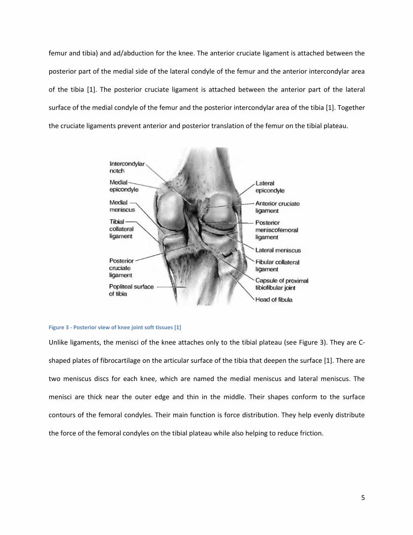
femur and tibia) and ad/abduction for the knee. The anterior cruciate ligament is attached between the

posterior part of the medial side of the lateral condyle of the femur and the anterior intercondylar area

of the tibia [1]. The posterior cruciate ligament is attached between the anterior part of the lateral

surface of the medial condyle of the femur and the posterior intercondylar area of the tibia [1]. Together

the cruciate ligaments prevent anterior and posterior translation of the femur on the tibial plateau.

Figure 3 - Posterior view of knee joint soft tissues [1]

Unlike ligaments, the menisci of the knee attaches only to the tibial plateau (see Figure 3). They are C-

shaped plates of fibrocartilage on the articular surface of the tibia that deepen the surface [1]. There are

two meniscus discs for each knee, which are named the medial meniscus and lateral meniscus. The

menisci are thick near the outer edge and thin in the middle. Their shapes conform to the surface

contours of the femoral condyles. Their main function is force distribution. They help evenly distribute

the force of the femoral condyles on the tibial plateau while also helping to reduce friction.

6

1.2 Knee Joint Biomechanics

The field of knee joint biomechanics refers to the study of the structure and function of the knee. In

order to develop more effective treatments for knee injuries and diseases, it is important to first

understand the kinematics, dynamics, and material properties of the joint. The knee is a crucial

component of a wide range of human activities including the most common form of exercise, walking.

Walking can be defined as a method of locomotion involving the use of the two legs alternately to

provide both support and propulsion, with at least one foot being in contact with the ground at all times

[2]. The study of the biomechanics of walking is called gait analysis.

Gait analysis studies the smallest repetitive period during walking, which is the time between two heel

strikes for the same foot. A gait cycle typically starts at heel strike (0% gait cycle). It has 2 phases: stance

phase and swing phase. Stance phase is the period of time between heel strike and toe off for the same

foot and it accounts for the first 60% of the gait cycle. Swing phase refers to the period when the foot is

not in contact with the ground and it accounts for the other 40% of the cycle.

Due to its position on the lower limb, the knee joint is the focal point of many gait studies [3, 4, 5, 6]. It

is considered a major load bearing joint. The majority of the body's weight and inertia will be felt by the

knee during gait. Pathologies and injuries of the knee can result in decreased mobility as well as pain.

The following sections describe the gait kinematics and dynamics of health knee joint motion.

1.2.1 Kinematics

Kinematics refers to the study of movements. Kinematic analysis of the knee can offer information

about the joint's range of motion, movement profile, and repeatability. Motion of the knee is typically

described in three joint angles: flexion/extension, ab/adduction and in/external rotation (Figure 4).

These joint angles can be measured using a joint coordinate system (JCS). A popular JCS is the Grood and

Suntay coordinate system [7]. This system uses bony landmarks on the femur and tibia to create two

7

frames of reference (one for the femur and another for the tibia) and calculates the angles between

them through vector analysis.

Figure 4 - Illustration of knee joint angles [7]

Studies have reported knee joint angle data (see Figure 5) for various in-vivo activities. A study by

Desloovere 2010 reported joint angles for the knee during walking [6]. The study used 10 adult

volunteers, all without a history of musculoskeletal pathology. The results from this paper showed the

range of motion of the knee during normal walking to be between 2.6 to 64 degrees of flexion, -0.1 to

8.2 degrees of adduction, and -4.2 to 10.2 degrees of internal rotation [6]. Furthermore, the maximum

intra-subject variance of knee joint angles during gait were recorded as 2.7 degrees for knee flexion, 1.6

degrees for ab/adduction and 2.5 degrees for in/external rotation [6].

8

Figure 5 - Knee joint range of motion during gait [8]

1.2.2 Force Analysis

Knee joint force analysis describes the amount of load that the knee experiences during various

activities. Direct measurement of joint contact force in-vivo can be challenging due to its invasive

9

nature, especially from healthy subjects. Much of the data recorded in this area comes from

instrumented knee replacements and 3D computer models.

Factors that contribute to the total knee joint contact force include muscle forces, gravity, and inertia. In

order to calculate joint forces during gait, previous studies [3, 4] have used computer generated

musculoskeletal models. These models have been shown to closely resemble the actual forces recorded

from a patient with total knee replacement [3]. Results from these studies showed similar loading

patterns for the knee. Their data illustrated 2 peaks in the joint contact force during gait. These 2 peaks

occurred roughly around 20% and 50% gait cycle (shortly after heel strike and before toe off), and their

force values were 270% and 200% body weight (Figure 6), respectively [4].

Figure 6 - Knee joint contact force during gait [4]

Joint contact force is the resultant of a variety of component forces, such as gravity, inertia, and muscle

forces. Force component analysis have showed that during gait, muscle forces contribute significantly to

the ground reaction force (GRF), even more than gravity [5]. GRF is one of the main components of knee

joint contact force [4]. Immediately following heel strike, the effects of muscle forces make up almost

90% of the GRF [5]. Similar results can be seen before toe off. During the flat foot section of gait, the

10

flexion angle of the leg is near 0 degrees. It is only during this time that gravity has a more significant

effect on the GRF [5]. This indicates that under peak loading conditions, muscles forces are the primary

contributor to knee joint contact force.

Different muscles are activated at different points in the gait cycles. The Sasaki 2010 paper studied the

individual muscle contributions to knee joint contact force during normal walking [4]. This study used a

computer generated model with 13 functional muscle groups per leg to simulate walking motion [4].

The force profiles for each of the muscle groups were reported as a function of percent gait cycle. Two

peaks in joint contact force were reported per gait cycle. Similar to other studies, these peaks occurred

at roughly 15% and 50% gait cycle, and registered joint forces of up to 280% and 200% body weight,

respectively [4]. The three primary muscle contributors to the joint contact force were the quadriceps,

hamstring and gastrocnemius. Peak forces registered by these muscles were approximately 900N for the

quadriceps, 500N for the hamstring and 700N for the gastrocnemius (Figure 7) [4].

Figure 7 - Muscle forces during gait [4]

11

1.3 Medical Imaging

There are many ways of performing biomechanical analysis on the knee. A method that is commonly

used in research and clinical applications is medical imaging. Medical imaging modalities such as

magnetic resonance imaging (MRI) and computed tomography (CT) are used for non-invasive

examination of knee joint health [9, 10, 11, 12, 13, 14]. These techniques allow assessment of knee joint

health via cartilage thickness measurements [9], or visualization of lesions and/or injuries within the

cartilage, menisci and other soft tissues [11]. MRI is often used to assess the properties of cartilage,

meniscus and other soft tissue structures [11] while CT and high resolution micro CT (µCT) are more

frequently used to study bones and trabecular structures [15, 16]. Co-registration of MR and CT images

can provide a more comprehensive assessment of joint health [11].

1.3.1 Magnetic Resonance Imaging

Magnetic resonance imaging is a medical imaging technique that uses the property of nuclear magnetic

resonance to image nuclei of atoms inside the body [17]. This technology applies a powerful magnetic

field, often 1.5 to 3 Tesla, and measures the radio frequency (RF) signal generated by the body's water

molecules. Tissues with different water density will generate signals of varying strength. These

variations are used to compile a 3D image of the subject.

Due to the nature of MR technology, tissues with higher water content (ligaments, menisci and

cartilage) will generate stronger signals than drier tissues such as bones. Furthermore, since RF signals

are not harmful for the human body, MRI can be used to perform in-vivo biomechanics studies. This

makes MRI a popular research and clinical tool for visualizing soft tissues. Many previous studies have

used MR technology to analyze knee joint cartilage topography, thickness and contact area [18, 9, 11].

More recently, open dynamics MRI technology has been used to study the mechanics of knee joint

12

movement [10]. These studies can offer much insight into the inner workings of the knee, which can

help future patients to prolong joint health as well as more effectively prevent and treat injuries.

When performing research with MR scanners, certain safety considerations must be made. Due to the

strength of the magnetic field required to generate a measurable signal, all ferromagnetic materials,

such as iron, steel, nickel, etc., are not permitted in the room. Non ferromagnetic metals, such as

aluminum, brass and copper, can be considered safe in certain low powered MR facilities; however, they

will still generate interference in the imaging process. All metallic objects will to some degree generate

MR artefacts and distort the MR image. For this reason, metallic objects should be kept a certain

distance away from the imaging zone. This distance depends on the shape and composition of the

material. These MR properties play an important role in the design of any MR compatible devices.

1.3.2 Micro Computed Tomography

Micro computed tomography is an imaging technique that is not entirely limited to the biomedical field.

It uses X-rays to create cross sections of 3D objects that later can be used to assemble a virtual model.

This technology is based on the measurement of X-ray attenuations as they pass through various

objects. X-ray, unlike MR radio signal, is a type of ionizing radiation. The amount of X-ray absorption is

related to tissue density: bone absorbs the most and soft tissues absorb much less [19]. This makes µCT

scans very effective at imaging bones. However, since X-ray can be harmful to the human body, duration

of exposure to patients and subjects must be closely monitored.

µCT images have been used to compare trabecular structures of patients suffering from various illnesses

[16]. These images provide researchers with quantifiable parameters such as bone volume fraction,

trabecular thickness, number and separation [16, 15]. These parameters can be used to study stiffness,

strain and stress distribution within the bone. CT can also be used to collect subject specific geometrical

data of joints such as the knee [13]. This type of information can be used by clinicians to address pain

13

after joint replacement surgeries [13]. It can also be used by manufacturers to improve and customize

implant designs [13].

1.4 In-vitro Joint Testing

Another method of studying knee joint biomechanics is through the use of cadaver joints. In-vitro knee

joint studies can provide data such as pressure distribution of various joint implants [20], effects of

different muscle loading scenarios [21, 22], or the effects of specific injuries or surgical procedures on

joint kinematics [23]. There are many benefits to in-vitro studies when compared with in-vivo. Joint load

application is much easier to control. An accurate and repeatable force can be applied to a specific

muscle or bone in a repetitive manner. This is often not possible with live subjects. It is also easier to

perform well controlled assessments to characterize the effect of tissue injury and repair. It should be

noted, however, that load application to a cadaver knee joint may not be entirely physiological due to

the absence of certain active muscle loads. Many loading simulators are designed to replicate in-vivo

conditions with varying degrees of success. Popular designs are discussed in the following sections.

In-vitro biomechanical testing can also be used in conjunction with medical imaging techniques. This

combination has been used in many experiments to study outcome measurements such as joint

load/displacement response [24], cartilage displacement and strain patterns [25], and cartilage

thickness mapping [26]. Since medical imaging is a non-invasive method of data collection, its

combination with in-vitro testing provides a closer representation of in-vivo conditions. In order to

facilitate these types of experiments, various knee joint loading simulators were built. These devices are

described in detail in the following sections.

1.4.1 Imaging Compatible Knee Joint Loading Apparatus

The Martin 2009 paper describes a MR compatible device used to study the quasi-steady-state

displacement response of human cadaveric knee joints [24]. This device is designed to be MR

14

compatible and capable of inducing cyclic compressive loading. The device is driven by a pressure

controlled pneumatic cylinder with a maximum force output of 1500N. Joint force is applied via the

tibia. The cylinder is attached to the distal end of the tibia on the cadaver knee through a four-degree of

freedom attachment device. The femur end of the knee joint is locked in a clamp used to set the flexion

angle. The device is made entirely from wood, plastic, aluminum and stainless steel, which makes it MR

safe.

The Chan 2009 paper described a MR compatible device that can apply cyclic compressive loads to

porcine knee joints [25]. The loading device was designed to fit within a 7.0T MR scanner. It is made

entirely of plastic and non-ferromagnetic metals. No metals components were located within the RF coil

to minimize artefacts. Load was applied using a computer controlled double acting pneumatic cylinder

directly to the ends of the tibia and femur. This device restricted every DOF for the knee except

compression-distraction.

The Song 2006 paper described a MR compatible device that applied compressive loads to sheep knee

joints [26]. This loading system consisted of a cylindrical shaped MR compatible container lined with a

pneumatically actuated air bladder. This device was designed to apply uniaxial compressive loads in a

4.7T MR scanner. It was also designed to allow X-ray transmission in case µCT scans were required. The

sheep knee was frozen at 45° and a 4.5cm cross section of the joint was drilled out using a circle saw.

This cross section is then thawed and inserted into the loading cylinder. Compressive load was applied

through the air bladder and controlled with custom electronics.

These devices share a few common traits. Loads were all applied axially through the femur and tibia. No

muscle forces were considered and freedom for the knee joint movement was restricted in all designs. It

is debatable if this type of loading represents the load seen physiologically. Without the application of

quadriceps loads to counterbalance flexion moments about the knee, it is impossible to reach static

15

equilibrium in flexed positions with six DOF. For this reason, all loading systems described above

restricted at least one DOF for the knee. Since the knee has six DOF in-vivo, these restrictions introduce

physiological inaccuracies. Also, as mentioned in previous sections, muscle forces contribute significantly

to joint contact force and stability. Studies have shown the application of quadriceps and hamstring

loads changes the kinematics of knee joint motion [21]. By excluding muscle forces, these designs are

not applying loads in a physiologically relevant manner. It has also been shown in previous studies that

active muscle simulation generates more repeatable joint angles than passive simulation (loads applied

directly to the bones through axial compression) [27, 28]. In research applications requiring high levels

of joint angle repeatability, such as cartilage contact area and meniscal movement analysis, muscle

forces may be an optimal method of attempting to replicate physiologic loading.

1.4.2 Non Imaging Compatible Knee Joint Loading Apparatus

Muscle simulation and six DOF loading for in-vitro knee joints have been incorporated in certain non

imaging compatible loading systems. One of such systems commonly used by researchers is called the

Oxford Rig [21, 23, 29]. Figure 8 shows an overview of the Oxford rig. This rig is capable of applying hip,

quadriceps and hamstring loads to a cadaver knee joint. The hip end of the knee is attached to a slider.

This allows adjustments to hip height and knee flexion angle. By counterbalancing the hip loads with

quadriceps loads, the rig is capable of maintaining the knee in any flexion angle [30]. This simulates real

life knee loading during activities such as squatting [23].

Another key feature of the Oxford rig is that it allows all possible anatomical movements for the knee.

Its design offers six DOF for the knee [30]. The two rotations at the hip and three rotations at the ankle

act like a pair of ball and socket joints, and the slider allows hip height to change as the knee flexes [30].

By having these degrees of freedom, the rig avoids preloading the knee and it does not restrict motion

of the joint.

16

Figure 8 - Overview of the Oxford rig [23]

By simulating quadriceps and hamstring loads, the Oxford rig offers a more physiological and repeatable

way of applying loads to the knee. However, its size and composition makes it incompatible with

imaging modalities such as MRI and CT. The bore of the MR and CT scanners are much smaller than the

dimensions of the rig. In addition, MR compatibility requires the device to be free of ferromagnetic

metals. Since the Oxford rig is typically built with steel, it is not MR safe.

1.5 Problem Statement and Objective

A device that allows repeatable positioning and physiologic loading of a cadaveric knee joint while

maintaining compatibility with imaging modalities such as MRI and CT would be valuable for assessment

17

of knee joint biomechanics. Such a device would permit laboratory based experimental testing that

could validate computational knee joint models, as well as address the efficacy of established and

evolving ligament, soft tissue and bone repair methods. As mentioned in previous sections, existing

MR/CT compatible knee joint loading devices do not simulate muscle forces and offer limited DOF for

the knee. This type of loading is expected to be less repeatable than muscle force simulation and less

physiologic in nature. For in-vitro studies in which cartilage contact area or meniscal movement is a

desired outcome measure, physiologic loading is essential. The objective of this thesis is to describe the

design of a MR and µCT compatible device that is capable of applying physiologically relevant muscle

forces to intact cadaveric knee joints at various flexion angles with high levels of precision. Moreover,

the device must be able to replicate the knee joint's kinematics and dynamics during gait and function

within MR and µCT scanners without creating imaging artefacts. Detailed specifications related to the

design constraints for this device are described in the following chapter.

18

2 MR/µCT Compatible Cadaver Knee Joint Loading Device Design

Chapter 2 describes the specifications and design details of a MR/µCT compatible knee joint loading

simulator.

2.1 Design Specifications

Specifications for the loading device (summarized in Table 1) are derived from the kinematics and

dynamics data discussed in Section 1.2.

The range of motion of the loading device must encompass the entire knee joint flexion angle range

seen during gait, which is approximately 0 to 60 degrees (Section 1.2.1).

The device must offer six DOF for the knee and be able to load and position the joint with

repeatability equal to or better than the intra-subject repeatability of gait kinematics [6].

The available force output of the device must be greater than the in-vivo peak muscle forces seen

during gait, which were 900N for the quadriceps and 500N for the hamstring (Section 1.2.2).

The loading platform must fit within MR and µCT scanners. Since µCT scanners typically have smaller

bore diameters than MR scanners, the critical dimension for the loading device is the bore size of

the µCT scanner selected for testing (27cm). The device must be compatible with this dimension.

The device must also be safe to operate within 1.5T MR scanners and not introduce artefacts in the

resultant scans.

Table 1 - Design specifications for the MR/CT compatible knee joint loading device

Parameters Values

Flexion Angle Range 0 to 60 degrees

Joint Angle Precision Within intra-subject gait variation [6]

Quadriceps Force > 900 N (see Section 1.2.2)

19

Hamstring Force > 500 N (see Section 1.2.2)

Dimension Fit into 27 cm diameter µCT bore

MR Compatibility No MR artefacts within 1.5T scanners

Degrees of Freedom 6 degrees of freedom for the knee

2.2 System Overview

In order to meet the design specifications listed above, the loading device was divided into three main

subsystems: loading platform, hydraulic control unit and automation controls. Since the automation

controls and hydraulic control unit are not MR safe, they are located separately from the loading

platform where the cadaver knee will be installed. The loading platform is entirely compatible with 1.5T

MR scanners and has a cross section that fits within a 27cm bore. To ensure MR safety, all hardware

except the loading platform is place outside the MR room. The platform is connected to the control

systems through shielded wires and rubber hydraulic hoses. Figure 9 shows the schematics for the

overall system. Pictures of subsystems can be found in Figure 20 of Appendix A.

The platform uses hydraulic cylinders to set flexion angles and apply quadriceps and hamstring forces.

The effects of the gastrocnemius are not considered in this design due to space constraints. The loading

platform includes three hydraulic cylinders, two custom made uniaxial load cells and a six DOF titanium

load cell. The hydraulic cylinders on the platform are powered by the hydraulic control unit. They are

connected through six rubber hydraulic hoses. The uniaxial load cells record tensile forces from

individual muscle cables. They are connected to a data acquisition system through shielded wires. The

six DOF load cell is used to record joint contact force. It is connected to a separate data acquisition

system through shielded wires.

20

The automation of this loading system is programmed and controlled using a laptop equipped with

LabVIEW. The laptop receives signals from both of the data acquisition systems. These signals are

processed using a custom written program and outputs are sent to the automation control board. This

board acts as an interface between the laptop and the hydraulic control unit. Details of automation

design are discussed in Section 2.10.

Figure 9 - Overall system schematics for the MR/µCT compatible knee joint loading device. Three main subsystems are shown: loading platform, hydraulic control unit and automation controls. Automation controls include load cell DAQ, strain gauge DAQ, output module, automation control board and laptop.

2.3 Material Selection

Due to the magnetic properties of MR scanners, ferromagnetic materials cannot be used in the loading

platform. Plastics are the most MR compatible. Metals such as steel, nickel, etc. are safety hazards

within the scanner. Certain non-ferromagnetic metals such as copper and brass are safe within low

MR Compatible Loading Platform

Hydraulic Control Unit

Load Cell DAQ

Strain Gauge DAQ

Laptop

Output Module

Automation Control Board

Inside MR Room

Outside MR Room

21

power MR scanners; however, they still generate susceptibility artefacts in MR images. A preliminary

experiment was conducted to test the susceptibility of various MR safe metals.

Five types of non-ferromagnetic metals were tested, which included brass, copper, aluminum, Monel

and 304 stainless steel. Each metal was first placed next to a small rare earth magnet to confirm MR

safety. Stainless steel showed a small reaction to the magnet and was removed from further testing. The

remaining four metal parts were secured to a length of plastic pipe and immersed in a container filled

with a MR contrast agent (water with gadolinium). This container was scanned and the resulting image

was analyzed (see Figure 10). It was observed that brass, copper and aluminum caused minimal

artefacts outside of a radius of a few centimeters, while Monel caused significant artefacts throughout

the container. Based on these results, the design of the loading platform was limited to plastics, brass,

copper and aluminum.

Figure 10 - Magnetic resonance scans of building materials.

Brass Nut Aluminum Bolt

Copper Crimp Monel Wire Rope

22

2.4 Loading Platform Structure and Geometry

The frame of the loading platform (Figure 11) is designed to accommodate three hydraulic cylinders and

a cadaver knee joint. This is accomplished through the use of an elongated structure. The cadaver knee

joint is installed in the middle section of the platform while the hydraulic cylinders are mounted on both

ends. The quadriceps and hamstring cylinders are mounted on the femoral end of the platform and the

cylinder used to set flexion angles is mounted on the tibial end. The overall length of the platform is

1.8m. The height of the platform is 16cm and the width is 20cm at its widest point. This allows the

platform to fit longitudinally in a 27cm diameter µCT scanner.

Two 1.8m (6') lengths of fibreglass rails with cross sections of 12.7mm x 101.6mm (1/2" x 4") are the

main structural components of the platform. Fibreglass was chosen for its structural strength. The rails

act as the bottom and top mounting plates for the platform. They are attached to each other through

five aluminum support plates and two polycarbonate panels. Two of the aluminum support plates also

act as hydraulic cylinder mounts. The polycarbonate panels are attached to the sides of the middle

section of the platform. The middle section employs an open top design. This accommodates higher

flexion angles for the knee. It also makes joint installation much easier to perform.

Figure 11 - Structural components of the loading platform. Highlighted rectangle (red) represents the load carrying zone.

Fibreglass Rails

Aluminum Support Plates

Polycarbonate Panels

23

Load on the cadaver knee joint is applied by the retraction of the quadriceps and hamstring cylinders.

This retraction exerts a pull force on the tibia of the joint through two muscle cables. The resultant joint

force is transmitted to the frame of the platform through a pin joint that is attached to an aluminum

support plate. The area between this support plate and the hydraulic cylinder mounting plate is known

as the load carrying zone (Figure 11). This area of the platform sees the majority of the compressive

force generated by the cylinders. The main structural components in the load carrying zone are the two

fibreglass rails. Assuming each cylinder can generate a maximum force output of 1400N (see Section 2.5

below) and an even force distribution among the two rails, the compressive stress in the fibreglass rails

were calculated to be 3.03MPa (440PSI). Specifications from the manufacturer indicated the

compressive strength of the fibreglass rails to be between 96.5 and 483MPa (14000 and 70000PSI).

Based on this data, the compressive stress caused by the hydraulic cylinders is far below the structural

capability of the frame.

2.5 Actuators

Three types of actuators were considered for the loading platform, including electric motors, pneumatic

cylinders, and hydraulic cylinders. Motors were quickly eliminated as a possible option due to their

magnetic properties. Motors cannot be placed within the MR room, and the construction of a

transmission system that can accommodate motors from outside the MR room was deemed impractical.

Pneumatic and hydraulic cylinders can both be modified to be MR safe. Pneumatic cylinders are usually

faster but less stable since air is a compressible fluid. Hydraulic cylinders are more stable and precise,

but their response time is slower. Since the application required precision over speed, hydraulic

cylinders were chosen as the desired actuators.

The loading platform consists of three hydraulic cylinders. Two are used to simulate quadriceps and

hamstring forces. One is used to translate the tibial end of cadaver knees for the purpose of setting

24

flexion angles. According to the specifications, the quadriceps and hamstring cylinders must be capable

of outputting 900N and 500N of force, respectively. Assuming the hydraulic pump has a maximum

output pressure of 1.38Mpa (200PSI), the following sizing calculations were made for the cylinders.

Since muscle forces are simulated with cylinder retractions, the cross sectional area of the cylinder rod

has to be incorporated (standard rod radius is 6.35mm or 1/4").

P = 1.38MPa Fq = 900N Fh = 500N Rrod = 6.35mm

Based on these calculations, the bore size for the quadriceps and hamstring cylinders must be greater

than 31.5mm and 25mm, respectively. For design simplicity and parts availability, all hydraulic cylinders

were sized with a bore diameter of 38mm (1.5in). Hydraulic cylinders of this size is capable of generating

a maximum retraction force of approximately 1400N. The stroke length of the cylinders were chosen

based on the size constraint of the platform. The framing materials were available in lengths of 1.8m,

which limited the overall length of the platform. Based on this dimension, an appropriate stroke length

was determined to be 102mm (4in).

25

Three brass hydraulic cylinders with 38mm (1.5in) diameter bore and 102mm (4in) stroke length were

purchased (Allenair brass cylinder, type E configuration). These off the shelf cylinders included a few

stainless steel parts, which had to be replaced with brass, copper, or aluminum. The stainless steel

cylinder rod was replaced by a custom machined aluminum rod. The stainless steel locknut on the piston

was replaced with a brass nut with identical threads. The stainless steel retaining rings at the ends of the

cylinders were replaced with copper retaining rings. After these modifications were made, the hydraulic

cylinders were scanned in a 1.5T MR facility to ensure compatibility.

2.6 Degrees of freedom

The knee joint in vivo has six DOF. In order to replicate physiological loading conditions, the loading

platform also offers six DOF. Two custom designed plastic bone pots act as the interface between the

cadaver knee joint and the loading platform. The pots are of cylindrical shape and made from 51mm (2")

ABS piping and caps. The proximal end of the femur and distal end of the tibia are secured in the pots

with three brass screws and quick drying dental cement (Instant Tray Mix Powder, Lang Dental

Manufacturing Corporation). The six DOF load cell (Model 30E15, JR3 Inc., see Figure 12) used to

measure joint forces is mounted on the femoral pot in line with the axis of the femur. This load cell

attaches to the platform frame through a pin joint. The distal tibial pot attaches directly to the distal

hydraulic cylinder through a rod end ball joint. This design offers freedom of flexion/extension for the

proximal end of the femur via the pin joint, and three degrees of rotational freedom via the rod end ball

joint, as well as two degrees of translational freedom (medial/lateral and controlled proximal/distal) for

the distal end of the tibia, resulting in six DOF for the knee.

26

Figure 12 - Six DOF MR compatible load cell

2.7 Principle of Operation

This section describes the knee joint installation and load application procedures. During installation, the

femoral load cell is connected to the platform frame through a 19mm (3/4") diameter aluminum pin and

the tibial pot is connected to the distal hydraulic cylinder through another aluminum pin. After securing

the pots, the muscle cables attached to the tibia are fed through a system of pulleys and attached to the

quadriceps and hamstring cylinders. When these cylinders retract, tension is generated in the cables

simulating muscle tension. The line of action of the muscle cables are carefully maintained by two brass

eye screws mounted on the femoral pot and a plastic cable tie that's attached to the patella.

Once the cadaver knee is installed in the loading platform, the loading process is initiated by manually

actuating the distal hydraulic cylinder to set the flexion angle. The position of this cylinder is measure

with a scale mounted on the platform frame (Figure 13). This scale allows the operator to repeat flexion

angles with high levels of precision. Once the desired angle is achieved, joint load is applied via

alternating force increments on the quadriceps and hamstrings cylinders. The two custom built uniaxial

load cells, mounted on the clevises at the ends of the quadriceps and hamstring cylinder rods, provide

real time force feedback. The force application process is automated using a laptop running a custom

27

written LabVIEW program. This program monitors the strain gauge signals and incrementally retracts

the quadriceps and hamstring cylinders until the desired force is reached on both. Details of the

automation program can be found in Section 2.10.

Figure 13 - Scale used for measuring flexion angles (highlighted in red)

2.8 Hydraulic Control Unit

The hydraulic control unit consists of the pump and valves that are required to power the hydraulic

cylinders on the loading platform (Figure 14). The chosen hydraulic pump (108 AE S 10-C NN-3 V-02-02,

Parker Hannifin Corp) is capable of outputting a maximum pressure of 1.38MPa (200PSI) and a nominal

flow rate of 6.55x10-4 m3/min (40cipm). Flow rate from the pump is directly related to the movement

speed of the cylinders. In order to achieve high load precision, the loading speed should be kept low. For

this reason, an affordable pump with the lowest nominal flow rate was chosen. A four way three

position solenoid valve (SWH-G02-C2-A120-10, Northman Fluid Power) is used to control the movement

direction of the cylinders. Six normally closed solenoid valves (7121KBN2NR00N0C111P3, Parker

Hannifin Corp) are used to control cylinder activation. Schematics of the hydraulic circuit is shown in

28

Figure 21, Appendix A. The hydraulic pump is powered by a 12VDC/20A power supply (Phoenix Contact,

QUINT-PS/ 1AC/12DC/20). The solenoid valves are powered by 120VAC.

Figure 14 - Hydraulic control unit

The hydraulic circuit can be controlled both manually or with automation. Manual controls are located

on the electrical box of the hydraulic control unit. They include four toggle switches and two push

buttons. One of the toggle switches activates the hydraulic pump, while the other three are used to

select hydraulic cylinders (i.e. if the quadriceps toggle switch is on when flow is activated, then the

quadriceps cylinder will move). The two push buttons are used to control the movement direction of the

cylinders. One button instructs the cylinders to extend and the other to retract. Automation programs

can also be used to control this circuit. This method of control is discussed in detail in Section 2.10.

On/Off

Solenoid Valves

4 Way 3 Position

Solenoid Valve

Hydraulic PumpElectrical Box and

Power Supply

29

2.9 Special Considerations for MR Setup

As previously mentioned, the hydraulic control unit and automation hardware are not MR safe. For this

reason, when setting up the loading platform in MR facilities, it is very important to keep the control

systems out of the MR room. The loading platform should be the only piece of equipment to be placed

inside the scanner. Rubber hydraulic hoses stemming from the platform are connected to the hydraulic

control unit through the walls of the MR room. Shielded cables from the load cell and strain gauges,

however, are routed through a different interface.

MR scanners are susceptible to many forms of electromagnetic interference. The presence of electronic

cables and sensors can introduce large amounts of interference in MR images, which was observed

during preliminary trials. These interferences were likely caused by the shielded cables. During

preliminary trials, cables were routed through the wall in a similar fashion to the hydraulic hoses. It was

determined that these cables carried outside noises into the MR room and caused the artefacts in the

images. Typically, MR facilities have wave guide systems that filter out these types of noises. After the

preliminary trials, the loading platform sensors were modified to be compatible with the wave guide

interface. The subsequent scans showed significantly less interference and this setup is strongly

encouraged in future tests.

2.10 Automation of Knee Joint Loading Process

The hydraulic circuit for the loading platform can be controlled either manually or with automation.

Manual control offers flexibility in terms of real time load adjustments; however, it is prone to human

error and is very much operator dependent. When operated by different people, the applied joint load

can vary greatly. Since this loading device is intended as a tool for multiple research applications,

operator bias becomes a serious issue. To address this, an automated loading protocol was developed.

30

Loading automation is controlled by a laptop equipped with LabVIEW software. A custom written

LabVIEW program is used to process sensor inputs from the loading platform and output control signals

to the hydraulic control unit. In order to individually control the quadriceps and hamstring cylinders, two

uniaxial load cells were constructed using strain gauges and mounted on the cylinder rods. These load

cells allow the automation program to apply varying ratios of quadriceps/hamstring forces. The

hardware and software details of these automation features are discussed in the following sections.

2.10.1 Input Hardware

There are three sensors on the loading platform: two uniaxial load cells and a six DOF load cell. The

uniaxial load cells were custom made by mounting strain gauges (Vishay EA-06-125TG-350 dual element

90º TEE rosette, Intertechnology Inc.) on the bottom surface of the aluminum clevis at the ends of the

quadriceps and hamstring cylinder rods (see Figure 15). This clevis was designed to exert a bending

moment on its bottom surface during tension. When a force of 660N (150lb) is applied to the clevis in

tension, this surface will register approximately 400 micro-strain. This level of deformation generates a

measurable signal for the strain gauges.

The strain gauges are of TEE rosette construction, which means each gauge has two active elements

oriented at 90° with respect to each other. The TEE rosette is ideal for use in half bridge circuits. When

compared with quarter bridge circuits, half bridge circuits offer benefits such as temperature

compensation and additional signal strength. Figure 16A shows the circuit diagram for the uniaxial load

cell. R1 and R2 are completion resistors. They are located within the strain gauge data acquisition

system (NI SCXI 1314, National Instruments) along with the voltage supply. R3 and R4 are active gauge

elements on the loading platform. Signals from these elements are measured by the data acquisition

system and sent to the processing laptop via USB connection. The uniaxial load cells were calibrated

31

(Figure 16B) on an Instron materials testing machine (Model 5965) and found to be linear with an R2

value of 0.99 and repeatable with an average standard deviation (SD) of 0.64% over four repeated trials.

Figure 15 - Uniaxial load cell design. All dimensions are in inches

Figure 16 - A: Half bridge circuit diagram. B: Instron calibration of uniaxial load cell

Strain Gauge Attachment Surface

A B

32

Unlike the uniaxial load cells, which are used to measure individual muscle forces, the six DOF load cell is

used to measure resultant force on the joint. This load cell is a commercially available MR compatible

device. It is positioned in line with the femur of the cadaver knee joint and it records joint contact force.

It is connected to a separate data acquisition system (NI 9205, National Instruments) through shielded

wires. It generates six signals, which represents forces and moments about the three Cartesian axis.

Data from this load cell is used as an outcome measure of loading experiments.

2.10.2 Output Hardware

In order to activate the hydraulic cylinders on the loading platform through automation, a signal output

system was designed to interface the processing laptop with the hydraulic control unit. The laptop

outputs commands through an USB connection to a four channel output module (NI 9263, National

Instruments). This module converts the on/off commands from the laptop into a 12V signal. The

maximum power output for this module is 12VDC and 10mA. The hydraulic solenoids, on the other

hand, require 120VAC. In order to match up the power requirements, an interface circuit (the

automation control board) was constructed.

The automation control board separates the power supply for the hydraulics (located in the hydraulic

control unit) from the output module through the use of relays (see Figure 22 in Appendix A). This circuit

board has its own 12VDC power supply. It receives four 12V inputs from the output module. These

inputs represent commands to the quadriceps and hamstring cylinders, as well as the solenoids that

control their direction of movement (i.e. extend/retract). The 12V signal from the output module

activates a MOSFET (metal-oxide-semiconductor field-effect transistor) circuit that triggers a coil relay.

The contact side of the relay is connected to the hydraulic control unit. By closing the contacts, a

solenoid is activated. Since no current can pass between the coil of a relay and its contacts, the output

module is completely isolated from the hydraulic control board.

33

2.10.3 Software

The processing laptop uses a custom written LabVIEW program (version 8.5) to control the automation

of the loading process. This program accepts inputs from the sensors on the loading platform and

outputs commands to the hydraulic control unit. There are three inputs and four outputs. Inputs include

the signals from the uniaxial load cells and the six DOF load cell. Outputs include the triggers for the

solenoids controlling the extension and retraction of the quadriceps and hamstring cylinders. Figure 23

in Appendix A shows an overview of the program. The entire program is structured within a

synchronized "while" loop, where every loop has a duration of 100ms.

The program can be divided into six sections (Figure 23). Section 1 is responsible for receiving signals

from the uniaxial load cells. Signal from the strain gauge data acquisition system is sampled at 50Hz (five

times per loop). The sampled signal is then divided into two separate strain readings, one for the

quadriceps and the other for the hamstring. Each strain reading has five sample points per loop. These

five sample points are averaged and the resultant values are sent to a real time Butterworth low pass

filter in section 2.

Data recorded from preliminary MR trials showed significant noises in the strain gauge output. This

noise was generated by the alternating magnetic field of the scanner during operation. This MR noise

had an approximate frequency of 2 - 3Hz. A second order Butterworth low pass filter with a cut-off

frequency of 1.5Hz was used for real time noise reduction. The code for this filter can be found in

section 2. Second order Butterworth filters require two past sample points. For this reason, a double

shift register was added in the "while" loop. The output of the Butterworth filter is sent to the graphing

function in section 3 and the load control function in section 5.

The code from section 3 is responsible for the output of the filtered strain readings. These readings are

outputted in two formats. They are displayed in real time on the user interface with a graphing function

34

and also saved in a text file. The code from section 4 is responsible for receiving the force and moment

signals from the six DOF load cell. Data from this load cell is sampled at 20Hz (twice per loop). The raw

voltage measured from the load cell is multiplied by a calibration matrix and transformed into force and

moment readings. These readings are then displayed in real time on the user interface with a graphing

function. Unlike the uniaxial load cells, signals from the six DOF load cell did not experience the same

MR interference during preliminary trials, and were therefore not filtered.

Once all sensor inputs have been properly conditioned, they are sent to the load control function for

processing. The load control function is located in section 5. It is the primary control algorithm for the

hydraulics automation. This algorithm uses inputs from the sensors as well as the user interface to

determine the proper outputs to send to the hydraulic control unit. There are three main versions of this

algorithm, each with a different loading profile. These profiles are described below.

2.10.3.1 Loading Profiles

A loading profile defines to the way load is applied to a cadaver knee joint. Different research

applications may require different muscle activation patterns. Three different loading profiles were

programmed to accommodate a wide range of possible applications. The design of these loading profiles

as well as their benefits and drawbacks are discussed in the following sections.

2.10.3.1.1 Continuous

The simplest loading profile for applying muscle forces is continuous activation analogous to isotonic

contraction of the muscles around the knee. With this profile, the operator inputs two desired force

levels, one for the quadriceps and another for the hamstrings. The program will then activate the

quadriceps and hamstring cylinders continuously and simultaneously until the desired force level is

reach on both.

35

This method of load application offers the fastest possible loading speed. The speed of muscle

activation resembles in-vivo muscle activities during normal gait. It is, however, low in accuracy and

repeatability. The current hardware can only provide one speed for hydraulic activation. This means that

there is no way of slowing down the quadriceps and hamstring cylinders as the desired force level is

approached. For this reason, a continuous loading profile results in a significant amount of load

overshoot (up to 200N). This becomes a problem for research applications where load repeatability is

crucial.

2.10.3.1.2 Cyclic

Certain fields of research, such as cartilage studies, may require a dynamic or cyclic loading scenario. For

this reason, a cyclic loading profile was developed. With this profile, the user inputs two desired force

levels, one for the quadriceps and another for the hamstring. The program will load the cadaver knee

joint to the desired force level and unload it immediately after. This process is then repeated

continuously until it is stopped by the user. The single cycle load application process in this profile is

identical to that of the continuous loading profile.

Since the continuous loading profile is used for every cycle, the cyclic loading profile will experience

similar drawbacks. The accuracy and repeatability of the applied load is low; however, preliminary data

shows the timing repeatability of this profile to be within +/- 0.1 seconds. This profile may potentially

be useful in dynamic imaging applications, where the timing of load application is crucial.

2.10.3.1.3 Incremental

For research applications where load repeatability is important, an incremental loading profile was

developed to reduce force overshoot. With this loading profile, the user inputs two desired force levels,

one for the quadriceps and another for the hamstring. The program will then alternately activate the

quadriceps and hamstring cylinders in small bumps (0.1 sec per bump). There is a rest period

36

programmed in between bumps to compensate for the latency of the sensor processing functions. This

process is continued until the desired muscle force levels are reached.

This loading profile has better load accuracy and repeatability than the continuous profile. The

maximum overshoot observed from this profile was approximately 50N. However, due to the addition of

the rest periods in between hydraulic activations, the duration of the loading process is prolonged

significantly. The application of 350N of quadriceps and hamstring load takes approximately 10 seconds.

This loading speed is below that of in-vivo muscle activation. This profile is therefore not recommended

for gait related studies where the speed of muscle activation needs to be physiologically relevant.

2.11 Loading Device Design Discussion

The device described in this chapter meets all design specifications listed in Section 2.1. The loading

platform is made entirely from plastics and non-ferromagnetic metals. This composition is proven to be

compatible with 1.5T MR scanners. To avoid generating susceptibility artefacts in the images, the

section of the platform that houses the cadaver knee joint is completely metal free. Special

considerations have also been made to ensure the sensors on the platform introduce minimal

interference into the MR images.

The frame of the platform is capable of withstanding much higher compressive stress than the output

capacity of the hydraulic cylinders, making it structurally stable. By using an elongated structure, the

cross-sectional area of the loading platform is limited to 16cm x 20cm at its widest points. This allows

the platform to fit within a 27cm diameter bore, which makes it physically compatible with the selected

µCT scanner.

The stroke length of the distal hydraulic cylinder is 102mm (4in), which means the distal end of the tibial

bone pot on the cadaver knee joint is capable of 102mm (4in) of translation in the proximal direction

starting from full extension. The overall length for the cadaver knee joint including bone pots is

37

approximately 560mm (22in). Simplified flexion angle calculations (see Figure 17) show the maximum

flexion angle generated by the platform to be 70 degrees (180 - 110). This accommodates the entire

knee joint range of motion seen during gait (0 to 60 degrees of flexion).

Figure 17 - Knee joint flexion angle calculations

The quadriceps and hamstring cylinders have maximum force outputs of much greater than 900N and

500N, respectively. Due to the hydraulic cylinders being oversized, the maximum retraction force (at

1.38MPa) from each cylinder is approximately 1400N. This additional output capacity allows the loading

platform to meet its force requirements even after frictional losses.

The simulation of muscle forces allows the loading platform to maintain six DOF for the knee joint during

loading. Custom designed bone pots offer one DOF (flexion/extension) on the femoral end and five DOF

(three rotations, medial/lateral translation, and controlled proximal/distal translation) on the tibial end,

which results in six DOF movement for the knee. Validation experiments were performed to measure

the repeatability and reproducibility of the device. Results showed the device to be more repeatable

than the intra-subject variability of gait kinematics. Details of the validation experiments are discussed in

Chapter 3.

280mm 280mm

280mm 280mm

102mm

110 deg

38

3 Design and Validation of Cadaveric Knee Joint Loading Device

Compatible With Magnetic Resonance Imaging and Computed

Tomography

The following chapter is a manuscript that is submitted to the Journal of Orthopaedic Research.

3.1 Introduction

Medical imaging modalities such as magnetic resonance imaging (MRI) and computed tomography (CT)

are used for non-invasive examination of knee joint health [14, 10, 9, 11, 12, 13]. These techniques allow

assessment of knee joint health via cartilage thickness measurements [9], or visualization of lesions

and/or injuries within the cartilage, menisci, bone and other soft tissues [11]. Medical imaging used in

conjunction with in-vitro biomechanical testing has advanced our comprehension of knee joint function

[31, 18]. A device that allows repeatable positioning and loading of a cadaveric knee joint while

maintaining compatibility with both imaging modalities would be valuable for assessment of knee joint

biomechanics. Such a device would permit laboratory based experimental testing that could validate

computational knee joint models, as well as address the efficacy of established and evolving ligament,

soft tissue and bone repair methods.

Existing MR/CT compatible knee joint loading devices [26, 25, 24] do not simulate muscle forces. These

devices apply loads to cadaver knee joints through passive simulations (axial compression of the tibia

against the femur). For passive simulations to reach static equilibrium in flexed positions, the knee joint

cannot have six degrees of freedom (DOF). Therefore, these devices are designed to work only at full

extension [25], or with restricted DOF for the knee [26, 24]. Certain knee joint loading devices, such as

the Oxford rig, offer six DOF and muscle simulation but have not be adapted for imaging [29, 21]. This

type of loading is expected to be more repeatable than passive simulation [27, 28] and more physiologic

in nature [29, 21]. For in-vitro work in which cartilage contact area or meniscal movement is a desired

39

outcome measure, more physiologic loading is essential. The purpose of this paper is to describe a MR

and CT compatible device that is capable of applying physiologically relevant muscle forces to intact

cadaveric knee joints at various flexion angles with high levels of precision. Moreover, the device was

designed to function within MR and CT scanners without creating imaging artefacts.

3.2 Materials and Methods

3.2.1 Knee Joint Loading Device Design

The loading device consists of three hydraulic actuators for positioning the joint and applying muscle

forces. The device has two main sections, the loading platform and the hydraulic control unit. The

loading platform houses and applies loads to cadaveric knee joints. This platform is made of MR safe

materials including fiberglass, plastics and non-ferrous metals such as copper, aluminum and brass. The

hydraulic control unit consists of the pump and valves required to power the loading platform. This

control unit is positioned outside the MR room and connected to the loading platform via rubber

hydraulic hoses.

Details of the loading platform are shown in Figure 18. Cadaveric joints were potted (described below in

specimen preparation) and installed into the middle section of the platform (Figure 18B). The proximal

femoral pot was attached to the platform frame with a pin joint (1DOF – flexion/extension). The distal

tibial pot was attached to the distal hydraulic cylinder (Figure 18A) with a rod end ball joint. This

attachment incorporated three degrees of rotational freedom as well as two degrees of translational

freedom (medial/lateral and controlled proximal/distal) for the distal end of the tibia, resulting in six

DOF for the knee. A six DOF MR compatible load cell (Model 30E15, JR3 Inc.) was placed in-line with the

femur (Figure 18A). In order to simulate muscle forces, cables attached to the tibia (described below in

specimen preparation) were fed through a system of pulleys and attached to two hydraulic cylinders

(Figure 18A). When these cylinders retracted, tension was generated in the cables simulating muscle

40

tension. The lines of action of these cables were maintained with carefully placed eyehole screws, to

replicate the line of action of the muscles [32].

Once the cadaver knee was installed in the loading platform, the loading process was initiated by

actuating the distal hydraulic cylinder to set the flexion angle (Figure 18A). Once the desired angle was

achieved, joint load was applied via alternating force increments on the quadriceps and hamstrings

cylinders (Figure 18A). Two custom load cells were built by mounting strain gauges (Vishay EA-06-

125TG-350 dual element 90º TEE rosette, Intertechnology Inc.) onto the clevises at the ends of the

cylinder rods. The load cells were calibrated on an Instron materials testing machine (Model 5965) and

found to be linear with an R2 value of 0.99 and repeatable with an average standard deviation of 0.64%

over four repeated trials. These load cells were used to provide real time force feedback. The force

application process was automated using a custom written program (LabVIEW 8.5). This program

monitored the strain gauge signals and incrementally retracted the quadriceps and hamstring cylinders

until the desired force was reached on both cylinders.

Figure 18 - Detailed views of the knee joint loading platform. Part A) schematic including the quadriceps/hamstring cylinders and muscle cables, six DOF load cell, and distal hydraulic cylinder. Part B) photograph of a porcine stifle joint under load

41

3.2.2 Specimen Preparation

Two porcine cadaveric stifle (knee) joints were obtained for validation. Stifles were chosen for its

anatomical similarities to human knee joints. Joints were dissected of all tissues, while carefully

maintaining the joint capsule and all ligaments, and cut to a length of approximately 35cm. Holes were

drilled into the tibia at the points of insertion of the quadriceps (patellar tendon) and hamstring muscles

(medial insertion of semitendonosus muscle and lateral insertion of biceps femoris) and continued

through the tibia to the posterior and anterior sides, respectively. Cables to transmit muscle forces

(3/16" diameter Technora high performance ropes) were fed through the holes drilled in the tibia and

knotted on the other end. The quadriceps cable was attached to the patella with the use of two plastic

cable ties to ensure that the line of action of this cable was maintained on the patella. A small hole (1/8"

diameter) was drilled through the patella in the medial/lateral direction to facilitate cable tie

attachment. The proximal end of the femur and distal end of the tibia were secured in plastic cylindrical

pots using dental cement (Instant Tray Mix Powder, Lang Dental Manufacturing Corporation). The Q

angle of the quadriceps (approximately 13 degrees [32]) was simulated by routing the quadriceps cable

through a brass ring on the femur pot (see section 6.2 in Appendix A for alignment details).

3.2.3 Validation

The repeatability and reproducibility of the loading device were quantified using two porcine stifle

joints. Three different flexion angles were applied to each joint (full extension, five and 15 degrees of

flexion). A load simulating body weight (700N) was applied to the stifle joints through the quadriceps

and hamstring muscle cables (350N on each). At each flexion angle, five loading trials were performed.

For the repeatability tests, joints remained in the loading platform between trials. For the reproducibility

tests, joints were removed from the platform and reinstalled between each trial (i.e. five times for each

flexion angle). This was done to simulate the effects of transportation between imaging modalities when

both CT and MR imaging are needed.

42

MR and CT compatible markers (Beekley Pinpoint Markers 128, diameter of approximately 12mm) were

fixed to nylon thumb screws (10-24 x 1/2" threads) and rigidly threaded into the femur and tibia (three

markers on each bone). For each trial, the centers of these markers were digitized using a MicroScribe

G2x Digitizing System (Immersion Corporation) and joint forces were recorded using the six DOF load

cell. At the completion of testing, joints were removed from the device and dissected to reveal the most

distal points on the posterior surface of the femoral condyles and the approximate center of the tibial

plateau [7]. These anatomical landmarks were used in conjunction with an estimated proximal and distal

point (center of each pot) to create a joint coordinate system (JCS) and calculate joint angles (for details

see Section 5.1 in Appendix A) [7]. Standard deviations of flexion, ab/adduction, and in/external rotation

angles calculated from the JCS over five repeated loading trials were reported. Standard deviations of

anterior/posterior, medial/lateral, and axial joint forces recorded from the six DOF load cell over five

repeated trials were also reported.

To ensure the loading device was capable of operating safely and reliably in MR and CT scanners, the

stifle joints were also imaged in MR (resolution of 0.78x0.78x1mm, 1.5T Signa Excite II, General Electric

Medical Systems) and CT (resolution of 0.26x0.26x1mm, Bright Speed Elite CT, General Electric Medical

Systems) facilities. For these acquisitions, the joints were removed from the platform for transportation

and remounted at the scanning facilities. They were then positioned at the same flexion angles and

loaded to the same joint forces as the repeatability trials. The six DOF load cell was used to collect joint

force data during all scans. Microview software (GE Healthcare, version 2.1.2) was used for image

analysis. The coordinates of the markers were determined by calculating the location of their volumetric

centroids using the region grow algorithm. The joint angles describing knee orientation were calculated

from the marker centroid positions in the same manner as from the digitized landmarks for repeatability

assessment.

43

3.3 Results

Table 2 - Averages [mean (standard deviation)] from repeatability trials. All joint angles are in degrees, all joint forces are in Newton. For joint force, the X, Y, Z axes represent the anterior/posterior, medial/lateral and axial joint load, respectively.

Repeatability Trials

Porcine Stifle 1 Porcine Stifle 2

Load Applied Quadriceps: 350N Hamstrings: 350N

Quadriceps: 350N Hamstrings: 350N

Loading Full

Extension

Flex. Angle -6.49 (0.71) -17.8 (0.84)

Abd. Angle -5.93 (1.54) -6.47 (0.52)

I.E. Rotation 3.49 (0.66) 9.21 (0.21)

Joint Force (X) 11.2N (3.60N) 15.1N (1.42N)

Joint Force (Y) 13.7N (6.97N) 6.04N (1.98N)

Joint Force (Z) 482N (15.5N) 399N (15.4N)

Loading 5° Flexion

Flex. Angle 6.93 (1.26) 2.77 (0.76)

Abd. Angle -1.44 (0.96) -1.69 (0.58)

I.E. Rotation 8.29 (0.90) 17.1 (0.49)

Joint Force (X) 23.2N (3.47N) 28.8N (4.60N)

Joint Force (Y) 41.4N (4.95N) 18.9N (1.46N)

Joint Force (Z) 629N (41.5N) 664N (46.2N)

Loading 15° Flexion

Flex. Angle 16.0 (0.85) 10.0 (1.01)

Abd. Angle 0.95 (0.48) -0.71 (0.37)

I.E. Rotation 8.27 (0.90) 19.0 (0.81)

Joint Force (X) 11.5N (2.19N) 28.9N (3.06N)

Joint Force (Y) 39.6N (7.36N) 19.2N (1.90N)

Joint Force (Z) 622N (27.3N) 621N (22.4N)

From the results of the repeatability trials (Table 2), maximum standard deviations for joint angle were

1.26° for flexion, 1.54° for ab/adduction and 0.90° for in/external rotation. The maximum standard

deviaions for joint load were 4.60N in the anterior/posterior direction, 7.36N in the medial/lateral

direction, and 42.6N along the axis of the femur.

44

Table 3 - Averages [mean (standard deviation)] from the reproducibility trials. All joint angles are in degrees, all joint forces are in Newton. For joint force, the X, Y, Z axes represent the anterior/posterior, medial/lateral and axial joint load, respectively.

Reproducibility Trials

Porcine Stifle 1 Porcine Stifle 2

Load Applied Quadriceps: 350N Hamstrings: 350N

Quadriceps: 350N Hamstrings: 350N

Loading Full

Extension

Flex. Angle -7.86 (0.83) -19.7 (0.27)

Abd. Angle -5.70 (0.12) -7.16 (0.45)

I.E. Rotation 3.57 (0.56) 8.91 (0.57)

Joint Force (X) 14.6N (6.40N) 14.1N (2.00N)

Joint Force (Y) 5.15N (11.7N) 7.49N (1.06N)

Joint Force (Z) 455N (16.4N) 395N (36.7N)

Loading 5° Flexion

Flex. Angle 7.19 (0.84) 2.36 (0.37)

Abd. Angle 0.00 (0.29) -0.96 (0.36)

I.E. Rotation 8.93 (0.65) 17.9 (0.50)

Joint Force (X) 30.1N (3.43N) 28.0N (2.05N)

Joint Force (Y) 36.2N (7.18N) 19.6N (1.44N)

Joint Force (Z) 642N (33.2N) 660N (39.7N)

Loading 15° Flexion

Flex. Angle 16.3 (0.82) 11.1 (0.66)

Abd. Angle 2.47 (0.66) 0.35 (0.27)

I.E. Rotation 8.94 (0.92) 19.9 (0.50)

Joint Force (X) 30.9N (5.05N) 28.0N (1.44N)

Joint Force (Y) 30.4N (7.94N) 18.6N (1.37N)

Joint Force (Z) 610N (26.3N) 608N (18.0N)

From the results of the reproducibility trials (Table 3), the maximum standard deviations for joint angle

were 0.84° for flexion, 0.66° for ab/adduction and 0.92° for in/external rotation. The maximum standard

deviations for joint load were 6.40N in the anterior/posterior direction, 11.7N in the medial/lateral

direction, and 39.7N along the axis of the femur.

45

Table 4 - Descriptive statistics from the MR/CT trials. All joint angles are in degrees, all joint forces are in Newton. For joint force, the X Y Z axes represent the anterior/posterior, medial/lateral and axial joint load, respectively.

Porcine Stifle 1 Porcine Stifle 2

Load Applied Quadriceps: 350N Hamstrings: 350N

Quadriceps: 350N Hamstrings: 350N

MR CT |MR - CT| MR CT |MR - CT|

Loading Full

Extension

Flex. Angle -10.3 -9.71 0.59 -19.8 -19.2 0.60

Abd. Angle -5.92 -4.60 1.32 -6.64 -3.96 2.68

I.E. Rotation 1.51 2.17 0.66 10.9 10.5 0.40

Joint Force (X) 19.3N 8.56N 10.7N 14.5N 14.1N 0.40N

Joint Force (Y) 2.19N 19.4N 17.2N 8.10N 7.03N 1.07N

Joint Force (Z) 523N 425N 98.0N 388N 364N 24.0N

Loading 5° Flexion

Flex. Angle 6.48 7.52 1.04 3.23 1.90 1.33

Abd. Angle -0.93 0.28 1.21 -0.47 1.09 1.56

I.E. Rotation 5.18 6.63 1.45 19.2 19.4 0.20

Joint Force (X) 34.3N 28.4N 5.90N 29.2N 33.6N 4.40N

Joint Force (Y) 26.4N 33.4N 7.00N 19.7N 17.2N 2.50N

Joint Force (Z) 643N 620N 23.0N 646N 690N 44.0N

Loading 15° Flexion

Flex. Angle 17.2 16.8 0.40 9.80 11.4 1.60

Abd. Angle -0.11 2.34 2.45 0.12 2.04 1.92

I.E. Rotation 5.28 7.57 2.29 21.6 22.1 0.50

Joint Force (X) 21.6N 22.5N 0.90N 34.3N 32.7N 1.60N

Joint Force (Y) 38.5N 42.5N 4.00N 20.2N 16.8N 3.40N

Joint Force (Z) 628N 656N 28.0N 695N 621N 74.0N

From the results of the MR/CT trials (Table 4), the maximum differences (not standard deviations) in

joint angles between modalities were 1.60° for flexion, 2.68° for ab/adduction and 2.29° for in/external

rotation. The maximum differences in joint load were 10.7N in the anterior/posterior direction, 17.2N in

the medial/lateral direction, and 98.0N along the axis of the femur.

3.4 Discussion

The intent of this device is for use in in-vitro evaluation of orthopaedic treatment options of the knee, or

examination of the biomechanical changes that occur with injury/disease to the knee joint. For these

applications, it is necessary for the device to load and position the knee joint with repeatability equal to

or better than the intra-subject repeatability of gait kinematics. If the device can meet this constraint,

46

outcome measurements, such as joint contact areas, facilitated through medical imaging can be

confidently compared between factors such as treatment or disease state. A study by Desloovere (2010)

reported repeatability of knee joint range of motion during walking in healthy subjects [6]. The intra-

subject variances were 2.7° for knee flexion, 1.6° for ab/adduction and 2.5° for in/external rotation [6].

Joint angle data from the repeatability and reproducibility trials of the MR compatible loading platform

showed smaller standard deviations. Based on these results, the device is capable of reproducing joint

angles within the variance of human gait. This makes it an ideal tool for the aforementioned in-vitro

studies.

When compared with data from the repeatability and reproducibility trials, the joint angles calculated

from MR/CT scans showed a maximum offset of 3.8° (See Tables 3 and 4, loading condition 2,

in/external rotation). This may have been caused by the change in marker coordinate measurement

technique. In the repeatability trials, the markers were digitized using a 3D microscribe while in the

MR/CT trials, their volumetric centroids were calculated from image analysis. The tip position of the

digitizing probe does not likely fall to the exact location of the volumetric centroid. The joint angles

calculated from both the MR and CT scans are very similar, and similarly the reproducibility data does

not show variability of this magnitude. The offset is only noted when comparing the joint angles

obtained from the images to those obtained from digitization. Therefore, it is likely the method of

obtaining the marker centroid position is the reason for this difference. For the intended application of

this device, including repeated loading trials from which knee kinematic data would be obtained from

the resulting images only, this is not a concern since the method of obtaining marker centroid positions

would remain consistent.

Another critical requirement for the loading platform is MR and CT compatibility. The platform must not

generate artefacts in MR and CT images. Metallic artefacts in MR scans can be characterized by local

47

signal loss, peripheral high signal and image distortion [33]. In CT scans, metal objects can cause severe

streaking artefacts [34]. No discernible metallic artefacts were visible in either the MR or CT images

(Figure 19), proving the presence of the loading platform did not negatively affect the quality of the

scans.

Figure 19 - Magnetic resonance (A) and computed tomography (B) image of sagittal plane view of a porcine cadaveric stifle joint under load in the loading platform

It should be noted that the average flexion angles at full extension differed between the repeatability

and reproducibility trials (see Tables 2 and 3, flexion angles in loading condition 1 differed approximately

2°). This may have been caused by the knee going into hyper-extension as the ligaments loosened, since

this was only noted for the case of full extension. For future experiments requiring high levels of

repeatability, it is recommended to avoid tests in the fully extended position. With the level of

repeatability and reproducibility observed in flexed positions, the MR compatible loading platform can

48

be used for various research applications including validations of knee joint models and in-vitro

evaluation of surgical interventions or simulated disease/injury states.

A limitation of this device is its loading and unloading duration. Currently, the application of 350N of

quadriceps and hamstring force requires approximately 10 seconds, which is slower than physiologic

loading associated with gait (1Hz) [35]. Hardware limitations made it challenging to decrease this

duration without an increase in force overshoot. Future work for this project includes modifications to

the automation software/hardware to increase loading speed.

3.5 Acknowledgement

This study was funded by the National Science and Engineering Research Council and the Canadian

Institutes for Health Research (QNT 68722).

49

4 Conclusion and Future Work

The objective of this project is the design and construction of a MR and µCT compatible device that is

capable of applying physiologically relevant muscle forces to intact cadaveric knee joints at various

flexion angles with high levels of precision. The loading device described in Chapter 2 and 3 meets all the

design specifications for the project. It generates minimal interference in both MR and µCT scanners. It

is capable of accommodating the entire range of motion of the knee joint relevant to normal gait. Its

force output capabilities are greater than the peak quadriceps and hamstring forces seen during gait. It

offers six DOF loading for the knee joint. Its repeatability and reproducibility are better than the intra-

subject repeatability of gait kinematics.

A device that meets these specifications can be a valuable tool in a wide range of research applications.

It can be used in validations of knee joint models, in-vitro evaluation of orthopaedic treatment options

of the knee, as well as examinations of the biomechanical changes that occur with injury/disease to the

knee joint. These types of research often require high levels of precision from loading simulators. In

order to confidently compare outcome measures, such as joint contact areas, across treatment options

or injuries, the loading condition for the knee joint pre and post treatments/injuries must have less

variability than intra-subject gait kinematics. Since the loading device described in this thesis meets this

specification, such comparisons can be made with confidence.

Despite meeting all the design specifications, the device still has limitations in terms of physiological

inaccuracies. The line of action of the gastrocnemius is not included in the design of the loading platform

due to space constraints. Additional hamstring force can be applied to simulate the flexion moment

generated by the gastrocnemius; however, since the insertion points of these muscles are different, the

resultant joint load distribution may not be entirely physiological. Also, the current loading protocols can

only provide static loading capabilities, which means that inertial forces are ignored. Furthermore, the

50

load application rate of the device in high precision loading profiles is much slower than in-vivo muscle

activation. This offers limitations in certain fields of research such as gait analysis, where dynamic

movements are observed in-vivo. The current loading protocols also do not directly control hip loads or

ground reaction forces. The device applies simulated muscle forces at fixed hip heights, which generates

bending moments about the knee and induces loads at the proximal and distal ends of the cadaveric

knee joint indirectly. With this type of loading, physiological inaccuracies may exist in the case of full

extension where, in vivo, hip loads apply compression to the knee directly and do not generate bending

moments.

Future work for this device should include modifications to the hardware and software systems for the

purpose of improving loading speed while maintaining high precision. This can be done by the addition

of electronically controlled variable flow valves in the hydraulic circuit. Variable flow valves provide

control over the retraction speed of the hydraulic cylinders. Once the speed of retraction can be

controlled, better software control algorithms can be developed to minimize overshoot while

maintaining a continuous loading profile. This will significantly improve the load application rate.

Measures should also be taken to prevent hyperextension of the knee. As seen in the validation

experiments, loading trials at full extension showed noticeable changes in joint angles as the cadaver

joints entered hyperextension. Mechanicals stops may have to be installed as a preventative measure.

Also, in order to improve physiological accuracy for full extension trials, it may be beneficial to develop a

loading profile that actively simulates ground reaction forces using the distal hydraulic cylinder.

Different MR scanners will have different characteristics. The MR loading trials described in Chapter 3

were performed in a 1.5 Tesla scanner. In the future, if the loading device is to be used at a different MR

facility, additional modifications may be necessary. Higher powered MR scanners (3 Tesla and above)

will have larger safety zones where ferromagnetic metals are not allowed. Non ferromagnetic metals,

51

such as brass, copper and aluminum, may also react differently to the increase in magnetic field

strength. To ensure safe operation, material testing should be repeated at the new facility before

installing the device. Furthermore, the wave guide system at different MR facilities may require different

interface connections. Since the use of wave guide systems are strongly recommended for noise

reduction, modifications to the sensor interface will have to be made if necessary.

52

5 References

[1] K. L. Moore, Clinically Oriented Anatomy, 4th Ed., Philadelphia: Lippincott Williams &Wilkins, 1999.

[2] M. Whittle, Gait Analysis: An Introduction, Second Edition, Oxford: Butterworth-Heinemann, 1996.

[3] H. Kim, J. Fernandex, M. Akbarshahi, J. Walter, B. Fregly and M. Pandy, "Evaluation of Predicted

Knee-Joint Muscle Forces during Gait Using an Instrumented Knee Implant," Wiley InterScience,

2009.

[4] K. Sasaki and R. Neptune, "Individual muscle contributions to the axial knee joint contact force

during normal walking," Journal of Biomechanics, pp. 2780 - 2784, 2010.

[5] F. Anderson and M. Pandy, "Individual muscle contributions to support in normal walking," Gait and

Posture, pp. 159 - 169, 2003.

[6] K. Desloovere, P. Wong, L. Swings, B. Callewaert, H. Vandenneucker and A. Leardini, "Range of

motion and repeatability of knee kinematics for 11 clinically relevant motor tasks," Gait & Posture,

no. 32, pp. 597 - 602, 2010.

[7] E. Grood and W. Suntay, "A joint coordinate system for the clinical description of three dimensional

motions: application to the knee," Journal of Biomechanical Engineering, vol. 105, pp. 136 - 144,

1983.

[8] R. Kirkwood, H. Gomes, R. Sampaio, E. Culham and P. Costigan, "Biomechanical analysis of hip and

53

knee joints during gait in elderly subjects," Acta Ortop Bras, vol. 15, pp. 267 - 271, 2007.

[9] Z. Cohen, D. McCarthy, S. Kwak, P. Legrand, F. Fogarasi, E. Ciaccio and G. Ateshian, "Knee cartilage

topography, thickness, and contact areas from MRI: in-vitro calibration and in-vivo measurements,"

Journal of the OsteoArthritis Research Society International, no. 7, pp. 95 - 109, 1999.

[10] J. Dragoo, C. Phillips, J. Schmidt, S. Scanlan, K. Blazek, J. Steadman and A. Williams, "Mechanics of

anterior interval of the knee using open dynamic MRI," Clinical Biomechanics, no. 25, pp. 433 - 437,

2010.

[11] F. Eckstein, M. Reiser, K. Englmeier and R. Putz, "In vivo morphometry and functional analysis of

human articular cartilage with quantitative magnetic resonance imaging - from image to data, from

data to theory," Anat Embryol, no. 203, pp. 147 - 173, 2001.

[12] T. Heyse, L. Chong, J. Davis, F. Boettner, S. Haas and H. Potter, "MRI analysis of the component-

bone interface after TKA," The Knee, no. 19, pp. 290 - 294, 2012.

[13] K. Ho, S. Saevarsson, H. Ramm, R. Lieck, S. Zachow, G. Sharma, E. Rex, S. Amiri, B. Wu, A. Leumann

and C. Anglin, "Computed tomography analysis of knee pose and geometry before and after total

knee arthroplasty," Journal of Biomechanics, no. 45, pp. 2215 - 2221, 2012.

[14] D. Hunter, A. Guermazi, G. Lo, A. Grainger, P. Conaghan, R. Boudreau and F. Roemer, "Evolution of

semi-quantitative whole joint assessment of knee OA: MOAKS (MRI Osteoarthritis Knee Score),"

Osteoarthritis and Cartilage, no. 19, pp. 990 - 1002, 2011.

[15] C. Phan, E. Macklin, M. Bredella, M. Dadrich, P. Flechsig, A. Yoo, J. Hirsch and R. Gupta, "Trabecular

structure analysis using C-arm CT: comparison with MDCT and flat-panel volume CT," Skeletal

54

Radiol, no. 40, pp. 1065 - 1072, 2011.

[16] Z. Zhang, "Micro-CT and mechanical evaluation of subchondral trabecular bone structure between

postmenopausal women with osteoarthritis and osteoporosis," Osteoporos Int, no. 21, pp. 1383 -

1390, 2010.

[17] L. Squire and R. Novelline, Squire's fundamentals of radiology, 5th ED, Harvard University Press,

1997.

[18] J. Brechter, C. Powers, M. Terk, S. Ward and T. Lee, "Quantification of patellofemoral joint contact

area using magnetic resonance imaging," Magnetic Resonance Imaging, no. 21, pp. 955 - 959, 2003.

[19] J. Ward, The Student's Guide to Cognitive Neuroscience, Second Edition, Psychology Press, 2010.

[20] R. Brophy, J. Cottrell, S. Rodeo, T. Wright, R. Warren and S. Maher, "Implantation of a synthetic

meniscal scaffold improves joint contact mechanics in a partial meniscectomy cadaver model,"

Journal of Biomedical Materials Research, pp. 1155 - 1161, 2008.

[21] J. Victor, L. Labey, P. Wong, B. Innocenti and J. Bellemans, "The influence of muscle load on

tibiofemoral knee kinematics," Journal of Orthopaedic Research, pp. 419 - 428, 2010.

[22] G. Li, T. Rudy, M. Sakane, A. Kanamori, C. Ma and S. Woo, "The importance of quadriceps and

hamstring muscle loading on knee kinematics and in-situ forces in the ACL," Journal of

Biomechanics, vol. 32, pp. 395 - 400, 1995.

[23] A. Ramappa, M. Apreleva, F. Harrold, P. Fitzgibbons, D. Wilson and T. Gill, "The Effects of

Medialization and Anteromedialization of the Tibial Tubercle on Patellofemoral Mechanics and

55

Kinematics," The American Journal of Sports Medicine, 2006.

[24] K. J. Martin, C. Neu and M. Hull, "Quasi Steady State Displacement Response of Whole Human

Cadaveric Knees in a MRI Scanner," Journal of Biomechanical Engineering, 2009.

[25] D. D. Chan, C. Neu and M. Hull, "In situ deformation of cartilage in cyclically loaded tibiofemoral

joints by displacement encoded MRI," Osteoarthritis and Cartilage, pp. 1461 - 1468, 2009.

[26] Y. Song, J. Greve, D. Carter, S. Koo and N. Giori, "Articular cartilage MR imaging and thickness

mapping of a loaded knee joint before and after meniscectomy," Osteoarthritis and Cartilage, pp.

728 - 737, 2006.

[27] A. E. Kedgley, G. Mackenzie, L. Ferreira, D. Drosdowech, G. King, K. Faber and J. Johnson, "The effect

of muscle loading on the kinematics of in vitro glenohumeral abduction," Journal of Biomechanics,

vol. 40, pp. 2953 - 2960, 2007.

[28] J. Johnson, D. Rath, C. Dunning, S. Roth and G. King, "Simulation of elbow and forearm motion in

vitro using a load controlled testing apparatus," Journal of Biomechanics, vol. 33, pp. 635 - 639,

2000.

[29] R. C. More, B. Karras, R. Neiman, D. Fritschy, S. Woo and D. Daniel, "Hamstrings - an anterior

cruciate ligament protagonist," The American Journal of Sports Medicine, vol. 21, pp. 231 - 237,

1993.

[30] E. Biden and J. O'Connor, Experimental Methods Used to Evaluate Knee Ligament Function., New

York: Raven Press, 1990.

56

[31] A. McPherson, J. Karrholm, V. Pinskerova, A. Sosna and S. Martelli, "Imaging knee position using

MRI, RSA/CT and 3D digitisation," Journal of Biomechanics, no. 38, pp. 263 - 268, 2005.

[32] M. G. Horton and T. Hall, "Quadriceps femoris muscle angle: normal values and relationships with

gender and selected skeletal measures," Physical Therapy, vol. 69, pp. 897 - 901, 1989.

[33] L. Erasmus, D. Hurter, M. Naude, H. Kritzinger and S. Acho, "A short overview of MRI artefacts," SA

Journal of Radiology, pp. 13 - 17, 2004.

[34] J. F. Barrett and N. Keat, "Artifacts in CT: Recognition and Avoidance," RadioGraphics, pp. 1679 -

1691, 2004.

[35] J. Hausdorff, M. Cudkowicz, R. Firtion, J. Wei and A. Goldberger, "Gair variability and basal ganglia

disorders: stride to stride variations of gait cycle timing in Parkinson's disease and Huntington's

disease," Movement Disorders, vol. 13, no. 3, pp. 428 - 437, 1998.

57

6 Appendix A

58

Figure 20 - Subsystems illustration

Loading Platform

Hydraulic Control Unit Laptop

Strain Gauge DAQ

Load Cell DAQ

Automation Control Board

59

Figure 21 - Hydraulic control circuit schematic

60

Figure 22 - Automation control board circuit diagram

Automation Control Board Hydraulic Control Unit

61

Figure 23 - LabVIEW Program

Section 1: Reading strain gauge signal

Section 2: Butterworth low pass filters

Section 3: Muscle force data output

Section 4: Reading six DOF load cell signal

Section 5: Loading profile definition

Section 6: Solenoid output

62

6.1 Joint Angle Calculations

Joint motion for the knee is described with three angles: flexion/extension, ab/adduction, and

in/external rotation. Joint angle data in this thesis was calculated using the Grood and Suntay joint

coordinate system. The following procedures were used for all joint angle calculations.

During loading trials, raw data for knee joint position were obtained in the form of six marker

coordinates. These markers were rigidly threaded into the tibia and femur (three on each bone). Their

locations on the bones were mainly determined by space availability. They did not have anatomical

significance. The method of measuring marker coordinates varied between different experiments. In

bench-top trials, marker coordinates were measured using a 3D microscribe. In imaging trials, they were

calculated through image analysis.

In order to generate physiologically relevant joint angles, a relationship between these marker

coordinates and the coordinates of anatomical landmarks must be established. After loading trials were

completed, each cadaver knee joint was dissected to reveal the anatomical landmarks required to

construct a modified version of the Grood and Suntay joint coordinate system. These landmarks

included the most distal points on the posterior surface of the femoral condyles, the approximate

centers of the tibial plateau, and an estimated proximal point on the femur and distal point on the tibia

(centers of the bone pots). During this dissection, the marker coordinates and the coordinates of the

anatomical landmarks were both digitized using a 3D microscribe. Once this was completed, the follow

coordinate transformations were performed sequentially to calculate joint angles. These

transformations were all performed in Microsoft Excel.

6.1.1 Global to Local Coordinate Transformation

In order to relate the marker coordinates with anatomical landmarks, local coordinate systems were

defined for both the femur and the tibia. In order to define a 3D coordinate system, three reference

63

points in space are required. The three markers attached to each bone acted as points of reference for

their local coordinate systems (Figure 24). The X axis of the coordinate system was defined as the unit

vector along the direction of P2 - P1. The Z axis was defined as the unit vector of the cross product of (P2

- P1) and (P3 - P1). The Y axis was defined as the unit vector of the cross product of the Z axis and the X

axis.

Figure 24 - Coordinate system definition with three points of reference

Once the unit vectors of the local coordinate systems were defined, the coordinates of the anatomical

landmarks obtained from dissection were transformed from the global coordinate system of the

microscribe to the local coordinate systems of the femur and tibia. This step yielded the relative

coordinates of the anatomical landmarks with respect to the coordinates of the bone markers. It was

assumed that since these markers were threaded rigidly into the bones, their relative position with

respect to the anatomical landmarks would remain constant across all loading trials.

P1

P2

P3

X

Z

Y

64

6.1.2 Local to Global Coordinate Transformation

In order to perform Grood and Suntay joint angle calculations, the coordinates of the six bone markers

must be transformed into the coordinates of the six anatomical landmarks in global space. For each trial,

local coordinate systems were defined for the femur and tibia using the bone markers as reference

points. The relative position of the anatomical landmarks with respect to these local coordinate systems

were obtained from calculations made in Section 5.1.1. These relative positions were transformed into

global space through an inverse transformation matrix. This transformation yielded the coordinates of

the six anatomical landmarks in global space.

6.1.3 Grood and Suntay Joint Angle Calculations

Once the six anatomical landmarks were transformed into global space, a modified version of the Grood

and Suntay joint coordinate system [7] was used to calculate knee joint angles. In this joint coordinate

system, three axes were defined for the femur and tibia (Figure 25). On the tibia, the Z axis was defined

as a line passing midway through the centers of the tibial plateau proximally and through the center of

the bone pot distally. The Y axis of the tibia was defined as the cross product of the Z axis and a line

connecting the centers of the tibial plateau [7]. The X axis was obtained by completing the right hand

coordinate system. On the femur, the Z axis passes through the center of the bone pot proximally and

midway between the most distal points on the posterior surface of the femoral condyles distally. The Y

axis was defined as the cross product of the Z axis and a line connecting the most distal points on the

posterior surface of the femoral condyles. The X axis was obtained by completing the right hand

coordinate system. In addition to these six axes, a floating axis was also defined. The floating axis was

defined as the cross product between the femoral X axis and tibial Z axis.

The flexion/extension angle of the knee was calculated as the angle between the floating axis and the

femoral Y axis. The ab/adduction angle of the knee was calculated as 90 degrees minus the angle

65

between femoral X axis and the tibial Z axis. The in/external rotation angle of the knee was calculated as

the angle between the tibial Y axis and the floating axis.

Figure 25 - Illustration of Grood and Suntay joint coordinate system [7]

6.2 Alignment for Cadaver Knee Joint

The following procedures are used to maintain physiologically relevant line of action for the quadriceps

and hamstring muscle cables. In order to ensure repeatability between specimens, the proximal end of

the femur and distal end of the tibia must be potted in the center of the plastic bone pots. Three brass

screws are used to secure the position of the bones prior to potting. Special attention should be paid to

the orientation of the knee joint with respect to the six DOF load cell as well as the rod end pin/ball

joints. The extruded portion of the load cell should be oriented upwards in the same direction as the

66

patella. The final orientation of the rod end pin/ball joints must ensure that the sagittal plane of the

knee joint rests vertically within the platform.

The Q angle of the quadriceps muscle cable is measured and set using a goniometer. After the

quadriceps muscle cable is attached to the tibia, it is secured to the patella using two plastic cable ties.

Once this attachment is made, the Q angle is measured. A goniometer is centered on the patella, with

one side of it tracking the line between the patella and the tibial tuberosity. The other side of the

goniometer sets the Q angle for the quadriceps cable. In the validation experiments described in

Chapter 3, this angle was set to be 13 degrees. A brass eye-screw is drilled into the femoral pot along

the line of action measured by the goniometer. The quadriceps cable is then routed through this eye-

screw. The hamstring muscle cable is routed through a separate eye-screw mounted on the center of

the bottom surface of the femoral pot. Both eye-screws should be threaded down as close to the pot as

possible in order to keep the line of action of the muscles close to the bone.