design, construction and performance test of a laboratory ... · the flotation products served to...
TRANSCRIPT

Design, Construction and
Performance Test of a Laboratory
Column Flotation Apparatus
Conducted at:
Department of Mineral Resources and Petroleum Engineering
Montanuniversität Leoben
Ali Kamali Moaveni
Nov. 2015
Supervisor: Ass.Prof. Dipl.Ing. Dr.mont. Andreas Böhm
Abstract
In order to process material matter of a size smaller than 25 µm by
flotation at laboratory scale, an investigation was carried, in order to design a
(laboratory) column flotation cell at the Chair of Mineral Processing, which had
to be based on the findings of an intense literature study.
The final cell design was manufactured in co-operation with an Austrian
provider for construction in plastics. It has an inner diameter of 81.4 mm and
1.83 m tall, having a volume of 9.5 litres. The material which was used as column
body is transparent PVC-U to avoid any reaction with chemical compositions. A
porous pipe bubble generator, is used to introduce air bubbles into the column.
The instrumentation comprises digital and analog flow meters to measure
all liquid flows as well as a differential pressure system to estimate the gas
holdup.
In order to evaluate the performance of the apparatus preliminary tests
were carried out with feed materials containing naturally hydrophobic talcum
and graphite. Samples of the products were analyzed size related for density,
LOI, carbon and sulfur content and evaluated by mass balance tables. The results
from the single stage tests obtained so far clearly show a separation effect. The
LOI content of the talc sample could be decreased from 9 % in the feed to 6 %
in the talc concentrate. As graphite experiment, the carbon content is increased
from 54.4 % in the feed to 69,2 % in the concentrate. Necessary improvements
are discussed.
Keywords: column flotation , physical separation , fine particle processing

Kurzfassung
Auf der Grundlage eines ausgedehnten Literaturstudiums sollte eine
Laborflotationssäule entworfen werden, um Flotation im Körnungsbereich unter
25 µm im Labormaßstab betreiben zu können. Die Laborzelle wurde in
Zusammenarbeit mit einem österreichischen Unternehmen spezialisiert auf
Maschinen- und Apparatebau in Kunststoff umgesetzt. Der Innendurchmesser
beträgt 81,4 mm. Die Säule besitzt eine Höhe von 1,83 m und fasst ein Volumen
von 9,5 l. Die Instrumentierung umfasst Volumenstrommessgeräte zur
Erfassung aller Flüssigkeitsströme und ein Differenzdrucksystem zur Aufnahme
der Gasvolumenkonzentration in der Trübe.
Erste Versuche mit Aufgabematerialien, die natürlich hydrophoben Talk
und Graphit enthielten, sollten das Trennverhalten darlegen. Proben der
Flotationsprodukte wurden korngrößenbezogen hinsichtlich Glühverlust,
Stoffdichte, Kohlenstoff und Schwefelgehalt analysiert und im Wege von
Bilanztafeln ausgewertet. Die Ergebnisse belegen eindeutig den Trennerfolg.
Der Glühverlust im Konzentrat konnte für die Talkflotation von 9 % auf 6% im
Konzentrat-Produkt reduziert werden. In den Flotationsversuchen mit
graphitreichem Aufgabematerial Kohlenstoffgehalt von 54,4% in der Aufgabe
auf 69,2% im Konzentrat gesteigert werden. Notwendige apparative
Verbesserungen werden diskutiert.
Keywords: säulenflotation , feinkornaufbereitung , physikalische
trenntechnik

ACKNOWLEDGEMENTS
I am indebted especially to Mr. Professor H. Flachberger, head of chair of
Mineral Processing at Montan University of Leoben and Mr. Ass. Professor A.
Böhm, my supervisor, for them excellent advice, keen, enthusiasm and constant
encouragement.
As well, I gratefully acknowledge all my laboratory colleges, Mrs. M.
Resch, Mrs. N. Auer, Mrs. A. Balloch and the technical staff Mr. H.
Stürzenbacher
I also would like to thank my colleges, DI. W. Lämmerer, J. Strzalkowski,
J.A. Gargulak for discussion and help during experiments.
All funding is gratefully acknowledged.

AFFIDAVIT
I declare in lieu of oath, that I wrote this thesis and performed the associated
research myself, using only literature cited in this volume.
Date Signature
Content
Objective ..................................................................................................... 1
Summary ..................................................................................................... 2
Chapter One: Flotation Machinery
1-1- Introduction ......................................................................................... 7
1-2- Mechanical machines .......................................................................... 8
1-2-1 Mechanical machines set up .............................................................. 9
1-2-2 Cell type ............................................................................................. 9
1-3- Pneumatic machines ............................................................................ 11
1-3-1- Pneumatic cells ................................................................................. 11
1-3-2- Column flotation .............................................................................. 11
Chapter Two: Flotation Column
2-1- Effective parameters on the column performance ............................... 17
2-1-1- Types of apparatus ........................................................................... 17
2-1-2 Wash Water ....................................................................................... 18
2-1-3- Bias ................................................................................................... 19
2-1-4- Required Bias Flow .......................................................................... 19
2-1-5- Gas Holdup ....................................................................................... 21
2-1-6- Gas holdup measurement ................................................................. 22
2-1-7- Bubble Generation ........................................................................... 26
2-1-8- Sparger Types ................................................................................... 28
2-1-9- Bubb1e Size Estimation ................................................................... 30
2-1-10- Dobby's Method ............................................................................. 30
2-1-11- Carrying Capacity .......................................................................... 32
2-1-12- Estimation of Carrying Capacity.................................................... 33
2-1-13- Column Height ............................................................................... 34
2-1-14- Hydrodynamics of Flotation Machines .......................................... 35
2-1-15- Mixing Models ............................................................................... 36
2-1-16- Residence Time Distribution ......................................................... 38

2-2- Previous Case Studies .......................................................................... 40
Chapter Three: Montan Column Flotation Cell
3- Montan Column Flotation Cell ............................................................... 47
3-1- Foam launder ....................................................................................... 47
3-2- Main upper and middle parts ............................................................... 47
3-3- Feed inlet ............................................................................................. 48
3-4- Conical bottom part ............................................................................. 49
3-5- Bubble generator ................................................................................. 49
3-6- Bubble generator holder ...................................................................... 50
3-7- Outlet pipes for pressure measurement ............................................... 51
3-8- Connection ........................................................................................... 52
3-9- Cell assembly ....................................................................................... 52
3-10- Conditioning tank .............................................................................. 53
3-11- Cell control procedure ....................................................................... 54
Chapter Four: Experimented Material
4-1- Graphite ............................................................................................... 57
4-1-1- A Summary to graphite formation and structure ............................. 57
4-1-2- Processing of Graphite ..................................................................... 60
4-2- Talc ..................................................................................................... 60
Chapter Five: Column Cell Experiments & Results
5-1- Material evaluation .............................................................................. 63
5-1-1- Density measurement ....................................................................... 63
5-1-2- Loss of ignition ............................................................................... 64
5-1-3- Determination of carbon and sulphur content .................................. 64
5-2- Talc sample characteristics and preparation ........................................ 65
5-3- Bias measurement ................................................................................ 75
5-4- Flotation column test on talc ............................................................... 77
5-5- Mechanical flotation test on talc ......................................................... 83
5-5-1- Test procedure .................................................................................. 83

5-6- Graphite sample ................................................................................... 86
5-7- First graphite flotation test .................................................................. 87
5-8- Second graphite flotation test .............................................................. 90
5-8-1- Residence time distribution determination ...................................... 96
5-8-2- Pulp density and gas holdup correlation .......................................... 98
5-9- Discussion ............................................................................................ 100
6- Suggestions for improvement ................................................................. 101
References ................................................................................................... 103
Appendix 1: Foam Launder ........................................................................ 109
Appendix 2: Main Upper Part..................................................................... 110
Appendix 3: Feed Port ................................................................................ 111
Appendix 4: Assembled Feed Port on the Body of Cell ............................. 112
Appendix 5: Main Body Cell of Bubble Generator Holder ....................... 113
Appendix 6: Bottom Conical Part ............................................................... 114
Appendix 7: Bubble Generator Holder ....................................................... 115
Appendix 8: Assembled Flotation Cell ....................................................... 116
Appendix 9: Details of applied parts ........................................................... 117

1
Objective
Based on the findings of a literature study a laboratory scale flotation
cell has to be designed, constructed and implemented into the technicum of
the institute of mineral processing.
The column has to be equipped with appropriate measurement
systems, in order to characterize all the parameters relevant for the
evaluation of the efficiency of the column flotation
The prototype has to be tested with naturally hydrophobic mineral feed
material of defined composition, in order to evaluate the functionality of the
apparatus. Based on the evaluation of sampling results of the continuous test
runs the performance of the device and potential improvements have to be
discussed.

2
Summary
The purpose of this investigation is the design, construction and
performance evaluation of a laboratory flotation column. The performance
tests serve to identify drawbacks in manipulation and to improve the setup
of the flow systems, gas supply and measurement instrumentation where
necessary.
The construction is based on the findings of an intense literature study
(chapter two). The design was assisted by a free student version of Auto-Cad
Inventor software. A commercial tube bubble generator was selected. The
inner diameter of the cell body, having 81,4 mm, is adjusted to the
characteristics and dimensions of the generator. Also, the dewatering
capacity at the laboratory of the chair of mineral processing is taken into
account in the current capacity considerations.
The column is built of different modules, each of which easy to access,
that can easily be assembled and disassembled in case of unforeseen
problem. The height of the cell mainly influences the retention time, thus the
obtainable grade and the recovery. In order to adapt the column to the
flotation characteristics of different materials the height of the cell can easily
be changed. For the current applications a height of 1,82 m is selected. Based
on the literature, the feed port is placed at two third of total column height
from the cell bottom. The column is designed to perform at semi-batch
condition. A conditioning tank with a capacity of 50 litres was applied to
prepare the feed suspension for the flotation process. The minimum
necessary conditioning tank volume to achieve stable conditions, should be
three or four times more than the reactor volume, according to literature. The
capacity of conditioning tank was selected five times bigger than the cell
capacity (9,5 litres)
The column was manufactured in cooperation with an Austrian
provider for construction in plastics. PVC-U is selected as the material for
the cell, because of its chemical stability and transparency.
The conditioning tank was equipped with a high speed impeller for
pulp conditioning at the desired solid content and reagents dosage. A digital
flowmeter was also applied for feed flowrate determination.

3
Talc and graphite ores were chosen as experimental material to check
the performance of the constructed cell due to the following reasons:
The material is easy available and can easily be prepared for the
flotation experiments in the amount of needed.
The mineralogy and physical properties are known
Simple reagent system, due to the natural hydrophobicity of the
valuable minerals apply.
No chemical impact on waste water and filter cake due to
reagents.
Flotation efficiency can be evaluated by physical analysis of
LOI and density measurement.
The particle size distribution as well as the characteristics of the used
samples, for both talc and graphite ore types, are given in chapter five.
The talc feed sample was ground to a 100% -50 µm by the vertical
roller mill of the institute of mineral processing in open circuit, making use
of selective breakage behaviour of talc. LOI and density measurements in
the size fractions +25 µm and -25 µm prepared from sample of the feed and
the flotation products served to trace the performance of the cell in the coarse
and fine size range. The experiments were carried out in continues mode.
The detailed flotation conditions on talc ore are given in chapter five.
The solid concentration of feed pulp was adjusted at 4%. Based on the
obtained results, a fluctuation was observed in the LOI of the concentrate
and LOI recovery against time duration of flotation. From the back
calculation of feed characteristics, the third series of sampling is in best
agreement with the nominal feed properties and thus shown in table 1.

4
Table 1: The third sampling results of talc ore column flotation
A single stage rougher flotation test, in batch mode, was committed
with the mechanical laboratory flotation apparatus (type Denver) using the
1,6 litres cell delivered at equal conditions with regard to reagent dosage and
solid concentration. The results of the test are given in table 2.
Table 2: the results of the mechanical flotation test
The performed tests with graphite ore are described in detail in chapter
five. At 2% solid concertation of feed pulp, the carbon grade could be
increased from 54,4% in the feed to 69,2% in the concentrate at a concentrate
mass recovery of 61%. At 4% feed pulp solid content, the carbon grade could
LOI (%) 100-LOI (%)
+25 50,62 5,24 94,76
-25 49,38 6,79 93,21
100,00 6,01 93,99
+25 21,18 9,65 90,35
-25 78,82 11,94 88,06
100,00 11,45 88,55
+25 31,29 7,20 92,80
-25 68,71 10,67 89,33
100,00 9,58 90,42SUM
21,5
100,0
Recovery
35,7
64,3
100,0
78,5
34,3
65,7
100Feed
Tailing
Concentrate
SUM
SUM
Yield (%)Stream 100-LOI (%)LOI (%)Mass (%)Fraction (µm)
LOI 100- LOI
100,0 6,2 93,8
100,0 13,5 86,5
100,0 9,1 90,9SUM
SUM
SUM
59,2 37,9
100,0 100,0
Stream Yield (%) Fraction (µm) Mass (%) LOI (%) 100- LOI (%)
40,8 62,1
Recovery (%)
90,3
93,3
85,5
90,8
93,6
94,8
6,4
5,2
14,5
9,2
6,7
9,7
20,8
80,1
19,9
81,4
18,6
79,2
60,2
39,8
100,0Feed
Tail
Conc.
25
-25
25
-25
25
-25

5
be increased from 54,4% in the feed to 68,6% in the concentrate at a
concentrate yield of 45,3%
Fluctuations in the result of column flotation tests on talc and graphite
ore should give reason to the following improvements in the future;
Application of pumps for feed and underflow streams for
stabilization of the flotation operation conditions.
Investigation on wash water flowrate and optimum bias rate
Investigation on air volume consumption and gas holdup
measurement
Simulation of flotation rate against duration of flotation
Investigation of minimum flotation duration to achieve stable
conditions

6
Chapter
One:
Flotation Machinery

7
1-1- Introduction
Basically, the flotation process is implemented by means of
differences in surface chemistry properties of the particles (hydrophobicity
of the particle species). It is a highly versatile method for physically
separation of particles. The froth flotation process is used in many industrial
cases for separation such as waste paper deinking for paper recycling,
mineral separation and coal preparation to separate the valuable minerals
from the non-valuable material.
The Potter process was introduced to flotation in minerals industry in
1905. The first major commercial application of froth flotation was the
production of sphalerite concentrate in Australia [1]. Following that initial,
the application of flotation process was spread quickly all over the world and
remained as an essential process in mineral beneficiation.
A simple explanation of flotation is, that it is not energetically
favourable for hydrophobic particles to residue wholly within the liquid.
Given the chance, the hydrophobic particles will attach to the air bubbles
whereas the hydrophilic particles would not attach to the air bubbles and fall
in the column to the unfloated material discharge. Nowadays, the flotation
column has became very popular in different areas of industrial mineral
beneficiation [2]. Less entrapment of gangue particles in the floated fraction,
especially for fine particle processing, lower energy consumption, higher
capacity related to the needed land field and lower capital requirement are
the most important advantages in industrial processing plants [2].
Even though the flotation column is capable of producing better grades
than the conventional mechanical cells, this machine is an industrial reactor
that has not been yet fully understood. The superiority of the column is
attributed principally to the bubbling regime and to the presence of a depth
cleaning zone (froth) [3].
Flotation columns work on the same basic principle as mechanical
flotation equipment – mineral separation takes place in an agitated and/or
aerated water mineral slurry, where the surfaces of the selected minerals are
made water-repellent by conditioning with selective reagents. The particles
which attached to the air bubble are floating on the surface of the cell while

8
wetted particles stay in the suspension phase and discharge from the bottom
of the cell. However, there is no mechanical mechanism causing agitation
and separation takes place in a vessel of high aspect ratio. Air is introduced
into the cell through spargers creating a countercurrent flow of air bubbles.
This type of flotation cells, column flotation, offers many advantages
including [3]:
Metallurgical performance improvement
Possibility of beneficiation of fine and coarse particles
High selectivity
Simple process control
Effective process of heavy loaded slurries
Absence of moving parts
Less energy consumption
Lower capital requirement
Less required land field
Increase in the size of single flotation units was the main development
in the evolution of flotation machinery. For instance, the large machines in
1950 were of 1,35 m³ capacity while, in 1989, the volume of large machine
is 85 m³. These advances lead mining industry to process ores of lower grade
due to lower operating costs [4].
The flotation process has been invented in the early 1900´s. In general,
flotation machines are categorized into two types; mechanical and pneumatic
machines [4].
1-2- Mechanical Machines
Mechanical flotation devices are most widely used in the mineral
processing industry. In this type of machines, the turbulence of flotation
environment is provided via mechanical parts such as impeller, motor and a
clutch.
In the mid 1960s, the largest flotation machine offered by Denver was
2,8 m³, by Wemco 1,7 m³ and by Galigher 1,1 m³ volume. The Denver 2,8
m³ cells were installed as a satisfactory machinery due to their reasonable

9
price. At this time, high capacity processing units became more popular,
because of decreasing of ore grades. High capacity of operation is an
important factor to process low grade ores economically [4].
Denver, Galigher and Wemco are developed to 340 m³, 42,5 m³ and
85 m³ cells, respectively.
1-2-1- Mechanical machines set up
There are many design parameters influenced. The first design
parameter is tank geometry. The geometry of the cell can be square,
rectangular, circle or U- shaped. Another effective parameter in flotation
machine design is the impeller geometry. The major differences are include
size, shape and the number of rotor and stator blades. The design of the rotor
and stator has a deep influence on the power consumption of the device. The
ratio of flow to shear is also determined by the impeller rotational speed.
This parameter is a function of rotational speed and diameter of impeller.
This ratio is decreasing when the cell becomes larger, which is an advantage.
In the case, the baffles are not designed properly, high agitation disrupts the
froth. In addition throughput, which is defined as the mass of dry solid in a
defined time per cubic meter of the cell volume, has a deep effect on the
machinery design. The higher throughput at constant power consumption
refers to the lower specific power. One of the most important advantages of
larger flotation cells is the substantial reduction of specific power
requirement [4].
1-2-2- Cell types
Galigher subsequently developed a flotation machine with 6 m³
volume, however they offered originally 1,1 m³ cells. Nowadays, the
Galigher Agitair machine is not in the market any more.
WEMCO is one of the largest suppliers of flotation machines and
manufacturer of Agitair. The impeller is a multibladed rotor with a
cylindrical stator.

10
Fig. 1-1: WEMCO Flotation Machine [4]
The OK mechanism and U-shaped tank are the two features of the
Outokumpu “OK” flotation machine. The U-shaped tube is used to provide
better suspension and air dispersion leading to lower power consumption. As
it has been shown in fig. 1-2, the impeller has vertical blades, narrower at the
bottom and separate slots for air and slurry [4].
Fig 1-2: “OK” Outokumpu Flotation Mechanism [4]
The original design of Denver is a cell-to-cell machine. In this
generation of cells, air is self-induced, drawn in from the atmosphere through
the impeller system.

11
Fig. 1-3: Denver D-R Machine [4]
The aim of Sala was to minimize vertical circulation. Usually, the
impeller is large in diameter compare to the tank size to avoid solid settling.
Fig. 1-4: Cut-away view of Sala Flotation Machine [4]

12
In the Maxwell cell type, agitation is provided by a radial flow turbine
impeller, which is connected by a sparger directly to the impeller. Some of
the advantages of Maxwell are; low rate of air usage, capital cost and specific
power draw.
1-3- Pneumatic machines
1-3-1- Pneumatic cells
In pneumatic machines, the agitation is carried out, in absence of
mechanical parts and impeller, by an aeration system in the slurry, that leads
to lower maintenance costs. The pneumatic machines are no longer in use.
The volume capacity of this cell is high for easy floatable material compared
to the other types of machines. Therefore, the power consumption of this
type of flotation machine is low per ton of ore processed [4].
1-3-2- Column Flotation
The second group of pneumatic flotation machine is column flotation.
This type of flotation cell was developed by Boutine in 1960, was an
alteration from conventional flotation cells. Some of the advantages are;
lower energy consumption, lower area for installation, higher capacity and
lower operation costs.
Typically, there is a deep foam layer in a flotation column, whereas
conventional flotation machines usually support very little foam indeed. Fig.
1-5 & 1-6 illustrates a schematic representation of a column flotation cell.

13
Fig. 1-5: Industrial Metso Flotation Column [5]
Fig. 1-6: A schematic diagram of column flotation cell [6]
In figure 1-6, in the collection zone, the hydrophobic particles have
the opportunity to attach to the bubbles and are transported up the column

14
into the foam layer, which is known as the cleaning zone. The hydrophilic
particles, which are not supposed to attach to the bubbles, but are entrapped
between the hydrophobic particles would wash in the cleaning zone via wash
water and rejected into the suspension [6].
Column flotation was invented by Boutine in 1960. Flotation column
cells are used in various applications. However, the main purpose of the
column cell is improvement of final concentrate grade to a level that would
not be possible using conventional flotation [6]. In many cases, the use of
column flotation enables a concentrate to achieve separation that is closer to
perfect than any other type of froth flotation device.
The true advantage of column comes in the form of profitability.
Columns allow mineral beneficiation plants to achieve higher profits of their
concentrate by purifying concentrate, lower shipping costs, decreasing plant
foot print and lower smelter penalties. Low operating and maintenance costs
due to the absence of mechanical moving parts are another advantages of the
flotation column [7].
The flotation systems includes many interrelated components.
Changes in one area will produce compensation effects in other areas.
Fig. 1-7: The interrelated components with flotation system [7]

15
It is therefore important to take all of these factors into account in froth
flotation operations. Changes in the settings of one factor will automatically
cause or demand changes in other parts of the system. As a result, it is
difficult to study the effect of any single factor without consideration of
interaction effect.

16
Chapter
Two:
Flotation Column
17
Many parameters are of influence on the column flotation performance.
Some of them are common in all types of flotation devices, but some others
are introduces just for column cells due to special properties of flotation
column reactors [8].
2-1- Effective parameters on the column performance
2-1-1- Types of apparatus
There are mono-cells and multi sectional apparatus. The latter being
sub-divided into two groups; column with co-current of slurry and air flows,
and apparatus combining co- and counter current sections.
The movement characteristics of particles and air bubble are the major
factor concerning the probability of flotation aggregate formation, coverage
degree of bubble surface, power requirements and flotation rate of the
process. The counter current regime provides better conditions for enhanced
aggregate stability and particle- bubble attachment. The probability of
particle- bubble collision and particle attachment is determined in particular
by the normal component of their inertia forces, contact time and relative
velocity. Relative particles and bubble velocity in a counter current at a slurry
flow rate of 2 cm/s and a mean bubble size of 1,5- 2,5 mm is about 10-12
cm/s [7]. The relative particle and bubble velocity corresponds to optimum
collision condition work. The rise velocity of the swarm of bubbles, in a
counter current of slurry and air flow is reduced. This increases their
retention time and rises the coefficient of air utilization and specific
throughput of the apparatus. The inertia forces that might break down the
particle bubble aggregate are insignificant in a flotation column. In an
upward slurry flow particles retention time is given by Eq. 1 [8];
2𝑈𝑝
𝑈𝑙−𝑈𝑝 (1)
Where:
𝑈𝑝 … 𝑃𝑎𝑟𝑡𝑖𝑐𝑙𝑒 𝑠𝑒𝑑𝑖𝑚𝑒𝑛𝑡𝑎𝑡𝑖𝑜𝑛
𝑈𝑙 … . 𝐿𝑖𝑞𝑢𝑖𝑑 𝑓𝑙𝑜𝑤 𝑟𝑎𝑡𝑒

18
Eq. 1 is more significant for coarse and low floatability particles.
Fig. 2-1: Flotation Column developed in Gintsvetmet, a) IMR, b)
Gosgorchipproject, c) Institutes [8]
2-1-2 Wash Water
Wash water usage is a special property, implemented on column cells.
The main task of wash water is washing entrapped hydrophilic particles back
into the collection zone. Entrapment phenomena is one of the main reasons
for concentrate contamination during attachment mechanism [3]. The wash
water stream must be large enough to penetrate the top layer of the froth,
because the washing action takes place primarily at the froth-pulp interface
[9]. If the water stream is too light, there will be a tendency for the water to
bypass the froth directly into the over flow. Heavy wash water flowrate can
also destroy loaded bubble and reduce recovery significantly. In some cases,
for heavy froths, it is also possible to install the wash water pipes below the
top of the froth.
Therefore, both wash water flowrate and nozzle positioning are
counted as effective parameters on the grade and recovery of overflow
stream [3].

19
2-1-3- Bias
The difference between wash water flowrate and concentrate water
flowrate is referred to as the bias. If the wash water flow exceeds concentrate
water flow, the bias would be positive and the bias would be negative when
reverse occurs. A common approach with column flotation is to operate the
process wih a bias range of zero. Bias can be expressed as a superficial
velocity (𝐽𝐵 cm/s) [3].
2-1-4- Required Bias Flow
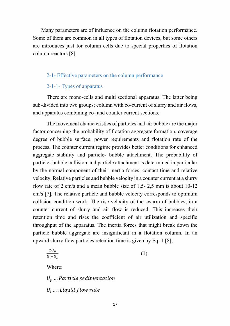
According to the Fig. 2-2, as operating bias is decreased, the carrying
capacity will increase. Decreasing the wash water rate or increasing the gas
rate can also decrease the bias rate [3]. The example of the latter is indicated
in Fig. 2-3. The results of the bias and gas rate were obtained from the
rougher column flotation on copper ore with 10 cm diameter of the column
cell. The data in fig. 2-3 was derived with two sparger fabrics, with fabric 2
being considerably more permeable than fabric 1 and thereby generating
larger gas bubble than fabric 1. The generation of larger gas bubbles can be
inferred from gas holdup measurement.
Fig. 2-2: Concentrate solid carrying rate versus bias rate [3]
20
Fig. 2-3: Effect of gas rate and bubble size on bias [3]
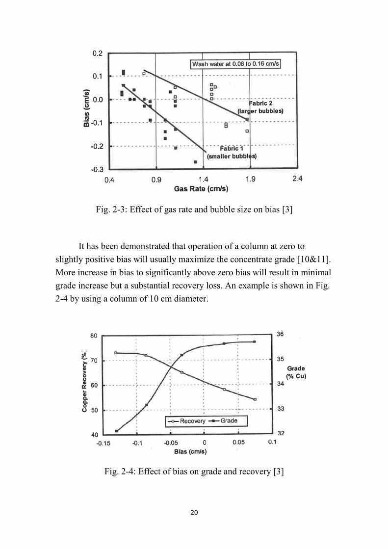
It has been demonstrated that operation of a column at zero to
slightly positive bias will usually maximize the concentrate grade [10&11].
More increase in bias to significantly above zero bias will result in minimal
grade increase but a substantial recovery loss. An example is shown in Fig.
2-4 by using a column of 10 cm diameter.
Fig. 2-4: Effect of bias on grade and recovery [3]

21
In some cases, it would be more profitable to run with a slightly
negative bias. A situation like this, arises when the column must process high
grade feed. If insufficient column capacity has been installed, it will be
difficult to operate the column with a positive bias while still attaining target
recovery.
The study, which has been carried out at Laval University
demonstrated the feasibility of an independent sensor for bias, which models
the relation between the conductivity profile across the interface and the bias
value using a neural network algorithm. A 250 cm height, 5.25 m diameter
plexiglas laboratory column was equipped with a series of conductivity
electrodes in its uppermost part (across the interface) to measure both, the
interface position and the bias rate. Using such equipment, the flotation
column dynamics was identified [12].
2-1-5- Gas Holdup
The gas holdup is the content of air inside the column. It is one of the
most important parameters since it characterizes the hydrodynamics of
bubbles in the co1umn cell [23, 24] and is a determining factor of the quantity
of bubble surface available for particle attachment. The gas holdup is a
function of a variety of variables in flotation and dependent to the bubble
size, which is a function of sparger type, frother properties, air flowrate,
compressed air pressure, machine and operational conditions, chemistry,
pulp flowrate, solid content and pattern of mixing in the collection zone. Gas
holdup is related to the flotation kinetics and defines the bubble surface area
flux. [13]
When gas is introduced into a column cell, liquid or slurry is displaced.
The volumetric fraction displaced is called the gas holdup (Ɛ𝑔) [13]. The gas
holdup is the fraction of gas in a gas-liquid or gas-pulp mixture. The
complement is the liquid or slurry holdup (1-Ɛ𝑔). The gas holdup is a
function of both gas rate and bubble size [3]. The magnitude of gas holdup
is a clue to the hydrodynamic condition of the collection zone.
22
The column feed port divides the column into two different zones. In
case that the lower zone contains 10% to 30% air, it is deemed to be
responsible for the bubble-particle attachment (i.e. for mineral recovery),
whereas the upper zone, which exhibits a 70 to 90% gas hold-up, is
responsible for the concentrate cleaning. This difference in gas hold-up
allows the detection of the interface between both zones, either by visual
observation in a transparent column or through any property related to the
air content, such as electrical conductivity, pressure or specific gravity [12].
The interface position, also called pulp level or froth depth, is another
important parameter of the column operation since it determines the relative
height of both zones. A taller bottom zone provides more residence time for
the bubbles to collect the mineral particles, thus increasing the recovery.
Consequently, this zone is called the collection zone or recovery zone [12].
The superficial velocity can be calculated by dividing the flowrate by
the column cross-sectional area. Hence, gas flowrate is often expressed as a
gas velocity 𝐽𝑔 (cm/s). The range of 𝐽𝑔 observed in industrial flotation
columns, at the top of the column, is typically between 1-2 cm/s [12].
𝐽𝑔 =𝑄𝑔
𝐴 (2)
Where:
𝐽𝑔 ..... Superficial gas rate (cm/s)
𝑄𝑔 .... Volumetric flow rate of gas (cm³/s)
𝐴 ...... Cross-sectional area (cm²)
2-1-6- Gas holdup measurement
The techniques for the measurement of gas holdup can be classified
into two categories: local and global measurements. Each of these methods
are described as follow.

23
a) Local Methods
Of the local measurement techniques, the most frequently used
methods are based on either electrical conductivity or X-ray absorption
which depends on the concentration of each phase [14]. In industry, because
of a lack of reliable method for on-line gas holdup measurement, it has been
considered as an unmeasured variable untill 2001. By this time a new
conductivity probe was developed to measure the electrical conductivity of
the slurry-gas dispersion [13].
Measurements have been performed in a 50 cm diameter and 4 m
length laboratory column flotation cell. In this column air is introduced by
eight vertical cloth spargers in a 40 cm ring through the column as shown in
fig. 2-5. The probe has been calibrated with some measurements which are
carried out by filling the cell completely with pure water. The actual gas
holdup values are determined during the experiments according to the
standard method, by means of pressure difference between two defined
points as will describe later. These series of experiments are carried out at
several air flowrates, using pure water, with and without surfactants [13].
Fig. 2-5:(1) Flotation Column, (2) Spargers, (3) Pressure Transmitters, (4)
Serial Communication Interface, (5) Computer, (6) Vertical Baffles, (7)
Mass flow Controller [13]

24
As a result of the measurements, the gas holdup value obtained from
conductivity is compered well with those from pressure difference in fig. 2-
6.
Fig. 2-6: Experimental result in two-phase water/air system [13].
The gas hold up value is also checked horizontally at different
positions. Following positions were chosen at the main vertical axis of the
column, midway between centre and body of the cell and the wall of the cell
via conductivity probe. The results illustrated that the gas holdup is
decreasing during its movement from vertical centre axis of the cell to the
cell body [13].
b) Global methods
There are two global methods, bed expansion and the manometric
technique based on pressure drop along the column. In a study, using the cell
shown schematically in fig. 2-7, global measurements were used. Each
measurement of gas holdup was repeated at least three times and the average
result is presented in all the following figures [14].
Fig. 2-7 shows the laboratory column set-up which is used for gas
holdup measurement. The column was constructed using a Plexiglas tube.
For most of the tests, water was the only feed and was fed through the wash
water inlet. Water flow rate was controlled by a variable speed pump
(Masterflex), and the discharge flowrate was controlled by a “Moyno” pump.

25
Compressed air was introduced into the column through a variety of spargers
whereas a flowmeter, calibrated at 20 psi, was used to regulate gas f1ow [14].
It was found that when no froth zone exists at the top of the column,
the two global methods are in good agreement. All experiments were
performed at room temperature.
Fig. 2-7: Laboratory Experimental Set-up [14]
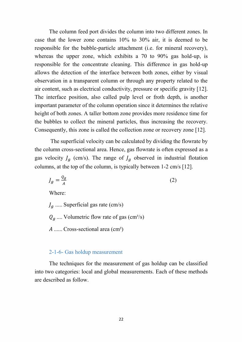
The relationship between Ɛ𝑔and 𝐽𝑔 is used to define the flow regime
[18]. Fig. 2-8 shows the general relationship between superficial gas velocity
and gas holdup. Gas holdup increases approximately linearly, then deviates
above a certain range of 𝐽𝑔 [15].
26
Fig. 2-8: Gas holdup as function of gas rate [16]
2-1-7- Bubble Generation
Bubble generation in column flotation cells is achieved via sparging
through pierced rubber or woven fabric such as USBM (US Bureau of
Mines) / Cominco and Minnovex. Some disadvantages of these sparger types
are:
Blockage
Tearing
Need to shut down to change
The large number required to maintain bubble size below 2-3 mm.
That approach is not common anymore, because of assessment or
replacement problems.
The second sparger types are those which are developed by the means
of jetting and shearing like MicrocelTM Column and the pneumatic cell
[14,15&17].
In jetting techniques, bubbles form as a result of instabilities on the jet
surface. Air is forced under high pressure (30-100 psig) and creates a jet of

27
air through the slurry. The bubble diameter is affected by the jet velocity.
This means a higher jet velocity produces smaller bubbles [16 & 17].
ρ𝐽𝑣𝐽 ...... jet momentum (per unit volume)
𝑛𝐵 ∝ 𝑙𝐽
𝑑𝐵 ∝1
𝑙𝐽
𝑙𝐽 ∝ ρ𝐽𝑣𝐽
𝑛𝐵 ........ the number of bubble
𝑑𝐵 ........ bubble size
lJ ........... jet length
As illustrated above, for producing a large population of fine particles,
a long jet length is required. Jet momentum can be increased by increasing
either the density or the velocity. In the USBM and Cominco design, ρ𝐽 is
increased by a small addition of water to the gas (normally ~ 1% of the gas
volume [14].
With the Minnovex, the approach is to control 𝑣𝐽 by adjusting the
annulus dimension and the gas pressure. A small annulus width (~1mm) and
gas pressure above ~45 psig together result in a velocity between 200- 400
m/s and produces at least a 50 cm long jet [17].
In Microcel™ column sparger, shear is achieved by the force slurry
and air over the blades of an in-line static mixer [18]. In the pneumatic cell,
feed slurry is forced through a constricted opening, reaching velocities of ~
4-6 m/s. with this setup, bubbles are produced by introducing air at a right
angle through a slot into the column. Due to the slurry velocity, the air is
sheared into fine bubbles.
28
2-1-8- Sparger Types
(a) Steel Sparger
The stainless steel sparger is available through the Flotation Column
Co. of Canada Limited. The number of orifices per unit area (porosity) is
quite low with respect to the dead area. The enlargement indicates, the holes
are not circular and there is a distribution of hole sizes. The average diameter
is approximately 50 µm. In addition, the orifices are distributed randomly
and the number of holes per unit area is difficult to estimate [14].
(b) Rubber Sparger
This type of sparger was recommended by Wheeler [19] and used at
Mines Gaspe. A photograph of the texture shows the regular distribution of
holes. The estimated porosity is around 42% and the average orifice diameter
is around 80 µm.
(c) Ceramic Sparger
The ceramic sparger was obtained from Fisher Scientific Inc. and is
often used in laboratory columns [86]. The average orifice diameter is 60
µm. The photography shows that the distribution of orifices is random and
porosity is higher in comparison with steel and rubber spargers. The texture
image indicates the shape of the orifices is not circular.
(d) Filter Cloth Sparger
Filter cloth sparger is a commonly used in "home-made" columns, due
to its low price and being easy to build. The structure is completely different
compared to the other types of sparger. It is not possible to estimate holes
size [14].

29
Fig. 2-9: Different types of spargers [14]
30
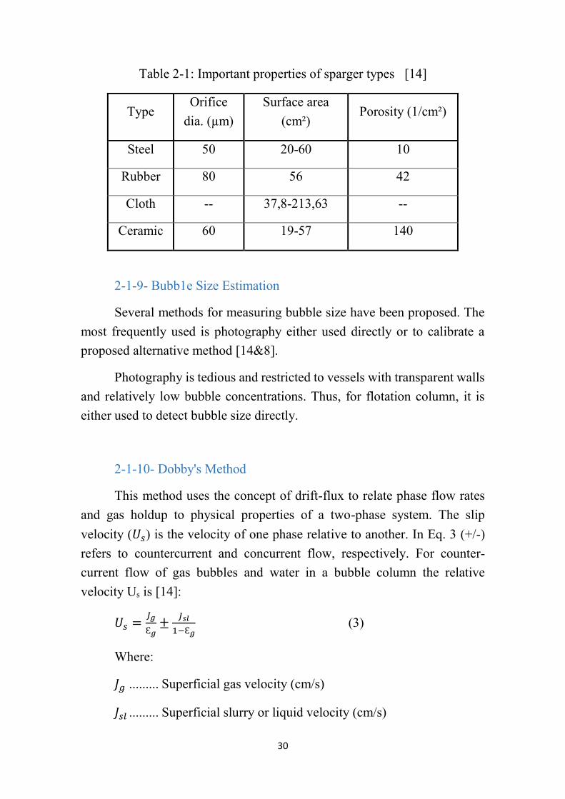
Table 2-1: Important properties of sparger types [14]
Type Orifice
dia. (µm)
Surface area
(cm²) Porosity (1/cm²)
Steel 50 20-60 10
Rubber 80 56 42
Cloth -- 37,8-213,63 --
Ceramic 60 19-57 140
2-1-9- Bubb1e Size Estimation
Several methods for measuring bubble size have been proposed. The
most frequently used is photography either used directly or to calibrate a
proposed alternative method [14&8].
Photography is tedious and restricted to vessels with transparent walls
and relatively low bubble concentrations. Thus, for flotation column, it is
either used to detect bubble size directly.
2-1-10- Dobby's Method
This method uses the concept of drift-flux to relate phase flow rates
and gas holdup to physical properties of a two-phase system. The slip
velocity (𝑈𝑠) is the velocity of one phase relative to another. In Eq. 3 (+/-)
refers to countercurrent and concurrent flow, respectively. For counter-
current flow of gas bubbles and water in a bubble column the relative
velocity Us is [14]:
𝑈𝑠 =𝐽𝑔
Ɛ𝑔±
𝐽𝑠𝑙
1−Ɛ𝑔 (3)
Where:
𝐽𝑔 ......... Superficial gas velocity (cm/s)
𝐽𝑠𝑙 ......... Superficial slurry or liquid velocity (cm/s)

31
Ɛ𝑔 ......... Fractional gas holdup (%)
A .......... Machine cross-sectional area (cm²)
The bubble surface area flux is derived as;
𝑆𝑏 = 6 ∗𝐽𝑔
𝑑𝑏⁄ (4)
Wallis [20] also postulated that Us is a function of terminal rise
velocity UT of a single bubble and the gas holdup, in the following form:
𝑈𝑠 = 𝑈𝑇(1 − Ɛ𝑔)𝑚−1 (5)
Where, “m” is a parameter defined according to Richardson and Zaki
[21] for 1<Re<200
𝑚 = [4,45 + 18𝑑𝑏
𝑑𝑐] ∗ 𝑅𝑒−0,1 (6)
And for 200<Re<500
𝑚 = 4,45 ∗ 𝑅𝑒−0,1 (7)
And the Reynold number is defined by:
𝑅𝑒 =𝑑𝑏𝑈𝑇𝜌𝐿
µ (8)
Where;
𝑈𝑇 ........ Terminal rise velocity of a single bubble (cm/s)
𝑈𝑇 is calculated by Eq. 3 and assuming Ɛ𝑔=0
Combining equation (3) & (5) gives:
𝑈𝑇 =𝐽𝑔
Ɛ𝑔(1−Ɛ𝑔)𝑚−1+
𝐽𝑠𝑙
(1−Ɛ𝑔)𝑚 (9)
Eq. (9) is derived assuming a uniform flow profile and uniform bubb1e
concentration across the co1umn cross-section, meaning:
a) Small superficial gas velocities (1-3 cm/s)

32
b) Normal distribution of bubble sizes, variance (± 20%)
c) Small average bubble size (0.5-2.0 mm)
d) No liquid circulation (this is reasonable for column diameters less
than 0.1 m)
For large columns, this is a reasonable assumption. For small columns,
correction factors are required and given by Bhaga [22].
Jameson [23] derived that the first order flotation rate constant (k) is
given by;
𝐾 = 1,5 ∗ 𝐸𝑐𝐽𝑔
𝑑𝑏 (10)
Where:
𝐸𝑐 ......... Collection efficiency, which is inversely proportional to the
square of the bubble size.
In addition, it has been found that the rate constant was not related to
the bubble size, gas hold up or superficial gas rate individually, but it was
related to bubble surface area flux. For instance, for shallow froth the
relationship was linear as;
𝐾 = 𝑃 ∗ 𝑆𝑏 (11)
Where:
P ........... Summarized the operational and chemical factors
Jameson showed that [23];
𝑃 =𝐸𝑐
4 (12)
2-1-11- Carrying Capacity
The rate of concentrate removal in terms of mass of solids overflowing
per unit time per unit column cross sectional area is generally referred to as
the carrying capacity of the column. This is related to the maximum

33
achievable coverage of air bubbles by particles and gives an upper limit to
the capacity of flotation columns. Moreover, the capacity of a flotation
column is limited by the amount of bubble surface available to carry the
particles into the froth launder [24]. The concentrate solid flux Ca (tph/m²),
in industrial columns, reches a value between 1-3 (tph/m²). This range
depends on the level of wash water and the concentrate particle size [3].
2-1-12- Estimation of Carrying Capacity
At a given superficial gas rate and bubble loading there is a certain
mass rate of solids that can be carried. A convenient unit is the mass of solid
carried per unit time per unit column cross-sectional area, or carrying rate
𝐶𝑟, given by [16];
𝐶𝑟 =𝜋𝐾1𝑑𝑝𝜌𝑝𝐽𝑔
𝑑𝑏 (13)
and,
𝐶𝑟,𝑚𝑎𝑥 = lim𝑑𝑏→0
𝐽𝑔→∞
𝜋𝐾1𝑑𝑝𝜌𝑝𝐽𝑔
𝑑𝑏 (14)
In general, the loaded bubbles will exhibit a larger 𝑑𝑝,𝑚𝑖𝑛 compared
to the unloaded bubbles. The increase is usually small and the effect will not
be pursued here [20].
Under normal column operating conditions, the quantity of solids
carried over into the froth through entrainment is low due to the effect of
wash water and can be neglected [24 & 25]. Furthermore, the size of particles
is also small compared to the size of the bubbles, except in cases such as coal
flotation. Under these conditions it can be shown that [26 & 27]
𝐶 = 𝐾. 𝐷𝑝𝜌𝑆𝑏 (15)
Where C is the carrying capacity (tph/m²),
K is an empirical factor which accounts for the particle packing on the
bubble surface
𝑑𝑝 ......... is a characteristic diameter of the particle in the froth (mm),

34
𝑆𝑏 ......... is the superficial bubble surface area rate (surface area of
bubbles passing through the column per unit time per unit cross
sectional area)
𝜌 ........... is the density of the particles in the froth (gr/cm³).
According to the equation (15), the carrying capacity for a given
product can be increased by increasing the superficial bubble surface area
rate, which in turn can be increased by increasing aeration rate or by reducing
the bubble size.
It was also concluded, that in the normal range of operation, air rate
and column diameter have only a marginal effect on carrying capacity [16,
28 & 29]
The maximum carrying capacity was related to the particle size and
density of solids in the froth according to the equation [30];
Cm = 0.068 dp ρ (16)
Where:
Cm ........ is the maximum carrying capacity (gr/min/cm)
dp ......... is the 80% passing size of solids in froth products (µm)
ρ .......... is the density of the particles in the froth (gr/cm³)
2-1-13- Column Height
The height of a column cell is determined by the required retention
time, accounting for both short circuiting and a significant degree of froth
dropback. In some cases, tall columns are undesirable. This arises when the
feed grade is high and the floatable minerals have high flotation kinetics.
This situation will cause the froth to become fully loaded and the retention
time is decreses [30].
Rubinstein [8] has shown in fig. 2-10, that when the solids content of
the feeds is relatively high (30%), the typical height of the collection zone
adversely affects the processing capacity of the column. The literature
suggests [31] that the phenomenon is due to the formation of aggregates with

35
high density, which may be entrained by the tailings discharge. According to
this, it is recommended to use high columns to float fine particles (10 µm),
and short columns for coarse particles (100 µm) [31]. Furthermore, Fig. 12
presents the results obtained by Maksimov et al., where is observed the
existence of an optimal hc/dc ratio that maximizes recovery [32]. Maksimov
et al. explains that when hc/dc > 5, the recovery may decrease as a
consequence of the loss of overloaded bubbles to the tailings [32].
An explanation similar to that is given by Kawatra et al [31]. In spite
of the apparent importance of these observations in column flotation, there
are few studies oriented to characterize this phenomenon and to identify the
experimental conditions that generate it.
Fig. 2-10: Effect of the ℎ𝑐
𝑑𝑐 ratio upon recovery [31]
2-1-14- Hydrodynamics of Flotation Machines
There are two main factors influencing the flotation process is depends
on; surface chemistry control and hydrodynamic conditions inside the
reactor cell.
The surface chemistry control leads to attachment of the bubbles to the
particle according to the potential conditions. Moreover, the hydrodynamic
conditions provide the attachment development and the movement of
particle- bubble to the froth [33].

36
2-1-15- Mixing Models
The particle collection process in a column is considered to follow
first-order kinetics relative to solid concentration with a rate constant. The
recovery of a first-order component process is dependent to rate constant,
mean residence time and mixing parameters [16].
a) Plug Flow:
One of the mixing models is plug flow transport. As it is illustrated in
fig 2-11, in this model, the residence time of all elements including fluid and
minerals is the same. Moreover, in the plug flow transport, the concentration
gradient of floatable mineral is along the axis of the column [16] and no
mixing occurred in the flow direction. This type of flow is mostly equivalent
to a batch processing system [34].
Fig. 2-11: Residence time distribution for plug flow and perfect mixing
[34]
𝑅 = 1 − 𝑒−𝑘𝑡 (17)
Where;
k ........... Constant rate
t ............ Retention time (min)

37
R .......... Recovery (%)
b) Perfect Mixing:
Another extreme mode is a perfectly mixed reactor, where a retention
time distribution exists and the concentration is the same throughout the
reactor.
In this flow model, the tracer is dispersed in the whole volume of the
device using a perfect mixing model and some of the tracer leaves the cell,
while some would never leave. Therefore, there is a distribution of residence
time from zero to infinity [34].
𝑅 = 1 −1
1+𝑘𝜏 (18)
Where;
𝜏 ........... Mean residence time (min)
In laboratory scale, using a typical laboratory flotation column
(diameter by 5 cm and 5 to 10 m high), the approaches show a plug flow
transport model, while in plant column is between plug flow and perfect
mixing flow.
Transport conditions that do not approach either of the two extremes
are usually described by one of two mixing models: tanks-in-series and plug
flow dispersion. A row of mechanical flotation machines is well suited to
tanks-in-series model and the flotation column. The plug flow dispersion
model provides a good description of an axial mixing process in the
collection zone.
Column dimensions can also be related directly to the plug flow
dispersion model parameters, but not to the tanks-in-series parameters. Thus,
a suitable model for the collection zone of a column, assuming a perfect
radial dispersion, is an axial plug flow dispersion model [16].
By impulse injection of a tracer at the top of the recovery zone and
measuring the concentrate of the tracer at a given distance below the

38
injection point, a function of turbulent mixing is obtained. The degree of
mixing is quantified by the axial dispersion coefficient (E). Furthermore, by
plotting the measured tracer concentration in the tailing stream against time
(starting from the injection time) a residence time distribution (RTD) is
achieved. The RTD can be modelled mathematically by using two
parameters to describe the mixing conditions; the mean residence time and
the vessel dispersion number [16].
𝑁𝑑 = 𝐸 (𝑢 ∗ 𝐻𝑐)⁄ (19)
Where;
u ........... Interstitial velocity (cm/s)
Hc ......... Height of collection zone (cm)
E .......... A direct function of cell diameter [(unit of length)²/time]
Nd ......... Vessel dispersion number (dimensionless)
𝐸 = 0,063𝑑𝑐 (𝐽𝑔
1,6)
0,3
2-1-16- Residence Time Distribution (RTD)
The efficiency is completely dependent on the time the material
spends in the machine of a flotation as a dynamic process. The residence
time distribution is the best indication of the flow pattern in the vessel.
The common way of RTD measurement is the injection of a tracer and
thus the detection of the concentration of this tracer in the outlet(s) against
time. The result of the distribution pattern is presented the ideal plug flow or
the ideal perfect mixing types which are shown in fig. 2-12 [34].
From the experimental data, mean residence time τ and variance Ϭ² of
the RTD are given by;
𝜏 =∑ 𝑡𝑗𝑐𝑗∆𝑡𝑗
∑ 𝑐𝑗∆𝑡𝑗 (20)
39
Ϭ² =∑(𝑡𝑗−𝜏)²𝑐𝑗∆𝑡𝑗
∑ 𝑐𝑗∆𝑡𝑗 (21)
∆𝑡𝑗 =(𝑡𝑗+1 − 𝑡𝑗−1)
2⁄ (22)
Where;
cj .......... Tracer concentration
tj ........... time (min)
Ϭ𝑟2 =
Ϭ²
𝜏² (23)
Ϭ𝑟2 ....... Relative variance
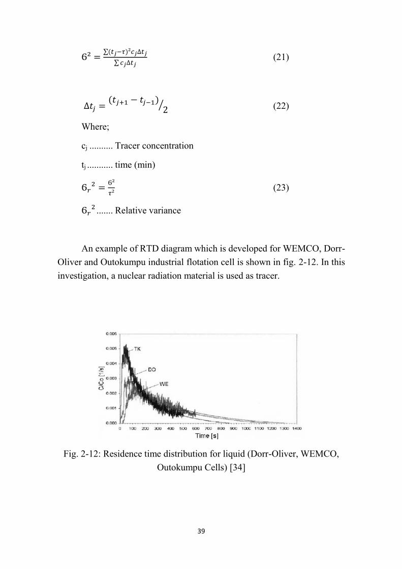
An example of RTD diagram which is developed for WEMCO, Dorr-
Oliver and Outokumpu industrial flotation cell is shown in fig. 2-12. In this
investigation, a nuclear radiation material is used as tracer.
Fig. 2-12: Residence time distribution for liquid (Dorr-Oliver, WEMCO,
Outokumpu Cells) [34]

40
When using the dispersion model, the feed and the discharge boundary
conditions should be known. Sampling from the tailing stream outside the
column satisfies the boundary conditions [16].
Ϭ𝑟2 = 2𝑁𝑑 − 2𝑁𝑑
2 [1 − 𝑒−1
𝑁𝑑] (24)
and
𝑢 =𝐻𝑐
𝜏 (25)
Bubble- particle collision probability models have been used to
analyse the height issues [35 & 36]. Defining the minimum height in order
to achieve at least one collision, the model shows that height is a strong
function of particle size. Heights can increase from less than 1m for > 50
(µm) particles to more than 10 m for <10 (µm) particles. An engineering
solution to the required height for a given process may develop from the
work of Ityokumbul [37]. He proposed to replace the common kinetic
approach with a mass transfer approach. This technique includes interaction
between the collection and froth zones as froth dropback can dominate
column design in some situations. To illustrate the need to consider these
interactions, one possible argument against tall columns is that the bubbles
become too loaded and this may reduce the solid carrying rate by overloading
the froth in a manner similar to that when a column is overfed [16]. The
decrease in recovery above a certain height observed by MAKSIMOV [32]
may have its origin in this effect. However, the overfeeding phenomenon has
never been explained. The capacity limitations, apparently imposed by the
froth, have led to testing “Zero Froth Column Flotation”.
2-2- Previous Case Studies
a) Generally, flotation in column cells has been simulated with models
based on the mixing characteristics prevailing in the cell [30]. For example,
Finch and Dobby [16] have proposed the axial dispersion model to describe
the mixing conditions of laboratory columns (2.5–10 cm of diameter) and
industrial columns (up to 2.5 m diameter). According to this model, the

41
knowledge of the mixing conditions helps to identify the relationship
between both grade and recovery and operational parameters such as
nominal residence time and relative flow rates of column streams. In this
theoretical approach, the height of the column, directly related to the
residence time, improves the mineral collection up to a point, where the
collection is limited by the carrying capacity (surface bubble saturation)
instead of being dictated by the flotation kinetics. The effect of the column
height on the flotation performance has been studied from an experimental
approach [36]. According to the authors, for a given capacity of the column
and constant feed flow rate, the recovery decreases and the grade increases
when the hc/dc ratio increases. Moreover, the authors suggest that it is
necessary to have a separation between the sparger and the tailing discharge,
to prevent the loss of the mineralized bubbles to the tailings stream.
b) In the investigation of a flotation column of an inside diameter of
15 cm and a total height of 8 m, all streams handling is achieved using
Masterflex peristaltic pumps. The pulp is prepared in a 250 lit capacity
conditioning tank, and is then transferred to another 250 lit tank, for
continues operation. The column feed port is located about 180 cm from the
column overflow lip. The concentrate overflows into a concentric launder
measuring 25 cm in diameter by 34 cm in tallest side height. The overflow
is also drained by gravity continuously [39].
Air is injected at the bottom of the column through a stainless steel
sparger, whereas wash water is sprayed over the overflowing froth via a
copper tube. Air and wash water flow rates are measured by an MKS mass
flow meter and a turbine flow meter. Feed, tailing and concentrate flow rates
are measured using magnetic flow meters.
Pulp- froth interface and bias rate are estimated from a conductivity
profile measured using eleven ring type stainless- steel electrodes mounted
flush against the inner wall of the column upper section. The various pairs
of electrode are sequentially excited to avoid current propagation between
the pairs [39].
c) The experimental program was conducted in a laboratory column
(0,057 m dia. & 4,5 m height), made of transparent acrylic tube. Actually,
42
the total column height was constant but the modification of the height of the
collection zone was easily accomplished, using a movable sparger (stainless
steel, 2 µm pore size). This sparger was suspended in the centre of the
column by a 3 mm OD vinyl air supply tube. The slurry is feed to the column
at 1.04 m from the overflow lip [30].
Others accessories of the column rig are a froth depth controller, a pH
meter (Omega 5T96), a conductivity meter (Orion model 162), a pulp
temperature controller and a photographic camera. This camera was installed
in front of the screen column section.
The mineral used to prepare the flotation pulp was silica sand with a
size distribution between 50 and 300 µm (d80 = 190 µm).
The experiments were performed in a closed circuit, with the aim to
keep the tailings flow rate (Jt) constant, wash water flow rate (Jww), gas flow
rate (Jg) and froth depth (hf ) at 1- 0,16- 1.46 cm/s and 0.3 m, respectively
[30].

43
Fig. 2-13: The laboratory column flotation [30]
d) The design of the semi-batch column is based on column flotation
practices and the concept of air lifting to keep solid particles suspended as in
Pachuca tanks [40]. The device, shown in Fig. 2-14, consists of an outer
column (measuring 75 cm tall * 7 cm dia.) and an inner column (measuring
15 cm tall * 3.8 cm dia.), both made of transparent plexiglass. Pulp
continuously flows up the inner column and down the annual space between
the two columns, thus providing the necessary retention time in a relatively
short column [40]. This manner of pulp circulation is achieved by injecting
compressed air into the inner column through a sparger which at the same
time provides the gas bubbles required for flotation.

44
A hemispherical baffle is installed at a distance of 2 cm above the inner
column for the purpose of preventing the slurry stream from directly
shooting up into the froth phase above. The baffle has 2.5 mm holes punched
onto its surface. Located at the top, typically 5 cm above the froth surface a
wash water sprayer in the form of a hollow ball is located. The semi-batch
column may be equipped with various auxiliary devices such as peristaltic
pumps, air flowmeter, solenoid valves, and pH meters [40].
Fig. 2-14: Schematic of the Semi-Batch Column [40]
The main operating variables of the semi-batch column include froth
thickness, pulp density, air flowrate and the amount of wash water. The froth
thickness was studied in the range of 5 cm to 30 cm, the pulp density in the
range of 10–35%, and the air flowrate in the range of 0.94–3.78 lit/min. The
column was operated with a pulp volume of 750 ml, and a flotation time of
3 min was applied in all tests. All three parameters were found to

45
significantly influence the flotation results, with the air flowrate having the
most impact. The froth wash water, which was applied at a rate of 440
ml/min in continuous mode and 1900 ml/min in intermittent mode, was
instrumental in obtaining cleaner froth products, as well as improving the
selectivity. It is recommended that for any given application, these variables
be carefully investigated and optimized [40].
e) The laboratory column cell was used for de-inking of waste paper
with 10 cm diameter and 470 cm length. The column was operated with
different sparger systems as porous stainless steel, filter cloth and jetting
spargers. The changed variables in the experiment were, the range of gas
rate, the retention time, froth depth and column height [41]. The gas rate was
accurately measured and controlled with a mass flow meter. Gas hold up was
measured by both pressure and conductivity method and the permitted
bubble size was estimated by drift flux analysis [42]. Data from the three
different sources are plotted together in Fig. 2-15. A linear relationship is
observed with a 95% relative confidence interval on the slope of ±3%.
Fig. 2-15: Bubble surface area flux and gas holdup in pilot and lab flotation
columns used for de-inking [42].

46
Chapter
Three:
Montan Column Flotation
Cell

47
3- Montan Column Flotation Cell
The cell has been designed and constructed according to several desire
demands and limitations of equipment.
A Free student version of AutoCad Inventor software is used to draw
a primary model of the cell with all details and dimensions. The cell is
including several parts to be accessible and easy to assemble and disassemble
such as; foam launder, the “Main Upper” part, middle main part, feed inlet,
conical bottom part, bubble generator, bubble generator holder and outlet
pipes for pressure measurement.
3-1- Foam launder
The foam launder, which has an inner diameter of 153,6 mm, is
constructed to collect the overflow foam at the top of the cell and is shown
in fig 3-1. The height of the launder is between 73,81 mm and 166,19 mm.
The bottom of the launder has a 30° incline. The details are referred in
appendix 1.
Fig. 3-1: Foam Launder
3-2- Main upper and middle parts
The main flotation chamber has an 81,4 mm inner diameter, of a 4,3
mm thickness, 300 mm height of the upper part and 1160 mm height of the
middle parts. The details are illustrated in appendix 2.
48
Fig. 3-2: Main upper and middle part
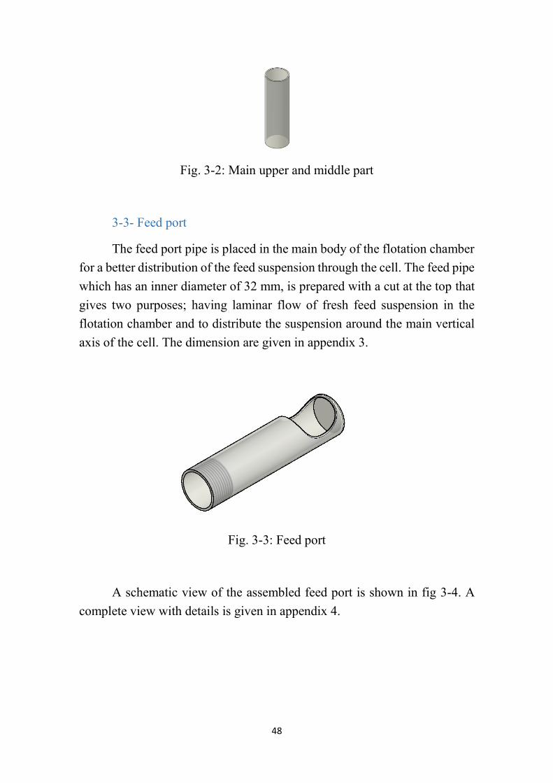
3-3- Feed port
The feed port pipe is placed in the main body of the flotation chamber
for a better distribution of the feed suspension through the cell. The feed pipe
which has an inner diameter of 32 mm, is prepared with a cut at the top that
gives two purposes; having laminar flow of fresh feed suspension in the
flotation chamber and to distribute the suspension around the main vertical
axis of the cell. The dimension are given in appendix 3.
Fig. 3-3: Feed port
A schematic view of the assembled feed port is shown in fig 3-4. A
complete view with details is given in appendix 4.

49
Fig. 3-4: A view of the assembled feed port on the main cell body
3-4- Conical bottom part
The designed conical shape part which is shown in fig 3-5 and
appendix 6, is placed at the bottom of the cell.
Fig. 3-5: Bottom conical part
3-5- Bubble generator
In order to disperse the bubbles through the cell, a porous tube bubble
generator is located in the cell near to the bottom. In principle, with injection
of compressed air through the bubble generator, the tube is expanded.
Therefore, the small holes are expanded in the texture of the tube and bubble
are released into the cell. The bubble generator, which produced by Eriez
company, is shown in fig. 3-6.

50
Fig. 3-6: Bubble generator
3-6- Bubble generator holder
One of the challenges during the design of the column was the
structure of the connections between the bubble generator, the cell body and
the compressed air pipe inside the cell. As bubble generator holder, a triple
pipe is used to keep the bubble generator synchronize with the main vertical
axis of the cell. The triple pipe, which is made of PVC-U polymer, is
connecting compressed air supply to the bubble generator. The holder is
shown in fig 3-7. This part is assembled near to the bottom of the cell. The
details are given in appendix 7.
Fig. 3-7: Bubble generator holder

51
Fig. 3-8: A schematic view of the bubble generator assembly
3-7- Outlet pipes for pressure measurement
There are two outlet pipes situated on the main cell body between the
feed port and the bubble generator holder to measure pressure difference.
This measurement is used for the gas holdup calculation. The outlet points
are shown in fig 3-9 and appendix 4.
Fig. 3-9: Outlet pipes for gas holdup measurement

52
3-8- Connections
Regarding to connect the mentioned parts of the cell, a screw
connector type is used. This type of connector is chosen, because it is easy
to assemble and disassemble. The details of the connector and dimensions
are given in appendix 9.
3-9- Cell assembly
In conclusion, the constructed column cell (fig. 3-10) has following
characteristics as shown in table 3-1:
Table 3-1: Montan column cell characteristics
Charactristic Value
Cell height 182 cm
Cell diameter 81,4 mm
Cell volume 9,5 lit
Distance between gas
holdup measurment outlets 80 cm
Maximum air pressure for
bubble generator 1 bar
Minimum air pressure for
bubble generator 0,25 bar

53
Fig 3-10: schematic view of final column designed
3-10- Conditioning tank
In order to prepare the feed slurry of the column, a barrel with 50 litre
capacity is used. Dry solid material, water and reagents are mixing in the
conditioning tank at desired solid content and a sequence of additives and
pH adjustment. Furthermore, a variable speed impeller is used to prepare the
pulp.
The amount of added water into the barrel is controlled by a water
flowmeter.
Fig. 3-11: Conditioning tank

54
3-11- Cell Control Procedure
To mix and prepare the feed suspension, a barrel with 50 lit capacity
and an electrical mixer are used as conditioning facilities. After mixing and
preparation of the feed pulp with desired reagents, the suspension is fed into
the cell to the desired level. At this time the discharge and air valves are
close. The desired level of suspension is adjusted until it reaches a level some
centimetres above the feed port to have enough depth of foam at the top of
the cell. Then, the discharge valve is opened to have a constant suspension
level in the cell. On the other hand, the income and outcome flowrates must
be equal. At this time, the air valve is opened to penetrate bubbles through
the column cell. As all used valves are controlled manually, the adjustment
of the operating condition such as input and output flowrates are difficult and
time consuming. To control the flotation column system, accurate alterations
of different parameters are important and have a large impact on the cell´s
performance.
A digital flowmeter is applied for feed flowrate determination. Based
on the digital flowmeter manual, the pipe at the location of flowmeter
installation must be full of suspension for a correct flowrate measurement.
For investigation reasons, it was necessary to run some experiments at lower
flowrates. In these cases, the digital flowmeter does not work properly. Thus,
the feed flowrate was adjusted at the desired flowrate by measurement of
suspension volume against time.
After each test, all containers and pipes must be cleaned to avoid
chocking.
As a summary, the instructions for the column cell are shown in fig
3-12 and the test implementation procedure is described step wise as
following:
1- The conditioning tank is filling with water for the feed flowrate
adjustment. At this time, all valves are closed except valves 1 and 2. As a
next step, valve number 2 is opened fully and the feed flowrate is set to the
desired flowrate by adjusting of valve 1. From now on, valve 1 will not
manipulated any more.

55
2- All valves, except valve 1, are closed to prepare the feed
suspension with a desired solid content in the conditioning tank.
3- Valve 3 is opened full to charge the column cell to the desired
level (usually some centimetres above the feed port). At this time, valve 5
is regulated as well to the desired wash water flowrate.
4- After achieving to the desired pulp level in the column cell, valve
7 is opened carefully to reach a constant level of suspension in the cell.
5- The air valve (valve 4) is opened to introduce air bubbles into the
flotation cell.
6- the system is cleaned after experiment with water.
Fig. 3-12: Schematic view of the column flotation cell and related facilities

56
Chapter
Four:
Experimented Material

57
Graphite and talcum ore have been chosen as testing material for the
constructed cell. The reason for selecting these types of material are
summarized below:
1- Having natural hydrophobicity property (easy to float)
2- Previous knowledge about the characteristic and mineralogy of
material
3- Enough amount of sample validity in the sample storage
4- Being easy to evaluate the products content via LOI and density
measurement.
5- Ban of chemical reagents usage
4-1- Graphite
4-1-1- A summary to graphite formation and structure
Graphite is a natural formation of crystalline carbon. As a mineral,
graphite forms when carbon is buried in the earth crust and in the upper
mantle under defined pressure and temperature. Graphite, which was
anciently referred to as Plumbago, is one of the allotropes of carbon,
semimetal and known as highest grade of coal. The phase diagram in fig. 4-
1 indicates the temperature and pressure condition of graphite formation.

58
Fig. 4-1: Graphite phase diagram [43]
Carbon forms a complex compound with hydrogen and other
minerals which are the basic of organic chemistry.
The structure of graphite consists of stacks of six-membered rings in
a sheet-like structure. Three neighbouring atoms are arranged at the apices
of equilateral triangles. In each carbon atom, three of four valance electrons
must be locked in tight covalent bonds with the three close neighbours. The
remaining electron is free to migrate across the surface of the sheet. This
structure provides the ability of graphite to be highly electrical conductive.
The graphite acts rather as a metal [43].
The distance between the sheets is slightly bigger than an atom
diameter and is calculated at 0,34 nm. The Van der Waals bonding between
the stacks is very weak and perpendicular to them. Having such an open
structure implies that the occupied space of the total available space is only
20 %, thus accounting for the relatively low density of graphite.
Physical features of graphite [43]:

59
Apart from the perfect diagnostic basal cleavage, other
cleavage planes have been identified.
The hardness property of graphite lies between 1 and 2
according to Mohs´ scale
Graphite has mark paper and soil fingers properties
The density is between 2,09 gr/cm³ and 2,23 gr/cm³ (lighter
than its paramorphism diamond at 3,52 gr/cm³.
The color is varying from shining black to dull.
Graphite has high electrical conductivity property parallel to
the sheets and semi-conductivity property perpendicular to the
atomic carbon sheets
Graphite is transparent to X-rays.
The main difference between graphite and diamond is that the carbon
bonding involves sp³ hybridization in diamond and sp² hybridization in
graphite. As a result, diamond has three-dimensional crystal structure,
whereas graphite consists of carbon layers with covalent and metallic
bonding within layers. The electrical conductivity property of graphite leads
to use as electro-chemical electrodes. As a result of this anisotropy, the
carbon layers can slide with respect to one another quite easily, thus making
graphite a good lubricant and pencil material.
Graphite generally occurs as a result of metamorphism of organic
matter in sediments. As metamorphic grade increases, carbonaceous material
converts to amorphous graphite [44]. Vein graphite is assumed to form by
partial volatilization of graphite and subsequent recrystallization during
regional granulite and / or charnockite faces metamorphism. Amorphous
graphite is generally considered to have originated by thermal or regional
metamorphism of coal or carbonaceous sediments [43].
Impurities include minerals as for instance, quartz, mica, calcite,
feldspar, amphibole, garnet, with occasional amphiboles, pyrrhotite,
magnetite and magnetite.
Graphite is used mainly for lubricants, pencils, batteries, brake lining,
conductive coatings, bearing, refractories and crucibles.

60
4-1-2- Processing of Graphite
According to the mentioned graphite structure, gangue minerals and
property descriptions, density separation, electrostatic separation and
flotation can be variable options of beneficiation wit regard to mineral
processing. Other conditions such as intergrowth and particle size
distribution must be considered for processing method selection as well.
Graphite can easily be enriched by flotation because of its high natural
hydrophobicity properties, especially in the small particle size range. As
collector, kerosene, paraffin, diesel oil, fuel oil or ionic collectors like
potassium amyl xanthate, dithiophosphate are commonly used. As frother,
pine oil or MIBC (Methyl isobutyl carbinol are used. Sodium silicate,
quebracho and starch are used to depress gangue minerals [43].
4-2- Talc
Talc is a widely used industrial mineral, which is composed of hydrated
magnesium sheet-silicates with a theoretical formula of
Mg3Si4O10(OH)2 that belongs to the phyllosilicate family [45]. Talc
applications including ceramics, cosmetics, pharmaceuticals, paints, plastic,
paper, roofing felt, insecticides, rubber and others. For each case of talc
application, various degrees of purity are required. For instance, low grade
talc is used as a filler in drywall sealing compounds, medium grade finds its
application in paper industry and high grade is mainly required in cosmetic
and pharmaceuticals. Most applications need fine grained talc and a
minimum of asbestiform particles [46].
Talc consists of a two dimensional sheet structure forming two layers of
silica tetrahedral held together with octahedral brucite [47]. Talc surface is
comprised of two types of surface area, the basal cleavage faces and the
edges. It is believed that the talc faces are non-polar and hydrophobic
because, the faces surface has no charged group, whereas the edges are
hydrophilic due to the presence of charged ions (Mg2+ and OH−). The major
gangue minerals of talc are carbonates, magnesite, dolomite, serpentine,
chlorite and calcite, which contribute to undesirable characteristics. The
trace minerals include magnetite, pyrite, quartz and tremolite. The

61
percentage of some constituents in talc such as calcium oxide, iron oxide and
aluminium oxide determine the quality of talc samples for market demands
[48].

62
Chapter
Five:
Column Cell Flotation
Experiments & Results

63
The performance of the constructed cell was evaluated by flotation
experiments with the talc and graphite ore. Moreover, some of the operation
parameters were measured during these experiments such as the bias rate and
the gas holdup. The procedure of the tests and the evaluation methods are
described as following.
5-1- Material evaluation
To characterize the flotation products competitively, simple and quick,
the density and LOI measurements were used.
5-1-1- Density measurement
During all the experiments, the solid density has been measured by
helium pycnometer which is provided by micromeritics company model
AccuPyc 1330. The helium pycnometer measures the volume of sample in
the sample cup. The measurement principle is based on the ideal gas equation
(equation 26) using the measurement of pressure to determine the volume of
a sample.
𝑃𝑉 = 𝑛𝑅𝑇 (26)
Where;
n ........... number of mole of gas (mole)
R .......... universal gas constant (R= 8,314 𝐽
𝐾.𝑚𝑜𝑙)
V .......... volume (cubic metres)
P ........... gas pressure (pascal)
T .......... temperature (Kelvin)

64
5-1-2- Loss of ignition (LOI)
The LOI test was used for both the graphite and talc ore samples for
products evaluation, but under different conditions. In both cases, the usual
and standard procedures were used for each type of sample.
a) LOI test of graphite ore
Has been carried out with around one gram of dry sample in the
ceramic sample cup. The experiment was performed on the graphite ore
material as received. The particle size of sample was determined at 100% -
100 µm. At first, the sample was heated up to 425 degree Celsius in the
furnace for two hours. At this temperature, the sample release the moisture.
Preheating of the sample leads to measurement of the carbon content more
accurate. The stepwise procedure of the LOI test for graphite ore is explained
as follow:
Measurement of sample mass in the cup.
Preheating to 425 degree Celsius for two hours.
Sample mass measurement
Heating at 1025 degree Celsius to oxidize carbon content for 8
hours
Mass measurement of burnt sample.
b) LOI test for Talc
The used sample mass, as same as graphite, is around one gram in the
ceramic sample cup. The sample was heated up at 1050 degree of Celsius for
one hour.
5-1-3- Determination of carbon and sulphur content
LECO Company is the supplier of the apparatus for carbon and
sulphur content measurement. Therefore, this method of carbon and sulphur
analysing is known as “LECO” method. This experiment was carried out
only on the products of the column flotation test with talc ore. In principle,

65
the sample is combusted at high temperature so that all the carbon and
sulphur contained oxidized to CO2 and SO2 form, respectively. The device
is equipped with an infrared detector to record the concentration of CO2 and
SO2 [49].
5-2- Talc sample characteristics and preparation
The talc ore sample originates from Gemersha Polowa mine, which is
located in Slowakia. In table 5-1, the particle size distribution, LOI and
density values of each fraction, according to the described procedures in
section 5-1-1 & 5-1-2, are illustrated. As sample preparation for LOI and
density measurements on coarse fractions (+200 µm), the sample was ground
by mortar and pistil to achieve a suitable particle size for measurements.
Table 5-1: Result of manual screen analysis as well as LOI and density
measurements in size classes
Fraction
(µm) Mass (gr) Mass (%)
Cum.
Passing
(%)
LOI (%) Density
(gr/cm³)
+8000 132,7 3,3 96,7 14,30 2,86
+6300-8000 356,2 8,9 87,7 15,12 2,83
+4000-6300 683,8 17,1 70,6 15,06 2,86
+3150-4000 276,0 6,9 63,7 14,91 2,85
+2000-3150 490,6 12,3 51,4 15,94 2,86
+1250-2000 414,4 10,4 41,0 16,21 2,89
+710-1250 417,4 10,5 30,5 15,41 2,88
+500-710 218,0 5,5 25,1 15,41 2,89
+315-500 245,0 6,1 18,9 15,40 2,88
+250-315 110,2 2,8 16,2 15,08 2,89
+125-250 248,4 6,2 9,9 14,34 2,89
-125 396,6 9,9 0,0 10,87 2,87
SUM 3989,33 100 Ave. 14,87 2,87

66
Based on the microscopic investigations on the talc ore in the particle
size range of -63+40 µm, quartz and dolomite are encountered as the main
gangue minerals apart from pyrite. For the nominal (modal) composition, all
the carbonates are calculated as dolomite. From the known carbon and
sulphur content of the dolomite [(CaO)(MgO)(CO2)2] and pyrite [FeS2] and
the measured carbon and sulphur content in the sample, the total content
of dolomite and pyrite were estimated. The nominal loss of ignition of
pure talc is given by 4,75% [48].
From the decomposition reaction of dolomite, which is;
(CaO)(MgO)(CO2)2→(CaO)(MgO)+2CO2↑
and pyrite oxidation reaction, which is
FeS2+11O2→Fe2O3+4SO2↑
The relative weight loss of dolomite related to carbon content (4,02
gr/gr of carbon) and the relative weight loss of pyrite related to the sulphur
content (0,626 gr/ gr of sulphur) were calculated. Thus the nominal mineral
system was resolved from LOI and density measurement as well as the
carbon and sulphur contents in the following way. The mineralogical
composition within the size classes was determined by a combination of
physical and chemical analysis. The physical analysis included
Manual sieve analysis of a sample
Fraction +10 mm was subdivided into density classes by sink-
float analysis.
Particle density measurement
LOI measurement
The density of pure minerals were determined by the helium
pycnometer on manually collected samples of pure minerals (mineral
standards). The results are given in table 5-2.

67
Table 5-2: Density of pure minerals [50]
Mineral Density
Pyrite 5,20 gr/cm³
Dolomite 2,963 gr/cm³
Talc 2,792 gr/cm³
The LOI value of the minerals were determined on ground samples in
the furnace by heating at 1050 degree of Celsius for one hour.
The analysis results of carbon and sulphur content, by combustion at
high temperature followed by infrared detection of CO2 and SO2 on the
dolomite and talc standard are given in table 5-3.
Table 5-3: Carbon and sulphur content analysis of dolomite and talc
standard [50]
Carbon
content (%)
Sulphur
Content (%)
Dolomite 12,7 0,05
Talc 0,29 0,01
The particle of fraction +10 mm were measured for particle density,
subdivided into density classes and prepared for carbon and sulphur analysis
by comminution.
The size classes +2-4 mm, +1-2 mm, +0,5-1 mm, +0,315-0,5 mm,
+0,2-0,315 mm were analysed by sink-float analysis at 3,12 gr/cm³ liquid
density [50].
The applied equations in table 5-4 are as follow:
Dolomite Content= Carbon Content/0,1302 (27)
Pyrite Content= Sulphur Content/0,5306 (28)
LOI Calculated = 4,02*(Carbon content)+ 0,626*(Sulphur content)
(29)

68
LOI residue=LOI measured – LOI calculated (30)
Talc content= (LOI residue)/0,0475 (31)
Residue Mineral Content= 100- Talc content- Dolomite content- Pyrite
content
Table 5-4: Mineralogical investigation of talc sample [50]
Talc (%)Dolomite (%)
Pyrit (%)Rest M
inerals (%)
2,39-2,654,32
2,725,91
0,5600,750
2,723,19
674
127
2,65-2,704,94
2,661,11
0,1600,060
0,680,43
91
090
2,71-2,758,02
2,764,91
0,5000,004
2,012,90
614
035
2,76-2,8030,25
2,767,9
1,2400,080
5,032,87
6010
030
2,81-2,8529,01
2,807,83
0,8900,600
3,953,88
827
110
2,86-3,2523,46
2,8512,68
2,5802,460
11,900,78
1620
559
+4-1023,38
2,817,09
0,8750,477
3,813,28
697
123
+2-412,05
2,798,87
1,1700,098
4,764,11
879
04
+1-212,05
2,798,35
1,1400,056
4,613,74
799
012
+0,5-14,22
2,818,46
1,1800,049
4,773,69
789
013
+0,315-0,53,23
2,798,52
1,1800,027
4,763,76
799
012
+0,2-0,3153,33
2,798,26
1,0700,016
4,313,95
838
09
-0,2 12,47
7,10,670
0,1302,77
4,3391
50
3
Calculated
LOI (%)
Meas. LOI -
Cal. LOI (%)
Mineral Composition
+10
Size Classes
(mm)
Density Classes
(gr/cm³)
Mass
(%)
Density
(gr/cm³)LOI (%)
Carbon
Content (%)
Sulphur
Content (%)
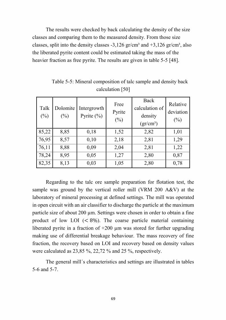
69
The results were checked by back calculating the density of the size
classes and comparing them to the measured density. From those size
classes, split into the density classes -3,126 gr/cm³ and +3,126 gr/cm³, also
the liberated pyrite content could be estimated taking the mass of the
heavier fraction as free pyrite. The results are given in table 5-5 [48].
Table 5-5: Mineral composition of talc sample and density back
calculation [50]
Talk
(%)
Dolomite
(%)
Intergrowth
Pyrite (%)
Free
Pyrite
(%)
Back
calculation of
density
(gr/cm³)
Relative
deviation
(%)
85,22 8,85 0,18 1,52 2,82 1,01
76,95 8,57 0,10 2,18 2,81 1,29
76,11 8,88 0,09 2,04 2,81 1,22
78,24 8,95 0,05 1,27 2,80 0,87
82,35 8,13 0,03 1,05 2,80 0,78
Regarding to the talc ore sample preparation for flotation test, the
sample was ground by the vertical roller mill (VRM 200 A&V) at the
laboratory of mineral processing at defined settings. The mill was operated
in open circuit with an air classifier to discharge the particle at the maximum
particle size of about 200 µm. Settings were chosen in order to obtain a fine
product of low LOI (< 8%). The coarse particle material containing
liberated pyrite in a fraction of +200 µm was stored for further upgrading
making use of differential breakage behaviour. The mass recovery of fine
fraction, the recovery based on LOI and recovery based on density values
were calculated as 23,85 %, 22,72 % and 25 %, respectively.
The general mill´s characteristics and settings are illustrated in tables
5-6 and 5-7.

70
Table 5-6: VRM 200 Characteristics
Mill type Vertical roller mill
Maximum throughput 100 kg/hour
Diameter of plate 200 mm
Nominal power draw of motor to rotate the plate 5 KW
Number of rollers 2
Roller diameter 13 cm
Nominal ventilation power 18 KW
Classifier´s cage diameter 15 cm
Maximum rotational speed of cage 4000 rpm
Cut size with nominal air volume (1000 m³/h) 50 µm
Table 5-7: Mill settings for talc sample grinding
Feed flowrate 20 kg/h
Plate rotational speed 65 rpm
Roller downward pressure 15 bar
Distance between rollers and plate 3 mm
Roller upward pressure 11 bar
Ventilator rotational speed 1500 rpm
Classifier´s cage speed 1500 rpm
Table 5-8 shows the data obtained from four series of sampling during
comminution. The samples were taken from coarse and fine streams of the
air classifier for a duration of 220 sec. The reason for selection of 220 sec as
the sampling duration was the air classifier filter. The filter of the air
classifier contains four filter batteries and every 55 seconds, the battery
changes for discharge. To obtain a representative sample, the samples were
taken from a complete filter cleaning circuit.
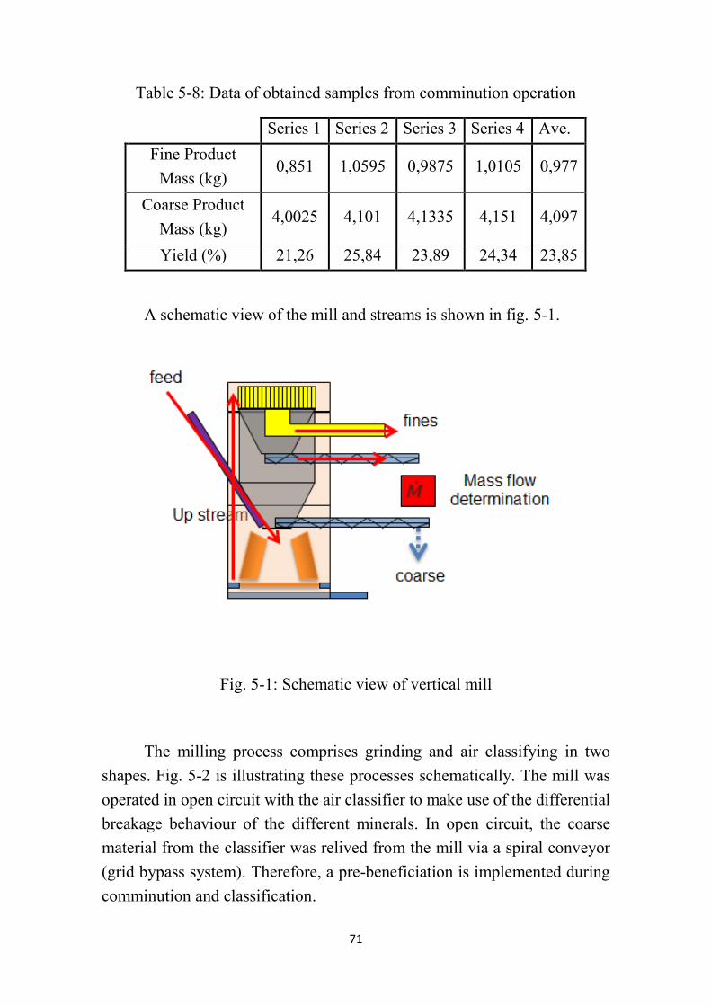
71
Table 5-8: Data of obtained samples from comminution operation
Series 1 Series 2 Series 3 Series 4 Ave.
Fine Product
Mass (kg) 0,851 1,0595 0,9875 1,0105 0,977
Coarse Product
Mass (kg) 4,0025 4,101 4,1335 4,151 4,097
Yield (%) 21,26 25,84 23,89 24,34 23,85
A schematic view of the mill and streams is shown in fig. 5-1.
Fig. 5-1: Schematic view of vertical mill
The milling process comprises grinding and air classifying in two
shapes. Fig. 5-2 is illustrating these processes schematically. The mill was
operated in open circuit with the air classifier to make use of the differential
breakage behaviour of the different minerals. In open circuit, the coarse
material from the classifier was relived from the mill via a spiral conveyor
(grid bypass system). Therefore, a pre-beneficiation is implemented during
comminution and classification.

72
Fig. 5-2: Sequence of processes in the vertical roller mill
Tables 5-9 and 5-10 show the particle size distribution (PSD) of coarse
and fine fractions of the mill, respectively. The size distribution diagram is
also illustrated in fig. 5-3.
Table 5-9: VRM200. Result of screen analysis of the coarse fraction of the
mill product
Size(µm) Mass (gr) Mass (%) Cum. Passing
(%)
+1000 2,96 1,29 98,71
+500-1000 55,8 24,37 74,33
+250-500 68,03 29,72 44,62
+100-250 60,37 26,37 18,25
+60-100 27,22 11,89 6,36
+50-60 5,75 2,51 3,84
+25-50 6,85 2,99 0,85
-25 1,95 0,85 0,00
SUM 228,93 100
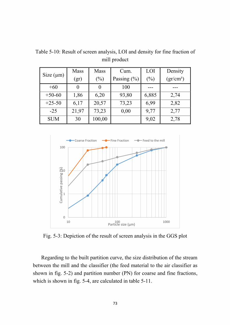
73
Table 5-10: Result of screen analysis, LOI and density for fine fraction of
mill product
Size (µm) Mass
(gr)
Mass
(%)
Cum.
Passing (%)
LOI
(%)
Density
(gr/cm³)
+60 0 0 100 --- ---
+50-60 1,86 6,20 93,80 6,885 2,74
+25-50 6,17 20,57 73,23 6,99 2,82
-25 21,97 73,23 0,00 9,77 2,77
SUM 30 100,00 9,02 2,78
Fig. 5-3: Depiction of the result of screen analysis in the GGS plot
Regarding to the built partition curve, the size distribution of the stream
between the mill and the classifier (the feed material to the air classifier as
shown in fig. 5-2) and partition number (PN) for coarse and fine fractions,
which is shown in fig. 5-4, are calculated in table 5-11.
0
1
10
100
10 100 1000
Cu
mu
lati
ve p
assi
ng
(%)
Particle size (µm)
Coarse Fraction Fine Fraction Feed to the mill

74
Table 5-11: Calculated partition numbers for coarse and fine products of
vertical roller mill
Size (µm) Mass (%) Coarse PN
(%)
Fine PN
(%)
+1000 0,98 100 0
+500-1000 18,56 100 0
+250-500 22,63 100 0
+100-250 20,08 100 0
+60-100 9,05 100 0
+50-60 3,39 56,40 43,60
+25-50 7,18 31,72 68,28
-25 18,11 3,58 96,42
Fig. 5-4: VRM200. Partition curve of coarse material according to the
setting of the mill and classifier given in tables 5-6 and 5-7
0
10
20
30
40
50
60
70
80
90
100
0 10 20 30 40 50 60 70 80
Par
titi
on
Nu
mb
er (
%)
Particle Size (µm)
Coarse Partition Curve

75
The partition curve values are also calculated from fig. 5-4 as shown
in table 5-12.
Table 5-12: Characteristics figures derived from the partition curve fig. 5-4
T 50 T 75 T 25 Cut Size ep Imperfection
Values 53
µm
58
µm
32
µm 53 µm
13
µm 0,24
𝑒𝑝 = 𝑇75−𝑇25
2 (32)
Imperfection =𝑇75−𝑇25
2𝑇50 (33)
T50 ....................... Tromp value
T75 ....................... particle size at 75% of partition number
T25 ....................... particle size at 75% of partition number
ep .......................... Écart probable
Imperfection ......... the Écart probable related to the Tromp value
5-3- Bias measurement
Regarding to the wash water flowrate determination, an experiment
was implemented to measure the bias rate against the wash water flowrate
alteration. As it is discussed before, a zero or even slightly positive bias rate
gives the best results regarding the concentrate grade and recovery. In
contrast, the wash water flowrate must be big enough to penetrate into the
cleaning zone.
The experiment was performed continuously in presence of the frother
without solids. The flowrate of the overflow stream was measured with and
without wash water stream.
The rate of overflow stream was measured at 0,5 cm³/sec without wash
water stream. Then, the experiment, at the same operation conditions, was

76
repeated in the presence of the wash water stream at 5,5 cm³/sec flowrate.
The latter rate of overflow stream was obtained 2 cm³/sec. The summarized
information of the measurement is shown in table 5-13.
Table 5-13: Results of bias measurement
Parameter Value Dimension
Feed flowrate 0,7 lit/min
Wash water flowrate 0,33 lit/min
Discharge flowrate 1,03 lit/min
Overflow rate without wash
water 0,03 lit/min
Overflow rate with wash
water 0,12 lit/min
Foam height 26,5 cm
Differential pressure 12,5 cm
Gas holdup 15.6 %
Compressed air pressure 0,3 bar
Bias rate 0,02 cm/sec
The bias rate in table 5-13 was calculated as follow:
Cell cross section area: 𝐴𝐶 = 52,04 cm²
Overflow rate difference with and without water: 𝑄𝑤 = 1,5 cm³/sec
According to the superficial velocity formula, as mentioned in chapter
two:
𝐽𝑤 =𝑄𝑤
𝐴𝑐= 0,02 𝑐𝑚/𝑠𝑒𝑐 (34)
From now on, in the all flotation column experiments, the wash water
flowrate is set at 0,33 lit/min up.

77
5-4- Flotation column test on talc ore
The test was carried out with the talc ore, the fine fraction product of
the VRM200 with mentioned properties under the desired operation
conditions as shown in table 5-14.
Table 5-14: Talc Column Flotation Operation Condition
Preparation of Suspension
Conditioning
Tank Vol.
Vol.
Solid
Content
Solid
Density
Solid Mass
of
Water
Pulp
Density
Retention
Time Vol. Mass
50 lit 4% 2,83
t/m³
0,002
m³
5,66
kg 48 kg
1,073
t/m³ 210 sec
The column flotation experiments are aimed at a better understanding
of the flotation cell behaviour and parameters. Therefore, some parameters
like solid content of suspension and reagents dosage are not optimized. The
adjusted values were obtained from literature and used only to proof the cell
performance. After preparation of the feed pulp in the conditioning tank, the
natural pH value of the slurry was measured at 8,25. The retention time was
also controlled by adjustment of the feed flowrate according to the cell
volume (9,5 lit). During this experiment, the feed and the wash water
flowrates were manipulated at 2,7 lit/min and 0,33 lit/min, respectively. In
order to keep the pulp level constant in the flotation cell, after filling up the
cell till the desired level (about 10 centimetres above the feed port), the
discharge flowrate was set up at 3,03 lit/min manually.
At this time the air valve was opened to inject the compressed air
through the bubble generator at 0,3 bar pressure.
The only used additive as reagent, was frother (70 gram of MIBC per
ton of dry solid). Therefore, the mass of the used frother according to the dry
solid mass was calculated 0,4 gr.

78
Several series of samples from the foam and the discharge streams
were taken during the experiment running time. In this experiment, each
sample was taken for 10 sec. Because of being single operator, sampling was
not performed, simultaneously. In each series of sampling, a complete cross
section of the foam and the underflow streams was sampled. For the second
and the third series of sampling, the mentioned sequence was repeated. From
the obtained results by sampling, the mass balance table is formed in table
5-18. Table 5-15 shows the time schedule of the activities.
Table 5-15: Time schedule of talc ore experiment activities
Time schedule
Mixer was started at 0 min
Reagent was added at 5 min
Feed valve was opened at 17 min
Air valve was opened at 26 min
Sampling 1 at 31 min
Sampling 2 at 36 min
Sampling 3 at 43 min
During this experiment, the compressed air pressure was adjusted at
0,3 bar and the differential pressure on gas holdup hoses was read at 9 cm.
Therefore, the gas holdup, according to the equation 27, was calculated 11,2
%.
Gas Holdup (%) = 𝛥ℎ
𝐻∗ 100 (35)
Where:
“𝚫h” is the difference level of pulp or liquid in gas holdup hoses and
“H” is referred to the distance between to gas holdup outlets on the column
cell body,

79
Table 5-16: Summarized features of talc ore column experiment
Parameter Value Unit
Difference height in gas holdup hose 9 cm
Gas holdup 11,2 %
Collection zone height 150 cm
Cleaning zone height 31,8 cm
The details of obtained samples are shown in table 5-17.
Table 5-17: Samplings data
Sample Name
Mass of
Suspension
(gr)
Mass of
Dry solid
(gr)
Sam. 1 Conc 205,67 23,59
Sam. 1 Tail 135,07 8,99
Sam. 2 Conc 142,05 19,28
Sam. 2 Tail 530,32 25,36
Sam. 3 Conc 355,95 38,92
Sam. 3 Tail 1070,68 74,44
Each single sample was washed at 25 (µm) to determine the flotation
behaviour on the fine particles. Therefore, each sample was divided into two
fractions, +25 µm and -25 µm. Afterwards, the samples were dried at 60

80
degree Celsius to avoid pyrite mineral oxidation. The mass balance table,
which is shown in table 5-18, was developed according to the dry mass of
samples, LOI and density values. The LOI and density values were gained
as it described in section 5-1-1 & 5-1-2.
Table 5-18: Mass balance table for talc column flotation experiment
Sam
pleM
ass
(gr)
Mass
recovery
(%)
Fraction
(µm
)
Mass
(gr)
Yield in
sampling
series
(%)
Mass
Recovery
of Coarse
(%)
Mass
Recovery
of Fine
(%)
Density
(gr/cm³)
Density
in
product
(gr/cm³)
LO
I (%)
Size
related
LO
I
recovery
(%)
LO
I in
product
(%)
LO
I recovery
(%)
(100-LO
I)
recovery
(%)
+25
9,0527,78
78,962,85
5,3366,48
-2514,54
44,6368,85
2,886,45
53,45
+25
2,417,40
21,042,87
10,1033,52
-256,58
20,1931,15
2,8412,42
46,55
+25
11,46100,00
2,856,34
100,00
-2521,12
100,002,86
8,31100,00
+25
8,3218,64
64,172,86
5,2445,11
-2510,96
24,5534,61
2,846,30
20,37
+25
4,6510,41
35,832,81
11,4154,89
-2520,71
46,4065,39
2,8013,02
79,63
+25
12,97100,00
2,847,45
100,00
-2531,67
100,002,82
10,69100,00
+25
19,7017,38
49,002,83
5,2440,43
-2519,22
16,9521,77
2,846,79
15,71
+25
15,7713,91
51,002,80
9,6559,57
-2558,67
51,7678,23
2,8111,94
84,29
+25
35,47100,00
2,827,20
100,00
-2577,89
100,002,82
10,67100,00
93,99
88,55
90,42
35,69
64,31
100,00
5,84
12,73
6,01
11,45
73,66
26,34
100,00100
100
2,85
2,80
2,829,75
94,16
87,27
90,25
45,07
54,94
100,00
2,8693,98
88,21
92,39
72,416,02
Feed S
3113,36
Conc. S
1
Tail. S
1
Conc. S
2
Tail. S
2
Conc. S
3
Tail. S
3
23,59
8,99
19,28
25,36
38,92
74,44
Feed S
132,58
Feed S
244,64
27,59
43,18996
56,81004
34,33
65,67
2,85
2,86
2,84
2,81
1002,82
9,58
11,79
7,61

81
The average recovery of LOI during the talc ore flotation column
experiment was gained at 44,37%. As it is shown in table 5-18, the LOI
values for concentrate and feed (table 5-18) are not constant. Therefore, the
related recoveries are also different.
One of the reasons of the mentioned inconstancy in table 5-18 might
be the instability in column cell operation conditions. Stable conditions in
semi-batch processing systems as well as continuous systems, need time to
establish. In other words, process stability is time dependent. In order to have
more time to achieve stability in the lab column flotation process
implementation of increased capacity of the conditioning tank is necessary.
In addition, operation conditions such as feed flowrate and
compressed air flowrate during flotation experiments must be kept constant
to reach stabilization. Alterations of slurry level in the conditioning tank,
unsuitable shape and dimensions of impeller cause of changes in feed slurry
flowrate. In order to keep the feed flowrate and underflow rate constant, it is
necessary to use pumps of adjustable flowrate for both streams.
Because of absence of pumps, the conditioning tank and the mixing
facilities are placed on the upper floor, as it is shown in fig. 3-12, to use the
gravitational force for feed slurry discharge. This setup makes it impossible
to control the conditioning tank and the column cell simultaneously for one
operator.
The other reason for instable solid concentration, might be a pre-
flotation and mineral segregation in the conditioning tank. Occurrence of this
phenomena can change the characteristics of feed suspension during
flotation. The relation of the dimensions of the impeller and the conditioning
tank to have a suitable mixing environment during feeding is important to
consider.
As it described before, the stream samplings could not performed
simultaneously by the single operator. This fact can also be another reason
for sampling errors rising.

82
Regarding to the mineralogical estimation of the flotation products,
the carbon and sulphur content of products were measured by LECO
apparatus and are illustrated in table 5-19. From these values, talc, pyrite and
dolomite content of each product were also estimated.
Table 5-19: Estimated mineralogical composition of flotation products
Sample
Mass
recovery
(%)
Relative
mass (%
)
Carbon
Content
(%)
Sulphur
Content
(%)
Carbon
Content
in
Product
(%)
Sulphur
Content in
Product
(%)
Carbon
Recover
y (%)
Sulphur
Recovery
(%)
Dolom
ite
Content
(%)
Pyrite
Content
(%)
Calculate
d LOI
(%)
LOI- Cal.
LOI (%
)Talc (%
)D
olomite
(%)
Pyrite (%)
Residual
(%)
related
size talc
recovery
(%)
Talc
recovery
(%)
78,960,15
0,040,63
4,7199,14
1,000,07
0,0081,39
68,850,48
0,091,98
4,4794,11
3,200,17
2,5273,17
21,041,5
0,086,05
4,0485,08
10,010,15
4,7618,61
31,152,17
0,178,79
3,6276,26
14,480,32
8,9426,83
100,000,43
0,051,77
4,5796,19
2,900,09
0,83100,00
100,001,01
0,114,10
4,2188,55
6,710,22
4,52100,00
64,170,13
0,030,54
4,7098,91
0,870,06
0,1768,05
34,610,49
0,102,02
4,2789,93
3,270,19
6,6237,79
35,831,85
0,097,46
3,9583,18
12,340,17
4,3131,95
65,392,30
0,159,30
3,7278,34
15,340,28
6,0362,21
100,000,75
0,053,02
4,4393,27
4,980,10
1,65100,00
100,001,67
0,136,78
3,9182,35
11,160,25
6,23100,00
55,540,15
0,040,63
4,6297,22
1,000,07
1,7056,05
24,670,56
0,102,30
4,4994,49
3,740,19
1,5926,37
44,461,27
0,075,13
4,5295,24
8,470,13
0,0043,95
75,331,93
0,177,83
4,1186,43
12,880,32
0,3873,63
100,000,65
0,052,63
4,5896,34
4,320,10
0,00100,00
100,001,59
0,156,47
4,2088,42
10,620,29
0,68100,00
96,04
3,96
100,00
100,00
4,13
95,87
100,00
6,20
93,80
0,229
0,281
0,131
0,206
0,262
0,132
0,173
0,275
0,1342,719
13,771
2,711
10,802
17,056
2,574
6,193
15,309
9,974100,00
80,35
19,65
100,00
72,37
27,63
100,00
43,97
56,0331,79
100,00
90,67
9,33
100,00
89,71
10,29
100,00
68,21
0,12
0,15
0,07
0,11
0,14
0,07
0,09
0,15
0,070,35
1,99
1,30
1,79
0,35
1,40
2,22
0,33
0,81
Conc. S334,33
Tail. S365,67
Feed S3100
Conc. S243,18996
Tail. S256,81004
Feed S2100
Conc. S172,41
Tail. S127,59
Feed S1100
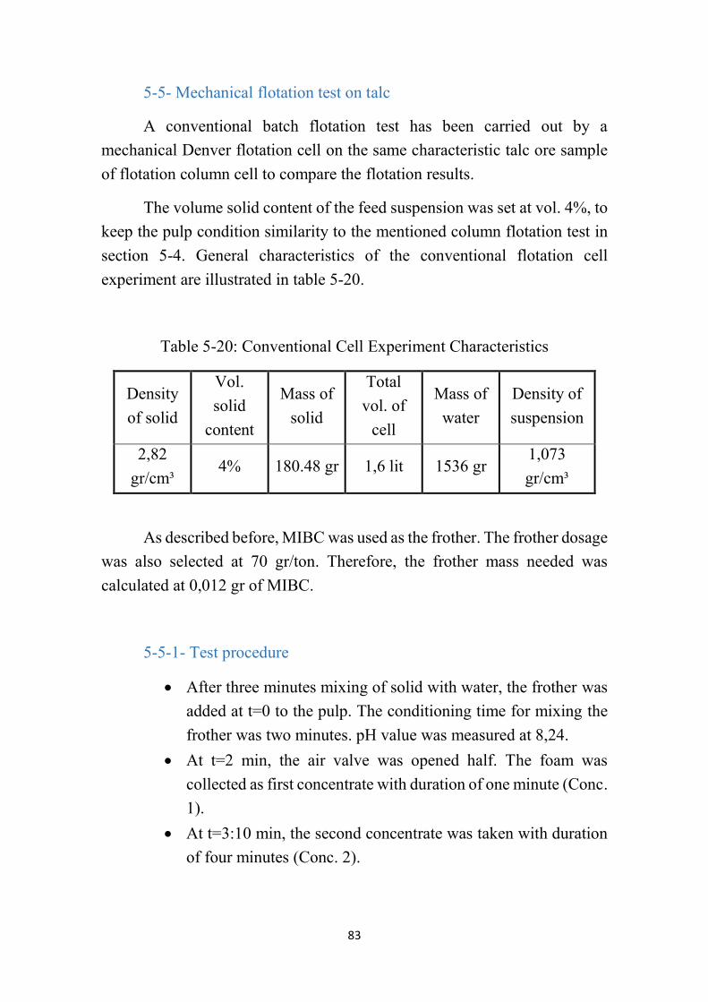
83
5-5- Mechanical flotation test on talc
A conventional batch flotation test has been carried out by a
mechanical Denver flotation cell on the same characteristic talc ore sample
of flotation column cell to compare the flotation results.
The volume solid content of the feed suspension was set at vol. 4%, to
keep the pulp condition similarity to the mentioned column flotation test in
section 5-4. General characteristics of the conventional flotation cell
experiment are illustrated in table 5-20.
Table 5-20: Conventional Cell Experiment Characteristics
Density
of solid
Vol.
solid
content
Mass of
solid
Total
vol. of
cell
Mass of
water
Density of
suspension
2,82
gr/cm³ 4% 180.48 gr 1,6 lit 1536 gr
1,073
gr/cm³
As described before, MIBC was used as the frother. The frother dosage
was also selected at 70 gr/ton. Therefore, the frother mass needed was
calculated at 0,012 gr of MIBC.
5-5-1- Test procedure
After three minutes mixing of solid with water, the frother was
added at t=0 to the pulp. The conditioning time for mixing the
frother was two minutes. pH value was measured at 8,24.
At t=2 min, the air valve was opened half. The foam was
collected as first concentrate with duration of one minute (Conc.
1).
At t=3:10 min, the second concentrate was taken with duration
of four minutes (Conc. 2).
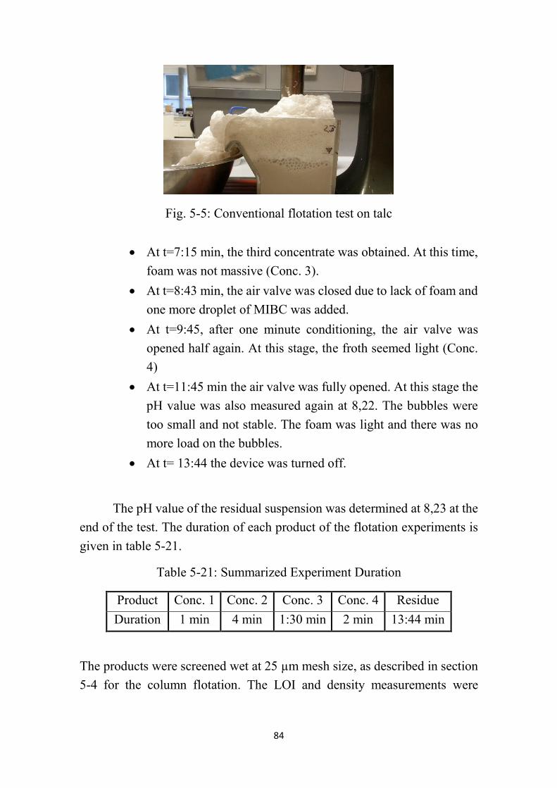
84
Fig. 5-5: Conventional flotation test on talc
At t=7:15 min, the third concentrate was obtained. At this time,
foam was not massive (Conc. 3).
At t=8:43 min, the air valve was closed due to lack of foam and
one more droplet of MIBC was added.
At t=9:45, after one minute conditioning, the air valve was
opened half again. At this stage, the froth seemed light (Conc.
4)
At t=11:45 min the air valve was fully opened. At this stage the
pH value was also measured again at 8,22. The bubbles were
too small and not stable. The foam was light and there was no
more load on the bubbles.
At t= 13:44 the device was turned off.
The pH value of the residual suspension was determined at 8,23 at the
end of the test. The duration of each product of the flotation experiments is
given in table 5-21.
Table 5-21: Summarized Experiment Duration
Product Conc. 1 Conc. 2 Conc. 3 Conc. 4 Residue
Duration 1 min 4 min 1:30 min 2 min 13:44 min
The products were screened wet at 25 µm mesh size, as described in section
5-4 for the column flotation. The LOI and density measurements were

85
included, in order to characterize the flotation products. The mass balance
table is developed in table 5-22.
Table 5-22: Mass balance table for conventional cell experiment on talc
Sample
Mass
(gr)
Float
mass
(%)
Washed
wet at 25
(µm)
Mass
(gr)
Mass in
fraction
(%)
Mass
Recovery
of Coarse
and Fine
(%)
Density
(gr/cm³)
Density
in
product
(gr/cm³)
LOI in
Fraction
(%)
LOI in
product
(%)
100- LOI (%
)
Mass
in
Feed
(%)
(100-LOI)
Recovery (%)
(100-LOI)
Recovery in
Product (%)
Cum.
Mass
Recovery
(%)
+2512,7
22,8036,05
2,8025,27
7,1828,27
-2542,99
77,2030,36
2,8186,61
24,3120,71
+259,39
18,5226,65
2,8145,16
5,3120,44
-2541,3
81,4829,16
2,816,23
23,3518,76
+251,72
21,744,88
2,8895,51
0,974,00
-256,19
78,264,37
2,8076,42
3,502,90
+255,93
27,9316,83
2,8185,20
3,3513,02
-2515,3
72,0710,80
2,8146,75
8,657,52
+255,49
13,2915,58
2,69514,79
3,1034,28
-2535,83
86,7125,30
2,75219,19
20,2650,11
+2535,23
19,92100,00
2,7956,73
-25141,61
80,08100,00
2,7989,69
31,49
60,16
64,63
76,63
100,00
32,46
29,63
4,61
12,37
20,92
93,70
93,97
93,78
93,69
2,814
2,811
2,825
2,815
6,30
6,03
6,22
6,31
31,492
28,664
4,473
12,005
23,366
Conc. 1
Conc. 2
Conc. 3
55,69
50,69
7,91
21,23
41,32
Conc. 4
Tail
9,1090,90
2,744
Feed176,8
1002,798
18,6081,40
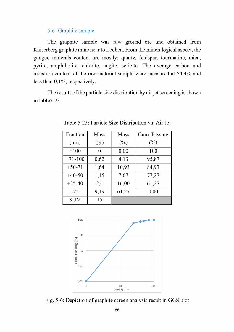
86
5-6- Graphite sample
The graphite sample was raw ground ore and obtained from
Kaiserberg graphite mine near to Leoben. From the mineralogical aspect, the
gangue minerals content are mostly; quartz, feldspar, tourmaline, mica,
pyrite, amphibolite, chlorite, augite, sericite. The average carbon and
moisture content of the raw material sample were measured at 54,4% and
less than 0,1%, respectively.
The results of the particle size distribution by air jet screening is shown
in table5-23.
Table 5-23: Particle Size Distribution via Air Jet
Fraction
(µm)
Mass
(gr)
Mass
(%)
Cum. Passing
(%)
+100 0 0,00 100
+71-100 0,62 4,13 95,87
+50-71 1,64 10,93 84,93
+40-50 1,15 7,67 77,27
+25-40 2,4 16,00 61,27
-25 9,19 61,27 0,00
SUM 15
Fig. 5-6: Depiction of graphite screen analysis result in GGS plot
0,01
0,1
1
10
100
1 10 100
Cu
m. P
assi
ng
(%)
Size (µm)

87
Table 5-24 is also shown the carbon concentration of the size fraction.
Table 5-24: Carbon Content in Size Classes
Fraction
(µm)
Mass
(%)
Carbon
Content
(%)
Carbon
Recovery
(%)
+100 0 0 0,00
+71-100 4,13 63,53 4,83
+50-71 10,93 58,45 11,75
+40-50 7,67 55,13 7,78
+25-40 16 53,66 15,79
-25 61,27 53,12 59,86
SUM 100 54,37 100
5-7- First graphite flotation test
The experiment was implemented by the column flotation cell on the
graphite ore sample with the properties mentioned in section 5-6. The
operation conditions are illustrated in table 5-25.
Table 5-25: Graphite Sample Operation Condition
The feed and wash water flowrates were 3,5 lit/min and 0,33 lit/min,
respectively. Therefore, the underflow discharge to keep the pulp level
constant was 3.83 lit/min.
Vol. Mass
Preparation of Suspension
Conditioning
Tank Vol.
Vol. Solid
Content
Solid
Densit
Solid Mass
of
Pulp
Densit
Retention
Time (sec)
1,059
gr/cm³16050 lit 4%
2,47
gr/cm³
0,002
m³
4950
gr
4800
gr
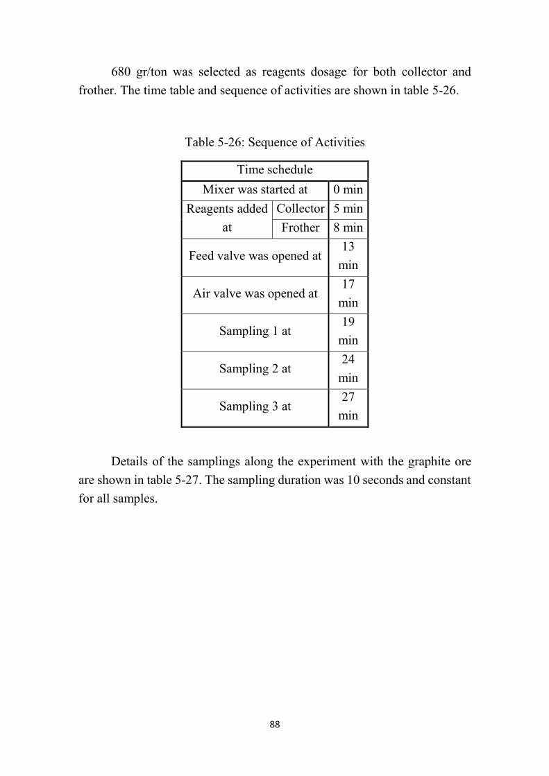
88
680 gr/ton was selected as reagents dosage for both collector and
frother. The time table and sequence of activities are shown in table 5-26.
Table 5-26: Sequence of Activities
Time schedule
Mixer was started at 0 min
Reagents added
at
Collector 5 min
Frother 8 min
Feed valve was opened at 13
min
Air valve was opened at 17
min
Sampling 1 at 19
min
Sampling 2 at 24
min
Sampling 3 at 27
min
Details of the samplings along the experiment with the graphite ore
are shown in table 5-27. The sampling duration was 10 seconds and constant
for all samples.

89
Table 5-27: Sampling details of first graphite experiment
Sample Name
Mass of
Suspension
(gr)
Mass of
Dry solid
(gr)
Sam. 1 Conc 103,26 10,83
Sam. 1 Tail 180,24 2,91
Sam. 2 Conc 76,84 8,46
Sam. 2 Tail 127,06 16,47
Sam. 3 Conc 198,67 17,49
Sam. 3 Tail 383,08 21,08
The experiment was run at slightly more than 0,3 bar compressed air
pressure. The gas holdup height difference was measured at 10,5 cm in
average, which led to 13,1 % gas holdup.
Table 5-28: Measured parameters of experiment
Parameter Value Unit
Difference height in gas holdup hose 10,5 cm
Gas holdup 13,1 %
Collection zone height 152,5 cm
Cleaning zone height 29,3 cm
Sampling duration 10 sec
Carrying capacity rate 0,023 gr/sec/cm²
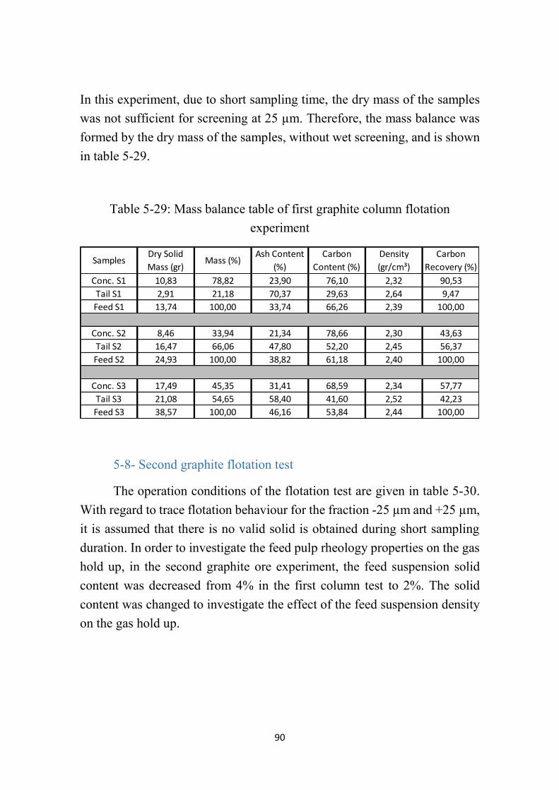
90
In this experiment, due to short sampling time, the dry mass of the samples
was not sufficient for screening at 25 µm. Therefore, the mass balance was
formed by the dry mass of the samples, without wet screening, and is shown
in table 5-29.
Table 5-29: Mass balance table of first graphite column flotation
experiment
5-8- Second graphite flotation test
The operation conditions of the flotation test are given in table 5-30.
With regard to trace flotation behaviour for the fraction -25 µm and +25 µm,
it is assumed that there is no valid solid is obtained during short sampling
duration. In order to investigate the feed pulp rheology properties on the gas
hold up, in the second graphite ore experiment, the feed suspension solid
content was decreased from 4% in the first column test to 2%. The solid
content was changed to investigate the effect of the feed suspension density
on the gas hold up.
SamplesDry Solid
Mass (gr)Mass (%)
Ash Content
(%)
Carbon
Content (%)
Density
(gr/cm³)
Carbon
Recovery (%)
Conc. S1 10,83 78,82 23,90 76,10 2,32 90,53
Tail S1 2,91 21,18 70,37 29,63 2,64 9,47
Feed S1 13,74 100,00 33,74 66,26 2,39 100,00
Conc. S2 8,46 33,94 21,34 78,66 2,30 43,63
Tail S2 16,47 66,06 47,80 52,20 2,45 56,37
Feed S2 24,93 100,00 38,82 61,18 2,40 100,00
Conc. S3 17,49 45,35 31,41 68,59 2,34 57,77
Tail S3 21,08 54,65 58,40 41,60 2,52 42,23
Feed S3 38,57 100,00 46,16 53,84 2,44 100,00

91
Table 5-30: Graphite Column Experiment Operation Condition
Preparation of Suspension
Conditioning
Tank Vol.
Vol.
Solid
Content
Solid
Density
Solid Mass
of
Water
Pulp
Density
Retention
Time
(sec) Vol. Mass
50 lit 2% 2,47
t/m³
0,001
m³ 2.5 kg 49 kg
1,029
t/m³ 240
The column operation settings such as pulp level, wash water flowrate,
sequence of the test implementation and the cell control procedure were kept
the same as mentioned before for the talc ore and the first graphite ore
flotation test in sections 5-4 and 5-7. The reagents added to floathe the
graphite, were diesel and MIBC as collector and frother, respectively. The
collector and frother were added into the conditioning tank with three
minutes time difference.
The feed and wash water flowrates were 2,4 lit/min and 0,33 lit/min.
Therefore, the underflow discharge was 2,73 lit/min to keep the constant
pulp level in the column cell. The time schedule of activities are shown in
table 5-31.

92
Table 5-31: Time schedule of graphite experiment
Time schedule
Mixer is started at 0 min
Reagents added
at
Collector 3 min
Frother 6 min
Feed valve is opened at 9 min
Air valve opened at 14
min
Sampling 1 at 18
min
Sampling 2 at 24
min
Sampling 3 at 32
min
The details of the obtained samples are shown in table 5-32. The
sampling duration is 40 sec.

93
Table 5-32: Sampling Details of Graphite Experiment
Sample Name
Mass of
Suspension
(gr)
Mass of
Dry solid
(gr)
Sam. 1 Conc 487,61 55,44
Sam. 1 Tail 425,74 3,84
Sam. 2 Conc 802,7 24,6
Sam. 2 Tail 1250,07 38,64
Sam. 3 Conc 952,24 62,28
Sam. 3 Tail 1700,5 39,76
During this experiment, the injected compressed air pressure and the
gas holdup difference height were read at 0,3 bar and 11,5 cm, respectively.
Table 5-33: Charactristics of column experiment on graphite
Parameter Value Unit
Difference height in gas holdup hose 11,5 cm
Gas holdup 14,4 %
Collection zone height (ℎ𝑐) 154,5 cm
Cleaning zone height 27,5 cm
Interstitial velocity (U= ℎ𝑐/τ) 0,85 cm/sec
Slurry superficial velocity (Jsl) 0,86 cm/sec
Axial mixing coefficient E 29,04 cm²/sec

94
In table 5-33, the axial mixing coefficient (E) is calculated according
to the equations (28) and (29):
Ϭ𝑟2 = 2𝑁𝑑 − 2𝑁𝑑
2 [1 − 𝑒−1
𝑁𝑑] (36)
𝐸 = 𝑁𝑑 . 𝑢. ℎ𝑐 (37)
Where:
𝑁𝑑 ........ Dispersion number
The dispersion number and the axial mixing coefficient are
calculated as 0,22127 and 29,04 cm²/sec, respectively.

95
Table5-34: Mass balance table for the second graphite ore test
Sam
ples
Mass o
f
dry
solid
(gr)
Yield
in
samp
ling
series (%)
Den
sity o
f
dry
pro
du
cts
(gr/cm
³)
Fractio
n
(µm
) M
ass (gr)
Mass (%
)
Mass
Reco
very
of C
oarse
(%)
Mass
Reco
very
of F
ine
(%)
Ash
con
tent
(%)
Size
related
ash
recov
ery
(%)
Ash
con
tent
in
pro
du
ct
(%)
Carb
on
con
tent
(%)
Den
sity
(gr/cm
³)
Carb
on
Reco
very
(%)
+25
33
,33
56
,23
97
,10
21
,71
91
,28
2,2
7
-25
22
,11
37
,30
88
,61
32
,18
76
,24
2,3
6
+25
1,0
01
,68
2,9
06
9,4
78
,72
2,6
8
-25
2,8
44
,79
11
,39
78
,02
23
,76
2,6
8
+25
34
,32
57
,90
10
0,0
02
3,0
91
00
,00
2,2
8
-25
24
,95
42
,10
10
0,0
03
7,4
01
00
,00
2,3
9
+25
16
,86
26
,67
58
,18
29
,50
42
,54
2,3
1
-25
7,7
31
2,2
32
2,5
84
2,8
91
7,5
53
,11
+25
12
,12
19
,17
41
,82
55
,44
57
,46
2,4
8
-25
26
,51
41
,93
77
,42
58
,79
82
,45
2,5
3
+25
28
,99
45
,84
10
0,0
04
0,3
51
00
,00
2,3
8
-25
34
,25
54
,16
10
0,0
05
5,2
01
00
,00
2,6
6
+25
21
,80
21
,36
65
,82
23
,50
39
,56
2,2
8
-25
40
,50
39
,69
58
,75
34
,71
40
,87
2,3
6
+25
11
,32
11
,09
34
,18
69
,14
60
,44
2,5
6
-25
28
,44
27
,87
41
,25
71
,53
59
,13
2,6
3
+25
33
,12
32
,46
10
0,0
03
9,0
91
00
,00
2,3
7
-25
68
,94
67
,56
10
0,0
04
9,9
01
00
,00
2,4
7
97
,79
2,2
1
10
0,0
0
49
,97
50
,03
10
0,0
0
78
,83
21
,17
10
0,0
05
3,6
1
29
,15
69
,21
51
,61
42
,26
66
,29
70
,89
24
,20
74
,12
93
,53
25
,88
75
,80
29
,11
33
,71
57
,74
46
,39
70
,85
30
,79
48
,39
2,3
1
2,5
3
2,3
3
2,6
8
61
,10
38
,90
10
0,0
0
6,4
7
Co
nc. S1
Co
nc. S2
Tail S1
Tail S2
62
,28
38
,64
24
,60
3,8
4
55
,44
63
,23
2,4
41
02
,04
Feed Sam
. 3
Feed Sam
. 2
Feed Sam
.15
9,2
8
2,6
1
2,3
3
2,5
2
2,5
6
Tail S3
Co
nc. S3
10
0,0
0
38
,97
61
,03
10
0,0
0
39
,76

96
5-8-1- Residence time distribution determination
During the second column flotation test with the graphite ore, the
residence time was also measured by injection of a saturated salt solution as
an impulse tracer into the column. The solution was prepared by the
magnetic impeller at room temperature and injected with a syringe near to
the feed port into the cell. At the time of injection (t=0), the first sample was
taken from the underflow discharge. 26 more time dependent samples were
also obtained from the underflow of the cell with 7 seconds time interval
between samplings. An average, the sampling duration was also 7 seconds.
By means of the conductivity value, the concentration of tracer was followed
in the samples. The conductivity measurement apparatus was calibrated with
0,01 mol/lit potassium chloride solution, according to the device manual.
Fig. 5-7: Obtained samples for residence time distribution determination
Residence time distribution diagram and the results of the residence
time are shown in table 5-35 and fig. 5-8.

97
Table 5-35: Sampling information for residence time distribution
determination
Sequence
(j)
Time
(sec)
Conductivity
(µS/cm) 𝑡𝑗*𝐶𝑗*𝛥𝑡𝑗 𝐶𝑗*𝛥𝑡𝑗
(𝑡𝑗-
𝜏𝑗)²*𝐶𝑗*𝛥𝑡𝑗
1 0 363 0 2541 82669333,3
2 14 363 35574 2541 70334239,6
3 28 365 71540 2555 59320260,5
4 42 370 108780 2590 49590466,4
5 56 390 152880 2730 42228932,2
6 70 395 193550 2765 33683364
7 84 397 233436 2779 25810305,9
8 98 398 273028 2786 18903563,5
9 112 396 310464 2772 12958472,9
10 126 393 346626 2751 8132915,82
11 140 388 380240 2716 4426873,61
12 154 385 415030 2695 1874370,14
13 168 383 450408 2681 410392,031
14 182 381 485394 2667 7065,8183
15 196 378 518616 2646 646217,931
16 210 375 551250 2625 2304223,89
17 224 372 583296 2604 4956387,69
18 238 372 619752 2604 8647753,29
19 252 370 652680 2590 13288059,5
20 266 373 694526 2611 19144113,2
21 280 366 717360 2562 25429579,7
22 294 366 753228 2562 33078623,2
23 308 365 786940 2555 41617948,8
24 322 364 820456 2548 51108804,4
25 336 363 853776 2541 61542958
26 350 364 891800 2548 73315007,2
27 364 363 924924 2541 85680298,7
SUM 12825554 71106 831110531

98
Fig. 5-8: Residence time distribution diagram
The residence time, variance and relative variance were calculated
according to the equations in section 2-1-16. The results are shown in table
5-36.
Table 5-36: Calculated residence time, variance and relative variance
𝜏 Ϭ² Ϭ𝑟2
180 sec 11688 sec 0,36
5-8-2- Pulp density and gas holdup correlation
As discussed before, the gas holdup is one of the most important
parameters which has a direct effect on the froth carrying capacity and the
process performance. The gas holdup parameter depends on a variety of
parameters such as the sparger type, the gas consumption, the bubble size,
machine and operation condition and etc.
360
365
370
375
380
385
390
395
400
0 100 200 300 400
Co
nd
uct
ivit
y (m
S/cm
)
Time (sec)
RTD

99
Of course, all the parameters affecting the gas holdup are of interest,
however it needs more measurement facilities to keep stable conditions
during the process. In this investigation, only the effect of the feed slurry
density on the gas holdup is determined and shown in table 5-37. It is
important to mention that the effect of narrow variations in some variables,
such as the feed flowrate, the overflow rate or compressed air pressure
alterations, are not considered in this investigation.
Table 5-37: Measured feed slurry density against gas holdup
Slurry Density
(gr/cm³)
Gas holdup
(%)
1 15,6
1,073 11,2
1,059 13,1
1,029 14,4
Fig. 5-9: Correlation between gas holdup and slurry density
As it has been illustrated in fig 5-9, an equation is developed to
estimate the gas holdup value. The correlation coefficient is also determined
as R²=0,93.
y = -55,973x + 71,8R² = 0,933
0
2
4
6
8
10
12
14
16
18
0,98 1 1,02 1,04 1,06 1,08
Gas
ho
ldu
p (
%)
Slurry density (gr/cm³)
100
5-9- Discussion
As it is mentioned in talc sample ore description (section 5-2), the
flotation feed LOI was measured at 9,02%. In table 5-18, LOI values of the
flotation feed, obtained from the back calculation of the column flotation
products, vary from 7,6 to 9,75 and 9,58 for first, second and third series of
sampling, respectively. A comparison of the measured and the calculated
results in table 5-18 shows that the third series of sampling has the nearest
results to the nominal feed properties. Moreover, the grade of products and
LOI recovery of each series of samplings fluctuate. The mentioned
inconstancies, could be the reason for the instability in the column cell
operation conditions. In semi-batch processing systems as well as continuous
systems, the process stabilization is time dependent. In addition, the manual
settings adjustment of the air, the input and the output slurry flowrates are
time consuming and alter the solid content of the prepared feed suspension.
Therefore, the amount of feed suspension to perform a stable flotation test
should be increased.
In order to achieve more stable conditions, the application of pumps
for adjustment of input and output flowrates can be a solution to keep a
constant level of suspension in the cell.
Furthermore, the level of feed suspension in the conditioning tank is
constantly decreasing during flotation process implementation. The changes
of the suspension level in the conditioning tank, cause a differential pressure
and thus, suspension velocity alterations. This suspension velocity changes
affected the feed pulp flowrate caused instability in the operation conditions.
In the current setup, the feed pulp flowrate decreases with the flotation
duration.
The other reason for the inconstancy in column cell performance
might be the effect of a pre-flotation and mineral segregation in the
conditioning tank. Occurrence of this phenomena can change the
characteristics of the feed suspension during flotation. The dimension ratio
of the impeller and the conditioning tank in order to provide an improved
mixing environment during feeding is important to consider.

101
In the mechanical flotation test on the alc ore, which was performed at
the same operation conditions and same feed material of column flotation
test as the column test, the LOI of the concentrate was obtained at 6,17%
with a concentrate mass recovery at 60,16%. The comparison of the column
and conventional flotation results show, slightly higher concentrate purity of
column test than the conventional apparatus, although the obtained yield in
column was less than in the conventional cell.
According to the obtained results of the tracer experiment within the
saturated salt solution, the mean residence time is obtained at 180 second. At
the beginning of the experiment, the feed flowrate was set at 2,4 lit/min. The
calculated mean residence time from the tracer experiment is in good
agreement with the retention time from plug flow
6- Suggestion for improvement
The suggestions that are recommendations for improvements in this
section are based on the experience obtained during the current tests. The
aim of this work study was the construction of the simplest generation of a
flotation column cell. To increase experiments accuracy, the implementation
of more facilities is necessary. As it has been shown in mass balance tables,
a fluctuation is obvious in the products grade and recovery. By slurry
discharging from conditioning tank, which is placed on the upper floor, the
feed flowrate is changed during flotation test due to pressure alteration. In
addition, pulp level adjustment in the column is carried out by manual feed
and discharge valves manipulation, which is not easy to perform and
accurate. It is also time consuming.
a) To achieve stable operation conditions for a semi-batch processing
system, a constant level of different parameters such as feed slurry flowrate
is needed. The flowrate of input streams and output stream must be equal to
have a constant level of suspension in the column cell. It is recommended,
as applied in commercial laboratory column flotation cells, to apply two
peristaltic pumps with the same properties for feed and underflow streams.
The most common used pump for laboratory column cells is the peristaltic
pump. They are more comfortable for low flowrates adjustments.

102
b) Feed pulp conditioning has also an important effect on the column
performance from two points of view. In some cases, due to high density
difference of minerals, mineral segregation during conditioning may occur.
The impeller design and rotational speed needs more investigation to
improvement. Another points to mention concern the conditioning tank
volume. A continuous experiment needs more time to reach to stable
conditions. Manual settings are also time consuming and waste the prepared
feed suspension before flotation commence. Therefore, the conditioning tank
must have the capacity for process stabilization.
c) Air flowmeter to measure air volume consumption during the
experiment is of advantage for further flotation parameters evaluation. This
measurement leads to calculate more parameters of the column such as gas
superficial velocity and carrying capacity of bubbles. These equipment must
be sensible enough for a laboratory device settings.
d) As it is observed by the author of this investigation work, narrow
alterations of compressed air pressure influence the bubble rise velocity and
flotation performance significantly. The range of the compressed air
alterations depend on the pulp rheology properties, suspension solid content
and pulp density.
e) The wash water flowrate and the bias rate influenced on the bubble
carrying capacity and the concentrate grade. It is recommended to investigate
optimum bias rate and wash water flowrate.
f) The kinetics of flotation is an effective parameter to achieve to the
stable conditions.

103
References:
1. M. C. Fuerstenau, G. Jameson, R. H. Yoon, Froth Flotation; A Century of
Innovation, SME, pp: 69-71.
2. J. B. Yianatos, Column Flotation Modelling and Technology, Chemical
Engineering Department, University of Santa Maria, Valparaiso, Chile,
pp: 1-31
3. A, Mular , D.N. Halbe, D.J. Barratt, Mineral Processing Plant, Design,
Practice and Control, Vol. I, SME, 2002, pp: 1097-1140.
4. S. Chander, R. R. Klimpel, Advances in Coal and Mineral Processing
Using flotation, Society for Mining, Metallurgy and Exploration Inc.,
1989, pp: 347-355
5. http://www. metso.com /products/separation/microcell-high-recovery-
flotation-columns/
6. S.K. Biswal, Flotation Column: A Novel Technique in Mineral
Processing.
7. R. R. Klimpel, (1995), “The influence of the frother structure on Industrial
Coal Flotation”, High- Efficiency Coal Preparation (Kawatra, ed.),
Society for Mining, Metallurgy and Exploration, Littleton, CO, pp. 141-
151
8. J.B. Rubinstein, Column Flotation Processes, Design and Practices.
Gordon and Breach Science Publishers, Institute of Solid Fuels
Preparation, Moscow, Russia, 1995, pp: 67-74,103-107, 181-190, 273-
276.
9. J.B. Yianatos, J.A. Finch and A.R. Lapante, Hold up profile and bubble
size determination of flotation column frothers, Canadian Metall.
Quarterly, 1986,25(1).

104
10. J.T. Furey, Rougher Column Flotation of Gold Tellurides. CMP Proc.
22nd Annual Meeting, 1990.
11. R. Espinoza- Gomez and N.W. Jamson, Technical Experience with
Conventional Columns at Mount Isa Mines Limited, Column 91,
Proceeding of an International Conference on Column Flotation, (G.A.
Agar, B.J. Huls, and D.B. Hyma, eds.), Sudbury, Ontario, Canada,
June1991, pp: 511-524.
12. R.D. Villar, M. Gregoire and A. Pomerleau, Mineral Engineering, Vol.
12, Pergamon, 1991, No. 3, p. 291-308.
13. F.J. Tavera, R. Escudero, J. A. Finch, Gas Holdup in Flotation Column;
Laboratory Measurements, International Journal of Mineral Processing,
2001, p. 23-40
14. M. Xu, Sparger Study in Flotation Columns, Master Dissertation,
Department of Mining and Metallurgical Engineering, McGill
University, 1987, pp: 4-28, 44-56,
15. J.B. Yianatos, A.R. Levy, Estimation of Gas Holdup, Diameter and
Apparent Density of Mineralized Bubbles in Industrial Flotation
Columns, Department of Chemical Engineering, University Santa Maria,
Valparaiso, Chile.
16. J.A. Finch and G.S. Dobby, Column Flotation, Pergamon press, 1990.
17. J.A. Finch, Column Flotation: A Selected Review- Part IV: Novel
Flotation Devices, Mineral Engineering, pergamon, 1995, Vol. 8, No. 6,
pp.: 587-602.

105
18. Y.T, Shah,. et al; Design parameters estimations for bubble column
reactors, 1982, AIChE J. vo1.28 No.3, p.: 353- 363,
19. D.A. Wheeler, Column Flotation- the original column, 87th Annual
General Meeting, CIM Vancouver, 1985, Aug.
20. G.B. Wallis, One Dimensional Two-phase flow, McGraw-Hill, New
York, AlChE Journal, 1969, Chapter. 9.
21. J.F. Richardson and W.N. Zaki, Sedimentation and fluidisation: part I,
Department of Chemical Engineering, Imperial College, London, 1954,
Vol. 32, pp: 32-35,
22. D. Bhaga, Master Thesis, McGill University, Montreal, Canada, 1970.
23. G.J. Jameson, S. Nam and M. Moo Young, Physical factors affecting
recovery rates in flotation, Mineral Science Engineering Journal, 1977,
Vol. 9, No. 3.
24. S.R.S. Sastri, Technical Note: Carrying Capacity in Flotation Columns,
Pergamon, Mineral Engineering, 1996, Vol. 9, No. 4, p. 465-468.
25. M. Falutsu, and G.S. Dobby, Froth Performance in Commercial Sized
Flotation Columns, Mineral Engineering, Vol. 5, 1992, 5(10-12), pp:
1207-1223.
26. S.A. Flynn and E.T. Woodburn, Development of a Froth Model for Fine
Particles Beneficiation by Flotation, 1987, Transaction of Institution of
Mining and Metallurgy, 1987, Section C, 96, Dec., C96, C191 and C191-
C198.
27. R.M. Yoon, M.J. Mankosa, G.H. Luttrell, Design and Scale up Criteria
for Column Flotation, XVIII International Mineral Processing Congress,
Aus., IMM Sydney, Australia, 1993, 785.

106
28. R. Espinonza- Gomez, J.A. Finch, J.B. Yianatos, G.S. Dobby, Flotation
Column Carrying Capacity: particle Size and Density Effect, 1988,
Mineral Engineering, Vol. 1, pp: 77-79.
29. R. Espinonza- Gomez, J.A. Finch, J.B. Yianatos, Carrying Capacity
Limitations in Flotation Columns, In: K.V.S Sastry (ed.), Column
Flotation-88, Proceeding of International Symposium on Column
Flotation, Soc. of Mining Engineering (SME), Littleton, CO, 1988,
pp:143-148.
30. R. Perez Garibay, A.P.M. Gallegos, S A. Uribe, A F. Nava, Effect of
Collection Zone Height and Operating Variables on Recovery of
Overload Flotation Columns, Mineral Engineering Journal, 2002, 15, p.:
325-331
31. K.S. Kawatra, T.C. Eisele, Flotation Column Design for Coal Phosphate
Processing. In: Proceeding of IX Congreso Internacional de Metalurgia
Extrativa., Universidad de Sonora, Mexico, 1999, p.: 43-66.
32. I.I. Maksimov, A.D. Borkin, M.F. Emelyanov, The Use of Column
Flotation machines for Cleaning Operations in Concentrating non-
ferrous Ores. In: Proceeding of XVII International Miner Processing
Congress, Dresden, FRG, Vol. 2, p.: 273-281.
33. A.Roberts, Mineral Processing, Proceeding of the Sixth International
Congress, Cannes, 1963, May 26- June 2, pp: 595-601
34. D. Lelinski, J. Allen, L. Redden, A. Weber, Analysis of the residence
time distribution in large flotation machines, Mineral Engineering, 15,
2002, pp: 499-505

107
35. B. Oteyaka, H. Soto, Air Velocity and Turbulence Effects in Flotation,
Pres. 33rd , Annual Conference of Metallurgists, The Metallurgical
Society of CIM, Toronto, Aug. 1994, pp: 20-25.
36. Z.A. Zhou, Z. Xu, J.A. Finch, Minimum Recovery Zone Height
Requirements in Flotation Columns from Particle- Bubble Collision
Analysis, Submitted to Mineral Eng., Vol. 104, 1995, pp: 102-106.
37. M.K. Ityokumbul, Design and Scale up issues in Column Flotation,
Innovations of Mineral Processing, Acme Printers, Sudbury, Canada,
1994, pp: 187-200.
38. J.B. Yianatos, J.A. Finch, G.S.Dobby and A.R. Lapante, Effect of
Column Height on Flotation Column Performance, Mineral and
Metallurgical Process, 1988, pp: 11-14.
39. R. del Villar, A. Desbiens, J.F. Huard, J. Bouchard, F.O. Verret, An
Experimental Set-up for the Study of Flotation Column Optimization,
University of Laval, Quebec, Canada.
40. G.G. Roy, R. Shekher, S.P. Mehrotra, Particle Suspension in (air
agitated) Pachuca Tanks, Metallurgical and Material Transactions, 1998,
29 (B), 339-349.
41. J.A. Finch, J. Xiao, C. Hardie, C.O. Gomez, Gas Dispersion Properties:
Bubble Surface Area Flux and Gas Holdup, Mineral Eng. Journal, Vol.
13, No. 4, 2000, pp: 365-372.
42. S. Banisi, J.A. Finch, Technical note: Reconciliation of Bubble Size
Estimation Methods using Drift Flux Analysis, Mineral Engineering,
1994, 7(12), pp: 1555-1559
43. R. J. King, Mineral Explained, No. 2, Graphite, Blackwell Publishing,
Geology today, Vol. 22, 2006, pp: 71- 77.
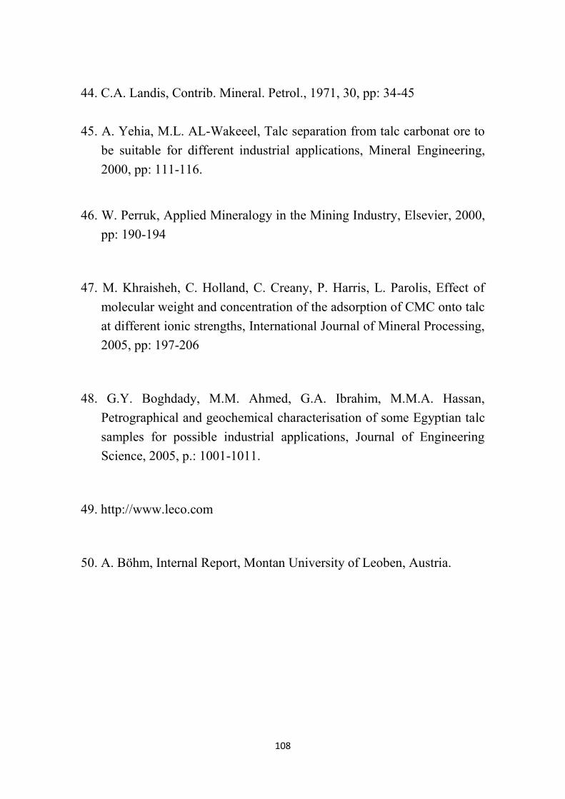
108
44. C.A. Landis, Contrib. Mineral. Petrol., 1971, 30, pp: 34-45
45. A. Yehia, M.L. AL-Wakeeel, Talc separation from talc carbonat ore to
be suitable for different industrial applications, Mineral Engineering,
2000, pp: 111-116.
46. W. Perruk, Applied Mineralogy in the Mining Industry, Elsevier, 2000,
pp: 190-194
47. M. Khraisheh, C. Holland, C. Creany, P. Harris, L. Parolis, Effect of
molecular weight and concentration of the adsorption of CMC onto talc
at different ionic strengths, International Journal of Mineral Processing,
2005, pp: 197-206
48. G.Y. Boghdady, M.M. Ahmed, G.A. Ibrahim, M.M.A. Hassan,
Petrographical and geochemical characterisation of some Egyptian talc
samples for possible industrial applications, Journal of Engineering
Science, 2005, p.: 1001-1011.
49. http://www.leco.com
50. A. Böhm, Internal Report, Montan University of Leoben, Austria.

109
Appendix 1: Foam Launder

110
Appendix 2: Main Upper Part

111
Appendix 3: Feed Port

112
Appendix 4: Assembled Feed Port on the Body of Cell
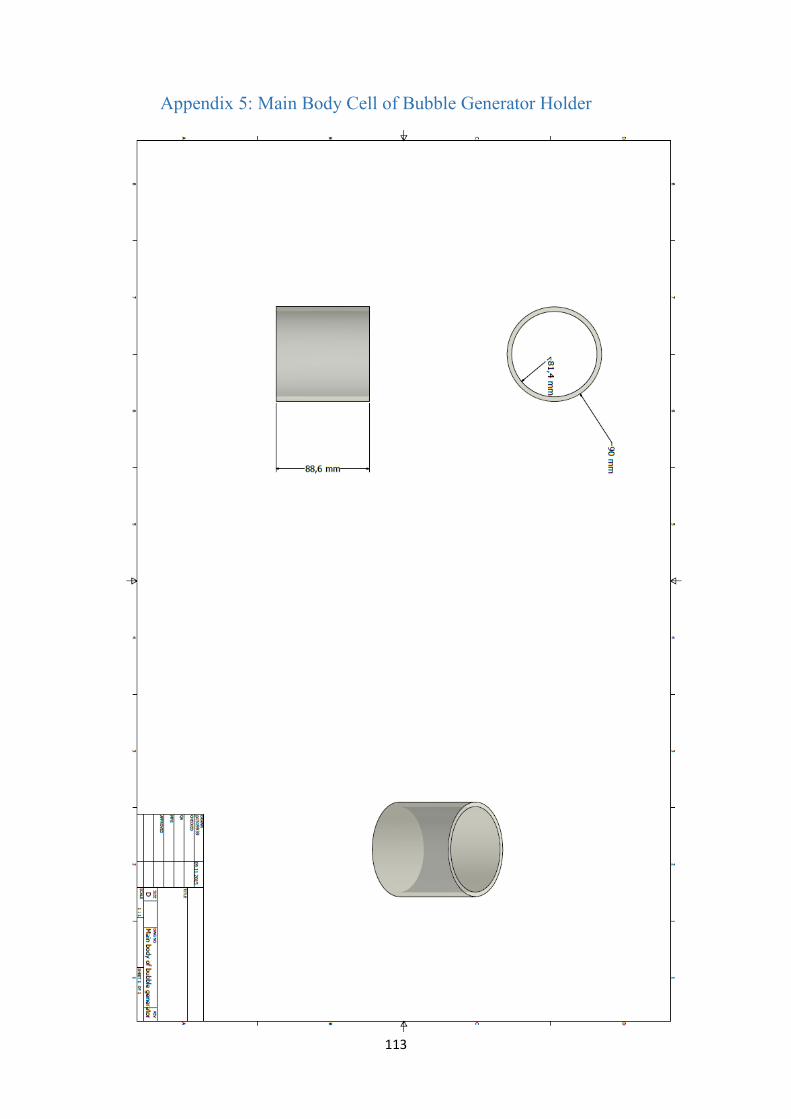
113
Appendix 5: Main Body Cell of Bubble Generator Holder
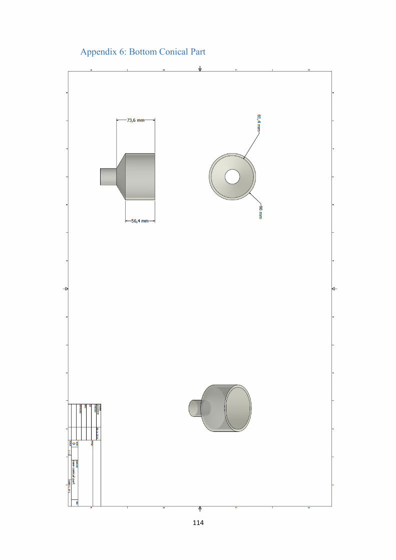
114
Appendix 6: Bottom Conical Part
115
Appendix 7: Bubble Generator Holder

116
Appendix 8: Assembled Flotation Cell

117
Appendix 9: Details of applied parts
Part Name Material Code d D L L1
Flanged
bushings
PVC-U 721 790 113 90
mm
108
mm
56
mm
11
mm
Part Name Material Code d
Union nut PVC-U 161 490 546 110 mm
Part Name Material Code d e Di
Pipe PVC-U 192 017 088 90
mm
4,3
mm
81,4
mm