design of a short to medium range hybrid transport aircraft · 2020-03-06 · design of a hybrid...
TRANSCRIPT

Design of a Short to Medium Range
Hybrid Transport Aircraft
A Project Presented to The Faculty of the Department of Aerospace Engineering
San José State University
In Partial Fulfillment of the Requirements for the Degree Master of Science in Aerospace Engineering
by
Sarah M. Ortega
approved by
Dr. Nikos J. Mourtos Faculty Advisor

Design of a Hybrid Transport Aircraft ii
Nomenclature
A = aspect ratio A/C = aircraft AEP = airplane estimated price Ah = horizontal tail aspect ratio 𝐴"#$ = capture area per inlet in square feet Av = vertical tail aspect ratio ac = aerodynamic center AHj = number of flight hours per year for crew member j ASP = avionics systems price b = wingspan B.L. = wing buttock lines CL = lift coefficient CD = drag coefficient Cr = cruise c = chord cr = root chord ct = tip chord CGR = climb gradient cg = center of gravity C&'( = control power derivative C)*+/*- = labor cost of airframe and system maintenance C)*+/.&/ = labor cost of engine maintenance C0*1/*- = cost of maintenance materials for the airframe and systems C0*1/.&/ = cost of maintenance materials for the engines C*0+ = applied maintenance burden 𝐶345 = cost of airplane depreciation 𝐶36#7 = cost of engine depreciation 𝐶348 = cost of avionics system depreciation 𝐶34595 = cost of airplane spare parts depreciation 𝐶36#795 = cost of engine spare parts depreciation Clf = direct operating cost due to landing fees Caplf = airplane landing fee per landing Cnf = navigation fee Capnf = navigation fee charged per airplane per flight Crt = direct cost of registry taxes DOC = direct operating cost DOClnr = direct operating cost of landing fees DOCfin = direct operating cost of financing the airplane DPap = airplane depreciation period DPav = airplane avionics system depreciation period DPengsp = depreciation period for engine spare parts e = battery specific energy, Oswald constant Ebat = energy of batteries E; = propulsive energy required

Design of a Hybrid Transport Aircraft iii
EP = engine price ESPPF = engine spare parts price factor Fdap = airframe depreciation factor Fdav = airplane avionics system depreciation factor f = equivalent parasite area F.S. = fuselage stations FAA = Federal Aviation Administration FAR = Federal Aviation Regulations FT = Fischer-Tropsch Fengsp = engine spare parts factor frt = factor depending on airplane size g = gravitational acceleration h = height ℎ=>9 = height of fuselage in feet HTA = Hybrid Transport Aircraft iw = incidence angle j = crew member type K = drag due to lift polar coefficient Kg = gust alleviation factor kj = factor accounting for crew vacation pay, cost of training crew insurance, etc. LE = leading edge LG = landing gear Ltr = loiter 𝑙=>9 = length of fuselage in feet 𝑙@ = distance from wing root quarter cord to horizontal tail quarter cord in ft 𝑙# = nacelle length n = load factor 𝑛BC = number of crew members of type j ND = drag induced yawing moment 𝑁6 = number of engines 𝑛$"EFGH = positive limit naneuvering load factor 𝑛$"EIJK = negative limit naneuvering load factor 𝑁"#$ = number of inlets 𝑁54L = number of passengers 𝑁5"$ = number of pilots mgc = mean geometric chord MH = maximum Mach number at sea level Mff = mission fuel fraction Mres = reserve fuel fraction Mtfo = trapped fuel fraction MEA = More Electric Aircraft p = battery specific power Pr = power required (propulsive) 𝑃N = maximum static pressure at engine compressor face in psi q = dynamic pressure in psf 𝑞P = design dive dynamic pressure in psf

Design of a Hybrid Transport Aircraft iv
RC = rate of climb Rer = Reynold’s number at root chord Ret = Reynold’s number at chord tip 𝑅R$ = block distance 𝑅B$ = climb distance 𝑅36 = descent distance 𝑅E4# = maneuvering distance S = wing reference surface area Sh = horizontal tail area Sv = vertical tail area S = gross wing area SALj = yearly salary per crew member STOFL = takeoff field length T = time of flight Tphase = time of flight for a certain phase TBW = Truss Braced Wing t/c = thickness ratio Tcl = time to climb T/W = thrust loading (or thrust to weight ratio) 𝑡TU = horizontal tail maximum root thickness 𝑡TV = vertical tail maximum root thickness TEFj = travel expense factor per crew member j W/S = Wing loading 𝑊4" = air induction system weight 𝑊45" = weight of air-conditioning, pressurization, anti-icing and de-icing system 𝑊45> = weight of auxiliary power unit (APU) Wbat = weight of batteries 𝑊RB = weight of baggage and cargo handling equipment We = empty weight 𝑊6$9 = weight of electrical system 𝑊6#7 = weight of engine Wf = fuel weight 𝑊=B = weight of flight control system 𝑊=>T = weight of furnishings 𝑊@9 = weight of hydraulic and pneumatic system 𝑊" = weight of instruments 𝑊"46 = weight of the instrumentation, avionics, and electronics Woe = operating empty weight 𝑊X59 = weight of operational items 𝑊XL = weight of oxygen system Wpl = payload weight 𝑊5Y = weight of paint Wtfo = trapped fuel weight Wto = take off weight WL = landing weight 𝑊=9 = fuel system weight

Design of a Hybrid Transport Aircraft v
𝑊=>9 = weight of fuselage in lbs 𝑤=>9 = width of fuselage 𝑊5 = propulsion system 𝑊5[T = powerplant weight 𝑊9YT>BY = weight of structure 𝑈4##]^ = annual utilization in block hours V = velocity VB = design speed for maximum gust intensity VA = approach speed VC = design cruise speed Vcr = cruise velocity VD = design diving speed VM = design maneuvering speed 𝑉54L = passenger cabin volume VS = +1g stall speed or minimum speed at which airplane is controllable 𝑥8, 𝑥@,𝑥B = distance from center of gravity to aerodynamic center of the surface yt = lateral thrust moment arm of most critical engine zh = distance from vertical tail to root, where horizontal tail is mounted on vertical tail ηp = propeller efficiency 𝜌 = air density Λ = quarter chord sweep angle λ = taper ratio εw = twist angle Γw = dihedral angle

Design of a Hybrid Transport Aircraft vi
Table of Contents
Nomenclature .................................................................................................................. ii
List of Figures ............................................................................................................... xv
List of Tables ................................................................................................................. xx
1. Introduction ................................................................................................................. 1
1.1. Exploring Hybrid Possibilities for the Next Generation of Transport Aircraft ........ 1
1.1.1. Environmental Factors ................................................................................... 1
1.2 Alternate Fuel Sources ........................................................................................... 2
1.2.1. Synthetic Fuel ................................................................................................ 2
1.2.2. Hydrocarbon Feedstock .................................................................................. 3
1.2.3. Alternative Fuel Comparisons...................................................................... 3
1.2.4. Lithium Ion Batteries ................................................................................... 3
1.3. Battery Sizing ....................................................................................................... 5
1.4. Project Objective ............................................................................................ 10
1.5. Mission Specifications ....................................................................................... 11
1.5.1. Mission Specifications ................................................................................. 11
1.5.2. Mission Profile ............................................................................................. 11
1.6. Methodology ...................................................................................................... 12
1.7. Comparative Study of Airplanes with Similar Mission Performance................... 12

Design of a Hybrid Transport Aircraft vii
1.7.1. Comparison of Weights, Performance, and Geometries of Similar Airplanes 12
1.7.2. Configuration Comparison of Similar Airplanes ........................................... 15
1.8. Discussion .......................................................................................................... 20
2. Configuration Selection ......................................................................................... 23
2.1. Overall Configuration ......................................................................................... 23
2.1.1. Fuselage Configuration ................................................................................ 23
2.1.2. Engine Configuration ................................................................................... 24
2.1.3. Wing Configuration ...................................................................................... 24
2.1.4. Empennage Configuration ............................................................................ 25
2.1.5. Landing Gear Configuration ......................................................................... 25
3. Weight Sizing and Weight Sensitivities .................................................................. 26
3.1 Data Base for Takeoff Weights and Empty Weights of Similar Airplanes .............. 26
3.2. Determination of Mission Weights ...................................................................... 28
3.3. Manual Calculation of Mission Weights .............................................................. 29
3.3.1. Payload Weight ............................................................................................ 29
3.3.2. Estimated Takeoff Weight Method 1 ............................................................. 29
3.3.3. Determination of Mission Fuel Weight ......................................................... 30
3.3.4. Estimating Takeoff Weight Method 2 ........................................................... 33
3.3.5. Determining Allowable Value for Empty Weight .......................................... 34

Design of a Hybrid Transport Aircraft viii
3.3.6. Determination of Mission Battery Weight..................................................... 36
3.4. AAA Calculation of Mission Weights .................................................................. 37
3.5.Takeoff Weight Sensitivities ................................................................................. 39
3.5.1. Manual Calculations of Takeoff Weight Sensitivities .................................... 39
3.5.2. AAA Calculation of Takeoff Weight Sensitivities ........................................ 42
3.6. Trade Studies ...................................................................................................... 43
3.7. Takeoff Weight vs. Critical Mission Parameters .................................................. 44
3.7.1. Takeoff Weight vs. L/D ................................................................................ 44
3.7.2. Takeoff Weight vs. Payload .......................................................................... 45
3.7.3. Takeoff Weight vs. Range ............................................................................. 45
3.7.4. Takeoff Weight vs. Specific Fuel Consumption ............................................ 46
3.8. AAA Calculation of Range vs. Payload ............................................................... 47
3.9. Trade Study Conclusions..................................................................................... 47
4. Determination of Performance Constraints ............................................................. 48
4.1. Manual Calculation of Performance Constraints.................................................. 49
4.1.1. Stall Speed Sizing ........................................................................................ 49
4.1.2. Takeoff Distance Sizing ............................................................................... 49
4.1.3. Landing Distance Sizing .............................................................................. 52
4.1.4. Climb Requirement Sizing ........................................................................... 54

Design of a Hybrid Transport Aircraft ix
4.1.5. Maneuvering Requirement Sizing ................................................................ 57
4.1.6. Cruise Speed Requirement Sizing ................................................................ 57
4.2. AAA Calculation of Performance Constraints ..................................................... 58
4.2.1. Stall Speed Sizing ........................................................................................ 58
4.2.2. Takeoff Distance Sizing ............................................................................... 58
4.2.3. Landing Distance Sizing .............................................................................. 58
4.2.4. Climb Requirement Sizing ........................................................................... 59
4.2.5. Cruise Speed Requirement Sizing ................................................................ 59
4.2.6. Matching Plot............................................................................................... 59
5. Fuselage and Cockpit Design ..................................................................................... 60
5.1. Cockpit Design ................................................................................................... 60
5.1.1. Cockpit Layout Design................................................................................. 63
5.2. Fuselage Design .................................................................................................. 64
5.2.1. Fuselage Layout Design ............................................................................... 64
5.3. Recommendations and Conclusions .................................................................... 68
5.3.1. Recommendations ........................................................................................ 68
5.3.2. Conclusions ................................................................................................. 68
6. Wing, High-Lift System and Lateral Control Design .................................................. 69
6.1. Wing Planform Design ........................................................................................ 69

Design of a Hybrid Transport Aircraft x
6.1.1. Sweep Angle-Thickness Ratio Combination ................................................. 69
6.2. Airfoil Selection .................................................................................................. 71
6.3. Design of the High-Lift Devices ......................................................................... 72
6.3.1. AAA Calculation of Lift Coefficient ............................................................. 75
6.4. Design of the Lateral Control Surfaces ................................................................ 76
6.5. Drawings ............................................................................................................ 78
6.6. Discussion .......................................................................................................... 78
6.7. Recommendations and Conclusions .................................................................... 79
6.7.1. Recommendations ........................................................................................ 79
6.7.2. Conclusions ................................................................................................. 79
7. Design of the Empennage and the Longitudinal and Directional Controls .................. 80
7.1. Overall Empennage Design ................................................................................. 80
7.2. Design of the Horizontal Stabilizer ..................................................................... 81
7.3. Design of the Vertical Stabilizer .......................................................................... 81
7.4. Empennage Configuration Drawings ................................................................... 82
7.5. Empennage Design Evaluation............................................................................ 83
7.6. Discussion .......................................................................................................... 84
7.7. Recommendations and Conclusions .................................................................... 84
7.7.1. Recommendations ........................................................................................ 84

Design of a Hybrid Transport Aircraft xi
7.7.2. Conclusions ................................................................................................. 84
8. Design of the Landing Gear and Weight and Balance Analysis................................... 86
8.1. Introduction ........................................................................................................ 86
8.2. Estimation of the Center of Gravity ..................................................................... 86
8.3. Landing Gear Design .......................................................................................... 95
8.4. Weight and Balance ............................................................................................ 98
8.5. Conclusion .......................................................................................................... 98
9. Stability and Control Analysis ................................................................................... 98
9.1. Introduction ........................................................................................................ 98
9.2. Static Longitudinal Stability ................................................................................ 99
9.3. Static Directional Stability ................................................................................ 101
9.4. Minimum Control Speed with One Engine Inoperative ..................................... 102
9.5. Empennage Design-Weight and Balance- Landing Gear Design- Longitudinal
Static Stability and Control Check ....................................................................................... 103
9.7. Conclusion ........................................................................................................ 104
10. Drag Polar Estimation ............................................................................................ 104
10.1. Introduction .................................................................................................... 104
10.2. Airplane Zero Lift Drag .................................................................................. 104
10.3. Low Speed Drag Increments and Compressibility Drag .................................. 107

Design of a Hybrid Transport Aircraft xii
10.3.1. High Lift Device Drag Increments for Takeoff and Landing Gear Drag .... 108
10.5. Airplane Drag Polars ....................................................................................... 109
10.6. Discussion ...................................................................................................... 109
10.7. Conclusion ...................................................................................................... 110
11. Environmental and Economic Tradeoffs ................................................................. 110
11.1. Important Design Parameters .......................................................................... 110
11.2. Recommendations ........................................................................................... 111
11.2.2. Einvironmental/Economic Tradeoffs ........................................................ 111
12. Preliminary Design Sequence II ............................................................................. 111
13. V-n Diagram .......................................................................................................... 112
13.1. Calculation of VS ............................................................................................ 113
13.2. Calculation of VC ............................................................................................ 113
13.3. Calculation of VD ............................................................................................ 114
13.4. Calculation of VM ........................................................................................... 114
13.5. V-n Maneuver Diagram and V-n Gust Diagram ............................................... 116
14. Class II Weight and Balance .................................................................................. 117
14.1. Class I Weights ............................................................................................... 117
14.2. Weight Estimate Calculations .......................................................................... 118
14.2.1. Structural Weight ..................................................................................... 118

Design of a Hybrid Transport Aircraft xiii
14.2.2. Powerplant Weight ................................................................................... 123
14.2.3. Fixed Equipment Weight .......................................................................... 124
14.2.4. Empty Weight Discussion......................................................................... 135
14.3. Component Centers of Gravity ........................................................................ 136
14.4. Airplane Inertias.............................................................................................. 139
15. Cost Analysis ......................................................................................................... 139
15.1. Direct Operating Cost ..................................................................................... 141
15.1.1. Direct Operating Cost of Flying ............................................................... 142
15.1.2. Direct Operating Cost of Maintenance ...................................................... 143
15.1.3. Direct Operating Cost of Depreciation ...................................................... 145
15.1.4. Direct Operating Cost of Landing Fees, Navigation Fees, and Registry Taxes
........................................................................................................................................ 147
15.1.5. Direct Operating Cost of Financing .......................................................... 147
15.1.5. Direct Operating Cost Discussion ............................................................. 147
15.2. Indirect Operating Cost ................................................................................... 150
15.3. Program Operating Cost .................................................................................. 150
15.3. Hybrid Power Cost Analysis ........................................................................... 151
15.3.1. Sample Battery Specifications .................................................................. 151
16. Conclusion ............................................................................................................ 152

Design of a Hybrid Transport Aircraft xiv
References ................................................................................................................... 154

Design of a Hybrid Transport Aircraft xv
List of Figures
Figure 1. World Carbon Dioxide Emissions ................................................................................ 1
Figure 2. Direct CO2 emissions from 1 gallon of fuel (lbs/gal) .................................................... 2
Figure 3. Number of General Aviation Aircraft from 1970 to 2014 ............................................. 2
Figure 4. Alternative Biofuels ..................................................................................................... 3
Figure 5. Comparison of different types ...................................................................................... 4
Figure 6. Performance Comparison of Li-ion Batteries .............................................................. 4
Figure 7. Mission Profile Comparison of Sample Aircraft .......................................................... 8
Figure 8. Current and expected battery technology .................................................................... 10
Figure 9. Mission Profile ........................................................................................................... 11
Figure 10. Boeing 737-100 aircraft configurations (Boeing Commercial Airplanes, 2013)........ 15
Figure 11. Boeing 737-200 aircraft configuration. (Boeing Commercial Airplanes, 2013) ........ 16
Figure 12. Airbus A320NEO aircraft configuration (Airbus Commerial Aircraft, n.d.) .............. 17
Figure 13. Embraer ERJ-170-100 aircraft configuration (Jane's All the World's Aircraft, 2013) 18
Figure 14. CRJ200-ER aircraft configuration (Canadair Regional Jet, 2016) ............................. 19
Figure 15. SUGAR Volt 765-096 RevA aircraft configuration (Bradley & Droney, Subsonic
Ultra Green Aircraft Research: Phase II- Volume II- Hybrid Electric Design Exploration, 2015)
................................................................................................................................................. 20
Figure 16. Log-Log Plot of Takeoff Weight vs. Empty Weight with included trendline and linear
regression equation ................................................................................................................... 27
Figure 17. Regression Line Constants for Aircraft ..................................................................... 28
Figure 18. Weight Trends for Transport Jets .............................................................................. 36
Figure 19. AAA output with all fuel aircraft with 2 turbojet engines .......................................... 38

Design of a Hybrid Transport Aircraft xvi
Figure 20. We vs. Wto of 2 turbojet engine fuel-powered aircraft with ideal design point of
Wto=71,635.9 lbs and We=39,775.9 lbs ..................................................................................... 38
Figure 21. Takeoff weight sensitivities calculated by AAA for fuel-powered aircraft ................. 43
Figure 22. Takeoff weight sensitivities calculated by AAA for electric aircraft .......................... 43
Figure 23. Takeoff Weight vs. L/D for Cruise ............................................................................ 44
Figure 24. Takeoff Weight vs. L/D for Loiter............................................................................. 44
Figure 25. Takeoff Weight vs. Payload Weight (ranges from 80 passengers to 124 passengers) .. 45
Figure 26. Takeoff Weight vs. Range ......................................................................................... 45
Figure 27. Takeoff Weight vs. Specific Fuel Consumption during Cruise .................................. 46
Figure 28. Takeoff Weight vs. Specific Fuel Consumption during Loiter ................................... 46
Figure 29. Range vs. Payload .................................................................................................... 47
Figure 30. Range vs. Payload with design point Wpl=19,630.6 lb and Rcr=1,638.7 nm for fuel-
powered aircraft ........................................................................................................................ 47
Figure 31. AAA results of stall speed sizing .............................................................................. 58
Figure 32. AAA results of takeoff distance sizing ...................................................................... 58
Figure 33. AAA results of landing distance sizing ..................................................................... 59
Figure 34. AAA results of climb requirement sizing .................................................................. 59
Figure 35. AAA results of cruise speed requirement sizing ........................................................ 59
Figure 36. AAA results of the performance sizing plot .............................................................. 60
Figure 37. Dimensions of sitting male crew member in cockpit (Roskam, 2011). ...................... 61
Figure 38. Radial eye vectors emanating from C. (Roskam, 2011) ............................................. 62
Figure 39. Ideal minimum visibility pattern for transport aircraft. (Roskam, 2011) .................... 62

Design of a Hybrid Transport Aircraft xvii
Figure 40. Side and top-down view of cockpit. Dimensions in meters (Boeing Commercial
Airplanes, 2013) ....................................................................................................................... 63
Figure 41. Front and side 3-D view of cockpit. Dimensions in meters (Boeing Commercial
Airplanes, 2013) ....................................................................................................................... 63
Figure 42. Rear view of cockpit. (Aircraft Technical Data and Specifications: Boeing 737-
100/200, 2017) .......................................................................................................................... 64
Figure 43. Top down view of the fuselage (Boeing Commercial Airplanes, 2013) ..................... 64
Figure 44. Front view of the fuselage (Boeing Commercial Airplanes, 2013) ............................ 65
Figure 45. Front 3-D view of the 6 abreast passenger seating in the fuselage (Creative Aviation
Photography, 2017) ................................................................................................................... 65
Figure 46. Rear 3-D view of the 6 abreast passenger seating in the fuselage (Creative Aviation
Photography, 2017) ................................................................................................................... 66
Figure 47. Side view of fuselage with cargo compartment visible (Boeing Commercial Airplanes,
2013) ........................................................................................................................................ 67
Figure 48. Side view of fuselage with cargo placement (Boeing Commercial Airplanes, 2013) . 68
Figure 49. Jet Transports Wing Geometric Data (Roskam, Airplane Design Part II: Preliminary
Configuration Design and Integration of the Propulsion System, 2011) ..................................... 69
Figure 50. Plots of t/c and Ww vs. Λ .......................................................................................... 70
Figure 51. Boeing 737 Airfoil selections schematic (Aircraft Technical Data and Specifications:
Boeing 737-100/200, 2017) ....................................................................................................... 71
Figure 52. Cl vs. angle of attack for maximum lift coefficient at root and midspan .................... 73
Figure 53. Effect of Flap Chord Ratio and Flap Type on K ........................................................ 74
Figure 54. AAA Estimate of clean Lift Coefficient of the Wing ................................................. 75

Design of a Hybrid Transport Aircraft xviii
Figure 55. Wing Planform: flap and lateral control layout ......................................................... 78
Figure 56. Empennage Configuration (units in feet) .................................................................. 82
Figure 57. Horizontal Tail Geometry Calculations by AAA ....................................................... 83
Figure 58. Vertical Tail Geometry Calculations by AAA ........................................................... 83
Figure 59. Vertical tail configuration in HTA ............................................................................. 85
Figure 60. Horizontal tail configuration in HTA ........................................................................ 85
Figure 61. c.g. for various aircraft components .......................................................................... 88
Figure 62. c.g. location for each component on the aircraft ........................................................ 89
Figure 63. c.g. excursion plot produced using Microsoft Excel .................................................. 90
Figure 64. Weight fractions referenced from the 737-200 from AAA ......................................... 90
Figure 65. c.g. locations produced using AAA .......................................................................... 91
Figure 66. c.g. location for MTOW aircraft ............................................................................... 91
Figure 67. Loading Table from AAA for x-direction c.g. excursion diagram .............................. 92
Figure 68. c.g. excursion diagram (x-direction) ......................................................................... 93
Figure 69. Loading Table from AAA for z-direction c.g. excursion diagram .............................. 94
Figure 70. c.g. excursion diagram (z-direction) ......................................................................... 94
Figure 71. Landing gear and strut placement ............................................................................. 96
Figure 72. Nose gear retraction ................................................................................................. 96
Figure 73. Stick Diagram for main gear retraction ..................................................................... 97
Figure 74. Illustration of the two nose tires and four main tires for the landing gear. ................. 97
Figure 75. Landing Gear retracted into fuselage ........................................................................ 97
Figure 76. Geometric quantities for aircraft calculations .......................................................... 100

Design of a Hybrid Transport Aircraft xix
Figure 77. Longitudinal X-Plot for the HTA ............................................................................ 100
Figure 78. HTA Directional X-Plot .......................................................................................... 101
Figure 79. Geometry for one engine out Vmc calculations ........................................................ 102
Figure 80. Maximum takeoff weight vs. wetted area for jet transports ..................................... 106
Figure 81. Wetted area vs. equivalent parasite area .................................................................. 107
Figure 82. Typical Compressibility Drag Behavior .................................................................. 108
Figure 83. Low speed polars for transport ............................................................................... 109
Figure 84. L/D Ratios.............................................................................................................. 109
Figure 85. 3-view of HTA ....................................................................................................... 110
Figure 86. Ghost View of Aircraft ........................................................................................... 112
Figure 87. V-n Maneuver Diagram .......................................................................................... 116
Figure 88. V-n Gust Diagram .................................................................................................. 116
Figure 89. hFan engine overview ............................................................................................ 124
Figure 90. Class II c.g. Excursion Diagram ............................................................................. 138
Figure 91. DOC for a Jet Transport ......................................................................................... 148
Figure 92.HTA DOC with batteries and fuel ............................................................................ 148
Figure 93. HTA DOC for all fuel ............................................................................................. 149
Figure 94. Effect of variable depreciation period on DOC ....................................................... 149

Design of a Hybrid Transport Aircraft xx
List of Tables
Table 1. Preliminary database of Electric Aircraft ....................................................................... 5
Table 2. Mission Overview of Sample Aircraft ........................................................................... 8
Table 3. Summary of Theoretical Specific Energy ..................................................................... 10
Table 4. Comparison of Aircraft Weights ................................................................................... 12
Table 5.Comparison of Aircraft Performance (Assuming standard conditions at sea level) ........ 13
Table 6. Comparison of Aircraft Geometries ............................................................................. 14
Table 7. Aircraft Takeoff and Empty Weights ............................................................................ 26
Table 8. Data for Wto Comparison ............................................................................................. 30
Table 9. Suggested Fuel-Fractions for Mission Phases ............................................................... 31
Table 10. Breguet Partials for Propeller and Jet Airplanes ......................................................... 40
Table 11. Stall Speed Sizing ...................................................................................................... 49
Table 12. Takeoff Distance Sizing for STOFL =5000 ft at 0 ft altitude .......................................... 50
Table 13. Takeoff Distance Sizing for STOFL =6000 ft at 0 ft altitude .......................................... 51
Table 14. Takeoff Distance Sizing for STOFL =9468 ft at 5000 ft altitude .................................... 51
Table 15. Takeoff Distance Sizing for STOFL =10800 ft at 8000 ft altitude .................................. 51
Table 16. W/Sto with WL/Wto=0.85 ............................................................................................ 53
Table 17. W/Sto with WL/Wto=0.9 .............................................................................................. 53
Table 18. W/Sto with WL/Wto=0.93 ............................................................................................ 53
Table 19. W/Sto with WL/Wto=0.96 ............................................................................................ 54
Table 20. Configuration Parameters and Drag Polars ................................................................. 54
Table 21. FAR 25.111 (gears down, TO flaps, with additional T/W calculated for 50ºC increase)
................................................................................................................................................. 55

Design of a Hybrid Transport Aircraft xxi
Table 22. FAR 25.121 (gears down, TO flaps, with additional T/W calculated for 50ºC increase)
................................................................................................................................................. 55
Table 23. FAR 25.111 (gears down, TO flaps, with additional T/W calculated for 50ºC increase)
................................................................................................................................................. 56
Table 24. FAR 25.121 (gears up, flaps up, with additional T/W calculated for 50ºC increase and
maximum thrust at 0.94) ........................................................................................................... 56
Table 25. FAR 25.119 (AEO) (balked landing, gears down, flaps down) ................................... 56
Table 26. FAR 25.121 (OEI) (balked landing, gears down, flaps down) ..................................... 56
Table 27. Sizing to Time to Climb Requirements ...................................................................... 57
Table 28. Thickness Ratio and Wing Weight vs. sweep angle .................................................... 70
Table 29. ∆CLmaxTO and ∆CLmaxL using various Swf/S ......................................................... 74
Table 30. Calculated∆𝑐𝑙 for takeoff and landing ....................................................................... 75
Table 31. Jet Transport Lateral Control Surface Information...................................................... 76
Table 32. Additional Jet Transport Lateral Control Surface Information .................................... 77
Table 33. Summary of Comparable Volume Coefficients and Control Surface Data ................... 80
Table 34. HTA Component Weight and Coordinate Data ........................................................... 87
Table 35. Wetted Area Summary ............................................................................................. 105
Table 36. 𝐶𝐷0 summary .......................................................................................................... 108
Table 37. First Estimates for Drag with flaps and gear down ................................................... 108
Table 38. Class I Weights ........................................................................................................ 118
Table 39. Constants in Landing Gear Weight Equation ............................................................ 122
Table 40. Class II Estimation of Structure Weight ................................................................... 123
Table 41. SUGAR Flight Control System Weight Data ............................................................ 125
Table 42. SUGAR Hydraulic System Weight Data .................................................................. 127

Design of a Hybrid Transport Aircraft xxii
Table 43. SUGAR Electrical System Weight Data ................................................................... 128
Table 44. SUGAR Data for Instrumentation, Avionics, and Electronics Weight ....................... 129
Table 45. SUGAR API Weight Data ........................................................................................ 130
Table 46. SUGAR APU Weight Data ...................................................................................... 131
Table 47. SUGAR Aircraft Furnishings Weight Data ............................................................... 132
Table 48. SUGAR Data for Operational Items Weight ............................................................. 134

1.
The
The
The
While
As
1.1.
1.1.1.
With
Conventional propulsion systems thermally decompose oil in piston engines or gas
turbines. This in turn produces mechanical power which runs either a turbofan or turbo-
propeller. Gearboxes can increase efficiency
when they decouple the fan from the turbine or
turbofan engine. Despite the ability to increase
efficiency, these propulsion systems emit
exhaust
Figure 1. World Carbon Dioxide Emissions
Both
70%

Design of a Hybrid Transport Aircraft 2
Error! Reference source not found., illustrates the billions of metric tons of CO2 that
are emitted annually by each country world-
wide. CO2 has a lifetime of up to 200 years and
has a global warming potential direct effect of
100 years, so its annual contribution effects are
present for decades to come. Transportation
produces approximately 31.8% of these
emissions, contributing to green
house gases. (Davis, Williams, & Boundy,
2016) Error! Reference source not found. summarizes the types
Figure 2. Direct CO2 emissions from 1 gallon of fuel (lbs/gal)
of fuel emissions in pounds per gallon that contribute to direct CO2 emissions. Aviation
gasoline, or Av-gas, contributes 11% and jet fuel contributes 12%. (Davis, Williams, & Boundy,
2016) With an increase in the number of general aviation aircraft in use, these emissions will not
decrease without changes to aircraft or fuel. General aviation consist of aircraft following
general operating and flight rules, aircraft with a minimum seating capacity of 20 or maximum
payload of 6,000 lbs that are not for hire, agricultural aircraft, rotorcraft external load operators,
and commuter or on-demand aircraft not covered under FAR regulations part 121. From 1970-
2014, the number of general aviation aircraft increased by around 1% per year, as summarized in
Error! Reference source not found.. As a result in the number of increased aircraft, the energy
used has increased by about 2% per year and 2.3% from 2004-2014. (Davis, Williams, &
Boundy, 2016)
Gasoline, 19.6, 11%
Diesel, 22.4, 13%E85, 3.0,
2%B20, 17.9, 10%
LPG, 12.8, 7%
Propane, 12.7, 7%
Aviation gasoline, 18.3, 11%
Jet fuel, 21.5, 12%
Kerosene, 21.5, 12%
Residual fuel,
26.0, 15%
Direct CO2 Emissions From 1 Gallon of Fuel (measured in pounds per gallon)

Design of a Hybrid Transport Aircraft 3
Besides producing a high volume of
pollutants, aircraft also contribute to the use
of fossil fuels. The United States imported
564,000,000 tons of oil in 2008 and has
since increased oil importation.
Transportation used a significant portion of
Figure 3. Number of General Aviation Aircraft from 1970 to 2014
the
In
1.2
1.2.1.
Although
1.2.2.
Another consideration is the candidate for hydrocarbon feedstock. If some form of plants
were used, there would need to be adequate farmland to sustain the fuel. This farmland would
need to be acquired without deforestation techniques, where the smoke from fires would
contribute to green house gases and increase pollution. Algae holds promise as a future option
due to its oil production. A comparison of algae to other feedstocks is present in Figure 4 and
depicts the significantly higher oil production as
compared to other biofuels. It is estimated to
produce 10,000-20,000 gallons per acre per year of
oil, a dramatic increase from the use of soybean oil.
Figure 4. Alternative Biofuels
0
50,000
100,000
150,000
200,000
250,000
1960 1970 1980 1990 2000 2010 2020
Num
ber o
f Airc
raft
Year
Number of General Aviation Aircraft
Design of a Hybrid Transport Aircraft 4
Logistically,
1.2.3. Alternative Fuel Comparisons
Since
1.2.4. Lithium Ion Batteries
Other
Lithium ion batteries have been utilized in many applications, including electric vehicles
and electronics. These batteries are considered the most commercially available, power-dense
batteries. Graphite carbon composes the anode of the batteries; while lithiated metal oxides like
LiMO2 and LiCoO2 are used as cathodes. With charging, the cathode transforms into lithium
ions, which then move towards the anode through lithium salts combining with external
electrons. (Farhadi & Mohammed, 2016) Battery measurements consist of specific energy
densities, measured in Wh/kg, volumetric energy densities, measured in Wh/liter, and specific
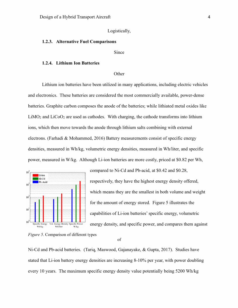
power, measured in W/kg. Although Li-ion batteries are more costly, priced at $0.82 per Wh,
compared to Ni-Cd and Pb-acid, at $0.42 and $0.28,
respectively, they have the highest energy density offered,
which means they are the smallest in both volume and weight
for the amount of energy stored. Figure 5 illustrates the
capabilities of Li-ion batteries’ specific energy, volumetric
energy density, and specific power, and compares them against
Figure 5. Comparison of different types of
Ni-Cd and Pb-acid batteries. (Tariq, Maswood, Gajanayake, & Gupta, 2017). Studies have
stated that Li-ion battery energy densities are increasing 8-10% per year, with power doubling
every 10 years. The maximum specific energy density value potentially being 5200 Wh/kg

Design of a Hybrid Transport Aircraft 5
(Ullman). Figure 6 illustrates a summary of efficiency, discharge time, operating temperature,
and lifespan of Li-ion batteries compared to other energy storage technologies.
Lithium ion batteries are 95-99% efficient. They have lifespans of 5-20 years with long
discharge times and a wide range of temperatures in which they can operate. Seal level
temperatures are usually around 15ºC and flight temperatures range from -44 ºC to -56 ºC at
cruise altitude. Considerations could be made to protect the batteries in the cool atmosphere. The
long discharge time makes these batteries ideal for transportation applications. High energy
storage batteries with long discharge time lead to maximum system efficiency combined with
minimal cost, weight, and volume. (Farhadi & Mohammed, 2016) With cost, weight, and
volume being critical factors in aircraft design, lithium ion batteries demonstrate good promise
statistically and have illustrated their capabilities through their use in small aircraft.
Figure 6. Performance Comparison of Li-ion Batteries
Batteries
A
With the increased level of technology for batteries, designing and building light and
general aviation aircraft is becoming a reality. Although initially costly in production, these
aircraft will not rely on fuel and will therefore have immense savings in the future. Prices will
also dwindle with increasing availability of technology and scale economy effects. Table 1 lists
electric aircraft that have flown as of 2016. (Riboldi & Gualdoni, 2016) These aircraft were
referenced to perform an electric aircraft sizing for a light or general aviation aircraft.
Table 1. Preliminary database of Electric Aircraft

Design of a Hybrid Transport Aircraft 6
1.3.
To perform the sizing of the battery of a small airplane designed for cross country flying
or training, the weight was first considered. For an electric aircraft, the weight is a combination
of the weight of the payload, batteries, electric motor, and the empty weight of the vehicle itself,
a
s
i
l
l
u
s
t
r
a
t
e
d
i
n
R
𝑊YX = 𝑊6 +𝑊5$ +𝑊R4Y + 𝑊E (1)
The mission profile consisted of the usual phases of take-off, climb, cruise, loiter, and
land. Typical flight sizing, relies on fuel fractions to define the fuel necessary for each portion
of the flight. (Roskam, Airplane Design Part 1: Preliminary Sizing of Airplanes, 2017) Since the
fuel would not change, and the weight would stay constant, this method of sizing would not be
appropriate. Instead, a relationship between the weights and the mission requirements was
examined. In electric aircraft, the most significant phases that affect the power are climbing,
cruising, and loitering. The power required for climb can be calculated through Eq. 𝑃𝑟𝑐𝑙𝑖𝑚𝑏=
𝑊YX𝑅𝐶 +tN𝜌B$"ER𝑉B$"ERu𝑆𝐶wB$"ER (2) relating air density during the
climb, constant airspeed, wing reference surface, the value of the drag coefficient, and the rate of
climb.
𝑃TB$"ER = 𝑊YX𝑅𝐶 +tN𝜌B$"ER𝑉B$"ERu𝑆𝐶wB$"ER (2)
Using
Error! Reference source not found.)
where

Design of a Hybrid Transport Aircraft 7
Error! Reference source not found.)
and the Oswald coefficient, e. With clean values of K and CD, the lift coefficient can be
calculated using 𝐶𝐿=2𝑊𝑡𝑜𝜌𝑉2𝑆 (3).
𝐶z =N{|G}~��
(3)
The next factor for sizing is the energy required. This involves energy required to climb,
cruise, loiter, and land. To estimate the energy required to climb, the time to climb and the
power required for the climb are taken into consideration, where the time to climb is defined in
𝑇𝑇𝐶=ℎ𝑐𝑟𝑢𝑖𝑠𝑒�𝑅𝐶� (4)
𝑇𝑇𝐶 = @����HJ
�� (4)
and the energy required for climb is defined in the following equation. (Riboldi & Gualdoni,
2016)
𝐸B$"ER = 𝑃TB$"ER𝑇𝑇𝐶 (5)
The energy required for cruise and loiter can be assumed to be the same. Different values
will be calculated because the densities, velocities, and drag coefficients differ for the phases.
(Riboldi & Gualdoni, 2016)
𝑃T =tN𝜌𝑉u𝑆𝐶w (6)
From there, the energy required for each phase can be calculated using
E-�*�. = P�-�*�.T-�*�. (7)
where the time of each phase relies on the range of the phase and the cruise speed at that phase.
(Riboldi & Gualdoni, 2016) Finally, the battery weight can be determined. With this
calculation, the propulsive efficiency is assumed to be less than 100%, providing the batteries

Design of a Hybrid Transport Aircraft 8
and motor with a higher requirement. The mission profile battery weight can be calculated using
the following equation. (Riboldi & Gualdoni, 2016)
𝑊R4Y,�� =7�F𝑚𝑎𝑥 ��
�^��]������HJ��^G�|J�
6, E4L���
�^��],������HJ,��^G�|J��5
� (8)
This sizing examination is limited in that it applies to current technology and small
aircraft. Sizing aircraft in other weight categories could prove to be more challenging,
especially with relying on current battery technology. A solution to transferring this process to a
larger aircraft, and utilizing current technology, could be to size a hybrid aircraft that could rely
both on the reusable power of batteries and on fuel to compensate for the additional size and
weight strain.
Hybrid aircraft are defined as aircraft where the propulsion is powered by more than one
type of energy source (Thauvin, et al., 2016). Different fuel sources provide the ability to
improve the aircraft’s performance, reduce fossil fuel reliance, reduce noise levels, and emit
fewer pollutants. Forms of Electrical Energy Storage (EES) would benefit hybrid vehicles in
their ability to store and use electric power, as needed.
Research was performed on an aircraft with twin-turbo propeller engines with 3500
thermal horsepower per engine, with the capabilities of traveling 400 nautical miles, at a ceiling
of 20,000 ft. The aircraft was also designed using technology for 2035, which would provide
batteries with higher energy densities (Thauvin, et al., 2016). This aircraft’s mission overview
can be viewed in Table 2. Its mission profile with the comparison of down-sized gas powered
turbine and standard conditions can be viewed in
Figure 7. Mission Profile Comparison of Sample Aircraft. The mission profile illustrates
the capabilities of added power provided by an energy storage unit combined with a reduced
engine. Also visible in the mission profile is added power sent to the storage unit during descent.

Design of a Hybrid Transport Aircraft 9
Energy recovering through the use of EES can be achieved through a few different
mechanisms. The research on this specific aircraft and the energy recovery examined the energy
gained through braking and through gravitational potential energy. The amount of energy
recovered and stored through braking is fairly minimal. For the research aircraft, the equivalent
amount of fuel saved is 2 kg, which is less than the amoung of fuel needed to taxi. These results
stemmed from assuming a gas turbine efficiency of 40%, and the braking system consisting of
disc brakes, thrust reversers, and airbrakes. (Thauvin, et al., 2016) Producing the equivalent of 2
kg of fuel or 0.19% of total energy used during this mission seems insubstantial.
Table 2. Mission Overview of Sample Aircraft
Figure 7. Mission Profile Comparison of Sample Aircraft
Utilizing gravitational potential energy during descent by windmilling propellers
produces energy that can be stored in the EES. On the experimental aircraft, four different
propeller modes were tested: folded, feathered, transparency, and wind turbine. Folded propeller
blades ideally produce zero drag during descent. Feathered blades rotate parallel to the direction
of the airflow. These add to the drag of the aircraft. Transparency blades result in rotating
propellers that don’t generate thrust or drag. Wind turbine blades add drag and energy to the
EES. Results from these trade studies demonstrated that propellers should be folded during
descent, and with a hybrid power generation system, transparency mode is most beneficial
during normal operations. (Thauvin, et al., 2016)

Design of a Hybrid Transport Aircraft 10
Other results regarding power efficiency provided additional improvements in operation.
The propeller efficiency could be increased by 49% if a hybrid electric system is utilized during
taxi, removing the minimum speed constraint. Energy during taxi could be decreased by 90% if
the taxi and descent phase could operate on purely electric power. Another consideration coud
be to use a single larger engine that has two times the power. This improves efficiency by
10.5%, but removes redundancies in the event of engine failure. Finally, the engine could be
sized to perform the climbing phase, with that phase being the most energy demanding.
(Thauvin, et al., 2016) Each of these considerations could be used to analyze and design future
aircraft of various sizes and explore the balance of the two power sources.
Other considerations for different types of batteries that could prove more energy dense
in future years have also been studied. Lithium ion batteries currently have a mass specific
energy content of Wh/kg, with a potential of 250 Wh/kg. Other variations of lithium batteries
could produce higher specific energies. Research is being conducted on Lithium-Sulfur (Li-S)
and Lithium-Oxygen (Li-O) batteries. Additionally, Zinc-Air (Zn-air) also have higher
theoretical specific densities. Their specific densities are summarized in Table 3, and an
illustration of their performance is present in
Figure 8. (Hepperle) These batteries could potentially provide an AV-gas fuel equivalent of
3800 Wh/kg, and power an electric aircraft. However, current technology is still limited. Hence,

Design of a Hybrid Transport Aircraft 11
the hybrid aircraft could provide an alternative aircraft which combines current battery
technology with reduced fuel and emissions.
Table 3. Summary of Theoretical Specific Energy
Figure 8. Current and expected battery technology
1.4. Project Objective
The purpose and objective of this project is to design a hybrid powered aircraft with the
following mission specifications. The payload will consist of a FAA maximum of 124
passengers and 2 crew members along with their luggage. The aircraft will have a maximum
range of 1720 nautical miles at maximum payload and a cruise speed of 500 kts. The required
takeoff field length will be 5,500 ft, and the required landing distance is 3,960 ft. The maximum
cruise altitude will be 40,000 ft. With the use of alternative power, provided by both Lithium ion
batteries and fuel, the project will focus on design trade-offs to power the short-range, narrow-
body aircraft that will reduce fuel usage, and provide a cheaper, cleaner, more energy-efficient
hybrid commercial vehicle.

Design of a Hybrid Transport Aircraft 12
1.5. Mission Specifications
1.5.1. Mission Specifications
The following consist of mission requirements for the HTA:
• Payload capacity: All Economy with 96 at 6 abreast; FAA limit: 124
• Number of crew members required: 2 pilots, 2 cabin attendants
• Range: 1720 nm
• Cruise speed and Mach number: 500 kts (M=0.75)
• Cruise altitutde: 40,000 ft
• Take-off field length: 5,500 ft
• Landing field length: 3,960 ft
• Approach speed: 128 knots
• Noise requirements: ≤97.5 EPNdb
1.5.2. Mission Profile
Figure 9. Mission Profile

Design of a Hybrid Transport Aircraft 13
1.6. Methodology
This hybrid aircraft will be designed and sized through a combination of
techniques that will account for both the fuel and batteries. Initially, Roskam’s approach using
an estimated take-off weight and fuel fractions will be used to address the changing fuel weight
during the various phases of the flight. The battery weight will be constant and will be sized
using the work of Riboldi and Gualdoni. Trade studies will be performed to assess the best usage
of fuel and batteries during each flight phase.
Once the weight has been sized, performance sizing and verification will be performed,
using the smallest size engine with the lowest weight. Then the design of the fuselage will take
place. This will be based on the 737-100 series aircraft, but modifications may be made to suit
the payload and change in power supply. From there, the wing will be sized. Again, this will be
based on the 737-100 aircraft, but changes may be made if parametric studies support changes in
sweep angle, wing thickness, or taper ratio. High lift systems will be applied if they are
beneficial. Analysis on the empinage design will be similar to the analysis of the wing. The last
feature of the aircraft to design will be the landing gear that promotes stability and control and
maintains the appropriate weight.
Drag analysis will additionally be performed to estimate the drag of the entire aircraft and
calculate a L:D ratio. If the aircraft, after all additions and design changes, is within 0.5% of its
initial weight, small changes will be made to reduce or resize. However, if the weight is not
within 0.5%, the aircraft sizing will need to be iterated until it is within 0.5% of the initial
weight.
1.7. Comparative Study of Airplanes with Similar Mission Performance
1.7.1. Comparison of Weights, Performance, and Geometries of Similar Airplanes
Table 4. Comparison of Aircraft Weights

Design of a Hybrid Transport Aircraft 14
Boeing 737-100
Boeing 737-200
Airbus A320NEO
Embraer ERJ-170-100
ARJ21-700STD
Bombardier CRJ200- ER
SUGAR Volt 765-096-RevA
Max Design Takeoff Weight (lbs)
97,000 100,000 174,165 79,344 89,287 51,000 150,000
Max Design Landing Weight (lbs)
89,700 95,000 146,165 72,311 83,037 47,000 143,300
Max Design Zero Fuel Weight (lbs)
81,700 85,000 138,450 66,447 77,062 44,000 135,300
Operating Empty Weight (lbs)
58,600 59,900 92,814 48,733 55,016 30,500 88,800
Max Structural Payload (lbs)
23,100 25,100 44,974 19,918 19,698 13,500 30,800
Seating Capacity 96 (FAA: 124)
(2 class)
124 (FAA:136)
(2 class)
150 (FAA: 180)
(2 class)
70 (single
class)
90 50 154
Usable Fuel (gallons)
3,540 3,460 6,268 3,071 3,417 2,052 2,196
Max Fuel Capacity (gallons)
4,720 4,780 6289.6 3,093 3,196 2,135 5,416
Source(s) (Boeing Commercial Airplanes, 2013)
(Boeing Commercial Airplanes, 2013)
(Airbus Commerial Aircraft, n.d.)
(Jane's All the World's Aircraft, 2013)
(Jane's All the World's Aircraft, 2013)
(Jane's All the World's Aircraft, 2013)
(Bradley & Droney, Subsonic Ultra Green Aircraft Research: Phase II- Volume II- Hybrid Electric Design Exploration, 2015)
Table 5.Comparison of Aircraft Performance (Assuming standard conditions at sea level)
Boeing 737-100
Boeing 737-200
Airbus A320NEO
Embraer ERJ-170-100
ARJ21-700STD
CRJ200-ER SUGAR Volt 765-096-RevA
Max Cruise Speed (Mach number)
0.82 0.82 0.82 0.82 0.82 0.85 0.7
Cruise Speed (mph)
580 580 598 529 518 534 537
Takeoff Field Length (MTOW) (ft)
5,499 5,499 6,857 4,866 5,578 5,800 8,180
Landing Field Length (ft)
3,960 3,960 5,020 4,029 5,086 4,850 --------
Service Ceiling (ft)
35,000 37,000 19,500 41,000 20,340 41,000 ---------

Design of a Hybrid Transport Aircraft 15
Cruising Altitude (ft)
23,500 23,500 37,000 41,000 35,000 37,000 42,000
Range (nm) 1,720 2,645 3,078 (3,700 with sharklets)
1,800 1,200 1,893 3,500
Source(s) (Boeing Commercial Airplanes, 2013)
(Boeing Commercial Airplanes, 2013)
(Airbus Commerial Aircraft, n.d.) (Jane's All the World's Aircraft, 2013)
(Jane's All the World's Aircraft, 2013)
(Jane's All the World's Aircraft, 2013)
(Jane's All the World's Aircraft, 2013)
(Bradley & Droney, Subsonic Ultra Green Aircraft Research: Phase II- Volume II- Hybrid Electric Design Exploration, 2015) (Bradley & Droney, Subsonic Ultra Green Aircraft Research: Phase I Final Report, 2011)
Table 6. Comparison of Aircraft Geometries
Boeing 737-100
Boeing 737-200
Airbus A320NEO
Embraer ERJ-170-100
ARJ21-700STD
CRJ200-ER SUGAR Volt 765-096-RevA
Overall length (ft)
94 ft 100 ft 2 in 123 ft 3.25 in 98 ft 1.25 in 109 ft 9.5 in 87 ft 10 in 139.7
Height (ft) (at max Woe)
37 ft 2 in 37 ft 3 in 38 ft 7 in 31 ft 11.25 in 27 ft 8.25 in 20 ft 5 in 35
Wing Area (ft2) 1098 1098 1317.5 782.8 859.6 587.1 1477.11 Wing span 93 ft 93 ft 117 ft 5.5
(including sharkets)
85 ft 3.5 in 89 ft 6.5 in 69 ft 7 in 169.3
Cabin width 12 ft 4 in 12 ft 4in 12 ft 1.75 in 8 ft 11.75 in 10 ft 3.75 in 8 ft 5 in ---------- Fuselage width 12 ft 4 in 12 ft 4 in 12 ft 11.5 in 9 ft 11 in 8 ft 10 in 148.7 Fuselage length 90 ft 7 in 96 ft 11 in 123 ft 3 in 98 ft 1 in 99 ft 10 in 80 ft 124.8 Total Bulk Cargo (ft3)
650 875 403 515 711.4 318 ----------
Source(s) (Boeing Commercial Airplanes, 2013)
(Boeing Commercial Airplanes, 2013)
(Airbus Commerial Aircraft, n.d.) (Jane's All the World's Aircraft, 2013)
(Jane's All the World's Aircraft, 2013)
(Jane's All the World's Aircraft, 2013)
(Jane's All the World's Aircraft, 2013)
(Bradley & Droney, Subsonic Ultra Green Aircraft Research: Phase II- Volume II- Hybrid Electric Design Exploration, 2015)

Design of a Hybrid Transport Aircraft 16
1.7.2. Configuration Comparison of Similar Airplanes
Figure 10. Boeing 737-100 aircraft configurations (Boeing Commercial Airplanes, 2013)

Design of a Hybrid Transport Aircraft 17
Figure 11. Boeing 737-200 aircraft configuration. (Boeing Commercial Airplanes, 2013)

Design of a Hybrid Transport Aircraft 18
Figure 12. Airbus A320NEO aircraft configuration (Airbus Commerial Aircraft, n.d.)

Design of a Hybrid Transport Aircraft 19
Figure 13. Embraer ERJ-170-100 aircraft configuration (Jane's All the World's Aircraft, 2013)

Design of a Hybrid Transport Aircraft 20
Figure 14. CRJ200-ER aircraft configuration (Canadair Regional Jet, 2016)

Design of a Hybrid Transport Aircraft 21
Figure 15. SUGAR Volt 765-096 RevA aircraft configuration (Bradley & Droney, Subsonic
Ultra Green Aircraft Research: Phase II- Volume II- Hybrid Electric Design Exploration, 2015)
1.8. Discussion
The configuration designs of the 737-100, 737-200, A320NEO, ERJ-170-100, CRJ200-
ER, and SUGAR Volt 765-096 RevA demonstrate common characteristics of transport aircraft,
as observed by Figure 10. Boeing 737-100 aircraft configurations Figure 15. SUGAR Volt 765-
096 RevA aircraft configuration Aircraft configurations allow for many architectural options.
Among these options are the wing sweep, wing style, wing position, propulsion system
integration, and other added aerodynamic features. Each of these features contributes to the
aircraft’s ideal design for performance, design for handling qualities, and meeting FAA
requirements on safety, ability, and noise.

Design of a Hybrid Transport Aircraft 22
The aircraft configurations display wings that have been aft swept. The sweep angle
depends on the speed of the aircraft. Subsonic speeds allow for small sweep angles. Transonic
speeds delay increase in drag, due to higher Mach numbers, by sweeping the wings 30 º -35º.
Supersonic aircraft have sweep angles of 45º -70º. (Mason, 2006) The sampled aircraft have
small sweep angles, with the Boeing 737-100 having a sweep angle of 25 º and the SUGAR Volt
765-096 RevA having sweep angle of 12.52º. (Bradley & Droney, Subsonic Ultra Green
Aircraft Research: Phase II- Volume II- Hybrid Electric Design Exploration, 2015)
Each of the aircraft also features a low wing, excluding the SUGAR Volt 765-096 RevA.
This typically provides efficient use of the fuselage cargo space and easy retraction of landing
gear. This characteristic also allows for better maneuverability and smooth landing. The
SUGAR Volt aircraft had additional systems to integrate involving batteries, which changed the
wing configuration. It features a high wing Truss Braced Wing (TBW), which is predicted to
save fuel consumption by 5-10% compared with conventional low wings. (NASA, 2014)
For the propulsion integration, the 737-100, 737-200, A320NEO, and ERJ-170-100 have
two pod mounted engines suspended below the wings. This meets civil aircraft requirements of
having more than one engine in the event that one becomes inoperable. The airplane must be
able to complete take-off in the event of one engine failure or only 50% power with 2 engines.
(Obert, 2009) The CRJ200-ER has two pod mounted engines fitted to the rear of the fuselage.
These two locations, below the wings and on the aft of the fuselage, are common configurations
for jet transport engines. Boeing has demonstrated that suspended engines don’t incur a drag
penalty. (Obert, 2009) This structural design of placing engines in nacelles suspended below the
wings has several advantages. Among these are load relief, with the engines opposing the lift
force; easy engine access for maintenance and repairs; and safety since the engines are further

Design of a Hybrid Transport Aircraft 23
from the passengers. (Obert, 2009) The SUGAR Volt 765-096 RevA has two engines suspended
below the wings along with two battery pods suspended below the wings. This configuration
allows for easy charge or exchange of batteries for quick transitions between flights.
Additionally, it balances the load of the battery pod weight. (Bradley & Droney, Subsonic Ultra
Green Aircraft Research: Phase II- Volume II- Hybrid Electric Design Exploration, 2015)
The tail and fin configurations also differ for the CRJ200-ER and SUGAR Volt 765-096
RevA aircraft compared to the 737-100, 737-200, A230NEO, and ERJ-170-100. The CRJ200-
ER and SUGAR Volt 765-096 RevA feature a T-tail; while the other aircraft feature fuselage
mounted conventional tails. Along with the fuselage mounted tails, the aircraft also have tail
plane mounted fins. These different configurations provide different aircraft control. A T-tail,
which is an empennage configuration where the tailplane is attached to the top of the fin,
typically accompanies fuselage mounted engines. With a T-tail arrangement, there is a risk for
the horizontal tail becoming engrossed by the wake of the wing at high angles of attack. (Mason,
2006) This is likely why the more common configuration is the conventional fuselage mounted
tail.
The Airbus A320NEO also has added sharklets to their wings. The Sharklet wingtip
devices are 7.9 feet wingtips that are standard on all NEO aircraft. They reduce fuel burn by
approximately 4%, and reduce annual CO2 emissions by approximately 9,000 tons per aircraft.
(Airbus Commerial Aircraft, n.d.) This added feature could be added to other A320 aircraft as
well as other aircraft models.
In summary, choosing various configurations can improve safety, increase performance,
and, with added features, reduce fuel consumption. The four common aircraft configurations
illustrate that the low swept wing, with two pod mounted engines suspended from the wing and

Design of a Hybrid Transport Aircraft 24
tail plane mounted fins meets the requirements of short to mid-range flights by providing greater
structural efficiency, less weight, and satisfactory stall characteristics. New advances in design
also demonstrate the benefits of the high wing TBW, as well as integration of batteries for hybrid
and electric vehicles.
2. Configuration Selection
2.1. Overall Configuration
The HTA will have a conventional configuration due to the expansive database of
conventional aircraft and design modeled after the Boeing 737 aircraft. From here, the
configurations of the fuselage, engine, wing, empennage, and landing gear will be presented with
short discussions on the rationale for selections.
2.1.1. Fuselage Configuration
The conventional fuselage will be designed to hold two cockpit crew members, 96
passengers at 6 abreast, and 2 flight attendants. Since it is designed for a short to medium range
flight, an approximate value of 175 lbs per person and 30 lbs of luggage per person will be
chosen for both the crew and the passengers. This totals 20,500 lbs, with 3,000 lbs being
designated for cargo. This cargo will be stored below the cabin floor in cargo containers that
have a capacity of 80 ft3. According to Roskam, typical luggage density is 12.5 lb/ft3 (Roskam,
Airplane Design Part 1: Preliminary Sizing of Airplanes, 2017). Therefore, 240 ft3 of baggage
volume will be required for bagge storage in 3 containers.
With 6 abreast seating, there will be 16 rows, which maintains a shorter fuselage.
Although 5 abreast seating may be more comfortable for passengers, this would add an
additional 4 rows of seating, which increases the fuselage length and the aircraft weight. The
seat pitch for tourist/economy/coach passengers ranges from 34-36 inches, and could be 30-32

Design of a Hybrid Transport Aircraft 25
inches for high density seating arrangements. (Roskam, Airplane Design Part 1: Preliminary
Sizing of Airplanes, 2017) The hybrid aircraft will have a 34 in. seat pitch, and 18 in. aisles to
provide a comfortable mode of transportation. Further design layouts of the fuselage will be
presented in the fuselage design section.
2.1.2. Engine Configuration
The hybrid aircraft will have two engines suspended below the wings. Two engines
provides for redundancy in the event of a single engine failure or 50% failure of both engines.
The engines will be stored in nacelles, and two battery pods will also be stored in nacelles
attached under the wing. Having the batteries outside of the aircraft allows for easier access
when charging and easier exchange of the batteries for quick transitions between flights. 737-
100 model airplanes used JT8D turbofan engines. For the hybrid airplane, the design could
include two hFan engines with 1,380 hp and thrust equivalent to 21,000 lbf of Boeing thrust.
Although buried engines produce less drag, having the engines stored in pods outside the
fuselage also provides the ability to easily repair or exchange as technology improves. This
configuration also provides optimal engine operation, in-flight wing bending relief, and engine
stability. Mounting the engines above the wings also has advantages, including less debris
ingestion and lower noise levels. However, this is not beneficial aerodynamically, and will not
be considered.
2.1.3. Wing Configuration
For the wing configuration, the airplane will have a low Cantilever wing. Low wings are
ideal for transport vehicles due to the increased safety of the aircraft, increased cargo volume,
and ease of maneuverability. High wings are generally best for short take-offs and landings, but
offer very little cargo space. Mid wings provide the least drag during flight due to their design,

Design of a Hybrid Transport Aircraft 26
with the wings being continuous with the fuselage. This design would not be ideal for the hybrid
transport due to the fact that the fuselage volume is reduced to accommodate the wings.
The wings will be swept aft with the characteristics of the wings, including sweep angle,
aspect ratio, thickness ratio, and other features, being discussed and explored in detail later.
2.1.4. Empennage Configuration
The empennage consists of the stabilizing tail and added features on the aircraft. The
configuration for the hybrid transport aircraft will be a single verticle tail mounted to the
fuselage. Mounting to the fuselage provides adequate support. Since the tails are designed to
help recover from stalling and spinning, the vertical configuration is more reliable than the T-tail
configuration, which may be affected by the air flow, potentially causing deep stall.
2.1.5. Landing Gear Configuration
Since the hybrid vehicle is a narrow-body vehicle, the bicycle landing gear can easily be
used. This does limit the takeoff and landing locations to level ground since the landing gear
will not be able to rotate. With retractable landing gear mounted on the fuselage, the drag during
flight will not be increased, and the gears are well-supported. Having the landing gear mounted
to the nose of the fuselage provides more stability than aft wheel mounted landing gear.
However, this position increases the weight. Since weight is such a large factor in the design,
due to the already heavy batteries, mounting the retractable landing gear to the aft of the wheel
would be beneficial.
The remaining aspects of the configuration, including number of main fear struts, number
of tires, and the retraction kinematics will be discussed in detail when the landing gear is sized.
In summary the overall configuration of the aircraft will be a conventional fuselage
designed to comfortably hold 96 passengers and their luggage, The aircraft will be supported by

Design of a Hybrid Transport Aircraft 27
conventional low wings with 2 engines mounted below the wings and 2 batteries mounted below
the wings. The vertical tail will provide the stability during flight, and the tricycle aft wheel
retractable landing gear will provide adequate support with minimal weight for landing.
3. Weight Sizing and Weight Sensitivities
Using data for takeoff weights and empty weights of similar aircraft, a plot of gross
takeoff weight vs. empty weight will be analyzed. The axes will be scaled logarithmically to
create a log-log plot of the weight data.. The regression coefficients will be calculated to
determine the weight required for takeoff and for the overall mission. A sensitivity study will be
performed using the AAA Program.
3.1 Data Base for Takeoff Weights and Empty Weights of Similar Airplanes
The following data in Table 7 provide takeoff weights and empty weights for comparison
to the HTA. Roskam additionally provides transport jet weights for comparison. The takeoff
weights and empty weights can be related linearly when graphing the log of the takeoff weight
and the log of the empty weight. The plot of this relationship is illustrated in Figure 16.
Table 7. Aircraft Takeoff and Empty Weights
Aircraft Takeoff Weight (lbs) Empty Weight (lbs) Source 765-093 FREE 182,600 94,400 (Bradley & Droney, Subsonic Ultra Green
Aircraft Research: Phase II- Volume II- Hybrid Electric Design Exploration, 2015)
765-095 SUGAR High 138,300 81,700 (Bradley & Droney, Subsonic Ultra Green Aircraft Research: Phase II- Volume II- Hybrid Electric Design Exploration, 2015)
Balanced 765-095 (1,380 Hp)
140,700 84,300 (Bradley & Droney, Subsonic Ultra Green Aircraft Research: Phase II- Volume II- Hybrid Electric Design Exploration, 2015)
Balanced 765-095 (1,750 Hp)
139,700 83,800 (Bradley & Droney, Subsonic Ultra Green Aircraft Research: Phase II- Volume II- Hybrid Electric Design Exploration, 2015)
Core Shutdown 765-095 (7,150 Hp)
190,000 102,600 (Bradley & Droney, Subsonic Ultra Green Aircraft Research: Phase II- Volume II- Hybrid Electric Design Exploration, 2015)
Boeing 737-100 97,000 58,600 (Boeing Commercial Airplanes, 2013) Boeing 737-200 100,000 59,900 (Boeing Commercial Airplanes, 2013) Airbus A320NEO 174,165 92,814 (Jane's All the World's Aircraft, 2013) Embraer ERJ-170-100 79,344 48,733 (Jane's All the World's Aircraft, 2013) ARJ21-700STD 89,287 55,016 (Jane's All the World's Aircraft, 2013) CRJ200- ER 51,000 30,500 (Jane's All the World's Aircraft, 2013)

Design of a Hybrid Transport Aircraft 28
SUGAR Volt 765-096 RevA
150,000 88,800 (Bradley & Droney, Subsonic Ultra Green Aircraft Research: Phase II- Volume II- Hybrid Electric Design Exploration, 2015)
Figure 16. Log-Log Plot of Takeoff Weight vs. Empty Weight with included trendline and linear regression equation
From the plot, the regression line constants A and B can be determined, since the log of
the weights has the following relationship:
log(Wto)= A+B*log(We) (9)
Thus, A=0.1776 and B= 0.9195, as demonstrated by the regression equation in the plot. In Part 1
of Roskam’s Airplane Design Volumes, Roskam lists the regression line constants for various
airplane types. These are included in Figure 17. The B values obtained in this analysis are
similar, with B having an 11.44% margin of error. However, the A values are very different.
This could be due to the type of aircraft in the database. 5 of the 12 aircraft included are hybrid
vehicles. The remaining 7 are conventional fuel-powered aircraft. The A value for this database
differs by -113.2%, with the transport jet A coefficient calculated as 0.0833 and the B value as
1.0383.
The other factor that could impact the weights could be the materials used for the primary
and secondary structures, which would affect the takeoff weight and empty weight. Roskam’s
database consists of Boeing 727, 737, 747, 757 and 767 aircraft, McDonnell Douglas DC 8, 9,
and 10 aircraft, Airbus A300 and A310 aircraft, and several others. The Boeing aircraft were
constructed from aluminum alloy, aluminum, and graphite composites. (Jane's All the World's
y = 0.9195x + 0.1776
4.4
4.6
4.8
5
5.2
4.6 4.7 4.8 4.9 5 5.1 5.2 5.3 5.4
log(
we)
log(wto)
Log(Wto) vs. Log(We)

Design of a Hybrid Transport Aircraft 29
Aircraft, 2013) The Airbus aircraft were constructed from aluminum alloy, steel, and titanium.
The SUGAR aircraft have incorporated metal-matrix composites, ceramics, high temperature
polymer composites, thermoplastic composites, carbon, and nanocomposites. These will lighten
the weight of the structure, landing gear, and engine nacelles. (Bradley, Droney, & Allen, 2015)
Figure 17. Regression Line Constants for Aircraft
For future calculations, both Roskam’s constants and the calculated constants will
initially be used and comparisons in results will be made before determining the constant that
will be used in the end.
3.2. Determination of Mission Weights
The following mission weights will be estimated: 𝑊5$,𝑊YX,𝑊=,𝑊6, and𝑊R4Yusing
comparisons to similar aircraft, calculations from Roskam and Riboldi, and iterating through the
AAA program to verify and refine estimations.
Takeoff weight, Wto, consists of the sum of the operating empty weight of the aircraft,
Woe, with the weight of the fuel, Wf, weight of the payload, Wpl and the added weight of the
b
a
t

Design of a Hybrid Transport Aircraft 30
𝑊𝑡𝑜=𝑊𝑜𝑒+𝑊𝑓+𝑊𝑝𝑙+𝑊𝑏𝑎𝑡 (10).
𝑊YX = 𝑊X6 +𝑊= +𝑊5$ +𝑊R4Y (10)
Note that the operating empty weight consists of the sum of the empty weight, weight of the
trapped fuel and oil, and the weight of the crew, as summarized in 𝑊𝑜𝑒= 𝑊6 +𝑊Y=X +
𝑊BT6[(11)
𝑊X6 = 𝑊6 +𝑊Y=X +𝑊BT6[ (11)
For 𝑊𝑡𝑜= 𝑊X6 +𝑊= +𝑊5$ + 𝑊R4Y (10), the weights of
each of the parts will need to be calculated. Although the payload weight is known, the
remaining values will need to be calculated. The process for this will be conducted as follows.
Initially, a takeoff weight will be estimated using data from similar aircraft. From there, the
weights of the fuel, and batteries will be calculated. Roskam’s fuel fraction method will be used
to calculate the mission fuel weight; while Riboldi’s battery sizing method will be employed to
estimate mission battery weight. Then, the operating empty weight will be calculated to find an
allowable value of the empty weight. AAA will be used to iterate and find an empty weight
within 0.5% of the tentative empty weight.
3.3. Manual Calculation of Mission Weights
3.3.1. Payload Weight
The payload weight consists of the passengers and their luggage. Based on the desired
configuration of the cabin, 96 passengers will be assumed to weigh 175 lbs each and carry 30 lbs
of luggage. Thus the total payload weight is 19,680 lbs.
3.3.2. Estimated Takeoff Weight Method 1
To estimate the takeoff weight, there are two methods. The first consists of examining a
database of aircraft and comparing Wto to Wpl. The database, displayed in Table 8, consists of
turbojet transport aircraft and conceptual hybrid aircraft. Using the data, an average ratio of Wpl

Design of a Hybrid Transport Aircraft 31
to Wto was calculated as 0.237. Since the payload weight is a known value, the takeoff weight
can be estimated using the ratio. Using a 96 passenger payload yields a takeoff weight value of
83,006.38 lbs. If the payload is increased to hold 100 passengers, the takeoff weight increases to
86,464.98 lbs. Finally, if the payload is increased to 108 passengers, the takeoff weight estimate
is 93,382.18 lbs.
Table 8. Data for Wto Comparison
737-100 737-200 A320NEO ERJ-170-
100 ARJ21-700STD
CRJ200- ER
SUGAR Volt 765-096-RevA 737-300
McDD DC9-80 A320
Wto 97,000 100,000 174,165 79,344 89,287 51,000 150,000 135,000 140,000 145,000 Wpl 23,100 25,100 44,974 19,918 19,698 13,500 30,800 35,000 38,000 42,000
The second method to calculate takeoff weight involves knowledge of more values.
Therefore, it will be discussed later. With an estimation of takeoff weight from the database,
calculating the fuel weight will be the next step.
3.3.3. Determination of Mission Fuel Weight
To determine the mission fuel weight, Wf, the weight of the fuel used during the mission
and the weight of the reserve fuel will need to be known. To calculate the weight of the fuel for
the mission, Roskam’s fuel fraction method will be employed. This consists of breaking down
the mission into phases and estimating the fuel for each phase. The phases for the mission are:
Phase 1: Engine start and warm-up, Phase 2: Taxi, Phase 3: Takeoff, Phase 4: Climb, Phase 5
Cruise, Phase 6: Loiter, Phase 7: Descent, and Phase 8: Land, taxi, and shut-down. This process
will be presented for the 96 passenger payload and considered for a fuel powered flight. From
there, fuel can be reduced by using batteries to power various phases of flight and eliminating
parts of the fuell fraction process. AAA will then be used to calculate weights for the aircraft if it
had used all fuel, to compare, as well as using fuel for stages 1-4 vs. fuel for stages 1-3, and 5.

Design of a Hybrid Transport Aircraft 32
To calculate the mission fuel weight, the sum of the fuel used and the fuel in reserves will
need to be known.
𝑊= = 𝑊=>963 +𝑊=T69 (12)
W¡¢�.£ is the fuel used during the mission; while W¡�.� is the fuel reserves required for the
mission.These reserves are specified by FAR regulations. For a fully fuel-powered aircraft, the
reserves will be 25% of the fuel used. The reserve quanitities will change depending on the fuel
used during different mission phases. The fuel used will be calculated using the fuel fraction
method. Each phase will have an estimated or calculated fuel fraction, which is the ratio of the
ending weight of the phase to the beginning weight of the phase.
Table 9. Suggested Fuel-Fractions for Mission Phases
As seen in
Table 9, the fuel fractions for phases 1, 2, 3, 4, 7, and 8, have been estimated and published by
Roskam. (Roskam, Airplane Design Part 1: Preliminary Sizing of Airplanes, 2017) These
values for transport jets will be used in the calculation of the fuel-powered aircraft. The phase 1
fuel fraction of 0.990 is the ratio of 𝑊t/𝑊YX . The phase 2 fuel fraction of 0.990 is the ratio of

Design of a Hybrid Transport Aircraft 33
𝑊N/𝑊t. 0.995 is the ratio of 𝑊u/𝑊N, which is the phase 3 fuel fraction. 0.980 is the ratio of
𝑊¤/𝑊u; 0.990 is the ratio of 𝑊¥/𝑊¦, and 0.992 is the ratio of 𝑊¦/𝑊§. The fuel fractions,
𝑊 /𝑊¤ and 𝑊©/𝑊 , for phases 5 and 6, respectively, will be calculated.
F
o
r
a
j
e
t
a
i
r
p
l
a
n
e
,
B
r
e
𝑅BT = ª~BC«BT¬zwBT𝑙𝑛 ¬{®
{̄ (13)
The velocity for cruise is known, along with the range. The lift to drag ratio and specific fuel
consumption values can be found in Roskam’s part 1. For transport jets in cruise, L/D ranges
from 15-24s and c± ranges from 0.5-0.9. The following values will be used to estimate 𝑊 /𝑊¤:
𝑉 = 500𝑘𝑡𝑠, 𝑐µ = 0.5, zw= 22, 𝑎𝑛𝑑𝑅BT = 1656𝑛𝑚. This yields 𝑊 /𝑊¤ = 0.928.
For the loiter phase, Breguet’s endurance equation, equation 𝐸𝑙𝑡𝑟= ª tBC^|�
« ¬zw$YT𝑙𝑛 ¬{̄
{½
(14) below, for jet airplanes can be used (Roskam, Airplane Design Part 1: Preliminary Sizing of
Airplanes, 2017).
𝐸$YT = ª tBC^|�
« ¬zw$YT𝑙𝑛 ¬{̄
{½ (14)
E)1� is the loiter time in hours. According to Roskam, 𝑐µ$YT ranges from 0.4-0.6, and L/D for the
loiter phase ranges from 14-18. Using E)1� = 0.75ℎ𝑜𝑢𝑟𝑠, 𝑐µ$TY = 0.4, 𝑎𝑛𝑑 zw= 18,
𝑊 /𝑊© =0.981.
Now that the fuel fractions for each phase are known, the mission fuel fraction, 𝑀==, can
be calculated using 𝑀𝑓𝑓= ¬{Á{|G∏ {�ÃÁ
{�¥
"Ät (15) (Roskam,
Airplane Design Part 1: Preliminary Sizing of Airplanes, 2017).

Design of a Hybrid Transport Aircraft 34
𝑀== = ¬{Á{|G∏ {�ÃÁ
{�¥
"Ät (15)
Therefore, 𝑀== = 0.99 ∙ 0.99 ∙ 0.995 ∙ 0.98 ∙ 0.928 ∙ 0.981 ∙ 0.99 ∙ 0.992 = 0.854. Using the
m
i
s
s
i
o
n
f
u
e
l
f
r
a
c
t
i
o
n
,
t
h
𝑊=�HJÆ = Ç1 − 𝑀==É𝑊YX (16)
F
r
o
m
e
q
u
a
t
i
o
n
R
E
F
_
R
e
3.3.4.
A
s
e
c
o
n
d
m
e
t
h
o
d
t
o
𝑙𝑜𝑔tË𝑊YX = 𝐴 + 𝐵 ∙ 𝑙𝑜𝑔tË(𝐶 ∙ 𝑊YX − 𝐷) (17)
Roskam’s A and B values will be used since the calculated B value will not yield a real
solution for the equation and hence not provide an estimated takeoff weight. D is the sum of the
crew and passenger weight along with their cargo. Assuming 96 passengers and 4 cabin and
c
r
e
w
m
e
m
b
e
𝐶 = �1 − (1 + 𝑀T69)Ç1 −𝑀==É − 𝑀Y=X� (18)
𝑀T69 is the reserve fuel fraction; 𝑀==is the mission fuel fraction; and 𝑀Y=X is the trapped fuel and
oil fraction. 𝑀Y=X is assumed to be 0.005, and Mres is assumed to be 0.25. (Roskam, Airplane
Design Part 1: Preliminary Sizing of Airplanes, 2017) 𝑀== varies based on the amount of fuel

Design of a Hybrid Transport Aircraft 35
required. This calculation will be reviewed in the following section. For 100% fuel use,
𝑀== =0.854. With fuel use during stages 1-4, 𝑀== =0.956. With fuel use during stages 1-3 and
5, 𝑀== =0.905. Three different values of C were calculated based on the three different fuel
options. Call fuel=0.813, C1-4=0.9396, and C1-3,5=0.876. These three different values provided
t
h
r
e
e
d
i
f
f
e
r
e
n
t
t
a
k
e
o
f
f
3.3.5. Determining Allowable Value for Empty Weight
To determine an allowable value for empty weight, for a fuel-powered aircraft, first a
tentative value for the operating empty weight is calculated, using the following equation:
𝑊X6Y6#Y = 𝑊YX7>699 −𝑊= −𝑊5$ (19)
Since the W1Ï/¢.��,W¡, andW-) are known, where W1Ï/¢.�� = 83,006.38lbs,W¡ =
15,111.6lbs, andW-) = 19,680𝑙𝑏𝑠, then WÏ.1.&1 = 48,214.8lbs. Then, a tentative value for
the empty weight is calculated, using the following equation
𝑊6|JI| = 𝑊X6|JI| −𝑊Y=X −𝑊BT6[ (20)
Since this is a tentative estimate, W1¡Ï will not be subtracted at this time. It can add as much as
0.5% of the takeoff weight, but can initially be neglected. (Roskam, Airplane Design Part 1:
Preliminary Sizing of Airplanes, 2017) With the weight of the crew and the tentative operating
empty weight, W.ÔÕÖÔ = 48,214.8 − 820 = 47,394.8lbs. This tentative weight is then

Design of a Hybrid Transport Aircraft 36
compared to a calculated weight. If these values are not within 0.5%, adjustments are made to
the takeoff weight guess and the process is iterated.
Figure 18 illustrates the trend of takeoff weights and empty weights for transport jets.
The regression line for the data has the following equation:
𝑊6 = 𝑖𝑛𝑣𝑙𝑜𝑔tË((𝑙𝑜𝑔tË𝑊YX − 𝐴)/𝐵)) (21)
Since A and B are known, along with the guessed takeoff weight, W. is calculated as 47,394.8
lbs. Since these two weights are close, but not within 0.5% of each other, adjustments will be
made to the takeoff weight guess and the empty weight will be recalculated. This process will be
completed using AAA.

Design of a Hybrid Transport Aircraft 37
Figure 18. Weight Trends for Transport Jets
3.3.6.
To determine mission battery weight, the method of Riboldi and Gualdoni will be used.
C
I
T
A
T
I
O
N

Design of a Hybrid Transport Aircraft 38
specific power and specific energy values are values for lithium ion batteries by the year 2025,
and will likely increase further with advancements in batteries. (Hepperle)
Since the climb, cruise, and loiter phases are the longest phases of the flight, the power
and energy required for these phases will be taken into account. To calculate the power and
e
n
e
r
g
y
f
o
r
t
h
e
s
e
p
h
a
s
e
s
From there, the power for each phase can be calculated, using S=1,341 ft2 and the
velocity at cruise to be 575 mph. The power at loiter is 405.34 watts, and the power at cruise is
736.42 watts. The energy required for loiter is 1,094,411.5 joules, and the energy required for
cruise is 8,779,440.79 joules.
U
s
i
n
g
e
q
u
a
t
i
o
n
R
3.4. AAA Calculation of Mission Weights
The following figures summarize the output parameters generated by AAA given the
input parameters of the mission. The summary of data in the first two figures is for a twin
turbojet engine fuel-powered aircraft. The manual calculations and AAA calculations proved to
be very similar for the fuel-powered aircraft, with the AAA output weights being lower. AAA
calculated the design point takeoff weight to be 71,947.6 lbs and the empty weight to be 39,775.9
lbs. The manual calculation produced an estimate of 77,602.6 lbs for the takeoff weight and
45,439.32 lbs for the empty weight. For an all fuel-aircraft, AAA calculated 11,554 lbs of fuel,

Design of a Hybrid Transport Aircraft 39
including 25% reserves; while manual calculations found 15,111.6 lbs of fuel necessary,
including the 25% reserve fuel.
Figure 19. AAA output with all fuel aircraft with 2 turbojet engines
Figure 20. We vs. Wto of 2 turbojet engine fuel-powered aircraft with ideal design point of Wto=71,635.9 lbs and We=39,775.9 lbs
Design of a Hybrid Transport Aircraft 40
3.5.Takeoff Weight Sensitivities
3.5.1. Manual Calculations of Takeoff Weight Sensitivities
Aircraft takeoff weight depends on many factors. These include the payload weight,
empty weight, range, endurance, lift to drag ratio, and specific fuel consumption. (Roskam,
Airplane Design Part 1: Preliminary Sizing of Airplanes, 2017) Sensitivity studies will be
performed on these to determine which parameters impact the design. Using Roskam’s
correlation coefficients of A=0.083 and B=1.038, the calculated C values, the combined crew
and passenger payload weight, D=20,500 lbs, and the force, F=250,337.6 lbs, sensitivities for the
takeoff weight to: payload, empty weight, range, endurance, cruise speed, L/D, and specific fuel
consumption will be calculated for the HTA. Additionally, the airplane growth factor due to
payload will be calculated. To illustrate the concept, calculations will be completed for the fuel-
powered aircraft, initially, with sensitivities also being calculated for various amounts of fuel use.
This includes using fuel in stages 1-4, 1-3 and 5, and sensitivities for an electric aircraft.
In order to calculate the sensitivities, the takeoff weight needs to be established. For the
purposes of these sensitivities, the takeoff weight used will be the manually calculated takeoff
weight of 77,602.6 lbs. Using equation log(Wto)= A+B*log(We)
(9) and taking the partial derivative of the takeoff weight with respect to the empty weight
produces:
Ø{|GØ{J
= 𝐵𝑊YX Ù𝑖𝑛𝑣𝑙𝑜𝑔¬$X7({|G)ÚÛ
ÜÝÚt (22)
Substituting the values gives: ÞßÔàÞßÕ
= (1.038)(77,602.6) Ù𝑖𝑛𝑣𝑙𝑜𝑔¬$X7(¥¥,©ËN.©)ÚË.˦ut.Ëu¦
ÝÚt
=1.89. As a
result, for a fuel-powered aircraft, the takeoff weight must be increased by 1.89 lbs for each
pound of increase in the empty weight. 1.89 is the growth factor due to empty weight for the
fuel-powered aircraft. If the aircraft used fuel during phases 1-4, the growth factor would be

Design of a Hybrid Transport Aircraft 41
1.866, and it would remain the same for fuel use in phases 1-3 and 5. If the aircraft were all
electric, the growth factor would be 2.22.
To compute the sensitivities of the takeoff weight to the payload weight, the partial
d
e
r
i
v
a
t
i
v
e
o
f
e
q
u
a
t
i
o
n
Ø{|GØ{F^
= 𝐵(𝑊YX){𝐷 − 𝐶(1 − 𝐵)𝑊YX}Út (23)
Substituting the remaining values produces ÞßÔàÞßãä
= 1.038(77,602.6){20,500 − 0.813(1 −
1.038)77,602.6}Út = 3.5. Therefore, if the payload increases by 1 lb, the takeoff weight increases
by 3.5 lbs for the fuel powered aircraft. When fuel is used in stages 1-4, the airplane growth
factor due to payload is 2.5; with fuel use in stages 1-3, and 5, it’s 3.5; and for an electric
airplane, the airplane growth factor due to payload is 2.2.
In order to calculate the sensitivity of takeoff weight to range, endurance, speed, specific
fuel consumption, and lift to drag ratio, a generic case will be considered. The variable 𝑦 will
represent any parameter, excluding payload. Thus, the following equation represents the takeoff
weight sensitivity to a parameter 𝑦:
Ø{|GØæ
= {𝐶𝑊YX(1 − 𝐵) − 𝐷)Út𝐵𝑊YXN ¬Ø�
Øæ (24)
Using Breguet’s equations and
𝐹 = −𝐵𝑊YXN {𝐶𝑊YX(1 − 𝐵) − 𝐷}Út(1 + 𝑀T69)𝑀== (25)
Breguet’s partials can be derived. They are available in Table 10, below. Using the manually
calculated values, F=250,337.6 lbs.
Table 10. Breguet Partials for Propeller and Jet Airplanes

Design of a Hybrid Transport Aircraft 42
Substituting in range and endurance for y, respectively, yields
Ø{|GØ�
= 𝐹𝑐µ ª𝑉 ¬zw«
Út= 16.7lbs/nm and Ø{|G
Ø�= 𝐹𝑐µ ¬
zwÚt= 7,699.7 lbs/hr. In summary, if the
range of the fuel aircraft is decreased by 1 nm, the takeoff weight decreases by 16.7 lbs. If the
endurance is increased by 1 hour, the takeoff weight is increased by 5,563 lbs.
Continuing to use Breguet’s partials in Table 10, the sensitivities of takeoff weight to
cruise speed will be calculated. Assuming a cruise speed of 500 kts or M=0.75, L/D=22, cruise
range of 1656 nm, and specific fuel consumption of 0.5, Ø{|GØ~
= −37.7 lbs/kt. Therefore, if the
cruise speed could be increased without changing any parameters, the gross takeoff weight
would decrease. Despite these results, this sensitivity result is not practical. An increase in
cruise speed results in a decrease in the lift coefficient and thus a decrease in the lift to drag ratio.
The specific fuel consumption will also change. (Roskam, Airplane Design Part 1: Preliminary
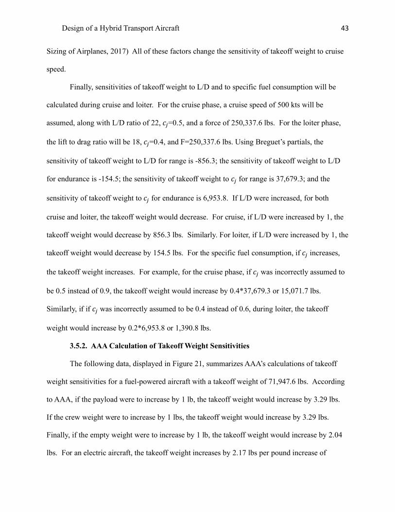
Design of a Hybrid Transport Aircraft 43
Sizing of Airplanes, 2017) All of these factors change the sensitivity of takeoff weight to cruise
speed.
Finally, sensitivities of takeoff weight to L/D and to specific fuel consumption will be
calculated during cruise and loiter. For the cruise phase, a cruise speed of 500 kts will be
assumed, along with L/D ratio of 22, 𝑐µ=0.5, and a force of 250,337.6 lbs. For the loiter phase,
the lift to drag ratio will be 18, 𝑐µ=0.4, and F=250,337.6 lbs. Using Breguet’s partials, the
sensitivity of takeoff weight to L/D for range is -856.3; the sensitivity of takeoff weight to L/D
for endurance is -154.5; the sensitivity of takeoff weight to 𝑐µ for range is 37,679.3; and the
sensitivity of takeoff weight to 𝑐µ for endurance is 6,953.8. If L/D were increased, for both
cruise and loiter, the takeoff weight would decrease. For cruise, if L/D were increased by 1, the
takeoff weight would decrease by 856.3 lbs. Similarly. For loiter, if L/D were increased by 1, the
takeoff weight would decrease by 154.5 lbs. For the specific fuel consumption, if 𝑐µ increases,
the takeoff weight increases. For example, for the cruise phase, if 𝑐µ was incorrectly assumed to
be 0.5 instead of 0.9, the takeoff weight would increase by 0.4*37,679.3 or 15,071.7 lbs.
Similarly, if if 𝑐µ was incorrectly assumed to be 0.4 instead of 0.6, during loiter, the takeoff
weight would increase by 0.2*6,953.8 or 1,390.8 lbs.
3.5.2. AAA Calculation of Takeoff Weight Sensitivities
The following data, displayed in Figure 21, summarizes AAA’s calculations of takeoff
weight sensitivities for a fuel-powered aircraft with a takeoff weight of 71,947.6 lbs. According
to AAA, if the payload were to increase by 1 lb, the takeoff weight would increase by 3.29 lbs.
If the crew weight were to increase by 1 lbs, the takeoff weight would increase by 3.29 lbs.
Finally, if the empty weight were to increase by 1 lb, the takeoff weight would increase by 2.04
lbs. For an electric aircraft, the takeoff weight increases by 2.17 lbs per pound increase of

Design of a Hybrid Transport Aircraft 44
payload. The takeoff weight increases by 2.17 lbs for every 1 pound increase in crew, and the if
the empty weight increases by 1 pound, the takeoff weight increases by 1.86 lbs.
The sensitivities for the hybrid aircraft with fuel use in phases 1-4 or 1-3 and 5 have
similar values with their values being between the fuel-powered aircraft and the electric aircraft.
This holds true for both the manual calculations and the AAA calculations.
Figure 21. Takeoff weight sensitivities calculated by AAA for fuel-powered aircraft
Figure 22. Takeoff weight sensitivities calculated by AAA for electric aircraft
3.6. Trade Studies
Trade studies of takeoff weight versus L/D, payload, range, and specific fuel
consumption will be performed. These trade studies are being performed on the HTA which will
use fuel in stages 1-4. Additionally, a trade study of range vs. payload will be performed by
AAA for the fuel-powered aircraft to compare.

Design of a Hybrid Transport Aircraft 45
3.7. Takeoff Weight vs. Critical Mission Parameters
3.7.1. Takeoff Weight vs. L/D
Figure 23. Takeoff Weight vs. L/D for Cruise
Figure 24. Takeoff Weight vs. L/D for Loiter
45500475004950051500535005550057500595006150063500
12 13 14 15 16 17 18 19 20 21 22 23 24 25 26
Wto
(lb
s)
L/D
Wto vs. L/Dcr
53200
53400
53600
53800
54000
54200
54400
54600
54800
13 14 15 16 17 18 19 20 21 22 23 24
Wto
(lb
s)
L/D
Wto vs. L/Dltr

Design of a Hybrid Transport Aircraft 46
3.7.2. Takeoff Weight vs. Payload
Figure 25. Takeoff Weight vs. Payload Weight (ranges from 80 passengers to 124 passengers)
3.7.3. Takeoff Weight vs. Range
Figure 26. Takeoff Weight vs. Range
53000
53200
53400
53600
53800
54000
54200
54400
16000 17000 18000 19000 20000 21000 22000 23000 24000 25000 26000
Wto
(lbs
)
Wpl (lbs)
Wto vs. Wpl
48000
50000
52000
54000
56000
58000
60000
62000
1480 1580 1680 1780 1880 1980 2080
Wto
(lbs)
Range (nm)
Wto vs. Range

Design of a Hybrid Transport Aircraft 47
3.7.4. Takeoff Weight vs. Specific Fuel Consumption
Figure 27. Takeoff Weight vs. Specific Fuel Consumption during Cruise
Figure 28. Takeoff Weight vs. Specific Fuel Consumption during Loiter
50,000.0052,000.0054,000.0056,000.0058,000.0060,000.0062,000.0064,000.0066,000.0068,000.0070,000.00
0.4 0.5 0.6 0.7 0.8 0.9 1
Wto
(lbs)
Cj (lbs/lbs/hr)
Wto vs. Cj cr
53,000.00
53,500.00
54,000.00
54,500.00
55,000.00
55,500.00
56,000.00
56,500.00
0.3 0.4 0.5 0.6 0.7 0.8 0.9
Wto
(lbs)
Cj (lbs/lbs/hr)
Wto vs. Cj ltr

Design of a Hybrid Transport Aircraft 48
Figure 29. Range vs. Payload
3.8. AAA Calculation of Range vs. Payload
Figure 30. Range vs. Payload with design point Wpl=19,630.6 lb and Rcr=1,638.7 nm for fuel-powered aircraft
3.9. Trade Study Conclusions
The estimated takeoff weight of 53,778.38 lbs, which is the sum of the manually
calculated takeoff weight for the HTA and the batteries, assuming fuel is used during phases 1-4
1690
1700
1710
1720
1730
1740
1750
1760
1770
0 5000 10000 15000 20000 25000 30000
Rang
e (n
m)
Wpl (lbs)
Range vs. Wpl
Design of a Hybrid Transport Aircraft 49
of flight and lithium ion batteries supply the power for phases 5-8. This weight is represented in
the trade study graphs and lies between the design points for the electric aircraft the the fuel-
powered model.
The sensitivity studies demonstrated that the takeoff weight is strongly affected by the
empty weight, the payload, specific fuel consumption, and lift to drag ratio. The aircraft is able
to meet its mission specifications, based on the trade studies. From here constraint analyses will
be performed, and the remaining systems will be designed.
4. Determination of Performance Constraints
Using FAR 25 requirements, data presented in Roskam’s Airplane Design volumes, and
the HTA mission requirements, the performance constraints to which the HTA will be sized will
be calculated and discussed. Calculations will be performed manually and with AAA. Then the
results will be compared and analyzed. The performance constraints of stall speed, takeoff field
length, landing field length, cruise speed, climb rate, time to climb to cruise, and maneuvering
have an impact on the performance of the aircraft. Aircraft wing area, takeoff thrust (or takeoff
power), maximum required lift coefficient for takeoff, and maximum required lift coefficient for
landing include stall speed compose the airplane design parameters that are affected by the stall
speed, takeoff field length, landing field length, cruise speed, climb rate, time to climb to cruise,
and maneuvering.
Together, the results will determine a range of values for wing loading, W/S, thrust
loading, T/W, and maximum lift coefficient, CLmax. These values will be the result of meeting
performance requirements, and specific values will be chose that allow for the lowest takeoff
weight and minimize cost.

Design of a Hybrid Transport Aircraft 50
4.1. Manual Calculation of Performance Constraints
4.1.1. Stall Speed Sizing
The HTA will be designed to meet stall speed requirements, which, in turn, will define an
allowable W/S for a given maximum lift coefficient. 𝐶zE4L is influenced by the wing and airfoil
design, flap type and size, and the center of gravity location (Roskam, Airplane Design Part 1:
P
r
e
l
i
m
i
n
a
r
y
S
i
z
i
n
g
o
f
𝑉� = ªN({/�)}�è�éê
«t/N
( 26)
stall speeds during takeoff, cruise, and landing at different M will be calculated. The 737-100
aircraft has a wing loading value of 433.33 kg/m2. Assuming standard conditions on the ground
and at altitude, 𝜌 = 1.225 ë7Eì 𝑎𝑛𝑑𝜌 = 0.4135 ë7
Eì, respectively, 𝑆 = 102𝑚N and varying
𝐶zE4Lvalues of 0.45, 03.5, and 0.3 at 𝑀 = 0.75, 0.74, 𝑎𝑛𝑑0.78, respectively, the stall speed
during cruise with M=0.74, 𝐶zE4L = 0.5 at 40,000 ft is calculated as follows:
𝑉� = í2(433.33𝑘𝑔/𝑚N)0.4135𝑘𝑔/𝑚u(0.5)î
t/N
= 125.8𝑘𝑡𝑠
The table below summarizes the stall speeds at various stages based on varying mach and lift
coefficient values.
Table 11. Stall Speed Sizing
Parameter Stage Cruise Cruise Cruise Cruise Takeoff Landing 𝑪𝑳 0.45 0.5 0.3 0.58 1.75 2.73 Vs (kts) 116.9 162.5 125.9 132.7 39.1 53.9
4.1.2. Takeoff Distance Sizing
According to Roskam, takeoff weight, takeoff speed, thrust to weight ratio at takeoff, the
aerodynamic drag coefficient, and pilot technique all play a role in takeoff distance sizing

Design of a Hybrid Transport Aircraft 51
(Roskam, Airplane Design Part 1: Preliminary Sizing of Airplanes, 2017). As a result, some
parameters will be assumed to be fixed; while others will be changed to determine the thrust
loading, T/W, for a given maximum lift coefficient and wing loading.
Since the field length required for takeoff, STOFL, is proportional to the wing loading,
thrust to weight ratio, and the maximum lift coefficient at takeoff, the following equation is true:
𝑆ñòóz ∝({/�)|G
õ�è�éê(ñ/{)|G= 𝑇𝑜𝑝N¨ (27)
Note that Top25 is the takeoff parameterin lbs/ft2, that meets FAR 25 requirements. Substituting
in values for the density ratio, varying 𝐶zE4L values, and varying wing loading values, various
thrust loadings are calculated. As sample calculation with 𝜎 = 0.861 at 5000 ft elevation with
standard conditions and 𝐶zE4L = 1.2 and (W/S)1Ï = 40𝑙𝑏𝑠/𝑓𝑡N produces:
40𝑙𝑏𝑠/𝑓𝑡N
0.861(1.2)(217.3969𝑙𝑏𝑠/𝑓𝑡N) = 0.1533𝑙𝑏/𝑙𝑏𝑓 = 𝑊/𝑆YX
The following tables summarize varying lift coefficient values and wing loading values at
various altitudes of takeoff and at various field lengths.
Table 12. Takeoff Distance Sizing for STOFL =5000 ft at 0 ft altitude
𝑪𝑳𝒎𝒂𝒙𝒕𝒐 1.200 1.600 1.750 2.000 2.400 W/STO
40.000 0.250 0.188 0.171 0.150 0.125 60.000 0.375 0.281 0.257 0.225 0.188 80.000 0.500 0.375 0.343 0.300 0.250
100.000 0.625 0.469 0.429 0.375 0.313 120.000 0.750 0.563 0.514 0.450 0.375 140.000 0.875 0.656 0.600 0.525 0.438 160.000 1.000 0.750 0.686 0.600 0.500

Design of a Hybrid Transport Aircraft 52
Table 13. Takeoff Distance Sizing for STOFL =6000 ft at 0 ft altitude
𝑪𝑳𝒎𝒂𝒙𝒕𝒐 1.200 1.600 1.750 2.000 2.400 W/STO
40.000 0.208 0.156 0.143 0.125 0.104 60.000 0.313 0.234 0.214 0.188 0.156 80.000 0.417 0.313 0.286 0.250 0.208
100.000 0.521 0.391 0.357 0.313 0.260 120.000 0.625 0.469 0.429 0.375 0.313 140.000 0.729 0.547 0.500 0.438 0.365 160.000 0.833 0.625 0.571 0.500 0.417
Table 14. Takeoff Distance Sizing for STOFL =9468 ft at 5000 ft altitude
𝑪𝑳𝒎𝒂𝒙𝒕𝒐 1.200 1.600 1.750 2.000 2.400 W/STO
40.000 0.153 0.115 0.105 0.092 0.077 60.000 0.230 0.172 0.158 0.138 0.115 80.000 0.307 0.230 0.210 0.184 0.153
100.000 0.383 0.287 0.263 0.230 0.192 120.000 0.460 0.345 0.315 0.276 0.230 140.000 0.537 0.402 0.368 0.322 0.268 160.000 0.613 0.460 0.421 0.368 0.307
Table 15. Takeoff Distance Sizing for STOFL =10800 ft at 8000 ft altitude
𝑪𝑳𝒎𝒂𝒙𝒕𝒐 1.200 1.600 1.750 2.000 2.400 W/STO
40.000 0.147 0.110 0.101 0.088 0.074 60.000 0.221 0.166 0.151 0.133 0.110 80.000 0.295 0.221 0.202 0.177 0.147
100.000 0.368 0.276 0.252 0.221 0.184 120.000 0.442 0.331 0.303 0.265 0.221 140.000 0.515 0.387 0.353 0.309 0.258 160.000 0.589 0.442 0.404 0.353 0.295

Design of a Hybrid Transport Aircraft 53
4.1.3. Landing Distance Sizing
Parameters affecting the landing distance include the landing weight, approach speed,
method to decelerate, the pilot’s landing technique, and the quality of the aircraft (Roskam,
Airplane Design Part 1: Preliminary Sizing of Airplanes, 2017). Considering that the aircraft is a
hybrid, the landing weight will be heavier than conventional transport aircraft. Comparing the
conceptual SUGAR aircraft weight ratio of maximum landing weight to takeoff weight, or
𝑊z/𝑊YX , provides a strong estimate for hybrid transport weight ratios. Although the fuel
depreciates during the stages of the flight, the battery weight does not change, and therefore, the
plane will be heavier at landing than an identical fuel-powered aircraft.
The following assumptions will be made for the landing distance sizing: standard
conditions, applied brakes to stop the aircraft, and a takeoff weight of 77, 602 lbs. Various
approach speeds, field lengths, weight ratios, and lift coefficients at landing will determine the
possible wing loading values for the HTA.
Using the desired approach speed, the field length can be found.
𝑆óz = 0.3𝑉ÛN (28)
From there, the stall speed at landing can be found using:
𝑉Û = 1.3𝑉�è (29)
Then, the (𝑊/𝑆)zresults from
(𝑊/𝑆)z =~ýè� (Ë.ËËNu¥¦)
N∗ 𝐶z�éêè
(30)
Thus, for an approach speed of 128 kts, the field length is 4915 ft. The landing stall speed is
98.46 kts. Using a 𝐶z�éêèvalue of 1.7, the wing loading at landing is 55.8. Then the takeoff
wing loading value can be calculated with 𝑊/𝑆YX ={/�èË.§©
= 58.2.

Design of a Hybrid Transport Aircraft 54
The 𝑊z/𝑊YX values considered include 0.85, 0.9, 0.93, and 0.96. Together with the
varying maximum landing CL values of 1.7, 2, 2.3, 2.6, and 2.73, and the range of approach
speeds from 114 kts to 129 kts, the field length and the wing loading at takeoff were calculated.
The summary of the manual calculations is pesented in the tables below.
Table 16. W/Sto with WL/Wto=0.85
𝐶z�éêè
VA (kts) SFL (ft) 1.700 2.000 2.300 2.600 2.730 3.000 3.400 128.000 4915.200 65.689 77.281 88.873 100.465 105.488 115.921 131.377 114.900 3960.603 52.931 62.272 71.613 80.953 85.001 93.408 105.862 115.470 4000.000 53.458 62.891 72.325 81.759 85.846 94.337 106.915 122.474 4500.000 60.140 70.753 81.365 91.978 96.577 106.129 120.279 129.099 5000.000 66.822 78.614 90.406 102.198 107.308 117.921 133.644
Table 17. W/Sto with WL/Wto=0.9
𝐶z�éêè
VA (kts) SFL (ft) 1.700 2.000 2.300 2.600 2.730 3.000 3.400 128.000 4915.200 62.039 72.987 83.935 94.884 99.628 109.481 124.078 114.900 3960.603 49.990 58.812 67.634 76.456 80.279 88.218 99.981 115.470 4000.000 50.488 59.397 68.307 77.216 81.077 89.096 100.975 122.474 4500.000 56.799 66.822 76.845 86.868 91.212 100.233 113.597 129.099 5000.000 63.110 74.247 85.384 96.521 101.347 111.370 126.219
Table 18. W/Sto with WL/Wto=0.93
𝐶z�éêè
VA (kts) SFL (ft) 1.700 2.000 2.300 2.600 2.730 3.000 3.400 128.000 4915.200 60.038 70.633 81.228 91.823 96.414 105.949 120.076 114.900 3960.603 48.378 56.915 65.452 73.990 77.689 85.373 96.756 115.470 4000.000 48.859 57.481 66.103 74.726 78.462 86.222 97.718 122.474 4500.000 54.966 64.666 74.366 84.066 88.270 97.000 109.933 129.099 5000.000 61.074 71.851 82.629 93.407 98.077 107.777 122.148

Design of a Hybrid Transport Aircraft 55
Table 19. W/Sto with WL/Wto=0.96
𝐶z�éêè
VA (kts) SFL (ft) 1.700 2.000 2.300 2.600 2.730 3.000 3.400 128.000 4915.200 58.162 68.426 78.689 88.953 93.401 102.638 116.324 114.900 3960.603 46.866 55.136 63.407 71.677 75.261 82.705 93.732 115.470 4000.000 47.332 55.685 64.038 72.390 76.010 83.527 94.664 122.474 4500.000 53.249 62.646 72.042 81.439 85.511 93.968 106.497 129.099 5000.000 59.165 69.606 80.047 90.488 95.012 104.409 118.330
4.1.4. Climb Requirement Sizing
In order to size to the climb requirement, the drag polar is necessary to find. The drag
coefficient can be summarized as:
𝐶w = 𝐶wÿ +�è�
!Û6 (31)
𝐶wÿ = 𝑓/𝑆 (32)
Since the HTA is modeled after the Boeing 737-100 aircraft, Roskam’s correlation coefficients
for parasite area vs. wetted area will be used along with the regression line coefficients for
takeoff weight vs. wetted area. These regression coefficients are a= -2.5229, b=1, c=0.0199, and
d=0.7531. These coefficients are used in the following equations:
𝑙𝑜𝑔tË(𝑓) = 𝑎 + 𝑏 ∗ 𝑙𝑜𝑔tË(𝑆[6Y) (33)
𝑙𝑜𝑔tË(𝑆[6Y) = 𝑐 + 𝑑 ∗ 𝑙𝑜𝑔tË(𝑊YX) (34)
Using A=8.83, from the Boeing 737-100 model and the e values from Roskam, the drag polars
c
a
n
b
e
c
a
l
Table 20. Configuration Parameters and Drag Polars
Configuration 𝐶wÿ A e 𝐶w� 𝐶z�éê 𝐶w Clean 0.013772 8.83 0.85 0.205265 2.2 0.219037 Takeoff flaps 0.0334 8.83 0.8 0.137999 1.75 0.171399

Design of a Hybrid Transport Aircraft 56
landing flaps 0.0784 8.83 0.75 0.358223 2.73 0.436623 gear down 0.015 8.83 ------ ------- ------ ------
These values can be used to calculate the thrust loading at takeoff that meets FAR 25
specifications. The following FAR specifications are for a takeoff climb. For FAR 25.111
(OEI), the configuration consists of gears up, takeoff flaps, ground effects, CGR>0.012 and
1.2𝑉�|G . For FAR 25.121 (OEI), the configuration consists of gears down, takeoff flaps, ground
effects, CGR>0, and the speed ranging between 𝑉zòó and 1.2𝑉�|G . For FAR 25.121 (OEI), the
configuration consists of gear up, takeoff flaps, no ground effects, and speed at 1.2𝑉�|G . For FAR
121 (OEI), the configuration consists of gears up, flaps up, maximum continuous thrust on
remaining engines, CGR>0.012, and speed at 1.25𝑉� (Roskam, Airplane Design Part 1:
Preliminary Sizing of Airplanes, 2017).
In the event of a necessary landing climb from a balked landing, there are two FAR
specifications to meet. FAR 25.119 (AEO) requires CGR>0.032, and a configuration of gears
down, landing flaps, takeoff thrust on all engines, maximum design landing weight, and
1.3𝑉�è .FAR 25.121 (OEI) requires CGR>0.021, and a configuration of gears down, approach
flaps, takeoff thrust on remaining engines, and 1.5𝑉�". (Roskam, Airplane Design Part 1:
Preliminary Sizing of Airplanes, 2017) A summary of these results is presented in the tables
below.
Table 21. FAR 25.111 (gears down, TO flaps, with additional T/W calculated for 50ºC increase)
𝐶z modified 1.215278 𝐶w 0.09995 L/D 17.50869 T/Wto 0.138229 T/Wto (Modified for +50ºC) 0.172786
Table 22. FAR 25.121 (gears down, TO flaps, with additional T/W calculated for 50ºC increase)
𝐶zzòó (V=1.1𝑉�#$) 1.446281

Design of a Hybrid Transport Aircraft 57
Table 23. FAR 25.111 (gears down, TO flaps, with additional T/W calculated for 50ºC increase)
𝐶z modified 1.215278 𝐶w 0.09995 L/D 12.15881 T/Wto 0.21249 T/Wto (Modified for +50ºC) 0.265612
Table 24. FAR 25.121 (gears up, flaps up, with additional T/W calculated for 50ºC increase and maximum thrust at 0.94)
𝐶z modified 1.408 𝐶w 0.102477 L/D 13.7397 T/Wto 0.145437 T/Wto (Modified for +50ºC and 94% thrust)
0.1934
Table 25. FAR 25.119 (AEO) (balked landing, gears down, flaps down)
𝐶z modified 1.615385 𝐶w 0.218824 L/D 7.382124 T/Wto 0.167462 𝑊z 72946.44 T/Wto (Modified for +50ºC) 0.222689
Table 26. FAR 25.121 (OEI) (balked landing, gears down, flaps down)
𝐶z modified 1.035556 𝐶w 0.122444
𝐶w 0.127655 L/D 11.3296 T/Wto 0.176529 𝐶z (for 𝑉N = 1.2𝑉�#$) 1.215278 𝐶w 0.11495 L/D 10.57219 T/Wto 0.189175 *Since 𝑉N is the more critical value, we will calculate T/W_to modified temperature T/Wto (Modified for +50ºC) 0.220661

Design of a Hybrid Transport Aircraft 58
L/D 8.457407 T/Wto 0.278479 𝑊z 72946.44 T/Wto (Modified for +50ºC) 0.327213
From the data presented in the tables, the rate of climb at altitude and sea level, along
with the altitude, absolute ceiling, and other parameters can be found. This information is
summarized in Table 27.
Table 27. Sizing to Time to Climb Requirements
Sizing to Time to Climb Requirements
rate of climb at altitude h (ft/min)
𝑅𝐶@ 366.2041
rate of climb at sea level (ft/min)
𝑅𝐶Ë 3295.837
Height (ft) h 40000 absolute ceiling (ft) ℎ4R9 45000 time to climb (min) 𝑡�$ 30 rate of climb (ft/min) RC 3158.786
V 957.3788 T/W (english)
3.377
L/D 12.88834 W/S 291.184 density 0.000738
4.1.5. Maneuvering Requirement Sizing
Maneuvering requirements are generally listed in mission specifications for military
aircraft, agrigultural aircraft, or acrobatic aircraft. Since the HTA’s mission specifications do not
include maneuvering capabilities, the aircraft will not be sized to meet these capabilities.
4.1.6. Cruise Speed Requirement Sizing
In order to size to cruise speed requirements, the following equations will be used
(Roskam, Airplane Design Part 1: Preliminary Sizing of Airplanes, 2017).
𝑇T6%3 = 𝐶w𝑞P𝑆 = 𝐶wÿ𝑞P𝑆 +�è�%P�!Û6
(36)

Design of a Hybrid Transport Aircraft 59
𝑊 = 𝐶z𝑞P𝑆 (37)
Combining the two equations by dividing by the weight yields:
ñ{�J&Æ
=�'ÿ%P�{
+ �è�%P�
{!Û6 (38)
4.2. AAA Calculation of Performance Constraints
4.2.1. Stall Speed Sizing
Figure 31. AAA results of stall speed sizing
4.2.2. Takeoff Distance Sizing
Figure 32. AAA results of takeoff distance sizing
4.2.3. Landing Distance Sizing
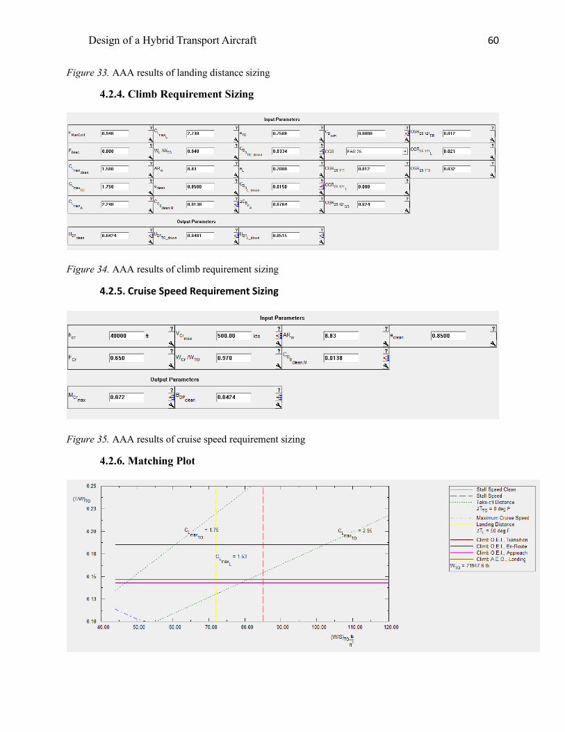
Design of a Hybrid Transport Aircraft 60
Figure 33. AAA results of landing distance sizing
4.2.4. Climb Requirement Sizing
Figure 34. AAA results of climb requirement sizing
4.2.5. Cruise Speed Requirement Sizing
Figure 35. AAA results of cruise speed requirement sizing
4.2.6. Matching Plot

Design of a Hybrid Transport Aircraft 61
Figure 36. AAA results of the performance sizing plot
From the performance sizing plot, a design point with a wing loading of 128.34 lb/ft2 and a thrust
to weight ratio of 0.31 has been chosen. This yelds a 𝐶z�éêè=2.73 , 𝐶z�éê#$
=2.25, 𝑆[ =
560.61𝑓𝑡N, and a thrust of 21,766𝑙𝑏𝑠.
5. Fuselage and Cockpit Design
The cockpit and fuselage design will be modeled after the Boeing 737-100 model aircraft.
Utilizing Roskam’s Airplane Design Part 3, each of these sections will be designed with using
typical arrangements that take into account human factors.
5.1. Cockpit Design
The cockpit will be designed for two pilots with standard heights and weight. The
cockpit will be initially sized to hold two male crew members, as female crew members are
typically smaller. The pilots will be assumed to weigh 175 lbs, based on body component
weights and the fact that they will not be wearing a helmet. For dimensions, the body width
consists of the shoulder width, which will be estimated at 21 in. across, the width at the elbows,
estimated at 22 in. across, and the hip width at 18 in. across. The weights and dimensions include
flight clothing. The remaining dimension assumptions are illustrated in Figure 37, below.

Design of a Hybrid Transport Aircraft 62
Figure 37. Dimensions of sitting male crew member in cockpit (Roskam, 2011).
The cockpit design must also take into account the visibility during takeoff, cruise, and
landing. Figure 37 also illustrates the angles for line of sight. Roskam defines cockpit visibility
as “the angular area obtained by intersecting the airplane cockpit with radial vectors emanating
from the eyes of the pilot” (Roskam, 2011). The point C, in Figure 38, lies on the eyes of the
pilot. Figure 39 demonstrates the minimum visbility pattern for transport aircraft, per FAR 25
specifications.

Design of a Hybrid Transport Aircraft 63
Figure 38. Radial eye vectors emanating from C. (Roskam, 2011)
Figure 39. Ideal minimum visibility pattern for transport aircraft. (Roskam, 2011)
The cockpit layouts in section 5.1.1. meet the visibility requirements and height, width, and
weight requirements for the pilots. They are from the Boeing 737-100 model since the exchange
of the hybrid engine, and battery nacelles will not change the fuselage nor cockpit design.

Design of a Hybrid Transport Aircraft 64
5.1.1. Cockpit Layout Design
Figure 40. Side and top-down view of cockpit. Dimensions in meters (Boeing Commercial Airplanes, 2013)
Figure 41. Front and side 3-D view of cockpit. Dimensions in meters (Boeing Commercial Airplanes, 2013)

Design of a Hybrid Transport Aircraft 65
Figure 42. Rear view of cockpit. (Aircraft Technical Data and Specifications: Boeing 737-100/200, 2017)
5.2. Fuselage Design
5.2.1. Fuselage Layout Design
Figure 43. Top down view of the fuselage (Boeing Commercial Airplanes, 2013)

Design of a Hybrid Transport Aircraft 66
Figure 44. Front view of the fuselage (Boeing Commercial Airplanes, 2013)
Figure 45. Front 3-D view of the 6 abreast passenger seating in the fuselage (Creative Aviation Photography, 2017)

Design of a Hybrid Transport Aircraft 67
Figure 46. Rear 3-D view of the 6 abreast passenger seating in the fuselage (Creative Aviation Photography, 2017)

Design of a Hybrid Transport Aircraft 68
Figure 47. Side view of fuselage with cargo compartment visible (Boeing Commercial Airplanes, 2013)

Design of a Hybrid Transport Aircraft 69
Figure 48. Side view of fuselage with cargo placement (Boeing Commercial Airplanes, 2013)
5.3. Recommendations and Conclusions
5.3.1. Recommendations
In general, the HTA is a hybrid version of the Boeing 737-100. Considering the 96
passenger payload, the 6 abreast seating allows for a smaller fuselage and lower takeoff weight.
The standard cockpit design will work with two pilots, whether male or female. The fuselage
design allows for flight attendant seating.
5.3.2. Conclusions
The current model of the 737-100 fuselage and cockpit meets FAR 25 requirements,
visibility requirements, and provides the opportunity to exchange the engine and add batteries.
To keep the takeoff weight a minimum, the minimum number of passengers will be considered,
and the plane can be expanded length-wise in a future design.

Design of a Hybrid Transport Aircraft 70
6. Wing, High-Lift System and Lateral Control Design
6.1. Wing Planform Design
Using the known gross wing area, S, and aspect ratio, A, the remaining planform design
characteristics of the wing will be chosen. These characteristics include the sweep angle, Λ,
thickness ratio, t/c, airfoil type, taper ratio, λ, incidence angle iw, twist angle, εw, dihedral angle,
Γw, and the lateral control surface size and layout. Some of these will be calculated, and others
will be chosen based on reference data. The HTA will feature conventional, cantilever low wing.
6.1.1. Sweep Angle-Thickness Ratio Combination
The 737-100 has a wing quarter chord sweep angle of 25º and is, therefore, aft swept. The
HTA will feature the same 25 º sweep angle. This angle also matches well with other jet
transport sweep angles, visble in the Figure 49 below.
Figure 49. Jet Transports Wing Geometric Data (Roskam, Airplane Design Part II: Preliminary Configuration Design and Integration of the Propulsion System, 2011)

Design of a Hybrid Transport Aircraft 71
The next values to select for the wing parameters are the taper ratio and the dihedral
angle. The taper ratio consists of the ratio of the tip chord to root chord. The dihedral angel is
the upward angle from the horizontal to the tailplane of the fixed-wing aircraft. These values
will be modeled after the Boeing 737-100. λ=0.339 and Γw=6.
Since the airplane will be flying at high subsonic speeds, a trade study will be performed
varying the sweep angle and the thickness ratio. This will facilitate the choice of the sweep
angle and thickness ratio that allows for the minimum weight of the wing. The following
equation:
���� BX9� (
)tÚ���� BX9� (*¬+�t
Ní
N.©¤¬|�
BX9 (î + ¬+�t
Ní
N.©¤¬|�(Ë.u¤�^)
BX9ì (î,+ ���� BX9� (
tÚ���� BX9� (-¬+�t
Ní
t.uN¬|�
BX9(îN
.+𝑀BBN 𝑐𝑜𝑠N 𝛬 Ù1 +
¬+�tN (Ë.©¦B^)BX9� (
+ ¬+�tN (Ë.u¤B^)BX9� (
Ý − 1 = 0 (39)
can be used to solve for the thickness ratio for varying sweep angles. The table and plot below
demonstrate these results.
Table 28. Thickness Ratio and Wing Weight vs. sweep angle Λ (deg) t/c Ww (lbs) 0 0.079 ---------- 5 0.081 436448.0332 10 0.086 81961.74273 15 0.095 44021.92291 20 0.108 29471.24401 25 0.124 21783.48296 30 0.145 17064.19453 35 0.169 13911.36935 40 0.197 11691.97308 45 0.227 10076.63814 50 0.259 8877.443908 55 0.291 7981.378457 60 0.319 7320.729094 65 0.338 6862.089862 70 0.337 6614.330935 75 0.295 6700.319668 80 0.142 8184.063457 85 -0.454 ----------
Figure 50. Plots of t/c and Ww vs. Λ
02000400060008000
1000012000
0 50 100
Win
g W
eigh
t (lb
s)
Λ (deg)
Wing weight vs. Sweep Angle
0.000
0.250
0.500
0 50 100
t/c
Λ (deg)
t/c vs. Λ

Design of a Hybrid Transport Aircraft 72
Using the wing weight as the figure of merit, the minimum wing weight occurs at a
sweep angle of 70º. This is not a reasonaible sweep angle, and therefore, the wing weight may
not be an appropriate figure of merit.
Besides using the weight of the wing as a figure of merit, there are other considerations
for selecting the thickness ratio. The thickness ratio should be greater than 0.1 to accommodate
the wing structure, fuel, batteries, and main landing gear when retracted. Additionally the
thickness ratio should not exceed 0.2 in order to prevent the drag profile from being too high.
Additionally, large sweep angles result in lower performance of the wing during low speed. As a
result, high lift systems may be necessary to improve this performance. Using these values for
the thickness ratio, a sweep angle between 20 and 40º would be appropriate. Thus, the 25º angle
will be selected and this results in a thickness ratio of 0.124.
6.2. Airfoil Selection
Selecting the airfoil involves considering the aircraft mission, along with properties of the
drag coefficient at the design lift coefficition, section critical Mach number, and section pitching
moment. The Boeing 737-100 used the Wing root- BAC 449/450/451 airfoil with Wing tip-
BAC 442 airfoil . This will be selected as well for the HTA. The schematic, below, illustrates
the various airfoils for the root airfoil, two midspan airfoils, and outbard airfoil.
Figure 51. Boeing 737 Airfoil selections schematic (Aircraft Technical Data and Specifications: Boeing 737-100/200, 2017)

Design of a Hybrid Transport Aircraft 73
Based on Roskam’s wing geometric data for transport aircraft, the incidence angle will be
1º (Aircraft Technical Data and Specifications: Boeing 737-100/200, 2017). Using the Boeing
737-100 model, the dihedral angle used will be 6º. Most aircraft have negative wash-out twist
angles. Based on Roskam’s discussion of designing wings for transport aircraft, a twist angle of -
2º will be assumed.
6.3. Design of the High-Lift Devices
High lift devices are useful to help the aircraft meet its requirements for 𝐶z0*0 ñòand
𝐶z0*0 z. High lift devices include leading-edge devices and trailing-edge devices. Leading edge
devices include VC Krueger flap, two-position slat, three-position slat, fixed slot, variable
camber (VC) leading edge, hinged leading edge (or droop nose), folding bull-nose Krueger flap
(Rudolph, 1996). Trailing edge devices include split flap, plain flap, simple slotted flap, single-
slotted Fowler flap, fized vain/main slotted flap, articulating vane/main double slopped flap,
main/aft double slotted flap, triple-slotted flap (Rudolph, 1996).
The following sizing will determine which high lift devices would provide the HTA with
enough lift to meet the takeoff and landing mission requirements. The HTA has 𝐶z�éêè=2.73 and
𝐶z�éê#$=2.25. These values were determined from the performance sizing in discussed in
Chapter 4. According to Roskam, sizing the high lift devices involves determining the maximum
lift coefficient capability of the wing, estimating ∆𝐶z�éê#$ and ∆𝐶z�éêè
, accounting for the
sweep of the wing, and then sizing the device using the desired ∆𝐶z. Using the planform design
characteristics of Λ=25º, t/c= 0.124, λ=0.339, iw =2º , εw=, Γ=6º, S=1098 ft2, b=93 ft, cr=24.02
ft , and ct= 5.2 ft, the high lift devices will be sized.
The 𝐶z�éê can be obtained from the 𝐶z�éê1 . To calculate the maximum lift coefficient
of the wing, the following equation will be used:

Design of a Hybrid Transport Aircraft 74
𝐶z�éê1 =ë2Ç�è�éê ���è�éê |É
N (40)
Thus, using k4 = 0.957 and obtaining the root and tip maximum lift coefficients for the airfoil,
𝐶z�éê1 can be calculated, with 𝐶z�éê1 = Ë.§¨¥(t.§�t.©)N
= 1.67.
Figure 52. Cl vs. angle of attack for maximum lift coefficient at root and midspan
𝐶z�éê1 = 1.1, and taking into account the quarter chord sweep angle, 𝐶z�éê1 = 1.8.
Since the original 737-100 is a short-coupled airplane, the HTA will be assumed to be a short-
coupled airplane. Therefore,
𝐶z�éê1 = 1.1𝐶z�éê (41)
and 𝐶z�éê = 1.6.
Using 𝐶z�éê = 1.6, the ∆𝐶z�éê1 and ∆𝐶z�éêè can be calculated using the following two
equations.
∆𝐶z�éê#$ = 1.05(𝐶z�éê#$− 𝐶z�éê ) (42)
∆𝐶z�éêè = 1.05(𝐶z�éêè− 𝐶z�éê ) (43)
Therefore, ∆𝐶z�éê#$ = 1.05(2.25 − 1.1) = 1.2 and ∆𝐶z�éêè = 1.05(2.73− 1.1) = 1.7. The
factor of 1.05 takes into account the trip penalties incurred when using flaps. To calculate the

Design of a Hybrid Transport Aircraft 75
∆𝐶z�éêvalues, with the sweep correction factor taken into consideration, the following table
illustrates the various ∆𝐶z�éêwith three arbitrary flapped wing area to wing area ratios.
Table 29. ∆C56789: and ∆C5678; using various Swf/S
Takeoff Landing Swf/S ∆𝑐$�éê#$ ∆𝑐$�éê; 0.60 0.83 1.18 0.80 1.11 1.57 0.90 1.25 1.77
In order to achieve the required flap lift increments, Fowler flaps will be used. The
Fowler flaps have the following geometry: B<B= 0.3, 𝛿=|ÿ = 35°,𝛿=è = 40°. (Roskam, Airplane
Design Part II: Preliminary Configuration Design and Integration of the Propulsion System,
2011). The required incremental section lift coefficient, ∆𝑐) will be calculated. This is the value
that the trailing edge flaps must generate. The∆𝑐)�éê values have been estimated at takeoff and
landing based on the Swf/S ratio. ∆𝑐) is related to ∆𝑐)�éê through the following equation
∆𝑐$ = ¬t?∆𝑐$�éê (44)
K=0.94 is determined using , below, with 𝑐=/𝑐 = 0.3 Thus the needed ∆𝑐)values can be
summarized in Table 30.
Figure 53. Effect of Flap Chord Ratio and Flap Type on K

Design of a Hybrid Transport Aircraft 76
Table 30. Calculated∆𝑐$ for takeoff and landing
Takeoff Landing Swf/S ∆𝑐)YX ∆𝑐)$ 0.60 0.88 1.26 0.80 1.18 1.67 0.90 1.33 1.88
For Fowler flaps, the following equations hold:
∆𝑐$ = 𝑐$∝∝@<A< (45)
𝑐$B< = 𝑐$∝(BC/B) (46)
BC
B= 1 + 2¬
D<UB 𝑡𝑎𝑛 ¬
A<N (47)
Therefore, ∆𝑐) = 2𝜋(0.53) ¬ u¨¨¥.N§
= 2.03. Finally, using
�F<�= (𝜂Ë − 𝜂"){2 − (1 − 𝜆)(𝜂" + 𝜂Ë)}/(1 + 𝜆) (48)
the following is a summary of the flap geometry: �F<�= 0.83,
B<B= 0.3, 𝛿=|ÿ = 35°,𝛿=è = 40°.
The ∆𝑐) supplied by the Fowler flaps satisfies the required ∆𝑐)for both takeoff and landing.
Thus, the Fowler flaps will be sufficient in providing additional lift.
6.3.1. AAA Calculation of Lift Coefficient
Using AAA, the clean maximum lift coefficient was found to be 1.541. Although this
value is lower than the original manual calculations, the increase in lift provided by the Fowler
Flaps is still substantial to provide the aircraft with lift.
Figure 54. AAA Estimate of clean Lift Coefficient of the Wing

Design of a Hybrid Transport Aircraft 77
6.4. Design of the Lateral Control Surfaces
Roskam provides reference data for the lateral control surfaces. The data for jet
transports is summarized in the table below. The aircraft will have a rudder area of 56.2 ft2, a fin
height of 20.2 ft, and a fin area of 224 ft2 . The HTA will also have ailerons and spoilers with the
ailerons composing 2.4% of the wing area.
In summary, the HTA will have the following wing parameters: b=93 ft, cr=24 ft, ct=5.2
ft, mac=12.5 ft, mgc=12.5 ft, ΛLE=27.8º , ΛTE= 16.625º, and (40.7, 43.8)= coordinates of the
aerodynamic center measured in feet from the center of gravity.
The following figures will illustrate the wing planform and show these parameters.
Table 31. Jet Transport Lateral Control Surface Information

Design of a Hybrid Transport Aircraft 78
Table 32. Additional Jet Transport Lateral Control Surface Information

Design of a Hybrid Transport Aircraft 79
6.5. Drawings
Figure 55. Wing Planform: flap and lateral control layout
6.6. Discussion
The HTA planform and lateral control layout illustrate the wing parameters. The Fowler
flaps will be full span, and the spoilers will be used for lateral control. The spoilers will run
from 0.4(RN)to 0.66¬R
N with 0.14c to 0.18c. The outboard ailerons will run from 0.74¬R
N to
0.94¬RN with 0.20c to 0.28c. Additionally, the drawings demonstrate the span of 93 feet, and the
root and tip chord.
Design of a Hybrid Transport Aircraft 80
6.7. Recommendations and Conclusions
6.7.1. Recommendations
Based on the geometry of the wing and the flight parameters chosen, Fowler flaps are the
recommended high lift device that will provide substantial lift. Additionally, the fuel can be
stored in the wing without the risk of fire due to lightning strikes since the fuel in the HTA is less
than the fuel in the 737-100. The batteries will additionally be suspended below the wing in
nacelles, and this may change the aerodynamics surrounding the flaps and the nacelles.
6.7.2. Conclusions
The data in both tables from Roskam, along with pre-existing Boeing 737-100
specifications, provides benchmarks with which to compare the wing parameters. Although
wing weight is usually a figure of merit for the thickness ratio, it proved to be a poor basis for the
thickness ratio. Using a thickness ratio greater than 0.1 and less than 0.2 proved to provide
optimal sweep angles of 25º at the quarter chord, along with a reasonable thickness ratio of
0.124. Additionally. The 25º sweep angle, which is the same as the original 737-100, yielded
ΛLE=27.8º , ΛTE= 16.625º, from linear interpolation.
Through the analysis of the Boeing airfoil data, the ∆𝐶z�éê was calculated, and the
Fowler flaps were found to provide substantial lift, without any leading edge devices. The HTA
has requirements for 𝐶z678 ÔG = 2.25 and 𝐶z678; = 2.73. The calculations demonstrated that an
additional ∆𝐶z�éê of 1.25 is needed for takeoff and ∆𝐶z�éêof 1.77 is needed for landing. Since
the Fowler flaps provide an additional ∆𝐶z�éê = 2.03, they are substantial in providing lift.
Other high lift devices could be considered for the HTA. Given the geometry of the wing
and the parameters chosen, the Fowler flaps provide adequate lift, and the wing geometry
provides adequate storeage for the fuel.

Design of a Hybrid Transport Aircraft 81
7. Design of the Empennage and the Longitudinal and Directional Controls
7.1. Overall Empennage Design
The empennage design, which was initially introduced in the configuration design
chapter is composed of the tail and stabilizing features organized in a tail aft arrangement. The
HTA will feature a single vertical tail mounted to the fuselage along with a horizontal stabilizer.
For conventional configurations, the center of mass is generally near wing’s aerodynamic
center. This is the point at which the wing’s pitching moment coefficient doesn’t vary with
changes in angle of attack. The empennage moment arms, 𝑥@, 𝑥8, 𝑥B, will be located so as to
create a maximum moment arm relative to the center of gravity (Roskam, Airplane Design Part
III: Layout Design of Cockpit, Fuselage, Wing, and Empennage: Cutaways and Inboard Profiles,
2011). Besides creating a large moment arm, the placement of these locations minimizes the
area of the empennage. This helps minimize the weight of the aircraft and the drag during flight.
For the HTA, 𝑥@ = 43.8𝑓𝑡𝑎𝑛𝑑𝑥8 = 40.7𝑓𝑡. The in the table below summarizes the volume
coefficients and control surface data.
Table 33. Summary of Comparable Volume Coefficients and Control Surface Data
U
s
i
n
g
c
𝑆@ = 𝑉@PPP𝑆𝑐 ̅/𝑥@ (49)
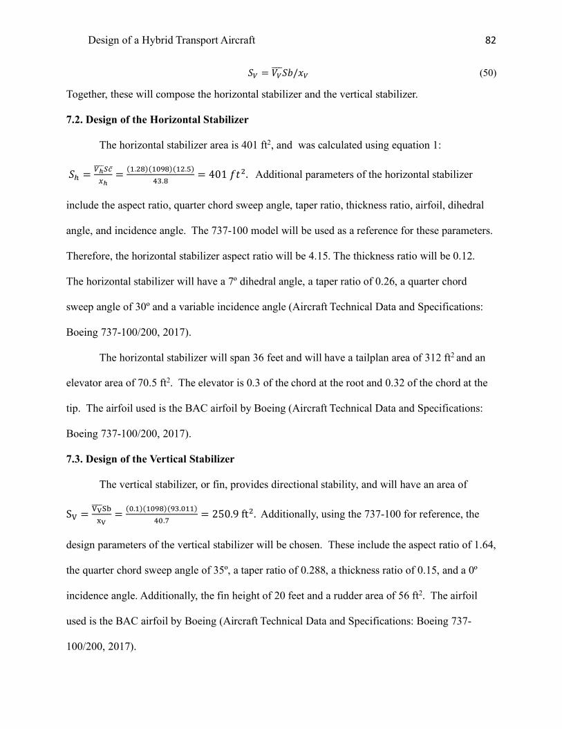
Design of a Hybrid Transport Aircraft 82
𝑆~ = 𝑉~PPP𝑆𝑏/𝑥~ (50)
Together, these will compose the horizontal stabilizer and the vertical stabilizer.
7.2. Design of the Horizontal Stabilizer
The horizontal stabilizer area is 401 ft2, and was calculated using equation 1:
𝑆@ =~UPPPP�B ̅LU
= (t.N¦)(t˧¦)(tN.¨)¤u.¦
= 401𝑓𝑡N. Additional parameters of the horizontal stabilizer
include the aspect ratio, quarter chord sweep angle, taper ratio, thickness ratio, airfoil, dihedral
angle, and incidence angle. The 737-100 model will be used as a reference for these parameters.
Therefore, the horizontal stabilizer aspect ratio will be 4.15. The thickness ratio will be 0.12.
The horizontal stabilizer will have a 7º dihedral angle, a taper ratio of 0.26, a quarter chord
sweep angle of 30º and a variable incidence angle (Aircraft Technical Data and Specifications:
Boeing 737-100/200, 2017).
The horizontal stabilizer will span 36 feet and will have a tailplan area of 312 ft2 and an
elevator area of 70.5 ft2. The elevator is 0.3 of the chord at the root and 0.32 of the chord at the
tip. The airfoil used is the BAC airfoil by Boeing (Aircraft Technical Data and Specifications:
Boeing 737-100/200, 2017).
7.3. Design of the Vertical Stabilizer
The vertical stabilizer, or fin, provides directional stability, and will have an area of
SJ =JKPPPPL+0K
= (Ë.t)(t˧¦)(§u.Ëtt)¤Ë.¥
= 250.9ftN. Additionally, using the 737-100 for reference, the
design parameters of the vertical stabilizer will be chosen. These include the aspect ratio of 1.64,
the quarter chord sweep angle of 35º, a taper ratio of 0.288, a thickness ratio of 0.15, and a 0º
incidence angle. Additionally, the fin height of 20 feet and a rudder area of 56 ft2. The airfoil
used is the BAC airfoil by Boeing (Aircraft Technical Data and Specifications: Boeing 737-
100/200, 2017).

Design of a Hybrid Transport Aircraft 83
7.4. Empennage Configuration Drawings
The figure below consists of the drawings of the empennage arrangement for the HTA.
Included in this drawing are the elevator and rudder outlines. All dimensions are in feet and are
illustrated below.
Figure 56. Empennage Configuration (units in feet)

Design of a Hybrid Transport Aircraft 84
7.5. Empennage Design Evaluation
AAA will be used to analyze the performance of the empennage horizontal and vertical
stabilizers. Using the inputs of AP, λ, S, Λc/4, and the x, y, and z offset values, the output
parameters were calculated. This provided the root and tip dimensions, span, mean geometric
chord, leading edge and trailing edge sweep angle, and the positions for the mean geometric
chord for both the vertical and horizontal tail. The outputs and inputs are presented below.
Figure 57. Horizontal Tail Geometry Calculations by AAA
Figure 58. Vertical Tail Geometry Calculations by AAA
Design of a Hybrid Transport Aircraft 85
7.6. Discussion
Since the use of batteries during various stage of flight will not change the empennage,
the 737-100 model was used as a reference for the HTA. This data, along with similar data
provided by Roskam, provided the foundation for initial selections for the parameters.
Additionally, the parameters chosen are consistent with the control surface ratios provided by
Roskam. Thus, 𝑆6/𝑆@ = 0.27 for a 737-200 and 𝑆6/𝑆@ = 0.24 for a 737-300. Using the 737-
100 parameters, �J�U= ¥Ë.¨
¤Ët= 0.18. This value is lower, but comparable. For the rudder area to
vertical stabilizer area, ���V= 0.31𝑎𝑛𝑑0.39 for 737-200 and 737-300, respectively. For the HTA,
���V= ¨©
N¨Ë.§= 0.22. Again, although this is lower, it is comparable.
AAA additionally calculated very similar values to the original 737-100 aircraft. The tail
geometry is consistent with previous aircraft, and will provide adequate stability for the HTA.
7.7. Recommendations and Conclusions
7.7.1. Recommendations
The HTA empennage will be modeled after the 737-100 airplane with slight changes.
The moment arms have been estimated at 𝑥@ = 43.8𝑓𝑡𝑎𝑛𝑑𝑥8 = 40.7𝑓𝑡. These locations will
be iterated to determine the aerodynamic center that provides the best stability and control.
7.7.2. Conclusions
The tail aft empennage arrangement provides a suitable conventional configuration
design for the HTA. With the hybrid plane being modeled after the 737-100, the parameters have
been chosen based on the fuel powered model. The distance from the cg to the ac will be
established further when exploring the stability and control of the landing gear and may be
adjusted, if necessary, after an iterative process. The figures below illustrate how the empennage
fits in the aircraft.
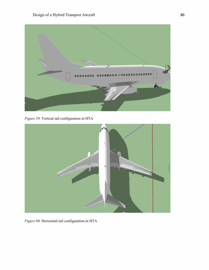
Design of a Hybrid Transport Aircraft 86
Figure 59. Vertical tail configuration in HTA
Figure 60. Horizontal tail configuration in HTA

Design of a Hybrid Transport Aircraft 87
8. Design of the Landing Gear and Weight and Balance Analysis
8.1. Introduction
The landing gear arrangement, previously introduced in the configuration chapter, will
consist of retractable conventional tricycle landing gear. The main landing gear will retract into
the fuselage, and the nose landing gear will retract into the nose. In order to size the landing gear,
the center of gravity will need to be determined. From there, a weight and balance iteration will
be performed to determine whether the cg of the proposed design is in the correct location. The
cg excursion diagram will be used to illustrate the possible locations of the cg.
8.2. Estimation of the Center of Gravity
The following data consists of the component weight and coordinate data for the Class I
component weight estimation Assuming a takeoff weight of 83,000 lbs and the weight fractions
from Roskam’s Part V. Component Weight Estimation, the weights and positions are summarized
in the table below (Roskam, Airplane Design Part II: Preliminary Configuration Design and
Integration of the Propulsion System, 2011).
The zero reference point will be located a distance well to the left and below the airplane.
This allows the airplane to change size without changing the reference point. The x-axis will
refer to x-coordinates called the fuselage stations (F.S.) and the y-axis coordinates will be
referred to as the wing buttock lines (B.L.). For the HTA, the first F.S. point will be at 151
inches, and the first B. L. point will be at 78 inches.
The comcomponent weight and coordinate data for the HTA are summarized in Table 34,
below. Note that the aircraft is symmetric, so the y coordinates will all be 0 inches.

Design of a Hybrid Transport Aircraft 88
Table 34. HTA Component Weight and Coordinate Data
No. Type of Component
Wi (lbs) xi (in.)
Wixi (in lbs)
yi (in.)
Wiyi (in lbs)
zi (in.) Wizi (in lbs)
1 Fuselage Group
8,549 641 5,479,909 0 0 248 2,120,152
2 Wing Group 7,636 680 5,192,480 0 0 350 2,672,600 3 Empennage
Group 1,992 1190 2,374,480 0 0 300 597,600
4 Engine Group
20,950 590 12,360,500 0 0 140 2,933,000
5a Landing Gear Group:Nose Gear
500 390
195,000
0 0 130
74,750
5b Landing Gear Group: Main Gear
2654 710 1,884,340
0 0 130 345,020
6 Fixed Equipment Group
10,707 680 7,280,760
0 0 200 2,141,400
7 Trapped Fuel and Oil
142.8 690 98,532 0 0 215 30,702
8 Crew 700 300 210,000 0 0 240 168,000 9 Fuel 4,500 690 3,105,000 0 0 430 1,935,000 10 Batteries 18,000 733 13,194,000 0 0 120 2,160,000 11 Passengers 16,800 680 11,424,000 0 0 200 3,360,000 12 Luggage 3,000 680 2,040,000 0 0 200 600,000

Design of a Hybrid Transport Aircraft 89
Figure 61. c.g. for various aircraft components

Design of a Hybrid Transport Aircraft 90
Figure 62. c.g. location for each component on the aircraft
Using the listed c.g. locations for the various components and their individual weights,
the c.g. excursion diagram was produced using Excel. The most forward c.g. is located at 46.91
ft. and the most aft c.g. is located at 66.08 ft. Although they have a very wide spread, AAA will
be used to check these calculations, and then after the landing gear placement, the weight and
balance will be performed again.

Design of a Hybrid Transport Aircraft 91
Figure 63. c.g. excursion plot produced using Microsoft Excel
Using the 737-200 airplane for comparison, the weight fractions were calculated for the
various components. The figure below illustrates the results from AAA.
Figure 64. Weight fractions referenced from the 737-200 from AAA
Using the empty weights, the c.g. positions for each of the empty weight components can
be determined, as well as the c.g. of the structure as a whole. These results, from AAA, are
summarized as follows.
0
10000
20000
30000
40000
50000
60000
70000
80000
90000
100000
650 700 750 800 850 900 950
Wei
ght (
lbs)
F.S. (in)
c.g. Excursion Diagram

Design of a Hybrid Transport Aircraft 92
Figure 65. c.g. locations produced using AAA
Using the outputted parameters as inputs, the c.g. of the HTA along with the c.g. locations
for each component.
Figure 66. c.g. location for MTOW aircraft
From here, the c.g. excursion diagram for the x and z directions can be plotted. The
following information was used to plot the c.g. excursion diagram.

Design of a Hybrid Transport Aircraft 93
Figure 67. Loading Table from AAA for x-direction c.g. excursion diagram
Using the loading table and the valculated c.g. values, the x c.g. excursion plot illustrates
the possible c.g. locations depending on the loading scenario.
Batteries

Design of a Hybrid Transport Aircraft 94
Figure 68. c.g. excursion diagram (x-direction)
The plot illustrates a variation in c.g. with the most forward c.g. being located at 22.9 ft
and the most aft c.g. being located at 35.7 ft. Note that the c.g. is left of the main landing gear,
which indicates that the HTA will not tip over with the current loading and unloading scenarios.
For reference, the z-direction c.g. excursion diagram has also been plotted. Note that for the
loading and unloading scenarios, the cargo represents the batteries.

Design of a Hybrid Transport Aircraft 95
Figure 69. Loading Table from AAA for z-direction c.g. excursion diagram
Figure 70. c.g. excursion diagram (z-direction)
Batteries
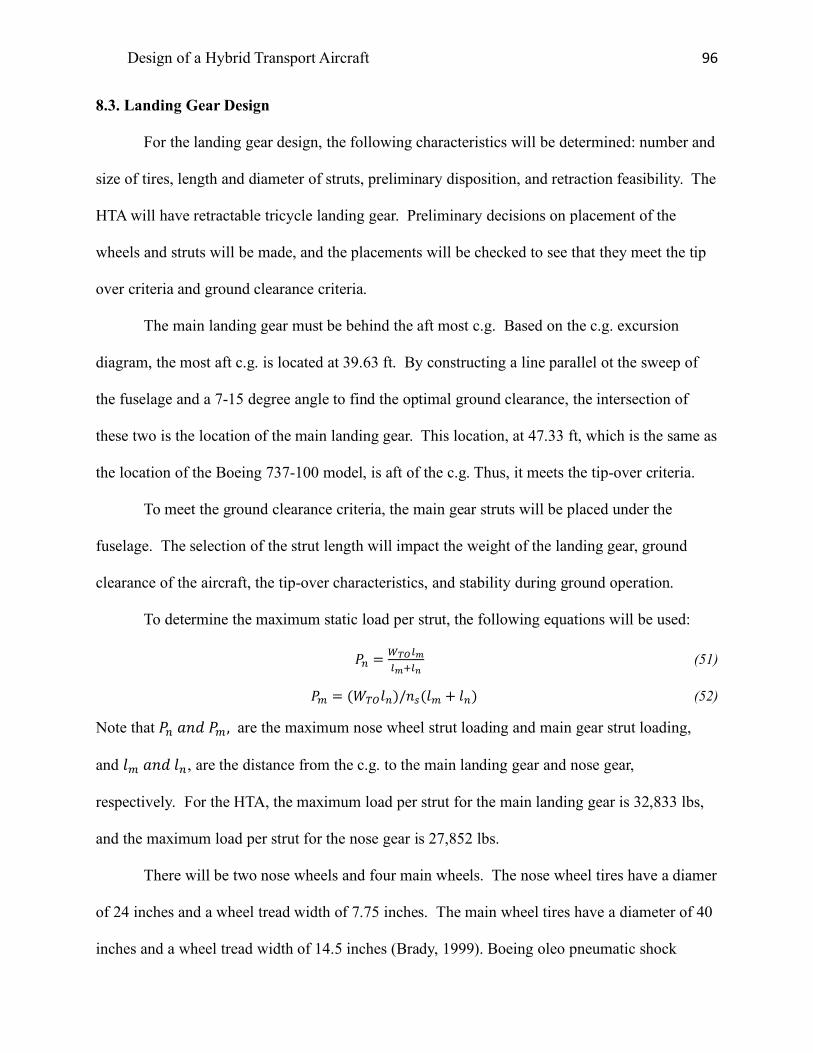
Design of a Hybrid Transport Aircraft 96
8.3. Landing Gear Design
For the landing gear design, the following characteristics will be determined: number and
size of tires, length and diameter of struts, preliminary disposition, and retraction feasibility. The
HTA will have retractable tricycle landing gear. Preliminary decisions on placement of the
wheels and struts will be made, and the placements will be checked to see that they meet the tip
over criteria and ground clearance criteria.
The main landing gear must be behind the aft most c.g. Based on the c.g. excursion
diagram, the most aft c.g. is located at 39.63 ft. By constructing a line parallel ot the sweep of
the fuselage and a 7-15 degree angle to find the optimal ground clearance, the intersection of
these two is the location of the main landing gear. This location, at 47.33 ft, which is the same as
the location of the Boeing 737-100 model, is aft of the c.g. Thus, it meets the tip-over criteria.
To meet the ground clearance criteria, the main gear struts will be placed under the
fuselage. The selection of the strut length will impact the weight of the landing gear, ground
clearance of the aircraft, the tip-over characteristics, and stability during ground operation.
To determine the maximum static load per strut, the following equations will be used:
𝑃# ={#$$�$��$I
(51)
𝑃E = (𝑊ñò𝑙#)/𝑛9(𝑙E + 𝑙#) (52)
Note that 𝑃#𝑎𝑛𝑑𝑃E, are the maximum nose wheel strut loading and main gear strut loading,
and 𝑙E𝑎𝑛𝑑𝑙#, are the distance from the c.g. to the main landing gear and nose gear,
respectively. For the HTA, the maximum load per strut for the main landing gear is 32,833 lbs,
and the maximum load per strut for the nose gear is 27,852 lbs.
There will be two nose wheels and four main wheels. The nose wheel tires have a diamer
of 24 inches and a wheel tread width of 7.75 inches. The main wheel tires have a diameter of 40
inches and a wheel tread width of 14.5 inches (Brady, 1999). Boeing oleo pneumatic shock

Design of a Hybrid Transport Aircraft 97
aborbers provide shock absorption. One main gear strut and one nose gear strut dampen the
vertical oscillations felt upon landing.
Figure 71. Landing gear and strut placement
Figure 72. Nose gear retraction

Design of a Hybrid Transport Aircraft 98
Figure 73. Stick Diagram for main gear retraction
Figure 74. Illustration of the two nose tires and four main tires for the landing gear.
Figure 75. Landing Gear retracted into fuselage

Design of a Hybrid Transport Aircraft 99
8.4. Weight and Balance
Since the landing gear placement, at 47 feet from the nose, is aft of the most aft c.g., the
weight and balance does not need to be repeated. The location of the main landing gear
correlates with the location of the main landing gear in the 737-100 model.
8.5. Conclusion
Compared to the 737-100 model, the c.g. excursion diagram demonstrated the change in
c.g. location due to the addition of the batteries. The location of the batteries did not change the
location of the main landing gear, and, as a result, the HTA will not tip over in any loading
scenario. The landing gear can support the weight of the plane, with the added weight due to the
batteries, and the landing gear retracts directly into the fuselage.
9. Stability and Control Analysis
9.1. Introduction
The stability and control analysis will be performed by following Roskam’s steps in
Airplane Design Part II. This will allow the determination of the stability and control
characteristics of the HTA. These characteristics include the static longitudinal stability, static
directional stability, and minimum control speed with one engine out (Roskam, Airplane Design
Part II: Preliminary Configuration Design and Integration of the Propulsion System, 2011)
Stability is the tendency of an object to return to equilibrium when displaced (Crawford,
2009). Static stability involves an object’s initial tendency to return to equilibrium upon initial
displacement. For aircraft, this requires a balance because the greater an aircraft’s static stability,
the greater its resistance in maneuvering. The center of gravity, or c.g., strongly determines the
longitudinal static stability. Moving the c.g. aft reduces static stability and increases
maneuverability.

Design of a Hybrid Transport Aircraft 100
Aircraft can have inherent stability, in which the stability is built into the aircraft’s design,
or de facto stability, where control systems provide feedback and provide stability requirements.
Some aircraft have relaxed stability. This type of stability involves the aircraft changing its
attitude and bank angle on its own. This, along with stability augmentation devices, allows for
better cruise performance and better maneuverability at high altitudes. Many jet transport
aircraft have relaxed stability. The HTA will also feature relaxed stability.
9.2. Static Longitudinal Stability
The longitudinal X-plot illustrates the rate at which the c.g. moves aft as a function of the
horizontal tail area and the rate at which the aerodynamic center, or a.c., moves aft as a function
of the horizontal tail area. This will be plotted for the HTA, which features a conventional
configuration.
The a.c. leg of the plot will be calculated using the following equations:
�̅�4BÛ =OL̅é�F<�
�PèBUªÁQÆRUÆB «ª
ýUý «êSé�UQPèB�ªÁÃ
ÆR�ÆB «êSé��¬
ý�ý �
P ��èBF<T
ó (53)
𝐹 =*t�(�èBU¬tÚ
ÆRUÆB ¬
ýUý ��èB�¬t�
ÆR�ÆB ¬
ý�ý î]
�èBF< (54)
The figure below illustrates how to find the geometric quantities to perform these calculations.
(Roskam, Airplane Design Part II: Preliminary Configuration Design and Integration of the
Propulsion System, 2011)

Design of a Hybrid Transport Aircraft 101
Figure 76. Geometric quantities for aircraft calculations
Figure 77. Longitudinal X-Plot for the HTA
The longitudinal x plot illustrates that as the tail plane area is increased, the c.g. moves
aft, and the a.c. also moves aft, but more slowly. The 10% difference between the a.c. and c.g.
location is the optimal area of the horizontal stabilizer.
The 10% static margin yields a horizontal stabilizer area of 380-401 ft2. These results
match the results from the wing design, where the horizontal stabilizer area was sized to 401 ft2.
0
200
400
600
800
1000
1200
0 50 100 150 200 250 300 350 400 450
c.g.
and
a.c
. mov
emen
t (in
)
horizontal tail area (ft^2)
Longitudinal X-Plot

Design of a Hybrid Transport Aircraft 102
This yields a slightly larger wing area than the 737-100, but this is likely due to the extra battery
weight being suspended below the wings.
The HTA has a level of instability of 0.085𝑐[̅, which has been chosen based on the
instability levels of comparable jet transport. Using the aft c.g. leg of the longitudinal X-plot, the
longitudinal stability augmentation system must generate a change in static margin of ∆𝑆𝑀 =
0.085 + 0.05 = 0.135, where the minimum static margin of 𝑋PB7 − 𝑋P4B = 0.05 or 5%. The
empennage area follows from these calculations. The original horizontal tail area of 401 ft2 will
be compared with the horizontal tail area obtained from the longitudinal X-plot. Since they are
the same, 401 ft2 will remain the design size.
9.3. Static Directional Stability
The directional X-plot illustrates the change in directional stability for various vertical
tail areas.
Figure 78. HTA Directional X-Plot
The desired de facto level of directional instability is C&W = 0.0010. From the plot,
𝐶#X = −0.001 and there is a difference of 0.002. The sideslip feedback system must support
-0.005
-0.004
-0.003
-0.002
-0.001
0
0.001
0.002
0 50 100 150 200 250 300
C_n_
b (1
/deg
)
Vertical Tail Area (ft^2)
Directional X-Plot

Design of a Hybrid Transport Aircraft 103
this difference. To compute the required sideslip to rudder feedback gain, the following
equations will be used.
𝑘Y =∆�IX�I@�
, with 𝑘Y < 5𝑑𝑒𝑔/𝑑𝑒𝑔 (55)
∆𝐶#X = 0.0010 − 𝐶#X (56)
As a result, k[ =∆\ÖW\Ö'(
= Ë.ËËtËÚË.ËËNÚË.ËËtN
= 0.833𝑑𝑒𝑔/𝑑𝑒𝑔. This is acceptable, and the
vertical tail is not critical for the HTA.
9.4. Minimum Control Speed with One Engine Inoperative
The critical one engine out yawing moment can be determined from the following
equation.
𝑁Y���| = 𝑇ñòJ𝑌Y (57)
In this equation 𝑌Yis the lateral thrust moment arm of the most critical engine, which equals 17.5
ft. T̂ _Õ is the thrust required by the engine at takeoff. The geometry for these calculations is
illustrated in the figure below.
Figure 79. Geometry for one engine out Vmc calculations

Design of a Hybrid Transport Aircraft 104
Using the geometry and the thrust at takeoff, N1a(bÔ = T̂ _ÕY1 = 21,000𝑙𝑏 ∙ 17.5𝑓𝑡 =
367,500𝑓𝑡𝑙𝑏𝑠. For a jet transport with a low bypass ratio, 𝑁w = 0.15𝑁Y���|, and thus 𝑁w =
55,125𝑓𝑡𝑙𝑏𝑠. Therefore, the critical engine out yawing moment is 55,125 ft lbs.
The following equations can be used to calculate the maximum allowable 𝑉EB and the
rudder deflection required to hold the engine out condition at 𝑉EB . The rudder deflection angle
should not exceed 25 degrees. If it does, the vertical tail needs to be resized or the rudder needs
to be resized.
𝑉EB = 1.2𝑉9 (58)
𝛿T = (𝑁w + 𝑁Y���|)/𝑞PEB𝑆𝑏𝐶#@� (59)
Using the lowest stall speed, which is the stall speed at landing, 𝑉EB is calculated to be 1.2V�; =
1.2(54) = 64.8𝑘𝑡𝑠. From the vertical tail and rudder geometry, the control power derivative is
equal to C&'( = −0.245𝑟𝑎𝑑Út. Thus, at V0e = 64.8kts, the rudder deflection angle is
calculated to be 𝛿T =ñ#$Jf|
Ú%P�R\Ö'(.
δ� = (Nh + N1a(bÔ)/qP0eSbC&'( = (55,125𝑓𝑡𝑙𝑏𝑠 + 367,500𝑓𝑡𝑙𝑏𝑠)(.5(7.38 ∗
10Ú¤)(109.37𝑓𝑡/𝑠)N(250𝑓𝑡N)(93.011𝑓𝑡) ¬− Ë.ËËtN367
= 43.6º. This is a large angle, and the
size of the vertical tail should be increased and the calculation performed again.
9.5. Empennage Design-Weight and Balance- Landing Gear Design- Longitudinal Static
Stability and Control Check
The horizontal stabilizer area meets the 10% static margin difference, and the horizontal
stabilizer does not need to be resized. The vertical stabilizer needs to increase in order to provide
a smaller rudder deflection angle.

Design of a Hybrid Transport Aircraft 105
9.7. Conclusion
Overall, the sizing of the HTA is still comparable to the 737-100 model. The horizontal
stabilizer was increased to 401 ft2, as determined in the wing sizing chapter, and this sizing will
be maintained based on the longitudinal X-plot.
The critical one engine out yawing moment has been determined to be 55,125 ft lbs, with
a minimum control speed of 64.8 kts.
Rudder deflection should not exceed 25 degrees, but was calculated to be 43.6°, whichi
necessitates an increase in size of the vertical stabilizer. This will be explored further during the
Class II sizing.
10. Drag Polar Estimation
10.1. Introduction
A drag polar is the relationship between the airplane’s lift and its drag, where the lift
coefficient depends on the drag coefficient. The results of the HTA’s comparison of its lift and
drag coefficients will be examined and displayed in a plot.
To perform the drag polar estimation, Roskam’s method will be utilized. This involves
eight steps. Initially, the wetted area of the airplane components will be estimated. The airraft’s
components will be analyzed individually. These include the fuselage, wings, empennage, and
engine and battery nacelles. Once these have been computed, the equivalent parasite area will be
calculated. From there, the compressibility drag increment will be found along with the flap
drag increment, and landing gear drag increment. The drag polars for cruise, takeoff, and
landing will be constructed, and the L/D critical values will be determined from the drag polars.
10.2. Airplane Zero Lift Drag
The following equations will be used to compute the wetted areas for each component.

Design of a Hybrid Transport Aircraft 106
𝑆[6Y5$= = 2𝑆6L5.5$={1 + 0.25 ¬YBT(1 + 𝜏𝜆)/(1 + 𝜆). (60)
𝜏 = ¬YBT/ ¬Y
BY (61)
𝜆 = 𝑐Y/𝑐� (62)
𝑆[6Y=>9 = 𝜋𝐷=𝑙= ª1 −Nl<«�ì(1 + 1/𝜆=N) (63)
𝜆= = 𝑙=/𝐷= (64)
𝑆[6Y=4# = 𝑙#𝐷#{2 +Ë.u¨$Á$I
+ Ë.¦$ÁwUÁ$IwI
+t.t¨¬tÚ^Á^I
wJ<
wI} (65)
𝑆[6YKJI = 𝜋𝑙7𝐷7 m1 − ¬tu ª1 −
wJKwK« {1 − 0.18)(
wK$KǬ/u}] (66)
𝑆[6Y5$>7 = 0.7𝜋𝑙5𝐷5 (67)
It’s important to note that the wings, empennage, and nacelles usually intersect the
fuselage or a nacelle, so the intersection of the wetted area will be subtract. In order to estimate
the wetted area of the batteries, the calculated wetted area of the engine nacelles will be
multipled by a factor of 1.5.
The wetted areas are as follows:
Table 35. Wetted Area Summary Component Wetted Area (ft2) Wing 2,367 Intersection of wing and fuselage -200 Vertical Tail 463 Horizontal Tail 642 Engine Nacelles 455 Battery Nacelles 455 Fuselage 4,000 TOTAL WETTED AREA 8,182
The wetted area compares fairly with the wetted area of a jet transport that weights
approximately 90,000 lbs and has a wetted area of 6,000𝑓𝑡N, as illustrated in the graph below
(Roskam, Airplane Design Part II: Preliminary Configuration Design and Integration of the

Design of a Hybrid Transport Aircraft 107
Propulsion System, 2011). The HTA has a larger wetted area due to the battery nacelles. This
added area may impact the cruise L/D and the corresponding fuel consumption.
Figure 80. Maximum takeoff weight vs. wetted area for jet transports
Using the plot below, the equivalent parasite area of the HTA is approximately 22 ft2.

Design of a Hybrid Transport Aircraft 108
Figure 81. Wetted area vs. equivalent parasite area
10.3. Low Speed Drag Increments and Compressibility Drag
The clean zero lift drag coefficient at low speed is 𝐶wÿ ==9= NN
t˧¦= 0.02. Using the
figure below, the compressibility drag increment is about 0.0005. Due to this low value the
cruise drag does not need to be re-evaluated. The cruise value of the zero lift drag coefficient
can be summarized as 𝐶wÿ = 0.0005+ 0.02 = 0.0205 . The minimum lift to drag ratio can be
calculated and then compared to the previously determined L/D.
Originally, 𝐶wÿ was estimated to be:

Design of a Hybrid Transport Aircraft 109
Table 36. 𝐶wË summary
Configuration 𝐶wÿ Clean 0.014 Takeoff flaps 0.03 landing flaps 0.08 gear down 0.02
Using the clean 𝐶wÿvalue and the newly calculated 𝐶wÿ = 0.0205, the (L/D)max values are equal
to 18.27 and 18.05, respectively. Based on the sensitivity calculation, for each increase in L/D,
there is a decrease of 856 lbs. Thus, for a change of 0.224, the weight will increase 192 lbs,
which is not substantial enough to change the structure.
Figure 82. Typical Compressibility Drag Behavior
10.3.1. High Lift Device Drag Increments for Takeoff and Landing Gear Drag
Table 37. First Estimates for Drag with flaps and gear down

Design of a Hybrid Transport Aircraft 110
The values in table 2 will be used to produce the drag polar plot based on the change in 𝐶wÿ for
various configurations, including clean, takeoff flaps, landing flaps, and landing gear.
10.5. Airplane Drag Polars
Figure 83. Low speed polars for transport
Figure 84. L/D Ratios
10.6. Discussion
The HTA will not be resized. Although it is heavier than anticipated, it is within 10%,
and was expected, due to the battery weight. A more thorough estimation would probably
include subtracting more overlapping wetted areas, as well as more accurately sizing the battery
nacelles.

Design of a Hybrid Transport Aircraft 111
10.7. Conclusion
The HTA is ready to commence Class II sizing following an analysis of the economic,
safety, and environmental tradeoffs.
11. Environmental and Economic Tradeoffs
11.1. Important Design Parameters
The HTA three view drawing that reflections the iterations of the design is illustrated in
Figure 85. 3-view of HTA

Design of a Hybrid Transport Aircraft 112
The most important feature of this aircraft is the implementation of lithium ion batteries
for battery powered cruise, loiter, descent, and landing. These batteries changed the weight
analysis and overall sizing of the aircraft, but many of the features, such as the fuselage design,
remained the same as the original 737-100. The following will summarize economic and
environmental tradeoffs, as well as safety tradeoffs for the HTA.
11.2. Recommendations
To further support this design concept, more research needs to be done for the overall
battery weight and volume sizing. The sizing summarized in the reports reflected conceptual
designs and sizings that have been done for both similar sized aircraft, such as Boeing’s
conceptual SUGAR designs, and small aircraft, through the work of Riboldi. Additionally, more
research could be done with lithium ion batteries to determine if the battery specific energy could
be increased further. In terms of design, the vertical stabilizer size needs to increase as well.
This is to support a lower rudder deflection angle.
11.2.2. Einvironmental/Economic Tradeoffs
12. Preliminary Design Sequence II
This chapter commences the Class II sizing of the HTA. The systems that have the
largest impact on the HTA include the propulsion system, specifically engines and the fuel and
battery power to support the system; aerodynamic control systems, including the ailerons,
elevator, and rudder; and aircraft structural system, which include the wings, fuselage, horizontal
tail, and vertical tail. These systems have a significant impact on the empty weight of the
aircraft, and will be thoroughly analyzed during the weight and balance analysis. Additionally, a
ghost view of the aircraft, presented in Figure 86, illustrates the aircraft systems and their current
locations.

Design of a Hybrid Transport Aircraft 113
Figure 86. Ghost View of Aircraft
Initially, a V-n diagram will be constructed, and then the Class II weight and balance
analysis will be performed. From there, the Classs II stability and control analysis will be
conducted, followed y the Class II drag polar analysis. The power computation and installation
will follow, analyzing power for the aircraft along with factors that change the power output,
such as altitude. Finally, a cost analysis will be performed to predict the acquisition cost of the
airplane. This will be performed based on statistical data and equations for cost.
13. V-n Diagram
A V-n diagram is a graph of the velocity vs. load factor, which illustrates the aircraft
performance limits. These limits include the design ultimage load factors and the speed to which
each of the airplane’s parts have been designed (Roskam, Airplane Design Part V: Component
Weight Estimation, 2003). This will be used with the Class II weight estimation and will be
considering the case where flaps are up.

Design of a Hybrid Transport Aircraft 114
For the calculations, the following nomenclature will be used: VC =design cruise speed,
VD=design diving speed, VM =design maneuvering speed, VS=+1g stall speed or minimum
speed at which airplane is controllable, and VB= design speed for maimum gust intensity.
13.1. Calculation of VS
To determine the minimum controllable speed of the FAR 25 aircraft, the following
equation will be used: (Roskam, Airplane Design Part V: Component Weight Estimation, 2003)
𝑉� = nN¬o1ý
}�p�éêqt/N
(68)
Note that GW is the flight design gross weight, measured in lbs; S is the wing area in square feet;
the air density is measured in slugs/cubic feet; and CNmax is defined as:
𝐶r�éê=�Ç𝐶z�éêÉN+ ¬𝐶wé|Pè�éê
N�t/N (69)
Another way to calculate CNmax is using the following:
𝐶r�éê = 1.1𝐶z�éê (70)
Solving these equations gives CNmax = 1.56 and 𝑉� = 129.8 kts.
13.2. Calculation of VC
The design cruise speed must be greater than the design speed for maximum gust
intensity in the event that there are severe atmospheric turbulences that could cause speed
increases. To determine VB, consider the intersection of the CNmax line and the VB gust line. The
value of VB may not be less than the value at the intersection. From there, using the equation
below, VC=290 kts.
VC≥ 𝑉Ü + 43𝑘𝑡𝑠 (71)

Design of a Hybrid Transport Aircraft 115
13.3. Calculation of VD
To calculate the design driving speed, the following equation will be used:
𝑉w ≥ 1.25𝑉� (72)
As a result, VD≥368.75 kts.
13.4. Calculation of VM
The design maneuvering speed is given by the following condition:
𝑉� ≥ 𝑉�Á(𝑛$"E)Á� (73)
Therefore, 𝑉� = 205.23𝑘𝑡𝑠. The limit maneuvering load factor at VC depends on the more
critical requirement of either the positive limit maneuvering load factor or the gust load factor
lines. The positive maneuvering load factor, 𝑛$"EFGH .Where the following equation determines
the positive limit maneuvering load factor.
𝑛𝑙𝑖𝑚𝑝𝑜𝑠 ≥ 2.1 + t 24,000𝑊+10,000
u (74)
The only exception to this is that the limit maneuvering load factor must be greater than or equal
to 2.5 at all times, but not greater than 3.8 at the takeoff weight. Thus, although n)v0ãàw is equal
to 2.4, following the exception, n)v0ãàw=2.5. The negative maneuvering load factor has two
specifications. This value is greater than or equal to -1 up to the design cruise velocity and from
the cruise speed design to the the design diving speed, the negative maneuvering load varies
linearly.
To determine the negative stall speed line, the following equations will be used:
VLÖÕx = nN¬yz{
|\}678ÖÕxqt/N
(75)
𝐶r�éêIJK=n¬𝐶z�éêIJK
N+ ª𝐶wé|Pè�éêIJK
«Nqt/N
(76)

Design of a Hybrid Transport Aircraft 116
𝐶r�éêIJK= 1.1𝐶z�éêIJK
(77)
It will be assumed that C5678ÖÕx= −1.0, from similar transport aircraft. As a result, C5678ÖÕx
=
−1.1 and VL#67 =154 kts.
The design maneuvering speed depends on the construction of the gust load factor lines if
they are more critical. Thus the derived gust velocities will be determined. To plot the gust
lines, the following equations will be used (Roskam, Airplane Design Part V: Component Weight
Estimation, 2003).
𝑛$"E = 1 + Ç𝐾7𝑈36𝑉𝐶$BÉ/(498𝐺𝑊/𝑆) (78)
K/ = 0.88𝜇7/(5.3 + 𝜇7) (79)
𝜇7 = 2(�{�)/(𝜌(𝑚𝑔𝑐)𝑔𝐶$B) (80)
In these equations, K/ is the gust alleviation factor, and the gust load factor for the lines is
defined using 𝑛$"E. Note that V is the true airspeed, and that is the variable. Since 𝑛$"E also
depends on 𝑈36 , those values, for each of the gust lines, for 𝑉Ü, 𝑉�,and 𝑉w , can be determined
using the equations below (Roskam, Airplane Design Part V: Component Weight Estimation,
2003).
𝑉Ü�ÆJ = � 66𝑓𝑝𝑠𝑓𝑜𝑟0 ≤ ℎ ≤ 20,000𝑓𝑡84.67 − 0.000933ℎ𝑓𝑜𝑟20,000 ≤ ℎ ≤ 50,000𝑓𝑡 (81)
𝑉��ÆJ = � 50𝑓𝑝𝑠𝑓𝑜𝑟0 ≤ ℎ ≤ 20,000𝑓𝑡66.67 − 0.000833ℎ𝑓𝑜𝑟20,000 ≤ ℎ ≤ 50,000𝑓𝑡 (82)
𝑉w�ÆJ = � 25𝑓𝑝𝑠𝑓𝑜𝑟0 ≤ ℎ ≤ 20,000𝑓𝑡33.34 − 0.000417ℎ𝑓𝑜𝑟20,000 ≤ ℎ ≤ 50,000𝑓𝑡 (83)
Assuming a cruise height of 35,000 feet, the gust lines in Figure 88, below, were graphed based
on the equations:
𝑉Ü = 1 + 0.004835𝑉 (84)
𝑉� = 1 + 0.003487𝑉 (85)

Design of a Hybrid Transport Aircraft 117
𝑉w=1+0.001742V (86)
The negative gust lines had negative slopes, but still started at 1.
13.5. V-n Maneuver Diagram and V-n Gust Diagram
The following graphs summarize the design limits, by illustrating the V-n Maneuver
Diagram and the V-n Gust Diagram for the HTA.
Figure 87. V-n Maneuver Diagram
Figure 88. V-n Gust Diagram
VS
MC D
0
-1.5
-1
-0.5
0
0.5
1
1.5
2
2.5
3
0 50 100 150 200 250 300 350 400
Load
Fac
tor (
n)
Velocity (KEAS)
V-n Maneuver Diagram
G
BD
C
FE
-0.5
0
0.5
1
1.5
2
2.5
0 50 100 150 200 250 300 350 400
Load
Fac
tor (
n)
Velocity (KEAS)
V-n Gust Diagram
Design of a Hybrid Transport Aircraft 118
According to the diagrams in Figure 87 and Figure 88, the positive load factor that can be
safely achieved at varying airspeeds ranges from 0 to 2.5, while the negative load factor cannot
go below -1. Any velocity and load factor combination that lies outside of the line would result
in a stall; whereas, any point inside the lines is within the flight envelope, and is possible. These
diagrams were constructed assuming symmetrical loading. This chart has been plotted for 35,000
feet, but can be plotted at various altitudes to illustrate the loading factor achieveable. The gust
lines fall within the maneuvering V-n diagram.
14. Class II Weight and Balance
From the Class I analysis, the following weights are already known: payload, crew, fuel,
batteries, trapped fuel and oil, and engine weight. The remaining weights will need to be
estimated. The weight of the structure consists of the wing, fowler flaps, empennage, fuselage,
nacelles, and landing gear. The weight of the powerplant consists of the engines, fuel system,
propulsion system, accessory drives, and thrust reversers. The fixed equipment weight consists
of flight controls, electrical system, instrumentation, avionics, electronics, airconditioning,
pressurization syste, de-icing system, oxygen, APU, furnishings, baggage and cargo handling,
operational items, and paint. Equations used in Roskam’s fifth volume will be used to compute
the weights of the structure, power, and fixed equipment. From there, the Class II empty weight
will be compared to the Class I empty weight. Iterations will be performed if there is a
discrepancy between the two weights.
14.1. Class I Weights
The following table summarizes the known weight values from the Class I sizing.

Design of a Hybrid Transport Aircraft 119
Table 38. Class I Weights
Item Nomenclature Weight (lbs)
payload Wpl 19,680 Crew Wcrew 820 Fuel WF 4,140 Trapped Fuel and Oil
Wtfo 150
Batteries Wbat 10,300
14.2. Weight Estimate Calculations
14.2.1. Structural Weight
The structural weight, 𝑊9YT>BY , consists of the wing, Ww, fowler flaps, empennage, Wemp,
fuselage, Wfus, nacelles, Wn, and landing gear, Wg. Both the GD Method and the Torenbeck
method will be used to compute the weight of the wing. Both methods, which can be used for
transport aircraft, consider the weight of normal high lift devices and ailerons.
14.2.1.1. Wing Weight
The GD method will use the equation, below, where the maximum Mach number at
sealevel should be between 0.4 to 0.8 and the maximum wing thickness ratio should range from
0.08 to 0.15 (Roskam, Airplane Design Part V: Component Weight Estimation, 2003). The HTA
cruises at Mach 0.75 and has a thickness ratio fo 0.124. As a result, the GD Method can be
applied for estimation and the equation can be used.
𝑊[ = {0.00428(𝑆Ë.¤¦)(𝐴)(𝑀�)Ë.¤u(𝑊YX𝑛>$Y)Ë.¦¤𝜆Ë.t¤}/ *t100¬YBEuË.¥©
�𝑐𝑜𝑠𝛬Á��t.¨¤
, (87)
Additionally, the aircraft meets specifications for the Torenbeek sizing, as it is a transport
with a take-off weight greater than 12,500 lbs. The following equation presents Torenbeek’s
method (Roskam, Airplane Design Part V: Component Weight Estimation, 2003).

Design of a Hybrid Transport Aircraft 120
𝑊[ = 00017𝑊��ó(𝑏/ cos ª𝛬Á�«Ë.¥¨
(1 + �©.u eÏ�í(Á
�î
R�
Ë.¨
Ç𝑛>$YË.˨¨É�R9
Y�{����GH(Á�
�Ë.u
(88)
The GD Method gives an estimation of 4,872 lbs, and the Torenbeek Method gives an estimation
of 8,038. The Class I sizing provided an estimate of 7,636 lbs. Averaging the three weights
gives 6,849 lbs. However, considerations must be made for the number of engines and Fowler
flaps. With 2 suspended engines and 2 suspended battery nacelles, the weight will initially be
reduced by 10%, and with the Fowler flaps, the weight is increased by 2%. The resulting Class
II estimate of the wing weight is 6,287 lbs.
14.2.1.2. Empennage Weight
The Empennage consists of the sum of the horizontal tail and vertical tail. For
commercial transport jets, like the HTA, the GD Method and the Torenbeek Method will be
applied to estimate. From there, comparisons will be made to the Class I estimate and a final
Class II estimate will be established.
Using the GD Method, the horizontal tail and vertical tail can be estimated using the
following two equations (Roskam, Airplane Design Part V: Component Weight Estimation,
2003).
𝑊@ = 0.0034((𝑊YX𝑛>$Y)Ë.¦tu(𝑠@)Ë.¨¦¤ ªRUY�U«Ë.Ëuu
¬E7B$UË.N¦
)Ë.§t¨ (89)
𝑊8 = 0.19(¬1 + DURVË.¨(𝑊YX𝑛>$Y)Ë.u©u(𝑆8)t.˦§(𝑀�)Ë.©Ët(𝑙8)ÚË.¥N© ¬1 +
���VË.Nt¥
(𝐴8)Ë.uu¥(1 +
𝜆8)Ë.u©u ª𝑐𝑜𝑠𝛬Á®«ÚË.¤¦¤
)t.Ët¤ (90)
Torenbeek’s Method involves the following equations (Roskam, Airplane Design Part V:
Component Weight Estimation, 2003).

Design of a Hybrid Transport Aircraft 121
𝑊@ = 𝐾@𝑆@(3.81(𝑆@)Ë.N𝑉w)/(1000cos𝛬Á�U)Á�) − 0.287 (91)
𝑊8 = 𝐾8𝑆8(3.81(𝑆8)Ë.N𝑉w)/(1000cos𝛬Á�V)Á�) − 0.287 (92)
For fixed incidence stabilizers, 𝐾@ = 1, and for fuselage mounted horizontal tails, 𝐾8 = 1.
The GD Method yields a horizontal tail weight of 831.649 lbs; while the Torenbeek Method
produces a horizontal tail weight of 1,169 lbs. The GD Method provides a vertical tail area of
2,797 lbs, and the Torenbeek Method calculated 1,093 lbs. The total empennage weight from
GD is 3,628 lbs, and the total empennage weight from Torenbeek is 2,263 lbs. The Class I
estimate had an empennage weight of 1,992 lbs. Taking the average of the three yields 2,627 lbs
for the Class II estimate of the empennage.
14.2.1.3. Fuselage Weight
For commercial transport aircraft, the fuselage weight can be calculated using the GD
Method and the Torenbeek Method. Again, both calculations will be performed to assess the best
estimate for Class II fuselage weight.
The GD Method provides the following equation (Roskam, Airplane Design Part V:
Component Weight Estimation, 2003).
𝑊=>9 = 10.43(𝐾"#$)t.¤N ¬%PtËËË.N¦u
¬{#$tËËË
Ë.§¨
ª $<�H@<>9
«Ë.¥t
(93)
In the above quation, 𝐾"#$ is the factor that takes into account whether there are inlets on the
fuselage for buried engines. Since the engines are suspended and not buried, 𝐾"#$ = 1,and 𝑞P is
the design dive dynamic pressure in psf.
The Torenbeek Method, which applies to jet transport aircraft with dive speeds above 250
kts, provides the following equation (Roskam, Airplane Design Part V: Component Weight
Estimation, 2003).

Design of a Hybrid Transport Aircraft 122
𝑊=>9 = 0.021𝐾={ª~'$U
[<�H�@<�H�Á�Ç𝑆=79É
t.N (94)
𝑆=79 is the fuselage gross shell area in feet. 𝐾= = 1.08 for a pressurized fuselage. The weight of
the fuselage is a function of the dive speed, width and height of the fuselage, and the distance
from the wing root quarter cord to the the tail root quarter cord in feet.
Using the GD Method, the fuselage weight is 4024 lbs. The Torenbeek Method calculates
the fuselage weight to be 7425 lbs, and the Class I estimated 8,549 lbs. Since the GD Method is
significantly different, I will use the average of the Torenbeek Method and the Class I estimate.
The Class II fuselage weight estimate is 7,987 lbs.
14.2.1.4. Nacelle Weight
The nacelle weight consists of the podded engines and the structural weight associated
with engine external ducts. The pylon weight is included. The nacelle weight also consists of
the battery nacelles. The GD Method and the Torenbeek Method will be used to calculate the
nacelle weight.
The GD Method for turbojet engines gives the nacelle weight as a function of the capture
area per inlet in square feet, the number of inlets, the nacelle length, and the maximum static
pressure at engine compressor face in psi (Roskam, Airplane Design Part V: Component Weight
Estimation, 2003).
𝑊# = 7.435(𝑁"#$){(𝐴"#$)Ë.¨(𝑙#)(𝑃N)}Ë.¥ut (95)
Using the hFan geometry, the fan diameter is 89 inches and the length is 156 inches (Bradley &
Droney, Subsonic Ultra Green Aircraft Research: Phase I Final Report, 2011). I will assume that
the maximum static pressure at the engine compressor face is 20 psi based on similar jet
transport data. The GD Method estimates the nacelles to weigh 3,495 lbs.

Design of a Hybrid Transport Aircraft 123
The Torenbeek Method, which estimates the nacelle weight based on the turbofan engine
thrust at takeoff estimates a nacelle weight of 1,564 lbs using the following equation (Roskam,
Airplane Design Part V: Component Weight Estimation, 2003).
𝑊# = 0.065𝑇ñò (96)
Taking into consideration the two estimation, along with the Class I estimation of 2,082
lbs, the Class II estimation of the nacelle weight is 2,381 lbs.
14.2.1.5. Landing Gear Weight
The landing gear weight for commercial transport aircraft is a function of the takeoff
weight, for the GD Method calculation. For the Torenbeek Method, the landing gear is
calculated considering constants in the landing gear weight equation. These constants are
summarized in Table 39, below (Roskam, Airplane Design Part V: Component Weight
Estimation, 2003). The GD Method equations and Torenbeek Method equations are:
𝑊7 = 62.21¬{#$tËËË
Ë.¦¤
(97)
𝑊7 = 𝐾7�(𝐴7 + 𝐵7(𝑊ñò)ì® + 𝐶7𝑊ñò + 𝐷7(𝑊ñò)u/N (98)
Table 39. Constants in Landing Gear Weight Equation
The GD Method calculates the landing gear weight to be 2,406 lbs. Using the constants for
retractable landing gear for a jet transport, the Torenbeek Method calculates the landing gear to

Design of a Hybrid Transport Aircraft 124
be 3,111 lbs. From the Class I estimate, landing gear was 2,654 lbs. The average results in 2,724
lbs for the Class II estimate.
14.2.1.6. Structure Weight Summary
The total structure weight is summarized by the following table:
Table 40. Class II Estimation of Structure Weight
Component GD Method Estimate (lbs)
Torenbeek Method Estimate (lbs)
Class I Estimate (lbs)
Class II Estimate (lbs)
Wing 4,872 8,038 7,636 6,287 Empennage 3,628 2,263 1,192 2,627 Fuselage 4,024 7,424 8,549 7,987 Nacelle 3,495 1,564 2,082 2,381 Landing Gear 2,406 3,111 2,654 2,724 TOTAL 18,425 22,400 22,113 22,006
14.2.2. Powerplant Weight
The powerplant weight, 𝑊5[T , of the HTA consists of the following: weight of the
engines, including the exhaust, cooling, supercharger, and lubrication systems; air induction
system, which includes the inlet ducts, ramps, spikes, and controls; fuel system; and the
propulsion system, which includes engine controls, starting systems, and provisions for engine
installation (Roskam, Airplane Design Part V: Component Weight Estimation, 2003). Since the
HTA will be using the hFan engine, which is a hybrid electric system, allowing the HTA to be
able to use a gas turbine for some stages of the mission and batteries for other stages of the
mission, while providing sufficient thrust for the aircraft with the added battery weight, the
specifications of the propulsion system are available. A schematic of the hFan propulsion system
is illustrated in the figure below (Bradley & Droney, Subsonic Ultra Green Aircraft Research:
Phase I Final Report, 2011).

Design of a Hybrid Transport Aircraft 125
Figure 89. hFan engine overview
The HTA will require 2 suspended engines. Thus, from the manufacturers of the propulsion
system, the weight of the propulsion system, which includes the advanced composite fan, 4-stage
booster, ultra-high PR core compressor, combustor, thrust reverser, variable core nozzle, low and
high pressure turbo, air induction system, fuel system, nacelles, and pylons, is 21,778 lbs
(Bradley & Droney, Subsonic Ultra Green Aircraft Research: Phase I Final Report, 2011).
14.2.3. Fixed Equipment Weight
The fixed equipment weight, 𝑊=6% , consists of the weights of the flight control system,
𝑊=B , hydraulic system, 𝑊@9 , the electric system, 𝑊6$9, instrumentation, avionics, and electronics,
𝑊"46 , air-conditioning, pressurization, anti- and de-icing system, 𝑊45", oxygen system, 𝑊XL ,
auxiliary power unit (APU), 𝑊45> , furnishings, 𝑊=>T , baggage and cargo handling equipment,
𝑊RB , operational items, 𝑊X59 , and paint, 𝑊5Y (Roskam, Airplane Design Part V: Component
Weight Estimation, 2003). Therefore, 𝑊=6% = 𝑊=B +𝑊@59 + 𝑊6$9 +𝑊"46 +𝑊45" + 𝑊XL +

Design of a Hybrid Transport Aircraft 126
𝑊45> +𝑊=>T +𝑊RB +𝑊X59 +𝑊5Y . The Torenbeek Method and GD Methods can be used to
estimate the subsystem weights for the transport aircraft. The weights for each method will be
compared to the weight estimated from similar data, and a Class II estimate will be formed.
14.2.3.1. Flight Control System Weight
The GD Method to estimate commercial transport aircraft flight control system weight
involves the following equation (Roskam, Airplane Design Part V: Component Weight
Estimation, 2003).
𝑊=B = 56.01 t({#$)(%P)tËËËËË
uË.¨¥©
(99)
For the GD Method, the flight control system weight is a function of the design dive dynamic
pressure in psf, 𝑞P and the takeoff weight. Using this method, W¡e = 56.01 t(¥¥©ËN.©)(¤¨Ë)tËËËËË
uË.¨¥©
=
1633.4 lbs.
The Torenbeek Method estimates the flight control system weight for a jet transport with
powered flight controls using the following equation (Roskam, Airplane Design Part V:
Component Weight Estimation, 2003).
𝑊=B = 0.64(𝑊ñò)N/u (100)
Thus, the Tornbeek Method estimate is 𝑊=B = 1164.4 lbs.
The SUGAR aircraft 765-093, 765-094, 765-095, and 765-096, which range from fully
fuel-powered to hybrid powered aircraft, provide a database of additional weight data, including
the flight control system data with which to compare the HTA flight control system weights
(Bradley & Droney, Subsonic Ultra Green Aircraft Research: Phase I Final Report, 2011). The
average flight control system weight is 2,932.5 lbs, which is about 1.8% of the takeoff weight.
Using this ratio, the HTA is estimated to have a flight control system weight of 1,432 lbs.
Table 41. SUGAR Flight Control System Weight Data
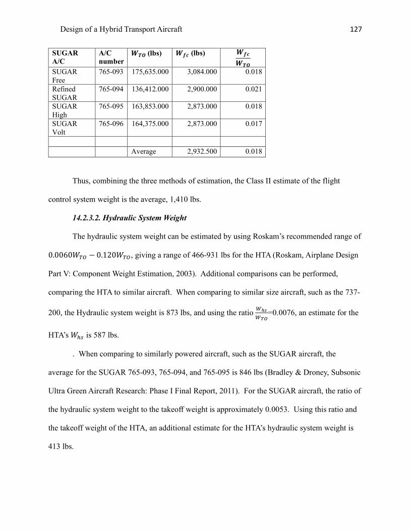
Design of a Hybrid Transport Aircraft 127
SUGAR A/C
A/C number
𝑾𝑻𝑶(lbs) 𝑾𝒇𝒄 (lbs) 𝑾𝒇𝒄
𝑾𝑻𝑶
SUGAR Free
765-093 175,635.000 3,084.000 0.018
Refined SUGAR
765-094 136,412.000 2,900.000 0.021
SUGAR High
765-095 163,853.000 2,873.000 0.018
SUGAR Volt
765-096 164,375.000 2,873.000 0.017
Average 2,932.500 0.018
Thus, combining the three methods of estimation, the Class II estimate of the flight
control system weight is the average, 1,410 lbs.
14.2.3.2. Hydraulic System Weight
The hydraulic system weight can be estimated by using Roskam’s recommended range of
0.0060𝑊ñò − 0.120𝑊ñò, giving a range of 466-931 lbs for the HTA (Roskam, Airplane Design
Part V: Component Weight Estimation, 2003). Additional comparisons can be performed,
comparing the HTA to similar aircraft. When comparing to similar size aircraft, such as the 737-
200, the Hydraulic system weight is 873 lbs, and using the ratio {UH{#$
=0.0076, an estimate for the
HTA’s 𝑊@9 is 587 lbs.
. When comparing to similarly powered aircraft, such as the SUGAR aircraft, the
average for the SUGAR 765-093, 765-094, and 765-095 is 846 lbs (Bradley & Droney, Subsonic
Ultra Green Aircraft Research: Phase I Final Report, 2011). For the SUGAR aircraft, the ratio of
the hydraulic system weight to the takeoff weight is approximately 0.0053. Using this ratio and
the takeoff weight of the HTA, an additional estimate for the HTA’s hydraulic system weight is
413 lbs.

Design of a Hybrid Transport Aircraft 128
Table 42. SUGAR Hydraulic System Weight Data
SUGAR A/C
A/C number
𝑾𝑻𝑶(lbs) 𝑾𝒉𝒔 (lbs) 𝑾𝒉𝒔
𝑾𝑻𝑶
SUGAR Free
765-093 175,635.000 894.000 0.005
Refined SUGAR
765-094 136,412.000 836.000 0.006
SUGAR High
765-095 163,853.000 827.000 0.005
SUGAR Volt
765-096 164,375.000 827.000 0.005
Average 846.000 0.005
Combining the estimates of 466 lbs, 931 lbs, 413 lbs, and 587 lbs, gives a Class II
estimate of 600 lbs for the weight of the hydraulic system.
14.2.3.3. Electrical System Weight
The Torenbeek Method to estimate the electrical system weight uses an equation that is a
function of the passenger cabin volume in cubic feet, 𝑉54L. This equation is as follows (Roskam,
Airplane Design Part V: Component Weight Estimation, 2003).
𝑊6$9 = 10.8Ç𝑉54LÉË.¥{1 − 0.018Ç𝑉54LÉ
Ë.u¨} (101)
The Torenbeek Method gives an estimate of 831 lbs.
The weight of the electrical system can be estimated from weights of similar electrical
systems, as well (Bradley & Droney, Subsonic Ultra Green Aircraft Research: Phase I Final
Report, 2011). The SUGAR aircraft electrical systems average 2362 lbs. Compared to their
takeoff weight, the ratio of electrical system weight to takeoff weight is 0.015. Using this ratio,
an estimate, from the SUGAR aircraft, for the electrical system weight of the HTA is 1152 lbs.
Using the 737-200 data from Roskam, the ratio of electrical system weight to takeoff weight is
0.009, and the resulting weight for the HTA’s electrical system is 716 lbs.

Design of a Hybrid Transport Aircraft 129
Table 43. SUGAR Electrical System Weight Data
SUGAR A/C
A/C number 𝑾𝑻𝑶(lbs) 𝑾𝒆𝒔 (lbs) 𝑾𝒆𝒔
𝑾𝑻𝑶
SUGAR Free
765-093 175,635.000 2,557.000 0.015
Refined SUGAR
765-094 136,412.000 2,297.000 0.017
SUGAR High
765-095 163,853.000 2,297.000 0.014
SUGAR Volt
765-096 164,375.000 2,297.000 0.014
Average 2,362.000 0.015
Averaging the resulting estimates from Torenbeek, SUGAR aircraft, and the 737-200, 𝑊69 = 900
lbs for the Class II estimate.
14.2.3.4. Instrumentation, Avionics, and Electronics Weight
The GD Method calculates the weight of the instruments as the sum of the flight
instruments, engine instruments, and other instruments as a function of the number of engines
and the number of pilots (Roskam, Airplane Design Part V: Component Weight Estimation,
2003).
𝑊" = 𝑁5"$ t15 + 0.032 ¬{#$tËËË
u+𝑁6 t5 + 0.006 ¬{#GtËËË
u+ 0.15 ¬{#$tËËË
+ 0.012𝑊ñò (102)
This method resulst in an estimate of 989 lbs.
The Torenbeek Method for jet transports is a function of the empty weight and the
maximum range in nautical miles (Roskam, Airplane Design Part V: Component Weight
Estimation, 2003).
𝑊"46 = 0.575𝑊6Ë.¨¨©𝑅Ë.N¨ (103)
The Torenbeek Method estimates 𝑊"46 to be 1,475 lbs.

Design of a Hybrid Transport Aircraft 130
These two methods can now be compared to the data gathered from the SUGAR aircraft
(Bradley & Droney, Subsonic Ultra Green Aircraft Research: Phase I Final Report, 2011). The
SUGAR aircraft, have a ratio of {�éJ{#$
=0.014, and therefore provide the HTA estimate for 𝑊"46 to
be 1,107 lbs. The Class II estimate for 𝑊"46 is 1,050 lbs.
Table 44. SUGAR Data for Instrumentation, Avionics, and Electronics Weight
SUGAR A/C
A/C number
𝑾𝑻𝑶(lbs) 𝑾𝒊𝒂𝒆 (lbs) 𝑾𝒊𝒂𝒆
𝑾𝑻𝑶
SUGAR Free
765-093 175,635.000 2,219.000 0.013
Refined SUGAR
765-094 136,412.000 2,277.000 0.017
SUGAR High
765-095 163,853.000 2,277.000 0.014
SUGAR Volt
765-096 164,375.000 2,277.000 0.014
Average 2,262.500 0.014
14.2.3.5. Air-Conditioning, Pressurization, and Anti- and Deicing Systems Weight
For pressurized commercial jet airplanes, the air-conditioning, pressurization system, and
the anti- and deicing systems weight, 𝑊45" can be estimated using the GD method. The GD
Method is a function of the passenger cabin volume in cubic feet, 𝑉54L , the number of crew
members, 𝑁BT, and the number of passengers, 𝑁54L. The equation below provides the estimate
(Roskam, Airplane Design Part V: Component Weight Estimation, 2003).
𝑊45" = 469 �~FéêÇr���rFéêÉtË,ËËË
�Ë.¤t§
(104)
The resulting GD Method estimate for 𝑊45" is 1,019 lbs.
The Torenbeek Method is a function of the length of the passenger cabin in feet, and is
summarized by the following equation (Roskam, Airplane Design Part V: Component Weight
Estimation, 2003).

Design of a Hybrid Transport Aircraft 131
𝑊45" = 6.75Ç𝑙54LÉt.N¦
(105)
The Torenbeek Method estimate is 1,496 lbs.
Compared to similar aircraft, such as the 737-200, with 𝑊45" = 1,416 lbs, and SUGAR
aircraft, which would give a ratio {éF�
{#$= 0.01, provides a low estimate of 792 lbs (Bradley &
Droney, Subsonic Ultra Green Aircraft Research: Phase I Final Report, 2011). For the Class II
estimate, the SUGAR aircraft data will be neglected, and 𝑊45"is estimated as the average of the
GD and Torenbeek Methods along with the 737-200 data and SUGAR A/C data as 1,181 lbs.
Table 45. SUGAR API Weight Data
SUGAR A/C
A/C number
𝑾𝑻𝑶(lbs) 𝑾𝒂𝒑𝒊 (lbs) 𝑾𝒂𝒑𝒊
𝑾𝑻𝑶
SUGAR Free
765-093 175,635.000 1,796.000 0.010
Refined SUGAR
765-094 136,412.000 1,549.000 0.011
SUGAR High
765-095 163,853.000 1,582.000 0.010
SUGAR Volt
765-096 164,375.000 1,582.000 0.010
Average 1,627.250 0.010
14.2.3.6. Oxygen System Weight
The weight of the oxygen system can also be estimated using both the GD Method and
Torenbeek Methods. The two equations, from Roskam are:
𝑊XL = 7Ç𝑁BT + 𝑁54LÉË.¥ËN
(106)
𝑊XL = 30 + 1.2𝑁54L (107)
As a result, the GD Method gives an estimate of 𝑊XL = 175𝑙𝑏𝑠, while the Torenbeek
Method gives an estimate of 𝑊XL = 145𝑙𝑏𝑠 for short flights above 25,000 ft, and 𝑊XL =

Design of a Hybrid Transport Aircraft 132
270𝑙𝑏𝑠 for extended flights overwater. Since the HTA is a short to medium range transport
aircraft, to determine a Class II estimate, 𝑊XL = 160 lbs.
14.2.3.7. Auxiliary Power Unit Weight
The Auliary Power Unit (APU) weight will be taken into account, since the jet transport
requires one. Although a specific APU has not been determined, the weight will be estimated
using Roskam’s estimate of the takeoff weight, along with comparisons for the 737-200 and the
SUGAR aircraft APU weights (Bradley & Droney, Subsonic Ultra Green Aircraft Research:
Phase I Final Report, 2011).
According to Roskam, 𝑊45> = 0.004𝑊ñò − 0.013𝑊ñò (Roskam, Airplane Design Part
V: Component Weight Estimation, 2003). This range is 310-1008 lbs, with an average of 660 lbs.
The SUGAR aircraft data gives an average APU weight of 1018.5 lbs, which is 0.6% of the
takeoff weight. Using this data gives a low estimate of 𝑊45> = 498 lbs. Taking the average of
these values gives a Class II estimate of 450 lbs.
Table 46. SUGAR APU Weight Data
SUGAR A/C
A/C number 𝑾𝑻𝑶(lbs) 𝑾𝒂𝒑𝒖 (lbs) 𝑾𝒂𝒑𝒖
𝑾𝑻𝑶
SUGAR Free
765-093 175,635 1,032 0.006
Refined SUGAR
765-094 136,412 1,014 0.007
SUGAR High
765-095 163,853 1,014 0.006
SUGAR Volt
765-096 164,375 1,014 0.006
Average 1,018.5 0.006
14.2.3.8. Furnishings Weight
Furnishings include cabin furniture and accessory items, like seats, insulation, trim
panels, sound-proofing, instrument panels, control stands, lighting, and wiring. Furnishings also

Design of a Hybrid Transport Aircraft 133
include galley provisions and the structure, the lavatory system, overhead luggage containers,
escape provisions, and fire-fighting equipment (Roskam, Airplane Design Part V: Component
Weight Estimation, 2003). The Torenbeek Method and GD Method will provide initial
estimates, with the SUGAR data and the 737-200 data providing additional support for the Class
II Estimate.
The GD Method and Torenbeek Method provide the following equations, respectively to
calculate 𝑊=>T .
𝑊=>T = 55𝑁=3B + 32𝑁54L + 15𝑁BB + 𝑘$48Ç𝑁54LÉt.uu + 𝑘R>=Ç𝑁54LÉ
t.tN + 109 trFéê(t���)tËË
uË.¨Ë¨
+ 0.771¬{#$tËËË
(108)
𝑊=>T = 0.211(𝑊ñò −𝑊ó)Ë.§t (109)
These two equations yield 𝑊=>T = 3,918 and 5,655 lbs, respectively. The 737-200 aircraft gives
an estimate of 𝑊=>T = 4,463lbs, and using the ratio provided by the Sugar aircraft data, below,
𝑊=>T = 4,651 lbs.
Table 47. SUGAR Aircraft Furnishings Weight Data
SUGAR A/C
A/C number 𝑾𝑻𝑶(lbs) 𝑾𝒇𝒖𝒓 (lbs) 𝑾𝒇𝒖𝒓
𝑾𝑻𝑶
SUGAR Free
765-093 175,635.000 10,866.000 0.062
Refined SUGAR
765-094 136,412.000 9,115.000 0.067
SUGAR High
765-095 163,853.000 9,115.000 0.056
SUGAR Volt
765-096 164,375.000 9,115.000 0.055
Average 9,552.750 0.060
Nikolai also provides a method to determine the weight of the furnishings. It is the sum
of the crew seats, passenger seats, miscellaneous furniture, and the cabin windows. The
equations that provide these, respectively are as follows (Nikolai, 1984).

Design of a Hybrid Transport Aircraft 134
𝑊B9 = 34.5(𝑁BT)𝑞Ë.N¨ (110)
𝑊59 = 32.03(𝑁54L) (111)
𝑊E = 0.771(𝑊ñò ∗ 10Úu) (112)
𝑊B[ = 109.33Ç𝑁54L(1 + 𝑃B) ∗ 10ÚNÉË.¨Ë¨
(113)
𝑊B9,𝑁_𝑐𝑟, 𝑞,𝑊59,𝑁54L,𝑊E,𝑊B[,𝑃B are the weight of the crew’s seats, the number of crew, the
dynamic pressure, weight of the passenger’s seats, number of passengers, weight of
miscellaneous furnishings, weight of the cabin windows, and th ultimate fabin pressure in Psi,
respectively. Using these equations, results in the following weights: 𝑊B9 = 318𝑙𝑏𝑠,𝑊59 =
3,075𝑙𝑏𝑠,𝑊E = 60𝑙𝑏𝑠, 𝑎𝑛𝑑𝑊B[ = 539lbs, with a total of 3991 lbs.
The Class II weight estimate for furnishings weight will be 3,991 lbs.
14.2.3.9. Baggage and Cargo Handling Equipment Weight
According to Roskam, the baggage and cargo containers’ weight can be estimated using
𝑊RB = 1.6 ∗ 𝑙𝑏𝑠/𝑓𝑡u (114)
There will be 3 containers at 80 ft3 each, for a total of 240 ft3, which gives the total weight to be
384 lbs, as the Class II estimate for 𝑊RB.
14.2.3.10. Operational Items Weight
The operational items include food, water, drinks, china, and lavatory supplies. Using the
SUGAR aircraft database, below, the Class II estimate of the HTA’s operational items weight
will be calculated (Bradley & Droney, Subsonic Ultra Green Aircraft Research: Phase I Final
Report, 2011). Assuming the operational items weight as 4.6% the takeoff weight, the HTA’s
estimate for operational items weight from SUGAR A/C data is 𝑊X59 = 3,540 lbs.

Design of a Hybrid Transport Aircraft 135
Table 48. SUGAR Data for Operational Items Weight
SUGAR A/C
A/C number
𝑾𝑻𝑶(lbs) 𝑾𝒐𝒑𝒔 (lbs) 𝑾𝒐𝒑𝒔
𝑾𝑻𝑶
SUGAR Free
765-093 175,635.000 7,342.000 0.042
Refined SUGAR
765-094 136,412.000 7,207.000 0.053
SUGAR High
765-095 163,853.000 7,207.000 0.044
SUGAR Volt
765-096 164,375.000 7,207.000 0.044
Average 7,240.750 0.046
According to Nikolai’s Fundamental’s of Aircraft Design,
𝑊$48 = 1.11 ∗ 𝑁54Lt.uu (115)
𝑊=XX3 = 𝐾Ü�ó ∗ 𝑁54Lt.tN (116)
where 𝑊$48 is the weight of the lavatories and water provisions, 𝑊=XX3 is the weight of the food
provisions, and 𝐾Ü�ó = 5.68𝑜𝑟1.02 for long range flights and short range flights, respectively
(Nikolai, 1984). Combining these weights for 96 passengers give an estimate for the operational
weight of 650 lbs. This is significantly less than the data from the SUGAR A/C. Differences
include the number of passengers, and the length of the flight.
The calculated value of 650 lbs will be used as the estimate for the Class II operational
weight.
14.2.3.11. Weight of Paint
Roskam provides the following equation to estimate the weight of paint for a well painted
airplane to be:
𝑊5Y = 0.003𝑊ñò − 0.006𝑊ñò (117)

Design of a Hybrid Transport Aircraft 136
This gives a range of 233-466 lbs and an average of 349 lbs. The 737-700 uses approximately
350 lbs of paint (Hansen, n.d.). The Class II estimate will use an equivalent ratio of paint equal
to 260 lbs.
14.2.3.12. Fixed Equipment Weight Summary
Table 49. Fixed Equipment Weight Summary
Component GD Method (lbs)
Torenbeek Method (lbs)
Roskam Method (lbs)
Estimate from 737 A/C (lbs)
Estimate from SUGAR A/C (lbs)
Estimate from Nikolai (lbs)
Class II Estimate (lbs)
Flight Control System
1633.4 1164.4 ---------- ---------- 1432 -------- 1,410
Hydraulic System
--------- ------------ 466-931 873 413 -------- 600
Electrical System
---------- 831 --------- 716 1,152 -------- 900
Instrumetation, Avionics, and Electronics
989 1,475 --------- ---------- 1,107 -------- 1,050
Air-Conditioning, Pressurization, Anti and De-icing
1,019 1,496 -------- 1,416 793 -------- 1,181
Oxygen System
175 145-208 ------ ------- ----------- -------- 160
APU ---------- --------- 310-1008
------------ 498 -------- 450
Furnishings 3,919 5,655 --------- 4,463 4,652 3,991 3,991 Baggage and Cargo
--------- ---------- 384 ----------- ------------- -------- 384
Operational Items
--------- ---------- -----------
----------- 3,540 650 650
Paint 233-466 350 ------- 260 TOTAL 11,036
14.2.4. Empty Weight Discussion
The empty weight is the sum of the structural weight, powerplant weight, and fixed
equipment weight. 𝑊6 = 𝑊9YT>BY + 𝑊5[T +𝑊=6% . Combining the totals from each of these

Design of a Hybrid Transport Aircraft 137
sections gives a total estimate of 52,439 lbs for the empty weight. Note that the nacelle weights
were accounted for in the powerplant weight calculations, and the structural nacelle weight
estimate will be neglected, since the manufacturer’s data is available for the powerplant.
For the HTA, which uses fuel only in stages 1-4, and is battery powered for the
remaining stages, the Class I estimate for the empty weight is 48,379 lbs. This difference of
4,060 lbs is fairly close to the Class I estimate, and gives a 7.7% difference.
The Class II weight sizing will need to be iterated if the weight savings criteria that
follows does not provide a convergence. The weight savings criteria involve manufacturing the
fuselage from composites, which would save 15% of the weight, manufacturing parts of the wing
and fuselage under low stress from composites, which would save about 5%, and using a
quadruplex digital flight control system and fly-by-wire as opposed to mechanical flight controls,
which would save 15%, and replacing the primary wing and fuselage structure with lithium
aluminum, which would give a 6% weight savings (Roskam, Airplane Design Part II:
Preliminary Configuration Design and Integration of the Propulsion System, 2011). Thus, the
empennage weight could be reduced by 394 lbs; the wing and fuselage low-stress composite
replacement could be reduced by 713 lbs; the flight controls system could be reduced by 212 lbs;
and the lithium aluminum would reduce the wing and fuselage structure by 857 lbs. Thus, the
estimated empty weight has been lowered to 50,263 lbs, now only a 3.7% difference.
Considering the percent difference is small, and the Class I weight sizing will continue to be
used.
14.3. Component Centers of Gravity
The c.g. locations for the structural components, powerplant, and fixed equipment
components will be presented using Roskam’s guidelines. The table below illustrates the c.g.

Design of a Hybrid Transport Aircraft 138
location of the structural components, powerplant, and fixed equipment (Roskam, Airplane
Design Part V: Component Weight Estimation, 2003).
Using the revised Class II weights and the c.g. locations for both the x and z direction
gives the following weights summary.
Table 50. Class II Weights and CG locations
No. Type of Component
Wi (lbs) xi (in.) Wixi (in lbs) yi (in.) Wiyi (in lbs)
zi (in.) Wizi (in lbs)
1 Fuselage Group
7,130 641 4,570,330 0 0 248 1,768,240
2 Wing Group
5,568 680 3,786,240 0 0 350 1,948,800
3 Empennage Group
2,233 1190 2,657,270 0 0 300 669,900
4 Engine Group
21,778 590 12,849,020 0 0 140 3,048,920
5a Landing Gear Group:Nose Gear
500 390 195,000 0 0 130 65,000
5b Landing Gear Group: Main Gear
2224 710 1,579,040 0 0 130 289,120
6 Fixed Equipment Group
10,824 680 7,360,320 0 0 200 2,164,800
7 Trapped Fuel and Oil
34.4 690 23,736 0 0 215 7,396
8 Crew 700 300 210,000 0 0 240 168,000 9 Fuel 3,440 690 2,373,600 0 0 430 1,479,200
10 Batteries 12,000 733 8,796,000 0 0 120 1,440,000 11 Passengers 16,800 680 11,424,000 0 0 200 3,360,000 12 Luggage 3,000 680 2,040,000 0 0 200 600,000
The x c.g. location is located at 55.9 ft, and the z c.g. location is located at 16.4 ft based on the
equations from Roskam (Roskam, Airplane Design Part V: Component Weight Estimation,
2003).

Design of a Hybrid Transport Aircraft 139
𝑥B7 = ∑ {�L�{
#"Ät (118)
𝑧B7 = ∑ {�D�{
#"Ät (119)
If any of the components are moved, then the c.g. location moves according to the following
equation (Roskam, Airplane Design Part V: Component Weight Estimation, 2003).
∆𝑥B7 =∆L�({�)∑ {�I��Á
(120)
The most likely movement could be the batteries, but since they are suspended below the wings,
they do not have a wide range of movement available.
The c.g. excursion plot, based on the Class II data, is illustrated in the figure below. The
plot illustrates that the most forward c.g. location is at 57.33 ft and the most aft c.g. location is at
72.11 ft. This was plotted by varying the number of passengers, luggage, and fuel. The
conditions included a fully loaded aircraft, an aircraft with half passenger and full fuel, all
passengers and half the luggage, zero passengers and full luggage, no passengers and no cargo,
zero fuel, passengers only, and cargo only.
Figure 90. Class II cg excursion diagram
0
10000
20000
30000
40000
50000
60000
70000
80000
90000
100000
650 700 750 800 850 900 950
Wei
ght (
lbs)
F.S. (in)
c.g. Excursion Diagram

Design of a Hybrid Transport Aircraft 140
14.4. Airplane Inertias
To estimate the moments and products of inertia for the HTA, the weights from the Class
II sizing and the c.g. locations in feet will be used. The engine group will be one weight and c.g.
location, and will therefore be a ‘lumped mass’ assumption. This is also true for the passengers
and fuel systems. The structural components will also be assumed to have uniform mass
distributions. The following table summarizes the moments and products of inertia.
Table 51. Moments and products of Inertia
𝐼LL 𝐼ææ 𝐼DD 𝐼Læ 𝐼æD 𝐼DD
111,166.12 314,123.14 202,957.02 0 0 -52,406.14
The table was computed using the following equations (Roskam, Airplane Design Part V:
Component Weight Estimation, 2003).
𝐼LL = ∑ 𝑚" tÇ𝑦" − 𝑦B7ÉN+ Ç𝑧" − 𝑧B7É
Nu#
"Ät (121)
𝐼ææ = ∑ 𝑚" tÇ𝑧" − 𝑧B7ÉN+ Ç𝑥" − 𝑥B7É
Nu#
"Ät (122)
𝐼DD = ∑ 𝑚" tÇ𝑥" − 𝑥B7ÉN+ Ç𝑦" − 𝑦B7É
Nu#
"Ät (123)
𝐼Læ = ∑ 𝑚"�(𝑥" − 𝑥B7)(𝑦" − 𝑦B7)�#"Ät (124)
𝐼æD = ∑ 𝑚"�(𝑦" − 𝑦)(𝑧" − 𝑧B7)�#"Ät (125)
𝐼DL = ∑ 𝑚"�(𝑧" − 𝑧B7)(𝑥" − 𝑥B7)�#"Ät (126)
15. Cost Analysis
The life cycle cost consists of the research and development costs, production and
construction costos, operations and maintenance costs, and retirement and disposal costs. For
typical aircraft, the operating costs composes nearly 94% of the life cycle cost (Ploetner,

Design of a Hybrid Transport Aircraft 141
Schmidt, Baranowski, Isikveren, & Hornung, 2013). Thus, the preliminary cost analysis for the
HTA will consider the operating cost (Roskam, Airplane Design Part II: Preliminary
Configuration Design and Integration of the Propulsion System, 2011).
In order to estimate the program operating cost, 𝐶X59, direct operating cost, DOC, and
indirect operating cost, IOC, mission data will be reviewed. These calculations will require the
block distance, 𝑅R$, block time, 𝑇R$, block speed, 𝑉R$ , and annual utilization in block hours,
𝑈4##]^ . The block distance can be considered the door to door distance. This distance will be the
1,720 nm established for the HTA. The block time is the door to door time from the departure
gate to the parking spot. The block time is calculated through the following equations (Roskam,
Airplane Design Part VIII: Airplane Cost Estimation: Design, Development, Manufacturing, and
Operating, 2015).
𝑇R$ = 𝑇7E + 𝑇B$ + 𝑇BT + 𝑇36 (127)
𝑇7E = 0.51(10)Ú©(𝑊ñò) + 0.125 (128)
𝑇BT = (1.06𝑅R$ − 𝑅B$ − 𝑅36 + 𝑅E4#)/𝑉�T (129)
𝑅B$ = (𝑉B$)(𝑇B$) (130)
𝑅E4# = (𝑉E4#)(𝑇E4#) (131)
𝑇E4# = 0.25(10Ú©)𝑊ñò + 0.0625 (132)
The times consisting of the time spent on ground maneuvers, 𝑇7E, such as leaving the gate,
taxiing to the runway, time on the takeoff run, on the landing ground run, and taxiing to the
destination, time spent in climb, 𝑇B$, time spent in cruise, 𝑇BT, and time spent in descent, 𝑇36. The
ground maneuver time dependso n the takeoff weight, and the time for cruise depends on the
block distance, 𝑅R$, distance for climb, 𝑅B$, distance for descent, 𝑅36 , maneuvering distance,
𝑅E4#, and the cruise velocity, 𝑉BT. The distance for climb depends on the climb velocity and the
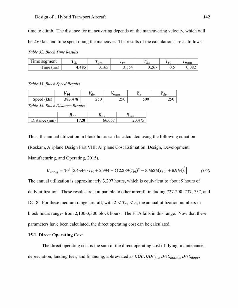
Design of a Hybrid Transport Aircraft 142
time to climb. The distance for maneuvering depends on the maneuvering velocity, which will
be 250 kts, and time spent doing the maneuver. The results of the calculations are as follows:
Table 52. Block Time Results
Time segment 𝑻𝒃𝒍 𝑇7E 𝑇BT 𝑇36 𝑇B$ 𝑇E4# Time (hrs) 4.485 0.165 3.554 0.267 0.5 0.082
Table 53. Block Speed Results
𝑽𝒃𝒍 𝑉36 𝑉E4# 𝑉BT 𝑉36 Speed (kts) 383.478 250 250 500 250
Table 54. Block Distance Results
𝑹𝒃𝒍 𝑅36 𝑅E4# Distance (nm) 1720 66.667 20.475
Thus, the annual utilization in block hours can be calculated using the following equation
(Roskam, Airplane Design Part VIII: Airplane Cost Estimation: Design, Development,
Manufacturing, and Operating, 2015).
𝑈4##]^ = 10u Ù3.4546 ∙ 𝑇R$ + 2.994 − (12.289(𝑇R$)N − 5.6626(𝑇R$) + 8.964)Á�Ý (133)
The annual utilization is approximately 3,297 hours, which is equivalent to about 9 hours of
daily utilization. These results are comparable to other aircraft, including 727-200, 737, 757, and
DC-8. For these medium range aircraft, with 2 < 𝑇R$ < 5, the annual utilization numbers in
block hours ranges from 2,100-3,300 block hours. The HTA falls in this range. Now that these
parameters have been calculated, the direct operating cost can be calculated.
15.1. Direct Operating Cost
The direct operating cost is the sum of the direct operating cost of flying, maintenance,
depreciation, landing fees, and financing, abbreviated as 𝐷𝑂𝐶,𝐷𝑂𝐶=$Y, 𝐷𝑂𝐶E4"#Y, 𝐷𝑂𝐶365T,

Design of a Hybrid Transport Aircraft 143
𝐷𝑂𝐶$#T, and 𝐷𝑂𝐶="# , respectively. Each of these direct operating costs will be measured in
USD/nm. Each of these will be calculated and summed to find the total direct operating cost.
15.1.1. Direct Operating Cost of Flying
The direct operating cost of flying consists of the sum of the cost of the crew, 𝐶BT6[, cost
of the fuel and oil, cost of the batteries, and cost of the airframe insurance.
15.1.1.1. Cost of the Crew
The cost of the crew depends on the number of crew members, 𝑛BC,the type of crew
member, with 𝑛BÁbeing the captain and 𝑛B� being the co-pilot, the factor, 𝑘µ, which accounts for
vacation pay, cost of training, crew insurance and premiums, and payroll tax, the block speed,
𝑉R$ , the annual salaries of the crew members, 𝑆𝐴𝐿µ, the number of flight hours per year for a
crew member, 𝐴𝐻µ, and the travel expense factor, 𝑇𝐸𝐹µ.
CBT6[ = ∑ m𝑛BC tt�ëC~]^
u ª�ÛzCÛ�C
« + ¬ñ�óC~]^
¦µ"Ät (134)
All the of the costs are for 2018. They have been scaled using the cost escalation factor,
CEF, which is
𝐶𝐸𝐹æ64T = 6.008930 + 0.10280(𝑦𝑒𝑎𝑟 − 2014) (135)
There will be two crew members for the HTA, a captain and co-pilot. The salaries of each
fo the respective crew members will be assumed to be $158,686 and $102,679. Flight crew will
be assumed to fly an average of 800 flight hours per year. The travel expense factor for each of
the crew is 13.06 per block hour. Thus, the total cost of the crew is 1.14 USD/nm.
15.1.1.2. Cost of the Fuel and Oil
The cost of fuel and oil, 𝐶5X$, depends on the mission fuel weight, the price of the fuel,
FP, and the density of the fuel, FD.

Design of a Hybrid Transport Aircraft 144
𝐶5X$ = 1.05 ¬{<]^�]^
¬ó�ów (136)
The current fuel price is $2.20 per gallon (Jet Fuel Daily Price, 2018). The fuel density is 6.74
lbs/gallon (Roskam, Airplane Design Part VIII: Airplane Cost Estimation: Design, Development,
Manufacturing, and Operating, 2015). Using a mass fuel fraction of 0.955696, the weight of the
fuel, and thus the weight of the block fuel is 3,438 lbs. The total cost of fuel and oil in USD per
nautical mile is 0.69 USD/nm.
15.1.1.3. Cost of the Batteries
To determine the direct operating cost fo the batteries, 𝐷𝑂𝐶R4Y, measured in USD/nm, the
following assumptions will be made. The flight will require 35,314 kWh for the flight.
Generally, the cost per charge per kWh is $0.0085. Thus the rate in USD/nm for the batteries
charge is 0.17 USD/nm. Note that the initial cost of the battery is not included in this.
15.1.1.4. Summary of Direct Operating Cost of Flying
The direct operating cost of flying, 𝐷𝑂𝐶=$Y, can be calculated using the following
equation (Roskam, Airplane Design Part VII: Determination of Stability, Control and
Performance Characteristics: FAR and Military Requirements, 2006).
𝐷𝑂𝐶=$Y = 𝐶BT6[ + 𝐶5X$ + 𝐶"#9 + 𝐶R4Y (137)
Since the cost of insurance is 2% of the direct operating cost, the direct operating cost of flying if
a function of the direct operating cost. DOC¡)1 = 2.10 + 0.02(𝐷𝑂𝐶) USD/nm.
15.1.2. Direct Operating Cost of Maintenance
The direct operating cost of maintenance is calculated using the following equation, from
Roskam. The direct operating cost of maintenance is the sum of the labor cost of the airframe
and systems maintenance, labor cost of the engine maintenance, cost of maintenance materials
for the airframe and system, cost of maintenance materials for the engines, and applied

Design of a Hybrid Transport Aircraft 145
maintenance burden, all measured in USD/nm. The following equations summarize the
calculations necessary to determine the direct operating cost of maintenance (Roskam, Airplane
Design Part VIII: Airplane Cost Estimation: Design, Development, Manufacturing, and
Operating, 2015).
𝐷𝑂𝐶E4"#Y = 𝐶$4R/45 + 𝐶$4R/6#7 + 𝐶E4Y/45 + 𝐶E4Y/6#7 + 𝐶4ER (138)
𝐶$4R/45 = 1.03(𝑀𝐻𝑅E45]^)(𝑅$éF)/(𝑉R$) (139)
𝐶$4R/6#7 = 1.03(1.3)𝑁6(𝑀𝐻𝑅E6#7]^)(𝑅$JIK)/(𝑉R$) (140)
𝐶E4Y/45 = 1.03Ç𝐶E4Y/45R$@TÉ𝑉R$ (141)
𝐶E4Y/6#7 = 1.03 ∗ 1.3 ∗ 𝑁6 ∗ 𝐶E4Y/6#7R$@T/𝑉R$ (142)
𝐶4ER = 1.03 tÇ𝑓4ER/$4RÉ ÙÇ𝑀𝐻𝑅E45]^É ¬𝑅$éF + (𝑁6)Ç𝑀𝐻𝑅6#7]^É ¬𝑅$JIKÝ +
Ç𝑓4ER/$4Rɨ𝐶E4Y/45R$@T + (𝑁6)𝐶E4Y/6#7R$@T©u /𝑉R$ (143)
The maintenance labor cost for the airframe and system depends on the number of
maintenance manhours per blockhour for airframe systems, which is 6.35 hours, the weight of
the airframe, which is 26,601 lbs, and the airplane maintenance labor rate per manhour, of 16
USd/nm. These inputs produce 𝐶$4R/45 = 0.3142USD/nm.
The cost of the maintenance labor for the engines depends on the number of engines, the
number of engine maintenance hours per engine, which will be assumed to be 5 hours, the hourly
labor rate for engine maintenance, at $18.40, and the block speed of 383.5 kts. This produces
𝐶$4R/6#7 = 0.64 USD/nm.
The cost of maintenance materials for the airframe and systems, other than the engines,
depends on the airframe price, and the cost of the maintenance materials per blockhour, at 100
USD/nm. Thus, C0*1/*- = 0.27 USD/nm.
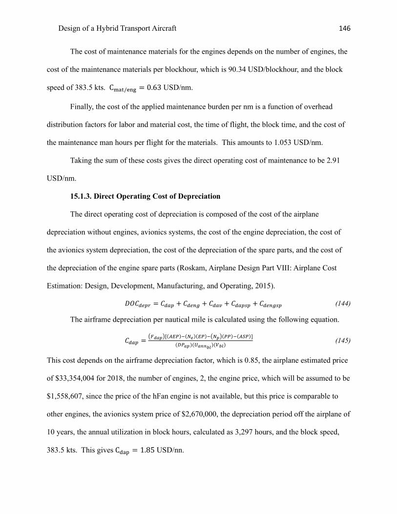
Design of a Hybrid Transport Aircraft 146
The cost of maintenance materials for the engines depends on the number of engines, the
cost of the maintenance materials per blockhour, which is 90.34 USD/blockhour, and the block
speed of 383.5 kts. C0*1/.&/ = 0.63 USD/nm.
Finally, the cost of the applied maintenance burden per nm is a function of overhead
distribution factors for labor and material cost, the time of flight, the block time, and the cost of
the maintenance man hours per flight for the materials. This amounts to 1.053 USD/nm.
Taking the sum of these costs gives the direct operating cost of maintenance to be 2.91
USD/nm.
15.1.3. Direct Operating Cost of Depreciation
The direct operating cost of depreciation is composed of the cost of the airplane
depreciation without engines, avionics systems, the cost of the engine depreciation, the cost of
the avionics system depreciation, the cost of the depreciation of the spare parts, and the cost of
the depreciation of the engine spare parts (Roskam, Airplane Design Part VIII: Airplane Cost
Estimation: Design, Development, Manufacturing, and Operating, 2015).
𝐷𝑂𝐶365T = 𝐶345 + 𝐶36#7 + 𝐶348 + 𝐶34595 + 𝐶36#795 (144)
The airframe depreciation per nautical mile is calculated using the following equation.
𝐶345 =ÇóÆéFÉ[(Û��)Ú(rJ)(��)ÚÇrFÉ(��)Ú(Û��)]
(w�éF)(�éII]^)(~]^) (145)
This cost depends on the airframe depreciation factor, which is 0.85, the airplane estimated price
of $33,354,004 for 2018, the number of engines, 2, the engine price, which will be assumed to be
$1,558,607, since the price of the hFan engine is not available, but this price is comparable to
other engines, the avionics system price of $2,670,000, the depreciation period off the airplane of
10 years, the annual utilization in block hours, calculated as 3,297 hours, and the block speed,
383.5 kts. This gives C£*- = 1.85 USD/nn.

Design of a Hybrid Transport Aircraft 147
The cost of engine depreciation per nautical mile is calculated using:
𝐶36#7 =ÇóÆJIKÉrJ(��)
(w�JIK)(�éII]^)(~]^) (146)
This equation depends on the engine depreciation factor of 0.85, the engine depreciation period
of 7 years, which may change when using the new hybrid engines, and other previously
established factors of engine price, annual utilization in block hours, and block speed. The result
is that C£.&/ = 0.299USD/nm.
The cost of the depreciation of the avionics sytem in USD per nautical mile is calculated
using:
𝐶348 =(óÆéV)Û��
(w�éV)(�éII]^)(~]^) (147)
Thus, C£*« = 0.42 USD/nm with an avionics system depreciation factor of 1 and the
depreciation time to be 5 years.
The cost of the depreciation of airplane spare parts in USD/nm is calculated using:
𝐶34595 =ÇóÆéFHFÉÇóéFHFÉÇÛ��Ú(rJ)(��)É
(w�éFHF)(�éII]^)(~]^) (148)
Thus C£*-�- is a function of the airplane spare parts depreciation factor of 0.85, the airplane
spare parts factor of 1, the airplane spare parts depreciation period of 10 years, and other
previously calculated values. C£*-�- = 0.20 USD/nm.
The cost of the depreciation of engine spare parts is given by:
𝐶34595 =(�ÆJIKHF)ÇóJIKHFÉ(r_6)(��)(����ó)
(w�JIKHF)(�éII]^)(~]^) (149)
C£*-�- = 0.23 USD/nm, and is based on the engine spare parts depreiciation factor of 0.85, the
engine spare parts factor of 0.5, the engine spare parts price factor of 1.50, the depreciation
period for the engine spare parts, which is 7 years, and the block speed and annual utilization.

Design of a Hybrid Transport Aircraft 148
Summarizing, DOC£.-� = C£*- + C£.&/ + C£*« + C£*-�- + C£.&/�- = 1.85 + 0.299 +
0.42 + 0.20 + 0.23 = 3.01 USD/nm.
15.1.4. Direct Operating Cost of Landing Fees, Navigation Fees, and Registry Taxes
The direct operating cost of landing fees, navigation fees, and registry taxes is given by
the following equations (Roskam, Airplane Design Part VIII: Airplane Cost Estimation: Design,
Development, Manufacturing, and Operating, 2015).
𝐷𝑂𝐶$#T = 𝐶$= + 𝐶#= + 𝐶TY (150)
𝐶$= = (𝐶45$=)/(𝑉R$𝑇R$) (151)
𝐶#= = (𝐶45#=)/(𝑉R$𝑇R$) (152)
𝐶TY = 𝑓TY(𝐷𝑂𝐶) (153)
The landing fee cost is 0.09 USD/nm, with the airplane landing fee per landing being
155.21 USD/nm. The cost of navigation fee will be assumed to be $0 USD/nm as the plane will
not fly internationally. The cost of financing will be assumed to be 0.58 USD/nm, and the cost of
registry taes is 0.01 USD/nm. Thus, the resulting sum is 0.099 USD/nm.
15.1.5. Direct Operating Cost of Financing
The direct operatinc cost of financing, 𝐷𝑂𝐶="# is 7% of the DOC. Thus, this amounts to
approximately 0.34 USD/nm.
15.1.5. Direct Operating Cost Discussion
The direct operating cost, totals 8.45 USD/nm. The following chart illustrates the
breakdown of the DOC for a jet transport aircraft.

Design of a Hybrid Transport Aircraft 149
Figure 91. DOC for a Jet Transport
Based off of the calculations for the direct operating cost for the HTA, the figures below
illustrates the breakdown of the DOC for both the HTA and a fuel version of the HTA. There is a
significant decrease in fuel usage, but higher maintenance due to the batteries. Additionally,
there is an increase in the depreciation with batteries due to the life cycles.
Figure 92.HTA DOC with batteries and fuel
36%
29%
30%
1%4%
DOC SUMMARYFlight MaintenanceDepreciation Landing FeesFinance
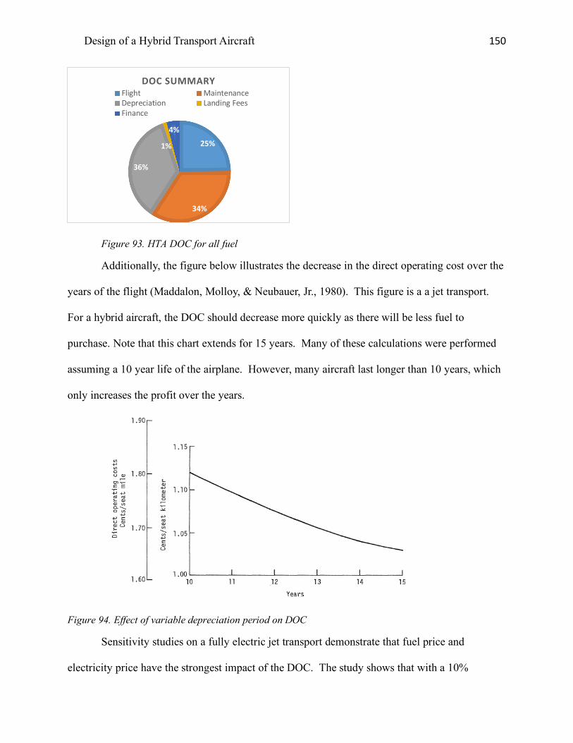
Design of a Hybrid Transport Aircraft 150
Figure 93. HTA DOC for all fuel
Additionally, the figure below illustrates the decrease in the direct operating cost over the
years of the flight (Maddalon, Molloy, & Neubauer, Jr., 1980). This figure is a a jet transport.
For a hybrid aircraft, the DOC should decrease more quickly as there will be less fuel to
purchase. Note that this chart extends for 15 years. Many of these calculations were performed
assuming a 10 year life of the airplane. However, many aircraft last longer than 10 years, which
only increases the profit over the years.
Figure 94. Effect of variable depreciation period on DOC
Sensitivity studies on a fully electric jet transport demonstrate that fuel price and
electricity price have the strongest impact of the DOC. The study shows that with a 10%
25%
34%
36%
1%
4%
DOC SUMMARYFlight MaintenanceDepreciation Landing FeesFinance

Design of a Hybrid Transport Aircraft 151
increase in fuel costs, there is a 3% increase in DOC. Additionally, a reduction in the number of
cycles of battery use, less than the typical 2000 cycles, combined with battery installation costs
also produces higher DOCs (Ploetner, Schmidt, Baranowski, Isikveren, & Hornung, 2013).
15.2. Indirect Operating Cost
The indirect operating cost, 𝐼𝑂𝐶,is composed of the indirect operating cost for passenger
services, maintaining depreciating ground equipment and facilitiesm airplane and traffic
servicing, promotions sales, and entertainment, and general administrative expenses. Its units are
in USD/nm. The costs for these services can be estimated through the equation:
𝐼𝑂𝐶 = 𝐹"XB(𝐷0𝐶) (154)
𝐹"XB is the factor extrapolated from the 737 data from Roskam. This factor is 0.5. Thus, the
indirect operating cost is 4.14 USD/nm.
15.3. Program Operating Cost
The program operating cost depends on the indirect program operating costs, the direct
program operating costs, and the number of aircraft acquired. Due to the fact that operating costs
vary between customers, the program operating costs depends on the number of customers. For
the purposes of these calculations, 1,200 aircraft will be assumed to be in acquisition (Sales,
2018). As of January 1, 2018, Boeing has orders for more than 4,300 737- MAX aircraft. Since
the HTA has similar mission specifications, a high volume will be assumed for acquisition. Then
the program operating cost can be estimated using the following equations (Roskam, Airplane
Design Part VIII: Airplane Cost Estimation: Design, Development, Manufacturing, and
Operating, 2015).
𝐶X59 = ∑ ÙÇ𝐶X59Æ��É"Ç𝑁4B%É" + Ç𝐶X59�IÆÉ"Ç𝑁4B%É"Ý"Ä#"Ät (155)
Ç𝐶X59Æ��É" = (𝐷𝑂𝐶)"Ç𝑅R$4##É"Ç𝑁æTÉ" (156)
Design of a Hybrid Transport Aircraft 152
Ç𝐶X59�IÆÉ" = (𝐼𝑂𝐶)"Ç𝑅R$4##É"Ç𝑁æTÉ" (157)
Assuming the aircraft are in use for 10 years, the operating cost is $190,835,543,254.38. The
early design has a significant impact on the ultimate cost of the aircraft. In the future, trade
studies can be performed on the number of years in service and the number of aircraft acquired
per year to determine the effect on the operating cost.
15.3. Hybrid Power Cost Analysis
Although the price of jet fuel fluctuates per gallon, the general trend illustrates an
increase in fuel costs and an increase in the number of general aviation aircraft, as discussed in
the introduction. The price of electricity to recharge the batteries is significantly cheaper than jet
fuel and has the added benefit of drastically reducing carbon dioxide and other harmful
emittants. Electricity costs approximately 8.5 cents per kilowatt hour. For a fully-fuel powered
version of the HTA, which requires 17,888 lbs or 2,670 gallons of jet fuel, this would reduce the
cost of the total fuel per flight from $5,874 to $1,129.
15.3.1. Sample Battery Specifications
Although battery technology is not yet at its peak in power, companies are selling
advanced lithium ion batteries for aviation power. True Blue Power is one such company.
For aviation, True Blue has a 46 amp hour battery, which at an output voltage of 26.4
Volts, and weight of approximately 23.4 kg, gives approximately 51.7 Wh/kg of energy. The low
specific energy density would result in more batteries and higher weight, further illustrating the
need for increased battery energy density. However, with the promise of better battery
technology and the capabilities of lithium ion batteries, these batteries may provide future
capabilities.

Design of a Hybrid Transport Aircraft 153
This battery has a life expectancy of 8 years with a 2 year maintenance interval. It
weighs 51.7 lbs and has superior performance at extreme temperatures, including -40ºF to 158ºF
and at pressures up to 35 Psi. Its dimensions are 10.9 in by 10.5 in by 10.1 in, making it easily
fit in small spaces and configure with other batteries (True Blue Power, 2018). Each battery
costs approximately $16,400 (True Blue Power, 2018). Though the batteries may initially be
expensive, this one time cost for the life of the aircraft will drastically decreasethe cost to power
the aircraft over time.
16. Conclusion
The preliminary design of the narrow-body, short to medium range hybrid transport
vehicle demonstrates the feasibility of a hybrid powered aircraft fueld by both lithium ion
batteries and jet fuel. Through a series of Class I estimates, including configuration design,
weight sizing and sensitivities, determination of performance constraints, fuselage and cockpit
design, wing design, empennage design, landing gear design, weight and balance analysis,
stability and control analysis, and drag polar estimation, and Class II estimates of the V-n
maneuver diagram, and weight and balance, and cost analysis, the early design calculations
carefully layout the conversion of a jet aircraft to a hybrid powered aircraft.
This vehicle provides an environmentally friendly form of flight, reducing emissions and
dependence on oil. As the number of general aviation aircraft increase and FAA standards call
for reduced emissions, designing aircraft with less dependence on oil and fuel is becoming
necessary. With battery technology developing, a hybrid aircraft is the perfect transition to
greener aircraft for the near future.
Compared to the Boeing 737-100 model, the HTA has comparable weights, with the
possibility of a lower takeoff weight. Additionally, with the research behind the SUGAR aircraft,

Design of a Hybrid Transport Aircraft 154
the availability of hybrid engines would make the transition of power between fuel and
electricity much more simple to integrate.
In regards to future work, the battery technology will continue to develop, and, as a result
the weight may decrease and the specific energy densities may increase. Additionally, more
studies could be performed on the benefits of using fuel and battery power during different
phases of the flight. Trade studies could show the advantages and disadvantages of each power
source during the phase of flight. The direct operating cost, although preliminary, demonstrates
that the batteries, as a power source, are competitive from a cost perspective.
Overall, the hybrid transport aircraft demonstrates strong potential as a preliminary
design to meet FAA standards, reduce emissions, and utilize future battery technology to pave
the way toward new-age transport jets.

Design of a Hybrid Transport Aircraft 155
References
Airbus Commerial Aircraft. (n.d.). Retrieved July 5, 2017, from
http://www.aircraft.airbus.com/aircraftfamilies/passengeraircraft/a320family/a320neo/
Aircraft Technical Data and Specifications: Boeing 737-100/200. (2017). Retrieved from
Airliners: http://www.airliners.net/aircraft-data/boeing-737-100200/91
An Encyclopedia of the History of Technology. (2002). In I. McNeil (Ed.). Routledge.
Boeing Commercial Airplanes. (2013). 737 Airplane Characteristics for Airport Planning.
Bradley, M. K., & Droney, C. K. (2011). Subsonic Ultra Green Aircraft Research: Phase I Final
Report. Huntington Beach: Boeing Research and Technology.
Bradley, M. K., & Droney, C. K. (2015). Subsonic Ultra Green Aircraft Research: Phase II-
Volume II- Hybrid Electric Design Exploration. NASA. Huntington Beach: Boeing
Research and Technology.
Bradley, M. K., & Droney, K. C. (2011). Subsonic Ultra Green Aircraft Research: Phase I Final
Report. Langley Research Center. Hampton: National Aeronautics and Space
Administration.
Bradley, M. K., Droney, C. K., & Allen, T. J. (2015). Subsonic Ultra Green Aircraft Research:
Phase II Volume I Truss Braced Wing Design Exploration. NASA.
Brady, C. (1999). Detailed Technical Data. Retrieved from The 737 Technical Site:
http://www.b737.org.uk/techspecsdetailed.htm
Canadair Regional Jet. (2016). Canadair Regional Jet Airport Planning Manual. Toronto:
Bombardier Inc.
Crawford, B. (2009). Flightlab Ground School. Flight Emergency and Advanced Maneuvers
Training Inc.

Design of a Hybrid Transport Aircraft 156
Creative Aviation Photography. (2017). Retrieved from Airplane Pictures: http://www.airplane-
pictures.net
Daggett, D. L., Hendricks, R. C., Rainer, W., & Corporan, E. (2008). Alternate Fuels for Use in
Commercial Aircraft. National Aeronautics and Space Administration, Glenn Research
Center, Cleveland.
Davis, S. C., Williams, S. E., & Boundy, R. G. (2016). Transportation Energy Data Book (35
ed.). Oak Ridge, Tennessee: Oak Ridge National Laboratory.
Farhadi, M., & Mohammed, O. (2016). Energy Storage Technologies for High-Powered
Applications. IEEE Transaction on Industry Applications, 52(3), 1953-1961.
Federal Aviation Administration. (2015). Aviation Emissions, Impacts, and Mitigation: A Primer.
Office of Environment and Energy.
Fuel Price Analysis. (2017). Retrieved from IATA:
http://www.iata.org/publications/economics/fuel-monitor/Pages/price-analysis.aspx
Hansen, D. (n.d.). Airframe Design. Retrieved from The Boeing Company:
http://www.boeing.com/commercial/aeromagazine/aero_05/textonly/fo01txt.html
Hepperle, M. (n.d.). Electric Flight- Potential and Limitations. NATO OTAN.
Jane's All the World's Aircraft. (2013). IHS Markit.
Jet Fuel Daily Price. (2018, May 14). Retrieved from index mundi:
https://www.indexmundi.com/commodities/?commodity=jet-fuel
Maddalon, D. V., Molloy, J. K., & Neubauer, Jr., M. J. (1980). NASA Technical Memorandum
80196: Computer Programs for Estimating Civil Aircraft Economics. Hampton: NASA
Langley Research Center.

Design of a Hybrid Transport Aircraft 157
Mason, W. H. (2006). Aerodynamic Configuration Design Options. In Configuration
Aerodynamics.
Matsushita, T., Yabuta, K., Tsujikawa, T., Matsushima, T., Arakawa, M., & Kurita, K. (2008).
Construction of Three-Dimensional Thermal Simulation Model of Lithium Ion Secondary
Battery. IEEE, 1-6.
Moore, R. H., Shook, M., Beyersdorf, A., Corr, C., Hendon, S., Knighton, W. B., . . . Anderson,
B. E. (2015). Influence of Jet Fuel Composition on Aircraft Engine Emissions: A
Synthesis of Aerosol Emissions Data from the NASA APEX, AAFEX, and ACCESS
Missions. Energy & Fuels, 29, 2591-2600.
NASA. (2014, January 24). In Future Aircraft Designs We "Truss". (L. Gipson, Editor) Retrieved
2017, from https://www.nasa.gov/aero/boeing_sugar_wind_tunnel.html
Nikolai, L. M. (1984). Fundamentals of Aircraft Design. San Jose: METS, Inc.
Obert, E. (2009). Aerodynamic Design of Transport Aircraft. Delft University of Technology .
Ploetner, K. O., Schmidt, M., Baranowski, D., Isikveren, A. T., & Hornung, M. (2013).
Operating Cost Estimation for Electric-Powered Transport Aircraft. American Institute of
Aeronautics and Astronautics.
Riboldi, C., & Gualdoni, F. (2016). An integrated approach to the preliminary weight sizing of
small aircraft. Aerospace Science and Technology, 58, 134-149.
Roskam, J. (2003). Airplane Design Part V: Component Weight Estimation. Lawrence:
DARcorporation.
Roskam, J. (2006). Airplane Design Part VII: Determination of Stability, Control and
Performance Characteristics: FAR and Military Requirements. Lawrence :
DARcorporation.
Design of a Hybrid Transport Aircraft 158
Roskam, J. (2011). Airplane Design Part 3: Layout Design of Cockpit, Fuselage, Wing, and
Empennage: Cutaways and Inboard Profiles. Lawrence: DARcorporation.
Roskam, J. (2011). Airplane Design Part II: Preliminary Configuration Design and Integration
of the Propulsion System. Lawrence: DARcorporation .
Roskam, J. (2011). Airplane Design Part III: Layout Design of Cockpit, Fuselage, Wing, and
Empennage: Cutaways and Inboard Profiles. Lawrence: DARcorporation.
Roskam, J. (2015). Airplane Design Part VIII: Airplane Cost Estimation: Design, Development,
Manufacturing, and Operating. Lawrence: DARcorporation.
Roskam, J. (2017). Airplane Design Part 1: Preliminary Sizing of Airplanes. DARcorporation.
Rudolph, P. C. (1996). High-Lift Systems on Commercial Subsonic Airliners. Moffett Field:
NASA Ames Research Center.
Sales. (2018, Feb. 10). Retrieved from The Boeing 737 Technical Site:
http://www.b737.org.uk/sales.htm
Tariq, M., Maswood, A. I., Gajanayake, C. J., & Gupta, A. K. (2017). Aircraft batteries: current
trend towards more electric aircraft. The Institute of Engineering and Technology, 7(2),
93-103.
Thauvin, J., Barraud, G., Roboam, X., Sareni, B., Budinger, M., & Leray, D. (2016). Hybrid
Propulsion for Regional Aircraft: a Comparative Analysis Based on Energy Efficiency.
IEEE.
True Blue Power. (2018). TB46. Retrieved from True Blue Power:
https://www.truebluepowerusa.com/aviation-products/advanced-lithium-ion-
batteries/tb46/
Ullman, D. (n.d.). The Electric Powered Aircraft: Technical Challenges.

Design of a Hybrid Transport Aircraft 159
Xue, N. (2014). Design and Optimization of Lithium-Ion Batteries For Electric Vehicle
Applications .
Zayat, K. A., Dray, L., & Schafer, A. (2017). A First Order Analysis of Direct Operating Costs of
Battery Electric Aircraft. Antwerp: Engineering and Physical Sciences Research Council.