design of self-restriction hydrostatic thrust spherical

International Journal of Mechanical Engineering and Applications 2019; 7(4): 111-122

http://www.sciencepublishinggroup.com/j/ijmea

doi: 10.11648/j.ijmea.20190704.14

ISSN: 2330-023X (Print); ISSN: 2330-0248 (Online)

Design of Self-restriction Hydrostatic Thrust Spherical Bearing (Fitted Type)

Ahmad Waguih Yacout Elescandarany

Mechanical Department, Faculty of Engineering, Alexandria University, Alexandria, Egypt

Email address:

To cite this article: Ahmad Waguih Yacout Elescandarany. Design of Self-restriction Hydrostatic Thrust Spherical Bearing (Fitted Type). International Journal

of Mechanical Engineering and Applications. Vol. 7, No. 4, 2019, pp. 111-122. doi: 10.11648/j.ijmea.20190704.14

Received: August 14, 2019; Accepted: September 4, 2019; Published: September 20, 2019

Abstract: This is the last part of the series studying the fitted hydrostatic thrust spherical bearing. It handles an

unconventional design of this type of bearings. The conception of this design is to break the rules controlling the bearing

restrictions, where it is believed that without restrictors no hydrostatic bearing could be got (axiom). The paper focused the

effort to derive a general characteristic equation that can control the design in turn the bearing performance and behavior. This

general characteristic equation, through its simple form, gives the designer the ability to get a comprehensive conception about

his problem and widely opens the door in front of him to design a conventional or unconventional bearing whatever the

bearing purpose. The effective parameters; needed to be known for designing the bearing; were concentrated into three items;

the rotor speed, the seat dimensions and the lubricant properties. The characteristic equation shows that the seat radius and the

inlet angle play the major role in determining the supply pressure, in turn the load carrying capacity. The inertia, the recess

angle and the lubricant viscosity have the major effect on determining the bearing stiffness in case of the partial hemispherical

seats while in case of the hemispherical seats the stiffness has slightly been affected. The design shows that the bearings with

hemispherical seats have extremely low stiffness, practically zero stiffness and very high temperature rise, which make this

bearing configuration invalid to be self restriction bearing; while the bearings with partial hemispherical seats have a very wide

stiffness range allowing the designer to control and design the bearing with the stiffness needed for any purpose (from zero

stiffness to extremely high stiffness). The lubricant temperature rises about three degrees centigrade which practically means

that the bearing operates at constant temperature.

Keywords: Hydrostatic Bearings, Spherical Bearings Design, Surface Roughness, Inertia, Viscosity Effects,

Self Compensation

1. Introduction

The previous researches offered plenty of the traditional

studies and designs of the hydrostatic thrust spherical bearing

with restrictors or with self-compensation.

Ahmad W. Yacout [1-4] studied the fitted type, with and

without recess, of the hydrostatic thrust spherical bearing

with capillaries and orifices restrictors finding the effects of

the inertia, surface roughness and lubricant fluid viscosity on

the beating performance and offering an optimal design of

this bearing.

Kane N. R. et al [5] offered a design of a hydrostatic rotary

bearing with angled surface self-compensation consisting of

five precisely machined parts provided with a sealing system.

It is concluded that the novel hydrostatic bearing is

potentially useful for applications that require very high

rotational precision and stiffness in a low profile package.

Xiaobo Z. et al [6] investigated the influence of design

parameters on the static performance of a designed self-

compensating hydrostatic rotary bearing where the results

showed that the optimum designed resistance ratio is 1; the

initial clearance ratio should be small, and the inner

resistance ratio should be large.

Yuan K. et al [7] studied a hydrostatic bearing with double-

action variable compensation of membrane-type restrictors

(DAMR) and self-compensation (SC) where it is concluded

that the critical (ddc) dimensionless deformation coefficient

value of DAMR which corresponds to infinite stiffness is (2/3)

and the static characteristics of self-compensation (SC) are

always same as that of constant restrictors.

112 Ahmad Waguih Yacout Elescandarany: Design of Self-restriction Hydrostatic Thrust Spherical Bearing (Fitted Type)

Xu C. and Jiang S. [8] conducted a comparative study of

the static behavior between the self-compensation hydrostatic

spherical hinge and the hydrostatic spherical hinge with

orifice restrictor where the results showed that the self-

compensation hydrostatic spherical hinge has an advantage in

the static behavior over the hydrostatic spherical hinge with

orifice restrictor, including a much larger load capacity, a

smaller flow rate, and a smaller power loss.

Khaksea P. G. et al [9] offered a comparative study for the

performance of a non-recessed hole-entry Hybrid/

Hydrostatic conical bearing compensated with capillary and

orifice Restrictors where it is concluded that, in general,

orifice compensated non-recess conical journal bearing

showed higher performance characteristics as compared to

the counterpart bearing for the applied radial load.

Zhifeng Li et al [10] offered a fruitful review of

hydrostatic bearing system where the articles about

hydrostatic bearings since 1990 were collected in this review.

Researching status was evaluated in two aspects: basic theory

and typical application. Basic theory contains equations and

analysis methods which include analytic, numerical, and

experimental methods. Typical applications were based on

rectangular oil pad, circular oil pad, and journal bearings.

Moreover, the review focused on the analysis of the relevant

model, solution, and optimization and summarized the

hotspots and development directions.

Alexander S. [11-12] discussed and compared between

bearings with restrictors and others of self compensation

using different lubricants (oil & water) where the study

proved the priority of the self compensation type numerating

its advantages and concluding that it makes the system far

less sensitive to contamination especially if water is used, it

provides greater stiffness and load capacity and it makes the

system insensitive to manufacturing tolerances. Besides the

bearings are self-tuning where the stiffness automatically

optimizes itself for the bearing as soon as it is turned on (no

manual tuning of capillary or orifice size is required) and the

bearing is not significantly affected by large gap variations

caused by manufacturing tolerances which make the bearing

suitable for use with water or water based coolant as a

bearing lubricant.

Z. Y. Dong et al [13] obtained the relationships of

worktable displacement, load capacity, and static stiffness by

using flow continuity equations of a self-compensated

hydrostatic bearing. The results revealed that the appropriate

range of design parameters for self-compensated hydrostatic

bearing can obtain the maximum stiffness.

Mohit Agarwal [14] studied the stiffness of an opposed

pad hydrostatic bearing showing that the performance of a

hydrostatic bearing can be improved over a certain range of

load capacity if the design parameters of the restrictor set-up

are properly chosen where the design restriction ratio should

be chosen differently for lower and higher loading conditions

for high static stiffness.

Antony Wong [15] presented, through the master thesis, a

design and manufacturing method for a new surface self

compensating hydrostatic bearing where a lumped resistance

model was used to analyze the performance of the bearing

and provide guidance on laying out the bearing features;

concluding the results of the model indicate the design is

extremely robust.

The present design of hydrostatic thrust spherical bearing

is utilizing a new untraditional technique, self-restriction,

which helps the designer to get rid of the compensators

allowing very low design complexity.

2. Mathematics

The mathematical bearing expressions are listed in the

appendix.

2.1. Bearing General Characteristic Equation

2.1.1. Bearing with Orifice Restrictor

From Yacout [1-4]

1

2

2

4

[ ]3

8

0.6 Re 15

5 10

so

d oo

d o

o

oo

oi

pq K

C dK

C

d x m

dm

d

πρ

−

=

=

= → >

>

=

(1)

3

9

s

qQ

e p

µπ

= (2)

1

22

Re [ ]3

o so

d pρµ

= (3)

From 1, 2:

26 2 4 4(1.215 ) ( )o io

s

e Q m dp

µρ

= (4)

From 3, 4:

3 3 30.9( )Re

o ioo

e Q m d= (5)

2.1.2. Bearing with Capillary Tube Restrictor

4

( )3

, ( )128

20 ( )

( )

Re 2000 ( )

cap

s

ccap

c

cc

io

cc

io

c

Kq p

dK a

l

ln b

d

fm c

d

e

µπ

=

=

= ≥

=

≤

(6)

International Journal of Mechanical Engineering and Applications 2019; 7(4): 111-122 113

From equations (2, 6):

3 3 33( )2560

c ioe Q m d= (7)

2.1.3. The Relation Between the Two Restrictors

From equating equations (5, 7):

Re 768 & Re 2000o c= =

Hence, the general characteristic governing equation for

this type of bearings is:

3 3 3

3 3 3

0.9( )768

3( )2560

o io

c io

e Q m d or

e Q m d

=

= (8)

Put:

c om m m= =

3 3 3 3(1.172 10 ) ioe Q x m d−= (9)

Equation (9) is the general characteristic governing

equation for this type of bearings.

2.2. Restrictor-less Bearing

Equating (m) with the unity, equation (8 or 9) becomes:

3 3

3 3 3

3( )2560

(1.172 10 )

io

io

e Q d or

e Q x d−

=

= (10)

3. Restrictor-less Bearing Design

Generally, Equation (9) could be used to design a bearing

with or without restrictors as needed and equation (10) could

directly be used for designing the restrictor-less (self

restriction) bearing.

3.1. Determining the Supply Pressure

From equations (4, 9):

22 6 43

( ) (1.215 1) ( )2560

io ios

d x dp

µρ

=

26

2(0.884736 10 )( )

2 sin

s

io

io i

p xd

d R

µρ

φ

=

=

26

2 2(0.221184 10 )( )

sins

i

p xR

µρ φ

= (11)

3.2. Determining the Seat Inlet Angle ( iφ )

The angle ( iφ ) could be determined as:

2 2

2 2

9

80

9

80

2

s

s

RS

P

RP

N

ρ

ρ

π

Ω=

Ω=

Ω =

Relating with equation (11), then:

1

700sin ( )

700sin ( )

i

i

S

N a

S

N a

µφρ

µφρ

−

=

= (12)

To get the best benefit from the inertia in the design, the

speed parameter (S = 1)

3.3. Determining the Design Eccentricity

From equations (13, 15 and 16) the quantity (3e Q ) could

be calculated at different values of (e) at the design speed

parameter (S). Drawing this quantity against (e), the design

eccentricity (e) which satisfies equation (10) could be

graphically determined in turn the design (Q).

3.4. Determining the Load Carrying Capacity

Getting the design (e), the inlet and exit bearing angles

( &i eθ θ ) could be calculated as in Yacout [1-4], the

dimensionless load carrying capacity (W) could be calculated

from equation (17).

3.5. Determining the Total Losses (Pt)

From equations (18-21) the total bearing losses could be

calculated.

3.6. Temperature Rise and Distribution

From equations (22-23) the temperature rise could be

theoretically and numerically calculated.

3.7. Determining the Bearing Stiffness

The theoretical or numerical stiffness calculations of this type

of bearings are extremely tedious due to the crescent shape of

the film thickness and the complicated relation between the load

and the film thickness. However, the stiffness will be handled in

some details based on the film thickness direction.

3.7.1. Axial Bearing Stiffness ( aλ )

Putting into consideration that the film thickness in the

thrust direction is:

2cosah e θ=

The stiffness could be calculated numerically in the thrust

direction following the same procedures as found in the

appendix to be:

1( )

l

a al lλ λ

==∑


3.7.2. Transversal Bearing Stiffness ( tλ )

The film thickness in the transversal direction is:

cos sinth e θ θ=

Hence:

1( )

l

t tl lλ λ

==∑

3.7.3. Radial Bearing Stiffness ( rλ )

The film thickness in the transversal direction is:

cosrh e θ=

Hence:

1( )

l

r rl lλ λ

==∑

3.7.4. Internal Bearing Stiffness ( θλ )

The detailed theoretical derivation is in the appendix

where:

The internal localized stiffness is:

22( ) ( )cos

R p

eθ

πλ θ=

And the mean internal stiffness is:

( )e

i

θθ θ θ θ

λ λ=

=∑

4. Design Example

It is required to design a high speed bearing with (50 mm)

radius, maximum rotor speed (N =500 r. p. s) and intended

load (L = 20 KN).

5. Design Procedures

5.1. Selections

5.1.1. Lubricant Fluid Properties

(µ = 0.086 N.s /m2, Kv = 0.5, ρ = 867 N.s

2/m

4, Cv =1880

J/Kg. c0)

5.1.2. Geometrical Dimensions

2eφ ηπ= , ( )i tobecalculatedφ r eYφ φ= , 0.81η = , 0.3Y =

5.1.3. Surface Roughness Specifications

(ξ = 0.05)

5.2. Design Calculations

5.2.1. Determining the Seat Inlet Angle ( iφ )

From equation (12):

2

1

sin (700 0.086 867 500 0.05 ) 0.014

sin (0.014)

0.8

2 sin

1.4

i

i

oi

io i

io

x x x x

d R

d mm

φ π

φ

φφ

−

= =

=

===

5.2.2. Determining the Supply Pressure ( sP)

From equation (11):

26

2 2

6 2

2 2

6 2

(0.221184 10 )( )sin

0.221184 10 0.068( )

867 0.05 0.014

2.41 10 /

s

i

s

s

P xR

x xP

x x

P x N m

µρ φ

=

=

=

5.2.3. Determining the Eccentricity (e)

The quantity (3e Q ) could be easily calculated at different

values of (e), drawn against (e) and the design eccentricity

which satisfies equation (10) could be graphically determined

in turn the design (Q).

From figure 1-a:

3 -12e 3.2023x10

168.2

0.6725

Q

e m

Q

µ=

==

Figure 1. Partial with recess.

5.2.4. Determining the Load Capacity (w)

From equation (17) the load could be calculated to be:

20.718w KN=

Hence, the load factor of safety ( sf ) is:

3

34

20.718 10

20 10

1.0359

s

s

w xf

L x

f

= =

=


So, this load should not be exceeded.

5.2.5. Determining the Flow Rate (q)

3

12 63

-5 3

-5 3

( )

6

(3. 120230 ) (2 / 3) (2.4141x10 )/

6 0.068

3.9684x10

3.9684x10 (3600 10 ) /

142.864 /

se Q pq

x x x xq m s

x

q m s

q x l hr

q l hr

π βµ

π −

=

=

=

==

5.2.6. Determining the Pump Power ( pP)

From equation (19):

-5 6

.

(3.9684x10 ) (2.41 10 )

95.77 . /

p s

p

p

p q p

P x x

P N m s

=

=

=

5.2.7. Determining the Temperature Rise (∆T)

The temperature rise could be theoretically calculated as:

-5

95.77

867 1880 3.9684x(10 )

1.48

p

v

o

PT

q C

Tx x

T C

ρ∆ =

∆ =

∆ =

Or numerically by equation (22) and from the temperature

distribution figure 1:

2.86 oT C∆ =

5.2.8. Determining the Stiffness

Applying equations (24-29) the localized stiffness and the

mean stiffness could be determined.

a) Determining the radial Stiffness ( Rλ )

From figure 2-a & table 1

110 /R N mλ µ=

b) Determining the axial stiffness ( Aλ )

From figure 2-b & table 1

188.4 /A N mλ µ=

c) Determining the transversal stiffness ( Tλ )

From figure 2-c & table 1

347 /T N mλ µ=

d) Determining the internal stiffness ( θλ )

From figure 2-d & table 1

132 /N mθλ µ=

Figure 2. Partial with recess.

Figure 3. Partial without recess.

Figure 4. Partial without recess.


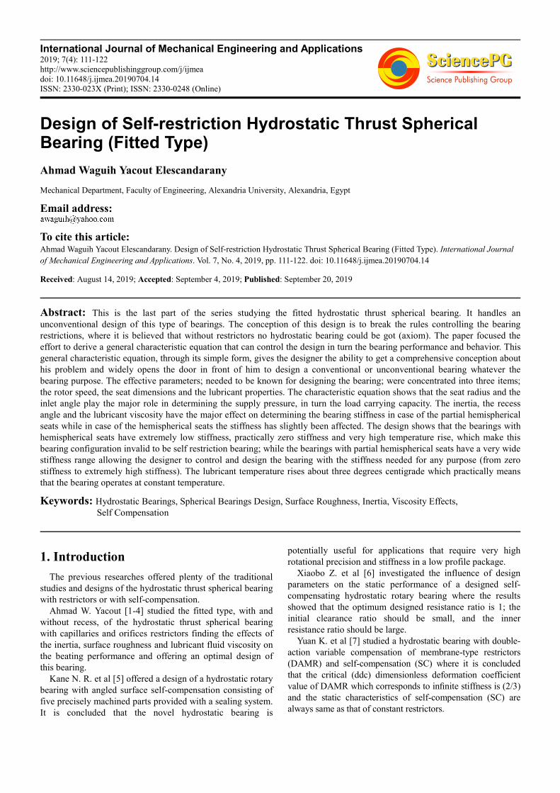
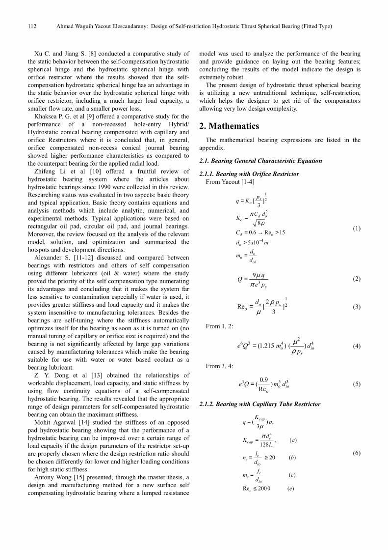
Figure 5. Hemi with recess.

Figure 6. Hemi with recess.

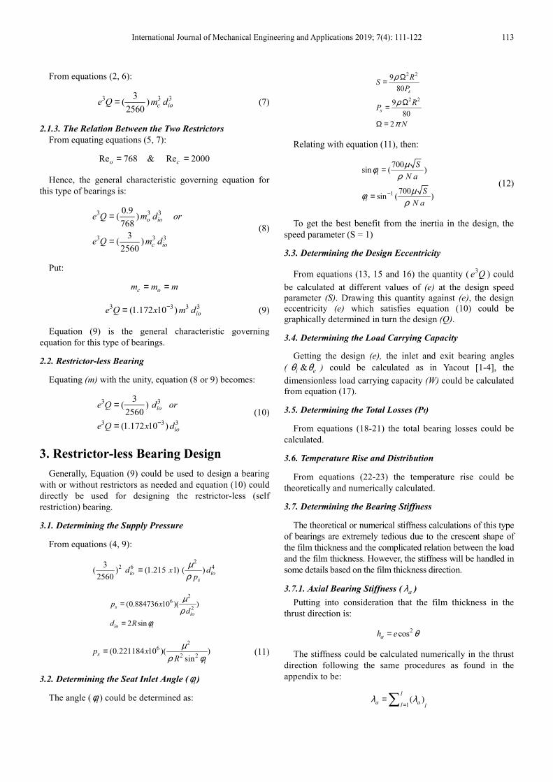
Figure 7. Hemi without recess.

Figure 8. Hemi without recess.

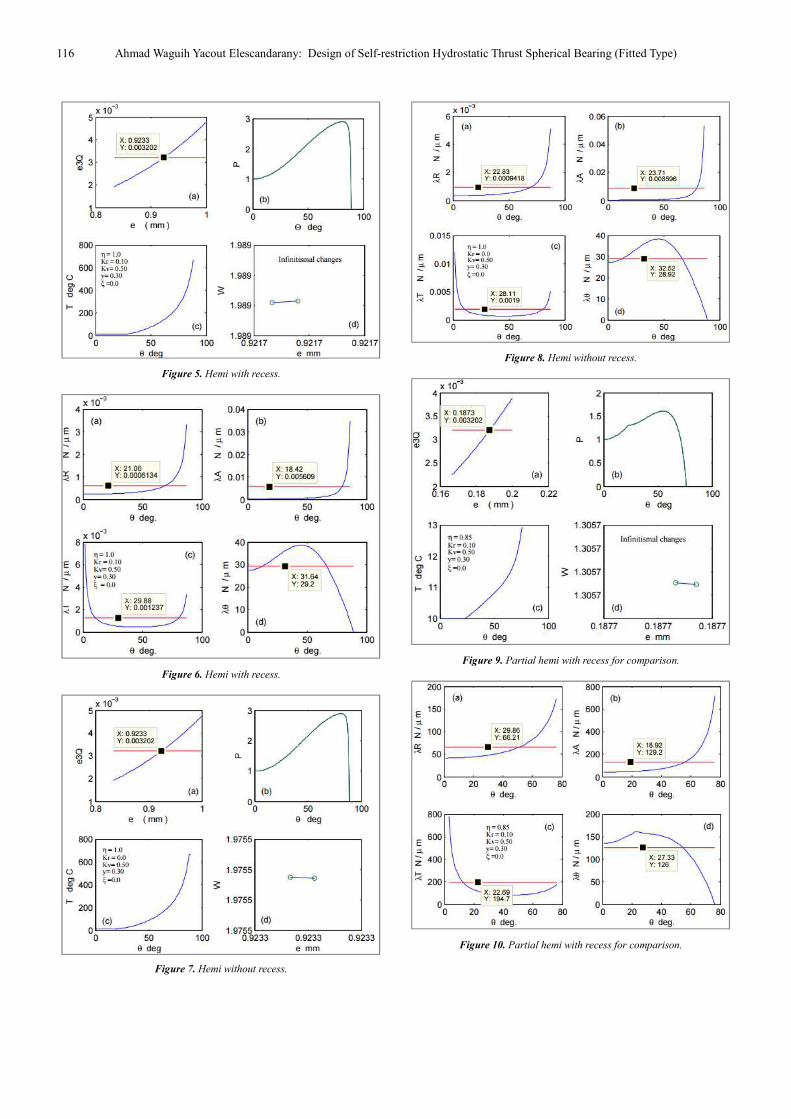
Figure 9. Partial hemi with recess for comparison.

Figure 10. Partial hemi with recess for comparison.


Table 1. Collecting the bearing data.

Bearing

Parameters

Without recess With recess

H. S P.H. S H. S P. H. S

ξ 0.05 0.05 0.05 0.05

η 1 0.81 1 0.81

ϕi (deg) 0.8 0.8 0.8 0.8

ϕr ≈ 0 0 27 21.9

ϕe ≈ 90 72.9 90 72.9

∆ (mm) 0 0 5 5

dio ≈ 1.4 1.4 1.4 1.4

R ≈ 50 50 50 50

Aw (cm)2 79 79 79 79

Load (KN) 20 20 20 20

N (r. p. s) 500 500 500 500

ρ (N.s2 /m4) 867 867 867 867

µ (N.s /m2) 0.068 0.068 0.068 0.068

Cv (J/ Kg.c) 1880 1880 1880 1880

θi (degree) 0.79 0.8 0.79 0.8

θr ≈ 0 0 26.5 21.8

θe ≈ 89 72.7 89 72.7

β (dim-less) 2/3 2/3 2/3 2/3

Ps (MN / m2) 2.41 2.41 2.41 2.41

e (mm) 0.9233 0.203 0.9217 0.1682

he ( µm) 17 60.5 17 50

Ke (dim-less) 1/54.2 1/246 1/60 1/300

S ≈ 1 1 1 1

w (KN) 38.45 5.29 38.7 20.718

fs = (w/L) 1.87 0.264 1.88 1.0359

Q (dim-less) 0.0041 0.3802 0.0041 0.6725

q (m / hr) 0.1429 0.1429 0.1429 0.1429

Pp (N. m/s) 95.43 95.62 95 95.77

λA (N / µm) 0.009 12.8 0.0056 188.4

λR ≈ 0.0009 8.5 0.0006 110

λT ≈ 0.002 23.7 0.0012 347

λθ ≈ 29 25 29.2 132

∆Tn (deg. c) 656 3.33 649 2.86

∆Tth (deg. c) 1.48 1.48 1.47 1.48

6. Bearing Configuration Checking

The selected configuration is checked to find out the effect

of different parameters ( , , ,r vkη θ ξ ) on the design.

6.1. Effect of (η )

The seat arc length is lengthened to be (0.85) of the

hemispherical one to be put in comparison with the designed

one.

6.2. Effect of (y)

The recess arc length is extended to be (0.4) of seat arc one

through increasing recess angle ( rθ ).

6.3. Effect of ( vk )

The lubricant is treated as a constant fluid viscosity i.e.

( 0vk = ).

6.4. Effect of (ξ )

The bearing surface is treated as an utmost allowed

roughened conformal surface in the hydrodynamic regime

i.e. ( 1ξ = ).

7. Results

As previously stated, it is the last part of a study handling

this type of bearings. A new technique is used to design an

unconventional bearing. A general characteristic equation is

derived to express this bearing function and test its design

validation. A bearing is designed as an example to test the

ability of the new technique, through the general

characteristic equation, to offer a self-restriction bearing i.e.

restrictor-less bearing. Ten figures (1-10) and two tables (1-

2) express the calculations results.

8. Discussion

Because of the novelty, the discussion may contain some

necessary details needed to reveal the author opinion and

options.

8.1. Bearing Design Technique

The design technique is merely based on unifying the

dominant bearing parameters, the supply pressure, the

lubricant flow rate and seat inlet orifice diameter ( . ,s ioP q d )

through the derived general characteristic equation to ease

and simplify the bearing selection (regardless of it is with or

without restrictor) depending only on its configuration that

succeeds to meet the required application demands.

8.2. General Characteristic Equation

This new equation is derived through relating the capillary

and orifice restrictors of the bearing and equating the two

ratios ( cm and om ) to get equation (9). The equation expresses

the characteristic of this type of bearing in general. Despite

of its simplicity the equation relates the eccentricity (e), the

lubricant flow rate, the central pressure ratio, central and

supply pressures ( , ,i sp p β ); through (Q); the bearing

inlet orifice diameter and the restrictor diameter; through (m).

Hence, it could be truly considered as the General

Characteristic Bearing Equation, it controls the bearing

parameters and never act the bearing outside its domination.

Equating the ratio (m) with unity makes the restrictor

parameter (m) disappear yielding equation (10). Now, this

equation does not point to or contain a restrictor, which

theoretically means that it expresses a restrictor-less

bearing. The physical meaning of disappearing (m) is that

the inlet bearing orifice does not only act as a flow

passage but also as an orifice restrictor. The previous

studies handling the subject of designing untraditional

bearings depend on the bearing outlet passage to act as a

restrictor where the bearings are called as self

compensation [5-10].

So, the author prefers to call the present bearing,


mathematically, as a restrictor-less bearing or, physically as a

self-restriction bearing.

For the aforementioned reasons the author chooses the

self-restriction bearing as a name of this new bearing.

8.3. The Eccentricity

The odd figures (1-7 a) and Table 1 show the

determination of the eccentricity values for the different

baring configurations.

8.4. Load Carrying Capacity

Table 1 shows that the partial un-recessed bearing

configuration has failed to carry the required load.

8.5. The Temperature Rise and Distribution

The temperature rise is theoretically and numerically

calculated.

8.5.1. The Theoretical Solution

Equation (22) is applied to calculate the temperature rise

but it is impotent to help the designer finding the feature of

this rise.

8.5.2. The Numerical Solution

While Equation (22) is unable to give the designer an idea

about the temperature rise feature equation (23) can do.

8.5.3. The Calculation Results

The odd figures (1-7 c) express the temperature variation

along the lubricant passage which got through the numerical

solution of equation (23). Figures (5, 7 c) show that the

temperature has gone up to 650 C which makes the

hemispherical bearing configuration with or without recess

unsuitable for the design required conditions in spite of its

stiffness which will be discussed in the next item to assure its

invalidity.

8.6. The Bearing Stiffness (λ)

The stiffness in the author previous studies hasn't been

handled in details.

8.6.1. The Numerical Solution

This numerical solution depends on disturbing the bearing

eccentricity (e) through changing it by an infinitesimal

quantity resulting in changing the radial thickness ( rh ), the

pressure (p) and in turn the load capacity (w) by infinitesimal

quantities. Hence, the stiffness is calculated as the ratio

between the infinitesimal changes of (w) and ( rh ). Because

the radial thickness varies depending on its position as a

function of (θ) the stiffness ( rλ ) also will be local depending

on the ( rh ) position. The mean value of these local stiffness

points is the mean stiffness.

The thickness ( rh ) is analyzed in the axial ( ah ) and

transverse ( th ) directions where the stiffness is based on the

infinitesimal changes in these directions to be ( aλ ) and ( tλ )

equation (25-27).

8.6.2. The Theoretical Solution

A simple mathematical method is used to calculate the

stiffness mathematically. The integration of the load capacity

is differentiated relatively to the thickness to avoid the

complications in the integration process and then the

complications of re-differentiating the integrated load

equation. It is seen from equation (28) that the stiffness is

directly proportional to the pressure (times cosθ) which

means that this stiffness has the same pressure feature as an

internal entity and will be created and never be zero

whenever a bearing process. As the pressure changes with (θ)

and multiplied by (cosθ), the stiffness is also local in the (θ)

direction.

The mean value of these local stiffness points is the mean

stiffness. From the aforementioned clarification the author

prefers to call this stiffness as the internal stiffness ( θλ ) and

believes that this internal stiffness is responsible for the

bearing resistance to the angular displacement and the self

alignment property of this type of bearings.

8.6.3. The Stiffness of the Designed Bearing

Figures (odd 1-7 b & d) show the pressure and the

infinitesimal changes in the eccentricity and the load.

Figures (even 2-8) show the stiffness in the different

directions, as illustrated before, of the four designed bearing

configurations. Table 1 compares between these different

configurations to select the best one meets the design

application demands.

Figures (6, 8) show the invalidity of the hemispherical

configuration with and without recess where the stiffness in

the different directions are practically zero except the internal

one which can never be zero as mentioned before.

8.6.4. Selection of the Designed Bearing Configuration

From figures (1-8) and Table 1 it is clear that the recessed

partial hemispherical configuration is the only one succeeded

to meet the design requirements.

The un-recessed partial hemispherical configuration failed

to carry the required load while the other configurations

failed because of their zero stiffness and their extremely high

temperature rise.

8.7. The Checking Results of the Selected Configuration

Figures (9-10) and table 2 show the effect of the seat arc

length (η), the surface roughness (ξ), the recess arc length (y)

and the viscosity variability ( vK ) on the design referring to

the selected bearing configuration.

It could be seen that the increase in (η) leads to increase

the load and decrease the stiffness while the increase in (ξ)

leads to slight decrease and increase in the load and the

stiffness respectively. Treating the lubricant as a constant

viscosity fluid ( 0vK = ) shows increase in the load and

decrease in the stiffness. The only parameter which shows

increase in both of the load and stiffness is (y) i.e. the

increase in the recess angle ( rθ ) leads to improve, to some

extent, the bearing design depending on the design

requirements.


Table 2. Comparison between different parameters effects on the bearing

design.

Bearing

parameters

Ref.

bearing

η

0.85

ξ

1.0

y

0.4

Kv

0.0

ϕi (deg) 0.8 0.8 0.8 0.8 0.8

ϕr ≈ 21.9 23 21.9 21.9 21.9

ϕe ≈ 72.9 76.5 72.9 72.9 72.9

∆ (mm) 5 5 5 5 5

dio ≈ 1.4 1.4 1.4 1.4 1.4

θi (degree) 0.8 0.8 0.8 0.8 0.8

θr ≈ 21.8 22.9 21.8 29 21.8

θe ≈ 72.7 76.29 72.7 72.7 72.7

β (dim-less) 2/3 2/3 2/3 2/3 2/3

Ps (MN / m2) 2.41 2.41 2.41 2.41 2.41

e (mm) 0.1682 0.1873 0.164 0.136 0.174

he ( µm) 50 44.4 48 48.5 51.6

Ke (dim-less) 1/300 1/267 1/303 1/306 1/287

S ≈ 1 1 1 1 1

w (KN) 20.718 24.788 20.38 22.9 22.2

fs = (w/L) 1.0359 1.24 1.019 1.14 1.1

Q (dim-less) 0.6725 0.4852 0.707 0.73 0.394

q (m / hr) 0.1429 0.1429 0.143 0.143 0.143

Pp (N. m/s) 95.77 95.43 94.7 94.6 61.8

λA (N /µm) 188.4 129.2 213.5 255 104

λR ≈ 110 66.2 124 148 61

λT ≈ 347 195 393 469 192

λθ ≈ 132 127 134 147 134

∆Tn (deg. c) 2.86 2.92 2.9 2.8 2.87

∆Tth (deg. c) 1.48 1.48 1.46 1.46 1

9. Conclusion

Based on an unconventional design technique a new

characteristic equation is derived to give the designer the

ability and flexibility to easily design conventional or

unconventional bearings.

The equation proved its validity through offering an

unconventional bearing, self restriction bearing, as a design

example.

The bearing's inlet orifice diameter, the radius and the

lubricant properties (viscosity and density) play the major

role in determining the supply pressure in this new design

technique.

The use of the maximum possible inertia effect enables the

designer to minimize the supply pressure needed to lift the

required load.

This design technique proved the inadequacy of the

hemispherical bearing configuration with or without recess to

meet the high inertia design requirement and the impotence

to be a self restriction bearing due to the highly temperature

rise and zero stiffness; Also the un-recessed partial

hemispherical configuration failed to be a self restriction

bearing due to its inability to lift the required load.

The only configuration that could be a self restriction

bearing is the recessed partial hemispherical one. Its recess

arc length plays the major role in improving its stiffness and

increasing its ability to lift the loads.

The seat arc length (η), the surface roughness (ξ) and the

viscosity variability (Kv) do not have the ability to improve

the bearing design i.e. while increasing the load capacity the

stiffness decreases and vice versa.

Appendix

Figure A1. Bearing Configuration.

Mathematical Expressions

All mathematical equations related to this type of bearings

could be found in Yacout [1-4] and the necessary ones which

serve this design are listed.

Dimensionless speed parameter

2 2

2( )

3

3

40

i s

i

p p

RS

p

ρ

=

Ω= (13)

Pressure distribution (P)

2 2

2 2

2

2 2 2

2

1 ln(1 sec ) ln(tan( ).....

1 2

1 sin 1 1 sinln( ) ln( )

1 sin2 1 1 sin

2 cos

v

AP b

b b

Ak b

b b b

S D

α θ θ

α θ θθ θ

θ

= + ++

+ + −− +− + + +

− +

(14)

Where:

D = B at the recess zone.

D = B & α = 1 at the seat zone.

2 2 2

2 2

2

2 2 2

1 12 cos [ ln(1 sec ) ln(tan( )

1 2

1 sin 1 sin1ln( ) ln( )]

1 sin2 1 1 sin

e e e

v e e

e e

B S A bb b

k b

b b b

θ θ θ

θ θθ θ

= − + ++

+ + −− +

− + + +2 2

1 2

1 2 (cos cos )i eSA

L L

θ θ+ −=

− (15)

2 2

1 2 2 2 2

2

22

2 2 2

(1 sec ) (tan( )1 1[ ln ln

(tan( )1 2 (1 sec )

1 sin1 sinln( * )

1 sin 1 sin2

1 sin1 sin1ln( * )]

1 1 sin 1 sin

r r

ee

v er

r e

er

r e

bL

b b b

k

b

bb

b b b

θ θθθ

θθθ θ

θθ

θ θ

+= +

+ +−+

− +− +

+ ++ −

+ + + + −


2 2

2 2 2 2 2

2

22

2 2 2

1 (1 sec ) (tan( )[ ln ln

(tan( )1 2 (1 sec )

1 sin1 sinln( * )

1 sin 1 sin2

1 sin1 1 sinln( * )]

1 1 sin 1 sin

r r

ii

v ir

r i

ir

r i

bL

b b b

k

b

bb

b b b

α θ θθθ

α θθθ θ

θθθ θ

+= ++ +

−+− +− +

+ ++ −

+ + + + −

Flow rate

3

3

6

6

s

s

qQ A

e p

e p Qq

µπ β

π βµ

= − =

= (16)

Dimensionless load carrying capacity (W)

21 1 2 2sin 2[( ) ( )]W a b b aθ= + + − − (17)

Where:

2 2 22 2

1 2 2 2

24 2

2

cos sin[ ln ( cos ) ln (sin )4 ( 1) 2( 1)

cosln (cos )] [cos ] [ cos ]

2 22

e er

e r r

ba A b

b b b

S B

b

θ θθθ θ θ

θ θθ θ

θ θ θ θ

+= + − −+ +

+ −

2 2 2 2

2 2 2 2

(cos ) (1 sin ) cos ( 1 sin )[ ln ( ) ln ]

2 (1 sin )4 2 1 ( 1 sin )

e

r

vK A b ba

b b b

θθ

θ θ θ θθ θ

− + + −= −+ + + +

2 2 22 2

1 2 2 2

24 2

2

cos sin[ ln ( cos ) ln (sin )4 ( 1) 2( 1)

cosln (cos )] [cos ] [ cos ]

2 22

i r r

r i i

r

r

bb A b

b b b

BS

b

θ θ θθ θ θ

θ θθ θ

θ θ θ θ

+= + − −+ +

+ −

2

2 2

2 2 2

2 2

(cos ) (1 sin )[ ln

2 (1 sin )4

cos ( 1 sin )( ) ln ]

2 1 ( 1 sin )

r

i

v rK Ab

b

b b

b b

θθ

θ θθ

θ θ

θ

−= −+

+ + −

+ + +

rA Aα=

Dimensionless frictional torque (M)

b r sM z M M= + (18)

Where:

2 22

2

2

2 3

cos[ ( 1) ln (cos ) ]

2 2cos

[( 1)sin ln (tan sec )

sinln (sec tan ) sec tan ]

2 3

r

i

r

i

r

v

M

K

θθ

θθ

θ σσ θθ

σ θ θ θ

σ θθ θ θ θ

= + − + − −

− − + −

+ − −

2 22

2

2

2 3

cos[ ( 1) ln (cos ) ]

2 2cos

[( 1)sin ln (tan sec )

sinln (sec tan ) sec tan ]

2 3

e

r

e

r

s

v

M

K

θθ

θθ

θ σσ θθ

σ θ θ θ

σ θθ θ θ θ

= + − + − −

− − + −

+ − −

2

2 2

2 2 2

2 2

(cos ) (1 sin )[ ln

2 (1 sin )4

cos ( 1 sin )( ) ln ]

2 1 ( 1 sin )

r

i

v rK Ab

b

b b

b b

θθ

θ θθ

θ θ

θ

−= −+

+ + −

+ + +

Pump power

2 3

.

( )6

p s

sp

p q p

p eP Q

π βµ

=

= (19)

Frictional power

4 2

.

2( )

f

f

p m

RP M

e

π µ

= Ω

Ω= (20)

t f pP P P= + (21)

Temperature rise and distribution

The temperature rise could be determined theoretically as:

P

v

PT

qCρ∆ = (22)

Or numerically as:

22

2 4 2

( sin 2 )( ) 4 ( )sin(2 )

0.21( )

(2sin 2 )

( )sin sec (1 sin )

(2sin 2 )

i

v

v

dP dP SS

pdT d ddPd c

d

Const kX

dP

d

θθθ θ

θ ρ θθ

θ θ θ

θθ

− +=

−

−+ =

−

1

1

2

2 4

160( )

n n

i

i

i e

TX

T T X

T T

SConst

p R K

θθ

µρ

−

∆ =∆

= + ∆=

=

(23)

The stiffness numerical solution

cos

d w dh

h e

λθ

= −=

(24)


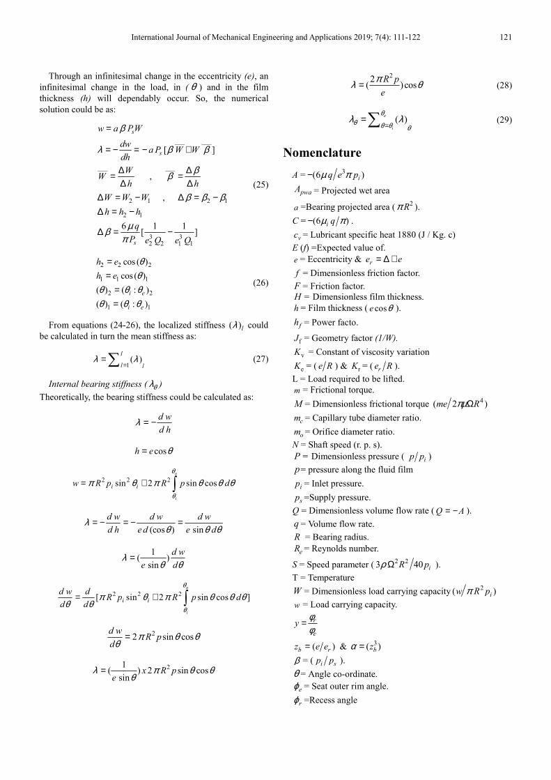
Through an infinitesimal change in the eccentricity (e), an

infinitesimal change in the load, in ( θ ) and in the film

thickness (h) will dependably occur. So, the numerical

solution could be as:

___ ___

___ ___

2 1 2 1

2 1

3 32 2 1 1

[ ]

,

,

6 1 1[ ]

s

s

s

w a PW

dwa P W W

dh

WW

h h

W W W

h h h

q

P e Q e Q

β

λ β β

ββ

β β β

µβπ

=

= − = − +

∆ ∆= =∆ ∆

∆ = − ∆ = −∆ = −

∆ = −

(25)

2 2 2

1 1 1

2 2

1 1

cos ( )

cos ( )

( ) ( : )

( ) ( : )

i e

i e

h e

h e

θθ

θ θ θθ θ θ

==

==

(26)

From equations (24-26), the localized stiffness ( )lλ could

be calculated in turn the mean stiffness as:

1( )

l

l lλ λ

==∑ (27)

Internal bearing stiffness ( θλ )

Theoretically, the bearing stiffness could be calculated as:

d w

d hλ = −

cosh e θ=

2 2 2sin 2 sin cos

o

i

i iw R p R p d

θ

θ

π θ π θ θ θ= + ∫

(cos ) sin

d w d w d w

d h e d e dλ

θ θ θ= − = − =

1( )

sin

d w

e dλ

θ θ=

2 2 2[ sin 2 sin cos ]

o

i

i i

d w dR p R p d

d d

θ

θ

π θ π θ θ θθ θ

= + ∫

22 sin cos

d wR p

dπ θ θ

θ=

21( ) 2 sin cos

sinx R p

eλ π θ θ

θ=

22( )cos

R p

e

πλ θ= (28)

( )e

i

θθ θ θ θ

λ λ=

=∑ (29)

Nomenclature

A =3(6 )iq e pµ π−

pwaA = Projected wet area

a =Bearing projected area (2Rπ ).

C = (6 )i qµ π− .

vc = Lubricant specific heat 1880 (J / Kg. c)

E (f) =Expected value of.

e = Eccentricity & re e= ∆ +

f = Dimensionless friction factor.

F = Friction factor.

H = Dimensionless film thickness.

h = Film thickness ( cose θ ).

fh = Power facto.

fJ = Geometry factor (1/W).

vK = Constant of viscosity variation

eK = ( e R ) & rK = ( re R ).

L = Load required to be lifted.

m = Frictional torque.

M = Dimensionless frictional torque 4( 2 )me RπµΩ

cm = Capillary tube diameter ratio.

om = Orifice diameter ratio.

N = Shaft speed (r. p. s).

P = Dimensionless pressure ( ip p )

p= pressure along the fluid film

ip = Inlet pressure.

sp =Supply pressure.

Q = Dimensionless volume flow rate ( Q A= − ).

q = Volume flow rate.

R = Bearing radius.

eR = Reynolds number.

S = Speed parameter (2 23 40 iR pρ Ω ).

T = Temperature

W = Dimensionless load carrying capacity2( )iw R pπ

w = Load carrying capacity.

r

e

yφφ

=

( )b rz e e= & 3( )bzα =

β = ( i sp p ).

θ = Angle co-ordinate.

eϕ = Seat outer rim angle.

rϕ =Recess angle


iθ =Inlet flow angle.

eθ = Outlet flow angle.

∆= Recess depth

T∆ = Temperature rise

ρ = Lubricant density.

σ = Dimensionless surface roughness parameter. 2oσ = Variance of the film thickness.

λ = Bearing stiffness.

aλ = Axial stiffness

tλ = Transversal stiffness

rλ = Radial stiffness

θλ = Internal stiffness

µ =Lubricant viscosity.

Ω =Rotational speed

Suffix

c capillary

o orifice

e exit

i inlet

th theoretical

n numerical

References

[1] Ahmad W. Yacout, Ashraf S. Ismaeel, Sadek Z. assab, "The combined effects of the centripetal inertia and the surface roughness on the hydrostatic thrust spherical bearing performance", Tribolgy International Journal 2007, Vol. 40, No. 3, 522-532.

[2] Ahmad W. Y. Elescandarany, “The Effect of the fluid film variable viscosity on the hydrostatic thrust spherical bearing performance in the presence of centripetal inertia and surface roughness (Part 1 Un-recessed fitted bearing)”, The International Journal of Mechanical Engineering and Applications 2018, Vol. 6, No. 1, pp. 1-12.

[3] Ahmad W. Y. Elescandarany, “The Effect of the fluid film variable viscosity on the hydrostatic thrust spherical bearing performance in the presence of centripetal inertia and surface roughness (Part2 Recessed fitted bearing)”, The International Journal of Mechanical Engineering and Applications 2018, Vol. 6, No. 3, pp. 73-90.

[4] Ahmad Waguih Yacout Elescandarany, “Design of the

Hydrostatic Thrust Spherical Bearing with Restrictors (Fitted Type)“, The International Journal of Mechanical Engineering and Applications 2019 Vol. 7, No. 2, pp. 34-45.

[5] Kane N. R., Sihler J. and Slocum A. H. "A hydrostatic rotary bearing with angled surface self-compensation", Precision Engineering 2003, 5321, pp: 1–15.

[6] Xiaobo Z., Shengyi L., Ziqiang Y. and Jianmin W. "Design and Parameter Study of a Self-Compensating Hydrostatic Rotary Bearing" International Journal of Rotating Machinery, Volume 2013, Article ID 638193, pp: 1-10.

[7] Yuan K., De-Xing P., Yu-Hong H. and Sheng-Yan H." Design for static stiffness of hydrostatic bearings: double-action variable compensation of membrane-type restrictors and self-compensation". Industrial Lubrication and Tribology 2014, Vol. 66, · No. 2, pp: 322–3343.

[8] Xu C. and Jiang S., "Analysis of the static characteristics of a self-compensation hydrostatic spherical hinge". J. Tribolohy T. ASME 2015; Vol. 137, No. 4: 044503-044503-5.

[9] Khaksea P. G., Phalleb V. M. and Manthac S. S. "Comparative Performance of a Non-recessed Holeentry Hybrid/Hydrostatic Conical Journal Bearing Compensated with Capillary and Orifice Restrictors", Journal of Tribology in Industry 2016, Vol. 38, No. 2, pp: 133-148.

[10] Zhifeng Li., Yumo W., Ligang C., Yongsheng Z., Qiang C. and Xiangmin D., "A review of hydrostatic bearing system: Researches and Applications", Advances in Mechanical Engineering 2017, Vol. 9, No. 10, pp: 1–28.

[11] Alexander Slocum, "Externally Pressurized Fluid Film Bearings", Precision Machine Design, ME EN 7960 – Non-Contact Bearings – Topic 11, pp: 1-47.

[12] Alexander Slocum, Paul Scagnetti, Nathan Kane and Christoph Brunner," Design of self-compensated, water-hydrostatic bearings" Journal of Precision Engineering 1995, Vol. 17, No. 3, pp: 173-185.

[13] Zhao Yang Dong, Sheng-Yen Hu, Chao-Ping Huang and Yuan Kang" Static Characteristic of Self-compensated Hydrostatic Bearing" Proceedings of the International Conference on Environmental Science and Sustainable Energy, 2017.

[14] Mohit Agarwal, "Non-Dimensional Parameters of a Membrane-Type Restrictor in an Opposed Pad Hydrostatic Bearing for High Static Stiffness", International Journal of Science and Research 2018, Vol. 7 No. 7, pp: 1306-1313.

[15] Antony Raymond Wong," Design of low cost hydrostatic bearing", Master thesis, Massachusetts Institute of Technology, 2019.

design of self-restriction hydrostatic thrust spherical

Documents