Design of Wood Highway Sound Barriers Thomas E. Boothby Courtney B. Burroughs Craig A. Bernecker Harvey B. Manbeck Michael A. Ritter Stefan Grgurevich Stephen Cegelka Paula D. Hillbrich Lee

United States Department of Agriculture Forest Service Forest Products Laboratory National Wood in Transportation Information Center Research Paper FPL−RP−596

In cooperation with the United States Department of Transportation Federal Highway Administration

Abstract As new and existing U.S. residential areas and high volume highways continue to intermingle, traffic noise abatement procedures continue to be important. This study investigated the acoustic effectiveness, public acceptance, and structural requirements of various designs and types of sound barriers. In addition, the acoustic effectiveness of a prototype sound barrier is reported. Results are presented on the acoustic effectiveness from in situ measurements of one cement-bonded composite panel barrier and four precast concrete, two plywood, two glued-laminated, and three post and panel barriers. The research on public acceptance of sound barriers focused on the perception of visual compatibility. Based on results from semantic-differential and individual ratings, wood and concrete barrier designs were perceived to have favored “rural” qualities. Data collected during the research on acoustic effectiveness and public acceptance were used to develop structural requirements and construction details for a prototype wood sound barrier. The prototype wood sound barrier provided insertion losses of 15 dB or greater, exceed-ing the 10-dB acceptable performance for a highway sound barrier.

Keywords: Wood barrier, sound barrier, barrier effective-ness, acoustics

Acknowledgment This study was made possible by cooperative agreement FP–94–2274.

June 2001 Boothby, Thomas E.; Burroughs, Courtney B.; Bernecker, Craig A.; Manbeck, Harvey B.; Ritter, Michael A.; Grgurevich, Stefan; Cegelka, Stephen; Lee, Paula D. Hillbrich. 2001. Design of wood highway sound barriers. Res. Pap. FPL-RP-596. Madison, WI: U.S. Department of Agriculture, Forest Service, Forest Products Laboratory. 69 p.

A limited number of free copies of this publication are available to the public from the Forest Products Laboratory, One Gifford Pinchot Drive, Madison, WI 53705–2398. Laboratory publications are sent to hundreds of libraries in the United States and elsewhere.

The Forest Products Laboratory is maintained in cooperation with the University of Wisconsin.

The use of trade or firm names is for information only and does not imply endorsement by the U.S. Department of Agriculture of any product or service.

The United States Department of Agriculture (USDA) prohibits discrimina-tion in all its programs and activities on the basis of race, color, national origin, sex, religion, age, disability, political beliefs, sexual orientation, or marital or familial status. (Not all prohibited bases apply to all programs.) Persons with disabilities who require alternative means for communication of program information (Braille, large print, audiotape, etc.) should contact the USDA’s TARGET Center at (202) 720–2600 (voice and TDD). To file a complaint of discrimination, write USDA, Director, Office of Civil Rights, Room 326-W, Whitten Building, 1400 Independence Avenue, SW, Wash-ington, DC 20250–9410, or call (202) 720–5964 (voice and TDD). USDA is an equal opportunity provider and employer.

Units of Measurement Measurements included in the text, tables, and some figures are expressed in SI units. In other figures, notably those of design details used to develop the test sound barrier, meas-urements are expressed in inch–pound units. The conversion factors for these units are shown in the following table.

Inch–pound unit Conversion

factor SI unit

inch (in.) 25.4 millimeter (mm) foot (ft) 0.3048 meter (m) pound force/square inch (lb/in2) 6.894 kilopascal (kPa) pound force/square foot (lb/ft2) 47.88 pascal (Pa)

Contents Page Introduction .......................................................................... 1

Project Overview .............................................................. 1 Literature Review ............................................................. 2

Acoustic Effectiveness.......................................................... 3 Barrier Selection ............................................................... 3 In Situ Testing .................................................................. 4 Determination of Normalized Insertion Loss ................... 4 Determination of Transmission Loss................................ 9 Analysis of Normalized Insertion Loss and Transmission Loss ............................................................ 9

Public Acceptance .............................................................. 15 Selection of Design Types .............................................. 15 Slides .............................................................................. 15 Testing ............................................................................ 17 Analysis of Rating Scales ............................................... 20

Structural Requirements for Prototype Barrier ................... 35 Systematic Approach to Design...................................... 35 Design of Test Sound Barrier ......................................... 38

Acoustic Effectiveness of Test Sound Barrier .................... 44 Test Procedures............................................................... 45 Site Plan.......................................................................... 46 Testing Sequence............................................................ 46 Determination of Insertion Loss ..................................... 48 Discussion of Results...................................................... 48

Conclusions ........................................................................ 49 Acoustic Effectiveness of Existing Barriers ................... 49 Public Acceptance .......................................................... 49 Systematic Design Details .............................................. 49 Acoustic Effectiveness of Test Barrier ........................... 49 Recommendations........................................................... 49

Literature Cited................................................................... 50 Appendix A—Existing Barriers Used in Acoustic In Situ Testing .................................................................... 52 Appendix B—Computer Edited Images Used in Public Acceptance Evaluations...................................................... 54 Appendix C—Structural Design Example.......................... 59 Appendix D—Highway Sound Barrier Plans..................... 63

Design of Wood Highway Sound Barriers Thomas E. Boothby, Associate Professor Courtney B. Burroughs, Senior Research Associate Craig A. Bernecker, Associate Professor Harvey B. Manbeck, Distinguished Professor The Pennsylvania State University, University Park, Pennsylvania

Michael A. Ritter, Assistant Director Forest Products Laboratory, Madison, Wisconsin

Stefan Grgurevich , former Graduate Student Stephen Cegelka, former Graduate Student The Pennsylvania State University, University Park, Pennsylvania

Paula Hillbrich Lee, former General Engineer Forest Products Laboratory, Madison, Wisconsin

Introduction Project Overview As new and existing U.S. residential areas and high volume highways continue to intermingle, traffic noise abatement procedures will always be of importance. Since the mid-1960s, traffic noise analysis and control procedures, primarily by State and Federal governments, have increased. Agencies such as individual State Departments of Transpor-tation, the Federal Highway Administration (FHWA), the U.S. Environmental Protection Agency (EPA), and the Transportation Research Board (TRB) have provided fund-ing and research of traffic noise control.

The three primary ways to control traffic noise are by source, receiver, and path (FHWA 1994c). Source control imposes regulations on emissions of trucks, motorcycles, and buses. Receiver control includes carefully planned zoning, building codes, land ownership control, and site planning. Path control attempts blocking or lengthening the path trav-eled by traffic noise. Path control consists of either shifting the vertical alignment of the road surface, which may shield traffic noise, or using a sound barrier, which attempts to reduce sound levels on the residential side of the barrier by altering the direct path that traffic noise follows from the highway (source) to the resident (receiver). Government agencies concentrate much of their research on the imple-mentation of sound barriers (FHWA1994c).

Highway sound barriers placed near residential neighbor-hoods provide an effective tool to control traffic noise. Bar-riers can be constructed of earth, precast concrete panels, concrete block, brick, wood, metal, or a combination of

these (FHWA 1994a). In 1992, total length of highway sound barriers in the United States exceeded 1,486 km (FHWA 1994b). Cohn and Harris (1990) reported that wood and the combination of wood and earth berm account for approximately 17% of all sound barriers on U.S. highways.

From 1991 to 1996, annual expenditures for sound barriers in most States exceeded $2 million per year (FHWA 1994c). This spending included type 1 and type 2 projects. Type 1 projects involve the simultaneous construction of the high-way and sound barrier; type 2 projects involve construction of the sound barrier after the highway has been built and traffic noise has become a problem. Most States design barriers to attain an insertion loss of 5 to 10 dB; any barrier providing less than this may be considered cost inefficient. The FHWA (1994c) reported that a barrier attaining this acoustic effectiveness level would cost approximately $12/ft2, regardless of material. Cost per residence is another way to measure cost effectiveness. Costs ranging from $8,000 per residence in Washington to $40,000 in Maryland have been reported (FHWA 1994c). Cost can also be meas-ured by dollars per residence per A-weighted sound level (dBA) loss. Costs reported in this manner are preferred because dBA values provide a better indication of the effectiveness of the barrier. The average initial costs of a wood barrier are much less than those of a concrete barrier. However, the effects of weathering cause maintenance costs for wood barriers to exceed those of concrete barriers. The annual cost for both wood and concrete barriers compared with their respective design lives are very competitive (FHWA 1994c). A computer program is available for designing cost-effective barriers (Anderson and others 1997).

2

Literature Review Acoustic Effectiveness The acoustic effectiveness of sound barriers can be measured in terms of insertion loss and transmission loss. Insertion loss is the noise reduction that a barrier causes if it is built between the source and receiver. Transmission loss is a measure of how much sound travels through a barrier. To-gether, these two measures give the designer a sense of the acoustic effectiveness of a proposed barrier.

Insertion loss is a measurement that includes the diffraction of sound waves over the top of a sound barrier. Because most barriers block sound transmission, most sound that reaches receivers behind the barrier diffracts over the top of the barrier. The importance of sound waves diffracting over the top of the barriers is reinforced by research on the special treatment of barrier tops. Absorption and a T-profile on top of a barrier increase barrier insertion loss 1 to 1.5 dB (May and Osman 1980). Absorptive cylinder tops increase inser-tion loss 2 to 3 dB (Fujiwara and Furuta 1991), and a phase-delay device produces increases of 3 to 5 dB (Amram and others 1987). Another variable that influences insertion loss is the height of a barrier. Increasing the height, however, has a limit when the increased benefit is no longer cost effective. The height limitations reported by researchers vary from 4.0 m (May and Osman 1980) to 4.9 m (Lambert 1978). If a parallel barrier in installed on the opposite side of the high-way, the insertion loss is further reduced by approximately 2 dB, because sound waves are reflected by one barrier towards and over the opposite barrier (Bowlby and others 1987). Although absorptive material does not significantly affect the insertion loss of a single barrier (May and Osman 1980), surface absorption reduces reflection from the barri-ers and improves the insertion loss of parallel barriers by 3.5 to 4.5 dB (Bowlby and others 1987).

In contrast, transmission loss and its influence on insertion loss is a concern to many designers of highway sound barri-ers. Because the mass density of wood is lower than that of concrete or steel, designers are concerned that when wood barriers are not sufficiently thick, the low transmission loss will counteract the insertion loss. In other words, sound waves will travel through the barrier and reduce the shield-ing effect of the barrier between the receiver and sound source. However, according to Kurze and Anderson (1971), transmission through barriers can be ignored if the surface mass of the barrier is greater than 20 kg/m2. This assumes that there are no resonance or coincidence effects to reduce transmission losses. If such effects existed, damping would be necessary for the barrier. Resonance and coincidence effects do exist in steel sound barriers. Behar and May (1980) reported that the damping of steel barriers resulted in a 4-dB increase in insertion loss.

Public Acceptance The need for highway sound barriers comes from the desire of a community to reduce public annoyance caused by traffic noise. Therefore, public acceptance is a critical evaluation criterion for sound barrier designs. According to Cohn and Bowlby (1984), community acceptance has two components: the perception of noise mitigation and the perception of visual compatibility. Even though both components are subjective, it is necessary to address them for a barrier to satisfy the desires of the community.

Quantification of the perception of noise mitigation has been attempted by several methods. One method widely used by professionals is equating an average sound level with a percentage of the population that would be annoyed by the highway noise (Schultz 1982). By correlating average day and night sound levels with the percentage of population describing themselves as “highly annoyed” by transportation noise, designers only need to reduce noise levels that cause annoyance in a specified percentage of the population. How-ever, because it is unrealistic to expect an insertion loss of much more than 15 dB from a sound barrier (May and Osman 1980) and additional insertion loss might be needed to satisfy this sound criterion, other strategies might have to be used to gain public acceptance. Consequently, the perception of visual compatibility must be considered.

The public perception of visual compatibility is considered to be more important than the acoustic performance in stud-ies of perceived effectiveness (Cohn 1981). Many people perceive landscaping to reduce noise levels, even though the measured loss due to landscaping is negligible. Although it is impossible to objectively quantify public perception con-cerning the aesthetics of a highway sound barrier, character-istics of barriers have been identified that influence a com-munity’s acceptance of a barrier.

Cohn and Bowlby (1984) identified these characteristics to be size and mass, material selection and color, landscaping, and public involvement. The public does not favor the use of tall or massive sound barriers. The public also believes that materials should be perceived as compatible with the sur-rounding environment. Consequently, earthen berms are usually the most easily accepted material for a barrier and metallic structures the most poorly received. Next, the public usually considers landscaping to soften the visual impact of sound barriers. Landscaping on both sides of the barrier can naturally camouflage the barrier so that it blends into the natural surroundings. Finally, public involvement in the design of the barriers increases the level of acceptance. Involvement in the design makes the barrier more visually compatible to the community. Taking all identified charac-teristics into account in the evaluation of barrier design will help the community view the barrier as both effective and less intrusive.

3

Structural Requirements and Durability Sound barrier designs follow the Guide Specifications for Structural Design of Sound Barriers (AASHTO 1989a), the 1994 Uniform Building Code (UBC 1994) or the BOCA National Building Code (BOCA 1987), regulations from individual State Departments of Transportation, and design manuals related to material type such as the ACI 318–95 (ACI 1995) and the National Design Specification for Wood Construction (AF&PA 1991).

Wood sound barriers are typically designed with a panel section attached to posts. The panels can be made of timber planks or glued-laminated panels. The posts are normally large solid-sawn timbers or glued-laminated timbers, but they may be steel or concrete. The primary live loads are wind loads. In most cases, no vertical loads are applied, and the self-weight of the sound barrier and its foundation are used in determining the soil-bearing capacity. Other loads may include earth loads, for which the barrier functions as a retaining wall, and traffic or impact loads. Traffic impact loads are not necessary to apply unless the sound barrier is combined with a traffic barrier (AASHTO 1989b). In addi-tion, sound barriers on structures, such as bridges and retaining walls, as well as traffic barriers require certain specifications beyond those for ground-mounted barriers.

Durability is a measure of the length of time a sound barrier remains aesthetically acceptable and structurally and acous-tically effective. Weathering and decay are the main con-cerns for a wood sound barrier. Weathering, which causes dimensional changes in wood, results in cracking, checking, and warping, which causes gaps to develop in the barrier, decreasing transmission loss, structural integrity, and aes-thetics. Decay results in wood decomposition, which affects the structural and acoustic performance of the barrier.

Preservative treatments and water repellents are commonly used to resist decay and dimensional changes, respectively, in exterior wood applications. Oilborne preservatives pro-vide resistance to weathering and decay; waterborne pre-servatives provide only decay resistance (FPL 1999). Pre-servatives are widely used on wood transportation structures such as bridges, guardrails, and retaining walls. Oilborne preservatives used in timber bridge applications are creosote, pentachlorophenol, and copper naphthenate. These preserva-tives cause skin irritations and should not be used in applica-tions that involve human contact (FPL 1999). Some pre-servatives may also darken the surface of the barrier somewhat, lead to bleeding when the barrier is in direct sunlight, and produce a slightly oily surface that makes additional surface preparation difficult. Waterborne pre-servatives primarily used in softwood bridge applications include chromated copper arsenate (CCA), ammoniacal copper arsenate (ACA), and copper zinc arsenate (ACZA). Waterborne preservatives will accommodate the variety of wood species that are typically used in wood sound barriers.

These preservatives leave the surface clean and can be used where human contact is expected. With the use of preserva-tive treatment and water repellent, wood sound barriers have an expected service life of 15 to 25 years (FHWA 1994c). Although the chemicals used for treating wood are regulated under EPA pesticide regulations, the treated wood is not subject to additional regulation, that is, not considered a pesticide (Webb and Gjovik 1988). The research results on leaching rates of preservatives from treated wood are few and inconclusive, but research to date indicates that leached copper, chromium, and arsenic have little mobility in soil (Lebow 1996).

Acoustic Effectiveness The acoustic effectiveness of concrete and wood sound barriers was determined by in situ testing of existing sound barriers. The in situ testing of different design types and materials was necessary because of the lack of extensive data on insertion and transmission losses of various barrier types. The goal of this testing was to determine the insertion and transmission losses of various wood and concrete barriers. Data were normalized to allow for direct comparison be-tween different barrier design types. The objective was to determine if wood and concrete barriers are equivalent in terms of acoustic effectiveness.

Barrier Selection The wood barrier designs investigated in the in situ testing are listed in the Guide Specification for Highway Noise Barriers (NFPA 1985). The following three design types of barriers are listed:

1. Timber plank (also called post and panel) barriers, made of heavy timber posts and dimension lumber panels

2. Plywood barriers, made of plywood panels, usually sup-ported by dimension lumber

3. Glued-laminated barriers, made of glued-laminated wood members

The barriers selected for testing were located on flat land and were easily accessible from both sides. Eight wood barriers were selected for in situ testing: three glued-laminated, three post and panel, and two plywood. The glued-laminated barriers were located outside Washington, DC, on I-495; near Troy, New York, on Route 7; and in Erie, Pennsyl-vania, on I-79. Two post and panel barriers were located on the Hutchinson River Parkway outside New York and one on the Long Island Expressway. In situ tests were also per-formed on a cement-bonded composite post and panel bar-rier in Madison, Wisconsin. This barrier was made of ce-ment-bonded composite wood fiber panels and precast concrete posts. The two plywood barriers were located at a truck weigh station across the Pennsylvania/Maryland border on I-83 and outside Baltimore on I-95. In addition to the

4

wood barriers and composite barrier, four precast concrete panel barriers were identified for in situ testing. The concrete barriers were located on I-695 outside Baltimore, on I-95 outside New York City, on Route 24 outside Whippany, New Jersey, and on I-78 in New Jersey. Photographs of the barriers are in Appendix A.

In Situ Testing Insertion losses of the selected barriers were determined using the indirect predicted method of the American Na-tional Standard—Methods for Determination of Insertion Loss of Outdoor Noise Barriers (ANSI 1987). Even though this standard does not prescribe the use of a particular pre-diction method, it does specify the following:

1. The type of ground and topography between the source and receiver should be included in the predictions.

2. The prediction model should be validated over the relevant range of source/receiver distances and for the relevant to-pography and type of ground.

3. If wind velocity and temperature gradients are not consid-ered in the prediction method, then the indirect predicted method should only be used for calm wind conditions, which are defined as 1.2 m/s (2.7 m/h).

The prediction model used is outlined in the FHWA High-way Traffic Noise Prediction Model (FHWA 1978b). This method was used to determine insertion losses at distances of 3.1, 7.6, and 15.3 m behind the barriers used for the in situ measurements. A measured free-field sound level was ad-justed to predict sound levels that would occur at the re-ceiver positions in the absence of the barrier. Only four microphones were available for in situ testing; therefore, two different microphone setups were used to obtain sufficient measurements to determine transmission and insertion losses at 3.1, 7.6, and 15.3 m. The two microphone setups were used for two separate recordings or cuts (Figs. 1 and 2). Figure 1 illustrates the locations of the microphones for cut 1. Microphone 1 was located next to the road, allowing for sound level to be corrected for differences in traffic noise levels between the two cuts. Microphones 3 and 4 helped determine the transmission losses of different barriers. Mi-crophone 3 recorded the free-field sound levels used to predict sound levels in front of the barrier and at 3.1, 7.6, and 15.3 m from the barrier in the absence of the barrier. Figure 2 illustrates the locations of the microphones for cut 2. Microphone 1 was located next to the road as in cut 1 to allow for sound level adjustment between cuts. Microphones 2, 3, and 4 were located 3.1, 7.6, and 15.3 m, respectively, behind the barrier to help determine insertion losses of the barriers.

Using these two setups with a multi-channel tape recorder, sound levels were measured simultaneously at each set of four locations. Simultaneous recordings eliminated the need

to adjust all sound levels for changes in traffic noise levels. The only adjustments required were between cuts because the free-field sound level was measured in cut 1 by micro-phone 3 and the sound levels behind the barrier were meas-ured in cut 2. Thus, two adjustments were necessary to determine insertion loss: (1) the free-field sound level meas-ured in cut 1 by microphone 3 was adjusted to predict the pre-barrier sound level at the receiver position, and (2) the sound levels measured in different cuts were adjusted for changes in the traffic noise levels that occurred between cuts. Both adjustments were made after the recordings were reduced to determine the sound levels. In contrast, transmis-sion loss did not require a sound level correction between cuts because all the recordings necessary to determine transmission loss were taken in cut 1.

For the measurements made on the side of the barrier oppo-site the traffic, amplification was required prior to recording to increase levels of the recorded signal above the electronic background noise levels, although when amplification was used, the effect of electronic noise was reduced. Amplifiers had no effect on nontraffic background noise present at the measurement sites.

Determination of Normalized Insertion Loss Analysis of Recordings Readings on a standard sound level meter using the A-scale incorporate a frequency-weighting network approximating

Figure 1—Microphone locations for cut 1.

Figure 2—Microphone locations for cut 2.

5

the variation of ear sensitivity with frequency to tones of a 40-dB sound pressure level. The multi-channel recordings of the two cuts were analyzed to determine average sound pressure levels in the third-octave bands from 200 Hz to 5 kHz. Below 200 Hz, A-weightings are greater than 10 dB, and above 5 kHz, the level of traffic noise decreases. Thus, it is in the 200-Hz to 5-kHz range where the contribution of traffic noise to A-weighted noise levels is dominant and therefore of primary concern for reduction by a sound bar-rier. Because traffic varied during recordings, different averages were taken from continuous recordings for ap-proximately 15 min. At sites where traffic was heavy and the source noise levels were high and constant, averages were taken when the traffic was heavy and continuous. Correc-tions for background noise were unnecessary. At sites where traffic was not heavy or continuous, averages during quiet and noisy periods were taken. These two averages were then used to remove the effect of background noise. Even with the correction for background noise, insertion loss predic-tions were based on data taken when traffic noise levels were at a maximum, thereby reducing the effects of background noise on the measured levels.

Reduction of the recorded signals was performed by a multi-channel analyzer. Corrections were applied for differences in sensitivity of each measurement channel. The determination of absolute sound pressure levels was not required because results reported here are differences in sound pressure levels; absolute levels are not presented. Output from the analyzer resulted from the following:

( )volt1/log20 msv VL = (1)

where Lv is recorded sound level referenced to 1 volt, and Vrms is the root mean square of the measured voltage.

The units of this formula are decibels referenced to 1 volt (dB re 1volt). All recordings were less than 1 volt; therefore, the resulting levels are negative. Repeat measurements were used to establish means and variations for purposes of esti-mating random measurement errors and identifying invalid data points.

The corrections for differences in traffic noise levels be-tween the two cuts were made because the measurement of the free-field sound levels was made in cut 1 and the meas-urements of sound levels behind the barrier were made in cut 2. These corrections involved taking the difference be-tween measurements taken in the two cuts of microphone 1, which remained in the same location. These corrections were added to the sound levels for microphone 3 during cut 1 so that these levels, after correction for differences in distance, could be compared directly with levels measured during cut 2.

Pre-barrier sound levels occurring at reference positions behind the barrier were predicted using the corrected sound

levels for microphone 3 in cut 1. This required two steps: (1) predicting the spreading loss and accounting for ground effects that occurred between microphone 3 and the refer-ence location and (2) correcting for the sensitivity differ-ences between the microphones.

Sound Level Predictions The prediction model used to account for the spreading loss and ground effects occurring between the reference free-field location (microphone 3 in cut 1) and the reference locations behind the barrier is described in the FHWA Highway Traffic Noise Prediction Model (FHWA 1978b). This model calculated the spreading loss and ground effects as

( ) α+=∆ 10s /log10 DDL (2)

where

∆Ls is change in sound level between recorded free-field sound level and receiver location,

D perpendicular distance between roadway and receiver location on nontraffic side of barrier,

D0 distance between roadway and location of micro-phone 3 in cut 1 where free-field sound level was measured, and

α site parameter whose value depends upon site condi-tions, α = 0 for acoustically hard (paved) surfaces and α = 1/2 for absorptive (landscaped) surfaces.

Preliminary pre-barrier sound levels at sites on the nontraffic side of the barrier were predicted. When ground conditions, such as a soft surface in front of and a paved surface behind the barrier, changed between the source and receiver, this formula was used twice, once for the first ground condition, then for the second ground condition.

The prediction model satisfied the three requirements outlined in ANSI S12.8 (ANSI 1987). First, the model ac-counts for ground and topography between the source and receiver. Second, Highway Noise Measurements for Verifi-cation of Prediction Models (FHWA 1978b) provide exten-sive results concerning the field validation of the prediction model over the relevant range of source/receiver distances and for the relevant topography and type of ground. This reference provides statistical data showing that the noise prediction model presents theoretical values close to meas-ured values. Third, recorded wind velocity and temperature data during tests showed that wind velocities less than 7 km/s did not affect the results of the prediction model for the receiver distances used in this project. Because wind conditions during the in situ testing were calm (<7 km/s), wind velocity and temperature gradients should not have affected the predictions of insertion and transmission losses.

6

Because the four microphones used in the in situ testing had slightly different sensitivities, they were calibrated with the associated recording instrumentation. The in situ testing was conducted twice: in the fall of 1994 (calibration 1) and the spring of 1995 (calibration 2). Microphones and recording equipment were calibrated for both sets of tests. The calibra-tion was done by placing a pistophone, which produces a sound level of 124 dB at a frequency of 250 Hz, over each microphone to produce a sound recording. The recordings from each microphone were then reduced with the same equipment used to reduce all the measurement data to obtain the voltage levels that corresponded to the 124-dB calibra-tion sound pressure level. Calibration 1 was used for all the in situ testing except the two tests in New Jersey and the test on the plywood barrier outside Baltimore. Calibration 2 was used for these tests. The calibration results are given in Table 1. Because of problems in availability of microphones, different microphones were used for each calibration, which could account for the differences in the calibration values listed in Table 1.

The correction for the prediction of pre-barrier sound levels was simply the difference between the free-field reference microphone, which in all cases was microphone 3, and the receiver microphone, which was either microphone 2, 3, or 4. The preliminary prediction was corrected for differences in microphone sensitivity by taking this difference and add-ing it to the preliminary prediction.

Background Noise Adjustment The final correction necessary to estimate the insertion loss for barriers was to compensate for the effects of background noise. Background noise in a recording increases recorded sound levels, causing a decrease in the estimated insertion or transmission loss. The cause of background noise was either electronic noise produced by the recording equipment or by sources of nontraffic noise on the nontraffic side of the barrier. If traffic noise is constant and loud enough and an amplifier is used to increase the signal of the microphone recorded on the nontraffic side of the barrier, background noise has no effect on the recorded sound levels. However, when traffic noise is not loud enough, even an amplifier does not allow for compensation for background noise.

Compensation for the background noise from the recordings involved manipulating sound levels recorded during noisy and quiet periods. First, ratios of measured increase in sound pressure at roadside and on the nontraffic side of the barrier were found. The two ratios are expressed in terms of source pressures as follows:

2

Qs

ns

1

=

P

Px (3)

( ) ( )( ) ( )

1212n

2nn

2n

2Qn

2 >>+

+= xx

PP

PPx (4)

where

x1 is measured increase at roadside,

x2 measured increase behind barrier,

Psn source pressure under noisy conditions,

PsQ source pressure under quiet conditions,

Pnn nontraffic side pressure under noisy conditions,

PnQ nontraffic side pressure under quiet conditions, and

Pn background pressure.

By assuming that (Pnn/Pn

Q)2 = (Psn/Ps

Q)2 = x1, the ratio (Pn/Pn

Q)2 in terms of x1 and x2 is

(Pn / PnQ)2 = y = (x1 − x2) / (x2 − 1) (5)

Equation (5) requires that the sound levels acquired from the recordings be converted to sound pressures x1 and x2. By taking the difference between “noisy” and “quiet” periods, ∆i, the sound levels can be converted to a ratio of sound pressure with

10/10 iix ∆= (6)

The variable y for each pair of noisy and quiet recordings can be determined for every frequency. The difference be-tween quiet recordings of the microphone of interest and the background noise level is

A = −10 log(1 + 1/y) (7)

The background noise level is determined by logarithmically subtracting the value A from the sound level of the micro-phone of interest.

According to ANSI S12.8 (ANSI 1987), if the difference between the recorded noisy sound level and background noise is less than 4 dB, the sound level is reported as being masked by the background noise. All recorded noisy sound levels that were within 4 dB of the background noise were deleted from the data sets.

Table 1—Microphone calibration results

Calibrated sound pressure for test microphones 1 to 4 (dB re 1 V)

1 2 3 4

Calibration 1 3.6 1.7 5.2 3.1

Calibration 2 4.0 0.1 0.9 0.3

7

Estimated Insertion Loss Test results are absent or incomplete for some barriers. Results for the three barriers tested in Erie, Pennsylvania, were not used because traffic was light and amplifiers were not available; thus, the recorded levels were contaminated by electronic noise. In addition, background noise was a prob-lem for recordings for the precast concrete barrier on I-695 outside Baltimore and the post and panel barrier on the Hutchinson River Parkway. The insertion losses at the fre-quencies masked by background noise were deleted from the data set. Consequently, data were truncated for these barri-ers. Background noise also masked a few frequencies of recordings for the I-83 Maryland plywood barrier, the Route 7 New York glued-laminated barrier, and the Long Island Expressway post and panel barrier. Recordings from cut 2 for the post and panel barrier on the Long Island Expressway were lost.

The estimated insertion losses presented in Table 2 range from 10 to 20 dB. However, insertion loss did not increase with frequency as expected. Also, there appears to be no correlation between the height of the barrier and insertion loss. For example, the 2.5-m-high barrier on I-78 New Jersey had a greater insertion loss than did the 6.7-m-high barrier on I-95 Baltimore. The insertion losses were normalized to a common distance between the barrier and roadway and for a common height to remove the effect of these parameters. However, other parameters were not included in the nor-malization, such as the acoustic impedance of the ground and the topography around the barrier.

For most barriers, insertion loss decreased as the distance behind the barrier increased (Table 2). The exceptions were the barriers on I-78 New Jersey, on Route 24 New Jersey, on I-83 Maryland, on the Hutchinson River Parkway New York, and outside Madison, Wisconsin. The barriers on I-78 New Jersey, I-83 Maryland, and outside Madison were either situated on a berm or the ground rolled off behind the bar-rier. The barriers on the Hutchinson River Parkway were located far from the roadway (about 14 m). There were no unusual characteristics for the barrier on Route 24 New Jersey.

Normalization of Estimated Insertion Loss Variation was observed in the insertion losses within groups of barriers of similar design type. Much of the variation was due to differences in barrier height, topography, and distance of the barrier from the roadway. Barrier heights and dis-tances from the roadway are listed in Table 3 for each barrier.

In this study, the distance from the roadway to the barrier was assumed to be the distance from the edge of the road to the barrier, except for the I-95 Baltimore and I-495 Wash-ington DC barriers, where the traffic noise was assumed to be centered in the first lane and the distance was adjusted

accordingly. This adjustment was necessary because of the proximity of these barriers to the driving lanes.

The normalization of the insertion losses for the three differ-ent receiver locations involved the use of the prediction model presented in FHWA–RD–77–108 (FHWA 1978b). The normalization factor for a barrier was the difference between the predicted insertion loss and the predicted value at a given height and distance from the road on a flat site. The estimated insertion losses were normalized by subtract-ing the normalization factor from the estimated insertion loss. The insertion losses for all the barriers were normalized to a height of 4.3 m, a distance of 9.2 m from the roadway, and a flat site. The 4.3-m height was chosen because greater heights rarely produce a cost-effective benefit (May and Osman 1980, Lambert 1978). The 9.2-m distance was cho-sen because it was the mean of the source-to-barrier dis-tances for barriers used in this research project. Normaliza-tion of estimated insertion losses allowed direct comparisons of all test barrier types and locations.

The FHWA prediction model used for the normalization uses two equations. These equations vary slightly because the insertion loss of an earth berm is greater than that of a wall barrier. The equation for barrier insertion loss is

dB205 )2tanh(

)2( log 20IL

2/1

2/1≤+

ππ=

N

N (8)

where IL is predicted insertion loss, N = 2(rSB + rBR – dSB – dBR)/λ (distances defined in Fig. 3), and λ = (343/f).

The variable N is the Fresnel number, λ is acoustic wave-length in meters, and f is the frequency in hertz. Equation (8) was used for most of the barriers tested.

The earth berm equation used in the normalization is

dB238 )2tanh(

)2( log 20IL

2/1

1/2≤+

ππ=

N

N (9)

The only differences between Equations (8) and (9) are the constant added in Equation (9) and the maximum allowable value. Equation (9) was only used for the precast concrete barrier on I-78 New Jersey. This was the only barrier that was built on a berm, which is approximately 1.7 m high. Equation (8) was used for the remainder of the barriers.

Normalized Insertion Loss Data on normalized insertion losses are presented in Table 4. Incomplete data were the consequence of recordings masked by background noise. The same frequencies were masked for both the normalized and the estimated insertion losses, because normalized data were an adjusted version of estimated data.

Table 2—Estimated insertion loss at various distances behind the barrier a

Insertion loss (dB) for various barrier typesb

Precast concrete

Plywood

Post and Panel

Cement-bonded composite

I-695 Baltimore (6.7 m)

Distance behind

barrier (m)

I-95 NY (4.9 m)

Distance behind

barrier (m)

I-78 NJ (2.5 m)

Distance behind

barrier (m)

Rt.24 NJ (5.3 m)

Distance behind

barrier (m)

I-95 Baltimore (3.3 m)

Distance behind

barrier (m)

I-83 MD (4.3 m)

Distance behind

barrier (m)

Long Island Expressway, NY

(6.7 m) Distance behind

barrier (m)

Hutchinson River Parkway, NY 1

(1.9 m) Distance behind

barrier (m)

Hutchinson River Parkway, NY 2

(3.3 m) Distance behind

barrier (m)

Madison, WI (3.1m)

Distance behind

barrier (m)

Octave band

center fre-

quency (Hz) 3.1 7.6 15.3 3.1 7.6 15.3 3.1 7.6 15.3 3.1 7.6 15.3 3.1 7.6 15.3 3.1 7.6 15.3 3.1 7.6 15.3 3.1 7.6 15.3 3.1 7.6 15.3 3.1 7.6 15.3

200 12 10 9 13 —a 15 15 13 10 16 13 9 12 8 7 8 10 7 10 —a —a —a —a —a 7 2 10 2 0 4

250 12 11 8 11 —a 12 16 15 10 16 12 10 15 10 9 8 8 7 19 6 9 —a —a —a 8 10 9 5 4 3

315 11 10 7 15 —a 13 19 20 16 18 13 13 15 8 7 8 8 8 19 15 10 —a —a —a 11 11 12 12 8 17

400 12 11 9 16 —a 12 18 20 17 18 13 13 15 9 6 8 8 9 17 11 9 —a —a —a 10 12 11 8 8 12

500 13 12 10 18 19 13 16 18 16 19 15 17 16 9 5 8 8 10 13 12 9 —a —a —a 12 13 9 11 9 14

630 13 12 10 19 20 16 18 17 17 20 15 17 15 8 5 8 9 9 17 14 10 —a 8 6 11 12 9 12 11 16

800 13 12 11 18 20 15 18 18 17 20 16 18 14 7 5 9 10 9 18 13 11 —a 8 6 10 12 10 8 8 16

1,000 13 12 11 20 —a —a 18 18 18 20 16 18 14 7 5 8 8 8 19 14 12 —a 8 6 9 10 8 12 12 17

1,250 12 11 10 —a —a —a 19 18 17 20 16 17 15 8 6 7 8 8 20 13 11 — 8 5 8 10 7 12 14 17

1,600 11 11 9 —a —a —a 19 19 18 19 15 17 16 8 6 7 7 8 18 10 9 17 8 5 8 10 7 11 15 16

2,000 11 10 9 —a —a —a 19 18 17 18 14 15 16 10 7 8 9 9 19 13 10 14 7 5 8 9 6 10 15 14

2,500 10 9 8 —a —a —a 19 18 18 18 14 15 15 9 6 5 6 7 18 13 10 13 6 —a 8 9 7 9 15 16

3,150 9 8 7 —a —a —a 18 18 18 16 13 14 15 9 6 4 5 6 19 13 11 12 —a —a 9 10 7 8 16 18

4,000 10 8 8 —a —a —a 18 17 18 17 12 14 16 10 7 3 4 4 18 12 9 —a —a —a 10 11 8 10 16 16

5,000 —a 8 7 —a —a —a 18 17 19 18 12 17 17 11 9 3 —a 6 19 —a 11 —a —a —a 11 —a 10 7 14 17

aMissing values indicate that data were masked by background noise and removed from data set. bValues in parentheses indicate barrier height.

9

Comparison of the normalized results in Table 4 with the unaltered results in Table 2 indicates that normalization did not reduce the spread in data. However, some factors that could have contributed to data variability were not included in normalization, such as topography and ground impedance on each side of the barrier. Note that in spite of the spread in the insertion losses, there appears to be no correlation of the losses with the materials used for the barriers.

Determination of Transmission Loss The method used to determine transmission loss was similar to the method used to determine insertion loss. At first, transmission loss was determined by the recordings in the first cut, for which microphone locations are shown in Figure 1. Transmission loss was the difference in the sound levels between microphones 2 and 4. However, any sound reflecting off the barrier increased the sound level recorded by microphone 2. This pressure doubling artificially inflated

the sound level recorded by microphone 2 and, conse-quently, increased the estimated transmission loss for the barrier. To compensate for this pressure doubling, the sound level in front of the barrier (pre-barrier sound level) was predicted the same way as predicted for the insertion loss calculations. The pre-barrier sound level was predicted by taking the free-field sound level occurring at microphone 3 and adjusting for spreading loss and ground effects, as well as sensitivity differences between microphones. Having adjusted the predicted pre-barrier sound level and the sound levels measured by microphone 4 for background noise, the transmission loss was found to be the difference between the two adjusted sound levels. Because transmission loss was not affected by barrier height, barrier distance from the road, or topography, normalization was not necessary for the direct comparison of transmission loss values.

Transmission losses are presented in Table 5. Transmission losses could not be computed for the Madison barrier be-cause of the failure of microphone 4. All transmission losses in Table 5 are greater than 10 dB; most range from 15 to 25 dB. These values are greater than the values for the inser-tion losses, indicating that insertion losses are controlled primarily by diffraction over the top of the barriers. The transmission losses for the plywood and post and panel barriers were lower than those for the two glued-laminated barriers. These results do not take into account the transmis-sion loss data for the Madison barrier.

Analysis of Normalized Insertion Loss and Transmission Loss

Comparison of Normalized Insertion Loss With Estimated Transmission Loss To assist in the explanation of why the insertion loss did not increase with frequency, the normalized insertion losses were compared with estimates of the transmission losses for barriers where a complete set of data were available. In general, the slope of the transmission loss followed that of the insertion loss. When the insertion loss remained nearly constant with increasing frequency, so did the transmission loss. In one case where the insertion loss increased with frequency, the transmission loss also increased with fre-quency. This implies that leaks (gaps) in the barriers hold down the insertion loss at higher frequencies. Since the transmission loss for leaks in the barrier is insensitive to frequency, leaks would tend to bound the transmission loss and thereby the insertion loss at all frequencies. The average transmission loss was between 13 and 21 dB, indicating that the insertion loss would be limited to about 20 dB as fre-quency increases. The transmission losses were based on single-point measurements in the nearfield of the barriers and were therefore subject to variations. However, these losses do imply that the cause of the flattening of the inser-tion losses may be leaks in the barriers. Additional meas-urements are needed to substantiate this hypothesis.

Table 3—Description of barriers

Barrier type Barrier location

Barrier height

(m)

Distance from

roadway (m)

Precast concrete I-695, Baltimore, MD 6.7 9.0

Precast concrete I-95, New York City 4.9 6.6

Precast concrete I-78, New Jersey 2.5 10.9

Precast concrete Rt. 24, Whippany, NJ 5.3 9.8

Plywood I-95, Baltimore, MD 3.3 2.4a

Plywood I-83, Maryland Weigh Station

4.3 24.4

Glued-laminated I-495, Washington, DC 5.1 1.5a

Glued-laminated Route 7, Troy, NY 2.5 4.9

Post and panel Madison, WI 3.1 12.2

Post and panel Long Island Expressway, NY

6.7 12.2

Post and panel Hutchinson River Parkway, NY 1

1.9 7.6

Post and panel Hutchinson River Parkway, NY 2

3.3 14.0

aThese barriers were 6.1 m from centerline of outside driving lane.

Figure 3—Distances used in FHWA insertion loss prediction model (FHWA 1978b) .

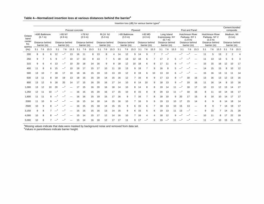
Table 4—Normalized insertion loss at various distances behind the barrier a

Insertion loss (dB) for various barrier typesb

Precast concrete

Plywood

Post and Panel

Cement-bonded composite

I-695 Baltimore (6.7 m)

Distance behind

barrier (m)

I-95 NY (4.9 m)

Distance behind

barrier (m)

I-78 NJ (2.5 m)

Distance behind

barrier (m)

Rt.24 NJ (5.3 m)

Distance behind

barrier (m)

I-95 Baltimore (3.3 m)

Distance behind

barrier (m)

I-83 MD (4.3 m)

Distance behind

barrier (m)

Long Island Expressway, NY

(6.7 m) Distance behind

barrier (m)

Hutchinson River Parkway, NY 1

(1.9 m) Distance behind

barrier (m)

Hutchinson River Parkway, NY 2

(3.3 m) Distance behind

barrier (m)

Madison, WI (3.1m)

Distance behind

barrier (m)

Octave band

center fre-

quency (Hz) 3.1 7.6 15.3 3.1 7.6 15.3 3.1 7.6 15.3 3.1 7.6 15.3 3.1 7.6 15.3 3.1 7.6 15.3 3.1 7.6 15.3 3.1 7.6 15.3 3.1 7.6 15.3 3.1 7.6 15.3

200 8 6 6 12 —a 13 16 11 8 13 8 4 14 12 9 14 9 7 7 —a —a —a — 11 5 13 2 2 4

250 9 7 5 9 —a 10 17 13 8 13 7 5 18 13 12 18 6 7 17 2 5 —a —a — 11 13 13 5 6 3

315 9 6 4 13 —a 10 20 18 14 16 9 8 18 12 10 18 6 8 17 11 6 —a —a — 15 15 16 12 10 17

400 11 8 6 15 —a 10 19 17 15 17 10 11 18 13 9 18 7 9 16 8 5 —a —a — 14 15 15 8 10 12

500 13 10 7 18 17 10 18 16 15 19 13 13 19 12 8 19 6 10 13 10 6 —a —a — 15 16 13 11 11 14

630 13 11 8 19 19 13 18 15 15 20 14 15 16 12 7 16 8 9 17 13 8 —a 18 16 13 16 13 12 13 16

800 13 12 9 18 20 14 17 15 16 20 16 17 14 10 8 14 10 9 18 13 9 —a 19 16 11 16 14 8 10 16

1,000 13 12 10 20 —a — 17 15 16 20 16 18 14 10 8 14 8 8 19 14 11 —a 18 17 10 13 12 13 14 17

1,250 12 11 10 —a —a — 16 15 15 20 16 17 15 10 8 15 8 8 20 13 11 —a 18 16 8 11 10 14 16 17

1,600 11 11 9 —a —a — 16 16 15 19 15 17 16 9 7 16 7 8 18 10 9 20 17 15 8 10 10 14 17 17

2000 11 10 9 —a —a — 16 15 14 18 14 15 16 10 7 16 9 9 19 13 10 17 15 14 8 9 8 14 18 14

2500 10 9 8 —a —a — 16 15 15 18 14 15 15 9 6 15 6 7 18 13 10 15 13 — 8 9 7 14 19 17

3,150 9 8 7 —a —a — 15 15 15 16 13 14 15 9 6 15 5 6 19 13 11 13 —a — 9 10 7 14 21 20

4,000 10 8 8 —a —a — 15 14 15 17 12 14 16 10 7 16 4 4 18 12 9 —a —a — 10 11 8 17 22 19

5,000 10 8 7 —a —a — 15 14 16 18 12 17 17 11 9 17 —a 6 19 —a 11 —a —a — 11 —a 10 15 21 21

aMissing values indicate that data were masked by background noise and removed from data set. bValues in parentheses indicate barrier height.

11

A-Weighting of Insertion and Transmission Losses To approximate the sound heard by the normal human ear, A-weighting was applied to the normalized insertion and transmission losses. The A-weighted sound level, in dBA units, is the sound pressure level in decibels measured with a frequency-weighting network corresponding to the A-scale specified by ANSI S1.4–1971 (ANSI 1987). The A-scale tends to suppress lower frequencies, that is, <1,000 Hz. A-weighting relative responses by frequency are listed in Table 6.

The A-weighting factors are applied to the third-octave band levels predicted in the absence of the barrier and to the levels

corrected with the barrier. The A-weighted levels are loga-rithmically summed to produce overall A-weighted levels with and without the barrier. After converting the sound levels (Lp) into sound pressure using

102ref

2 10 pLpp = (10)

sound pressures (p) were added together, then converted back to sound pressure level (SPL) using

)log(10SPL 2ref

2 pp= (11)

to obtain the overall A-weighted sound pressure level. The A-weighted level predicted without the barrier was sub-tracted from the A-weighted level corrected with the barrier to determine a single value for the transmission loss and insertion loss at each distance. The A-weighted insertion losses were normalized in a similar fashion used in each band except that the correction factor was calculated at 550 Hz and added to the A-weighted insertion loss. Predic-tions at 550 Hz best approximate A-weighted sound levels (FHWA 1978a).

The A-weighted normalized insertion and transmission losses are presented in Table 7. These are the final results of the acoustic effectiveness study of this research project. The tabulated values are the A-weighted normalized insertion

Table 5—Transmission loss of barriers a

Transmission loss (dB)

Precast concrete barrier Plywood barrier Glulam barrier Post and panel barrier Octave band

center frequency

(Hz) I-695

Baltimore I-95 NY

I-78 NJ

Rt. 24 NJ

I-95 Baltimore

I-83 MD

I-495 DC

Rt.7 NY

Long Island Express, NY

Hutchinson River Park-way, NY 1

Hutchinson River Park-way, NY 2

200 17 17 11 14 11 —a 14 14 15 —a —a

250 16 19 13 15 13 10 20 16 —a —a 12

315 19 20 16 18 15 13 19 17 —a 16 14

400 19 20 16 21 14 13 21 15 —a —a 14

500 20 21 15 22 14 13 21 14 —a 15 14

630 20 21 16 23 14 16 21 17 —a 15 15

800 19 22 17 23 15 16 21 18 —a 14 15

1,000 19 24 16 23 16 16 22 18 —a 15 14

1,250 19 24 17 21 17 14 22 19 —a 16 15

1,600 18 24 17 22 17 14 22 22 —a 16 15

2,000 18 24 18 24 18 14 21 22 —a 15 15

2,500 17 23 17 24 18 13 20 25 —a 14 13

3,150 17 22 17 22 18 12 19 27 —a 13 15

4,000 17 —a 15 20 18 11 18 26 —a —a 15

5,000 18 —a 16 18 20 12 19 28 —a 15 17 aMissing values indicate that data were masked by background noise and removed from data set.

Table 6—A-weighting relative response by frequency

Frequency (Hz)

A-weighting response

Frequency (Hz)

A-weighting response

200 −100 1,250 0.6

250 −8.6 1,600 1.0

315 −6.6 2,000 1.2

400 −4.8 2,500 1.3

500 −3.2 3,150 1.2

630 −1.9 4,000 1.0

800 −0.8 5,000 0.5

1,000 0.0

12

losses for the three receiver locations and the A-weighted transmission losses for each barrier.

Experimental Error Calculations The experimental error calculation used in this project fol-lows the guidelines established in the standard ANSI S12.8 (ANSI 1987). The method calculates experimental error by summing the variances produced by background noise, differences in the sound levels with and without barriers, errors in the prediction model, and measurement errors. Experimental error is defined as the standard deviation.

The variances of pre-barrier background noise at reference and receiver locations as well as the variance of the differ-ence between the sound levels at the reference and receiver locations were zero, because the receiver sound levels were calculated from the reference sound levels and no back-ground noise influenced the recordings of the reference microphone. For post-barrier conditions, there was no back-ground noise for the reference microphone, but background noise sometimes affected the receiver microphone. The variance of the calculated background noise level was in-cluded if background noise influenced the recordings. Be-cause reference and receiver recordings for the post-barrier conditions were in the two separate cuts for each barrier, the variance of the difference between these two values were included in the error calculations. Bias errors caused by the prediction model and microphone calibration were calcu-

lated, assuming a confidence level of 95%. Conservatively, the calibrator had a bias error of 0.5 dB and the prediction model a bias of 1 dB. At the 95% confidence interval, the bias errors were reduced to variances of 0.06 and 0.25 dB.

The mean standard error values, as well as the range and coefficients of variation of the standard error values, are presented in Table 8. Tabulated values are for the three insertion loss calculations and the transmission loss calcula-tions. Table 8 further breaks down the standard error by showing the errors in calculations affected by and those not affected by background noise.

The standard error calculations provided a measure of the reliability of the insertion and transmission loss data and calculated results. The maximum errors calculated indicate that the error can be ±2 dB even though all the means oc-curred around 1dB. The range of the standard error values did not vary much between calculations, with or without background noise.

Comparison of Normalized and Estimated Insertion Losses A major concern was whether the normalization process for height, distance, and topography for the tested barriers had an overpowering effect on the estimated insertion losses; that is, whether the normalization correction factors had a

Table 7—A-weighted normalized a insertion and transmission losses

Insertion loss (dBA) at distance behind barrier

Barrier type Barrier location

Barrier height

(m)

Distance from road to barrier

(m) 3.1 m 7.6 m 15.3 m

Transmission loss (dBA) at 3.1 m

behind barrier

Precast concrete 1-695, Baltimore, MD 6.7 9.0 12 10 7 19

Precast concrete 1-95, New York City 4.9 6.6 18 17 12 22

Precast concrete 1-78, New Jersey 2.5 10.9 19 16 16 17

Precast concrete Rt. 24, Whippany, NJ 5.3 9.8 19 14 14 22

Plywood 1-95, Baltimore, MD 3.3 2.4b 17 12 8 15

Plywood 1-83, Maryland Weigh Station 4.3 24.4 7 6 7 14

Glued-laminated 1-495, Washington, DC 5.1 1.5b 15 11 7 21

Glued-laminated Route 7, Troy, NY 2.5 4.9 16 14 10 20

Wood post and panel Long Island Expressway, NY 6.7 12.2 18 11 7 15

Wood post and panel Hutchinson River Parkway, NY 1 1.9 7.6 21 18 15c 15

Wood post and panel Hutchinson River Parkway, NY 2 3.3 14.0 12 14 12c 15

Cement-bonded composite panel

Madison, WI 3.1 12.2 13 10 15 —d

aNormalized to a height of 4.3 m, a distance 9.2 m from the roadway, and a flat site. bThese barriers were 6.1 m from centerline of outside driving lane. cOver-normalized. dTransmission loss data not collected.

13

significant impact on the estimated insertion losses, making the normalized insertion losses more of a prediction than a measurement. Visual comparison of the graphs of the esti-mated and normalized insertion losses suggested that, for the most part, normalization only slightly affected the insertion losses. The normalization process only had a significant effect on the results from barriers where the topography shortened their effective height or from the barrier situated on top of an earth berm.

The conditions that necessitated significant normalization occurred with the two Hutchinson River Parkway wood post and panel barriers and the I-78 New Jersey precast concrete barrier. One Hutchinson River Parkway barrier was only 1.9 m high and was situated 7.6 m from the road. At 15.3 m behind the barrier, the insertion loss was 6 to 15 dB across the 200- to 5,000-Hz range of frequencies. When compared with the predicted insertion loss of 13 to 20 dB at the same receiver location across the same range of frequencies for a 4.3-m-high barrier 9.2 m from the road, the normalization correction factor ranged from 5 to 11 dB. The site of the other Hutchinson River Parkway barrier slopes downward from the roadway, then upward beyond the barrier. This valley effectively reduces the height of the barrier. For the 3.3-m-high barrier situated 14.0 m from the road, the nor-malization correction factors ranged from 0 to 6 dB, with only the 4,000- and 5,000-Hz frequencies escaping a correc-tion factor. The precast concrete barrier on I-78 New Jersey was the only barrier in this study for which an earth berm forms part of the barrier. Although the barrier is only 2.5 m high, it rests on an approximately 1.7-m-high earth berm, which increased its insertion loss. Comparing the perform-ance of this barrier with that of the Route 24 New Jersey

precast concrete barrier, it is clear that the insertion losses differed for the same design. By normalizing the results for the earth berm, the insertion loss of the I-78 barrier was reduced 2 to 3 dB across the entire range of frequencies. In doing so, the insertion losses of the two barriers converged (Table 7).

Aside from these three instances, normalization of the inser-tion losses had only a minimal effect. For the most part, the normalization correction factor only applied to frequencies less than 1,000 Hz. At the receiver position 15.3 m behind the barrier, the data for some barriers required normalization correction factors at frequencies slightly greater than 1,000 Hz, but these were usually about 1 or 2 dB. Thus, because A-weighting suppresses levels below 1,000 Hz, most normalizations did not affect the final A-weighted insertion losses. Except for the Hutchinson River Parkway barriers and the I-78 New Jersey barrier, the normalization correction factors for the A-weighted sound levels were less than 3 dB, a change in sound level that is barely perceptible to the normal human ear.

Trends Within Design Types Acoustic trends occurred within the different design types. The A-weighted insertion losses in Table 7 allowed com-parisons of the insertion losses for different barrier design types. The same data allowed comparison of the perform-ance of each barrier to a target minimum insertion loss of 10 dBA at 3.1, 7.6, and 15.3 m behind the barrier. The results presented as the A-weighted transmission loss in Table 7 allowed comparison of the transmission losses produced by each barrier.

Table 8—Standard errors for insertion and transmission loss calculations

Standard errors for data taken at various distances behind barriers, with and without background noisea

w/back no back w/back no back w/back no back w/back no back

(3.1 m) (3.1 m) (7.6 m) (7.6 m) (15.3 m) (15.3 m) (TL) (TL)

Receiver location

Mean (dB) 1 1 1 1 1 1 1 1

Max. (dB) 2 2 2 2 2 2 2 2

Min. (dB) 1 1 1 1 1 1 1 1

COV (%) 7 7 9 8 10 9 6 5

Receiver location group meansb

Mean 1 dB 1 dB 1 dB 1 dB

COV (%) 7 9 10 5 aw/back designates data affected by background noise; no back, data not affected by background noise; TL, transmission loss. bStandard error means and COVs for insertion losses at each receiver location and transmission losses. Means and COVs include data sets affected and unaffected by background noise.

14

The precast concrete barriers generally had fairly high inser-tion losses (7 to 19 dBA) for the three receiver positions. A large portion of the data for the barrier on I-95 outside New York City was masked by background noise. These data, consequently, were not considered reliable. However, for the other precast concrete barriers, insertion loss was between 12 and 19 dBA at 3.1 m behind the barrier, between 10 and 16 dBA at 7.6 m, and between 7 and 16 dBA at 15.3 m. Even though the values range widely, they can be used as minimum and maximum values for the following reasons. At greater distances (7.6 and 15.3 m) from the barrier, an inser-tion loss of 15 dBA is difficult to achieve. A slight inflation of the values could be due to a slightly different ground effect than predicted. Moreover, the values of 7 and 10 dBA were low for the geometries of the I-95 New York barrier. Thus, the insertion losses of 7 and 10 dBA should also be considered extreme. An insertion loss falling between these two sets of values should be easily attainable. A precast concrete barrier, with a height of 4.3 m and constructed 9.2 m from the road, can attain insertion losses of 16 or 17 dBA at 3.1 m behind the barrier, 13 or 14 dBA at 7.6 dBA, and 11 or 12 dBA at 15.3 m. All these values suggest that the goal of 10-dBA insertion loss is easily at-tainable with precast concrete barriers.

The noise attenuation results for the two plywood barriers were extreme (7 to 17 dBA) near the barrier (3.1 m) and converged to 7 to 8 dBA at the furthest distance (15.3 m) (Table 7). The values at 3.1 and 7.6 m resulted because the I-95 barrier was located directly next to the road and the I-83 barrier was located at least 24.4 m from the road. The farther the barrier is situated from the road, the smaller the insertion loss. Transmission losses for plywood barriers were lower than those for the concrete barriers and may have reduced the insertion losses of the plywood barriers. The low trans-mission losses of the plywood barriers were caused by cracks that had developed between the panels or the panels and posts and by the low surface mass density of the 1.92-cm-thick plywood. Increasing the number of plywood layers or plywood thickness and paying careful attention to details to avoid cracks should raise the transmission loss such that transmission through the barriers should not affect the insertion loss. With these adjustments, the 10-dBA minimum insertion loss for plywood barriers can be achieved.

Insertion losses for glued-laminated barriers were 15 and 16 dBA at 3.1 m, 11 and 14 dBA at 7.6 m, and 7 and 10 dBA at 15.3 m behind the barriers (Table 7). These re-sults suggest that the insertion loss goal of 10 dBA is attain-able by glued-laminated barriers. The transmission losses for the glued-laminated barriers were in close agreement (20 and 21 dBA). These values are plausible because of the thick (6.67-cm) glued-laminated panels used in these barriers. The 10-dBA insertion loss can be obtained without an adverse effect from noise traveling through the barrier.

In contrast, the post and panel barriers offered the most divergent set of noise attenuation results (Table 7). Several reasons can account for the variable results. Background noise masked some data from the 1.9-m-high Hutchinson River Parkway barrier, providing incomplete results. In addition, both Hutchinson River Parkway barriers were influenced by high correction factors in the normalization process. Consequently, the attenuation results should not be used to make final decisions about post and panel barriers but imply that higher attenuation values are possible. The other post and panel barrier, on Long Island Expressway, had insertion loss values of 18 dBA at 3.1 m, 11 dBA at 7.6 m, and 7 dBA at 15.3 m, and a transmission loss of 15 dBA. By improving the detailing of the barrier, both the transmission and insertion losses can be improved. Thus, post and panel barriers have attainable insertion losses of 15 or 16 dBA at 3.1 m, 13 or 14 dBA at 7.6 m, and 10 dBA at 15.3 m. Therefore, the insertion loss goal of 10 dBA is also attainable by post and panel barriers.

The transmission loss values for post and panel barriers were also masked by background noise. Available data converged to a transmission loss of approximately 15 dBA. The low transmission loss caused an insertion loss of 10 dBA to decrease by about 2 dBA. This low value was a consequence of poor detailing of these barriers. The tongue and groove panels pulled apart or the panels were separated from the posts. In either case, gaps that allow sound to travel through the barrier are avoidable with proper detailing. Because dimension lumber contains enough mass to produce a suffi-cient transmission loss, careful detailing should increase the transmission loss of post and panel barriers to values greater than 15 dBA.

Comparison of Design Types The insertion and transmission losses of the different design types allowed comparison of noise attenuation. Comparisons were made among wood barriers and between wood and concrete barriers.

Most of the A-weighted insertion losses reported in Table 7 satisfied the 10-dBA minimum insertion loss goal. The only barrier that did not satisfy this goal at 3.1 and 7.6 m behind the barrier was the I-83 plywood barrier. The insertion losses suffered from the lengthy distance between this barrier and the road/sound source. Because insertion loss at a constant receiver location behind the barrier decreases as the distance between the sound source and barrier increases, the insertion losses of the I-83 barrier at the three receiver locations were less than the 10-dBA insertion loss goal. The insertion losses at 15.3 m behind the barrier averaged 12 dBA for the precast concrete and post and panel barriers and 10 dBA for the plywood and glued-laminated barriers. One precast concrete barrier, the I-695 barrier, did not satisfy the 10-dBA inser-tion loss goal. The plywood barriers on I-83 and I-95 suf-fered from acoustic leaks and low surface mass density that can be corrected by careful detailing; that is, the poor

15

performance should not be attributed to the material. Thus, all insertion losses of the I-83 plywood barrier and the inser-tion loss at 15.3 m behind the I-95 barrier did not satisfy the insertion loss goal of 10 dBA. The only glued-laminated barrier that did not satisfy the 10-dBA insertion loss goal was the I-495 barrier. The post and panel on the Long Island Expressway also suffered from acoustic leaks, causing an insertion loss of 7 dBA at 15.3 m behind the barrier, well below the insertion loss goal. The two Hutchinson River Parkway barriers, however, suffered from “over normaliza-tion” as a result of their geometries, causing insertion losses of 15 and 12 dBA, well above the insertion loss goal. Thus, the insertion losses, determined from the in situ measure-ments presented here for the Route 7 glued-laminated barrier and Hutchinson River Parkway post and panel barriers were similar to the losses for the I-95, I-78, and Route 24 concrete barriers. All these barriers satisfied the 10-dBA insertion loss goal at 3.1, 7.6, and 15.3 m behind the barrier. The I-695 concrete barrier, the I-95 and I-83 plywood barriers, the I-495 glued-laminated barrier, the Madison cement-bonded composite panel, and the Long Island Expressway post and panel barrier had similar insertion losses. These barriers that did not satisfy the 10-dBA insertion loss goal as a result of detailing, low surface mass, and large distances between sound source and barrier.

The average transmission loss for the four concrete barriers and two glued-laminated barriers was 20 dBA. For the two plywood barriers and three post and panel barriers, the aver-age transmission loss was 15 dBA. The values for the con-crete and glued-laminated barriers were high enough to have little impact on the insertion losses. The low values for the plywood barriers were caused by the low surface mass of plywood. Poor detailing also contributed to low transmission loss values for the plywood barriers as well as the post and panel barriers. The panels pulled apart to create gaps, which can be avoided through proper detailing.

Public Acceptance Public acceptance of the various types and designs of sound barriers focused on the public perception of visual compati-bility. This involved asking individuals to evaluate com-puter-edited images of sound barriers using a series of rating scales. This testing allowed for a wide variety of design choices to be narrowed down so that general design guide-lines for barriers could be established.

Selection of Design Types The computer-generated images, which were presented in 35-mm slides, were designed for evaluation of the general appearance of wood barriers rather than the appearance of specific barrier design types. This was done because the casual observer cannot distinguish between plywood, timber, and glued-laminated barriers, whether viewed from the residential or highway side. This is particularly the case

when the highway side is viewed from a fast-moving car. Thus, the images varied in barrier layout and panel orienta-tion rather than finish or detail.

Variations of barrier layout were a flat or linear plan, relief plan, and shadowbox plan (Fig. 4). In the flat plan, the posts and panels were centered on a single line. In the relief plan, the posts were centered on a single line and the panels were connected in two ways: (1) alternately to the front and back of the posts or (2) alternately front-to-front and back-to-back of the posts. The shadowbox plan was similar to the relief plan except that additional panels were installed to deepen the relief. Panel orientation considered variations in the elevation of the barriers. Variations included wide and nar-row strips, horizontal and vertical strips, and combinations of these strips (Fig. 5).

All variations in barrier layout and elevation were developed after reviewing designs of existing barriers. Given the wide variety of designs, the objective was to include most of the feasible barrier designs in the public acceptance evaluation.

To compare the public acceptance of various wood barriers as opposed to concrete barriers, slides of precast concrete barriers were created, using the three layout variations and standard wide horizontal panels. For example, slide F11 showed a barrier constructed of wide horizontal panels in the relief plan layout, viewed from the front or highway side. A matrix of the various barrier designs was developed for comparing the wood and concrete barriers (Table 9). A total of 36 slides was used for the evaluation; in half the slides, the barrier is viewed from the front and in the remainder, from the back.

Slides Modeling All slides for the public acceptance evaluation were created using an IBM compatible personal computer. Different types of barriers were modeled using AutoCAD Release 12 (Autodesk, Inc., San Rafael, California).

Figure 4—Barrier layout plans for public acceptance evaluation.

16

The models were created as three-dimensional objects, which were then rendered by imposing texture, color, and lighting. Each model included three or four bays of the barrier. To ensure that panel orientation and width were distinguishable, strips were placed between panels, creating recesses that created shadows between panels when the model was rendered with a light source. The models were then placed in two views with perspectives similar to those of two background slides. At the same time, two general light sources were imposed on the model to simulate sunlight, illuminating the side facing the viewer.

Rendering To render the models, the rendering menu in AutoCAD was replaced by the Autovision package by Autodesk (Autodesk, Inc., San Rafael, California). This package allowed for colors and textures to be scanned from slides of existing barriers and applied to the models. The scanned colors and textures were saved as a targa (.tga) file, which is acceptable as a texture file by Autovision. This texture file was manipu-lated within Autovision to adjust material properties such as reflectivity and roughness. The file was then applied to the AutoCAD model. Care was taken to ensure that the grain of the texture was parallel with the orientation of the panel or post. Finally, the barrier was rendered using the raytracing method and saved as a targa file.

Figure 5—Panel orientation variations for public acceptance evaluation.

Table 9—Matrix of barrier designs for public acceptance evaluation a

Barrier type

Panel orientation and size Flat Relief

Shadow box

Vertical, wide strips F1 / B1 F2 / B2 F3 / B3

Horizontal, narrow strips F4 / B4 F5 / B5 F6 / B6

Vertical, narrow strips F7 / B7 F8 / B8 F9 / B9

Horizontal, wide strips F10 / B10 F11 / B11 F12 / B12

Vertical and horizontal F13 / B13 F14 / B14 F15 / B15

Concrete F16 / B16 F17 / B17 F18 / B18

aNumbers are codes that identify the slides; F and B refer to front (highway) side and back (residential) side of the barrier, respectively. These letters were then applied to each box in the matrix, which had a number.

17

Creating The goal was to create slides of barriers that appeared as realistic as possible. Each computer-rendered image was imported into the image-editing program PhotoStyler (Aldus Corp., Seattle, WA) and superimposed on a background slide. Using the barrier in the background slide, the bright-ness, contrast, perspective, and size of the rendering were adjusted to match the rest of the slide. The rendering was then copied, pasted, and enlarged or reduced to cover the barrier in the slide. The top edge of the barrier was sharp-ened and the bottom edge was blended with the landscape to create the appearance that the barrier actually belonged in the slide. The finished slide was saved for importing into a presentation program. The end result of the photography, modeling, rendering, image editing, and formatting was 36 slides of barriers, including views from both the highway and residential sides. Reproductions of these slides are presented in Appendix B and are labeled with the codes presented in Table 9.

Testing Setup The 36 computer-edited slides were used to evaluate the appearance of highway sound barriers. Twenty-four study participants rated the 36 slides using semantic-differential (SD) rating scales and individual rating scales. The participants were divided into three groups of eight each. Each group rated all 36 slides using the SD scales and a select group of slides using the individual rating scales. The SD and individual rating scales were used in separate ses-sions to limit the time of each session and so maximize the ability of the participants to concentrate on the scales. Within each session, the slides were divided into two sets: barriers viewed from the highway side and those viewed from the residential side. Each study group was first pre-sented with the highway-side views and asked to rate the barriers from the perspective of a driver. After a 5-min break, each group was presented with the residential-side views and asked to rate the barriers from the perspective of a homeowner living next to the barrier. The goal was to de-termine if varying perspectives would result in different ratings.

The study participants included undergraduate students, graduate students, and staff members from Pennsylvania State University, as well as people employed elsewhere in State College, Pennsylvania. The students were from throughout the United States and the world, including Guate-mala, France, Canada, Venezuela, Australia, and India. The participants ranged from 20 to 40 years of age; the majority were 25 to 30. All study groups were read the same set of instructions, given the same set of forms to read and sign, and presented with the same examples of sound barriers and the same set of slides.

Figure 6—Example of semantic-differential scales used for public acceptance evaluation.

Semantic-Differential Rating Scales The SD scales were used for the first evaluation session. These scales have been used successfully in the evaluation of subjective responses to lighting systems (Flynn 1977) and for other aspects of the built environment (Rohles 1971). The SD scales consisted of a set of bipolar adjectives and a seven-point rating scale; example SD scales are presented in Figure 6. A response closest to the adjective on the left was given a rating of 1 and a response closest to the adjective on the right a rating of 7. If neither adjective described or was applicable to the barrier, a rating of 4 was recorded.

The SD scales were designed to elicit specific responses to attributes of various barrier designs. The scales were an attempt to identify all the factors involved in an opinion about a sound barrier design. The responses were statisti-cally analyzed to determine how many factors influenced them and which barrier attributes caused these responses. The numbers on the scales were not included on the test instrument and were later incorporated as reference codes for analysis. For example, the acceptable/unacceptable rating scale was designated scale 5 (Fig. 6).

(1)appropriate :____:____:____:____:____:____:____: inappropriate

(2)pleasant :____:____:____:____:____:____:____: foreboding

(3)confining :____:____:____:____:____:____:____: spacious

(4)attractive :____:____:____:____:____:____:____: unattractive

(5)acceptable :____:____:____:____:____:____:____: unacceptable

(6)intimidating :____:____:____:____:____:____:____: inviting

(7)imposing :____:____:____:____:____:____:____: unimposing

(8)satisfactory :____:____:____:____:____:____:____: unsatisfactory

(9)gloomy :____:____:____:____:____:____:____: cheerful

(10)darkening :____:____:____:____:____:____:____: lightening

(11)bright :____:____:____:____:____:____:____: dim

(12)dreary :____:____:____:____:____:____:____: cheerful

(13)distinctive :____:____:____:____:____:____:____: ordinary

(14)offensive :____:____:____:____:____:____:____: unoffensive

(15)distracting :____:____:____:____:____:____:____: focusing

(16)appealing :____:____:____:____:____:____:____: unappealing

(17)interesting :____:____:____:____:____:____:____: uninteresting

(18)safe :____:____:____:____:____:____:____: unsafe

(19)fortifying :____:____:____:____:____:____:____: weakening

(20)secluded :____:____:____:____:____:____:____: exposed

(21)private :____:____:____:____:____:____:____: public

(22)cluttered :____:____:____:____:____:____:____: uncluttered

(23)rural :____:____:____:____:____:____:____: urban

(24)harmonious :____:____:____:____:____:____:____: clashing

(25)environmentally environmentally friendly :____:____:____:____:____:____:____: hostile

18

Principal component factor analysis and analysis of covari-ance (ANCOVA) were used to determine which scales were used in a consistent manner and what was the statistical significance of the results. (The statistical analyses and their results are explained in the section on analysis of rating scales.) The results of the SD scales were also used to select slides for evaluation by individual rating scales. The slides selected were those that drew favorable responses on the SD scales for both the highway and residential perspectives. For comparison purposes, the concrete barriers that received the most favorable responses and the most unfavorable re-sponses were used for the individual ratings.

The ratings were converted into points (rating 1 = 1 point, rating 2 = two points, etc.), resulting in 20,700 responses.

Group means were computed for each slide and response. The resulting values are listed in Tables 10–12 for the highway-side views and in Tables 13–15 for the residential-side views. These values were then analyzed using principal components factor analysis. This analysis determined the number of factors that caused the variance between slide ratings. Even though many factors may have been involved in causing the variance, it was usually possible to determine a few factors that explained a majority of the variances. When the factors and the scales that constitute these factors were identified, the scales that made up each factor for each subject were averaged. The averaged results for each factor and slide were then subjected to an ANCOVA to determine if variations between the averaged results were statistically significant.

Table 10—Semantic-differential scale mean results of sound barriers viewed from highway side, group 1

Mean rating for various barrier designsa

Scale F1 F2 F3 F4 F5 F6 F7 F8 F9 F10 F11 F12 F13 F14 F15 F16 F17 F18

1 3.63 4.38 3.63 3.13 3.25 5.38 4.00 3.75 4.38 3.00 3.25 4.25 3.75 3.63 4.88 4.13 3.25 3.75

2 4.13 3.88 4.13 3.13 4.00 5.25 3.50 3.25 4.75 3.00 3.25 4.25 3.38 3.38 4.75 4.00 3.38 4.00

3 3.25 3.75 3.13 3.88 4.13 3.63 4.00 4.13 3.88 4.38 4.25 3.25 4.13 3.50 3.75 3.88 4.13 4.38

4 3.63 3.88 3.75 3.25 3.25 5.38 4.13 3.75 4.00 3.25 2.88 4.13 3.88 3.38 5.00 4.63 3.75 4.13

5 3.00 3.50 3.75 3.00 2.75 5.50 3.38 3.00 3.88 2.75 2.75 4.00 3.25 3.25 4.38 3.63 3.00 3.63

6 4.25 4.13 3.63 4.00 3.13 1.88 3.63 4.00 2.75 3.88 4.50 3.00 4.25 4.00 3.38 3.88 4.13 3.13

7 4.13 4.13 3.50 4.38 2.63 1.63 3.63 4.00 2.88 3.25 4.25 3.00 4.25 3.38 3.38 4.25 3.75 3.13

8 2.88 3.38 3.63 3.13 3.38 5.38 3.38 3.13 4.13 3.00 2.63 4.00 3.50 3.50 5.00 3.63 3.25 3.63

9 3.75 3.75 3.00 3.88 4.00 3.00 4.13 4.00 3.25 3.63 4.88 3.38 3.88 4.00 3.13 3.50 4.38 3.75

10 3.00 2.88 2.88 4.00 2.75 2.50 4.63 3.13 2.75 3.25 4.00 3.50 3.75 2.88 2.75 5.00 5.00 4.88

11 5.00 4.63 4.88 4.38 4.75 5.38 3.88 4.63 5.00 4.38 3.75 4.50 4.25 4.50 5.38 2.75 2.75 2.75

12 3.50 3.25 3.63 3.63 3.75 2.88 4.00 3.38 2.88 3.50 4.00 3.38 3.63 3.75 2.88 4.00 4.13 3.88

13 3.38 4.50 2.25 3.25 2.63 2.38 3.38 3.25 1.75 3.38 3.88 2.88 3.38 2.75 2.75 5.38 3.75 3.13

14 4.88 4.50 4.25 4.63 4.50 2.50 4.75 4.50 3.63 4.63 5.00 3.88 4.50 4.25 3.38 4.50 4.50 3.88

15 3.50 3.75 3.38 4.00 3.75 2.13 3.13 3.50 2.13 4.00 3.63 3.13 3.75 3.00 2.63 4.88 5.00 3.75

16 3.50 4.13 3.63 3.50 3.50 5.25 3.88 3.25 3.75 3.25 2.88 4.00 3.63 2.88 5.00 3.75 3.50 3.88

17 3.38 4.13 2.88 3.13 3.25 3.38 3.50 3.63 3.13 3.50 3.00 3.25 4.00 2.50 4.13 5.13 3.63 3.13

18 3.50 3.13 3.38 2.50 2.50 4.13 3.13 3.13 3.13 2.88 3.38 2.63 3.25 3.00 3.63 2.63 2.13 2.50

19 3.50 3.38 2.38 3.13 2.75 2.13 3.25 3.25 2.38 3.13 2.88 2.38 3.38 2.63 2.88 2.88 1.75 1.63

20 3.88 3.13 3.13 3.38 4.50 3.25 3.63 3.38 3.50 3.25 3.38 3.38 3.63 3.25 3.25 4.25 3.75 3.75

21 3.75 4.00 3.63 3.75 3.25 3.38 3.50 3.88 3.25 3.50 3.38 3.38 3.63 3.13 3.63 4.88 4.00 4.63

22 4.63 4.38 4.38 4.38 5.25 2.63 4.13 4.25 2.50 5.38 4.50 3.13 3.75 4.25 3.25 5.50 4.13 3.88

23 4.13 4.25 4.13 4.38 4.63 3.38 4.13 4.13 4.25 3.13 3.63 4.63 3.63 4.50 3.75 5.25 6.25 5.38

24 4.63 4.13 4.00 3.50 4.25 5.50 4.00 4.38 4.38 3.38 3.63 4.00 4.25 3.25 5.00 4.38 4.25 4.38

25 4.25 3.63 3.63 3.75 3.13 5.25 4.00 3.75 3.88 3.38 3.25 4.13 3.75 3.25 4.5 4.13 4.75 4.50

aSee Table 9 for description of barriers.

19

Individual Rating Scales Fourteen of the 36 slides rated by the SD scales were se-lected for evaluation by individual rating scales. These slides were shown again to the study groups, who were asked to rate the barriers on the basis of their own personal criteria. The individual rating scales were aimed at obtaining an overall impression of the barriers and the SD scales at ob-taining subjective impressions of specific areas.

The individual rating scales were quite simple. Participants were asked to rate each design on a scale from 1 to 10, with the rating relative to all the other designs shown. As for the SD scales, this procedure was repeated twice, once for the barriers viewed from the highway side and once for those viewed from the residential side.

Analysis of covariance was used to determine the statistical significance of differences between averaged ratings of groups. The individual ratings evaluated slides of wood barriers that had been rated favorable on the SD scales and, for comparison, slides of concrete barriers that had received the most and least favorable ratings. The ANCOVA deter-mined whether the differences between favorable and unfa-vorable ratings, and between ratings for wood and concrete barriers, were statistically significant. Thus, the individual rating scales served as a check of the findings obtained by the SD scales. If the responses of the individual rating scales reinforced the findings of the SD scales, then the SD scales were given more validity. If the individual rating scales and SD scales did not show the same trend, it was inferred that the SD scales did not identify the correct responses or factors involved in personal evaluation of barrier designs.

Table 11—Semantic-differential scale mean results of sound barriers viewed from the highway side, group 2

Mean rating for various barrier designsa

Scale F1 F2 F3 F4 F5 F6 F7 F8 F9 F10 F11 F12 F13 F14 F15 F16 F17 F18

1 3.75 3.13 4.00 4.25 4.88 5.00 4.13 4.00 4.25 3.75 3.50 4.38 3.75 3.88 4.88 4.00 4.13 4.88

2 4.13 3.00 4.25 4.13 4.88 5.38 3.98 3.63 4.63 3.88 3.88 4.88 3.88 4.25 5.25 3.88 4.13 4.88

3 4.13 4.50 3.50 4.13 3.63 3.13 4.50 4.88 3.63 4.00 4.25 3.13 3.50 3.63 3.25 4.75 4.25 4.00

4 4.50 3.38 4.38 4.63 5.38 4.75 3.88 4.25 5.00 4.00 3.63 4.75 4.25 4.38 4.88 3.88 4.00 5.25

5 4.13 3.00 4.25 4.13 4.88 5.00 4.13 3.88 4.00 3.88 3.50 4.75 4.50 4.00 4.75 3.75 3.88 4.63

6 4.00 4.38 3.50 4.00 3.63 3.50 4.00 4.50 3.75 4.00 3.88 3.13 4.00 4.00 3.13 3.50 3.75 3.63

7 4.00 4.63 3.25 3.75 4.00 3.38 4.00 3.88 3.50 3.88 3.88 3.13 3.75 4.00 3.38 3.63 3.63 2.75

8 4.25 3.25 4.38 4.00 4.88 4.88 3.88 3.75 4.13 3.88 3.25 4.88 4.25 4.00 5.13 3.88 4.13 4.63

9 4.25 3.63 4.25 4.00 3.13 2.50 4.25 4.63 3.13 3.88 3.88 3.25 3.25 3.38 2.75 4.38 4.63 3.25

10 4.25 3.13 3.88 3.88 2.25 1.88 4.50 4.88 2.75 3.00 3.75 3.25 3.13 3.38 2.50 5.63 5.75 5.63

11 4.50 4.63 4.00 4.38 5.25 5.63 3.63 3.63 4.88 4.75 4.00 4.50 4.88 4.50 5.25 3.00 3.13 3.13

12 4.25 4.13 3.88 3.63 3.00 2.75 4.38 4.25 3.25 4.25 4.00 3.13 3.25 3.75 3.00 4.25 4.25 3.63

13 4.88 3.75 3.13 4.00 3.13 2.50 4.13 4.13 3.13 3.75 4.13 3.13 4.63 4.00 3.38 5.25 4.75 4.25

14 4.88 4.88 4.25 4.13 3.75 2.50 4.25 4.50 3.63 4.63 5.00 3.38 3.88 4.13 4.50 4.25 4.38 3.38

15 4.38 3.75 3.75 3.88 4.00 3.38 3.88 3.75 3.75 4.13 4.13 4.00 4.25 3.88 3.75 4.00 4.13 4.00

16 4.38 3.50 4.13 4.25 4.50 4.63 4.13 3.88 4.63 3.88 4.00 4.75 4.88 4.25 4.75 4.25 4.38 5.00

17 4.75 3.50 4.00 4.38 3.88 4.00 4.00 4.38 3.50 4.50 4.13 3.88 4.50 4.38 3.88 3.88 4.25 3.88

18 4.00 3.38 4.00 2.88 3.13 4.00 3.50 2.88 3.00 3.13 2.75 2.88 4.00 3.50 3.88 2.75 2.50 2.75

19 4.13 3.13 3.63 2.75 3.00 2.63 3.13 3.00 3.00 3.25 3.00 2.38 3.75 3.25 3.13 2.38 2.00 2.25

20 4.13 3.88 3.50 3.88 3.63 3.50 3.88 3.63 3.38 3.75 4.25 3.75 3.88 3.13 3.63 4.00 3.88 4.13

21 4.38 3.63 3.38 4.38 3.38 3.25 4.38 4.13 3.00 3.50 3.63 3.63 3.75 3.88 3.63 4.38 4.50 3.75

22 4.63 3.88 3.63 4.00 3.50 3.25 4.50 4.25 3.75 4.75 4.75 3.63 3.75 3.38 3.38 4.88 4.63 3.88

23 4.38 4.13 4.25 4.88 4.63 5.25 5.25 5.13 4.00 3.38 4.38 4.75 3.25 3.50 3.88 6.13 5.88 5.88

24 3.75 3.25 5.00 4.00 4.13 4.63 4.25 4.25 4.13 3.88 3.50 4.50 4.00 3.75 4.50 4.38 4.00 4.63

25 3.88 3.00 4.50 4.38 4.25 4.63 4.13 4.00 3.50 3.75 3.25 4.25 3.88 4.00 4.00 4.38 4.13 4.63

aSee Table 9 for description of barriers.

20

The slides for individual rating included highway and resi-dential views of seven barrier designs: F2/B2, F4/B4, F6/B6, F10/B10, F11/B11, F13/B13, and F17/B17. Slides F2/B2, F4/B4, F10/B10, F11/B11, and F13/B13 received favorable responses for both the highway and residential sides. Slides F6/B6 received the most negative responses, and slides F17/B17 of the concrete barrier design received the most favorable responses. Results of individual rating by slide and study participant are presented in Table 16. An analysis of variance (ANOVA) was performed on the means and indi-vidual values to determine the statistical significance of differences between the group responses and among the results.

Analysis of Rating Scales Principal Components Factor Analysis of Semantic-Differential Ratings The group averages of the SD scales for each slide were subjected to a principal components factor analysis (Flynn and others 1979). This analysis statistically determined the subsets of rating scales that were used in similar or consis-tent ways by the study participants. A group of scales evalu-ated in a consistent manner had high intercorrelation; that is, consistent rankings of alternatives resulted in high intercor-relation. Strong differences in individual ratings of factors were not required. When the mean values of the ratings were

Table 12—Semantic-differential scale mean results of sound barriers viewed from the highway side, group 3

Mean rating for various barrier designsa

Scale F1 F2 F3 F4 F5 F6 F7 F8 F9 F10 F11 F12 F13 F14 F15 F16 F17 F18

1 4.29 3.43 4.86 4.43 4.71 5.00 5.29 5.14 4.29 4.29 4.29 4.57 4.14 4.57 4.71 4.71 5.29 5.00

2 4.57 3.14 4.86 4.29 5.00 5.00 4.86 5.29 4.14 4.57 4.43 4.57 4.57 4.57 4.86 5.57 5.57 5.29

3 3.43 3.57 2.86 3.43 2.86 2.57 3.14 3.57 3.43 3.00 3.14 3.43 3.29 3.14 3.29 2.71 2.71 3.00

4 4.86 3.43 4.57 4.57 4.86 5.14 5.14 5.57 4.29 4.86 4.57 4.29 4.57 4.57 5.00 5.86 5.57 6.00

5 4.14 3.14 3.86 4.14 4.43 4.71 4.86 5.00 3.71 4.00 4.00 4.00 3.86 4.14 4.29 4.57 4.29 5.43

6 3.43 4.00 3.43 3.71 3.00 2.43 3.43 3.29 4.00 3.29 3.4,3 3.14 3.57 3.57 2.86 2.57 2.71 2.29

7 3.57 4.57 3.00 3.43 2.86 2.14 2.71 2.71 3.57 3.29 3.86 3.29 3.43 3.29 3.14 2.43 2.43 2.14

8 4.29 3.14 4.29 4.14 4.43 5.00 4.57 5.14 3.86 4.29 4.29 3.43 4.29 4.71 4.29 4.57 4.57 4.71

9 3.57 4.14 3.29 3.14 2.71 2.57 3.86 3.71 3.00 3.14 3.43 3.29 3.00 3.00 2.57 3.14 3.29 3.14

10 3.57 3.71 3.57 3.00 2.14 2.14 3.86 3.86 2.86 3.00 3.29 3.00 3.00 2.57 2.29 4.71 4.86 4.86

11 3.86 4.14 4.29 4.86 5.29 5.00 4.00 4.14 5.00 4.86 4.43 4.29 4.71 5.29 5.14 3.29 3.00 3.00

12 3.29 4.29 3.14 3.29 3.00 2.43 3.71 3.29 3.29 3.00 3.29 3.57 3.14 2.86 2.71 3.29 3.29 3.00

13 3.71 3.43 3.29 4.29 3.29 2.86 3.86 3.57 2.86 4.71 4.00 3.29 4.14 4.14 3.14 5.43 5.43 3.86

14 3.57 4.71 3.57 3.14 2.86 3.14 2.71 3.00 4.00 3.14 3.43 3.86 3.14 3.57 3.57 2.86 3.29 2.43

15 3.29 4.14 2.86 3.43 2.86 2.57 2.43 2.14 3.14 3.00 3.14 3.14 3.14 .3.29 2.57 3.57 3.14 2.14

16 4.43 3.57 4.43 5.00 4.86 5.43 5.43 5.43 4.29 5.00 4.36 4.29 4.57 4.86 4.86 5.86 5.43 5.86

17 4.43 3.86 3.71 5.14 4.29 4.14 4.29 4.57 3.43 4.86 4.29 3.86 4.71 4.71 4.00 5.71 5.29 5.29

18 3.57 3.86 3.71 3.43 3.71 3.43 4.29 4.14 3.29 3.14 4.00 4.00 3.86 4.00 3.57 3.14 3.43 3.43

19 3.57 3.29 3.14 3.14 3.14 2.71 4.00 4.00 2.86 3.29 3.43 2.86 3.29 3.29 3.00 2.86 2.71 2.71

20 4.57 3.29 3.86 2.86 3.57 3.57 4.29 4.29 3.14 3.14 3.43 3.43 3.71 3.29 3.57 3.71 5.57 4.43

21 4.14 3.00 3.86 3.71 3.43 4.00 4.43 4.29 3.00 3.00 3.43 3.29 3.29 3.29 3.71 3.43 4.71 4.14

22 3.43 4.57 3.71 3.57 3.43 3.57 3.43 3.00 3.29 3.57 3.43 3.29 2.71 3.14 2.57 4.86 4.43 2.86

23 4.00 3.00 3.43 3.57 3.57 3.86 4.71 4.86 3.71 3.43 3.57 3.14 3.29 3.57 3.71 5.71 6.29 6.43

24 4.57 3.29 4.43 4.86 4.57 5.43 5.29 5.43 4.29 4.71 4.57 4.29 4.57 5.00 4.86 5.29 5.29 5.71

25 4.14 3.43 4.14 3.71 3.86 4.57 4.14 4.43 4.14 3.86 1 86 3.71 3.57 3.86 3.86 4.43 4.00 4.57

aSee Table 9 for description of barriers.

21

calculated, these factor subsets were plotted so that alterna-tives being tested could be directly compared. Their validity was shown if scales that should have a high intercorrelation consistently ranked alternatives in a similar manner. Reasons for inconsistent rankings must be determined.

The results given in Tables 10 to 15 were analyzed using the principal components factor analysis in the statistical pro-gram Minitab. Seven components, or factors, were computed for both views (highway and residential sides) of the barri-ers. Although the analysis determined all the factors, only the seven factors that caused the most variance between barrier ratings were displayed. This analysis identified the three factors that caused most of the variations, thereby eliminating the need for identifying the remainder of the factors.

The results of the analysis included the loadings that each scale had on each factor. Loadings were values ranging between 1 and –1, with the absolute value of the loading being the measure of intercorrelation. Positive and negative loadings were due to the organization of the terms (adjec-tives) in each SD scale. In some scales, the positive adjective appeared on the left side and in others, on the right side. A negative loading indicated that ratings favored the adjective on the left and a positive loading that ratings favored the adjective on the right. Thus, 0.9 and −0.9 had a high loading of the same value. The loadings for seven factors for barriers viewed from the highway side and residential side are pre-sented in Tables 17 and 18, respectively.

Table 13—Semantic-differential scale mean results of sound barriers as viewed from the residential side, group 1

Mean rating for various barrier designsa

Scale B1 B2 B3 B4 B5 B6 B7 B8 B9 B10 B11 B12 B13 B14 B15 B16 B17 B18

1 3.63 3.63 4.75 3.25 3.63 4.13 2.88 4.13 4.63 3.00 3.13 4.50 3.13 3.75 5.00 4.50 4.75 5.23

2 3.50 3.00 4.75 3.13 4.38 4.38 2.88 3.50 4.63 3.13 3.63 4.63 3.25 3.63 5.00 4.50 4.50 5.38

3 3.75 4.13 3.63 4.00 4.00 3.13 2.88 3.63 3.25 3.00 3.50 3.00 3.38 3.63 3.25 2.50 2.25 3.75

4 3.50 3.63 4.50 3.75 4.50 4.50 3.50 3.50 4.38 3.25 3.25 4.50 3.75 4.00 5.13 4.63 5.00 5.75

5 3.50 3.38 4.50 3.25 3,63 4.00 2.88 3.50 4,38 3.00 2.88 4.13 3.13 3.13 4.88 4.25 4.63 5.38

6 3.38 4.50 3.25 4.38 3.88 3.00 4.25 3.88 3.00 4.25 3.88 2.88 4.38 4.25 2.88 3.25 3.25 2.25

7 3,63 4.63 2.50 4.13 4.13 4.00 4.13 4.13 3.38 3.88 4.00 3.00 4.38 3.75 3.63 3.38 3.00 2.38

8 3.25 3.25 5.00 3.13 3.75 4.00 3.13 3.00 4.25 2.88 3.13 4.13 3.13 3.38 5.13 4.50 4.63 5.13

9 4.00 3.88 3.13 4.00 2.63 3.00 4.63 4.25 3.25 4.00 3.88 3.25 3.88 4.25 3.13 3.63 3.75 3.25

10 4.25 4.00 3.38 4.13 2.50 2.88 4.75 4.50 3.00 3.38 3.88 2.88 4.25 3.88 3.00 5.38 5.25 5.00

11 3.50 4.25 4.50 3.88 5.13 5.00 3.50 3.63 5.00 3.88 4.13 4.75 3.75 4.63 5.00 2.63 2.50 2.88

12 4.00 3.88 3.25 4.13 3.13 3.00 4.50 4.00 3.50 3.75 3.88 3.25 4.25 4.25 3.13 3.75 3.75 3.63

13 4.00 4.25 3.13 3.50 3.88 2.88 2.88 3.63 2.75 3.75 3.00 2.88 3.38 3.38 2.50 3.75 3.50 3.50

14 4.38 5.13 3.25 4.38 3.75 2.88 4.38 4.13 3.88 4.88 4.75 2.88 4.50 4.38 2.88 3.75 3.88 3.50

15 3.50 4.50 3.13 3.88 4.00 3.25 4.00 3.50 3.38 4.25 3.88 3.25 4.00 3.88 2.63 3.63 3.38 3.25

16 3.88 3.25 4.75 3.50 4.50 4.50 3.13 3.63 4.38 3.38 3.63 4.50 3.13 3.00 5.13 4.50 4.88 5.50

17 4.50 4.00 3.75 3.38 4.25 2.75 3.25 3.63 3.50 3.75 3.00 3.38 3.50 3.50 3.50 4.88 4.13 4.38

18 3.75 3.38 2.88 2'.75 3.13 3.00 3.00 2.88 3.13 3.00 2.88 3.00 3.38 2.63 3.38 2.38 2.50 2.50

19 3.50 3.13 2.38 3.13 3.38 2.50 3.13 3.25 3.00 3.38 3.00 2.50 3.13 2.63 2.25 2.00 2.25 2.13

20 3.50 3.00 3.13 3.38 2.88 3.50 3.63 3.50 3.50 2.88 3.38 2.88 3.38 3.00 3.38 3.63 3.63 3.63

21 3.75 3.00 3.13 2.88 2.75 3.38 3.00 3.13 3.38 2.63 3.25 3.25 2.88 2.75 3.00 4.50 4.25 4.38

22 4.38 4.25 3.88 4.38 4.25 4.25 4.13 4.13 3.88 4.25 4.25 3.88 3.63 3.88 3.00 5.13 4.63 3.63

23 3.88 3.13 4.38 3.38 3.50 4.25 3.88 3.75 4.13 2.75 3.50 3.63 2.88 3.00 3.50 5.63 5.50 5.75

24 3.88 2.75 4.38 2.88 3.75 4.00 3.50 3.75 4.63 3.63 3.50 4.13 3.50 3.63 4.50 4.88 5.00 5.63

25 3.38 3.00 4.50 3.25 3.88 3.38 3.38 3.38 4.00 3.75 3.25 4.00 3.63 3.75 3.63 5.38 5.13 5.38

aSee Table 9 for description of barriers.

22

The three factors that caused most variance in the ratings were named for identification purposes as evaluative, envi-ronmental, and physical (Tables 17 and 18). The scales corresponding to emotional responses (such as appropri-ate/inappropriate, pleasant/foreboding, and attractive/ unattractive) were named evaluative. The scales concerned with the effect of the barrier design on the surrounding (such as darkening/lightening, bright/dim, public/private, and rural/urban) were given the name environmental. Finally, the scales concerned with impressions of the personal state of being caused by the barrier design (fortifying/weakening and safe/unsafe) were named physical.

The evaluative, environmental, and physical factors caused 75.7% of the variance in the ratings of the highway-side

views and 76.4% of the variance in those of the residential-side views. These factors were evaluated by the same SD scales from both sides, indicating that the factors were the same for the two sides. Because the remainder of the factors from both views only explained about 4% or less of the variances, the evaluative, environmental, and physical factors were used for the remainder of this analysis and the analysis of variance.

The loadings of the scales on the evaluative, environmental, and physical factors were examined more closely to deter-mine which loadings were significant. Loadings of approxi-mately ±0.7 and greater were considered high. Loadings close to the high limit were judged subjectively. If the loading of a scale was close to the limit and the scale

Table 14—Semantic-differential scale mean results of sound barriers as viewed from the residential side, group 2

Mean rating for various barrier designsa

Scale B1 B2 B3 B4 B5 B6 B7 B8 B9 B10 B11 B12 B13 B14 B15 B16 B17 B18

1 3.75 3.13 4.00 4.25 4.88 5.00 4.13 4.00 4.25 3.75 3.50 4.38 3.75 3.88 4.88 4.00 4.13 4.88

2 4.13 3.00 4.25 4.13 4.88 5.38 3.88 3.63 4.63 3.88 3.88 4.88 3.88 4.25 5.25 3.88 4.13 4.88

3 4.13 4.50 3.50 4.13 3.63 3.13 4.50 4.88 3.63 4.00 4.25 3.13 3.50 3.63 3.25 4.75 4.25 4.00

4 4.50 3.38 4.38 4.63 5.38 4.75 3.88 4.25 5.00 4.00 3.63 4.75 4.25 4.38 4.88 3.88 4.00 5.25

5 4.13 3.00 4.25 4.13 4.88 5.00 4.13 3.88 4.00 3.88 3.50 4.75 4.50 4.00 4.75 3.75 3.88 4.63

6 4.00 4.38 3.50 4.00 3.63 3.50 4.00 4.50 3.75 4.00 3.88 3.13 4.00 4.00 3.13 3.50 3.75 3.63

7 4.00 4.63 3.25 3.75 4.00 3.38 4.00 3.88 3.50 3.88 3.88 3.13 3.75 4.00 3.38 3.63 3.63 2.75

8 4.25 3.25 4.38 4.00 4.88 4.88 3.88 3.75 4.13 3.88 3.25 4.88 4.25 4.00 5.13 3.88 4.13 4.63

9 4.25 3.63 4.25 4.00 3.13 2.50 4.25 4.63 3.13 3.88 3.88 3.25 3.25 3.38 2.75 4.38 4.63 3.25

10 4.25 3.13 3.88 3.88 2.25 1.88 4.50 4.88 2.75 3.00 3.75 3.25 3.13 3.38 2.50 5.63 5.75 5.63

11 4.50 4.63 4.00 4.38 5.25 5.63 3.63 3.63 4.88 4.75 4.00 4.50 4.88 4.50 5.25 3.00 3.13 3.13

12 4.25 4.13 3.88 3.63 3.00 2.75 4.38 4.25 3.25 4.25 4.00 3.13 3.25 3.75 3.00 4.25 4.25 3.63

13 4.88 3.75 3.13 4.00 3.13 2.50 4.13 4.13 3.13 3.75 4.13 3.13 4.63 4.00 3.38 5.25 4.75 4.25

14 4.88 4.88 4.25 4.13 3.75 2.50 4.25 4.50 3.63 4.63 5.00 3.38 3.88 4.13 4.50 4.25 4.38 3.38

15 4.38 3.75 3.75 3.88 4.00 3.38 3.88 3.75 3.75 4.13 4.13 4.00 4.25 3.88 3.75 4.00 4.13 4.00

16 4.38 3.50 4.13 4.25 4.50 4.63 4.13 3.88 4.63 3.88 4.00 4.75 4.88 4.25 4.75 4.25 4.38 5.00

17 4.75 3.50 4.00 4.38 3.88 4.00 4.00 4.38 3.50 4.50 4.13 3.88 4.50 4.38 3.88 3.88 4.25 3.88

18 4.00 3.38 4.00 2.88 3.13 4.00 3.50 2.88 3.00 3.13 2.75 2.88 4.00 3.50 3.88 2.75 2.50 2.75

19 4.13 3.13 3.63 2.75 3.00 2.63 3.13 3.00 3.00 3.25 3.00 2.38 3.75 3.25 3.13 2.38 2.00 2.25

20 4.13 3.88 3.50 3.88 3.63 3.50 3.88 3.63 3.38 3.75 4.25 3.75 3.88 3.13 3.63 4.00 3.88 4.13

21 4.38 3.63 3.38 4.38 3.38 3.25 4.38 4.13 3.00 3.50 3.63 3.63 3.75 3.88 3.63 4.38 4.50 3.75

22 4.63 3.88 3.63 4.00 3.50 3.25 4.50 4.25 3.75 4.75 4.75 3.63 3.75 3.38 3.38 4.88 4.63 3.88

23 4.38 4.13 4.25 4.88 4.63 5.25 5.25 5.13 4.00 3.38 4.38 4.75 3.25 3.50 3.88 6.13 5.88 5.88

24 3.75 3.25 5.00 4.00 4.13 4.63 4.25 4.25 4.13 3.88 3.50 4.50 4.00 3.75 4.50 4.38 4.00 4.63

25 3.88 3.00 4.50 4.38 4.25 4.63 4.13 4.00 3.50 3.75 3.25 4.25 3.88 4.00 4.00 4.38 4.13 4.63

aSee Table 9 for description of barriers.

23

appeared similar to other scales evaluating a factor, the scale was considered as evaluating that factor. If the loading of a scale was close to the limit and the scale appeared dissimilar to other scales evaluating a factor, the scale was considered as not evaluating that factor and was eliminated. For barriers viewed from the highway side, the scales 13, 17, 18, 22, and 25 were eliminated. For barriers viewed from the residential side, the scales 3, 9, 13, 17, 20, 22, and 25 were eliminated. These scales were apparently interpreted in different ways. For example, a positive response to scale 17 (interest-ing/uninteresting) could mean that the barrier is interesting in itself or that it creates an interesting effect on the sur-roundings.

The mean values of scales contributing to the evaluative, environmental, and physical factors were calculated to de-termine whether there were any trends in the responses (Tables 17 and 18). The results are graphed in Figures 7 to 12. Overall, the results were more distinctive for the barriers that received negative ratings than for those that received positive ratings. The negative ratings were consistent for certain barriers, whereas the positive ratings were given to several types of barriers. The group means of the barriers favored by the majority were slightly lowered by unfavorable ratings from a few participants, causing the results to be less distinctive.

Table 15—Semantic-differential scale mean results of sound barriers as viewed from the residential side, group 3

Mean rating for various barrier designsa

Scale B1 B2 B3 B4 B5 B6 B7 B8 B9 B10 B11 B12 B13 B14 B15 B16 B17 B18

1 4.29 3.43 4.86 4.43 4.71 5.00 5.29 5.14 4.29 4.29 4.29 4.57 4.14 4.57 4.71 4.71 5.29 5.00

2 4.57 3.14 4.86 4.29 5.00 5.00 4.86 5.29 4.14 4.57 4.43 4.57 4.57 4.57 4.86 5.57 5.57 5.29

3 3.43 3.57 2.86 3.43 2.86 2.57 3.14 3.57 3.43 3.00 3.14 3.43 3.29 3.14 3.29 2.71 2.71 3.00

4 4.86 3.43 4.57 4.57 4.86 5.14 5.14 5.57 4.29 4.86 4.57 4.29 4.57 4.57 5.00 5.86 5.57 6.00

5 4.14 3.14 3.86 4.14 4.43 4.71 4.86 5.00 3.71 4.00 4.00 4.00 3.86 4.14 4.29 4.57 4.29 5.43

6 3.43 4.00 3.43 3.71 3.00 2.43 3.43 3.29 4.00 3.29 3.43 3.14 3.57 3.57 2.86 2.57 2.71 2.29

7 3.57 4.57 3.00 3.43 2.86 2.14 2.71 2.71 3.57 3.29 3.86 3.29 3.43 3.29 3.14 2.43 2.43 2.14

8 4.29 3.14 4.29 4.14 4.43 5.00 4.57 5.14 3.86 4.29 4.29 3.43 4.29 4.71 4.29 4.57 4.57 4.71

9 3.57 4.14 3.29 3.14 2.71 2.57 3.86 3.71 3.00 3.14 3.43 3.29 3.00 3.00 2.57 3.14 3.29 3.14

10 3.57 3.71 3.57 3.00 2.14 2.14 3.86 3.86 2.86 3.00 3.29 3.00 3.00 2.57 2.29 4.71 4.86 4.86

11 3.86 4.14 4.29 4.86 5.29 5.00 4.00 4.14 5.00 4.86 4.43 4.29 4.71 5.29 5.14 3.29 3.00 3.00

12 3.29 4.29 3.14 3.29 3.00 2.43 3.71 3.29 3.29 3.00 3.29 3.57 3.14 2.86 2.71 3.29 3.29 3.00

13 3.71 3.43 3.29 4.29 3.29 2.86 3.86 3.57 2.86 4.71 4.00 3.29 4.14 4.14 3.14 5.43 5.43 3.86

14 3.57 4.71 3.57 3.14 2.86 3.14 2.71 3.00 4.00 3.14 3.43 3.86 3.14 3.57 3.57 2.86 3.29 2.43

15 3.29 4.14 2.86 3.43 2.86 2.57 2.43 2.14 3.14 3.00 3.14 3.14 3.14 3.29 2.57 3.57 3.14 2.14

16 4.43 3.57 4.43 5.00 4.86 5.43 5.43 5.43 4.29 5.00 4.86 4.29 4.57 4.86 4.86 5.86 5.43 5.86

17 4.43 3.86 3.71 5.14 4.29 4.14 4.29 4.57 3.43 4.86 4.29 3.86 4.71 4.71 4.00 5.71 5.29 5.29

18 3.57 3.86 3.71 3.43 3.71 3.43 4.29 4.14 3.29 3.14 4.00 4.00 3.86 4.00 3.57 3.14 3.43 3.43

19 3.57 3.29 3.14 3.14 3.14 2.71 4.00 4.00 2.86 3.29 3.43 2.86 3.29 3.29 3.00 2.86 2.71 2.71

20 4.57 3.29 3.86 2.86 3.57 3.57 4.29 4.29 3.14 3.14 3.43 3.43 3.71 3.29 3.57 3.71 5.57 4.43

21 4.14 3.00 3.86 3.71 3.43 4.00 4.43 4.29 3.00 3.00 3.43 3.29 3.29 3.29 3.71 3.43 4.71 4.14

22 3.43 4.57 3.71 3.57 3.43 3.57 3.43 3.00 3.29 3.57 3.43 3.29 2.71 3.14 2.57 4.86 4.43 2.86

23 4.00 3.00 3.43 3.57 3.57 3.86 4.71 4.86 3.71 3.43 3.57 3.14 3.29 3.57 3.71 5.71 6.29 6.43

24 4.57 3.29 4.43 4.86 4.57 5.43 5.29 5.43 4.29 4.71 4.57 4.29 4.57 5.00 4.86 5.29 5.29 5.71

25 4.14 3.43 4.14 3.71 3.86 4.57 4.14 4.43 4.14 3.86 3.86 3.71 3.57 3.86 3.86 4.43 4.00 4.57

aSee Table 9 for description of barriers.

24

One tendency was the dislike of the shadowbox plan layout. Except for slide F3, all slides of the shadowbox design received negative ratings. Both views of this barrier design (F3 and B3) needed to receive favorable ratings to consider the design as likely to be accepted by the public. Because B3 received negative ratings, F3 was also grouped with the rest of the shadowbox designs as unfavorable.

Another tendency was the less favorable response towards precast concrete barriers. Among the six slides of concrete barriers (F16 to 18, B16 to 18), only F17 received favorable evaluative responses. For comparison purposes, slides F17/B17 were included in the individual rating scales to check this assumption. Even though the concrete barriers were rated as “bright” and “lightening,” these barriers did not receive more favorable evaluative responses. The con-crete barriers were rated as more “fortifying” and “urban” than the wood barriers. They also received negative

evaluative responses, which indicated that the color of a barrier can only help, but not cause, the barrier to be accept-able. Noting that the only wood barriers rated as “lightening” and “bright” were F7 and B7, this tendency was reinforced. This barrier design did not receive as many positive re-sponses as did some other designs. This study suggests that a light finish on a wood barrier is more favorably received than a darker finish. Therefore, the value of the finish on a wood barrier is a factor that merits additional investigation.

Analysis of Variance of S–D Rating Scales Results from the SD ratings and the principal components analysis were used to determine critical differences in value. The critical differences were determined in two steps. First, the mean of the scales contributing to a factor was deter-mined. Second, these means were subjected to an ANCOVA with post hoc tests to determine which means have critical differences.

Table 16—Individual rating scale results and means

Individual rating for various barrier designsa

Highway sidec Residential sided

Codeb F2 F4 F6 Fl0 F11 F13 F17 B2 B4 B6 B10 B11 B13 B17

2A-1 5 4 3 5 6 4 6 7 2 4 6 6 4 3

2A-2 7 6 4 6 6 5 7 6 5 2 7 4 4 3

2A-3 8 10 1 9 8 3 5 8 8 1 10 9 9 1

2A-4 8 9 7 9 9 6 4 8 4 2 7 6 3 1

2A-5 5 8 1 6 4 2 9 4 8 3 9 7 6 1

2A-6 6 9 1 8 3 3 8 7 8 3 9 5 3 5

2A-7 8 9 3 10 5 6 1 9 7 3 7 6 6 1

2A-8 2 6 5 7 6 8 7 6 5 3 5 8 5 3

2B-1 5 8 9 8 7 4 1 8 7 9 10 7 4 2

2B-2 5 6 3 6 5 5 6 6 7 4 6 7 5 3

2B-3 6 4 3 4 5 7 2 7 4 3 4 5 6 2

2B-4 8 5 10 4 6 4 10 9 7 4 8 4 10 10

2B-5 7 1 1 1 2 2 7 9 2 1 2 2 1 1

2B-6 7 4 5 6 8 9 3 9 3 8 5 7 7 4

2B-7 7 4 4 4 6 8 5 5 5 3 6 7 8 7

2B-8 5 4 4 6 5 6 8 5 7 3 6 7 8 8

2C-1 4 6 1 7 3 5 9 6 5 1 8 3 7 2

2C-2 6 3 1 3 2 3 4 4 5 1 4 3 6 3

2C-3 6 8 5 9 9 7 2 6 5 7 6 6 2 1

2C-4 2 7 1 8 9 4 10 2 8 1 10 9 3 4

2C-5 7 8 4 8 9 6 2 9 5 1 4 6 3 3

2C-6 7 6 2 7 5 4 8 9 7 3 8 9 4 1

2C-7 8 9 4 6 7 5 6 10 5 8 8 6 3 7

2C-8 5 7 7 8 6 6 4 7 6 8 6 4 5 1

Mean 6.00 6.29 3.71 6.46 5.88 5.08 5.58 6.92 5.63 3.58 6.71 5.906 5.08 3.21 aSee Table 9 for description of barriers. bSubject identification code where first number is session number, letter is subject group, and second number is subject number. cSlides of barriers viewed from highway side. dSlides of barriers viewed from residential side.

25

The means of six factors—three critical factors (evaluative, environmental, and physical) for each set of two slides (highway and residential views)—were determined solely to reduce the ANCOVA necessary to analyze the responses. Rather than conducting an ANCOVA for each of the 20,700 individual responses, pooling the results across the six fac-tors reduced the responses to a much more manageable 138 mean values. Because of the high intercorrelation of these six factors, the 138 mean values were a good representation of the important SD scale responses. Therefore, performing an ANCOVA on each of these six factors was a satisfactory way to conduct an ANCOVA across the entire set of SD scale responses.

An ANCOVA was conducted to determine if any mean of a study group was significantly different from the other group means and if any mean of a slide was significantly different from that of the other slides. Because the ANCOVA is an omnibus test, it did not specify which group mean was sig-nificantly different from the others nor did it specify which slide mean was significantly different than the others. It only called attention to significant variations in the results. An F-test was conducted to determine if there was significant variation between the group and slide means at a signifi-cance level of 0.05. A Tukey HSD (honestly significant difference) post hoc test was used to determine significant differences between individual means (Stoline 1981).

Table 17—Semantic-differential scale loadings, highway-side views

Factorsa

Scaleb Evalu-ative

Environ-mental Physical 4 5 6 7

Appropriate/inappropriate −0.914 –0.153 –0.026 –0.094 0.080 0.058 –0.027

Pleasant/foreboding –0.932 –0.142 0.008 0.096 –0.035 0.141 0.098

Confining/spacious 0.729 –0.224 0.141 –0.284 0.252 0.060 0.098

Attractive/unattractive –0.892 –0.304 –0.131 0.068 0.111 0.018 0.027

Acceptable/unacceptable –0.883 –0.183 –0.064 –0.093 0.273 0.109 0.197

Intimidating/inviting 0.801 0.073 –0.349 –0.058 0.282 0.065 –0.133

Imposing/unimposing 0.769 0.135 –0.381 0.023 0.325 0.101 –0.179

Satisfactory/unsatisfactory –0.894 –0.109 –0.047 –0.028 0.244 0.154 0.191

Gloomy/cheerful 0.747 –0.379 –0.027 –0.399 –0.020 –0.140 0.130

Darkening/lightening 0.308 –0.873 0.078 –0.122 0.013 –0.245 0.042

Bright/dim –0.281 0.861 –0.136 0.048 0.133 0.244 0.028

Dreary/cheerful 0.785 –0.412 0.084 –0.219 0.046 –0.076 0.281

Distinctive/ordinary 0.113 –0.685 –0.560 0.286 0.014 –0.200 –0.024

Offensive/unoffensive 0.910 0.045 –0.078 –0.036 0.009 0.174 0.021

Distracting/focusing 0.686 –0.297 –0.153 0.392 0.353 0.192 0.143

Appealing/unappealing –0.889 –0.273 –0.220 0.091 0.048 –0.090 0.077

Interesting/uninteresting –0.427 –0.490 –0.618 0.266 0.034 –0.159 –0.048

Safe/unsafe –0.518 0.330 –0.550 –0.415 –0.027 –0.021 0.119

Fortifying/weakening –0.013 0.215 –0.872 –0.263 –0.137 0.052 –0.013

Secluded/exposed –0.113 –0.682 –0.119 –0.098 –0.466 0.444 0.072

Private/public 0.038 –0.781 –0.097 –0.218 0.014 0.269 –0.370

Cluttered/uncluttered 0.693 –0.368 –0.096 0.289 –0.191 0.107 0.142

Rural/urban –0.032 –0.826 0.353 0.045 0.020 0.147 –0.026

Harmonious/clashing –0.845 –0.226 0.015 –0.127 –0.086 –0.127 –0.176

Environmentally friendly/ environmentally unfriendly

–0.568 –0.414 0.303 –0.200 0.441 –0.009 –0.094

Variance 11.274 5.237 2.430 1.098 1.027 0.684 0.491

Percentage of variance c 45.1 20.9 9.7 4.4 4.1 2.7 2.0 aFactors identified by principal components factor analysis; highlighted items identify high loadings on a factor. bSee Figure 6 for example of scales. cPercentage of the total variance accounted by this factor.

26

Results of the ANCOVA are presented in Tables 19 to 21 for barriers viewed from the highway side and Tables 22 to 24 for barriers viewed from the residential side. Each table presents an ANCOVA for one of the six factors identified by the SD scales. The ANCOVA determined the F-test values for the variations between slides and between participant groups for each slide. Using a significance level of 0.05, the critical F-values for the slides and groups were determined to be 1.65 and 1.45, respectively. Although all factors from both views had significant variations between slides, two factors (the environmental factor for the highway side and the evaluative factor for the residential side) had significant variations between groups. Significant variations between

slides were an expected result of the scales. The scales were designed to help determine which barrier design types were preferred and why they were preferred. With the factors identified by the principal components factor analysis, the individual rating scales were established to test whether or not these factors determined the participant’s overall impres-sion of the barrier designs. At the same time, the individual rating scales were established to test the preliminary design guidelines, which embody the tendencies of the SD ratings. The significant variation between study groups, however slight, was not an expected result and necessitated closer investigation.

Table 18—Semantic-differential scale loadings, residential-side views

Factorsa

Scaleb Evaluative Environmental Physical 4 5 6 7

appropriate/inappropriate –0.928 –0.028 0.050 –0.024 –0.157 0.005 –0.026

pleasant/foreboding –0.955 0.041 0.019 –0.128 –0.016 –0.059 0.068

confining/spacious 0.520 –0.275 –0.196 –0.444 –0.456 –0.089 –0.378

attractive/unattractive –0.928 –0.068 –0.035 –0.110 0.008 0.010 –0.054

acceptable/unacceptable –0.905 –0.072 –0.006 –0.181 –0.214 0.157 0.023

intimidating/inviting 0.862 0.009 –0.182 –0.151 –0.121 0.160 –0.078

imposing/unimposing 0.878 0.147 –0.091 –0.180 –0.111 –0.019 0.051

satisfactory/unsatisfactory –0.900 0.002 0.023 –0.226 –0.166 0.158 0.089

gloomy/cheerful 0.651 –0.585 –0.097 0.256 –0.177 0.178 –0.058

darkening/lightening 0.137 –0.917 0.094 0.225 0.031 0.046 –0.149

bright/dim –0.037 0.880 –0.121 –0.358 –0.123 –0.040 0.066

dreary/cheerful 0.748 –0.542 –0.034 0.153 –0.144 0.145 –0.046

distinctive/ordinary 0.027 –0.612 –0.532 –0.275 0.410 –0.136 –0.164

offensive/unoffensive 0.847 –0.210 –0.076 –0.108 –0.098 0.111 0.180

distracting/focusing 0.733 –0.245 0.053 –0.482 0.090 0.128 0.241

appealing/unappealing –0.942 –0.074 –0.131 –0.101 0.105 –0.062 –0.054

interesting/uninteresting –0.469 –0.376 –0.540 –0.169 0.443 0.140 –0.104

safe/unsafe –0.208 0.441 –0.748 0.180 –0.143 0.123 0.114

fortifying/weakening 0.231 0.295 –0.827 0.161 –0.014 0.186 0.089

secluded/exposed –0.351 –0.551 –0.399 0.146 –0.269 –0.421 0.269

private/public –0.425 –0.692 –0.266 –0.016 –0.279 –0.026 0.153

cluttered/uncluttered 0.466 –0.627 0.170 –0.161 0.276 –0.055 0.334

rural/urban –0.490 –0.762 0.117 –0.126 –0.175 –0.119 –0.002

harmonious/clashing –0.992 –0.154 –0.062 0.154 0.030 0.146 –0.058

environmentally friendly/ environmentally unfriendly

–0.676 –0.411 0.263 –0.080 –0.062 0.466 0.096

Variance 11.576 5.219 2.308 1.143 1.076 0.698 0.572

Percentage of variance c 46.3 20.9 9.2 4.6 4.3 2.8 2.3 aFactors identified by principal components factor analysis; highlighted items identify high loadings on a factor. bSee Figure 4 for example of scales. cPercentage of the total variance accounted by this factor.

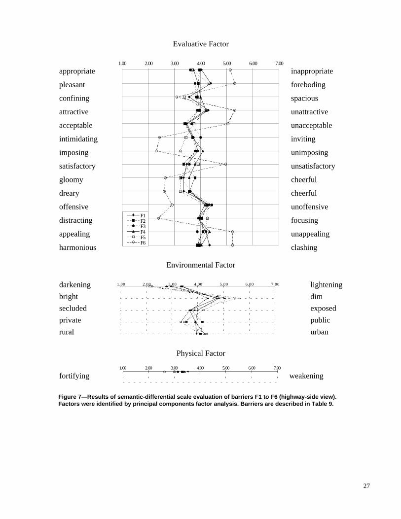
27

Figure 7—Results of semantic-differential scale evaluation of barriers F1 to F6 (highway-side view). Factors were identified by principal components factor analysis. Barriers are described in Table 9.

Evaluative Factor

appropriate inappropriate

pleasant foreboding

confining spacious

attractive unattractive

acceptable unacceptable

intimidating inviting

imposing unimposing

satisfactory unsatisfactory

gloomy cheerful

dreary cheerful

offensive unoffensive

distracting focusing

appealing unappealing

harmonious clashing

Environmental Factor

darkening lightening

bright dim

secluded exposed

private public

rural urban

Physical Factor

fortifying weakening

1.00 2.00 3.00 4.00 5.00 6.00 7.00

F1 F2 F3 F4 F5 F6

1.00 2.00 3.00 4.00 5.00 6.00 7.00

1.00 2.00 3.00 4.00 5.00 6.00 7.00

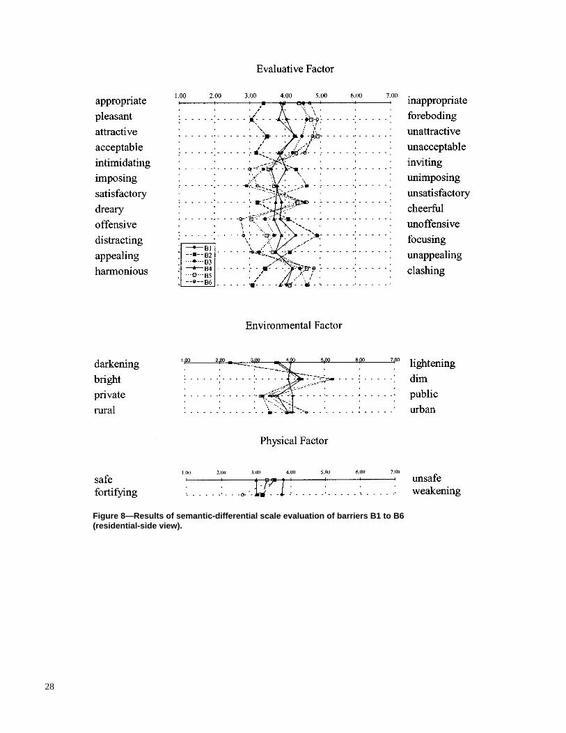
28

Figure 8—Results of semantic-differential scale evaluation of barriers B1 to B6 (residential-side view).

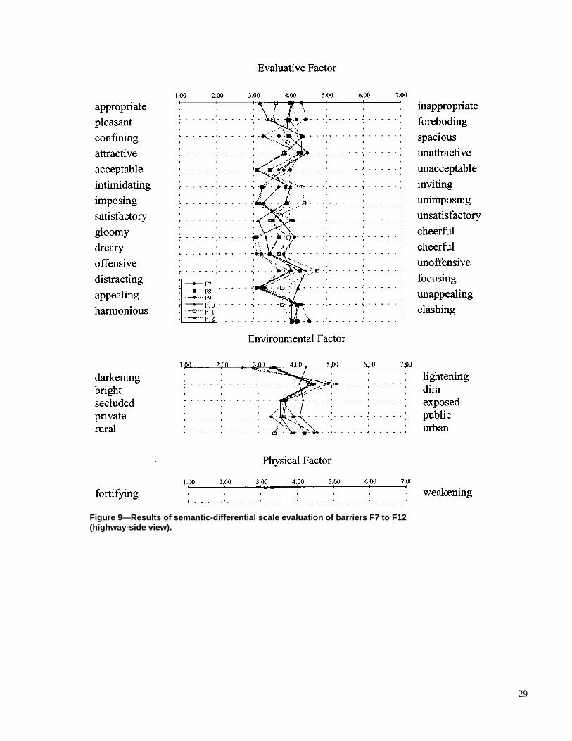
29

Figure 9—Results of semantic-differential scale evaluation of barriers F7 to F12 (highway-side view).

30

Figure 10—Results of semantic-differential scale evaluation of barriers B7 to B12 (residential-side view).

31

Figure 11—Results of semantic-differential scale evaluation of barriers F13 to F18 (highway-side view).

32

Figure 12—Results of semantic-differential scale evaluation of barriers B13 to B18 (residential-side view).

Table 19—ANCOVA of evaluative factor of SD scales, highway-side views a

Result α = 0.05 Source DF SS MS F Fcv

Slide 17 52.958 3.1152 3.25 1.65 Group (Slide) 36 25.3688 0.7047 0.74 1.45 Error 360 344.7105 0.9575

Total 413 423.0374 aDF = degrees of freedom, SS = sum of the squares, MS = means squared, F = ANCOVA F-value, Fcv = critical F-value.

Table 20—ANCOVA of environmental factor of SD scales, highway-side views a

Result α = 0.05 Source DF SS MS F Fcv

Slide 17 123.9796 7.2929 15.02 1.65 Group (Slide) 36 29.3493 0.8153 1.68 1.45 Error 360 174.8107 0.4856 Total 413 328.1396 aDF = degrees of freedom, SS = sum of the squares, MS = means squared, F = ANCOVA F-value, Fcv = critical F-value.

33

The variation between study groups was analyzed with one-way analyses of variance and Tukey post hoc tests to deter-mine which slides had critical F-values and which groups had critical Q-values (also known as T-values). Using a significance level of 0.05, the critical values of F and Q were determined to be 3.49 and 3.58, respectively. With these values, only four values (one ANOVA F-value and three Q-values) showed significant differences. Slide F8, for the evaluative factor, had an F-value of 6.00. The reason for this critical value is the difference between groups 3 and 2, which had a Q-value of 4.93. The other two critical Q-values were for slide B4–environmental factor and slide B7–evaluative factor (Q-values of 3.58 and 3.65, respectively). For slide B4, the critical value appeared in the comparison between groups 1 and 2; for slide B7, the critical value appeared in the comparison between groups 1 and 3. Otherwise, the other F- and Q-values were not significant, indicating that the variance between group means was not significant.

The variations between slide ratings for each factor were analyzed with a Tukey post hoc test. Using a significance level of 0.05, the critical Q-value was determined to be 5.30. The graphs of the results reinforced the tendencies identified in the SD ratings. Barriers that were disliked, such as F6, had more distinctive ratings than barriers that were liked. At best, the positive response to barriers was lukewarm. Again, a

simple plan layout and panel orientation for barriers were favored, and the concrete and shadowbox plans were dis-liked. Thus, we concluded that no significant difference in values was observed between the groups and the preliminary observations can be investigated further with the individual rating scales.

Analysis of Variance of Individual Rating Scales The variation between individual rating scale group means was analyzed using ANCOVA with Tukey post hoc tests. The results of the ANCOVA showed no significant differ-ence between the three study groups, but there was a signifi-cant difference between the slides. The results of the AN-COVA are presented in Table 25 for barriers viewed from the highway side and Table 26 for barriers viewed from the residential side. Each table presents an ANCOVA for indi-vidual ratings from one study group. The ANCOVA deter-mined the F-values for the variations between slides and between study groups for each slide. Using a significance level of 0.05, the critical F-values for the slides and groups were determined to be 2.15 and 1.74, respectively. Although both the residential- and highway-side views showed signifi-cant differences between slides, neither view showed signifi-cant differences between groups.

A Tukey post hoc test was performed on the individual rating scales to determine which ratings were statistically

Table 21—ANCOVA of physical factor of SD scales highway-side views a

Result (α = 0.05)a

Source DF SS MS F Fcv

Slide 17 87.172 5.128 3.51 1.65

Group (Slide) 36 40.451 1.128 0.77 1.45

Error 360 525.375 1.459

Total 413 652.998 aDF = degrees of freedom, SS = sum of the squares, MS = means squared, F = ANCOVA F-value, Fcv = critical F-value. Table 22—ANCOVA of evaluative factor of SD scales residential-side views a

Result (α = 0.05)a

Source DF SS MS F Fcv

Slide 17 67.991 3.999 3.51 1.65

Group (Slide) 36 60.967 1.694 1.49 1.45

Error 360 410.190 1.139

Total 413 539.148 aDF = degrees of freedom, SS = sum of the squares, MS = means squared, F = ANCOVA F-value, Fcv = critical F-value.

Table 23—ANCOVA of environmental factor of SD scales, residential-side views a

Result α = 0.05

Source DF SS MS F Fcv

Slide 17 190.7554 11.2209 19.21 1.65

Group (Slide) 36 13.3569 0.371 0.64 1.45

Error 360 210.317 0.5842

Total 413 414.4294 aDF = degrees of freedom, SS = sum of the squares, MS = means squared, F = ANCOVA F-value, Fcv = critical F-value. Table 24—ANCOVA of physical factor of SD scales, residential-side views a

Result α = 0.05

Source DF SS MS F Fcv

Slide 17 42.691 2.511 1.92 1.65

Group (Slide) 36 41.875 1.163 0.89 1.45

Error 360 470.473 1.307

Total 413 555.039 aDF = degrees of freedom, SS = sum of the squares, MS = means squared, F = ANCOVA F-value, Fcv = critical F-value.

34

significant. This analysis simply determines which differ-ences of means are statistically significant. Results are pre-sented in Tables 27 and 28 for barriers viewed from the highway and residential sides, respectively. In these tables, the column boxhead indicates the mean of the slide being compared. A Q6 indicates the column in which the individ-ual rating of slide F6 or B6, depending on the table, is being compared with the individual ratings of the other slides. The row where the Q-value is located indicates the mean of the other slide being compared.

Some differences in means were statistically significant. The mean response for slide F6 was different from that for slides F2, F4, F10, and F11 (Table 27). The mean responses for slides B6 and B17 were different from the responses for slides B2, B4, B10, and B11 (Table 28). The statistically significant ratings of slides F2/B2, F4/B4, F10/B10, and F11/B11 required that the design tendencies of the barriers illustrated in these slides be embodied in the final design guidelines. The mean responses for slides F13, F17, and B13 were not statistically different from either extreme. Because these means were close to the statistically significant ratings, these three slides helped clarify and reinforce the final de-sign guidelines.

Comparison of Rating Scale Results The results of the SD and individual rating evaluations were combined to observe tendencies that would aid in developing general design guidelines for wood sound barriers. The preliminary guidelines established by the SD scales were the unfavorable response towards concrete and shadowbox designs and the favorable response towards simple designs. By comparing the preliminary guidelines with the results of the individual rating scales, it was possible to determine if the individual rating scales reinforced these guidelines.

The first preliminary guideline was the dislike of the shad-owbox design. This design type received negative responses on both rating scales; the barrier given the most negative ratings was depicted in slides F6/B6. Not only did the study participants dislike the appearance of the shadowbox-type

Table 25—ANCOVA of individual rating scales, highway-side views a

Result α = 0.05

Source DF SS MS F Fcv

Slide 6 98.917 16.486 3.08 2.15

Group (Slide) 14 85.667 6.119 1.14 1.74

Error 147 786.25 5.349

Total 167 970.833 aDF = degrees of freedom, SS = sum of the squares, MS = means squared, F = ANCOVA F-value, Fcv = critical F-value.

Table 26—ANCOVA of individual rating scales, residential-side views a

Result α = 0.05

Source DF SS MS F Fcv

Slide 6 254.952 42.492 8.54 2.15

Group (Slide) 14 56.083 4.006 0.81 1.74

Error 147 731.25 4.974

Total 167 1,042.286 aDF = degrees of freedom, SS = sum of the squares, MS = means squared, F = ANCOVA F-value, Fcv = critical F-value.

Table 27—Tukey post hoc test results for individual rating scales of barriers viewed from highway side (αα = 0.05)a

Slideb Meanc F6d F13 F17 F11 F2 F4 QCVe

F6 3.71

F13 5.08 2.98

F17 5.58 4.06 1.09

F11 5.88 4.72 1.74 0.65

F2 6.00 4.98 2.00 0.91 0.26

F4 6.29 5.61 2.63 1.54 0.89 0.63

F10 6.46 5.98 3.00 1.91 1.26 1.00 0.37 4.22

aBoldface entries indicate significant difference between rating means. bBarriers described in Table 9. cIndividual ratings scale means for slides calculated in Table 18. dQ-value between slide ratings of column label and row label. eCritical Q-value. Table 28—Tukey post hoc test results for individual rating scales of barriers viewed from residential side (αα = 0.05)a

Slideb Meanc B17d B6 B13 B4 B11 B10 QCVe

B17 3.21

B6 3.58 0.83

B13 5.08 4.19 3.36

B4 5.63 5.42 4.60 1.23

B11 5.96 6.16 5.33 1.97 0.74

B10 6.71 7.85 7.02 3.65 2.42 1.68

B2 6.92 8.32 7.49 4.13 2.89 2.15 0.47 4.22

aBoldface entries indicate significant difference between rating means. bSlides defined in Table 9. cIndividual ratings scale means for slides calculated in Table 18. dQ-value between slide ratings of column label and row label. eCritical Q-value.

35

barrier, they found it more “fortifying” than barriers with the same panel elements organized in the flat and relief plan layouts. Thus, shadowbox designs are not recommended for wood sound barriers from an aesthetic viewpoint.

The second preliminary guideline was the negative response towards precast concrete barriers. These barriers were rated as more “fortifying” and “urban” than the wood barriers. By including both views of the only favorably received concrete barrier (slides F17/B17) in the individual rating scales, it was possible to test this hypothesis. The residential-side view of this barrier received an unfavorable response, but the highway-side view received a favorable response. The mean rating for this slide was not statistically different from that of the slide receiving the worst rating nor was it different from that of the slide receiving the best rating. Its value, however, was closer to those of the slides given favorable responses than those given unfavorable responses. Thus, the reason for the somewhat favorable ratings of this concrete barrier needs to be investigated further.

Like the favorably rated designs of wood barriers, the design of the precast concrete barrier was simple. Its wide horizon-tal pattern and simple relief plan were similar to that of a wood barrier given favorable ratings. However, the material properties of concrete apparently led the study participants to give negative ratings to the same barrier viewed from the residential side. The rural background presented in the slides also could have influenced the ratings. The SD scales indi-cated that the concrete barriers were perceived as “urban” and wood barriers were perceived as “rural.” It was possible that the background could have biased the participants against the concrete barriers. Because wood barriers were perceived to have more “rural” qualities than concrete barri-ers, a rural background could have caused the participants to view wood barriers as more acceptable in the setting estab-lished. The fact that one view of a concrete barrier received a favorable rating suggests that there was not a bias against concrete per se. Nevertheless, the remainder of the responses indicated that wood barriers are more likely to be accepted by the public than are precast concrete barriers.

The final preliminary guideline from the SD scales was that the design type should be simple in plan layout and panel orientation. The four barriers given favorable responses in the individual rating scales shared this trait. These barriers were depicted in slides F2/B2, F4/B4, F10/B10, and F11/B11 (Table 9). Even though no one plan or panel layout was favored above the others, the barrier designs shown in slides F13/B13 and F17, which were given ratings close to those of the favored barriers, offered some insight into the preferred design traits. These designs used a simple flat or relief plan layout. Thus, the favorably rated barriers suggest that simplicity is important, not a specific plan layout or panel orientation. The simplicity guidelines, which lead to design guidelines for wood barriers most likely to be ac-cepted by the public, are summarized as follows:

• Simple flat walls with either many or few elements in the elevation or relief walls with few elements in the eleva-tion

• Barriers with many elements or a relief plan layout, but not both, to break up the monotony of long barriers

• Panels with either vertical or horizontal orientation in the elevations

Structural Requirements for Prototype Barrier A systematic design procedure was developed to provide detailed information on the performance of wood barriers. A single prototype barrier was designed and fabricated so that a series of measurements could be conducted under more controlled conditions than was possible for the in situ meas-urements previously discussed. Data on acoustic effective-ness and public acceptance collected during the first phase of this project were applied to the structural requirements and construction details presented here.

Systematic Approach to Design A system of eight wood sound barriers encompassing several design alternatives with similar details was developed. The designs included the details and plan layouts (discussed in the previous sections) that were determined to be acousti-cally effective and aesthetically acceptable. The fundamental design was solid-sawn timber or glued-laminated wood posts with dimensional lumber panels or manufactured glued-laminated panels. This system included three plan layouts and two panel orientations. Each sound barrier can be con-structed according to one post design guideline and two different connection detail guidelines. Posts were selected from a chart that assigns a post size for a given bending and minimum shear stress. Panel materials required a minimum bending stress. Acoustic performance criteria and aestheti-cally acceptable formats obtained from the public acceptance evaluation were incorporated into the design details. The basic system of wood sound barriers was structurally ana-lyzed based on the expected loading and designed accord-ingly.

An initial sound barrier design matrix was developed from several design styles, plan layout, and material options. This matrix, based on wood materials used for sound barriers outlined in the Guide Specification for Wood Highway Noise Barriers (NFPA 1985), consisted of all possible design options, plan layouts, and panel orientations that were under consideration (Table 29).

The matrix was developed to determine the sound barrier designs that could be incorporated into a systematic design approach where one standard set of design details encom-passing acoustic performance and public acceptance could

36

be applied to each design option. No additional aesthetic evaluations were conducted. Individual design options were then ruled out on the basis of (1) the standards set from the acoustic effectiveness and public acceptance evaluations and (2) design details incompatible with a systematic design approach.

In the public acceptance evaluation, the following character-istics were described as aesthetically acceptable for wood sound barriers: simple flat or relief plan layout, many ele-ments with horizontal or vertical alignment in flat format or few elements in relief format, and light in color. Specifically, a sound barrier design option was eliminated by public acceptance evaluation if it had many elements combined with the relief format and was dark in color. As a result, the shadowbox layout, which consisted of vertically and hori-zontally aligned elements and was typically dark in color, was eliminated from further consideration. An incompatible design option was the vertical orientation of panel elements in the relief format. Vertical panel elements required a means of attachment other than the posts, which consisted of purlins strung between the posts. Purlins on the front and back of a barrier were required in the relief format and pre-sented awkward construction and incompatible design de-tails. Thus, relief format options with vertically oriented panel elements were also eliminated from further considera-tion. Plywood had shown poor durability in field inspections and was not selected for additional investigation. The re-maining design options are shown in Table 30 and the corresponding plan layouts in Figure 13.

The final design matrix (Table 30) consisted of all the design options that have common details, allowing for a systematic design approach. Specifically, the posts are the same for any design under equivalent conditions of height, spacing, and geography. The panels do not significantly differ from one configuration to another, and the system requires only two different connection details, one for timber plank and the other for a glued-laminated panel.

Figure 13—Plan layout options.

Considerations The systematic design included detailing to prevent sight lines through the barrier to maintain acoustic performance and those attributes of aesthetic details reported from the public acceptance evaluation. To resist development of sight lines, tongue and groove construction, wood moisture con-tent of less than 12% to 15%, and a light-colored preserva-tive treatment were specified for the panel material. A cross section of a typical tongue and groove dimensional lumber plank is shown in Figure 14a. It is important to ensure a tight fit between planks when attaching them to the posts. Manu-factured glued-laminated panels can also be developed with tongue and groove construction or a similar joinery arrangement such as shiplap and rabbetted to prevent sight lines from developing. The individual elements of the panels can be oriented vertically or horizontally. The elements of vertically oriented panels are edge glued and glued flatwise by layer (Fig. 14b). Horizontally oriented panels are made by sawing a wide glued-laminated beam vertically along the longitudinal axis to form two narrower beams of the same depth (Fig. 14c).

Options

Post and Panel—Posts were the same under equivalent conditions for each design option, and panels were dimen-sional lumber planks or manufactured glued-laminated pan-els. The three plan layouts shown in Figure 13 constituted the final design options. The flat flush format was used for four of the eight design options. Panels were attached to the

Table 29—Original sound barrier design matrix

Flush Relief

Shadow-box

Center-line Flat Flat Skewed

Vertical Timber plank Horizontal

Vertical Glued-laminated Horizontal

Vertical Plywood

Horizontal

Table 30—Final sound barrier design matrix

Flush Relief Flat Flat Skewed

Timber plank Vertical X X

Horizontal

Glued-laminated Vertical X X

Horizontal

Flat flush

Flat relief

Skewed relief

37

Figure 14—Options for panel elements.

highway side of the posts and parallel to the highway in horizontal or vertical alignment. In the flat relief format, the panels were aligned parallel to the highway but were alter-nated on the highway and residential sides of the posts. In the skewed relief option, the posts were slightly rotated with respect to the highway and the panels were alternately at-tached to the highway and residential sides of the posts.

From the final design option matrix, the flat flush plan with horizontally aligned timber planks combined with glued-laminated posts was selected as the test barrier. This sound barrier was structurally analyzed and designed according to the Guide Specifications for Structural Design of Sound Barriers (AASHTO 1989a), the Guide Specification for Wood Highway Noise Barriers (NFPA 1985), and the National Design Specification for Wood Construction (AF&PA 1991).

Connections—The connections were galvanized annularly threaded nails, wood screws, or lag bolts, as shown in Figures 15 to 18. Timber plank panels required either two 20d nails or two 76.2-mm-long wood screws on the end of each plank. Pre-boring the pilot holes made driving the nails and screws easier and helped prevent splitting of the wood. Glued-laminated panels required four 50d or 60d nails or two 127-mm-long, 15.875-mm-diameter lag bolts with washers on each panel end. Edge distances and spacing were at least 19 mm for nails and screws and 38 mm for lag bolts.

Procedure

Posts—The Guide Specifications for Structural Design of Sound Barriers (AASHTO 1989a) recommends the use of the Standard Specification for Highway Bridges (AASHTO 1989b), Section 13, Timber Structures, or the use of an industry-recognized design specification for wood sound barriers. The National Design Specification for Wood Con-struction (AF&PA 1991) was used to design the posts and panels. The posts were designed for flexure as a vertically aligned cantilever beam rigidly fixed at ground level. An alternative method was also considered—a cantilever beam having a maximum moment at a point one-third the depth of embedment below ground level. Even though a larger mo-ment occurred below ground level, as shown in Figure 19, this method was not pursued, because the additional cross section of the concrete foundation was assumed to suffi-ciently increase the moment capacity of the post–pier foundation system.

Loading was based on a unit tributary area symmetrically aligned on the centerline of the post. The wind load was distributed over an equivalent single panel section according to the height and width of a panel section. The end posts were also designed in this manner so they could be compati-ble with the interior posts even though they had only half the tributary area. Serviceability criteria for wood structures were based on considerations of creep resulting from sus-tained load and limiting deflections to reasonable values.

w

1.5 in.

.375 in.

~22 in.

2.25 in.

0.75 in.

~22 in.

2.25 in.

0.75 in.

(a) Tongue and groove timber plank

(b) Vertical glued-laminated panel

(c) Horizontal glued-laminated panel

38

Figure 15—Timber plank horizontal nailed or screwed connection.

Figure 16—Glued-laminated horizontal nailed connection. Nominal 2 in. = standard 38 mm. The deflection limitations for unoccupied vertical structures, such as sound barriers, do not need to be as strict as those for horizontal structures subject to human occupancy. Thus, the AASHTO (1989a) Guide Specifications for the Design of Sound Barriers does not include deflection limitations. In this study, a limitation of l/120 on horizontal deflections was adopted for the design of the posts. This helped keep the posts in the system to a size that could be easily manufac-tured by industry. Figures 20 and 21 display simplified post design charts for solid-sawn timbers with bending stresses of 5.2 MPa and 9.3 MPa, respectively. Figures 22 and 23 dis-play the same type of charts for glued-laminated timbers with bending stresses of 11 MPa and 16.55 MPa, respec-tively. The design charts were developed according to the procedure presented in Appendix C, using the allowable stresses shown in Figures 20 to 23. Post dimensions were readily determined from these charts for a given wind pres-sure and sound barrier height. For most applications, sizes in the range of 172 by 279 mm to 172 by 349 mm were suitable for a glued-laminated post. Solid-sawn posts were typically larger and ranged from 203 by 305 mm to 254 by 356 mm.

Panels—Panels were designed by the action of the wind load on one panel element (plank or glued-laminated panel). The design method consisted of comparing the stress caused by the wind load with the allowable stress of the panel ele-ment. Calculations showed that the allowable stress for bending was much greater than the actual stress caused by the design wind load. In other words, the design wind load did not create significant bending stresses in the panel of the sound barrier. Thus, most common structural wood listed in the National Design Specification for Wood Construction (AF&PA 1991) could be used for the panels. However, the applied stress should always be compared with the allowable bending stress of the material being considered. Therefore, excluding aesthetics, the only factor in determining which quality of panel material to use was its potential for develop-ing sight lines, which would increase sound transmission. A lower grade of wood contains more defects, which have the potential to develop sight lines. For example, No. 1 Southern Pine has fewer knots that may produce holes over time and is more likely to be kiln dried after treating than is No. 2 or No. 3 grade wood, even though those grades have sufficient allowable bending stresses.

Foundations—Several types of foundations can typically be used for post and panel wood sound barriers. These include pier, top collar, spread footing, and continuous spread (trench) footing (Fig. 24).

The pier, top collar, and spread footing foundations were used in the design of the sound barrier system. The trench footing was not considered for design because it could be replaced by the spread footing in most applications, which requires less concrete over the length of the sound barrier.

The pier foundations, which were used in the test sound barrier, were designed using a wind speed of 113 km/h (70 mph) (Exposure B2) in accordance with the Guide Specifications for Structural Design of Sound Barriers (AASHTO 1989a). The calculation procedure to determine foundation depths was based on the method outlined in the 1994 Uniform Building Code (UBC 1994) and the Guide Specifications for Structural Design of Sound Barriers (AASHTO 1989a) and verified by the post-design equations developed by the American Society of Agricultural Engi-neers Subcommittee on Post and Pole Foundations (ASAE 1992). The resulting design is shown in Figure 25. The dimensions depended on the loads used in the design, and a 75.6-mm cover was required. The allowable lateral passive soil strength (S) was estimated for design purposes at 30 kPa/m and the angle of internal friction (φ) at 30°.

Design of Test Sound Barrier Design procedures for each element (posts, foundation, and general connections) were developed for the test sound barrier, but they can be applied to all wood sound barrier design options.

Batten (2 in. Nominal) Lg ~ 1.5 in. S

Le

Lg Le Batten (2 in. Nominal)

S ~ 1.5 in.

39

Figure 17—Timber plank vertical nailed or screwed connection.

Figure 18—Glued-laminated vertical bolted connection.

3 in.

12 in.

Angle bracket

3 x 3 x 1/4 in.

3-3/8 in.

Timber plank T & G 2 in. nominal

4 x 4 in. Purlin

1-5/8 in.

~ 1 in. 1-5/8 in.

3 in.

12 in.

Angle bracket 3 x 3 x 1/4 in.

3-3/8 in.

Glued-laminated panel

4 x 4 in. Purlin

1-5/8 in.

~ 1 in. 1-5/8 in.

40

Figure 19—Post-flexure design diagrams. General Considerations The test sound barrier was detailed with the acoustic effec-tiveness and aesthetic characteristics determined from the first phase of the project. It was also detailed and constructed to provide maximum durability independent of preservative treatment. This included using tongue and groove lumber, using threaded galvanized nails (or wood screws), and pro-viding drainage paths along the bottom of the barrier. Natu-rally occurring sight lines or gaps can develop between planks in the panel over time and will decrease insertion loss. Therefore, the test sound barrier was constructed to provide opportunity to compare its acoustic performance with that of panels with sight lines. This was done by con-structing connections that provided vertical movement of the planks through slots 3.2 mm larger than the thickness of the planks (Fig. 26). Shims were placed between the planks to provide the desired gap thickness. The gaps extended the entire length of the test sound barrier.

Note that the sight lines were not a design detail but a method of testing how gaps between planks affect the

acoustic effectiveness of the test barrier. Development of sight lines between planks over time caused by uneven drying along the width of a plank is a concern in wood sound barriers. A quantitative measure of sight line effects on a full-scale test model provided useful information for the design of a wood sound barrier.

Design Criteria

American Association of State Highway and Transporta-tion Officials (AASHTO)— The Guide Specifications for Structural Design of Sound Barriers (AASHTO 1989a) establishes the following loads to consider in design of sound barriers: loads resulting from wind pressure, seismic occurrences, earth pressure, traffic (impact), and ice and snow, and loads transferred from bridges, guard rails, or retaining walls. Of these loads, only the wind load was considered in this study because the test barrier was built at a location precluding all other live loads. Dead loads to con-sider are the individual weights of the sound barrier ele-ments. The vertical dead loads were considered negligible in determining structural capacity in relation to the horizontal live loads. Exposure B2 of the Uniform Building Code (1994) and a wind velocity of 113 km/h was used to deter-mine the wind pressure for panel, post, and foundation de-sign. Post and panel design and the foundation design are explained in the following sections.

National Design Specification—The Guide Specifications for Structural Design of Sound Barriers (AASHTO 1989a) recommends the use of the Standard Specification for High-way Bridges (AASHTO 1989b), Section 13, Timber Struc-tures, or the use of an industry recognized design specifica-tion for wood sound barriers. The National Design Specification for Wood Construction (AF&PA 1991) was used to design the posts and panels. The posts were designed as a vertically aligned cantilever beam fixed at ground level and based on a unit tributary area of a panel width symmetri-cally aligned on the centerline of the post. The live load was distributed over an equivalent single panel section of 13.00 m2 according to a height of 4.27 m and width of 3.048 m.

The panels were designed by the wind load acting on one plank. This calculation shows that the allowable stress in bending for 38-mm (nominal 2-in.) structural lumber is greater than the required stress caused by the design wind load.

The connections for the test sound barrier consisted of 50.4- by 151.2-mm planks arranged to provide a mechanism for easy insertion of the panel material, as shown in Figure 26. The connections were attached to the posts with 60d annularly threaded galvanized nails. Note that an in-service sound barrier would use the connection details previously developed.

R 2

R 1

Wind load

L d/3

d

Free body diagram

Shear diagram

wL

R 1 R 2

Moment diagram

Mmax = wL2/2 +wLd/3

L = Post height d = Post embedment depth w = Wind load R1 = Soil resistance resultant

R2 = Soil resistance resultant

41

Figure 20—Solid-sawn post design chart for Fb = 750 lb/in 2.

Figure 21—Solid-sawn post design chart for Fb = 1,600 lb/in 2.

Materials and Selection Justification The test sound barrier was constructed with glued-laminated Southern Pine post combination 16F-V5 with dimensions of 171.45 mm by 314.33 mm by 6.7 m. The panel material was No. 1 Southern Pine tongue and groove, with dimensions of 50.8 mm by 152.4 mm by 3.05 m. A 152.4-mm plank width was used to minimize warp and shrinkage, which leads to the development of sight lines. The length of the barrier (24.4 m) was selected to minimize the diffraction of sound waves around the edges of the barrier. Primary structural

design details are presented in Figure 27. Note that half the sound barrier is shown in elevation.

These materials and the flat flush, horizontally aligned tim-ber plank configuration were selected for the test barrier for the following reasons:

• Simplest and most economical to build

• Relatively easy to conduct acoustic tests with sight lines in the panel

Solid-sawn timbers: Fb = 750 lb/in2

0

2

4

6

8

10

12

14

Wind pressure (lb/ft2)

Pos

t hei

ght (

ft)

15 20 25 31 37

12 x 18 in. 10 x 16 in.

8 x 12 in. 8 x 10 in.

6 x 8 in.

Solid-sawn timbers: Fb = 1350 lb/in2

0

2

4

6

8

10

12

14

Wind pressure (lb/ft2)

Pos

t hei

ght (

ft)

15 20 25 31 37

10 x 14 in. 10 x 12 in.

8 x 10 in. 6 x 8 in.

6 x 6 in.

42

Figure 22—Glued-laminated post design chart for Fb = 1,600 lb/in 2.

Figure 23—Glued-laminated post design chart for Fb = 2,400 lb/in 2.

• Able to obtain materials in a timely manner

• Easier to manage than larger (>55.9-cm-wide) glued-laminated panels

Table 31 presents the actual costs incurred in the construc-tion of the test barrier. In addition to the costs of the material and equipment, construction of the barrier required about 40 h of construction time. This resulted in a total construc-tion cost of $10,130 for the 24.4-m-long by 4.27-m-high test barrier. The cost of this barrier was less than $100/m2, which

is competitive with that of precast concrete and masonry. For instance, a Florida Department of Transportation study showed an average cost of $193/m2 for concrete and ma-sonry barriers (Lindeman 1997).

Durability The durability of the test sound barrier was addressed in two ways. First, the members of the barrier were arranged to maximize durability regardless of preservative treatment. In addition to the design details already discussed, the grooves

Glued-laminated timbers: Fb =1600 lb/in2

0

2

4

6

8

10

12

14

Wind pressure (lb/ft2)

Pos

t hei

ght (

ft)

15 20 25 31 37

8-1/2 x 15-1/4 in.

6-3/4 x 13-3/4 in.

6-3/4 x 9-5/8 in. 5 x 8-1/4 in.

5 x 5 -1/2 in.

Glued-laminated timbers: Fb =2400 lb/in2

0

2

4

6

8

10

12

14

Wind pressure (lb/ft2)

Pos

t hei

ght (

ft)

15 20 25 31 37

8-1/2 x 12-3/8 in.

6-3/4 x 11 in.

6-3/4 x 8-1/4 in. 5 x 6-7/8 in.

5 x 5-1/2 in.

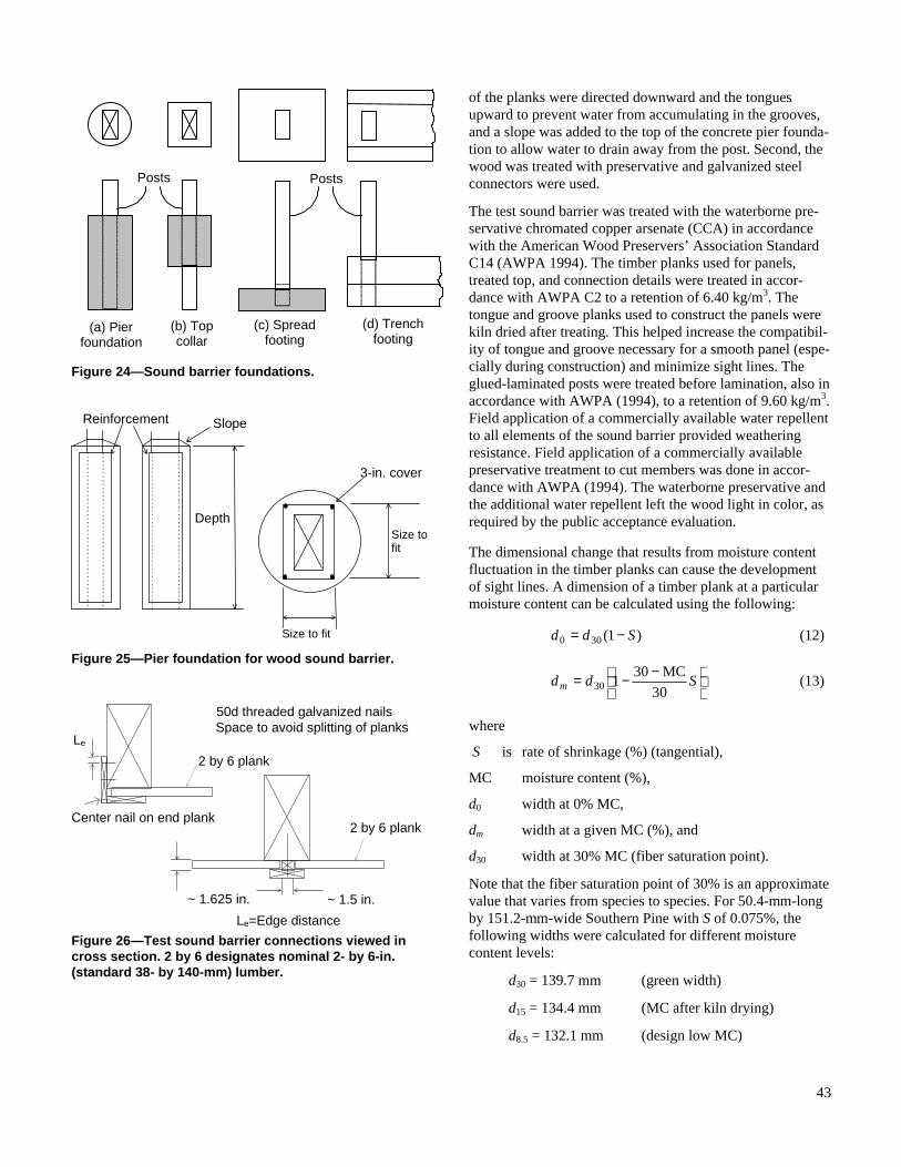
43

Figure 24—Sound barrier foundations.

Figure 25—Pier foundation for wood sound barrier.

Figure 26—Test sound barrier connections viewed in cross section. 2 by 6 designates nominal 2- by 6-in. (standard 38- by 140-mm) lumber.

of the planks were directed downward and the tongues upward to prevent water from accumulating in the grooves, and a slope was added to the top of the concrete pier founda-tion to allow water to drain away from the post. Second, the wood was treated with preservative and galvanized steel connectors were used.

The test sound barrier was treated with the waterborne pre-servative chromated copper arsenate (CCA) in accordance with the American Wood Preservers’ Association Standard C14 (AWPA 1994). The timber planks used for panels, treated top, and connection details were treated in accor-dance with AWPA C2 to a retention of 6.40 kg/m3. The tongue and groove planks used to construct the panels were kiln dried after treating. This helped increase the compatibil-ity of tongue and groove necessary for a smooth panel (espe-cially during construction) and minimize sight lines. The glued-laminated posts were treated before lamination, also in accordance with AWPA (1994), to a retention of 9.60 kg/m3. Field application of a commercially available water repellent to all elements of the sound barrier provided weathering resistance. Field application of a commercially available preservative treatment to cut members was done in accor-dance with AWPA (1994). The waterborne preservative and the additional water repellent left the wood light in color, as required by the public acceptance evaluation.

The dimensional change that results from moisture content fluctuation in the timber planks can cause the development of sight lines. A dimension of a timber plank at a particular moisture content can be calculated using the following:

)1(300 Sdd −= (12)

−−= Sddm 30

MC30130 (13)

where

S is rate of shrinkage (%) (tangential),

MC moisture content (%),

d0 width at 0% MC,

dm width at a given MC (%), and

d30 width at 30% MC (fiber saturation point).

Note that the fiber saturation point of 30% is an approximate value that varies from species to species. For 50.4-mm-long by 151.2-mm-wide Southern Pine with S of 0.075%, the following widths were calculated for different moisture content levels:

d30 = 139.7 mm (green width)

d15 = 134.4 mm (MC after kiln drying)

d8.5 = 132.1 mm (design low MC)

(a) Pier foundation

Posts Posts

(b) Top collar

(c) Spread footing

(d) Trench footing

Reinforcement Slope

Depth

3-in. cover

Size to fit

Size to fit

50d threaded galvanized nails Space to avoid splitting of planks

Center nail on end plank

Le

2 by 6 plank

~ 1.625 in. ~ 1.5 in.

2 by 6 plank

Le=Edge distance

44

Figure 27—Test sound barrier; 14 ft high and 80 ft long.

Therefore, the total width change of one plank was 2.29 mm. According to Equations (12) and (13), a sight line of 4.57 mm can develop between planks with very low mois-ture content. In addition, moisture gradients caused by un-even drying throughout the wood can cause warping (bow, crook, and twist). Crook is the most critical defect because it deforms a plank perpendicular to its edge (strong axis direc-tion), which is in line with the vertical plane of the panel. This will cause gaps to develop between planks.

Acoustic Effectiveness of Test Sound Barrier The acoustic effectiveness of the test sound barrier was determined directly from on-site measurements. The per-formance of the sound barrier was analyzed under three different conditions. The barrier was first tested with sight lines (gaps) between planks. Subsequently, the sight lines

Post, Pier, and Plank Specifications

Posts: Glued-laminated Southern Pine 16F-V5 6-3/4 x 12-3/8 x 22

Pier: Diameter 24 in. Depth 8 ft

CCA Treated (0.60 lb/ft3) Planks: 2 x 6 x 10 tongue and groove

Southern Pine CCA Treated (0.40 lb/ft3)

Notes 1. Place posts and planks allowing for 1.5 in. space on center. 2. Install planks with tongues facing up and grooves facing down. 3. Planks on end panels must be aligned with outer edge of post. 4. Bottom of Barrier must be approximately 6 in. below ground surface. 5. Pier foundations designed for 70 mph wind speed and 10-ft post spacing. 6. Lateral soil pressure (S) of 200 psf/ft and phi = 30 degrees. 7. Align planks with adjacent panels to ground elevation changes.

Nail Schedule

50d Galvanized annular threaded (ring shank) 12-in. spacing on center Space to avoid splitting of planks (3/4-in. edge distance, Le) Prebored pilot holes (1/8-in. bit) Center on edge of face plank on end connectors

Center nail on end plank

Le

Use 50d threaded galvanized nails Space to avoid splitting of planks

~ 1.625 in. ~ 1.5 in.

Reinforcement Slope

3-in. cover

17 in.

10 in.

9.76 ft 10.10 ft typ.

45

were removed and the barrier was tested with and without a treated top. The goals of these tests were to determine actual insertion losses, the effect of sight lines, and the effect of using a treated top. Predictions of the insertion loss of the test sound barrier from test measurements were also made.

Test Procedures

Setup The insertion loss of the test sound barrier was determined according to Methods of Determination of Insertion Loss of Outdoor Noise Barriers (ANSI 1987). This standard speci-fies three methods for determining insertion loss of outside sound barriers: direct measured, indirect measured, and indirect predicted. The direct measured method is recom-mended by the specification and is used when sound meas-urements are taken before the sound barrier is installed. This method was used to determine the insertion loss for the test sound barrier. Insertion loss is the difference between the measured sound pressure levels before and after the sound barrier is installed. The standard (ANSI 1987) requires that the reference and receiver microphones have the same posi-tions and that measurements are taken with equivalent sound source, terrain, ground conditions, and atmospheric condi-tions before and after installation of the sound barrier.

Figure 28—Microphone locations for run 1.

Figure 29—Microphone locations for run 2. The test procedure involved emanation of a steady sound level from a single loudspeaker source and recording of the sound pressure levels at different positions in front, on top, and behind the sound barrier with microphones. Five micro-phones were used at one time; therefore, a set of two runs was made to obtain recordings at each of the eight micro-phone positions. Each microphone was calibrated using a calibrated source with a level of 94 dB at a frequency of 1,000 Hz.

Figures 28 and 29 are elevations of the test configuration for runs 1 and 2. ANSI (1987) requires the use of a reference

Table 31—Cost of materials for test sound barrier

Material Description Cost ($)

Wood Glued-laminated posts (9) 2,913.66

Timber plank panel material (350)

2,446.50

Connectors (9) 75.00

Miscellaneous wood 50.00

Water repellent 390.00

Foundations Reinforcement (3 & 5) 90.00

Concrete (7.25 yd3) 380.63

Augering holes (9) 740.00

Nails and screwsa 2d common nails

16d common nails

16d annular threaded nails

60d annular threaded nails

Wood screws (3-½ in.) 50.00

Crane service 295.00

Equipment purchase 200.00

Equipment rental 500.00

Total cost 8,130.79 aGalvanized.

Source

6 7 8

1.22 m typ.

4.6 m 4.6 m

30.48 m

3

1.37 m

1

1.0 m

4.6 m

Reference microphone

Receiver microphones

1.22 m

2 4 5

5.6 m

0.3 m

1.37 m

3

1 Source

1.0 m

4.6 m

Reference microphone

Receiver microphones

0.3 m

46

microphone in position 3 where the sound from the source can be measured with minimum effects from the sound barrier. In the tests, the source microphone (microphone 1) measured the sound pressure level emitted from the source. Average wind velocity and temperature readings were moni-tored for each run. The point source was positioned 7.62 m (25 ft) in front of the sound barrier for each test. Also, the reference microphone remained 1.37 m above the top and at the center of the barrier for all tests. For run 1, the micro-phones were set at 15.24, 22.86, and 30.48 m behind the barrier. For run 2, the microphones were set at 4.6 m in front and 0.30 and 7.62 m behind the barrier.

Runs 1 and 2 lasted approximately 11 min each. The first 10 min recorded sound from the source, which was used for analysis, and the last minute recorded ambient sound levels with the source off. Run 2 immediately followed run 1 in each set.

Each receiver microphone (2, 4 to 8; Figs. 28 and 29) received 10 min of noise for each data set. The source mi-crophone (1) and reference microphone (3) received 20 min of noise for each data set because they were used for both runs 1 and 2. Ten data sets were obtained for three condi-tions: no barrier (before the barrier was installed), barrier installed with gaps, and barrier installed without gaps. Each data set was divided into five 2-min intervals of recorded noise. An average sound level for the 2 min was determined for each third-octave band. Thus, there were 50 data points for each third-octave band for the no barrier condition and for each of the three barrier configurations: with sight lines (gaps), without gaps and no treated top, and without gaps and with treated top.

Instrumentation Power to the instrumentation was supplied by a portable generator located approximately 30 m from the barrier. The receiver microphones were battery powered. The random noise generator supplied a signal that went through the filter, then to the speaker. An oscilloscope was used to monitor the incoming signal in real time from the receiver microphones. This signal was amplified before being recorded on the cassette recorder. The signal was recorded on cassette tape at a speed of 19 cm/s. Figure 30 displays the instrumentation setup used to conduct acoustical tests, and Table 32 lists the acoustical equipment used.

Site Plan The site plan of the test sound barrier is shown in Figure 31. There were potential outside sound sources with direct paths to the receiver side of the barrier. Specifically, noise from the test track or road and reflection of sound waves off the metal shed may have had an effect on the measured sound pressure levels at the receivers.

Figure 30—Schematic of instrumentation setup.

Table 32—Acoustical testing equipment

Equipment Manufacturer or type Model

no.

Portable power generator

Honda (gasoline) (1,000 W)

Random noise generator

General Radio Company (2 Hz–20 kHz)

1381

Filter Krohn-Hite 3342 Speaker JBL (EON) (15 in.) Source microphone power supply

Two channel 2807

Microphone battery power supply

Brüel Kjear 2810

Oscilloscope BK Precision (20 mHz) 2120 Cassette data recorder TEAC 7 channel MR–30 Amplifier ITHACO 453 Microphones Brüel Kjear ½-in. condenser Sound level calibrator Brüel Kjear (94 dB, 1,000 Hz) 4230

Testing Sequence The sound pressure levels normalized by the sound pressure levels measured by the source microphone were used to determine insertion loss for the sound barrier with and with-out gaps. Measurements of sound pressure levels taken before the sound barrier was installed were used to deter-mine insertion loss. The posts were installed at the time of testing and were considered to have no effect on sound propagation. The before-installation measurements were made in the same season as the measurements made with the barrier in place.

The test sound barrier was first constructed with sound leaks made by systematically inserting six 3.18-mm-wide gaps between the planks in the lower, middle, and upper regions of each panel; the gaps extended the entire length of the barrier (Fig. 32). This allowed testing of approximately 0.5% of the panel area with direct sound propagation through the barrier.

Source microphone

Power supply

All other microphones

Power supply (battery)

Filter

Speaker Random noise

generator

Oscilloscope

Amplifier

Cassette recorder

47

Figure 31—Site plan for test sound barrier.

Figure 32—Locations of gaps in test sound barrier.

1/8-in.-wide gap

14 ft

2 ft 0.85 ft

2 ft 0.85 ft

6.5 ft

6.5 ft

80.9 ft

Posts

Plank interface

9.5 ft 10 ft typ

80 ft

~ 80 ft

Grove of trees

Source microphone

Reference microphone

~ 10 ft

Metal shed

Sound barrier

Test track

North

Distance from barrier (microphone number)

100 ft (8)

75 ft (7)

50 ft (6)

25 ft (5)

1 ft (4)

15 ft (2)

22 ft (1)

0 ft (3)

Road

~ 80 ft

- NTS -

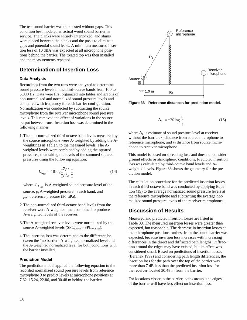
48

The test sound barrier was then tested without gaps. This condition best modeled an actual wood sound barrier in service. The planks were entirely interlocked, and shims were placed between the planks and the posts to eliminate gaps and potential sound leaks. A minimum measured inser-tion loss of 10 dBA was expected at all microphone posi-tions behind the barrier. The treated top was then installed and the measurements repeated.

Determination of Insertion Loss

Data Analysis Recordings from the two runs were analyzed to determine sound pressure levels in the third-octave bands from 100 to 5,000 Hz. Data were first organized into tables and graphs of non-normalized and normalized sound pressure levels and compared with frequency for each barrier configuration. Normalization was conducted by subtracting the source microphone from the receiver microphone sound pressure levels. This removed the effect of variations in the source output between runs. Insertion loss was determined in the following manner.

1. The non-normalized third-octave band levels measured by the source microphone were A-weighted by adding the A-weightings in Table 9 to the measured levels. The A-weighted levels were combined by adding the squared pressures, then taking the levels of the summed squared pressures using the following equation:

Σ=

2ref

2

totA log10p

pL i (14)

where totAL is A-weighted sound pressure level of the

source, pi A-weighted pressure in each band, and pref reference pressure (20 µPa).

2. The non-normalized third-octave band levels from the receiver were A-weighted, then combined to produce A-weighted levels of the receiver.

3. The A-weighted receiver levels were normalized by the source A-weighted levels (SPLsource – SPLreceiver).

4. The insertion loss was determined as the difference be-tween the “no barrier” A-weighted normalized level and the A-weighted normalized level for both conditions with the barrier installed.

Prediction Model The prediction model applied the following equation to the recorded normalized sound pressure levels from reference microphone 3 to predict levels at microphone positions at 7.62, 15.24, 22.86, and 30.48 m behind the barrier:

Figure 33—Reference distances for prediction model.

1

2L log20

r−=∆ (15)

where ∆L is estimate of sound pressure level at receiver without the barrier, r1 distance from source microphone to reference microphone, and r2 distance from source micro-phone to receiver microphone.

This model is based on spreading loss and does not consider ground effects or atmospheric conditions. Predicted insertion loss was calculated by third-octave band levels and A-weighted levels. Figure 33 shows the geometry for the pre-diction model.

The calculation procedure for the predicted insertion losses in each third-octave band was conducted by applying Equa-tion (15) to the average normalized sound pressure levels at the reference microphone and subtracting the average nor-malized sound pressure levels of the receiver microphones.

Discussion of Results Measured and predicted insertion losses are listed in Table 33. The measured insertion losses were greater than expected, but reasonable. The decrease in insertion losses at the microphone positions furthest from the sound barrier was expected, because insertion loss increases with increasing differences in the direct and diffracted path lengths. Diffrac-tion around the edges may have existed, but its effect was considered small. Based on predictions of insertion losses (Beranek 1992) and considering path length differences, the insertion loss for the path over the top of the barrier was more than 7 dB less than the predicted insertion loss for the receiver located 30.48 m from the barrier.

For locations closer to the barrier, paths around the edges of the barrier will have less effect on insertion loss.

R2

Source

1.0 m

R1

i S

r Reference microphone

Receiver microphone

49

The results in Table 32 show that gaps in the panel dramatically reduce the acoustical effectiveness of the barrier. The transmission loss of 50.4- by 151.2-mm tongue and groove planks was assumed to be no less than 20 dBA (FHWA 1994c), thus minimizing its effect on insertion loss. The treated top increased the insertion loss by 1 to 2 dB.

Conclusions Acoustic Effectiveness of Existing Barriers The results of in situ measurements of four precast concrete, two plywood, two glued-laminated, three post and panel wood barriers, and one cement-bonded composite panel barrier are summarized as follows:

• Insertion losses from one glued-laminated barrier, two post and panel barriers, and three precast concrete barriers were similar and satisfied the 10-dBA insertion loss goal.

• One concrete barrier, both plywood barriers, one glued-laminated barrier, and one post and panel barrier did not satisfy the 10-dBA insertion loss goal as a result of poor detailing, low surface mass, and large distance between sound source and barrier.

• The average transmission loss for all concrete barriers and two glued-laminated barriers was 20 dBA. The transmis-sion loss values for the concrete and glued-laminated bar-riers were high enough to have little impact on the inser-tion losses.

• The average transmission loss for all the plywood barriers and post and panel barriers was 15 dBA. The low trans-mission loss values were the result of the low surface mass of the plywood barriers as well as poor detailing for both types of barriers. With proper detailing, these prob-lems could be avoided.

Public Acceptance The results of public evaluation of wood and concrete barrier designs by semantic-differential and individual ratings led to the following conclusions:

• Wood barrier designs are perceived to have more favor-able “rural” qualities than do concrete barriers.

• Wood barriers that have simple flat walls or relief walls are favored.

• To break up the monotony, wood barriers that have many elements or a relief plan layout, but not both, are favored.

• Panel orientation in the elevations may be horizontal or vertical.

Systematic Design Details The design investigation and construction experience led to the following results and conclusions:

• A systematic set of designs consisting of flush and relief plan layouts with glued-laminated or solid-sawn posts and tongue and groove dimensional lumber planks or glued-laminated panels was developed. Plans for the horizontal panel orientations of dimensional lumber plank walls are presented in Appendix D.

• To minimize weathering and warping of the wood, construction of the sound barrier should begin as soon as possible after the wood materials are obtained.

• The flat flush plan layout with horizontally aligned dimen-sion lumber planks is not easy to construct because it is difficult to keep the panel elements evenly aligned.

Acoustic Effectiveness of Test Barrier The results of acoustic measurements conducted with the test wood sound barrier are summarized as follows:

• The wood barrier provided insertion losses of 15 dB or greater, exceeding the 10-dB goal given by FHWA for ac-ceptable performance for a highway sound barrier.

• Gaps between planks reduced barrier performance by 3 to 6 dB.

• Top treatment increased insertion loss by 1 to 2 dB.

Recommendations Acoustical testing, design investigation, and construction experience led to the following recommendations for sound barriers:

• Use vertical battens placed at midspan and extending the entire height of the barrier to resist development of gaps.

Table 33—A-weighted insertion losses for test sound barrier

Insertion loss (dBA) at various distances behind barrier

Value Barrier typea 7.62 m 15.24 m 22.86 m 30.48 m

Measured Gaps 15 14 12 9

No gaps 20 17 15 15 T-top 21 19 17 15

Predicted Gaps 18 17 17 16

No gaps 22 21 20 20 T-top 22 22 22 22 aT-top is treated top.

50

• Consider the use of smaller posts and shorter spans, perhaps 1.82- to 2.44-m centers instead of 3.28 m. Such barriers are less likely to develop gaps.

• Consider the use of glued-laminated panels.

• Place an additional horizontal purlin midway between the top and bottom purlins in the vertical oriented plank with a flat flush format. Nail or screw planks to purlin.

• The flat relief design format will facilitate construction because planks can be aligned and attached quickly and easily.

Literature Cited AASHTO . 1989a. Guide specifications for the design of highway sound barriers. Washington, DC: American Asso-ciation of State Highway and Transportation Officials.

AASHTO . 1989b. Standard specifications for highway bridges. 14th ed. Washington, DC: American Association of State Highway and Transportation Officials.

ACI. 1995. Committee ACI–318. Building code require-ments for reinforced concrete. Farmington Hills, MI: American Concrete Institute.

AF&PA . 1991. National design specification for wood construction. Supplement. Washington, DC: American Forest and Paper Association (formerly the National Forest Products Association, NFPA). 87 p.

ANSI. 1987. American national standard—Methods for determination of insertion loss of outdoor noise barriers. ANSI S12.8–1987. New York, NY: Acoustical Society of America.

ASAE. 1992. Post and pole foundations. ASAE Standards. St. Joseph, MN: American Society of Agricultural Engi-neers. p. 553–562.

AWPA. 1994. Standards. Woodstock, MD: American Wood-Preservers’ Association.

Amram, M.; Chvojka, V.J.; Droin, L. 1987. Phase rever-sal barriers for better control at low frequencies: laboratory versus field measurements. Noise Control Engineering Jour-nal. 28(1): 16–24.

Anderson, G.S.; Lee, G.; Fleming, G.; Menze, C. 1997. FHWA Traffic Noise Model, User's Guide, Version 10. Rep. DOT–VNTSC–FHWA–97. March.

Behar, A.; May, D.N. 1980. Durability of sound absorbing materials for highway noise barriers. Journal of Sound and Vibration. 71(1): 33–54.

Beranek, Leo, L. 1992. Noise and vibration control engi-neering—principals and applications. Beranek, L.L.; Ver, I.L.; eds. New York., NY: John Wiley and Sons.

Bowlby, W.; Cohn, L.F.; Harris, R.A. 1987. A review of studies of insertion loss degradation for parallel highway noise barriers. Noise Control Engineering Journal. 28(2): 40–53.

BOCA. 1987. The BOCA national building code. 10th ed. Country Club Hills, Ill. Building Officials & Code Adminis-trators International.

Cohn, L.F. 1981. Highway noise barriers. National coopera-tive highway research program synthesis of highway prac-tice 87. Washington, DC: Transportation Research Board.

Cohn, L.F.; Bowlby, A.M. 1984. Minimizing highway noise barrier intrusion. Journal of Environmental Engineer-ing, 110(3): 534–549.

Cohn, L.F.; Harris, R.A. 1990. Cost of noise barrier con-struction in the United States. Transportation Research Record. 1255: 102–107.

FHWA. 1978a. FHWA–RD–77–108, FHWA highway traffic noise prediction mode. Washington, DC: Federal Highway Administration

FHWA . 1978b. Highway noise measurements for verifica-tion of prediction models. DOT–TSC–OST–78–2/DOT–TSC–FHWA–78–1.Washington, DC: Federal Highway Administration.

FHWA . 1994a. FHWA–RD–94–093, Performance evalua-tions of experimental highway noise barriers. Washington, DC: Federal Highway Administration

FHWA. 1994b. Summary of noise barriers constructed by December 31, 1992. Washington, DC: Federal Highway Administration

FHWA. 1994c. FHWA–RD–76–58, Noise barrier design handbook. Washington, DC: Federal Highway Administra-tion

Flynn, J.E. 1977. A study of subjective responses to low-energy and non-uniform lighting systems. Lighting Design and Application, 7(2): 6–15.

Flynn, J.E.; Hendrick, C.; Spencer, T.; Martyniuk, O. 1979. A guide to methodology procedures for measuring subjective impressions in lighting. Journal of the Illuminat-ing Engineering Society. January: 95–110.

FPL. 1999. Wood handbook: wood as an engineering mate-rial. Gen. Tech. Rep. FPL–GTR–113. Madison, WI: U.S. Department of Agriculture, Forest Service, Forest Products Laboratory. 463 p.

Fujiwara, K.; Furuta, N. 1991. Sound shielding efficiency of a barrier with a cylinder at the edge. Noise Control Engi-neering Journal. 37(1): 5–11.

Kurze, U.J.; Anderson, G.S. 1971. Sound attenuation by barriers. Applied Acoustics. 1: 35–53.

51

Lambert, R.F. 1978. Experimental evaluation of a freeway noise barrier. Noise Engineering Journal. 11(2); 86–94.

Lebow, S. 1996. Leaching of wood preservative components and their mobility in the environment—summary of perti-nent literature. Gen. Tech. Rep. FPL–GTR–93. Madison, WI: U.S. Department of Agriculture, Forest Service, Forest Products Laboratory. 36 p.

Lindeman, W. 1997. 1997 Florida noise barrier status report. The Wall Journal. July/August: 30: 8–9.

May, D.N.; Osman, M.M. 1980. The performance of sound absorptive, reflective, and T-profile noise barriers in Toronto. Journal of Sound and Vibration. 71(1): 65–71.

NFPA. 1985. Guide specification for highway noise barri-ers. Washington, DC: National Forest Products Association.

Rohles, F.H. 1971. Psychological aspects of thermal com-fort. The Journal of the American Society of Heating and Air-Conditioning Engineers. (January).

Schultz, T.J. 1982. Community Noise Rating. 2nd ed. New York, NY: Applied Science Publishers.

Stoline, M.R. 1981. The status of multiple comparisons: simultaneous estimation of all pairwise comparisons in one-way ANOVA designs. American Statistician. 35: 134–141.

UBC. 1994. Uniform Building Code. International Confer-ence of Building Officials.

Webb, D.A.; Gjovik, L.R. 1988. Treated wood products, their effect on the environment. In: Proceedings. American Wood Preservers’ Association. 84: 254–259.

Appendix A—Existing Barriers Used in Acoustic In Situ Testing http://www.fpl.fs.fed.us/documnts/fplrp/fplrp596/fplrp596_AppA.pdf (PDF 1.8 MB)

Appendix B—Computer Edited Images Used in Public Acceptance Evaluations http://www.fpl.fs.fed.us/documnts/fplrp/fplrp596/fplrp596_AppB.pdf (PDF 3.9 MB)

59

Appendix C—Structural Design Example Deflection Criteria The required moment of inertia, Ireq’d, for a solid-sawn and glued-laminated post was determined by treating the post as a cantilever beam fixed at the ground surface. The following was used in post-design calculations:

EI

wL

8

4

=∆ (1)

Post Design Check a 16F-V5 Southern Pine 6-3/4-in. by 12-3/8 in. by 14-ft post for bending adequacy and deflection requirements (sample calculation).

w h = one panel width = 10 ft

L = 14 ft

Figure C1—Post Loading Diagram Determine Loads:

whLP = = 15 lb/ft2 × 10 ft × 14 ft = 2,100 lb (2)

22

)(

2

2 PLLwLwLM === (3)

kips-in4.176lb-ft700,142

)ft14)(lb100,2( ===M

Calculate Section Properties: (b is width, d is depth)

322

in3.1726

.)in375.12)(in.75.6(

6=== bd

S (4)

433

in066,112

)in.375.12)(in.75.6(

12=== bd

I (5)

Check Bending Stress: (use applicable adjustment factors from AF&PA 1991)

bf ′ = FbCDCMCV (Table 2.3.1, AF&PA 1991) (6)

CD = 1.6 (Table 2.3.2, AF&PA 1991)

CM = 0.8 (Table 5A-Adjustment Factors, AF&PA 1991)

CV = 0.9825 05.005.005.0

125.51221

=

bdLCV

bf ′ = (1600 lb/in2)(1.6)(0.8)(0.9825) = 2,012 lb/in2 (allowable)

23b lb/in024,1

in3.172

kips-in4.176 ===′S

Mf (actual) (7)

actual stress < allowable stress OK

60

Check for Ireq′d:

From Table 5A–-Adjustment Factors (AF&PA 1991),

E′ = ECM = (1,400 kips/in2) × 0.833 = 1,166 kips/in2

From Equation (2),

42

33

3

dreq' in5.762kips/in166,1

ft

in.12ft14

12

lb/ft15015

'

15 =

×

==E

wLI (8)

Checking Equation (6) with Equation (10) results in the following:

1,066 in4 > 762.5 in4 OK

Panel Design Check a 2- by 6-in. Southern Pine No. 1 tongue and groove plank for bending and deflections (sample calculation).

w Assume load on one plank.

w = 15 lb/ft3 = 7.5 lb/ft on one plank

Table 4B (AF&PA 1991)

fb = 1,650 lb/in2 fv = 90 lb/in2

L E = 1,700 kips/in2

Figure C2. Panel Loading Diagram

A = 8.25 in2 S = 2.063 in3 I = 1.547 in4

Table 2.3.1 Applicable Adjustment Factors (AF&PA 1991)

bf ′ = FbCDCMCfu (10)

CD = 1.6 Table 2.3.2

CM = 1.0 Table 4B Adjustment Factors

Cfu = 1.15 Table 4B Adjustment Factors

bf ′ = (1,650 lb/in2)(1.6)(1.0)(1.15) = 3,036 lb/in2

vf ′ = FVCDCM (11)

CD = 1.6 Table 2.3.2

CM = 0.97 Table 4B Adjustment Factors

vf ′ = (90 lb/in2)(1.6)(0.97) = 139.7 lb/in2

lb-in 1,125lb-ft75.938

)ft10)(plf5.7(

8

22

==== wLM (12)

32'

bdreq' in371.0

lb/in036,3

lb-in125,1 ===f

MS < 2.063 in3 OK (13)

61

lb5.372

)ft10)(plf5.7(

2=== wL

V (14)

22'dreq' in4026.0

lb/in7.1392

lb5.373

2

3 =×

×==V

f

VA < 8.25 in2 OK (15)

2

3

34

dreq' kips/in530,1384

ft

in. 12ft10

in.12

ftplf5.75120

'384

5120

'384

5

×

×

×××

=×=∆

=E

wL

E

wLI (16)

4dreq' in103.1=I < 1.547 in4 OK

Check Bending Stress of Southern Yellow Pine No. 1, 2 by 6 in.:

23

lb/in32.545in063.2

lb-in125,1 ===′S

Mfb

bf ′= FbCDCMCfu

or

22

fuMD

b lb/in40.296)15.1)(0.1)(6.1(

lb/in32.545 ==′

=CCC

fFb (17)

Withdrawal Calculations For Nails, Wood Screws, and Lag Bolts For use in timber planks (2 in. nominal) NAILS: Table 12.2A (AF&PA 1991) Species: Southern Pine (G = 0.50)

16d Threaded D = 0.148 in L = 3 1/2 in. W = 40 lb/in. W′ = WCDCMCt = W(1.6)(1)(1) W′ = 64 lb/in. Penetration1 = 2 in. Capacity = 128 lb/nail (80)

50d Threaded D = 0.177 L = 5 1/2 in. W = 47 lb/in. W′ = WCDCMCt = W(1.6)(1)(1) W′ = 75 lb/in. Penetration2 = 2-3/8 in Capacity = 176 lb/nail (111)

WOOD SCREWS: Table 11.2A (AF&PA 1991) Species: Southern Pine (G = 0.50)

12 Gauge D = 0.216 in L = 3 in. W = 154 lb/in. W′ = (2/3)WCDCMCt = (2/3)W(1.6)(1)(1) W′ = 164 lb/in. Penetration1 = 1.5 in. Capacity = 246 lb/screw (154)

For use in manufactured glued-laminated panels (>2.25 in. thick) LAG BOLTS: Table 9.2A (AF&PA 1991) Species: Southern Pine (G = 0.50)

D = 3/8 in. L = 5-1/2 in. W = 305 lb/in W′ = WCDCMCt = W(1.6)(1)(1) W′ = 488 lb/in Penetration3 = 3 in. Capacity = 1,460 lb/bolt (915)

Notes: 1. Nail through 2-in. nominal lumber. 2. Nail through 2-in. nominal plus 1-5/8 in. piece. 3. Bolt through 2-1/4 to 2-1/2 in. glued-laminated panel plus washer. Numbers underlined in parentheses are capacities for CD = 1.0. Minimum edge distance and spacing is 3/4 in. for nails and wood screws and 1.5 in. for lag bolts.

62

63

Appendix D —Highway Sound Barrier Plans