detectingchange-pointsin adiscrete

arX

iv:0

801.

0970

v1 [

mat

h.ST

] 7

Jan

200

8

Electronic Journal of Statistics

(2008)ISSN: 1935-7524

Detecting change-points in a discrete

distribution via model selection

Nathalie Akakpo

Laboratoire de Probabilites et StatistiquesBat. 425, Universite Paris-Sud, 91405 Orsay Cedex, France

e-mail: [email protected]

Abstract: This paper is concerned with the detection of multiple change-points in the joint distribution of independent categorical variables. Theprocedures introduced rely on model selection and are based on a penalizedleast-squares criterion. Their performance is assessed from a nonasymptoticpoint of view. Using a special collection of models, a preliminary estima-tor is built. According to an existing model selection theorem, it satis-fies an oracle-type inequality. Moreover, thanks to an approximation resultdemonstrated in this paper, it is also proved to be adaptive in the minimaxsense. In order to eliminate some irrelevant change-points selected by thatfirst estimator, a two-stage procedure is proposed, that also enjoys someadaptivity property. Besides, the first estimator can be computed with acomplexity only linear in the size of the data. A heuristic method allows toimplement the second procedure quite satisfactorily with the same compu-tational complexity.

AMS 2000 subject classifications: Primary 62G05, 62C20; secondary41A17.Keywords and phrases: Adaptive estimator, Approximation result, Cat-egorical variable, Change-point detection, Minimax estimation, Model se-lection, Nonparametric estimation, Penalized least-squares estimation.

1. Introduction

Let Y1, Y2, . . . , Yn be independent random variables taking value in the finite set1, . . . , r, where r is an integer and r ≥ 2, and let s be the joint distribution of(Y1, Y2, . . . , Yn). Assume that 1, . . . , n can be partitioned into intervals suchthat all the Yi’s with indices i in a same interval follow the same law. Thens is said to have change-points located at the beginning of each interval, 1excluded. In this paper, our aim is to detect change-points in s, using no a prioriinformation on their number. A typical example of application is given by theDNA segmentation problem, for which the review (8) by Braun and Muller mayserve as an introduction. The n-uple (Y1, Y2, . . . , Yn) provides indeed a modelfor the successive bases along a DNA sequence of length n, when coding theset of bases Adenine, Cytosine, Guanine, Thymine by 1, . . . , 4 for instance.Thus, beyond the theoretical properties of the statistical procedures, a specialattention must be paid to their computational complexity, due to the length ofsequences such as DNA ones.

Several methods based on a penalized criterion, with a penalty typically in-creasing with the number of change-points, have been proposed for the statisti-

1

imsart-ejs ver. 2007/09/18 file: ejs_2008_170.tex date: October 29, 2018

http://arxiv.org/abs/0801.0970v1

http://www.i-journals.org/ejs

mailto:[email protected]

N. Akakpo/Detecting change-points in a discrete distribution 2

cal problem under consideration. Braun, Braun and Muller present in (7) sucha procedure, based on a penalized quasi-deviance criterion, and prove consis-tency results for the estimation of the change-points and the true number ofchange-points. Nevertheless, the computational complexity of their estimator,though reduced by using dynamic programming, is quite costly, with O(n3) com-putations, or O(n2Dmax) if an upper-bound Dmax is imposed on the numberof change-points. Lebarbier and Nedelec also study penalized criteria in (17),one based on least-squares, the other on maximum likelihood. Their proceduresare based on the model selection principle developed by Birge and Massart invarious papers, such as (5). Thus they adopt a wholly different point of viewfrom that of Braun et al.: the estimators studied in (17) are nonparametricand are proved to satisfy a nonasymptotic oracle-type inequality, for an ade-quate choice of the penalty. But, when considering all possible configurations ofchange-points, these procedures suffer from the same computational complexityas that of Braun et al. In view of significantly reducing the computational time,the CART-based procedure proposed by Gey and Lebarbier in a Gaussian re-gression framework (cf. (15)) can be adapted to the framework considered here,as illustrated in (16), Chapter 7. In the best case, the number of computationsfalls down to only O(n ln(n)). Unfortunately, apart from the the oracle-typeinequality given in (17), theoretical properties of that hybrid procedure seemdifficult to establish. Adopting the same approach as in (17) or (5), Durot,Lebarbier and Tocquet propose in (13) quite a general framework for estimat-ing s relying on a penalized least-squares criterion, where the choice of thepenalty is supported by an oracle-type inequality. As a particular case, Durotet al. recover one of the change-point detection methods proposed in (17). Theycomplete the study of its performance with an improved oracle-type inequalityand an adaptivity result in the minimax sense. Let us also mention some othermethods, not based on penalized criteria, that enjoy some interesting compu-tational complexity. They are not supported however by theoretical results. Fuand Curnow propose in (14) an estimator based on maximum likelihood, impos-ing a constraint on the minimal lengths of the segments to prevent overfitting.According to (10), it can be implemented with a computational complexity onlylinear in the size of the data. Szpankowski, Szpankowski and Ren study in (20)a procedure inspired from Information Theory. It also has a linear complexity,that results from the splitting of the sequence into blocks of a prescribed length.

Following the work presented in (16), (17) and (13), we propose in this papertwo statistical procedures based on a penalized least-squares criterion, using thesame model selection principle. Each estimator we build is piecewise constanton a partition of 1, . . . , n. If the distribution s is piecewise constant, then thepartition associated with the estimator allows to estimate its change-points. Wefirst study an estimator based on a special collection of models in correspondencewith the partitions of 1, . . . , n into dyadic intervals only. That collection ofmodels satisfies two important properties. On the one hand, it has been chosenfor its potential qualities of approximation. They have been suggested by atheorem due to DeVore and Yu (cf. (12)) about the approximation of functions inBesov spaces by piecewise polynomials. Adapting their proof to our framework,



we prove that our collection of models has indeed good approximation qualitieswith respect to Besov bodies, some discrete analogues of balls in a Besov spacedefined in this article. On the other hand, the number of models per dimension ismuch lower for that collection than for the analogous one associated with all thepartitions of 1, . . . , n into intervals, also called exhaustive collection in (17)and (13). So no extra logarithmic factor appears in the oracle-type inequalitysatisfied by our first estimator. The conjunction of both properties allows toprove an adaptivity result in the minimax sense over Besov bodies. Notice that,because of those two interesting properties, a similar collection of models haslately been used by Birge (cf. (3) and (4)) and Baraud and Birge (cf. (1))for estimation by model selection in various statistical frameworks. About ourfirst procedure, we must underline that considering such a reduced collectionof partitions also happens to reduce the computational complexity to the sowanted linear complexity. It should also be noted that the hypothesis that s ispiecewise constant is not used to derive any result. Therefore, whatever s, thatfirst procedure still provides an interesting estimator of s. For the detectionof change-points, if it does detect some relevant ones, it also selects some lesssignificant ones, due to the nature of the selected partition. That’s why wepropose the following hybrid procedure. A preliminary stage consists in usingpart of the data to select a partition into dyadic intervals with the previousprocedure, that will henceforth be called preliminary procedure. During thesecond stage, the rest of the data is used to select, among the rougher partitionsbuilt on the previous one, the one minimizing a penalized least-squares criterion.The resulting hybrid estimator also enjoys some adaptivity property, similar tothat of the first procedure, up to a ln(n) factor. Moreover, in practice, it canalso be implemented quite efficiently with a linear complexity.

The paper is organized as follows. In the brief section 2, we describe the sta-tistical framework and introduce notation used throughout the paper. The nexttwo sections are devoted to the theoretical study of the preliminary estimatorand of the subsequent hybrid estimator. The performance of these proceduresare illustrated in section 5 through a simulation study. In particular, we discussthere the practical choice of the penalties constants. The paper ends with theproof of the approximation result needed to derive the adaptivity properties ofboth estimators.

2. Framework and notation

2.1. Framework

We observe n independent random variables Y1, . . . , Yn defined on the sameprobability space (Ω,A,P) and with values in 1, . . . , r, where r is an integerand r ≥ 2. Moreover, we assume that n is a power of 2 and write n = 2N . Thedistribution of the n-uple (Y1, . . . , Yn) is defined as the r × n matrix s whosei-th column is

si =(P(Yi = 1) . . .P(Yi = r)

)T, for 1 ≤ i ≤ n.



Observing (Y1, . . . , Yn) is equivalent to observing the random r × n matrix Xwhose i-th column is

Xi =(1IYi=1 . . . 1IYi=r

)T, for 1 ≤ i ≤ n.

It should be noted that the distribution s to estimate is in fact the mean of X .

2.2. Notation

Let M (r, n) be the set of all real matrices with r rows and n columns. Givenan element t ∈ M (r, n), we denote by t(l) its l-th row and by ti its i-th column.The space M (r, n) is endowed with the inner product defined by

〈t, t′〉 =n∑

i=1

r∑

l=1

t(l)i t′

(l)i .

That product is linked with the standard inner products on Rr and R

n, denotedrespectively by 〈., .〉r and 〈., .〉n, by the relations

〈t, t′〉 =n∑

i=1

〈ti, t′i〉r =r∑

l=1

〈t(l), t′(l)〉n.

The norms induced by these products on M (r, n), Rr and Rn are respectively

denoted by ‖.‖, ‖.‖r and ‖.‖n. Another norm on M (r, n) appearing in this paperis

‖t‖∞ := max|t(l)i |; 1 ≤ i ≤ n, 1 ≤ l ≤ r

.

Let us now define some subsets of M (r, n) of special interest. The set com-posed of the r × n matrices whose columns are probability distributions on1, . . . , r is denoted by P. Given a subspace S of Rn, the notation R

r ⊗ Sstands for the linear subspace of M (r, n) composed of the matrices whose rowsall belong to S.

Any vector u in Rn is identified with the function defined from 1, . . . , n into

R and whose value in i is ui, for i = 1, . . . , n. In particular, for any subset I of1, . . . , n, we will call indicator function of I, and denote by 1II , the R

n-vectorwhose i-th coordinate is equal to 1 if i ∈ I, and null otherwise.

When the distribution of (Y1, . . . , Yn) is given by s, we denote respectivelyby Ps and Es the underlying probability distribution on (Ω⊗n,A⊗n) and theassociated expectation.

Last, in the many inequalities we shall encounter, the capital letters C,C1, . . .stand for positive constants, whose value may change from one line to another.Sometimes, their dependence on one or several parameters will be indicated.For instance, the notation C(α, p) means that C only depends on α and p.



3. Preliminary estimator

We study in this section a first estimator of the distribution s. For detectingchange-points in s, it will be used in the next section during a preliminary stage.We begin here with the definition of that preliminary estimator: we explain theunderlying model selection principle and easily justify the choice of the involvedpenalty thanks to (13). Then, we present the main result of this paper, about theadaptivity of this estimator. It derives from an approximation result that willbe proved later in the article. Last, we describe the algorithm used to computethe estimator and give its computational complexity.

3.1. Definition of the preliminary estimator

Let M be the collection of all the partitions of 1, . . . , n into dyadic intervals.In order to describe it in a more constructive way, let us introduce the completebinary tree T with N + 1 levels such that:

• the root of T is (0, 0);• for all j ∈ 1, . . . , N, the nodes at level j are indexed by the elements ofthe set Λ(j) = (j, k), k = 0, . . . , 2j − 1;

• for all j ∈ 0, . . . , N − 1 and all k ∈ 0, . . . , 2j − 1, the left branch thatstems from node (j, k) leads to node (j+1, 2k), and the right one, to node(j + 1, 2k + 1).

The node set of T is N = ∪Nj=0Λ(j), where Λ(0) = (0, 0). The dyadic intervals

of 1, . . . , n are nothing but the sets

I(j,k) = k2N−j + 1, . . . , (k + 1)2N−j

indexed by the elements of N . Hence we deduce a one-to-one correspondencebetween the partitions of 1, . . . , n that belong to M and the subsets of Ncomposed of the leaves of any complete binary tree resulting from an elagationof T . We consider the collection of linear spaces of the form R

r ⊗ Sm, wherem ∈ M and Sm is the linear subspace of Rn generated by the indicator functions1II , I ∈ m. In the sequel, the term ”model” refers indifferently to such asubspace of M (r, n) or to the associated partition in M. For all m ∈ M, theleast-squares estimator of s in R

r ⊗ Sm is defined by

sm = argmint∈Rr⊗Sm

‖X− t‖2.

Ideally, we would like to choose a model among the collectionM such that therisk of the associated estimator is minimal. However, determining such a modelrequires the knowledge of s. Therefore the challenge is to define a procedure m,based solely on the data, that selects a model for which the risk of sm almostreaches the minimal one. In other words, the estimator sm should satisfy aso-called oracle inequality

Es

[‖s− sm‖2

]≤ C inf

m∈MEs

[‖s− sm‖2

].



Besides, as is usually the case, the risk of each estimator sm breaks down intoan approximation error and an estimation error roughly proportional to thedimension of the model. Indeed, for all m ∈ M, the estimator sm satisfies

‖s− sm‖2 +(1− ‖s‖∞

)Dm ≤ Es

[‖s− sm‖2

]≤ ‖s− sm‖2 +

(1− 1

r

)Dm,

where sm is the orthogonal projection of s on Rr⊗Sm and Dm is the dimension

of Sm (cf. (13), proof of Corollary 1). Reaching the minimal risk among theestimators of the collection thus amounts to realizing the best trade-off betweenthe approximation error and the dimension of the model, that vary in oppositeways. Therefore, we consider the data-driven procedure

m = argminm∈M

‖X− sm‖2 + pen(m)

,

where pen : M → R+ is called penalty function. The preliminary estimator s

of s is then defined ass = sm.

Regarding the choice of an adequate penalty, we rely on results proved in (13).They provide us with the following oracle inequality, up to a quantity dependingon ‖s‖∞, which justifies the choice of a penalty simply linear in the dimensionof the models.

Proposition 1. Let pen : M → R+ be a penalty of the form

pen(m) = c0Dm,

where, for m ∈ M, Dm is the dimension of Sm. If c0 is positive and large enoughand if ‖s‖∞ < 1, then

Es

[‖s− s‖2

]≤ C(c0)(1 − ‖s‖∞)−1 inf

m∈MEs

[‖s− sm‖2

]. (3.1)

Proof. Let us introduce the subcollections of models of same dimension

MD = m ∈ M s.t. Dm = D, for 1 ≤ D ≤ n.

We look for a penalty satisfying the hypotheses of Corollary 1 in (13), otherwisesaid of the form

pen(m) = (k1 + k2L(Dm))Dm,

where k1 and k2 are positive constants, and L(D)1≤D≤n is a family of positivenumbers, called weights, such that

n∑

D=1

|MD| exp(−DL(D)) ≤ 1.

In fact, it is enough to require that

L(D) ≥ (ln |MD|)/D + ln 2, for all 1 ≤ D ≤ n.



Since the cardinal of MD is equal to the number of complete binary trees withD leaves resulting from an elagation of T , it is given by the Catalan numberD−1

(2(D−1)D−1

), and thus upper-bounded by 4D. Consequently, we can set all the

weights equal to a same constant. Inequality (3.1) then follows from the proofof Corollary 1 in (13).

From now on, we will always assume that the preliminary estimator derives froma penalty of the form pen(m) = c0Dm, where the constant c0 is positive andlarge enough so as to yield an oracle-type inequality. By way of comparison,let us mention that the similar procedure based on the exhaustive collectionof partitions of 1, . . . , n only satisfies an oracle-type inequality such as (3.1)within a ln(n) factor, owing to the greater number of models per dimension forthat collection (cf. (13), Proposition 1).

Last, notice that s does not necessarily belong to P. Nevertheless, since thevector (1 . . . 1) belongs to any Sm, for m ∈ M, the elements in a same rowof s sum up to 1. In order to get an estimator of s with values in P, we canconsider the orthogonal projection of s on the closed convex P, whose risk iseven smaller than that of s.

3.2. Adaptivity of the preliminary estimator

Though the oracle-type inequality (3.1) ensures that, under a minor constrainton s, the estimator s is almost as good as the best estimator in the collectionsmm∈M, it does not provide any comparison of s to other estimators of s.Therefore, we now pursue the study of s adopting a minimax point of view. Weconsider a large family of subsets of P, to be defined in the next paragraph. Letus denote by S some subset in that family. Our aim is to compare the maximalrisk of s when s belongs to S to the minimax risk over S. From Theorem 1in (13), it easily follows that an upper-bound for the risk of s is

Es

[‖s− s‖2

]≤ C(c0) inf

1≤D≤n

inf

m∈MD

‖s− sm‖2 +D, (3.2)

where we recall that MD = m ∈ M s.t. dim(Sm) = D and sm is the orthogo-nal projection of s on R

r⊗Sm. Consequently, the approximation qualities of ourfamily of models with respect to each subset S remain to be evaluated. More pre-cisely, for each subset S, and each dimension D, we shall provide upper-boundsfor the approximation error infm∈MD

‖s− sm‖2 when s ∈ S.As in (13), we consider subsets of P whose definition is inspired from the

characterization in terms of wavelet coefficients of balls in Besov spaces. In orderto define them, we equip R

n with an orthonormal wavelet basis: the Haar basis.

Definition 1. Let Λ = ∪N−1j=−1Λ(j), where Λ(−1) = (−1, 0) and

Λ(j) = (j, k), k = 0, . . . , 2j − 1

for 0 ≤ j ≤ N − 1. Let ϕ : R → −1, 1 be the function with support (0, 1] thattakes value 1 on (0, 1/2] and −1 on (1/2, 1].



If λ = (−1, 0), φλ is the vector in Rn whose coordinates are all equal to 1/

√n.

If λ = (j, k), where j 6= −1 and k ∈ Λ(j), φλ is the vector in Rn whose i − th

coordinate is

φλi =2j/2√nϕ

(2ji

n− k

), for i = 1, . . . , n.

The functions φλλ∈Λ are called the Haar functions. They form an orthonormalbasis of Rn called the Haar basis.

This basis is closely linked with the collection of partitions M: the Haar func-tions from a same resolution level j, 0 ≤ j ≤ N − 1, are indexed by the nodes atlevel j in the tree T (cf. Section 3.1), which give the supports of these wavelets.Besides, any element t ∈ M (r, n) can be decomposed into

t =

N−1∑

j=−1

∑

λ∈Λ(j)

βλφλ

where, for all λ ∈ Λ, βλ is the column-vector in Rr whose l-th coefficient is

β(l)λ = 〈t(l), φλ〉n, for l = 1, . . . , r. So, we improperly refer to the βλ’s as the

wavelet coefficients of t. We then define Besov bodies as follows.

Definition 2. Let α > 0, p > 0 and R > 0. The set composed of all the elementst ∈ M (r, n) such that

(N−1∑

j=0

2jp(α+1/2−1/p)∑

λ∈Λ(j)

‖βλ‖pr

)1/p

≤ √nR,

where, for l = 1, . . . , r, β(l)λ = 〈t(l), φλ〉n, is denoted by B(α, p,R) and called a

Besov body. The set of all the elements of P that belong to B(α, p,R) is denotedby P(α, p,R).

In particular, for an element of Besov body, the size of the wavelet coefficientsfrom a same resolution level j is all the smaller as j is high. For a wide rangeof values of the parameter (α, p,R), we are able to bound the approximationerrors appearing in (3.2) uniformly over P(α, p,R).

Theorem 1. Let p ∈ (0, 2], α > 1/p− 1/2 and R > 0. For all D ∈ 1, . . . , n,

sups∈P(α,p,R)

infm∈MD

‖s− sm‖2 ≤ C(α, p)nR2D−2α.

That result will be proved in section 6.Let us now come back to our initial problem, that is comparing the perfor-

mance of s to that of any other estimator of s. For α > 0, p > 0 and R > 0, theminimax risk over P(α, p,R) is given by

R(α, p,R) = infs

sups∈P(α,p,R)

Es

[‖s− s‖2

]



where the infimum is taken over all the estimators s of s. Thanks to the aboveapproximation result, we obtain, as stated below, that, for a whole range ofvalues of (α, p,R), the estimator s reaches the minimax risk over P(α, p,R)within a multiplicative constant. Otherwise said, s is adaptive in the minimaxsense over that range of subsets of P.

Theorem 2. For all p ∈ (0, 2], α > 1/p− 1/2 and n−1/2 ≤ R < nα,

sups∈P(α,p,R)

Es

[‖s− s‖2

]≤ C(c0, α, p)R(α, p,R). (3.3)

Proof. Let us fix p ∈ (0, 2], α > 1/p − 1/2 and n−1/2 ≤ R < nα. CombiningInequality (3.2) and Theorem 1 leads to

sups∈P(α,p,R)

Es

[‖s− s‖2

]≤ C(c0, α, p) inf

1≤D≤n

nR2D−2α +D

.

In order to realize approximately the best trade-off between the terms nR2D−2α

and D, that vary in opposite ways when D increases, we choose D as large aspossible under the constraint D ≤ nR2D−2α. Let us denote by D⋆ the largestinteger D such that D ≤ (nR2)1/(1+2α). One can easily check that, given thehypotheses linking n and R, D⋆ does belong to 1, . . . , n and provides theupper-bound

sups∈P(α,p,R)

Es

[‖s− s‖2

]≤ C(c0, α, p)(nR

2)1/(2α+1).

The matching lower bound for the minimax risk over P(α, p,R) has been provedin (13) (Theorem 3).

3.3. Computing the preliminary estimator

Since the penalty only depends on the dimension of the models, we will alsodenote by pen(D) the penalty assigned to all models in MD, for 1 ≤ D ≤ n. Away to compute s could rely on the equality

minm∈M

‖X − sm‖2 + pen(m)

= min

1≤D≤n

min

m∈MD

‖X − sm‖2 + pen(D)

.

That would lead us to compute a best estimator for each dimension, beforechoosing one among them by taking into account the penalty term, as in (17) forthe exhaustive collection of partitions or in (7). But, even when using Bellman’salgorithm, that requires polynomial time. Here, we shall see that we can avoidsuch a computationaly intensive way by taking advantage of the form of thepenalty.

Let us express more explicitly the criterion to be minimized by m. For m ∈M, we denote by ik, . . . , ik+1−1, 1 ≤ k ≤ Dm, the dyadic intervals composingthat partition, where 1 = i1 < i2 < . . . < iDm

< iDm+1 = n + 1. For all



1 ≤ k ≤ Dm, any column of sm whose index belongs to ik, . . . , ik+1 − 1 isequal to the mean X(ik : ik+1) of the columns of X whose indices belong tothe interval ik, . . . , ik+1 − 1. Owing to the form of the penalty, and to theadditivity of the least-squares criterion, the whole criterion to minimize breaksdown into a sum:

‖X − sm‖2 + pen(m) =

Dm∑

k=1

L(ik, ik+1), (3.4)

where, for all 1 ≤ k ≤ Dm,

L(ik, ik+1) = c0 +

ik+1−1∑

i=ik

‖Xi − X(ik : ik+1)‖2r.

By comparison with the method suggested in the previous paragraph, we areleft with only one minimization problem, with no dimension constraint, insteadof n.

We now turn to graph theory where our minimization problem finds a naturalinterpretation. We consider the weighted directed graph G having 1, . . . , n+1as vertex set and whose edges are the pairs (i, j) such that i, . . . , j − 1 is adyadic interval of 1, . . . , n assigned with the weight L(i, j). A little vocabularywill be helpful. We say that a vertex j is a successor to a vertex i if (i, j) is anedge of the graph G and we associate to each vertex i its successor list Γi.For all 1 ≤ D ≤ n, a D + 1-uple (i1, i2, . . . , iD+1) of vertices of G such thati1 = 1, iD+1 = n+ 1 and each vertex is a successor to the previous one, will becalled a path leading from 1 to n + 1 in D steps. The length of such a path isdefined as

∑Dk=1 L(ik, ik+1). Determining m thus amounts to finding a shortest

path leading from 1 to n + 1 in the graph G. That problem can be solved byusing one of the simplest shortest-path algorithms, the one dedicated to acyclicdirected graphs, presented in (9) (Section 24.2) for instance. For the sake ofcompleteness, we also describe it in Table 3.1. We have to underline that thereare only 2n−1 dyadic intervals of 1, . . . , n. Therefore, the graph G, with n+1vertices and 2n − 1 edges, can be represented by only O(n) data: the weightsL(i, j), for 1 ≤ i ≤ n and j ∈ Γi, and the successor lists Γi, for 1 ≤ i ≤ n. In thekey step of the algorithm, i.e. step 2, each edge is only considered once. Whenthe time comes to consider the edges with origin i, the variables d(i) and p(i)respectively contain the length of a shortest path from 1 to i and a predecessorof i in such a path. Just before the edge (i, j), where j ∈ Γi, be processed, thevariables d(j) and p(j) contain respectively the length of a shortest path leadingfrom 1 to j and a predecessor of j in such a path, based solely on the edgesthat have already been encountered. Then dealing with the edge (i, j) consistsin testing whether the length of the path leading from 1 to j can be shortenedby going via i and updating, if necessary, d(j) and p(j). What clearly appearsfrom the above description of the algorithm is that its complexity is only linearin the size n of the data.



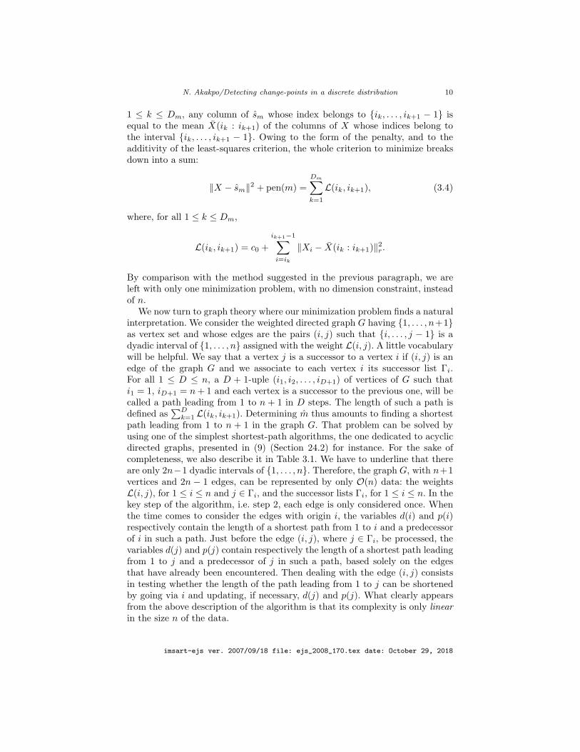
Table 3.1

Algorithm for computing s

Step 1 : InitializationSet d(1) = 0 and p(1) = +∞.For i = 2, . . . , n+ 1,

set d(i) = +∞ and p(i) = +∞.

Step 2 : Determining the lengths of the shortest paths with origin 1For i = 1, . . . , n,

for j ∈ Γi,if d(j) > d(i) + L(i, j),

then do d(j)← d(i) + L(i, j) and p(j)← i.

Step 3 : Determining a shortest path P from 1 to n+ 1Set pred = p(n+ 1) and P = (n+ 1).While pred 6= +∞,

replace P with the concatenation of pred followed by P ,do pred← p(pred).

Step 4 : Computing the preliminary estimatorSet D = length(P )− 1.For k = 1, . . . , D,

for i = P (k), . . . , P (k + 1) − 1,set si = X(P (k) : P (k + 1)).

4. Hybrid estimator

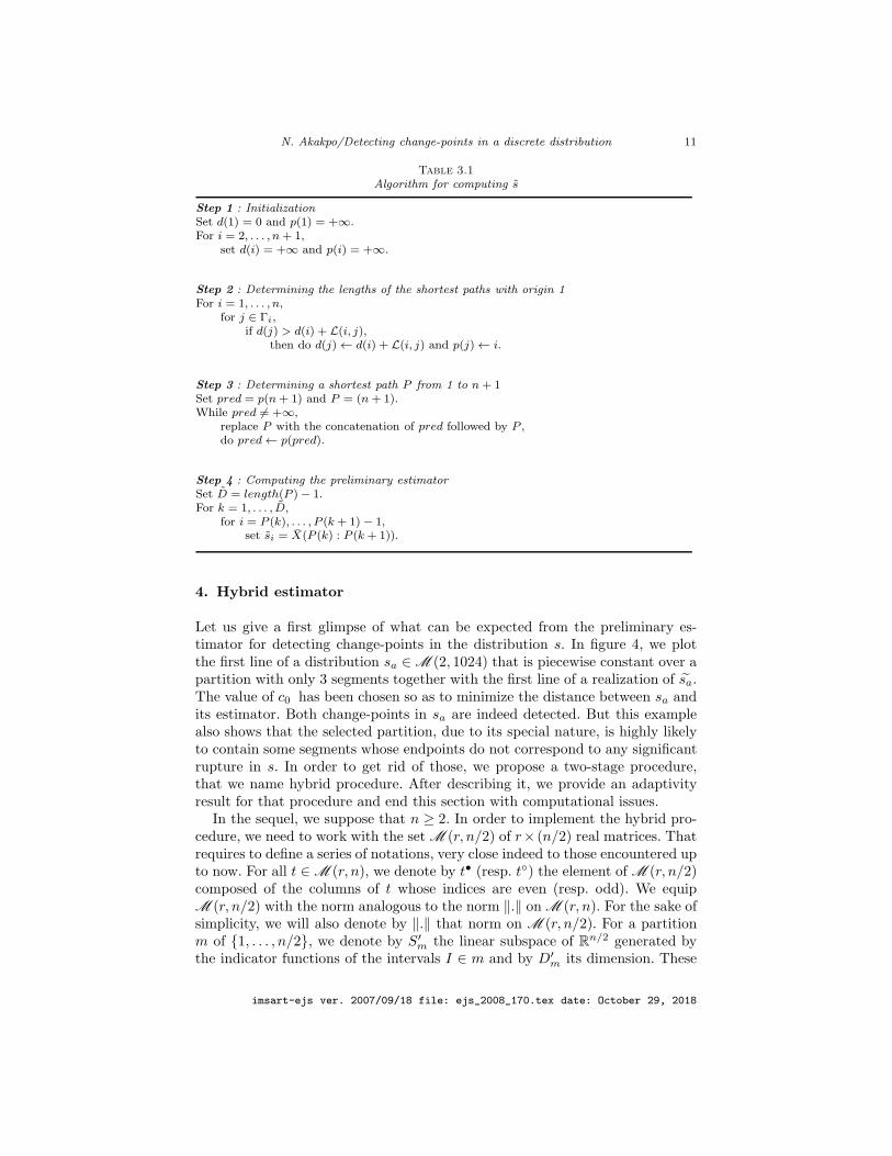
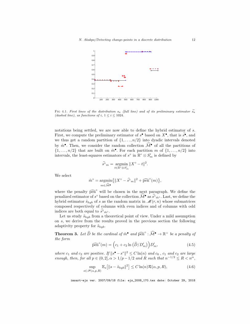
Let us give a first glimpse of what can be expected from the preliminary es-timator for detecting change-points in the distribution s. In figure 4, we plotthe first line of a distribution sa ∈ M (2, 1024) that is piecewise constant over apartition with only 3 segments together with the first line of a realization of sa.The value of c0 has been chosen so as to minimize the distance between sa andits estimator. Both change-points in sa are indeed detected. But this examplealso shows that the selected partition, due to its special nature, is highly likelyto contain some segments whose endpoints do not correspond to any significantrupture in s. In order to get rid of those, we propose a two-stage procedure,that we name hybrid procedure. After describing it, we provide an adaptivityresult for that procedure and end this section with computational issues.

In the sequel, we suppose that n ≥ 2. In order to implement the hybrid pro-cedure, we need to work with the set M (r, n/2) of r× (n/2) real matrices. Thatrequires to define a series of notations, very close indeed to those encountered upto now. For all t ∈ M (r, n), we denote by t• (resp. t) the element of M (r, n/2)composed of the columns of t whose indices are even (resp. odd). We equipM (r, n/2) with the norm analogous to the norm ‖.‖ on M (r, n). For the sake ofsimplicity, we will also denote by ‖.‖ that norm on M (r, n/2). For a partitionm of 1, . . . , n/2, we denote by S′

m the linear subspace of Rn/2 generated bythe indicator functions of the intervals I ∈ m and by D′

m its dimension. These



100 200 300 400 500 600 700 800 900 10000

0.1

0.2

0.3

0.4

0.5

0.6

0.7

0.8

0.9

1

Fig 4.1. First lines of the distribution sa (full line) and of its preliminary estimator sa(dashed line), as functions of i, 1 ≤ i ≤ 1024.

notations being settled, we are now able to define the hybrid estimator of s.First, we compute the preliminary estimator of s• based on X•, that is s•, andwe thus get a random partition of 1, . . . , n/2 into dyadic intervals denoted

by m•. Then, we consider the random collection M• of all the partitions of1, . . . , n/2 that are built on m•. For each partition m of 1, . . . , n/2 intointervals, the least-squares estimators of s in R

r ⊗ S′m is defined by

sm = argmint∈Rr⊗S′

m

‖X − t‖2.

We selectm = argmin

m∈M•

‖X − sm‖2 + pen

(m)

,

where the penalty penwill be chosen in the next paragraph. We define the

penalized estimator of s based on the collection M• as sm . Last, we define thehybrid estimator shyb of s as the random matrix in M (r, n) whose submatricescomposed respectively of columns with even indices and of columns with oddindices are both equal to sm .

Let us study shyb from a theoretical point of view. Under a mild assumptionon s, we derive from the results proved in the previous section the followingadaptivity property for shyb.

Theorem 3. Let D be the cardinal of m• and pen: M• → R

+ be a penalty ofthe form

pen(m) =

(c1 + c2 ln

(D/D′

m

))D′

m, (4.5)

where c1 and c2 are positive. If ‖s•− s‖2 ≤ C ln(n) and c0 , c1 and c2 are largeenough, then, for all p ∈ (0, 2], α > 1/p− 1/2 and R such that n−1/2 ≤ R < nα,

sups∈P(α,p,R)

Es

[‖s− shyb‖2

]≤ C ln(n)R(α, p,R), (4.6)



where C only depends on c0, c1, c2, α and p.

Thus, with Inequality (4.6), we recover a result similar to Inequality (3.3), upto a logarithmic factor.

Proof. For all 1 ≤ D ≤ D, the number ND of partitions in M• with D piecessatisfies

ND =

(D − 1

D − 1

)≤(eD

D

)D

.

The above inequality results from a property of binomial coefficients that maybe found in (18) (Proposition 2.5) for instance. So the weights defined by

L(D) = ln(2e) + ln(D/D), for 1 ≤ D ≤ D,

are such thatD∑

D=1

ND exp(−DL(D)) ≤ 1.

Moreover, the penalty pengiven by (4.5) fulfills the hypotheses of Theorem 1

in (13) provided c1 and c2 are large enough. With a slight abuse of notation, forany partition m of 1, . . . , n/2, we still denote by tm the orthogonal projectionof an element t ∈ M (r, n/2) on R

r ⊗ S′m. Working conditionally to X•, the

collection M• is deterministic, so we deduce from Theorem 1 of (13) applied tothe estimator sm of s that

Es[‖s − sm‖2|X•

]≤ C(c1, c2)

[‖s − sm•‖2 + pen(m•)

]. (4.7)

We recall that s• = s•m• . So, thanks to the triangle inequality, and since anorthogonal projection is a shrinking map, we get

‖s − sm•‖2 ≤ C(‖s − s•‖2 + ‖s• − s•‖2

).

Besides, for all m ∈ M•,

pen(m) ≤ C(c1, c2) ln(n)D′m.

Taking into account the last two inequalities and integrating with respect to X•

then leads from (4.7) to

Es

[‖s − sm‖2

]≤ C(c1, c2)

[‖s − s•‖2 + Es•

[‖s• − s•‖2

]+ ln(n)Es•(D

′m•)],

where D′m• is nothing but D. Besides, it follows from the definition of shyb that

‖s− shyb‖2 = ‖s• − sm‖2 + ‖s − sm‖2.

Applying the triangle inequality, we then get

‖s− shyb‖2 ≤ C(‖s• − s‖2 + ‖s − sm‖2

).



Consequently,

Es

[‖s− shyb‖2

]≤ C(c1, c2)

[‖s−s•‖2+Es•

[‖s•− s•‖2

]+ln(n)Es•(D)

]. (4.8)

Let us denote byM′ the set of all partitions of 1, . . . , n/2 into dyadic intervals.For the risk of s•, Theorem 1 of (13) provides

Es•[‖s• − s•‖2

]≤ C(c0) inf

m∈M′

‖s• − s•m‖2 +D′

m

. (4.9)

In order to bound the term Es•(D), we need to go back to the proof of Theorem1 in (13) (Section 8.1). As already seen during the proof of Proposition 1, wecan choose a positive constant L such that

∑m∈M′ exp(−LD′

m) ≤ 1. Let us fixa partition m ∈ M′ and ξ > 0. Using the same notation as in (13), we deducefrom the proof of Theorem 1 in (13) that there exists an event Ωξ(m) such thatPs•(Ωξ(m)) ≥ 1− exp(−ξ) and on which

c0D ≤ C1‖s• − s•m‖2 + C2(c0)D′m + C3D + C4ξ.

Therefore, if c0 > C3, then

D ≤ C(c0)(‖s• − s•m‖2 +D′

m + ξ).

Integrating this inequality and taking the infimum over m ∈ M′ then yields

Es•(D) ≤ C(c0) infm∈M′

‖s• − s•m‖2 +D′

m

. (4.10)

Moreover, one can check that

infm∈M′

‖s• − s•m‖2 +D′

m

≤ inf

m∈M

‖s− sm‖2 +Dm

. (4.11)

Combining Inequalities (4.8) to (4.11) and the assumption on ‖s• − s‖2, wefinally get

Es

[‖s− shyb‖2

]≤ C(c0, c1, c2) ln(n) inf

m∈M

‖s− sm‖2 +Dm

.

We then conclude the proof as that of Theorem 2.

Regarding the computation of shyb, we know from Section 3.3 that deter-mining s• only requires O(n) computations. On the other hand, since pen isnot linear in the dimension of the models, m has to be determined followingthe method suggested at the beginning of Section 3.3 and using Bellman’s al-gorithm. If we impose an upper-bound Dmax on the dimension of the modelselected during the second stage, determining m given X• then requires of theorder of D2Dmax computations. Since D is upper-bounded by n/2, we can onlyensure that the computational complexity of shyb is, in the worst case, of theorder of n2Dmax. However, we will see in Section 5 that, in practice, the hybridprocedure can also be implemented with a linear complexity only and with quitesatisfactory results.



5. Simulation study

In the previous sections, we were only interested in giving a form of penaltyyielding, in theory, a performant estimator. The aim of this section is to studypractical choices of the penalty for each procedure. Several simulations allowto assess the relevance of these choices and to illustrate the qualities of eachprocedure.

5.1. Choosing the penalty constant for the preliminary estimator

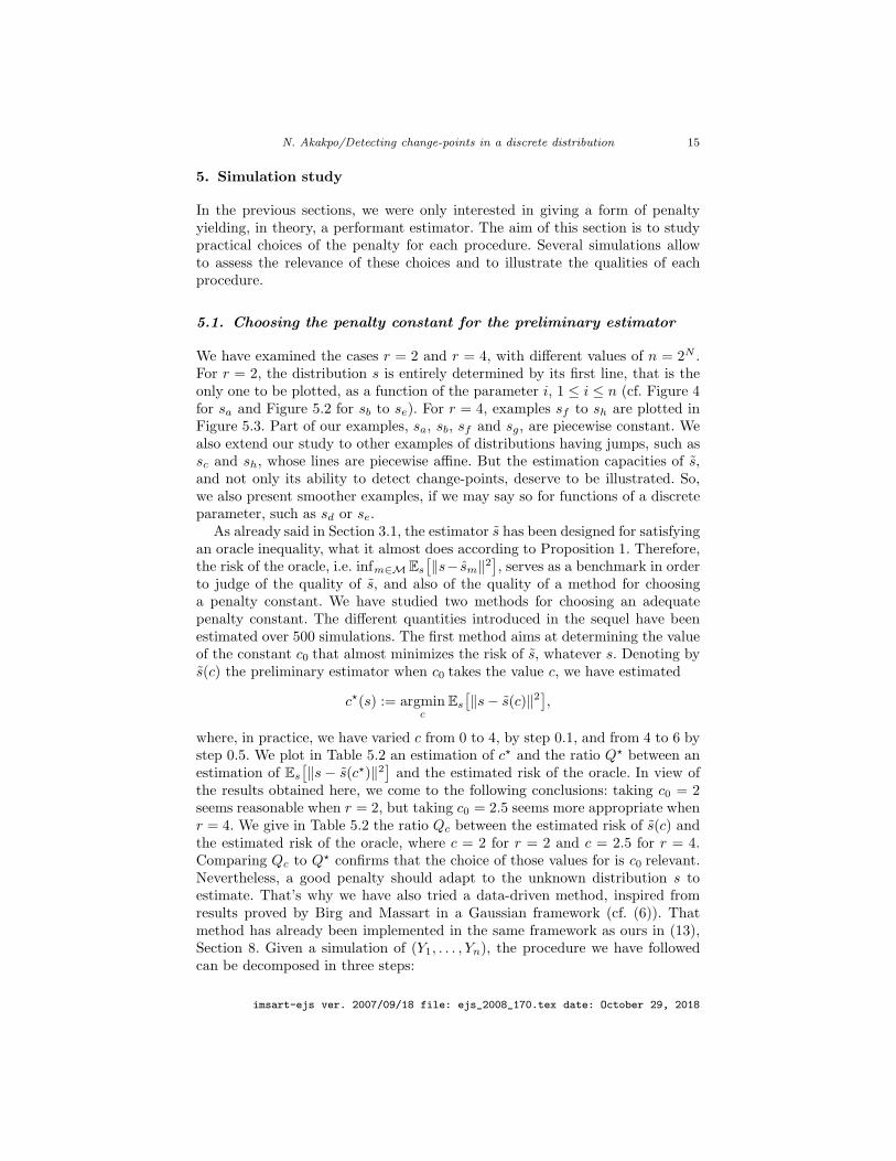
We have examined the cases r = 2 and r = 4, with different values of n = 2N .For r = 2, the distribution s is entirely determined by its first line, that is theonly one to be plotted, as a function of the parameter i, 1 ≤ i ≤ n (cf. Figure 4for sa and Figure 5.2 for sb to se). For r = 4, examples sf to sh are plotted inFigure 5.3. Part of our examples, sa, sb, sf and sg, are piecewise constant. Wealso extend our study to other examples of distributions having jumps, such assc and sh, whose lines are piecewise affine. But the estimation capacities of s,and not only its ability to detect change-points, deserve to be illustrated. So,we also present smoother examples, if we may say so for functions of a discreteparameter, such as sd or se.

As already said in Section 3.1, the estimator s has been designed for satisfyingan oracle inequality, what it almost does according to Proposition 1. Therefore,the risk of the oracle, i.e. infm∈M Es

[‖s− sm‖2

], serves as a benchmark in order

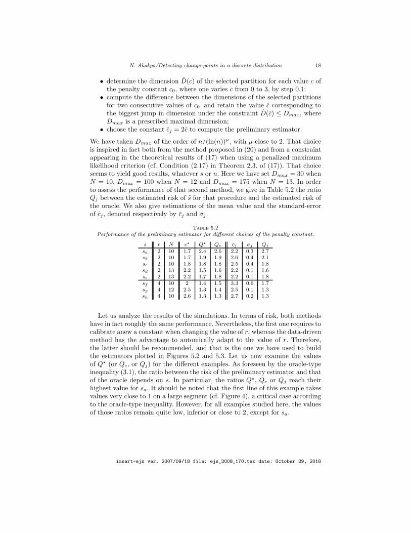
to judge of the quality of s, and also of the quality of a method for choosinga penalty constant. We have studied two methods for choosing an adequatepenalty constant. The different quantities introduced in the sequel have beenestimated over 500 simulations. The first method aims at determining the valueof the constant c0 that almost minimizes the risk of s, whatever s. Denoting bys(c) the preliminary estimator when c0 takes the value c, we have estimated

c⋆(s) := argminc

Es

[‖s− s(c)‖2

],

where, in practice, we have varied c from 0 to 4, by step 0.1, and from 4 to 6 bystep 0.5. We plot in Table 5.2 an estimation of c⋆ and the ratio Q⋆ between anestimation of Es

[‖s− s(c⋆)‖2

]and the estimated risk of the oracle. In view of

the results obtained here, we come to the following conclusions: taking c0 = 2seems reasonable when r = 2, but taking c0 = 2.5 seems more appropriate whenr = 4. We give in Table 5.2 the ratio Qc between the estimated risk of s(c) andthe estimated risk of the oracle, where c = 2 for r = 2 and c = 2.5 for r = 4.Comparing Qc to Q⋆ confirms that the choice of those values for is c0 relevant.Nevertheless, a good penalty should adapt to the unknown distribution s toestimate. That’s why we have also tried a data-driven method, inspired fromresults proved by Birg and Massart in a Gaussian framework (cf. (6)). Thatmethod has already been implemented in the same framework as ours in (13),Section 8. Given a simulation of (Y1, . . . , Yn), the procedure we have followedcan be decomposed in three steps:



100 200 300 400 500 600 700 800 900 10000

0.2

0.4

0.6

0.8

1b

100 200 300 400 500 600 700 800 900 10000

0.2

0.4

0.6

0.8

1c

1000 2000 3000 4000 5000 6000 7000 80000

0.2

0.4

0.6

0.8

1e

1000 2000 3000 4000 5000 6000 7000 80000

0.2

0.4

0.6

0.8

1d

Fig 5.2. First lines of s (full line) and s (dashed line), computed with a data-drivenpenalty, for s ∈ sb, sc, sd, se.



100 200 300 400 500 600 700 800 900 10000

0.5

1

100 200 300 400 500 600 700 800 900 10000

0.5

1

100 200 300 400 500 600 700 800 900 10000

0.5

1

100 200 300 400 500 600 700 800 900 10000

0.5

1f

500 1000 1500 2000 2500 3000 3500 40000

0.5

1

500 1000 1500 2000 2500 3000 3500 40000

0.5

1

500 1000 1500 2000 2500 3000 3500 40000

0.5

1

500 1000 1500 2000 2500 3000 3500 40000

0.5

1g

100 200 300 400 500 600 700 800 900 10000

0.5

1h

100 200 300 400 500 600 700 800 900 10000

0.5

1

100 200 300 400 500 600 700 800 900 10000

0.5

1

100 200 300 400 500 600 700 800 900 10000

0.5

1

Fig 5.3. Four lines of s (full line) and s (dashed line), computed with a data-drivenpenalty, for s ∈ sf , sg, sh.



• determine the dimension D(c) of the selected partition for each value c ofthe penalty constant c0, where one varies c from 0 to 3, by step 0.1;

• compute the difference between the dimensions of the selected partitionsfor two consecutive values of c0 and retain the value c corresponding tothe biggest jump in dimension under the constraint D(c) ≤ Dmax, whereDmax is a prescribed maximal dimension;

• choose the constant cj = 2c to compute the preliminary estimator.

We have taken Dmax of the order of n/(ln(n))µ, with µ close to 2. That choiceis inspired in fact both from the method proposed in (20) and from a constraintappearing in the theoretical results of (17) when using a penalized maximumlikelihood criterion (cf. Condition (2.17) in Theorem 2.3. of (17)). That choiceseems to yield good results, whatever s or n. Here we have set Dmax = 30 whenN = 10, Dmax = 100 when N = 12 and Dmax = 175 when N = 13. In orderto assess the performance of that second method, we give in Table 5.2 the ratioQj between the estimated risk of s for that procedure and the estimated risk ofthe oracle. We also give estimations of the mean value and the standard-errorof cj , denoted respectively by cj and σj .

Table 5.2

Performance of the preliminary estimator for different choices of the penalty constant.

s r N c⋆ Q⋆ Qc cj σj Qj

sa 2 10 1.7 2.4 2.6 2.2 0.3 2.7sb 2 10 1.7 1.9 1.9 2.6 0.4 2.1sc 2 10 1.8 1.8 1.8 2.5 0.4 1.8sd 2 13 2.2 1.5 1.6 2.2 0.1 1.6se 2 13 2.2 1.7 1.8 2.2 0.1 1.8sf 4 10 2 1.4 1.5 3.3 0.6 1.7sg 4 12 2.5 1.3 1.4 2.5 0.1 1.3sh 4 10 2.6 1.3 1.3 2.7 0.2 1.3

Let us analyze the results of the simulations. In terms of risk, both methodshave in fact roughly the same performance. Nevertheless, the first one requires tocalibrate anew a constant when changing the value of r, whereas the data-drivenmethod has the advantage to automically adapt to the value of r. Therefore,the latter should be recommended, and that is the one we have used to buildthe estimators plotted in Figures 5.2 and 5.3. Let us now examine the valuesof Q⋆ (or Qc, or Qj) for the different examples. As foreseen by the oracle-typeinequality (3.1), the ratio between the risk of the preliminary estimator and thatof the oracle depends on s. In particular, the ratios Q⋆, Qc or Qj reach theirhighest value for sa. It should be noted that the first line of this example takesvalues very close to 1 on a large segment (cf. Figure 4), a critical case accordingto the oracle-type inequality. However, for all examples studied here, the valuesof those ratios remain quite low, inferior or close to 2, except for sa.



5.2. Choosing the penalty constants for the hybrid estimator

For the first stage of the hybrid procedure, the preliminary estimator has beencomputed using the data-driven penalty. For the second stage, the practicalchoice of an adequate penalty is more delicate, since the theoretical penaltydepends in this case on two constants and on the dimension D of the partitionselected during the first stage. We have first tried here the same method asLebarbier in (16), Chapter 7, for her own hybrid procedure. So we have assignedto all partitions of 1, . . . , n/2 into D intervals the same penalty

pen1(D) = β1(2.5 + ln(D/D))D,

where β1 is determined according to the same process as cj . That penalty is pro-portional to the penalty calibrated by Lebarbier in (16) (Chapter 3). The latterwas in fact designed for the estimation of a regression function in a Gaussianframework via model selection based on an exhaustive collection of partitions.Anyway, the major drawback of such a method, as said at the end of Section 4, isthat we are only able to evaluate its worst case computational complexity, of theorder of O(n3). So we have also tried to assign to all partitions of 1, . . . , n/2into D intervals the penalty

pen2(D) = β2D,

where β2 is determined once again according to the same process as cj . Sincethat penalty is a linear funtion of D, the hybrid procedure can be implementedin that case with only O(n) computations.

In order to draw a comparison between these procedures and with the pre-liminary one, we give in Table 5.3 the following information for the distributionssa to sc and sf to sg, still computed over 500 simulations. We first recall thedimension D of the partition on which s is built. Then we indicate the averagedimensions D0 and Di of the partitions selected respectively by the preliminaryprocedure, with a data-driven penalty, and the hybrid procedure with pen

i , for

i ∈ 1, 2. We also give the average value Qi:0 of the ratio between the estimatedrisk of the hybrid estimator for pen

i , for i ∈ 1, 2, and the estimated risk ofthe preliminary estimator. Let us compare both ways to implement the hybridprocedure. We observe that Q2:0 is almost always of the same order as Q1:0, andeven slightly lower in most cases. Therefore, taking into account the computa-tional complexity, we cannot but recommend to use pen

2. That is the choice we

have made for the hybrid estimators represented in Figures 5.4 and 5.5. Let usnow compare the hybrid procedure with the preliminary one for the examplesunder study. First, the values of D2 and D0 indicate that, with the former, thedimension of the selected partition is much closer to the true one. Moreover, thefigures show that the most significant ruptures are still detected, are quite closeto the true ones, and that irrelevant ruptures are much fewer with the hybridprocedure. The only price to pay is an increase in risk, but only by a factor ofthe order of 1.5.



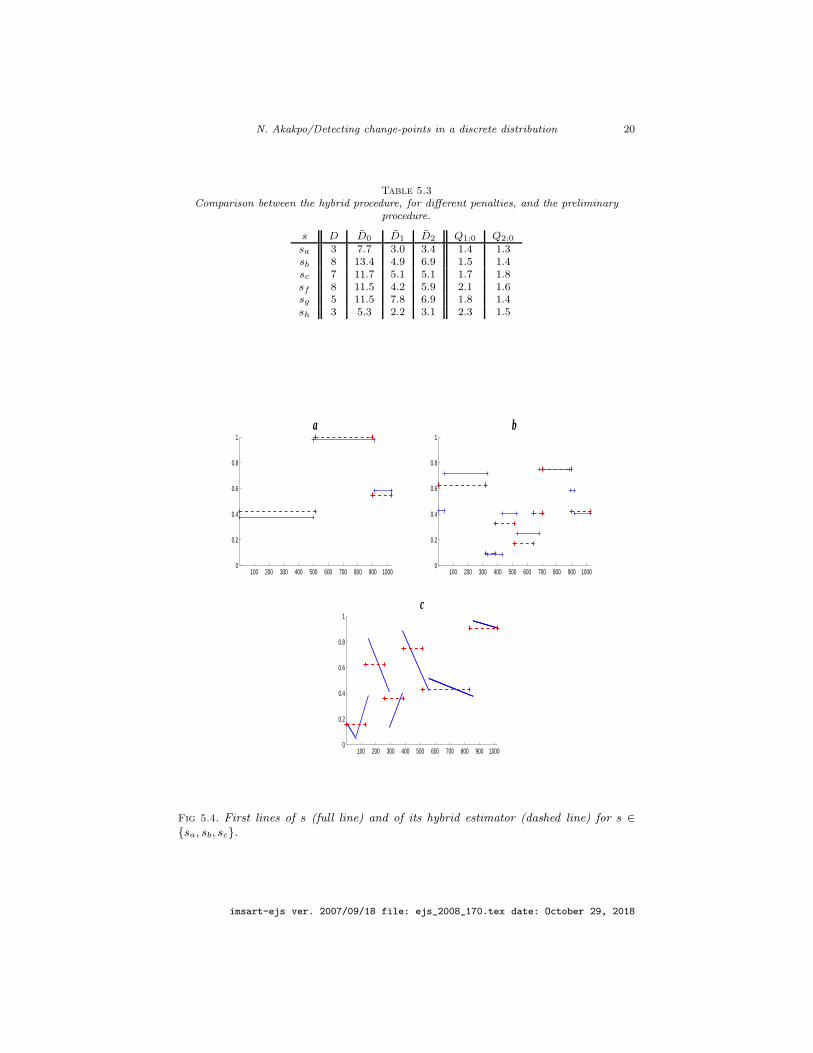
Table 5.3

Comparison between the hybrid procedure, for different penalties, and the preliminaryprocedure.

s D D0 D1 D2 Q1:0 Q2:0

sa 3 7.7 3.0 3.4 1.4 1.3sb 8 13.4 4.9 6.9 1.5 1.4sc 7 11.7 5.1 5.1 1.7 1.8sf 8 11.5 4.2 5.9 2.1 1.6sg 5 11.5 7.8 6.9 1.8 1.4sh 3 5.3 2.2 3.1 2.3 1.5

100 200 300 400 500 600 700 800 900 10000

0.2

0.4

0.6

0.8

1a

100 200 300 400 500 600 700 800 900 10000

0.2

0.4

0.6

0.8

1b

100 200 300 400 500 600 700 800 900 10000

0.2

0.4

0.6

0.8

1c

Fig 5.4. First lines of s (full line) and of its hybrid estimator (dashed line) for s ∈sa, sb, sc.



100 200 300 400 500 600 700 800 900 10000

0.5

1

100 200 300 400 500 600 700 800 900 10000

0.5

1

100 200 300 400 500 600 700 800 900 10000

0.5

1

100 200 300 400 500 600 700 800 900 10000

0.5

1f

500 1000 1500 2000 2500 3000 3500 40000

0.5

1g

500 1000 1500 2000 2500 3000 3500 40000

0.5

1

500 1000 1500 2000 2500 3000 3500 40000

0.5

1

500 1000 1500 2000 2500 3000 3500 40000

0.5

1

100 200 300 400 500 600 700 800 900 10000

0.5

1h

100 200 300 400 500 600 700 800 900 10000

0.5

1

100 200 300 400 500 600 700 800 900 10000

0.5

1

100 200 300 400 500 600 700 800 900 10000

0.5

1

Fig 5.5. Four lines of sf , sg and sh (full line) together with their hybrid estimators(dashed line).



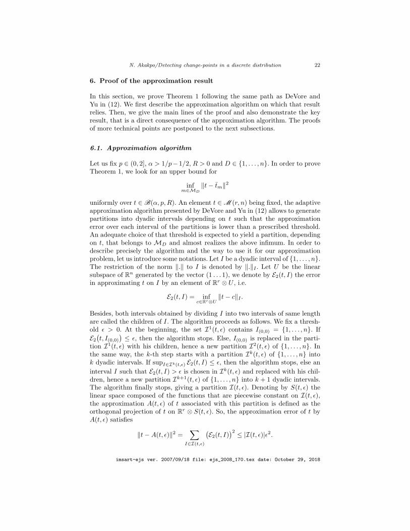
6. Proof of the approximation result

In this section, we prove Theorem 1 following the same path as DeVore andYu in (12). We first describe the approximation algorithm on which that resultrelies. Then, we give the main lines of the proof and also demonstrate the keyresult, that is a direct consequence of the approximation algorithm. The proofsof more technical points are postponed to the next subsections.

6.1. Approximation algorithm

Let us fix p ∈ (0, 2], α > 1/p− 1/2, R > 0 and D ∈ 1, . . . , n. In order to proveTheorem 1, we look for an upper bound for

infm∈MD

‖t− tm‖2

uniformly over t ∈ B(α, p,R). An element t ∈ M (r, n) being fixed, the adaptiveapproximation algorithm presented by DeVore and Yu in (12) allows to generatepartitions into dyadic intervals depending on t such that the approximationerror over each interval of the partitions is lower than a prescribed threshold.An adequate choice of that threshold is expected to yield a partition, dependingon t, that belongs to MD and almost realizes the above infimum. In order todescribe precisely the algorithm and the way to use it for our approximationproblem, let us introduce some notations. Let I be a dyadic interval of 1, . . . , n.The restriction of the norm ‖.‖ to I is denoted by ‖.‖I . Let U be the linearsubspace of Rn generated by the vector (1 . . . 1), we denote by E2(t, I) the errorin approximating t on I by an element of Rr ⊗ U , i.e.

E2(t, I) = infc∈Rr⊗U

‖t− c‖I .

Besides, both intervals obtained by dividing I into two intervals of same lengthare called the children of I. The algorithm proceeds as follows. We fix a thresh-old ǫ > 0. At the beginning, the set I1(t, ǫ) contains I(0,0) = 1, . . . , n. IfE2(t, I(0,0)

)≤ ǫ, then the algorithm stops. Else, I(0,0) is replaced in the parti-

tion I1(t, ǫ) with his children, hence a new partition I2(t, ǫ) of 1, . . . , n. Inthe same way, the k-th step starts with a partition Ik(t, ǫ) of 1, . . . , n intok dyadic intervals. If supI∈Ik(t,ǫ) E2(t, I) ≤ ǫ, then the algorithm stops, else an

interval I such that E2(t, I) > ǫ is chosen in Ik(t, ǫ) and replaced with his chil-dren, hence a new partition Ik+1(t, ǫ) of 1, . . . , n into k + 1 dyadic intervals.The algorithm finally stops, giving a partition I(t, ǫ). Denoting by S(t, ǫ) thelinear space composed of the functions that are piecewise constant on I(t, ǫ),the approximation A(t, ǫ) of t associated with this partition is defined as theorthogonal projection of t on R

r ⊗ S(t, ǫ). So, the approximation error of t byA(t, ǫ) satisfies

‖t−A(t, ǫ)‖2 =∑

I∈I(t,ǫ)

(E2(t, I)

)2 ≤ |I(t, ǫ)|ǫ2.



For any ǫ > 0 such that the algorithm stops at the latest at step D, the approx-imation of t that we get belongs to the collection Rr ⊗ Smm∈MD

. Therefore

infm∈MD

‖t− tm‖2 ≤ |I(t, ǫ)|ǫ2.

Let us denote by ED(t) the infimum of |I(t, ǫ)|ǫ2 taken over all ǫ > 0 satisfying|I(t, ǫ)| ≤ D. This is in fact the quantity that we shall bound, as indicated inTheorem 4 below.

Theorem 4. Let p ∈ (0, 2], α > 1/p− 1/2 and R > 0. For all D ∈ 1, . . . , nand t ∈ B(α, p,R),

ED(t) ≤ C(α, p)nR2D−2α.

We then get Theorem 1 as a straightforward consequence of Theorem 4.

6.2. Proof of Theorem 4: the main lines

Here are the notions and notations that we will need along the proof. Let p > 0,α > 0 and t ∈ M (r, n). For every subset I of 1, . . . , n, let

Ep(t, I) = infv∈Rr

(∑

k∈I

‖tk − v‖pr)1/p

.

We define the vector t♯,α,p in Rn whose coordinates are

t♯,α,pi = supI∋i

|I|−(α+1/p)Ep(t, I), for i = 1, . . . , n,

where the supremum is taken over all the dyadic intervals I of 1, . . . , n thatcontain i. We denote by ‖.‖ℓp the (quasi-)norm defined on R

n by

‖u‖ℓp =

( n∑

i=1

|ui|p)1/p

(that is a norm only for p ≥ 1) and by ‖.‖ℓp,I its restriction to a subset I of1, . . . , n. We define on R

n the discrete Hardy-Littlewood maximal functionMp by (

Mp(u))i= sup

I∋i|I|−1/p‖u‖ℓp,I , for i = 1, . . . , n,

where the supremum is taken over all the dyadic intervals I of 1, . . . , n con-taining i. Last, we recall that every vector u ∈ R

n is identified with the functiondefined on 1, . . . , n whose value in i is ui, for 1 ≤ i ≤ n, hence the meaningof notations such as u ≤ v or uq, where u ∈ R

n, v ∈ Rn and q > 0.

The beginning of the proof directly results from the way the algorithm worksout. A dimension D being fixed, choosing ǫ > 0 as small as possible such thatthe algorithm generates a partition with at most D intervals leads to a firstcomparison between the quantity ED(t) and D−2α, without making use of anyparticular hypothesis on t.



Proposition 2. Let α > 0 and p(α) = (α+1/2)−1. For all D ∈ 1, . . . , n andt ∈ M (r, n),

ED(t) ≤ C(α)‖t♯,α,2‖2ℓp(α)D−2α.

Proof. If t♯,α,2 = 0, then, whatever ǫ > 0, E2(t, I(0,0)

)≤ ǫ, so ED(t) = 0, which

completes the proof in that case. Let us now suppose that t♯,α,2 is non-null, andlet ǫ > 0. If E2

(t, I(0,0)

)≤ ǫ, then |I(t, ǫ)| = 1. Else, let I be a dyadic interval

that belongs to I(t, ǫ), then I is a child of a dyadic interval I such that

ǫ < E2(t, I).

Using the definition of t♯,α,2, we get, for all i ∈ I,

E2(t, I)≤∣∣I∣∣α+1/2

t♯,α,2i .

Since I ⊂ I, |I| = 2|I| and p(α) = (α + 1/2)−1, the last two inequalities lead,for all i ∈ I, to

ǫ < 21/p(α)|I|1/p(α)t♯,α,2i ,

hence

ǫp(α) < 2∑

i∈I

(t♯,α,2i

)p(α).

Then we deduce by summing over all the intervals I in the partition I(t, ǫ) that

|I(t, ǫ)| ≤ 2‖t♯,α,2‖p(α)ℓp(α)ǫ−p(α).

Whether E2(t, I(0,0)

)≤ ǫ or not, by choosing ǫ = 21/p(α)‖t♯,α,2‖ℓp(α)

D−1/p(α),

we get a partition I(t, ǫ) that contains at most D elements and satisfies

|I(t, ǫ)|ǫ2 ≤ D1−2/p(α)22/p(α)‖t♯,α,2‖2ℓp(α).

As p(α) = (α+ 1/2)−1, we conclude that

|I(t, ǫ)|ǫ2 ≤ 4α+1/2‖t♯,α,2‖2ℓp(α)D−2α.

The proof of Theorem 4 now relies upon three inequalities. The first oneallows to draw a comparison between ED(t) and D−2α via a term that doesnot depend on t♯,α,2 anymore but on t♯,α,p(α). It is the discrete analogue of aparticular case of Theorem 4.3. of (11).

Proposition 3. Let α > 0 and p(α) = (α+ 1/2)−1. For all t ∈ M (r, n),

t♯,α,2 ≤ C(α)Mp(α)

(t♯,α,p(α)

).



From Propositions 2 and 3, we easily deduce that, for α > 0, p(α) = (α+1/2)−1

and D ∈ 1, . . . , n,

ED(t) ≤ C(α)∥∥Mp(α)

(t♯,α,p(α)

)∥∥2ℓp(α)

D−2α.

Let us now fix p ∈ (0, 2]. By Jensen’s inequality, we have

∥∥Mp(α)

(t♯,α,p(α)

)∥∥ℓp(α)

≤ n1/p(α)−1/p∥∥Mp(α)

(t♯,α,p(α)

)∥∥ℓp

andt♯,α,p(α) ≤ t♯,α,p,

henceED(t) ≤ C(α)n2(α+1/2−1/p)

∥∥Mp(α)(t♯,α,p)

∥∥2ℓpD−2α.

Though the most obvious comparison between a vector u and any of its maxi-mal functions is that the latter are greater than the first, the following maximalinequality also ensures a control of u over its maximal functions (cf. inequal-ity (6.12) below). That inequality is in fact the discrete version of a fundamentalresult in functional analysis, namely the Hardy-Littlewood maximal inequality,that may be found in (2) (Theorem 3.10) for instance.

Proposition 4. Let q > 1. For all u ∈ Rn,

‖M1(u)‖ℓq ≤ C(q)‖u‖ℓq .

Since the maximal function Mq, q > 0, is related to M1 by the property

Mq(u) =(M1(u

q))1/q

, for all u ∈ Rn,

Proposition 4 yields, for all r > q > 0 and u ∈ Rn,

‖Mq(u)‖ℓr ≤ C(r, q)‖u‖ℓr . (6.12)

Thus, when applied with u = t♯,α,p, r = p and q = p(α), this inequality leads to

ED(t) ≤ C(α, p)n2(α+1/2−1/p)‖t♯,α,p‖2ℓpD−2α.

Last, Proposition 5 below provides the adequate control of the ℓp-(quasi-)normof t♯,α,p by the size of the wavelet coefficients of t and allows to complete imme-diately the proof of Theorem 4.

Proposition 5. Let p ∈ (0, 2] and α > 1/p− 1/2. For all t ∈ M (r, n),

‖t♯,α,p‖ℓp ≤ C(α, p)n−(α+1/2−1/p)

(N−1∑

j=0

2jp(α+1/2−1/p)∑

λ∈Λ(j)

‖βλ‖pr

)1/p

,

where, for all λ ∈ Λ, βλ stands for the column vector of Rr whose l-th line is

β(l)λ = 〈t(l), φλ〉n, for l = 1, . . . , r.



6.3. Proofs of Propositions 3 and 4

We present in a same section the proofs of Propositions 3 and 4, that bothmainly call for the notion of decreasing rearrangement of a vector in R

n.

Definition 3. Let u ∈ Rn. The decreasing rearrangement of u is the R

n- vectordenoted by u⋆ satisfying

u⋆1 ≥ u⋆2 ≥ . . . ≥ u⋆n and u⋆i ; 1 ≤ i ≤ n = |ui|; 1 ≤ i ≤ n.

We will also make use of the Lorentz (quasi-)norms on Rn in the proof of Propo-

sition 3, whose definition we recall here.

Definition 4. Let 0 < p < +∞ and 0 < q ≤ +∞. We denote by ‖.‖ℓp,q theLorentz (quasi-)norm defined on R

n by:

• if q is finite, ‖u‖ℓp,q =(∑n

i=1 i−1(i1/pu⋆i )

q)1/q

;

• if q = +∞, ‖u‖ℓp,∞ = sup1≤i≤n i1/pu⋆i .

For all subset I of 1, . . . , n, we denote by ‖.‖ℓp,q,I the restriction of ‖.‖ℓp,q toI. In particular, notice that, for all u ∈ R

n, 0 < p < +∞ and 0 < q ≤ +∞,

‖u‖ℓp,p = ‖u‖ℓp and ‖u⋆‖ℓp,q = ‖u‖ℓp,q .

The reader may find in the appendix other useful properties relative to thesenotions.

6.3.1. Proof of Proposition 3

The proof of Proposition 3 mostly relies on a lemma that we demonstrate inthis paragraph, after introducing a few notations. Let I be a dyadic interval of1, . . . , n, t ∈ M (r, n), and p > 0. By a compactness argument, there existsat least one vector in R

r, denoted by vp(t, I), realizing the error Ep(t, I), i.e.satisfying

Ep(t, I) =(∑

k∈I

‖tk − vp(t, I)‖pr)1/p

.

We define the vectors up(t, I) and t♯,α,p,I in Rn whose coordinates are null

outside of I and given otherwise respectively by

(up(t, I)

)i= ‖ti − vp(t, I)‖r, for i ∈ I,

andt♯,α,p,Ii = sup

I⊃J∋i|J |−(α+1/p)Ep(t, J), for i ∈ I,

where the supremum is taken over all the dyadic intervals J of 1, . . . , n thatare contained in I and contain i.



Lemma 1. Let α > 0, p > 0 and t ∈ M (r, n). Let I be a dyadic interval of1, . . . , n containing at least two elements. For all j ∈ 1, . . . , |I|/2,

(up(t, I)

)⋆j≤ C(α, p)

(|I|/2∑

k=j

kα−1(t♯,α,p,I

)⋆k+ jα

(t♯,α,p,I

)⋆j

).

Proof. We fix j ∈ 1, . . . , |I|/2. Let E be the set composed of all the indices iin 1, . . . , n satisfying (t♯,α,p,I)i > (t♯,α,p,I)⋆j . As |E| ≤ j − 1, we only have toprove that

(up(t, I)

)i≤ C(α, p)

(|I|/2∑

k=j

kα−1(t♯,α,p,I

)⋆k+ jα

(t♯,α,p,I

)⋆j

)(6.13)

for all the indices i ∈ 1, . . . , n, except maybe for those belonging to E. Con-sider i ∈ 1, . . . , n such that i /∈ E. If i /∈ I, then

(up(t, I)

)i= 0, so Inequal-

ity (6.13) is trivial. Suppose now that i ∈ I and i /∈ E, and let Il1≤l≤m be thesequence of dyadic intervals defined by

I1 = I, Il+1 is the child of Il containing i, and Im = i,

where m ≥ 2 because |I| ≥ 2. Notice that, for all l ∈ 0, . . . ,m − 1, |Il+1| =2−l|I|. Let q be the strictly positive integer such that

2−(q+1)|I| < j ≤ 2−q|I|.

Such a definition implies, in particular, that 2−q|I| ≥ 1, so that q < m. Fromthe triangular inequality,

(up(t, I)

)i≤

q∑

l=2

‖vp(t, Il−1)−vp(t, Il)‖r+m∑

l=q+1

‖vp(t, Il−1)−vp(t, Il)‖r, (6.14)

with the convention that the first sum in Inequality (6.14) is null for q = 1. Letus fix l ∈ 2, . . . ,m and determine an upper-bound for the term ‖vp(t, Il−1)−vp(t, Il)‖r. We recall that Il ⊂ Il−1 and |Il−1| = 2|Il|. Besides, for all p > 0,the (quasi-)norm ‖.‖ℓp satisfies a triangular inequality within a multiplicative

constant C(p), where we can take C(p) = 1 for p ≥ 1, and C(p) = 21/p for0 < p < 1. Therefore, we get

‖vp(t, Il−1)− vp(t, Il)‖r ≤ C(p)|Il|−1/p(Ep(t, Il−1) + Ep(t, Il)

),

which leads to

‖vp(t, Il−1)− vp(t, Il)‖r ≤ C(α, p)|Il|α mink∈Il

t♯,α,p,Ik . (6.15)

Let us bound the first sum appearing in (6.14). For all l ∈ 2, . . . ,m, we have

mink∈Il

t♯,α,p,Ik ≤(t♯,α,p,I

)⋆|Il|

= min1≤k≤|Il|

(t♯,α,p,I

)⋆k,



and, as |Il+1| = |Il|/2,

|Il|α = C(α)

∫ |Il|

|Il+1|

xα−1 dx ≤ C(α)

|Il|∑

k=|Il+1|

kα−1.

Consequently, when q ≥ 2, Inequality (6.15) yields

q∑

l=2

‖vp(t, Il−1)− vp(t, Il)‖r ≤ C(α, p)

q∑

l=2

|Il|∑

k=|Il+1|

kα−1(t♯,α,p,I

)⋆k

≤ C(α, p)

|I|/2∑

k=j

kα−1(t♯,α,p,I

)⋆k.

Regarding the second sum appearing in (6.14), we now use Inequality (6.15)combined with the following remarks. For all l such that q+1 ≤ l ≤ m, we havemink∈Il t

♯,α,p,Ik ≤ t♯,α,p,Ii , since Il contains i, and we recall that |Il| = 2−(l−1)|I|.

Therefore,

m∑

l=q+1

‖vp(t, Il−1)− vp(t, Il)‖r ≤ C(α, p)|I|α(t♯,α,p,I

)i

m∑

l=q+1

2−(l−1)α.

Furthermore, remember that 2−(q+1)|I| < j and i /∈ E, so we finally obtain

m∑

l=q+1

‖vp(t, Il−1)− vp(t, Il)‖r ≤ C(α, p)jα(t♯,α,p,I

)⋆j.

We have thus proved inequality (6.13) and Lemma 1.

We are now able to prove Proposition 3. Let α > 0, p(α) = (α + 1/2)−1 andt ∈ M (r, n). We fix i ∈ 1, . . . , n. From the definition of E2(t, I) for any subsetI of 1, . . . , n, and due to the fact that E2(t, i) = 0, we have

t♯,α,2i ≤ supI∋i

|I|−1/p(α)‖up(α)(t, I)‖ℓ2 ,

where the supremum is taken over all the dyadic intervals I of 1, . . . , n thatcontain i, except for i. We fix such an interval I. The sequence

(up(α)(t, I)

)⋆j

1≤j≤n

decreases and is null for j ≥ |I|+ 1, hence

∥∥up(α)(t, I)∥∥2ℓ2

≤ 2

|I|/2∑

j=1

((up(α)(t, I)

)⋆j

)2.

From Lemma 1 and the definition of p(α), we get

∥∥up(α)(t, I)∥∥2ℓ2

≤ C(α)

(|I|/2∑

j=1

j−1

(j1/2

|I|/2∑

k=j

kα−1(t♯,α,p(α),I

)⋆k

)2

+∥∥(t♯,α,p(α),I

)⋆∥∥2ℓp(α),2

).



Using one of Hardy’s inequalities (cf. Proposition 8 in the Appendix) and notic-ing that t♯,α,p(α),I ≤ t♯,α,p(α), we are led to

∥∥up(α)(t, I)∥∥ℓ2

≤ C(α)‖t♯,α,p(α)‖ℓp(α),2,I .

Last, since p(α) < 2, we deduce from classical inequalities between Lorentz(quasi-)norms (cf. Proposition 7 in the Appendix)

t♯,α,2i ≤ C(α) supI∋i

|I|−1/p(α)‖t♯,α,p(α)‖ℓp(α),I

where the supremum is taken over all the dyadic intervals I of 1, . . . , n thatcontain i, which completes the proof of Proposition 3.

6.3.2. Proof of Proposition 4

Let q > 1 and u ∈ Rn. As M1(u) =M1(|u|), we can suppose that u has positive

or null coordinates. Let us first demonstrate that, for all i ∈ 1, . . . , n,

(M1(u))⋆i ≤ C

(i−1

i∑

k=1

u⋆k

). (6.16)

If i = 1, then this inequality easily follows from the definitions of (M1(u))⋆1 and

u⋆1. Let us now fix i ∈ 2, . . . , n. We can write u as u = v + w, where v and ware the R

n-vectors whose respective coordinates are

vk = maxuk − u⋆i , 0 and wk = minuk, u⋆i , for k = 1, . . . , n.

From the triangular inequality, we deduce thatM1(u) ≤M1(v)+M1(w). Propo-sition 6 (cf. Appendix) then leads to

(M1(u))⋆i ≤ (M1(v))

⋆⌈i/2⌉ + (M1(w))

⋆⌊i/2⌋.

Moreover,(M1(w))

⋆⌊i/2⌋ ≤ ‖M1(w)‖ℓ∞ ≤ ‖w‖ℓ∞ ,

and, from Proposition 6 again,

(M1(v))⋆⌈i/2⌉ ≤ 2i−1‖v‖ℓ1.

Consequently,(M1(u))

⋆i ≤ C

(i−1‖v‖ℓ1 + ‖w‖ℓ∞

). (6.17)

Let I be the set of all the indices l, 1 ≤ l ≤ n, such that ul > u⋆i . From thedefinitions of v and w, we get

‖v‖ℓ1 + i‖w‖ℓ∞ ≤|I|∑

k=1

u⋆k + (i − |I|)u⋆i =

i∑

k=1

u⋆k,



which, given Inequality (6.17), completes the proof of (6.16). We now have

‖(M1(u))⋆‖qℓq ≤ C(q)

n∑

i=1

(i−1

i∑

k=1

u⋆k

)q

. (6.18)

Let us denote by q′ the conjugate exponent of q, and write, for all k in 1, . . . , n,u⋆k = k−1/qq′k1/qq

′

u⋆k. We deduce from Hlder’s inequality

n∑

i=1

(i−1

i∑

k=1

u⋆k

)q

≤n∑

i=1

(q′i−1/q

)q/q′(i−1

i∑

k=1

k1/q′

(u⋆k)q

).

Interchanging the order of the summations, we obtain

n∑

i=1

(i−1

i∑

k=1

u⋆k

)q

≤ C(q)

n∑

k=1

(u⋆k)q.

Consequently,‖(M1(u))

⋆‖ℓq ≤ C(q)‖u⋆‖ℓq ,hence Proposition 4.

6.4. Proof of Proposition 5

Let p ∈ (0, 2], α > 1/p − 1/2 and t ∈ M (r, n). For all i ∈ 1, . . . , n and all0 ≤ J ≤ N , we denote by I(J, i) the only dyadic interval of length n2−J that iscontained in 1, . . . , n and contains i. From the definition of t♯,α,p, we deduce

‖t♯,α,p‖pℓp ≤N−1∑

J=0

(n−12J)αp+1n∑

i=1

(Ep(t, I(J, i)

))p. (6.19)

Let us first suppose that 0 < p ≤ 1. From the definition of Ep(t, I(J, i)), wehave (

Ep(t, I(J, i)

))p≤

∑

k∈I(J,i)

‖tk − ti‖pr .

For all −1 ≤ j ≤ N − 1, the functions φλλ∈Λ(j) are constant over any dyadic

interval of length n2−(j+1). Therefore, if k belongs to I(J, i), then

tk − ti =

N−1∑

j=J

∑

λ∈Λ(j)

βλ(φλ k − φλ i).

As 0 < p ≤ 1, we deduce from the classical inequality between ℓp-quasi-normand ℓ1-norm

n∑

i=1

(Ep(t, I(J, i)

))p≤ 2n2−p/22−J

N−1∑

j=J

2jp(1/2−1/p)∑

λ∈Λ(j)

‖βλ‖pr .



Interchanging the order of the summations, we get

‖t♯,α,p‖pℓp ≤ C(α, p)n1−p(α+1/2)N−1∑

j=0

2jp(α+1/2−1/p)∑

λ∈Λ(j)

‖βλ‖pr .

Let us now consider the case 1 < p ≤ 2. We fix 0 ≤ J ≤ N − 1 and define

T (J) =

N−1∑

j=J

∑

λ∈Λ(j)

βλφλ.

As t− T (J) is constant over any dyadic interval of length n2−J ,

Ep(t, I(J, i)

)= Ep

(T (J), I(J, i)

).

This equality and the definition of Ep(T (J), I(J, i)

)lead to

n∑

i=1

(Ep(t, I(J, i)

))p≤

n∑

i=1

∑

k∈I(J,i)

∥∥(T (J))k

∥∥pr

≤ n2−Jn∑

k=1

(N−1∑

j=J

∑

λ∈Λ(j)

‖βλ‖r|φλ k|)p

.

From (6.19) and this last inequality, we get

‖t♯,α,p‖pℓp ≤ n−αpn∑

k=1

N−1∑

J=0

(2Jα

N−1∑

j=J

∑

λ∈Λ(j)

‖βλ‖r|φλ k|)p

.

Then, using one of Hardy’s inequalities (cf. Proposition 8 in the Appendix) andremembering that, for all j ∈ −1, . . . , N − 1, the functions φλλ∈Λ(j) havedisjoint supports, we conclude that

‖t♯,α,p‖pℓp ≤ C(α, p)n−αpN−1∑

j=0

2jαp∑

λ∈Λ(j)

‖βλ‖prn∑

k=1

|φλ k|p,

hence Proposition 5.



Appendix A: Some useful inequalities

We state here, for vectors in Rn, a few inequalities that are similar to classical

inequalities for functions of a continuous parameter. The proofs of the latter,which may be found in (2), for instance, are easy to transpose to the finite-dimensional case.

Proposition 6 (Some properties of decreasing rearrangements). Let u and vbe two vectors in R

n. For all λ ≥ 0, let Iu(λ) be the set of the indices k in1, . . . , n such that |uk| ≥ λ.

1) For all i ∈ 1, . . . , n, u⋆i = supλ ≥ 0 s.t. |Iu(λ)| ≥ i.2) If, for all i ∈ 1, . . . , n, ui ≤ vi, then, for all i ∈ 1, . . . , n, u⋆i ≤ v⋆i .3) For all i, j ∈ 1, . . . , n such that 1 ≤ i+ j ≤ n, (u+ v)⋆i+j ≤ u⋆i + v⋆j .

4) For all i ∈ 1, . . . , n, (M1(u))⋆i ≤ i−1‖u‖ℓ1.

Proof. See, for instance, (2), Proposition 1.7. and Theorem 3.3.

Proposition 7 (Inequalities between Lorentz (quasi-)norms). Let p, q and q′

be positive reals and let u be a vector in Rn.

1) If p ≤ q, then ‖u‖ℓp,∞ ≤ C(p, q)‖u‖ℓp,q .2) If q′ ≤ q, then ‖u‖ℓp,q ≤ C(p, q, q′)‖u‖ℓp,q′ .

Proof. See, for instance, (2), Proposition 4.2.

Proposition 8 (Hardy’s inequalities). Let q > 1 and let ψ be a vector in Rn

whose coordinates are non-negative.

1) For all λ < 1,

n∑

i=1

i−1

(i1−λ

n∑

k=i

k−1ψk

)q

≤ C(λ, q)n∑

i=1

i−1(i1−λψi)q.

2) For all α > 0,

n∑

i=1

(2iα

n∑

k=i

ψk

)q

≤ C(α, q)

n∑

i=1

(2iαψi)q.

Proof. See, for instance, (2), Lemma 3.9.



References

[1] Birge, L. (2006). Model selection via testing: an alternative to (penalized)maximum likelihood estimators. Ann. Inst. H. Poincare Probab. Statist. 42, 3,273–325. MRMR2219712 (2007i:62036) MR2219712

[2] Bennett, C. and Sharpley, R. (1988). Interpolation of operators. Pureand Applied Mathematics, Vol. 129. Academic Press Inc., Boston, MA.MRMR928802 (89e:46001) MR0928802

[3] Birge, L. (2006). Model selection via testing: an alternative to (penalized)maximum likelihood estimators. Ann. Inst. H. Poincare Probab. Statist. 42, 3,273–325. MRMR2219712 (2007i:62036) MR2219712

[4] Birge, L. (2006). Statistical estimation with model selection. Indag. Math.(N.S.) 17, 4, 497–537. MRMR2320111 MR2320111

[5] Birge, L. and Massart, P. (2001). Gaussian model selection. J. Eur.Math. Soc. (JEMS) 3, 3, 203–268. MRMR1848946 (2002i:62072) MR1848946

[6] Birge, L. and Massart, P. (2007). Minimal penalties for Gaussian modelselection. Probab. Theory Related Fields 138, 1-2, 33–73. MRMR2288064MR2288064

[7] Braun, J. V., Braun, R. K., and Muller, H.-G. (2000). Multiplechangepoint fitting via quasilikelihood, with application to DNA sequencesegmentation. Biometrika 87, 2, 301–314. MRMR1782480 (2001e:62020)MR1782480

[8] Braun J. V., Muller H.-G. (1988). Statistical methods for DNA sequencesegmentation. Statistical Science, 13, 142–162.

[9] Cormen, T. H., Leiserson, C. E., Rivest, R. L., and Stein, C.

(2001). Introduction to algorithms , Second ed. MIT Press, Cambridge, MA.MRMR1848805 (2002e:68001) MR1848805

[10] Csuros M. (2004). Maximum-scoring segment sets. Workshop on Algo-rithms in Bioinformatics 2004, Lecture Notes in Computer Science, 3240,62–73. Springer Berlin Heidelberg.

[11] DeVore, R. A. and Sharpley, R. C. (1984). Maximal func-tions measuring smoothness. Mem. Amer. Math. Soc. 47, 293, viii+115.MRMR727820 (85g:46039) MR0727820

[12] DeVore, R. A. and Yu, X. M. (1990). Degree of adaptive approximation.Math. Comp. 55, 192, 625–635. MRMR1035930 (91g:41022) MR1035930

[13] Durot C., Lebarbier E., Tocquet A.-S. (2007). Estimating the dis-tribution of a finite sequence of independent categorical variables via modelselection. Unpublished manuscript.

[14] Fu, Y.-X. and Curnow, R. N. (1990). Maximum likelihoodestimation of multiple change points. Biometrika 77, 3, 563–573.MRMR1087847 (92e:62050) MR1087847

[15] Gey S., Lebarbier E. (2002). A CART based algorithm for detection ofmultiple change-points in the mean of large samples. In (16), Part 2, Chapter5.

[16] Lebarbier E. (2002). Quelques approches pour la detection de ruptures ahorizon fini. PhD Thesis, Universite Paris-Sud.


http://www.ams.org/mathscinet-getitem?mr=MR2219712 (2007i:62036)

http://www.ams.org/mathscinet-getitem?mr=2219712

http://www.ams.org/mathscinet-getitem?mr=MR928802 (89e:46001)




http://www.ams.org/mathscinet-getitem?mr=MR2320111










http://www.ams.org/mathscinet-getitem?mr=MR727820 (85g:46039)


http://www.ams.org/mathscinet-getitem?mr=MR1035930 (91g:41022)





[17] Lebarbier E., Nedelec E. (2007). Change-point detection for discretesequences via model selection. SSB preprint, Research report no 9.

[18] Massart, P. (2007). Concentration inequalities and model selection. Lec-ture Notes in Mathematics, Vol. 1896. Springer, Berlin. Lectures from the33rd Summer School on Probability Theory held in Saint-Flour, July 6–23,2003, With a foreword by Jean Picard. MRMR2319879 MR2319879

[19] Shamir, G. I. and Costello, Jr., D. J. (2000). Asymptotically optimallow-complexity sequential lossless coding for piecewise-stationary memorylesssources. I. The regular case. IEEE Trans. Inform. Theory 46, 7, 2444–2467.MRMR1806813 (2001k:94038) MR1806813

[20] Szpankowski W., Szpankowski L., Ren W. (2005). An optimal DNAsegmentation based on the MDL principle. International Journal of Bioinfor-matics, 1, 3–17.




http://www.ams.org/mathscinet-getitem?mr=MR1806813 (2001k:94038)


detectingchange-pointsin adiscrete

Documents