detection and resource allocation algorithms for ...delamare.cetuc.puc-rio.br/thomas hesketh phd...
TRANSCRIPT

Detection and Resource Allocation Algorithmsfor Cooperative MIMO Relay Systems
Thomas John Hesketh
This thesis is submitted in partial fulfilment of the requirements for
Doctor of Philosophy (Ph.D.)
University of York
Electronics
Communications Research Group
February 2014

Abstract
Cooperative communications and multiple-input multiple-output (MIMO) communica-
tion systems are important topics in current research that will play key roles in the future
of wireless networks and standards. These techniques can provide gains in data through-
put, network capacity, coverage, outage, reduced error rates and power consumption, but
can have an increased cost in computational complexity and present new problems in
many areas. In this thesis, the various challenges in accurately detecting and estimating
data signals and allocating resources in the cooperative systems are investigated.
Firstly, we propose a cross-layer design strategy that consists of a cooperative maxi-
mum likelihood (ML) detector operating in conjunction with link selection for a cooper-
ative MIMO network. The cooperative ML detector is derived, with considerations and
approximations made for the knowledge of the system information that is available to
the detector. Link selection in the cooperative network is considered, and two new link
selection schemes are proposed, along with an iterative detection and decoding (IDD)
scheme that utilises channel coding techniques. Simulation results show the performance
and potential gains of the proposed schemes.
Secondly, a successive interference cancellation (SIC) detector is proposed for a
MIMO system that has dynamic ordering based on a reliability ordering (RO), which
is derived from the log-likelihood ratio of the estimated data, and an alternative candidate
cancellation method, which uses multiple feedback (MF) of unreliable data estimates.
The complexity of these schemes is analysed and a hard decision feedback IDD system
is also proposed. Results show that the proposed detector can give gains over existing
schemes for a minimal amount of extra complexity.

Lastly, a detector is proposed that is based upon the method of widely linear (WL) fil-
tering and a multiple branch (MB) SIC, for a multiple user, overloaded cooperative MIMO
system. The use of WL methods is explained, and a new method of choosing cancellation
branches for an MB detector is proposed with an analysis of the complexity required. A
list-based IDD system is developed, which is designed such that a list can be generated
for processing the information. Simulation results show that the proposed detector can
operate successfully in an overloaded system and provide improved performance gains.

Contents
List of Figures vi
List of Tables x
Acknowledgements xii
Declaration xiii
1 Introduction 1
1.1 Overview . . . . . . . . . . . . . . . . . . . . . . . . . . . . . . . . . . 1
1.2 Contributions . . . . . . . . . . . . . . . . . . . . . . . . . . . . . . . . 3
1.3 Thesis Outline . . . . . . . . . . . . . . . . . . . . . . . . . . . . . . . . 4
1.4 Notation . . . . . . . . . . . . . . . . . . . . . . . . . . . . . . . . . . . 5
1.5 Publication List . . . . . . . . . . . . . . . . . . . . . . . . . . . . . . . 6
2 Literature Review 8
2.1 Introduction . . . . . . . . . . . . . . . . . . . . . . . . . . . . . . . . . 8
T. Hesketh, Ph.D. Thesis, Department of Electronics, University of York
i
2013

2.2 System Setup and Modelling . . . . . . . . . . . . . . . . . . . . . . . . 9
2.2.1 Modulation Schemes . . . . . . . . . . . . . . . . . . . . . . . . 9
2.2.2 MIMO Systems . . . . . . . . . . . . . . . . . . . . . . . . . . . 10
2.2.3 Cooperative Systems . . . . . . . . . . . . . . . . . . . . . . . . 11
2.2.4 Channel and Noise Modelling . . . . . . . . . . . . . . . . . . . 15
2.2.5 Channel Coding . . . . . . . . . . . . . . . . . . . . . . . . . . 17
2.3 Parameter Estimation . . . . . . . . . . . . . . . . . . . . . . . . . . . . 18
2.4 Resource Allocation . . . . . . . . . . . . . . . . . . . . . . . . . . . . . 20
2.5 Detection Techniques . . . . . . . . . . . . . . . . . . . . . . . . . . . . 23
2.5.1 Linear Detection . . . . . . . . . . . . . . . . . . . . . . . . . . 23
2.5.2 WL Filtering . . . . . . . . . . . . . . . . . . . . . . . . . . . . 25
2.5.3 SIC Detection . . . . . . . . . . . . . . . . . . . . . . . . . . . . 27
2.5.4 ML Detection . . . . . . . . . . . . . . . . . . . . . . . . . . . . 29
3 Joint Maximum Likelihood Detection and Link Selection for Cooperative
MIMO Relay Systems 31
3.1 Introduction . . . . . . . . . . . . . . . . . . . . . . . . . . . . . . . . . 31
3.2 System Model . . . . . . . . . . . . . . . . . . . . . . . . . . . . . . . . 34
3.3 Cooperative ML Detection and Sphere Decoding . . . . . . . . . . . . . 37
3.3.1 Sphere Decoder . . . . . . . . . . . . . . . . . . . . . . . . . . . 37

3.3.2 Cooperative ML Detection . . . . . . . . . . . . . . . . . . . . . 39
3.4 Link Selection . . . . . . . . . . . . . . . . . . . . . . . . . . . . . . . . 41
3.4.1 Limited Channel Knowledge . . . . . . . . . . . . . . . . . . . . 42
3.4.2 Knowledge of All Channels . . . . . . . . . . . . . . . . . . . . 42
3.4.3 Proposed Combinatorial Link Selection Strategies . . . . . . . . 43
3.5 Iterative and Cooperative Detection and Decoding . . . . . . . . . . . . . 45
3.5.1 Iterative Processing . . . . . . . . . . . . . . . . . . . . . . . . . 46
3.5.2 MAP Detection for an Iterative Cooperative Detector . . . . . . . 47
3.5.3 Obtaining the MAP Detection Values . . . . . . . . . . . . . . . 50
3.5.4 Cooperative List Sphere Decoder . . . . . . . . . . . . . . . . . 51
3.6 Simulations . . . . . . . . . . . . . . . . . . . . . . . . . . . . . . . . . 52
3.7 Summary . . . . . . . . . . . . . . . . . . . . . . . . . . . . . . . . . . 57
4 Multi-Feedback Successive Interference Cancellation with Dynamic Reliabil-
ity Ordering 59
4.1 Introduction . . . . . . . . . . . . . . . . . . . . . . . . . . . . . . . . . 60
4.2 System Model . . . . . . . . . . . . . . . . . . . . . . . . . . . . . . . . 61
4.3 Interference Cancellation Techniques . . . . . . . . . . . . . . . . . . . . 62
4.3.1 Successive Interference Cancellation . . . . . . . . . . . . . . . . 63
4.3.2 Log Likelihood Ratio Based Reliability Ordering . . . . . . . . . 63

4.3.3 Multiple Feedback Cancellation . . . . . . . . . . . . . . . . . . 65
4.4 Proposed Multiple Feedback Reliability Ordering Successive Interference
Cancellation . . . . . . . . . . . . . . . . . . . . . . . . . . . . . . . . . 69
4.5 Computational Complexity . . . . . . . . . . . . . . . . . . . . . . . . . 71
4.6 Iterative Detection and Decoding . . . . . . . . . . . . . . . . . . . . . . 75
4.6.1 Hard Decision Feedback System . . . . . . . . . . . . . . . . . . 75
4.6.2 Demapping Estimated Symbols . . . . . . . . . . . . . . . . . . 77
4.7 Simulation Results . . . . . . . . . . . . . . . . . . . . . . . . . . . . . 78
4.8 Summary . . . . . . . . . . . . . . . . . . . . . . . . . . . . . . . . . . 83
5 Multi-Branch Interference Cancellation with Widely-Linear Processing for
Multiuser Cooperative MIMO Systems 84
5.1 Introduction . . . . . . . . . . . . . . . . . . . . . . . . . . . . . . . . . 85
5.2 System Model . . . . . . . . . . . . . . . . . . . . . . . . . . . . . . . . 86
5.3 Proposed Multi-Branch Widely-Linear Successive Interference Cancellation 88
5.3.1 Widely Linear Successive Interference Cancellation . . . . . . . . 88
5.3.2 Multi-Branch Successive Interference Cancellation . . . . . . . . 90
5.4 Branch Selection . . . . . . . . . . . . . . . . . . . . . . . . . . . . . . 93
5.5 Computational Complexity . . . . . . . . . . . . . . . . . . . . . . . . . 98
5.6 Iterative Detection and Decoding . . . . . . . . . . . . . . . . . . . . . . 100

5.6.1 IDD List-Based System . . . . . . . . . . . . . . . . . . . . . . 100
5.6.2 List Generator . . . . . . . . . . . . . . . . . . . . . . . . . . . 101
5.7 Simulation Results . . . . . . . . . . . . . . . . . . . . . . . . . . . . . 102
5.8 Summary . . . . . . . . . . . . . . . . . . . . . . . . . . . . . . . . . . 107
6 Conclusions and Future Work 109
6.1 Summary and Conclusions . . . . . . . . . . . . . . . . . . . . . . . . . 109
6.2 Future Work . . . . . . . . . . . . . . . . . . . . . . . . . . . . . . . . . 111
Appendix 113
Glossary 115
Bibliography 117

List of Figures
2.1 Constellation diagrams of common modulation schemes . . . . . . . . . 10
2.2 4x4 antenna MIMO model . . . . . . . . . . . . . . . . . . . . . . . . . 11
2.3 MIMO two-phase single relay system model . . . . . . . . . . . . . . . . 12
2.4 MIMO two-phase multiple relay system model . . . . . . . . . . . . . . 14
2.5 Comparison of MSE performance of LS and MMSE channel estimators
in a 4x4 QPSK point-to-point MIMO system . . . . . . . . . . . . . . . . 21
2.6 Comparison between linear and WL detector in a 4x4 BPSK point-to-
point MIMO system . . . . . . . . . . . . . . . . . . . . . . . . . . . . . 27
2.7 SIC Algorithm . . . . . . . . . . . . . . . . . . . . . . . . . . . . . . . 28
2.8 Comparison of BER performance of different detectors in a QPSK 4x4
point-to-point MIMO system . . . . . . . . . . . . . . . . . . . . . . . . 29
3.1 MIMO cooperative multiple relay two-phase system model . . . . . . . . 36
3.2 SD example tree diagram for Nt = 4 and BPSK modulation. Solid lines
are branches processed by the SD, dotted lines are pruned branches that
are not processed . . . . . . . . . . . . . . . . . . . . . . . . . . . . . . 39
3.3 Number of complex operations for each link selection strategy, with Nt = 2 46
T. Hesketh, Ph.D. Thesis, Department of Electronics, University of York
vi
2013

3.4 Iterative Decoding System Layout . . . . . . . . . . . . . . . . . . . . . 47
3.5 2x2 MIMO System, QPSK modulation with a variable number of relays . 53
3.6 BER vs S → D SNR for the 2x2 MIMO relay system with QPSK modu-
lation and no channel coding with a hard-decision SD, 6 relays, with 1,2
or 3 relay links selected for different relay selection schemes . . . . . . . 55
3.7 BER vs S → D SNR for the 2x2 channel coded MIMO relay system with
QPSK modulation and iterative detection and decoding, 6 relays, 2 relay
links selected and 3 iterations of detection and decoding with a list size of
8 for the LSD . . . . . . . . . . . . . . . . . . . . . . . . . . . . . . . . 56
4.1 Example of a Voronoi diagram . . . . . . . . . . . . . . . . . . . . . . . 66
4.2 Voronoi diagrams for QPSK and 16-QAM modulation schemes . . . . . . 67
4.3 Shadow region for QPSK modulation . . . . . . . . . . . . . . . . . . . 68
4.4 Structure of piece-wise MF-RO-SIC . . . . . . . . . . . . . . . . . . . . 70
4.5 Structure of proposed MF-RO-SIC . . . . . . . . . . . . . . . . . . . . . 71
4.6 Number of complex operations for each algorithm for a QPSK MIMO
system, S = 0.2, C = 4 . . . . . . . . . . . . . . . . . . . . . . . . . . . 74
4.7 Hard decision iterative decoding system layout . . . . . . . . . . . . . . 76
4.8 4x4 MIMO with QPSK modulation, C = 4, S = 0.2 . . . . . . . . . . . 78
4.9 8x8 MIMO with QPSK modulation, C = 4, S = 0.2 . . . . . . . . . . . 79
4.10 4x4 MIMO with QPSK modulation, C = 4, variable S . . . . . . . . . . 80
4.11 4x4 MIMO with 16-QAM modulation, C = 4, S = 0.1 . . . . . . . . . . 80

4.12 4x4 MIMO with 16-QAM modulation, C = 4, variable S . . . . . . . . . 81
4.13 4x4 MIMO with 16-QAM modulation, variable C, S = 0.1 . . . . . . . . 82
4.14 4x3 MIMO with QPSK modulation, C = 4, S = 0.2 . . . . . . . . . . . 82
5.1 Two-Phase MIMO Multiuser Cooperative System Model . . . . . . . . . 86
5.2 Multi-Branch System . . . . . . . . . . . . . . . . . . . . . . . . . . . . 92
5.3 Multi-Branch Permutation Possibilities for a MIMO system with 4 trans-
mitters . . . . . . . . . . . . . . . . . . . . . . . . . . . . . . . . . . . . 93
5.4 Shadow region for QPSK modulation . . . . . . . . . . . . . . . . . . . 95
5.5 Dymanic branching branch selection . . . . . . . . . . . . . . . . . . . . 96
5.6 Number of complex operations for each algorithm for a BPSK coopera-
tive MIMO system, S = 0.2,M = 2, R = 2, B = 4 . . . . . . . . . . . . 99
5.7 List based iterative decoding system layout . . . . . . . . . . . . . . . . 101
5.8 MIMO cooperative system with 2 AF relays, BPSK modulation, 8 single
antenna users, 2 antennas at destination . . . . . . . . . . . . . . . . . . 103
5.9 MIMO cooperative system with 2 AF relays and a variable number of
single antenna users, BPSK modulation, 2 antennas at destination . . . . 104
5.10 MIMO cooperative system with a variable number of AF relays, BPSK
modulation, 8 single antenna users, 15dB SNR, 2 antennas at destination . 105
5.11 MIMO cooperative system with 2 AF relays, BPSK modulation, 8 single
antenna users, 2 antennas at destination, dynamic branch selection with a
variable shadowing criterion . . . . . . . . . . . . . . . . . . . . . . . . 106

5.12 Coded MIMO cooperative system with 2 AF relays, BPSK modulation, 8
single antenna users, 2 antennas at destination . . . . . . . . . . . . . . . 107

List of Tables
2.1 Successive Interference Cancellation Algorithm . . . . . . . . . . . . . . 28
3.1 Link Selection Strategies Complexity . . . . . . . . . . . . . . . . . . . 45
4.1 Reliability Ordering Successive Interference Cancellation Algorithm . . . 66
4.2 Multiple Feedback Successive Interference Cancellation Algorithm . . . . 69
4.3 Multiple Feedback Reliability Ordering Successive Interference Cancel-
lation Algorithm . . . . . . . . . . . . . . . . . . . . . . . . . . . . . . . 72
4.4 Computational Complexity of Interference Cancellation Algorithms . . . 74
4.5 Average Complexity Cost for RO-SIC and MF-RO-SIC . . . . . . . . . . 75
5.1 Widely Linear Successive Interference Cancellation Algorithm . . . . . . 90
5.2 Multiple Branch Algorithm . . . . . . . . . . . . . . . . . . . . . . . . . 92
5.3 Dynamic branching and branch hop algorithm . . . . . . . . . . . . . . . 97
5.4 MB order table . . . . . . . . . . . . . . . . . . . . . . . . . . . . . . . 98
5.5 Computational Complexity of Interference Cancellation Algorithms . . . 99
T. Hesketh, Ph.D. Thesis, Department of Electronics, University of York
x
2013

5.6 List Generator Algorithm . . . . . . . . . . . . . . . . . . . . . . . . . . 102

Acknowledgements
My utmost gratitude goes to my supervisors, Dr. Rodrigo C. de Lamare and Stephen
Wales for their support, guidance and patience during my research, which made the com-
pletion of this work possible.
I am forever grateful to my family, whose unwavering encouragement and moral sup-
port throughout my education has enabled me to achieve so much.
Finally, I thank all my friends and colleagues in York and beyond, whose advice,
friendship and goodwill has helped me immensely.
The research presented in this thesis has been jointly funded by Roke Manor Research
Ltd. and the University of York.
T. Hesketh, Ph.D. Thesis, Department of Electronics, University of York
xii
2013

Declaration
Some of the research presented in this thesis has resulted in some publications. These
publications are listed at the end of Chapter 1.
All work presented in this thesis as original to the best knowledge of the author. Refer-
ences and acknowledgements to work by other researchers have been given as appropri-
ate.
T. Hesketh, Ph.D. Thesis, Department of Electronics, University of York
xiii
2013

Chapter 1
Introduction
Contents1.1 Overview . . . . . . . . . . . . . . . . . . . . . . . . . . . . . . . . . 1
1.2 Contributions . . . . . . . . . . . . . . . . . . . . . . . . . . . . . . 3
1.3 Thesis Outline . . . . . . . . . . . . . . . . . . . . . . . . . . . . . . 4
1.4 Notation . . . . . . . . . . . . . . . . . . . . . . . . . . . . . . . . . 5
1.5 Publication List . . . . . . . . . . . . . . . . . . . . . . . . . . . . . 6
1.1 Overview
In recent years, advances in wireless communications technology for the business and
consumer sectors have led to the exponential growth of data consumption via wireless
communications, which results in increasing demand for the rate of data transmission and
large numbers of users attempting to transmit and receive data simultaneously, while still
maintaining signal coverage and accurately receiving data.
One solution to increasing the rate of data transmission and reception is multiple-input
multiple-output (MIMO) systems, where each device transmits several streams of data
simultaneously, but this presents new challenges for wireless system engineers that have to
devise efficient techniques for power allocation, parameter estimation and data reception
T. Hesketh, Ph.D. Thesis, Department of Electronics, University of York
1
2013

CHAPTER 1. INTRODUCTION 2
and detection. Thus, different considerations for this expanded system have to be made
as compared with a simpler single data stream system, and the design of algorithms to
exploit the full potential of MIMO systems is a rich and extensive field of research.
However, focus on communications research has also turned to the problem of reliably
transmitting signals in cluttered or obstructed environments, such as built-up urban areas
[1–3]. In such situations, line of sight (LOS) transmissions are heavily attenuated or
otherwise impossible to receive without a significant amount of errors in the detection
and decoding of the signal. To address this problem, cooperative communication systems
have been proposed, where the original transmission in received by relay devices, which
then retransmit the received signal to the destination device. As the signal does not need
to be transmitted directly to the destination device, use of relay(s) can provide alternative
paths for the signal to the destination, thus increasing the likelihood that the signal is
received correctly. But this also presents challenges for both the detection of the data at
the destination, and for resource allocation and management of the relays.
In this thesis, a number of detection and resource allocation algorithms are proposed
for cooperative MIMO systems, with the aim of decreasing the bit error rate (BER) of the
received data at the destination as compared with previously proposed methods. Firstly,
a cross-layer design which introduces a cooperative maximum likelihood (ML) detector
with power adjustment and relay selection is proposed for a multiple-relay MIMO system
utilising amplify-and-forward (AF) relays, with consideration given for the data available
in the system. The system has a global power constraint, and the channels are modelled
with path loss fading and log normal shadowing (LNS) large scale fading, which attempts
to describe the effects of distance-based signal attenuation and slow signal fading due
to random objects partially obstructing the signal transmission. Two relay link selection
techniques based upon the idea of relay channel sets are proposed with complexity anal-
ysis, and are shown to provide a superior BER performance as compared with previously
proposed methods. Iterative detection and decoding (IDD) methods are also considered
and implemented using a list based maximum a posteriori detector and convolutional
channel encoding.
Secondly, an interference cancellation detector is proposed which considers the use
of multiple-feedback (MF) techniques and reliability-ordering (RO) methods to produce
T. Hesketh, Ph.D. Thesis, Department of Electronics, University of York 2013

CHAPTER 1. INTRODUCTION 3
a successive interference cancellation (SIC) detector, with the algorithm developed in
such a manner as to reduce the computational complexity of the proposed detector. IDD
techniques based on convolutional codes are applied to the system with the proposed
detector. The results show that the proposed detection strategy can obtain significant
gains over standard SIC algorithms.
Lastly, an overloaded multiple user system is considered, where there are more trans-
mitters than receive antennas in the system, with a small number of relays in a cooperative
scenario. Using widely linear (WL) filtering and multiple-branch (MB) detection, a de-
tector is proposed to improve the BER at the destination, demonstrating the ability to
successfully detect a greater number of transmitting devices than previous methods, with
only a small number of relays available. Also proposed is a method of dynamically choos-
ing the branch permutations to use, reducing the average computational complexity for
the system, whilst maintaining performance. An IDD implementation is also presented,
along with a study of different detection techniques in an overloaded system.
1.2 Contributions
• The extension of a cooperative ML detector from the single relay case to the multi-
ple relay case, with the substitution of an approximation for the second transmission
phase received signal and a summated channel, in order to accommodate the system
information available to the destination device. The cooperative detector is derived
by expanding the ML detection rule for the first and second transmission phases,
and then collapsing the expansion into an equivalent single cooperative ML rule,
using a matrix square root.
• Two relay link selection techniques are proposed, based upon the powers of the
channels associated with each relay, but by also considering the powers of the com-
bined channels in the second phase, expanding the possible selection set space be-
yond the individual relay links. This is to avoid the possibility of destructive inter-
ference cancellation for the second transmission phase within the set of relay links
selected. This principle is applied to the maximum minimum criterion for relay link
selection, and also the maximum harmonic mean selection method.
T. Hesketh, Ph.D. Thesis, Department of Electronics, University of York 2013

CHAPTER 1. INTRODUCTION 4
• A cross-layer design strategy is also proposed that integrates the cooperative ML
detection and the relay link selection techniques to produce a method that also con-
siders a global power constraint.
• The development of a SIC detection algorithm for MIMO systems, incorporating
the concepts of log likelihood ratio (LLR) based cancellation reliability ordering for
dynamic cancellation orders, which is derived using a Gaussian probability distri-
bution function (PDF) approximation for the output of a linear filter, and alternative
cancellation candidate MF techniques, which rely on the concept of an unreliable
shadow area in the modulation scheme’s constellation diagram, defined by a shad-
owing parameter and Voronoi regions. These methods are integrated into a single
algorithm, with improvements and optimisations discussed for the reduction of the
computational complexity.
• A new SIC detector is proposed for heavily overloaded multiple-user cooperative
relay MIMO systems with non-circular symbol modulation schemes, using WL fil-
tering techniques for interference cancellation. The proposed SIC detector is an
extension to traditional linear schemes, and takes advantage of the covariance and
pseudo-covariance matrix of the received signal. Furthermore, MB alternative can-
cellation orders are introduced, which follows several parallel detection orders to
obtain a list of detection candidates, with decisions on the final detected symbols
made using an Euclidean distance rule. The proposed list-based WL SIC algorithm
is shown to perform very close the optimum ML detector.
• Discussion and investigation on the methods of obtaining the ordering branches
used, involving predetermined patterns and cancellation order shuffling are con-
sidered. A proposed dynamic branching based upon the constellation shadowing
area utilised in MF techniques is developed, and a study of the trade-off between
the number of branches used, computational complexity and BER performance is
carried out.
1.3 Thesis Outline
The structure of the thesis is as follows:
T. Hesketh, Ph.D. Thesis, Department of Electronics, University of York 2013

CHAPTER 1. INTRODUCTION 5
• Chapter 2 presents an overview of the theory relevant to this thesis and introduces
the system models that are used to present the work in this thesis. The topics of
MIMO systems, cooperative networks, relay link selection, ML detection, SIC de-
tection and WL filtering are covered, with an outline of previous work in these
fields.
• Chapter 3 presents the cooperative ML detector for a multiple-relay cooperative
two-phase MIMO system, with relay link selection strategies proposed and stud-
ied for several scenarios of interest. IDD techniques are also utilised, alongside a
complexity analysis of the relay link selection strategies used.
• Chapter 4 presents a novel interference cancellation detector, based upon the meth-
ods of MF and RO, with the development of the algorithm organised around reduc-
ing the computational complexity required. The effects of altering the parameter
values of the algorithm are investigated, which include IDD results.
• Chapter 5 presents the application of WL techniques to a multiple-user multiple-
relay system, with the added technique of MB processing. Methods of determining
the WL branch orders are presented, including a permutation based selection, and
a dynamic branching algorithm, alongside the application of IDD.
• Chapter 6 presents the conclusions of this thesis, and suggests directions in which
further research could be carried out.
1.4 Notation
Throughout this thesis, lowercase non-bold letters represent scalar values, whilst bold
lowercase and uppercase letters represent vectors and matrices, respectively. The su-
perscripts (·)∗,(·)−∗, (·)T and (·)H denote the complex conjugate, the inverse complex
conjugate, the standard transpose and the Hermitian transpose, respectively. The absolute
value of a scalar is denoted by | · |, the Euclidean norm of a vector or matrix is given by
‖ · ‖, the Frobenius norm of a vector or matrix is given by ‖ · ‖F , whilst the expectation
of a vector is given by E[·]. The factorial of a scalar is shown by ·!, and for a cooperative
system, the first and second subscripts denote the source and destination of the value, i.e.
T. Hesketh, Ph.D. Thesis, Department of Electronics, University of York 2013

CHAPTER 1. INTRODUCTION 6
, from a relay to the destination is denoted by ·rd. Identity matrices of size N are denoted
by the representation IN .
1.5 Publication List
Journal Papers
1. T. Hesketh, R. C. de Lamare and S. Wales, ”Joint Maximum Likelihood Detection
and Link Selection for Cooperative MIMO Relay Systems”, IET Communications,
2013 (provisionally accepted).
2. T. Hesketh, R. C. de Lamare and S. Wales, ”Successive Interference Cancellation
Techniques with Feedback and Dynamic Ordering for MIMO Systems”, (under
preparation)
3. T. Hesketh, R. C. de Lamare and S. Wales, ”Widely-Linear Interference Cancella-
tion with Parallel Branch Ordering for Overloaded Cooperative MIMO Systems”,
(under preparation)
Conference Papers
1. T. Hesketh, P. Clarke, R. C. de Lamare and S. Wales, ”Joint maximum likelihood
detection and power allocation in cooperative MIMO relay systems”, International
ITG Workshop on Smart Antennas (WSA), March 2012.
2. T. Hesketh, R. C. de Lamare and S. Wales, ”Adaptive MMSE Channel Estimation
Algorithms for MIMO Systems”, European Wireless Conference (EW), April 2012.
3. T. Hesketh, R. C. de Lamare and S. Wales, ”Joint Partial Relay Selection, Power
Allocation and Cooperative Maximum Likelihood Detection for MIMO Relay Sys-
tems with Limited Feedback”, IEEE 77th Vehicular Technology Conference (VTC -
Spring), June 2013.
T. Hesketh, Ph.D. Thesis, Department of Electronics, University of York 2013

CHAPTER 1. INTRODUCTION 7
4. T. Hesketh, P. Li, R. C. de Lamare and S. Wales, ”Multi-Feedback Successive
Interference Cancellation with Dynamic Log-Likelihood-Ratio Based Reliability
Ordering”, Tenth International Symposium on Wireless Communication Systems
(ISWCS), August 2013.
5. T. Hesketh, R. C. de Lamare and S. Wales, ”Multi-Branch Interference Cancellation
with Widely-Linear Processing for Multiuser Cooperative MIMO Systems”, Tenth
International Symposium on Wireless Communication Systems (ISWCS), August
2013.
T. Hesketh, Ph.D. Thesis, Department of Electronics, University of York 2013

Chapter 2
Literature Review
Contents2.1 Introduction . . . . . . . . . . . . . . . . . . . . . . . . . . . . . . . 8
2.2 System Setup and Modelling . . . . . . . . . . . . . . . . . . . . . . 9
2.3 Parameter Estimation . . . . . . . . . . . . . . . . . . . . . . . . . . 18
2.4 Resource Allocation . . . . . . . . . . . . . . . . . . . . . . . . . . . 20
2.5 Detection Techniques . . . . . . . . . . . . . . . . . . . . . . . . . . 23
2.1 Introduction
This section presents an introduction to the fields of research in wireless communication
systems, and the principles and techniques from which the contents of this thesis are based
upon. Firstly, an overview of the system setups and models on which the work presented
is based upon is provided, namely MIMO systems, two-phase cooperative systems, mod-
ulation schemes, channel modelling and channel coding. Secondly, estimation techniques
for the determination of system parameters and algorithms that can be applied to resource
allocation within the system are reviewed. Finally, detection techniques for the recovery
of the transmitted data symbol at the receiver will be presented, covering the topics of
linear filtering, WL filtering, SIC techniques, ML detection and iterative decoding tech-
niques.
T. Hesketh, Ph.D. Thesis, Department of Electronics, University of York
8
2013

CHAPTER 2. LITERATURE REVIEW 9
2.2 System Setup and Modelling
The system in which an algorithm or technique is presented within is an important part
of the design of communication techniques, and may influence the derivation and design
of the techniques through the conditions and challenges present in the scenario. In this
section, MIMO and cooperative system setups are highlighted, an overview of modulation
schemes is presented, the modelling of channel and noise effects is discussed and a brief
introduction into channel coding is given.
2.2.1 Modulation Schemes
Modulation schemes are methods of mapping one or more data bits to a specific set of
values, known as symbols. The symbols form the basis of signals transmitted by a com-
munications device, as well as a mapping from a digital bit to an analogue representation
that can transmitted on a radio frequency [4], [5], [6]. The symbols are represented by a
complex number on a complex plane, which can be plotted on a two-dimensional graph
known as a constellation diagram. The two axes of a constellation diagram are the In-
phase (the real part) and the Quadrature (imaginary) axes, and a constellation diagram of
a modulation scheme will have a number of constellation points marked which represent
the symbols within the symbol set.
When the destination detects and decodes a signal that has been received, the decoded
symbols are unlikely to be exactly identical to the constellation points in the modulation
scheme due to the noise and interference, as well as imperfections in the detection and
decoding process. The received symbols are then attributed to the closest constellation
point, and so the symbol data associated with that constellation point is the received data
for that symbol.
Figures 2.1a-d show the constellation diagrams for common modulation schemes, bi-
nary phase-shift keying (BPSK), quadrature phase-shift keying (QPSK), 8-phase-shift
keying (8-PSK) and 16 quadrature amplitude modulation (16-QAM). It can be seen that
each constellation point in a modulation scheme has a unique bit combination associated
T. Hesketh, Ph.D. Thesis, Department of Electronics, University of York 2013

CHAPTER 2. LITERATURE REVIEW 10
I
Q
0 1
(a) BPSK
I
Q
00
1011
01
(b) QPSK
I
Q
110
010
011
001
000
100
101
111
(c) 8-PSK
I
Q
0011
00010000
0010
0101
0111
0100
0110
1010
1000
1011
1001
1101 1100
11101111
(d) 16-QAM
Figure 2.1: Constellation diagrams of common modulation schemes
with it, and that the bit representation changes by only one bit between neighbouring
constellation points. This is known as Gray coding, and it ensures that if a received sym-
bol is incorrectly decoded as a neighbouring symbol instead of the originally transmitted
symbol, only one of the decoded bits will be in error.
2.2.2 MIMO Systems
MIMO systems use multiple antennas at both the transmitter and receiver in a commu-
nications system, which enables multiple data streams to be transmitted per time slot,
as shown by Figure 2.2 [7], [8], [9], [10]. The antennas provide transmit diversity in
space, i.e. different paths for the signal to travel from the source to the destination, which
is known as spatial diversity. This can potentially increase the rate of data successfully
transmitted in a system due to the additional data streams [11]. The MIMO system in
T. Hesketh, Ph.D. Thesis, Department of Electronics, University of York 2013

CHAPTER 2. LITERATURE REVIEW 11
Tx Rx
Figure 2.2: 4x4 antenna MIMO model
Figure 2.2 can be represented by the following equation:
y = Hx + n, (2.1)
where y is a vector of length Nr, which represents the received signal at the receiver, x is
a vector of length Nt, which represents the transmitted data symbols from the transmitter,
H is an Nr × Nt matrix which represents the fading channel that the data is transmitted
through, and n is a vector of length Nr, which represents the noise at the receiver. Nr is
the number of antennas at the receiver and Nt is the number of antennas at the transmitter.
A downside to MIMO transmission is that the simultaneously transmitted signals from
each antenna will potentially interfere with each other, which can make the detection and
decoding process at the destination more difficult, and increase the error rate. However,
by transmitting multiple data streams via the multiple antennas available in the system,
the channel capacity (i.e. the upper bound on the amount of information that can be re-
liably transmitted through the channel) is increased by min(Nt, Nr), as compared with
a single antenna system, assuming that there is uncorrelated fading between the differ-
ent transmission paths [12]. This is increase in channel capacity can be referred as the
multiplexing or diversity gain [13].
2.2.3 Cooperative Systems
A cooperative system is an extension of the point-to-point system described in the previ-
ous section, where the transmission of data signals from the source to destination is aided
by relays [14], [15], [16], [17], [18]. The relays receive the signal from the source device
T. Hesketh, Ph.D. Thesis, Department of Electronics, University of York 2013

CHAPTER 2. LITERATURE REVIEW 12
S D
R
1st Phase
2nd Phase
Figure 2.3: MIMO two-phase single relay system model
in the same time instant that the destination receives the data signal, and then the relays
forward the received signal onwards to the destination. The destination therefore receives
two different copies of the signal transmitted by the source, as the fading channels asso-
ciated with the relays will be different than the direct transmission channel, and so the
relays can give an extra form of spatial diversity, known as cooperative diversity.
Figure 2.3 illustrates a two-phase cooperative MIMO system with a single relay where
the transmission takes place over two time instances, the first phase consisting of the
source transmission, followed by transmission by the relay in the second phase.
How the relay forwards the received signal data from the source depends on the for-
warding scheme being used, the primary two being Amplify and Forward (AF) [19], [20],
[21] and Decode and Forward (DF) [22], [23]. In AF, the relay simply amplifies the
received signal from the source by a scalar factor, and retransmits the result to the desti-
nation. In DF, the relay uses a detector to decode the signal into estimated data bits, then
re-encodes the estimated bits into a signal and transmits this to the destination. AF has
an advantage in that the processing at the relay is simple, as only the amplification factor
and the multiplication of the received signal are required, whereas for DF the relay needs
to detect and decode the received signal, which can introduce estimation errors, and is
generally more complex to calculate than AF at the relay. DF can also be much more
complex to calculate analytically than AF due to the possibility of errors being introduced
in the decoding stage at the relay, and an analytical function would be needed for the de-
tection algorithm used. However, for DF the destination does not require the knowledge
of the channel between the source and relay to decode the data transmitted by the relay,
whereas for AF the destination does require the source to relay channel knowledge as this
channel affects the received signal at the destination directly, which means there must be
T. Hesketh, Ph.D. Thesis, Department of Electronics, University of York 2013

CHAPTER 2. LITERATURE REVIEW 13
a method in place for the destination to acquire this information.
The first phase of transmission in a cooperative system can be described as follows:
ysr = Hsrx + nr, (2.2)
ysd = Hsdx + n(1)d . (2.3)
The subscripts on y and H denote the devices associated with the values, with the first
subscript denoting the originating device, and the second subscript denoting the endpoint
device. e.g. Hsr is the MIMO channel between the source and relay. In the case of just one
subscript, e.g. for noise n, the subscript denotes the device which the value is associated
with. The superscript (1) or (2) shows which phase of transmission the receive antenna
noise is associated with, where it may need to be differentiated.
Depending on the relay forwarding scheme being used, the second phase transmission
from the relay changes. For AF, the second phase transmission is described as:
yrd = Hrdγrysr + n(2)d (2.4)
where the scalar γr is the AF amplification factor calculated at the relay. There are a
number of ways of calculating the amplification factor in literature, but the commonly
used method designed to normalise the average power output of the relay to unity power
is as follows:
γr =
√1
‖Hsr‖2F + σn
, (2.5)
where σ2n is the variance of the random noise, which is often modelled as complex Gaus-
sian random variables with zero mean.
For DF systems, the amplification factor and the received signal are replaced by an
estimate of the data symbols transmitted from the source, estimated by the detection and
decoding algorithm used at the relay which is described by:
yrd = Hrdxr + n(2)d , (2.6)
where xr is the vector of the estimated data symbols at the relay. An extension of the
T. Hesketh, Ph.D. Thesis, Department of Electronics, University of York 2013

CHAPTER 2. LITERATURE REVIEW 14
S D
R1
RM
1st Phase
2nd Phase
Figure 2.4: MIMO two-phase multiple relay system model
single relay system is the multiple relay system, where there are M relays receiving the
signal transmitted from the source device in the first phase, which all transmit the for-
warded signal simultaneously to the destination in the second phase, as shown in Figure
2.4.
This system’s transmission phases can be described similarly to the single relay sys-
tem, but now most symbols with the r subscript have an extended subscript to take into
account the extra relays, by means of a relay numberm that the symbol is associated with.
In effect, the individual receive vectors, channel matrices and noise vectors for each relay
can be stacked or summed to produce the same form of equations as for a single vector.
ysr1
...
ysrM
=
Hsr1
...
HsrM
x +
nr1
...
nrM
(2.7)
yrd =M∑m=1
Hrdmγrmysrm + n(2)d (2.8)
Eq. (2.7) and Eq. (2.8) describe the form of the signal vectors for the first and second
phases of transmission involving the relays for an AF system. The direct transmission
from the source to the destination remains the same.
T. Hesketh, Ph.D. Thesis, Department of Electronics, University of York 2013

CHAPTER 2. LITERATURE REVIEW 15
2.2.4 Channel and Noise Modelling
In previous sections, the quantities H and n have been used to represent the channel (i.e.
the medium in which the signal travels through) and the noise at the receive antennas
respectively. These quantities are estimated within numerical simulations and theoretical
derivation, and the method of estimation can greatly affect the results obtained. The values
that make up the channel and noise quantities at each time instant are usually randomly
generated, but the parameters governing the generation of these values can vary.
Channel values are defined by probability parameters, and the distributions associ-
ated with the probability functions. The channel values are represented by a complex
number, similarly to a transmitted signal, and the results of interest typically concern the
distribution of the magnitude of the complex value, and the separate real and imaginary
components. The most common channel distribution for the magnitude of the channel
coefficients is the Rayleigh distribution [24] and occurs when the real and imaginary com-
ponents have Gaussian distributions. Rayleigh fading is considered for systems in which
the line-of-sight (LOS) propagation between the source and destination is not significant.
Alternative probability distributions that can be considered include the Rician, Weibull,
Nakagami and log-normal distributions.
A Rician channel distribution [25] can be used to model a scenario where a particular
path of transmission in a multiple path channel has much more power than the other
channel paths, typically the LOS path. A Weibull probability distribution [26] can be
used in modelling dispersion of signals in a channel due to significant amounts of clutter in
the transmission area, and can approximate the Normal distribution for certain parameter
definitions. A Weibull distribution has also been shown to provide good fits to empirically
measured channel measurements in some scenarios [27], [28]. The Nakagami distribution
[29] are related to a gamma distribution in mathematics, and has been used to approximate
environments with multiple signal propagation effects. The Log-normal distribution [30]
is useful in that any quantity that has a normal distribution on a linear scale will have a
log-normal distribution in a logarithmic scale.
However, choosing a distribution only defines the characteristics of a single overall
effect on the channel. Other factors may affect the overall channel value, such as distance-
T. Hesketh, Ph.D. Thesis, Department of Electronics, University of York 2013

CHAPTER 2. LITERATURE REVIEW 16
based fading and shadowing. Distance based fading (or path loss) is a representation of
how a signal is attenuated the further it travels in the medium the system operates within,
and can be heavily affected by the signal environment [31], [28]. An exponential based
path loss model can be described by:
α =
√L√dρ, (2.9)
where α is the distance based path loss, L is the known path loss at a base distance D,
d is the distance of interest relative to D and ρ is the path loss exponent, which can be
varied to account for the environment. ρ is typically set between 2 and 5, with a lower
value representing a clear and uncluttered environment which has a slow attenuation and
a higher value describing a cluttered and highly attenuating environment [32].
Shadow fading describes the phenomenon where objects can obstruct the propagation
of the signal, and thus attenuate the signal further. Shadowing can also be described as a
random variable with a probability distribution, and for the the case of large scale fading
(where the random variables change slowly over time), a common function used is the
log-normal probability distribution given by:
β = 10
(σsN (0, 1)
10
)(2.10)
where β is the shadowing variable, N (0, 1) represents a Gaussian distribution with mean
zero and unit variance and σs is the shadowing spread in dB. The shadowing spread repre-
sents the severity of the attenuation of the shadow fading, and is typically given between
0-9dB. A channel model which has Rayleigh fading, with path-loss and shadowing can
thus be described as:
H = αβHo, (2.11)
where Ho is the base Rayleigh distributed channel.
Noise in communication systems is normally modelled as additive white Gaussian
noise (AWGN) in both the real and imaginary parts of a signal, which represents the
random noise that the receiving device receives in addition to the signal that has been
modified by the channel. AWGN is modelled as a complex Gaussian process with a mean
T. Hesketh, Ph.D. Thesis, Department of Electronics, University of York 2013

CHAPTER 2. LITERATURE REVIEW 17
of zero and a variance of σ2n, with the variance defining the power of the noise, as below:
n =
(σn√
2
)CN (0, 1), (2.12)
where CN (0, 1) represents a complex normal or Gaussian distribution with mean zero
and unit variance, and σn is given by:
σn =
√1
SNR(2.13)
Typically, a system’s performance is measured over a range of signal-to-noise ratio (SNR),
with the signal’s power remaining the same, and the variance (and thus power) of the
noise values being varied to determine the performance of the system in different SNR
conditions. Other noise models that can be considered are brown noise and pink noise, so
called ’coloured’ noise models [33], [34], [35].
2.2.5 Channel Coding
Channel coding is a process operating at the transmitter and the receiver, manipulating
the raw bit data to be transmitted at the transmitter before conversion to symbols, and
attempting to undo that manipulation at the receiver after demodulation to reconstruct the
original data bits [36], [37]. Channel coding is designed to add redundancy in the form
of extra parity bits to a transmission, thus reducing the efficiency of the transmission, but
with the objective of reducing the BER at the receiver. There are two types of functions
associated with channel coding, automatic repeat-request (ARQ) and forward error cor-
rection (FEC). ARQ is designed to just detect errors, and if errors are detected the receiver
sends a message back to the transmitter requesting that the last transmission is repeated,
in an effort to correct the transmitted data a second time. FEC techniques actually try and
correct errors with the received data transmission, requiring less retransmission of data,
but they generally need a greater complexity in design and processing than ARQ.
For error correction codes (ECC), a common type of codes are convolutional codes
[38], [39] which are constructed such that the output of b bits are dependent on the previ-
ous a bits, where a is the memory length of the code (as well as the order of the generator
T. Hesketh, Ph.D. Thesis, Department of Electronics, University of York 2013

CHAPTER 2. LITERATURE REVIEW 18
polynomial that defines the code) and where b ≥ a, giving the rate of the code as ab.
Convolutional codes encode the input data as a stream, and a convolutional code has a
length of c input bits that are used for encoding at every a bit instance(s). Associated with
convolutional codes is the generator polynomial, which determines how the c input bits
are added together with modulo-2 addition, and is typically defined as b row vectors of
length c.
The decoding of convolutional codes is implemented through use of trellis style de-
coders, based upon Markov modelling and state based transitions, the most common of
which that implement maximum likelihood decoding is the Viterbi algorithm [40], [41],
but other decoders are available, such as the BCJR algorithm [42], which operates using
the maximum a posteriori (MAP) criterion.
Iterative detection and decoding (IDD) methods are techniques which refine the es-
timates of the transmitted bits several times per time instance by iteratively passing in-
formation between the detector and decoder at the receiver, improving the accuracy of
the estimates with each iteration. Two high-performance classes of FEC codes are turbo
codes [43, 44], and low-density parity check (LDPC) codes [45], which are implemented
in current commercial wireless communication systems [46, 47].
2.3 Parameter Estimation
During the operation of a communications system, algorithms and processes will require
knowledge of quantities or values within the system which may not be available to the
device computing the algorithms, such as the channel state information (CSI), noise vari-
ance, shadowing parameters and relay locations, or for other parameters that may not be
known a priori such as the receive filters at the destination device.
Channel estimation techniques can be crucial to the successful operation of a com-
munication system setup, as a large amount of detection techniques for the recovery of
transmitted data require accurate knowledge of the channel to perform well, and it is un-
likely that the system will have any prior knowledge of the channel values, coupled with
the likelihood that the channel will randomly change between or during the transmission
T. Hesketh, Ph.D. Thesis, Department of Electronics, University of York 2013

CHAPTER 2. LITERATURE REVIEW 19
of signals.
A common set of methods of determining the channel values are data-aided methods,
where the transmitter and receiver have prior knowledge of a set of data called pilot data
[48]. Pilot data are perfectly known to both devices, and as such the receiver can use the
received signal to determine how the data have been altered by the channel, and thus the
channel values. Pilot data can be transmitted immediately before the information data is
transmitted as to provide the most accurate representation of the channel values at that
time, assuming the channel does not change significantly during the transmission of the
information data.
For cooperative systems, it is generally required that the channels for each transmission
link in the system (source to destination, source to relays and relays to destination) are
known, and so when channel estimation techniques are applied, each channel needs to
be estimated [49], [50]. For a DF system, the destination only requires the source to
destination and relays to destination channel knowledge for the purposes of detection
algorithms, with the relays requiring the source to relays channel knowledge, but for AF,
the destination requires knowledge of all the channels in the system for detection methods.
Firstly, the simplest method of channel estimation is the least squares (LS) channel
estimation technique [51], [52], [53], but the mean square error (MSE) performance of
this method is typically not adequate in low SNR regions. The LS channel estimation
method in a MIMO system is derived as follows from an initial cost function:
E = E[‖Y − HG‖2],
= E[(Y − HG)(Y − HG)H ]
= E[YYH ]− E[HGYH ]− E[YGHHH ] + E[HGGHHH ],
∂E∂HH
= −E[YGH ] + E[HGGH ] = 0,
H = YG†.
(2.14)
where † represents the MoorePenrose pseudoinverse, G is the pilot data transmitted that
forms the received signal matrix Y and H is the estimated channel matrix of the MIMO
T. Hesketh, Ph.D. Thesis, Department of Electronics, University of York 2013

CHAPTER 2. LITERATURE REVIEW 20
system that G has been transmitted through.
A refinement of the LS method is the minimum mean square error (MMSE) channel
estimation method [54], [55], [56] which takes into account the noise at the receive an-
tennas, improving performance over the LS method at low SNR regions and is derived
below by substituting H with a filter matrix WCE multiplied by the received matrix Y:
E = E[‖H− H‖2],
= E[‖H−WCEY‖2],
= E[(H−WCEY)(H−WCEY)H ],
= E[HHH ]− E[WCEYHH ]− E[HYHWHCE] + E[WCEYYHWH
CE],
∂E∂WH
CE
= −E[HYH ] + E[WCEYYH ] = 0,
WCE = RHHGH(GRHHGH + Iσ2n)−1,
H = WCEY,
(2.15)
where RHH is the auto-correlation matrix of H, also defined as:
RHH = E[HHH ] (2.16)
Although the MMSE channel estimation method can offer gains over the LS method,
RHH and σn need to also be estimated, but it is possible to estimate these during the
pilot data transmission. Figure 2.5 shows a plot of the MSE performance of the LS and
MMSE channel estimators for a QPSK 4x4 MIMO system, and it can be seen that the
MMSE channel estimator has a lower MSE than the LS method, especially in the low
SNR region.
2.4 Resource Allocation
In a MIMO system there are a number of resources available which the communication
system can use or exploit, but in a given environment there are many ways in which the
resources can be distributed, and this distribution could be optimised in order to max-
imise and minimise particular metrics such as BER, capacity, throughput etc. Examples
T. Hesketh, Ph.D. Thesis, Department of Electronics, University of York 2013

CHAPTER 2. LITERATURE REVIEW 21
0 5 10 1510
−2
10−1
100
SNR(dB)
BE
R
LS
MMSE
Figure 2.5: Comparison of MSE performance of LS and MMSE channel estimators in a4x4 QPSK point-to-point MIMO system
of resources that can be allocated in a cooperative system include the transmission power
allocated to each antenna on a device, and between the relays in the system considering
any transmission power constraints imposed, the partitioning of bandwidth between de-
vices or users in the system, the selection of relays within the system to cooperate with
from a prospective pool of relay devices etc [57–59].
The transmission power of a device is defined as the total power that the device uses
to transmit in a time instant, but for a fair comparison with MIMO systems with different
numbers of antennas, or with single antenna systems, it can be necessary to set the power
of each antenna on a MIMO system to fraction of the overall power to ensure the trans-
mission power remains constant over the different scenarios. A simple way of distributing
power is to share the power equally across the antennas, but BER gains can be obtained by
altering the individual transmit power of each antenna based upon the scenario the system
is operating in.
Similarly to channel estimation techniques, it is possible to use pilot data to create a
data aided method of determining a better power distribution across antennas. One such
method is the least mean squares (LMS) method, which is a stochastic gradient (SG)
descent technique [60]. If we assume a MIMO system as below, considering the power
T. Hesketh, Ph.D. Thesis, Department of Electronics, University of York 2013

CHAPTER 2. LITERATURE REVIEW 22
allocation vector a, where each value of the vector corresponds to a different antenna and
it’s transmission power:
y = HXda + n, (2.17)
where Xd represents diag(x) which consists of pilot data, we can define a cost function
to minimise the error between the received signal and the transmitted data through the
channel:a = arg min ‖y −HXda‖2,
E = (y −HXda)H(y −HXda),
∂E∂aH
= −XHd HHy + XH
d HHHXda,
= XHd HHe,
(2.18)
where E is the mean squared error, and e is the estimation error vector, calculated as:
e = y −HXda. (2.19)
With a minimised error expression defined, it is possible to use this as a correction factor
with a small step size µ, in order to update the estimate a at every time instance i, forming
the SG method that is designed to converge on a local optimum, thus giving:
a[i+ 1] = a[i] + µXHd HHe. (2.20)
However, in the case of a being within a maximum constraint, the returned value from the
SG method must be normalised to a constraint maximum P as follows:
a =a√P√
tr(aaH). (2.21)
For a cooperative system, the power across different relay can be distributed in a similar
fashion, if a is the result of stacking each relay’s power vector with the source antenna
power vector, and y is the stacked received signal at the destination from both the source
and relay’s in the two phases of transmission.
Relay selection or link selection can be interpreted as a form of power allocation,
but in this case the relay can be assigned no power, and so effectively is not present
in the system in that scenario. This allows the system to be designed to select relays in
cooperative system according to an algorithm with which to cooperate. This can be crucial
T. Hesketh, Ph.D. Thesis, Department of Electronics, University of York 2013

CHAPTER 2. LITERATURE REVIEW 23
to a system’s performance, as this allows the system to discard relays which may be in a
disadvantageous position, which can cause performance loss if included, and also to free
up relays for other potential users in the system for which the relay may be useful [93–97].
2.5 Detection Techniques
Detection techniques are the methods by which a device can attempt to recover or recon-
struct the transmitted data from a received signal, through the use of filtering, searches
and algorithmic processes. The main detection techniques areas that will be highlighted
here are the linear techniques that rely on a filter [61], [62], [63], the extension of linear
techniques for certain types of signals known as WL techniques [64], [65], [66], [67],
SIC detection which is based upon the cancellation of multiple data streams as interfer-
ence [68], [69], and the concept of ML detection [70], [71].
2.5.1 Linear Detection
Linear detection techniques are derived from cost functions designed to reduce the dif-
ference between two values. The two commonly used linear detection techniques are the
zero forcing (ZF) [61], [62] and MMSE detectors [63], [72], [73]. The ZF method is
derived from the cost function:
E = E[‖y −Hx‖2], (2.22)
where E is the cost function error and x is the estimated transmitted symbols. From this
cost function, the ZF solution can be derived as a filter WZF :
T. Hesketh, Ph.D. Thesis, Department of Electronics, University of York 2013

CHAPTER 2. LITERATURE REVIEW 24
E = E[‖y −Hx‖2],
= E[(y − Hx)H(y − Hx)]
= E[yHy]− E[yHHx]− E[xHHHy] + E[xHHHHx],
∂E∂xH
= −E[HHy] + E[HHHx] = 0,
x = (HHH)−1HHy = H†y = WZFy.
(2.23)
The ZF solution is simple to calculate and only requires the knowledge of the channel,
but the accuracy of x suffers as compared to other detectors, especially at lower SNR
values, as there is no attempt to compensate for the noise at the receiver.
The MMSE filter detector is also derived from a cost function, but instead focuses on
the optimisation of a filter matrix WM , which is applied to the received signal to produce
x, as follows:
E = E[‖x− x‖2],
= E[‖x−WHMy‖2],
= E[(x−WHMy)(x−WHy)H ],
= E[xxH ]− E[WHMyxH ]− E[xyHWM ] + E[WH
MyyHWM ],
∂E∂WH
M
= −E[yxH ] + E[yyH ]WM = 0,
WM = (HHH + Iσ2n)−1H,
x = WHMy,
(2.24)
It can be seen that the ZF and MMSE filter solutions have similar forms, with the MMSE
filter incorporating the variance of the receive antenna noise. The addition of this variance
value improves the accuracy of the MMSE detector at low SNR values, but it should be
noted that at high SNR values, σn → 0, and so the MMSE filter tends to the ZF filter.
T. Hesketh, Ph.D. Thesis, Department of Electronics, University of York 2013

CHAPTER 2. LITERATURE REVIEW 25
2.5.2 WL Filtering
WL filtering [74], [75], [76] is an extension of the linear filtering discussed in the pre-
vious section, and is applicable in systems where the received signal is non-circular, i.e.
the received signal has an imbalance between the average in-phase and quadrature am-
plitudes. The more extreme examples of this include modulation schemes that only use
either the in-phase of quadrature components, such as BPSK or amplitude shift-keying
(ASK) schemes. WL filtering takes advantage of the extra potential diversity present in
the I-Q imbalance to improve the accuracy of the estimated data by introducing a sec-
ond filter that operates on the complex conjugate of the received signal in addition to the
standard linear filter.
The cost function of the WL filter follows the same form as the MMSE filter is:
E = E[‖x− FHy −GHy∗‖2], (2.25)
where F and G are the WL filters. The derivation of the WL filters is more complex
than that of the linear filters, and so the derivation will be detailed here. The objective
is to choose F and G such that E is minimised. If E is expanded, and the partial deriva-
tive of the expansion is taken with respect to FH and GH separately, the following two
expressions are formed:
∂E∂F
= E[yyH ]F + E[yyT ]G− E[yxH ] = 0, (2.26)
∂E∂G
= E[y∗yH ]F + E[y∗yT ]G− E[y∗xH ] = 0. (2.27)
It is assumed that x has entries that are independent, but identically distributed, that n
has independent but identically distributed entries also, with x and n being statistically
independent from each other. From these assumptions, we can also assume that:
E[xxH ] = Iσ2x,E[nnH ] = Iσ2
n (2.28)
E[xnH ] = 0,E[nxH ] = 0 (2.29)
Using the above defined expectations, we can now expand and calculate the expecta-
T. Hesketh, Ph.D. Thesis, Department of Electronics, University of York 2013

CHAPTER 2. LITERATURE REVIEW 26
tion results in Eqs.(2.26) and (2.27) as follows:
E[yyH ] = E[(Hx + n)(Hx + n)H ] = HHH + Iσ2n (2.30)
E[yyT ] = E[(Hx + n)(Hx + n)T ] = HHTσ2x (2.31)
E[yxH ] = E[(Hx + n)xH ] = Hσ2x (2.32)
E[y∗yH ] = E[(Hx + n)∗(Hx + n)H ] = (HHT )∗σ2x (2.33)
E[y∗yT ] = E[(Hx + n)∗(Hx + n)T ] = (HHHσ2x + Iσ2
n)∗ (2.34)
E[y∗xH ] = E[(Hx + n)∗xH ] = H∗σ2x (2.35)
Note that if the modulation scheme used is circular, such as QPSK, then E[xxT ] = 0, in
which case Eqs.(2.31),(2.33) and (2.35) are reduced to zero.
Now, if Eq.(2.26) and Eq.(2.27) are rearranged to isolate F and G respectively, we get:
F = (HHH + Iσ2n
σ2x
)−1(H−HHTG) (2.36)
G = (HHH + Iσ2n
σ2x
)−∗(H∗ −H∗HHF) (2.37)
Then, solving Eq.(2.36) and Eq.(2.37) as simultaneous equations to isolate F and G, we
get the final result:
F = (Rhh −RhtR−∗hhR∗ht)
−1(H−RhtR−∗hhH∗) ∈ CRxK (2.38)
G = (Rhh −RhtR−∗hhR∗ht)
−∗(H∗ −R∗htR−1hhH) ∈ CRxK (2.39)
where
Rhh = HHHσ2x + Iσ2
n ∈ CKxK (2.40)
Rht = HHTσ2x ∈ CKxK (2.41)
As can be seen, the calculation of these filters is more complex than the the standard linear
filters, but the performance gain over linear techniques in the presence of non-circular
data can be significant. Figure 2.6 shows a comparison plot of the BER performances of a
linear MMSE and a WL MMSE detector operating in a 4x4 BPSK MIMO system. It can
T. Hesketh, Ph.D. Thesis, Department of Electronics, University of York 2013

CHAPTER 2. LITERATURE REVIEW 27
0 5 10 1510
−5
10−4
10−3
10−2
10−1
SNR(dB)
BE
R
MMSE
WL−MMSE
Figure 2.6: Comparison between linear and WL detector in a 4x4 BPSK point-to-pointMIMO system
be seen that the WL method gives large SNR gains over the linear detector in this system,
even in the low SNR region, which can make the adoption of WL methods in this type of
system desirable, despite the increased complexity cost associated with WL methods as
compared to linear techniques.
2.5.3 SIC Detection
The method of SIC [9], [77], [78], [79], [80] is based upon the theory that if in a system
where multiple signals are interfering with each other, if each signal is estimated individ-
ually serially, then the interference effects of an estimated signal can be removed from the
signals that have yet to be estimated, thus increasing the reliability of estimation of the
remaining signals. The SIC process can increase the accuracy of the transmitted data es-
timate x as compared with the linear methods. The linear MMSE filter detection method
is commonly used within this process to estimate the symbols in the received signal of
a MIMO system, the estimate is then quantised appropriately for the modulation scheme
being used in the system. Table 2.1 and Figure 2.7 describe the algorithm used for the
SIC process.
T. Hesketh, Ph.D. Thesis, Department of Electronics, University of York 2013

CHAPTER 2. LITERATURE REVIEW 28
Table 2.1: Successive Interference Cancellation Algorithm
Initialisation: y0 = y,H0 = H
for i = 1→ Nt doxi = WH
i yi−1
xi = Q[xi]yi = yi−1 − xihiHi = H′i−1
〈i〉
end for
hi represents the ith column of H
H′〈i〉 represents H with the ith column removedQ[•] represents the quantise function
x1
-W1
h1
+
x2
-W2
h2
+
xN
WN
y
Figure 2.7: SIC Algorithm
However, if the quantised estimate xi is estimated incorrectly within the process, the
cancelled interference in the process will be incorrect, and so can increase the likelihood
that the subsequent quantised estimates will also be incorrect. This effect is known as
error propagation in the SIC algorithm, and can detrimentally affect the performance of
the SIC algorithm considerably.
A common method to reduce the likelihood of error propagation occurring is to cancel
the signal with the highest received power first, and then the second most powerful and so
on. The principle of this method is to remove the signal that causes the most interference
first, so that the subsequent estimates have a greater chance of being estimated correctly,
and also the signal with the highest power is less likely to be estimated incorrectly due to
the interference form the other signal present. The signal with the highest average power
can be found by taking the magnitude of the associated channel h for each signal, and then
sorting from the largest to the smallest. This method is known as the ordered SIC (OSIC)
or associated with the vertical bell labs space-time architecture (VBLAST) method [81],
and can be shown to improve the BER performance of the SIC.
T. Hesketh, Ph.D. Thesis, Department of Electronics, University of York 2013

CHAPTER 2. LITERATURE REVIEW 29
0 5 10 1510
−6
10−5
10−4
10−3
10−2
10−1
100
SNR(dB)
BE
R
ZF
MMSE
MMSE−SIC
ML
Figure 2.8: Comparison of BER performance of different detectors in a QPSK 4x4 point-to-point MIMO system
2.5.4 ML Detection
ML detection [70], [71] is a high-complexity high-performance technique that is typically
used as a benchmark for BER performance when assessing the performance of another
detection algorithm in an uncoded hard decision system. ML estimation is a search al-
gorithm that compares every possibility in a set space in a cost function, and returns the
possibility that satisfies the cost function to the greatest degree.
In the case of a MIMO communications system, this means testing every possible
symbol combination (and thus bit combination) on every antenna that could have been
transmitted, and finding the Euclidean distance of the received signal to the symbol com-
bination multiplied by the channel matrix, as seen below:
x = arg minxc∈Z
(‖y −Hxc‖2), c = 1 . . . NtM (2.42)
where xc is the transmission possibility being tested, M is the number of bits per symbol
as according the modulation scheme being used and Z is the set space containing all
T. Hesketh, Ph.D. Thesis, Department of Electronics, University of York 2013

CHAPTER 2. LITERATURE REVIEW 30
possible symbol combinations. The symbol combination with the smallest Euclidean
distance in the above cost function is then returned as the transmitted symbol estimate.
This method can produce very high accuracy as compared with the other detection
methods in this chapter, however the computational complexity of ML estimation is by
far the highest of the methods discussed due to having the test every possibility, and the
complexity scales exponentially higher when additional bits per symbol are used, or the
number of receive antennas is increased, making it impractical to use [82]. Figure 2.8
shows a plot comparing the BER performances of the different detectors discussed in a
4x4 point-to-point MIMO QPSK system (except the WL detector, as the QPSK modula-
tion is a circular signal method, and so the WL method reduces to the linear method). It
can be seen that the ML detector has a superior BER performance to the other detectors,
but at the cost of a much higher complexity. Also, the gain of the MMSE linear method
over the ZF method is clear, and the gain of the SIC method over the linear methods can
shows the advantage of the interference cancellation techniques.
T. Hesketh, Ph.D. Thesis, Department of Electronics, University of York 2013

Chapter 3
Joint Maximum Likelihood Detection
and Link Selection for Cooperative
MIMO Relay Systems
Contents3.1 Introduction . . . . . . . . . . . . . . . . . . . . . . . . . . . . . . . 31
3.2 System Model . . . . . . . . . . . . . . . . . . . . . . . . . . . . . . 34
3.3 Cooperative ML Detection and Sphere Decoding . . . . . . . . . . . 37
3.4 Link Selection . . . . . . . . . . . . . . . . . . . . . . . . . . . . . . 41
3.5 Iterative and Cooperative Detection and Decoding . . . . . . . . . . 45
3.6 Simulations . . . . . . . . . . . . . . . . . . . . . . . . . . . . . . . . 52
3.7 Summary . . . . . . . . . . . . . . . . . . . . . . . . . . . . . . . . . 57
3.1 Introduction
In environments where the point-to-point transmission of signals can be difficult, such
as heavily built up urban areas, outages can occur frequently due to shadowing effects,
multipath fading and path loss. Through the use of relay nodes, power consumption,
T. Hesketh, Ph.D. Thesis, Department of Electronics, University of York
31
2013

CHAPTER 3. JOINT MAXIMUM LIKELIHOOD DETECTION AND LINK SELECTION FOR
COOPERATIVE MIMO RELAY SYSTEMS 32
outage rates and BER performance can be improved in comparison to the single point-
to-point link, as the relay nodes form different transmission paths and increase spatial
diversity. Cooperative diversity [16], is a technique that allows transmissions travelling
by multiple routes simultaneously to be combined in an optimal fashion at the destination,
increasing the likelihood of the transmission being successfully received [14], [83].
There are three main cooperative strategies at relays that are used for forwarding the
transmitted signal, amplify-and-forward (AF) [19], decode-and-forward (DF) [22], [23]
and compress-and-forward (CF) [84], each method having its own advantages and disad-
vantages. However, with the destination receiving many different copies of the same
transmitted signal, each with different fading and noise effects applied, the destina-
tion needs to use detection techniques that can take advantage of the extra information
available, and combine this to reduce the probability of errors as compared to the non-
cooperative transmission.
There are many different existing techniques in order to perform this combination
of signals at the receiver, but the method highlighted in this chapter is based upon the
maximum likelihood (ML) receiver, which extends the cooperative ML detector originally
proposed by Amiri and Cavallaro [85], [86]. The original cooperative ML detector of
Amiri and Cavallaro is limited in the fact that it is formulated for the single relay case,
with [87] extending this to the multiple relay case, but within this formulation it is required
that the destination have perfect knowledge of each relays retransmission, which could not
be easily obtained in the system if the relays retransmit simultaneously. In [88] a method
was proposed for adapting the multiple relay cooperative ML detector with information
that was available within the system, along with a stochastic gradient (SG) [20] power
allocation technique that could optimise the global power distribution within the system
to the source and relay nodes and their antennas. However, it was seen that the system
performance was heavily dependent on the fact that the relays were close to the source
and destination and had good channel links to both. If the relays were badly positioned
and so had weak channel links to the source and destination nodes, the cooperation at the
destination node could actually decrease the performance of the system as compared to
the non-cooperative case. It was also shown that if a simple linear detector was used at
the DF relay nodes, then the system performance would also degrade.
T. Hesketh, Ph.D. Thesis, Department of Electronics, University of York 2013

CHAPTER 3. JOINT MAXIMUM LIKELIHOOD DETECTION AND LINK SELECTION FOR
COOPERATIVE MIMO RELAY SYSTEMS 33
In this chapter, the AF relay case will be considered in a model that represents multiple
relays with different path loss, and with large scale shadowing effects. A cross-layer
cooperative ML detector is derived based upon the expansion and reduction of the ML
rules that describe the transmission of signals within the two phase cooperative MIMO
system, with considerations and approximations made to utilise the information available
to the system effectively. The cooperative ML detector is designed with a summation
based simplification of the link channels, which is used as a basis for a cross-layer design
consideration for link selection in the system.
Techniques for selecting which relays within the system to cooperative with are then
considered, with two new link selection strategies proposed, which are based upon the
idea of the combination of relay channels as a summation set, in comparison to the prior
strategies detailed in this chapter, which only considers the relays individually. The link
selection techniques use the power of the channels associated with the links and combina-
tion of relays considered, and so can be calculated on a per-packet basis for a quasi-static
channel model. The cross-layer design also considers the constraints of a global power
limit, in which the available power over the two phases of cooperative transmission is
divided between the source and available relays, with the link selection deciding which
relays are active within the system, and so which relays are allocated power for transmis-
sion. The link selection techniques are also analysed for the computational complexity
cost, and how the complexity varies across the number of antennas utilised in the MIMO
cooperative system, as well as how the number of relays selected affects the complexity
required.
Channel coding and iterative detection are also considered, with a soft information
sphere decoder for the cooperative system considered, which is based upon the combi-
nation of a list sphere decoder (LSD), which outputs multiple solutions to the ML prob-
lem, and maximum a posteriori (MAP) bit detection. The iterative detection process
can be seen to use a posteriori, a priori and extrinsic information between the inner
soft-information LSD and MAP detector combination and an outer convolutional code
decoder, in order to improve the BER performance of the system. The main contributions
of this chapter are:
• A cross-layer cooperative ML detection rule is derived for a multiple MIMO relay
T. Hesketh, Ph.D. Thesis, Department of Electronics, University of York 2013

CHAPTER 3. JOINT MAXIMUM LIKELIHOOD DETECTION AND LINK SELECTION FOR
COOPERATIVE MIMO RELAY SYSTEMS 34
two-phase cooperative communication system, with considerations for complexity
and available information in the system.
• Two link selection techniques are proposed based upon the idea of the summation
of a set of relay channels in different combinations.
• The performance and complexity of the proposed link selection techniques is com-
pared with existing link selection techniques.
• An iterative detection and decoding scheme is integrated into the cross-layer coop-
erative ML detector with convolutional channel encoding.
In this chapter, the system model being used is described, with the modelling of the
various channel effects and how the AF scheme operates, next the Sphere Decoder (SD)
ML detector is reviewed, as well as a description of the cooperative ML detector, then
the two sets of link selection proposed and used in this system are presented. Then the
use of soft decision iterative decoding for the system is described, with the final sections
detailing the simulation results and summarising the results of this chapter..
3.2 System Model
The system under consideration is a two-phase MIMO relay system, with a single source
node (S), a single destination node (D) and M multiple relay nodes (R). The source node
transmits the data in the first phase of the system, which are received by the destination
node and the relay nodes, and in the second phase the relay nodes retransmit the received
data, through an Amplify-and-Forward (AF) technique, to the destination node. The des-
tination node can use both sets of received signals from each phase to recover the original
transmitted data from the source node. For relays using AF, the received signal is not de-
coded, but instead simply amplified by a determined factor γ before being retransmitted.
Using AF eliminates the need for detectors at the relays, but requires the destination to
have knowledge of all the channels in the system for both phases of transmission.
Assumptions made in this system are that each node has the same number of antennas
per device (Nt), that the system is under a total power constraint, that all relays trans-
T. Hesketh, Ph.D. Thesis, Department of Electronics, University of York 2013

CHAPTER 3. JOINT MAXIMUM LIKELIHOOD DETECTION AND LINK SELECTION FOR
COOPERATIVE MIMO RELAY SYSTEMS 35
mit simultaneously in the second phase, the channels are assumed to be quasi-static for
transmissions and so unchanged during a single packet transmission and that nodes that
require channel knowledge have this information a priori and error-free. Also, the relays
are assumed to be linear and the channels are assumed to be frequency independent, and
so the amplified noise can be treated as being white Gaussian noise. In the system model,
relays are modelled as being at variable distances away from the source and destination
nodes, and so path loss is factored into the model, as are large scale shadowing effects,
which are modelled by Log-Normal Shadowing (LNS) losses to the power of the received
signal.
The first phase (S → R and S → D) of the system model can be represented as
follows:
ysd = αsdβsdHsdAsx + n(1)d (3.1)
ysrm = αsrmβsrmHsrmAsx + n(1)rm ,m = 1, . . . ,M (3.2)
where Hsd and Hsrm are Nt × Nt matrices denoting the S → D and S → R channels,
where the m subscript denotes the relay number that the value is associated with up to M
relays and x is the vector of length Nt that denotes the data symbols that are transmitted
from the source. The matrix As is the Nt × Nt diagonal matrix representing the power
allocation on each antenna of the source node. The scalars αsd, αsrm represent the path
loss in the channel due to distance and the scalars βsd and βsrm are the LNS fading channel
losses. The Nt length vectors ysd and ysrm represent the received signal at the nodes, and
nd and nrm represent the noise at the receive antennas of the nodes. The superscript (1)
on each n indicates the transmission phase in which the noise vector is applied.
For AF relays, we can describe the second phase of transmission as:
yrd =M∑m=1
(αrdmβrdmHrdmArmγrmysrm) + n(2)d . (3.3)
The vector yrd is the sum of the relay transmissions in the second phase plus the additive
noise contribution at the destination receiver in the second phase.
Fig. 3.1 gives a representation of this system in a block diagram. It is assumed that
the statistics of the channels in the system are complex Gaussian distributed with fading
T. Hesketh, Ph.D. Thesis, Department of Electronics, University of York 2013

CHAPTER 3. JOINT MAXIMUM LIKELIHOOD DETECTION AND LINK SELECTION FOR
COOPERATIVE MIMO RELAY SYSTEMS 36
Hsr1
Hsd
Hrd1
S D
R1
RM
HsrM HrdM
Figure 3.1: MIMO cooperative multiple relay two-phase system model
applied on a block basis. The distance dependent path loss variable α for the relay links
is defined by the relative distances of R from S and D, and so relative to the path loss of
the S to D link, similarly to [89]:
αsd =√L, (3.4)
αsrm =αsd√
(dsrm)ρ,m = 1, . . . ,M, (3.5)
αrdm =αsd√
(drdm)ρ,m = 1, . . . ,M, (3.6)
where L is the power path loss of the S to D link, dsrm and drdm are the relative distances
of eachR from the S andD as compared to the S toD link and ρ is the path loss exponent,
usually between 2 and 4 depending on the environment.
The channel LNS is modelled by a log-normal random distribution [90], produced
from the logarithmic representation of a normal distribution with a standard deviation of
σs, which is known as the shadowing spread, given in dB. βp,q is a linear log-normal
variable, representing shadowing between generic transmitter p and generic receiver q,
calculated by:
βp,q = 10
(σsN (0, 1)
10
)(3.7)
where N (0, 1) represents a normal distribution with mean 0 and variance 1, and it is
assumed that each channel LNS is characterised by the same shadowing spread.
T. Hesketh, Ph.D. Thesis, Department of Electronics, University of York 2013

CHAPTER 3. JOINT MAXIMUM LIKELIHOOD DETECTION AND LINK SELECTION FOR
COOPERATIVE MIMO RELAY SYSTEMS 37
The AF amplification factor γrm for relay m is chosen as to normalise the received
signal to unit power 1, [91], [92] and can be expressed as:
γrm =
√Nt
‖αsrmβsrmHsrmAs‖2F +Ntσ2
n
,m = 1, . . . ,M, (3.8)
where ‖•‖F is the Frobenius norm and σ2n is the noise variance.
3.3 Cooperative ML Detection and Sphere Decoding
In this section an overview of the Sphere Decoder (SD) ML detection algorithm for
MIMO systems is provided and how we can adapt our cooperative system to efficiently
operate using the SD is discussed. For convenience, the scalar terms αp,q and βp,q will be
grouped into a single term along with the channel matrix Hp,q, as in practice a channel
estimation technique will estimate these values as part of the channel matrix. The overall
channel matrix will be represented by Hp,q = αp,qβp,qHp,q.
3.3.1 Sphere Decoder
The SD is designed to give the ML solution to the search problem
x = arg minx∈X||y − Hx||2 (3.9)
where y is the Nt length observation column vector of the Nt transmitted symbol column
vector x through the Nt × Nt channel matrix, and where X is the set of every possible
permutation of the symbol vector x with x as the ML estimate of x. The ML solution
involves testing every x in X to find the optimum solution of the ML rule, and for large
values ofNt or a complex modulation scheme with multiple bits per symbol, testing every
solution quickly becomes computationally prohibitive.
The SD operates on the idea of a constrained search set, instead of the full vector
set X , pruning away poor decision options through the algorithm before they get fully
T. Hesketh, Ph.D. Thesis, Department of Electronics, University of York 2013

CHAPTER 3. JOINT MAXIMUM LIKELIHOOD DETECTION AND LINK SELECTION FOR
COOPERATIVE MIMO RELAY SYSTEMS 38
processed. Firstly, the ML rule is factorised, so that the solution set relies on an upper-
triangular channel matrix equivalent, simplifying the multiplications of the lower values
in the column vector y. This factorisation can be done by means of a Cholesky factori-
sation or a QR decomposition. For the purposes of this description, we shall use the QR
decomposition. The QR decomposition of H produces:
QR = H (3.10)
where Q is an orthogonal matrix (such that QHQ = I, and R is an upper-triangular
matrix. Given this decomposition, the ML solution in Eq.(3.9) can be rewritten as:
x = arg minx∈X||z−Rx||2 (3.11)
where the effective observation vector z = QHy.
The SD effectively searches within a multi-dimensional sphere (a hypersphere) of Eu-
clidean distance radius r in the set space X around the observation vector z, by checking
the ML distance between each partial solution at each layer sequentially, with partial so-
lutions falling outside the Euclidean distance radius r being discarded, along with the
subset of solutions that include the discarded partial solution.
The partial Euclidean distance solution can be found as below:
dn,c,b =
∣∣∣∣∣z(n)−Nt∑η=n
R(n, η)χn,c,b(η)
∣∣∣∣∣2
+ dn+1,b, c = 1, ..., C, n = Nt, ..., 1, (3.12)
where dn,c,b is the partial Euclidean distance for the bth possible solution branch, on the
nth signal layer for the cth constellation point, dn+1,b is the previous partial Euclidean
distance (as n decrements from n → 1) for the bth possible solution branch, and χn,c,b is
the solution set being considered, expressed as below:
χn,c,b =[Z(c) χ(n+1,b)T
]T, (3.13)
where χ(n+1,b) is the partial solution set from the previous layer in the solution set b and
Z(c) is the cth symbol of the constellation set Z being considered for the SD solution.
If a partial solution is found to satisfy the radius constraint, then the partial solution is
T. Hesketh, Ph.D. Thesis, Department of Electronics, University of York 2013

CHAPTER 3. JOINT MAXIMUM LIKELIHOOD DETECTION AND LINK SELECTION FOR
COOPERATIVE MIMO RELAY SYSTEMS 39
stored, so that for the next layer, the partial solution can have the next solution possibilities
appended to it and tested again under the radius constraint. This continues until the last
layer, when the complete solution that has the lowest Euclidean distance (if there is more
than one solution at this layer) is taken as the ML solution.
Layer 2 (n = 3)
Layer 3 (n = 2)
Layer 4 (n = 1)
0
0
0
0
0
0 0 0 0 0 0
0 0
0
1
11
1
11
1
11
1
11 1 1
1
Layer 1 (n = Nt)
Figure 3.2: SD example tree diagram for Nt = 4 and BPSK modulation. Solid lines arebranches processed by the SD, dotted lines are pruned branches that are not processed
Fig.3.2 represents the SD process as a tree diagram for a Nt = 4 antenna BPSK mod-
ulation system, with the permutations of χ represented as a single branch from the top
downwards. However, it is possible that the SD will discard every possible solution be-
fore the end of the algorithm, in which case the SD has failed to find a solution. This is
usually due to the radius r being set too small. However, if the radius is too large, then an
unnecessary amount of solutions will be tested, increasing the computational complexity
without gain. Also, whilst the SD has a lower computational complexity than the com-
plete ML search, it is generally time-variant for each transmission, and the complexity is
highly O(N3t ), with also the modulation scheme affecting complexity, as the amount of
possible symbols per transmission directly affects the number of branches the SD has in
the tree diagram.
3.3.2 Cooperative ML Detection
As detailed in the previous subsection, the SD is less complex to solve than the ML
search, but the complexity still scales greatly with the number of information streams
transmitted. One method of potentially adapting the receive signals at the destination
node in the cooperative system considered in Section II is to simply stack the received
T. Hesketh, Ph.D. Thesis, Department of Electronics, University of York 2013

CHAPTER 3. JOINT MAXIMUM LIKELIHOOD DETECTION AND LINK SELECTION FOR
COOPERATIVE MIMO RELAY SYSTEMS 40
transmissions from the source and relays as below:
yt = Htx + ntysd
yrd
=
HsdAs∑Mm=1 HrdmArmγrmHsrmAs
x +
n(1)d∑M
m=1(HrdmArmγrmnrm) + n(2)d
.(3.14)
However, the stacked received vector yt is a 2Nt length column vector, and so will take
extra processing in the SD than the direct transmission without cooperation. So instead
we manipulate the incoming signals and knowledge of the channel matrices into the co-
operative ML detector.
In prior work by Amiri and Cavallaro [85], [86], a cooperative version of the ML
detector is designed by pre-processing the received signals and communication channels
into a single ML rule form that the SD can easily operate on. However, this is only
formulated for the case of a single DF relay. The multiple relay case is described in [87],
including AF relays, but does not consider how the information required for this expansion
may be obtained from the system information available.
The cooperative ML AF detection problem can be described as the following optimi-
sation:
x = arg minxn∈Z
(‖ysd − HsdAsx‖2 +∑mεΩs
‖yrdm − HrdmArmγrmysrm‖2) (3.15)
where Z represents the constellation set for the modulation scheme used, Ωs is the se-
lected relay set which is selected by a link selection method, such as in Section IV, and
xn is the nth element of x, n = 1, ..., Nt.
The proposed ML rule that is desired is formed by combining the two ML rules of the
first and second phase transmissions to the destination, to produce an equivalent ML rule
of the form:
x = arg minxn∈S‖ye − HeAex‖2, (3.16)
where ye is the Nt length equivalent received signal column vector, He is the equivalent
Nt × Nt channel matrix and Ae is the Nt × Nt equivalent power allocation matrix. The
T. Hesketh, Ph.D. Thesis, Department of Electronics, University of York 2013

CHAPTER 3. JOINT MAXIMUM LIKELIHOOD DETECTION AND LINK SELECTION FOR
COOPERATIVE MIMO RELAY SYSTEMS 41
quantities ye and HeAe can be found as below, noting that HeAe are jointly estimated
and substituted in ysrm from Eq.(3.2):
HeAe = (AHs HH
sdHsdAs +∑mεΩs
AHs HH
srmγHrmAH
rmHHrdmHrdmArmγrmHsrmAs)
1/2
(3.17)
ye = (HeAe)−1(AH
s HHsdysd +
∑mεΩs
AHs HH
srmγHrmAH
rmHHrdmyrdm) (3.18)
Unfortunately, since the system will only have knowledge of the summed second phase
received signal yrd and not the individual relay transmissions yrdm , we need to reformu-
late the equations to use the available information. By defining the summed channel
relation S
S =∑mεΩs
HrdmArmγrmHsrmAs, (3.19)
an approximation of the equivalent ML rule can be derived (See the Appendix for details):
HeAe ≈ (AHs HH
sdHsdAs + SHS)1/2 (3.20)
ye ≈ (HeAe)−1(AH
s HHsdysd + SHyrd) (3.21)
3.4 Link Selection
There have been some proposed link selection techniques in the literature [93], [94], [95],
[96], [97] that are employed to improve the BER performance of the system, and here two
new link selection strategies based upon the combination of relay channels sets instead
of individual relays are proposed. The application of these techniques to the cooperative
MIMO system will be examined in the case of the destination node having knowledge of
all channels in the system, and in the case of the destination node having only Hsd and
Hrdm channel knowledge.
T. Hesketh, Ph.D. Thesis, Department of Electronics, University of York 2013

CHAPTER 3. JOINT MAXIMUM LIKELIHOOD DETECTION AND LINK SELECTION FOR
COOPERATIVE MIMO RELAY SYSTEMS 42
3.4.1 Limited Channel Knowledge
In the limited channel knowledge scenario, a simple scheme is to choose the relays with
the greatest second phase channel power pHrdm. This channel power (CP) link selection,
if given the number of relays to be selected (RL), chooses the relay set Ωs associated with
the RL greatest pHrdm.
prdm =
j=Nt∑j=0
k=Nt∑k=0
(HrdmHHrdm)j,k,m = 1, . . . ,M (3.22)
Ωs = arg maxΩsCRL
prdm (3.23)
Using the assumption that Hrdm is static over a single packet, this link selection can
be performed once before each packet transmission. Another advantage is that it only
requires knowledge of the second phase of the cooperative channels, which is useful for
scenarios of limited system knowledge, such as DF systems.
3.4.2 Knowledge of All Channels
If the system has knowledge of all the channels associated with the relays in the sys-
tem, there are a number of link selection strategies that can be utilised, based upon the
channel’s powers, as in Eq.(3.22), with the source to relay channel power psrm defined as:
psrm =
j=Nt∑j=0
k=Nt∑k=0
(HsrmHHsrm)j,k,m = 1, . . . ,M (3.24)
The maximum sum channel power (MS-CP) link selection strategy uses the summation
of the channel powers from both the first and second phase channels, giving the set:
Ωs = arg maxΩsCRL
(psrm + prdm) (3.25)
The maximum minimum channel power (MM-CP) link selection strategy [93], [94], [95]
finds the least powerful channel associated with each relay, as the least powerful channel
T. Hesketh, Ph.D. Thesis, Department of Electronics, University of York 2013

CHAPTER 3. JOINT MAXIMUM LIKELIHOOD DETECTION AND LINK SELECTION FOR
COOPERATIVE MIMO RELAY SYSTEMS 43
will be the performance limiter for each link, then finds the link with the largest least
powerful channel, as below:
Ωs = arg maxΩsCRL
(min(psrm , prdm)) (3.26)
The maximum harmonic mean channel power (MH-CP) selection strategy [96], [97] relies
on taking the modified harmonic mean of the two channels associated with a relay as the
link metric as below:
Ωs = arg maxΩsCRL
((p−2srm + p−2
rdm)−1) (3.27)
This metric can however be rearranged so that the amount of division required is reduced,
as below:
Ωs = arg maxΩsCRL
(psrmprdmpsrm + prdm
)(3.28)
3.4.3 Proposed Combinatorial Link Selection Strategies
The link selection strategies discussed above consider the power of the channels asso-
ciated with the relays in the system, but do not take into account the structure of the
individual values in the MIMO channel. This would be adequate for selecting a single
link or relay within the system, but in this work multiple relays can be utilised together as
part of the summation approximation in the cross-layer ML detector in Section II.
As the system model described in Section II shows, the second phase of the coop-
erative system has the relays transmitting simultaneously, and so the signals from each
relay will interfere. It is then possible that the signals from different relays will interfere
destructively, producing a small signal at the destination, even if the individual channels
have large powers.
The cooperative ML detector in Section III also makes use of a summed channel ap-
proximation in Eq.(3.19), and so it is logical to apply the idea of summing the channels
into the link selection strategies. Therefore, we define the sum of the relay to destination
T. Hesketh, Ph.D. Thesis, Department of Electronics, University of York 2013

CHAPTER 3. JOINT MAXIMUM LIKELIHOOD DETECTION AND LINK SELECTION FOR
COOPERATIVE MIMO RELAY SYSTEMS 44
channels Hrdt of a set of considered relays Ωc as:
Hrdt =
RL∑k=1
HrdΩc(k), (3.29)
where Ωc(k) is the kth relay of the considered relay set, and the power of this summed
channel is described as:
prdt =
j=Nt∑j=0
k=Nt∑k=0
(HrdtHHrdt)j,k,m = 1, . . . ,M (3.30)
Using these definitions we can now propose link selection strategies based upon the com-
bination of relays, not just individual relays.
Firstly, we propose a maximum minimum combinatorial channel power (MMC-CP)
link selection strategy for combinations of relays, that considers the relay sets Ωc which
contain relay combinations of RL relays in every possible unique combination. The num-
ber of possible Ωc sets for RL of M relays being selected is M !(M−RL)!RL!
, where ! denotes
the factorial function.
The channel powers to consider for a single Ωc using the summed second phase chan-
nel can then be described as:
pΩc = [psrΩc(1), ..., psrΩc(RL), prdt], (3.31)
and so the maximum minimum criteria becomes:
Ωs = arg maxΩc
(min(pΩc)) (3.32)
Similarly, we can propose a maximum harmonic mean combinatorial channel power
(MHC-CP) selection strategy, using a generalised form of the modified harmonic mean
for multiple values:
Ωs = arg maxΩc
RL+1∏k=1
p2Ωc
(k)
RL+1∑j=1
RL+1∏l=1l 6=j
p2Ωc
(l)
(3.33)
T. Hesketh, Ph.D. Thesis, Department of Electronics, University of York 2013

CHAPTER 3. JOINT MAXIMUM LIKELIHOOD DETECTION AND LINK SELECTION FOR
COOPERATIVE MIMO RELAY SYSTEMS 45
Table 3.1: Link Selection Strategies Complexity
Selection Method Complex Additions Complex Multiplications
CP M(N3t − 1) MN3
t
MS-CP 2(M(N3t − 1)) +M 2MN3
t
MM-CP 2(M(N3t − 1)) 2MN3
t
MH-CP 2(M(N3t − 1)) +M 2MN3
t + 3M
MMC-CP(
M !
(M −RL)!RL!+M
)N3
t
M !(N3t +N2
t (RL − 1)− 1)
(M −RL)!RL!+
M(N3t − 1)
MHC-CP(
M !
(M −RL)!RL!+M
)N3
t +
R2L + 3RL + 2
M !(N3t +N2
t (RL − 1)− 1)
(M −RL)!RL!+
M(N3t − 1) +RL
Table 3.1 summarises the complex multiplication and addition operations required for
each relay selection algorithm, and Fig. 3.3a shows how the number of complex opera-
tions varies with the number of available relays. It can be seen that the CP link selection
that uses limited channel information requires much less complexity than the link selec-
tion strategies that require all channel information associated with the relays, but the CP
link selection strategy performance will be reduced as compared to the other link selec-
tion strategies due to the limited information available. It should also be noted that the
proposed combinatorial variants of the link selection strategies have a complexity also
reliant on RL, not just Nt and M as with the other link selection strategies, as shown in
Fig.3.3b.
3.5 Iterative and Cooperative Detection and Decoding
Here a brief overview of a simple convolutional code soft-input soft-output (SISO) de-
coder [36], [98–101] and detector incorporating a List Sphere Decoder (LSD) will be
covered, for use in comparing how the proposed iterative cooperative detection and de-
coding scheme performs with an iterative processing detector at the destination node. The
subscripts 1 and 2 will be used in this section to denote the variables associated with the
inner mapping and detection operations, and the outer encoding and decoding sections,
respectively.
T. Hesketh, Ph.D. Thesis, Department of Electronics, University of York 2013

CHAPTER 3. JOINT MAXIMUM LIKELIHOOD DETECTION AND LINK SELECTION FOR
COOPERATIVE MIMO RELAY SYSTEMS 46
3 4 5 6 7 8 9 10
102
103
Number of Relays
Com
ple
x O
pera
tions
CP Link Selection
MS−CP Link Selection
MM−CP Link Selection
MH−CP Link Selection
MMC−CP Link Selection
MHC−CP Link Selection
(a) RL = 2, variable M
1 2 3 4 5 6 710
2
103
104
Number of Relays Selected
Com
ple
x O
pera
tions
CP Link Selection
MS−CP Link Selection
MM−CP Link Selection
MH−CP Link Selection
MMC−CP Link Selection
MHC−CP Link Selection
(b) M = 8, variable RL
Figure 3.3: Number of complex operations for each link selection strategy, with Nt = 2
3.5.1 Iterative Processing
The transmission of the individual data symbols is as described in Section II, but the
data symbols themselves are not directly converted from the binary data (b) source by
the constellation mapper. A channel encoder is applied to the data which encodes them
into λ2, according to the code chosen to be used in the system, adding redundant and
correlated data bits, then the data are interleaved to λ1, before mapping to data symbols
by the constellation set chosen. It will be assumed that the relays operate as described
in Section II, with the major difference being in the destination node, which consists
of a detector and a decoder that exchange soft information between each other in an
iterative manner of fashion, refining the estimate of the transmitted symbols for a number
of iterations.
Fig. 3.4 illustrates the SISO iterative processing model, with the following definitions:
ΛD represents the a posteriori log-likelihood ratio value (LLRV) of the bit bk of the bit
vector b, ΛA is the a priori LLRV of bk, ΛE is the extrinsic information LLRV and the
output LLRV ΛO, which is the output of each iteration that is used for the bit estimation.
An iteration of the iterative decoder starts with the soft detector producing the inner
a posteriori LLRV of the estimated solution ΛD1. If the inner a priori LLRV of bc,n,
ΛA1 is available, this is taken into consideration by the LSD. The estimated LLRV is
T. Hesketh, Ph.D. Thesis, Department of Electronics, University of York 2013

CHAPTER 3. JOINT MAXIMUM LIKELIHOOD DETECTION AND LINK SELECTION FOR
COOPERATIVE MIMO RELAY SYSTEMS 47
Binary Data Encoder Interleaver Constellation
Soft Detector+Deinterleaver
Interleaver+
Decoder
Estimated
Mapping
Binary Data
-
-
b λ2 λ1
x1
H
y1ΛD1ΛE1ΛA2
ΛE2
ΛD2
ΛA1
ΛO
b
Bit Decision
Figure 3.4: Iterative Decoding System Layout
then deinterleaved and decoded into the output LLRV ΛO. The difference between the
outer a posteriori LLRV ΛD2 from the decoder and the outer a priori LLRV ΛA2 is then
interleaved into the inner a priori LLRV ΛA1, for use in the next iteration of detection.
For the purposes of the cooperative ML detector, an ML detector that uses and outputs
soft information is needed, to take the place of the soft detector in Fig. 3.4. The List
Sphere Decoder [102] can be used for this purpose, which outputs a set of most likely
solutions to the ML rule, rather than a single solution as in the hard decision SD, and
calculates the LLRVs for each solution in the set. The set size can be varied to increase
performance, but this has the trade-off of increasing the detection complexity. As the LSD
operates on the same ML rule as the hard decision SD, Eq.(3.16-3.21) are usable in the
iterative detection system, as the manipulation involved takes place before the detection
process takes place.
3.5.2 MAP Detection for an Iterative Cooperative Detector
For maximum a posteriori (MAP) bit detection, maximising the a posteriori probability
(APP) for a given bit reduces the probability of making an incorrect detection decision
on that bit. The APP is usually expressed as a LLRV, which is convenient to use, as the
T. Hesketh, Ph.D. Thesis, Department of Electronics, University of York 2013

CHAPTER 3. JOINT MAXIMUM LIKELIHOOD DETECTION AND LINK SELECTION FOR
COOPERATIVE MIMO RELAY SYSTEMS 48
iterative detection process in Fig. 3.4 uses LLRVs to describe the iterative algorithm. The
LLRVs are used in detection to determine the bit decision, the sign of the LLRV is used
to determine whether the bit is a one or zero, and the magnitude of the LLRV indicates
the reliability of this decision, the larger the magnitude, the more confident the estimation
is. Correspondingly, LLRVs with a magnitude near zero are considered unreliable. The
cth bit of the nth symbol in a symbol vector b for n = 1, ..., Nt, c = 1, ..., C (where C
is the number of bit per symbol for the modulation scheme used), will be referenced as
bn,c in this chapter, and the logical zero is represented by an amplitude level of bn,c = −1,
with the logical one amplitude level described as bn,c = +1. The assumption is also made
that although the bits in the system are encoded in the encoder block with a channel code,
the interleaver will randomly shuffle the bits such that we can assume that the bits are
statistically independent from each other.
The inner APP LLRV (ΛD1) of the bit bn,c, given the received signal symbol vector y
can be expressed as:
ΛD1(bn,c|y) = lnP (bn,c = +1|y)
P (bn,c = −1|y), n = 1, ..., Nt, c = 1, ..., C, (3.34)
which describes the ratio of the probability that the bit bn,c is a logical one to the probabil-
ity that the bit bn,c is a logical zero. Using Bayes theorem, and using the bit independence
assumption to split up the joint probabilities into probability products, Eq.(3.34) can be
expressed as:
ΛD1(bn,c|y) = ΛA1(bn,c) + ln
∑b∈X+1
(p(y|b) exp
∏j∈Jb
P (bj)
)∑
b∈X−1
(p(y|b) exp
∏j∈Jb
P (bj)
)︸ ︷︷ ︸
ΛE1(bn,c|y)
, (3.35)
where X+1 is the set of possible transmitted bit vectors b where bn,c = +1, and likewise
X−1 is the set of possible transmitted encoded bit vectors where bn,c = −1, as below:
X+1 = b|bn,c = +1,X−1 = b|bn,c = −1, (3.36)
and Jb is the set of indices that can reference every bit in the bit vector set b, except the
T. Hesketh, Ph.D. Thesis, Department of Electronics, University of York 2013

CHAPTER 3. JOINT MAXIMUM LIKELIHOOD DETECTION AND LINK SELECTION FOR
COOPERATIVE MIMO RELAY SYSTEMS 49
bit under consideration bn,c, as below:
Jb = j|j = 0, ..., NtC − 1, bj 6= bn,c. (3.37)
Also, the inner a priori probability LLRV of a bit, ΛA1(bn,c) can be expressed as:
ΛA1(bn,c) = lnP (bn,c = +1)
P (bn,c = −1), (3.38)
which is usually obtained from the previous iteration of processing in the iterative detec-
tor, or if the current iteration is the first, the inner a priori probability LLRV of a bit is
set to zero. It is also shown that the second half of Eq.(3.35) is referred to as the inner
extrinsic information LLRV (ΛE1(bn,c|y)), giving the result that the inner APP LLRV is
the sum of the inner a priori probability LLRV and the inner extrinsic information LLRV.
If the a priori probability of bj is expressed as a function of the LLRV ΛA1(bj) then:
P (bj) =exp(±ΛA1(bj))
exp(1 +±ΛA1(bj))
=
(exp(−ΛA1(bj)/2)
1 + exp(−ΛA1(bj))
)exp(ΛA1(bj)bj/2)
= Fexp(ΛA1(bj)bj/2).
(3.39)
It is possible to rewrite Eq.(3.35) with the right side summation as a vector multiplication
with some manipulation, to give:
ΛD1(bn,c|y) = ΛA1(bn,c) + ln
∑b∈X+1
(p(y|b) exp
(1
2b[n,c]TΛ
[n,c]A1
))∑
b∈X−1
(p(y|b) exp
(1
2b[n,c]TΛ
[n,c]A1
))︸ ︷︷ ︸
ΛE1(bn,c|y)
, (3.40)
where b[n,c] is the bit vector b with the bit bn,c removed, and Λ[n,c]A1 is the vector of all a
priori probability LLRV ΛA1 values associated with b, also excluding the ΛA1 of the bit
bn,c. Note that as F is reliant solely on the a priori LLRV ΛA1(bj), it can be factorised
out of the product and summation, and so cancelled in the LLRV ΛE1.
T. Hesketh, Ph.D. Thesis, Department of Electronics, University of York 2013
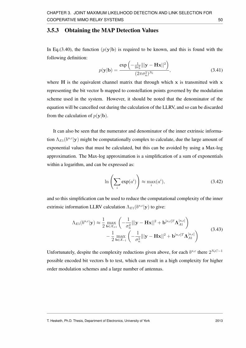
CHAPTER 3. JOINT MAXIMUM LIKELIHOOD DETECTION AND LINK SELECTION FOR
COOPERATIVE MIMO RELAY SYSTEMS 50
3.5.3 Obtaining the MAP Detection Values
In Eq.(3.40), the function (p(y|b) is required to be known, and this is found with the
following definition:
p(y|b) =exp
(− 1
2σ2n‖|y −Hx||2
)(2πσ2
n)Nt, (3.41)
where H is the equivalent channel matrix that through which x is transmitted with x
representing the bit vector b mapped to constellation points governed by the modulation
scheme used in the system. However, it should be noted that the denominator of the
equation will be cancelled out during the calculation of the LLRV, and so can be discarded
from the calculation of p(y|b).
It can also be seen that the numerator and denominator of the inner extrinsic informa-
tion ΛE1(bn,c|y) might be computationally complex to calculate, due the large amount of
exponential values that must be calculated, but this can be avoided by using a Max-log
approximation. The Max-log approximation is a simplification of a sum of exponentials
within a logarithm, and can be expressed as:
ln
(∑i
exp(ai)
)≈ max
i(ai), (3.42)
and so this simplification can be used to reduce the computational complexity of the inner
extrinsic information LLRV calculation ΛE1(bn,c|y) to give:
ΛE1(bn,c|y) ≈ 1
2maxb∈X+1
(− 1
σ2n
‖|y −Hx||2 + b[n,c]TΛ[n,c]A1
)− 1
2maxb∈X−1
(− 1
σ2n
‖|y −Hx||2 + b[n,c]TΛ[n,c]A1
) (3.43)
Unfortunately, despite the complexity reductions given above, for each bn,c there 2NtC−1
possible encoded bit vectors b to test, which can result in a high complexity for higher
order modulation schemes and a large number of antennas.
T. Hesketh, Ph.D. Thesis, Department of Electronics, University of York 2013

CHAPTER 3. JOINT MAXIMUM LIKELIHOOD DETECTION AND LINK SELECTION FOR
COOPERATIVE MIMO RELAY SYSTEMS 51
3.5.4 Cooperative List Sphere Decoder
The cooperative LSD is a variant of the SD, which instead of attempting to reach a single
ML optimal solution, produces a list of the most likely ML solutions, as the solution to
Eq.(3.11) may not be the optimal solution to satisfy Eq.(3.34). If we are given a desired
list size L of list L, then the LSD needs to return L solutions. To this end, we can alter the
procedure of the SD so that if a partial solution satisfying the radius constraint is found,
it is added to L if L is not full, and if L is full, the partial Euclidean distance of the partial
solution is compared to the largest partial Euclidean distance in L, replacing the existing
partial solution if the new partial Euclidean distance is smaller.
When the cooperative LSD has completed its processing, L contains the ML solution
(given that the radius constraint is appropriately large), and theL−1 next closest solutions.
The list L can then be used as a constrained set for Eq.(3.43), reducing the search size for
the max function:
ΛE1(bn,c|y) ≈ 1
2max
b∈L∩X+1
(− 1
σ2n
‖|y −Hx||2 + b[n,c]TΛ[n,c]A1
)− 1
2max
b∈L∩X−1
(− 1
σ2n
‖|y −Hx||2 + b[n,c]TΛ[n,c]A1
) (3.44)
If the size of the list L is set to the maximum possible size 2NtC , then this is equivalent
to full MAP detection, and if L = 1, then this is equivalent to ML detection, as the LSD
will only return the ML solution (assuming appropriate constraint radius size).
It should be noted that for iterations of the iterative MAP detection process, the coop-
erative LSD only relies on the observed received signal vector y and the channel matrix
H, and does not use any extra information from the iterative process, such as the a priori
LLR ΛA1, and so the listLwill not change between iterations on the same y, consequently
the list L can be generated once for the first iteration using the LSD, and used for each
iteration without reprocessing.
T. Hesketh, Ph.D. Thesis, Department of Electronics, University of York 2013

CHAPTER 3. JOINT MAXIMUM LIKELIHOOD DETECTION AND LINK SELECTION FOR
COOPERATIVE MIMO RELAY SYSTEMS 52
3.6 Simulations
In this section, the results of the simulations performed using the techniques set out in
this chapter are presented. In the simulation environment, the assumption is made that
the relays are arranged pseudo-randomly in an area defined by a set of polar coordinates,
i.e. a radius length and an angle, that is centred on the source node which is defined as
being a relative distance of unit 1 for the S to D link for the purposes of the path loss
fading calculations in Eqs.(3.4)-(3.6). The radius length of the polar positioning dsrmis
determined as a uniform random variable between a minimum rmin and maximum radius
rmax limit, and the angular component θsrm is a uniform random angle between 0 and
2π. The distance of the relay nodes to the destination node drdm is then calculated using
trigonometrical identities, as below:
drdm =√d2srm + 1− 2dsrm cos(θsrm) (3.45)
For the numerical results, rmin is set to 0.1 and rmax is set to 0.9. For the power allo-
cation matrices A, the system allocates half of the global power constraint (across both
phases) to the source node, and the other half spread evenly across the relay nodes. The
global power constraint is set to 1 for the obtained results, and so the source node power
allocation matrix As is set as:
As =
√0.5
Nt
I (3.46)
and the relay power allocation matrices Arm are set as:
Arm =
√0.5
NtRL
I (3.47)
If the system is operating without using relay selection (i.e. all relays are used), then the
number of selected relays value RL in Eq.(3.47) is replaced with the number of relays in
the system M . For the fading effects associated with the channel H, the path loss fading
for the channels associated with each relay is defined by the distances dsrm and drdm , and
the base power loss of the S to D link, L. For the simulations, L is set as a 20dB power
loss. The large scale LNS is randomised per packet according to a log-normal random
distribution, with the shadowing spread set at 6dB for all channels.
T. Hesketh, Ph.D. Thesis, Department of Electronics, University of York 2013

CHAPTER 3. JOINT MAXIMUM LIKELIHOOD DETECTION AND LINK SELECTION FOR
COOPERATIVE MIMO RELAY SYSTEMS 53
0 5 10 15 20
10−3
10−2
10−1
100
SNR(dB)
BE
R
No Relays
1 Relay
2 Relays
4 Relays
6 Relays
(a) System model used in this chapter
0 5 10 15 2010
−5
10−4
10−3
10−2
10−1
100
SNR(dB)
BE
R
No Relay
1 Relay
2 Relays
4 Relays
6 Relays
(b) Rayleigh system model commonly used in lit-erature
0 5 10 15 2010
−6
10−5
10−4
10−3
10−2
10−1
100
SNR(dB)
BE
R
No Relays
1 Relay
2 Relays
4 Relays
6 Relays
(c) System model used in [85]
0 5 10 15 20
10−3
10−2
10−1
100
SNR(dB)
BE
R
No Relays
1 Relay
2 Relays
4 Relays
6 Relays
(d) System model used in [89]
Figure 3.5: 2x2 MIMO System, QPSK modulation with a variable number of relays
Within the system, we assume that the channel information is perfectly known at the
relay and destination nodes, and that the relays in the second phase all transmit with per-
fect synchronisation. Fig.3.5a shows the results of a 2x2 MIMO system with no channel
coding or link selection, with a hard decision ML SD detector at the destination, using a
QPSK modulation scheme with Gray coding to minimise bit errors when adjacent sym-
bols are incorrectly detected. The system model used is the model described in Section
II. The number of relays in the system is varied, from no relays (non-cooperative case),
to 6 relays (cooperative case). It can be seen that the addition of a single relay to the
system can improve BER performance by up to 7dB, but the gains of adding extra relays
quickly diminish. Adding two relays to the system gives approximately an extra 2dB of
BER gain, but four relays only give another ∼1dB of gain.
Increasing the number of relays beyond four appears to give no gains, and it can be
T. Hesketh, Ph.D. Thesis, Department of Electronics, University of York 2013

CHAPTER 3. JOINT MAXIMUM LIKELIHOOD DETECTION AND LINK SELECTION FOR
COOPERATIVE MIMO RELAY SYSTEMS 54
observed that for six relays, there is actually a BER performance loss at high values of
SNR as compared to the four relay case. This can be attributed to the relays causing
destructive interference amongst each other, and the power constraint causing the relays
to have less and less transmission power as the number of relays increases. So it can
be seen that if the extra relays do not contribute gains to the BER performance, then a
method of selecting relay links that are beneficial whilst discarding relay links that do
not contribute gains may save resources in the system (such as freeing up relays for other
potential users), and possibly increase the BER gains.
Fig.3.5b represents the BER results for a similar system to Fig.3.5a, but with the sys-
tem model instead having Rayleigh channel modelling, with no path loss or LNS fading,
as is common in literature on cooperative systems. Only the channel modelling is changed
for fair comparison with the system described in this chapter. It can be seen that unlike
Fig.3.5a, adding relays to the system does not appear to contribute much BER gain, until
a high SNR value, and at that point, adding more than one relay does not give much BER
gain.
Fig.3.5c shows the BER results for the channel model and relay placement scheme
from [85], which proposed the single relay cooperative ML detector. This model takes
into account path loss, but the relay(s) are placed very close to the source node, and so is
in an advantageous position. Adding the relays to the system gives a very large BER gain
as the relays are well placed and fixed in position, and so the performance is much greater
than Fig.3.5a.
Fig.3.5d shows the BER results for a system with path loss and 8dB of shadowing,
which is similar to the system model described in this chapter, but the relays are fixed
in position midway between the source and destination nodes, and so are well placed
for relaying signals. The performance is similar to Fig.3.5a, due to the similarity of the
system model used, but the static, well placed relays give this system reliability and a
slight performance gain over Fig.3.5a.
The system models compared and contrasted in Fig.3.5a-d show that the system mod-
els in previous literature tend to not take into account all the features of the system model
described in this chapter, such as the path loss or LNS, or for considering non-static relays,
T. Hesketh, Ph.D. Thesis, Department of Electronics, University of York 2013

CHAPTER 3. JOINT MAXIMUM LIKELIHOOD DETECTION AND LINK SELECTION FOR
COOPERATIVE MIMO RELAY SYSTEMS 55
that may not be well placed for relaying signals.
0 5 10 15 20
10−4
10−3
10−2
10−1
100
SNR(dB)
BE
R
No Link Selection
CP Link Selection
MS−CP Link Selection
MH−CP Link Selection
MM−CP Link Selection
MHC−CP Link Selection
MMC−CP Link Selection
(a) 1 relay link selected
0 5 10 15 20
10−4
10−3
10−2
10−1
100
SNR(dB)
BE
R
No Link Selection
CP Link Selection
MS−CP Link Selection
MH−CP Link Selection
MM−CP Link Selection
MHC−CP Link Selection
MMC−CP Link Selection
(b) 2 relay links selected
0 5 10 15 20
10−4
10−3
10−2
10−1
100
SNR(dB)
BE
R
No Link Selection
CP Link Selection
MS−CP Link Selection
MH−CP Link Selection
MM−CP Link Selection
MHC−CP Link Selection
MMC−CP Link Selection
(c) 3 relay links selected
Figure 3.6: BER vs S → D SNR for the 2x2 MIMO relay system with QPSK modulationand no channel coding with a hard-decision SD, 6 relays, with 1,2 or 3 relay links selectedfor different relay selection schemes
Fig.3.6 shows the comparison of the different relay link selection schemes in a system
with no channel coding or soft information, using the hard decision ML SD for detec-
tion at the destination. The 2x2 MIMO system is using a QPSK modulation scheme with
Gray coding, with 6 relays available in the system. The scenarios presented in Fig.3.6
show the BER versus SNR for 1,2 and 3 relay links being selected from the 6 relays avail-
able in the system. It can be seen that the MH-CP and MM-CP link selection strategies
perform much better than the MS-CP and CP link selection strategies, and the proposed
MHC-CP and MMC-CP outperforms the other link selection strategies. For the single
relay selected case, the proposed combinatorial strategies are seen to perform exactly as
T. Hesketh, Ph.D. Thesis, Department of Electronics, University of York 2013

CHAPTER 3. JOINT MAXIMUM LIKELIHOOD DETECTION AND LINK SELECTION FOR
COOPERATIVE MIMO RELAY SYSTEMS 56
0 2.5 5 7.5 10 12.5 1510
−6
10−5
10−4
10−3
10−2
10−1
100
SNR (dB)
BE
R
No Link Selection
CP Link Selection
MH−CP Link Selection
MHC−CP Link Selection
(a) Rate 1/2 code, generator [7,5]
0 2.5 5 7.5 10 12.5 1510
−6
10−5
10−4
10−3
10−2
10−1
100
SNR (dB)
BE
R
No Link Selection
CP Link Selection
MH−CP Link Selection
MHC−CP Link Selection
(b) Rate 1/3 code, generator [7,7,5]
Figure 3.7: BER vs S → D SNR for the 2x2 channel coded MIMO relay system withQPSK modulation and iterative detection and decoding, 6 relays, 2 relay links selectedand 3 iterations of detection and decoding with a list size of 8 for the LSD
the non-combinatorial versions, as with only 1 relay being selected, there are no combi-
nations as such, and so the combinatorial schemes reduce to the non-combinatorial cases.
For 2 relays selected in the system, the gains of the combinatorial strategies over the
non-combinatorial strategies are seen to be 2-3dB, and similarly for 3 relays selected,
the difference between the non-combinatorial and the combinatorial is ∼3dB. This is ex-
pected for the CP link selection, as this only uses limited channel information from the
system, but the MS-CP strategy has full knowledge, and still has very little gain over the
simpler CP strategy. The performance of the MH-CP and MM-CP link selection strate-
gies is extremely similar for this setup, and so the MM-CP link selection could be seen as
preferable, as it has a lower cost than the MH-CP. The proposed combinatorial MHC-CP
and MMC-CP are seen to provide superior BER performance in the system as compared
to the other link selection strategies considered, but at a higher computational complexity.
Fig.3.7a shows the system with an iterative detection and decoding scheme at the des-
tination and convolutional channel coding at rate 1/2. The 2x2 MIMO system is using
Gray coded QPSK, 6 relays, with 2 relays selected by the link selection methods. The
presented plots are the numerical results from the 3rd iteration of decoding in the iterative
detection and decoding scheme, with a list size of 8 for the LSD. It can be seen that the
CP link selection is not very effective in this system setup, with a slight performance loss
over no link selection scheme being implemented. However, the MH-CP and MHC-CP
schemes have up to 7.5dB and 9dB of gain respectively over no link selection scheme
T. Hesketh, Ph.D. Thesis, Department of Electronics, University of York 2013

CHAPTER 3. JOINT MAXIMUM LIKELIHOOD DETECTION AND LINK SELECTION FOR
COOPERATIVE MIMO RELAY SYSTEMS 57
being used. At higher SNR values, the MHC-CP link selection method has up to 3.5dB
of gain over the non-combinatorial MH-CP link selection scheme. Comparing the coded
system from Fig.3.7a with the uncoded system from Fig.3.6(b), the MH-CP link selection
scheme can been seen to have a decade of BER gain in the coded system over the equiv-
alent uncoded system at 15dB SNR, and similarly the MHC-CP link selection scheme in
the coded system can be seen to have a decade and a half of BER gain over the MHC-CP
link selection scheme in the uncoded system at 15dB SNR. Fig.3.7b represents the results
for the same system setup, but with a rate 1/3 code. The rate 1/3 code can be seen to give
up to 2dB of gain over the rate 1/2 code for the MHC-CP link selection, with the gains
between the different link selection techniques being similar to that for the rate 1/2 code.
In the case of the system setup being simulated for these numerical results, it can be
seen that selecting more than 2 relays out of the 6 available reduces the BER performance
of the harmonic channel power and maximum minimum channel channel power link se-
lection, whilst channel power and sum channel power link selection strategies slightly
increase in performance. This suggests that on average for the relay setup considered,
that only 1-2 relays will be in a position that benefits the transmission from the source to
the relay in terms of BER performance, also considering the power constraint that divides
power between the relays.
3.7 Summary
In this chapter, we have defined a two phase cooperative system incorporating path-loss
based and large scale shadowing based fading, with variable positioning of MIMO AF
relays for a MIMO source and destination under a power constraint. In this system we
have demonstrated cooperative ML detection that incorporates both phases of the received
signal from the source and relays expressed as a single cooperative ML rule that can
be processed by a SD detector, taking into account available information in the system
and making appropriate substitutions so that the results can be numerically calculated.
Also considered is the use of soft decision information and iterative processing for MAP
detection, utilising the LSD as a soft decision detector that can be incorporated into a
channel coded iterative processing detector. Several relay link selection strategies are also
T. Hesketh, Ph.D. Thesis, Department of Electronics, University of York 2013

CHAPTER 3. JOINT MAXIMUM LIKELIHOOD DETECTION AND LINK SELECTION FOR
COOPERATIVE MIMO RELAY SYSTEMS 58
considered for the system, with limited channel information and full channel information
scenarios considered. The proposed combinatorial link selection strategies have been
shown to have BER performance gains over existing link selection schemes in both coded
and uncoded cooperative MIMO systems. It has also been shown that adding relays to
the system may not necessarily give BER gains, depending on the positioning and the
number of relays present in the system model, and so the relay link selection strategies
can be shown to give gains in BER performance over a full relay case, even when using
less relays. It is also shown that some relay link strategies do not necessarily give BER
gains, but it can be considered that the relay link selection can still maintain the BER
performance, whilst releasing some relay resources that could be used by other potential
users.
T. Hesketh, Ph.D. Thesis, Department of Electronics, University of York 2013
Chapter 4
Multi-Feedback Successive Interference
Cancellation with Dynamic Reliability
Ordering
Contents4.1 Introduction . . . . . . . . . . . . . . . . . . . . . . . . . . . . . . . 60
4.2 System Model . . . . . . . . . . . . . . . . . . . . . . . . . . . . . . 61
4.3 Interference Cancellation Techniques . . . . . . . . . . . . . . . . . 62
4.4 Proposed Multiple Feedback Reliability Ordering Successive Inter-
ference Cancellation . . . . . . . . . . . . . . . . . . . . . . . . . . . 69
4.5 Computational Complexity . . . . . . . . . . . . . . . . . . . . . . . 71
4.6 Iterative Detection and Decoding . . . . . . . . . . . . . . . . . . . . 75
4.7 Simulation Results . . . . . . . . . . . . . . . . . . . . . . . . . . . . 78
4.8 Summary . . . . . . . . . . . . . . . . . . . . . . . . . . . . . . . . . 83
T. Hesketh, Ph.D. Thesis, Department of Electronics, University of York
59
2013

CHAPTER 4. MULTI-FEEDBACK SUCCESSIVE INTERFERENCE CANCELLATION WITH
DYNAMIC RELIABILITY ORDERING 60
4.1 Introduction
Successive Interference Cancellation (SIC) detectors [81] are a well known class of de-
tectors for multi-user or multiple-input-multiple-output (MIMO) systems, where upon the
estimation of a data symbol, the estimated data symbol’s effect is removed from the re-
ceived signal in order to improve the signal to interference and noise ratio (SINR) of the
remaining data symbols in that time instant. However, this type of detector can suffer
from error propagation. If the estimated data symbols are not reliable then this unreliabil-
ity can impair all subsequent symbol estimates at a given time instant, degrading the bit
error rate (BER) performance. [9, 68, 72]
A well-known technique for improving the performance of the SIC detector is to re-
move the data streams with the greatest power first, thus removing the greatest source of
interference first, which is known as the VBLAST technique [103], and is implemented
by considering the powers of the channels associated with each user or antenna. However,
as shown in [106], although the VBLAST cancellation order within the SIC is the optimal
for the vast majority of detected symbols, other cancellation orders can outperform the
VBLAST ordering on a given occasion, which could result in performance gains.
In this chapter, dynamic reliability ordering (RO) based upon log-likelihood-ratios
(LLR) [73] is considered in conjunction with a method of multiple-feedback (MF), [107],
[108, 109] which is designed to provide alternative cancellation candidates for data sym-
bols, to compensate for and correct potentially erroneous detected symbols. These meth-
ods are integrated into the proposed MF-RO-SIC detector, which utilises both methods
and makes considerations for reducing the computational complexity associated with
these methods, whilst increasing the BER performance. A discussion on the complexity
of the proposed detector with comparisons to existing methods, and a method for integrat-
ing the proposed detector with iterative detection and decoding in a channel coded system
is also considered.
This chapter is organised as follows, firstly the point-to-point MIMO system model
on which this chapter’s work is based will be described, followed by an in-depth look at
interference cancellation techniques, including SIC, RO and MF techniques, and an ex-
planation of Voronoi diagrams. In the next section, the proposed MF-RO-SIC detector is
T. Hesketh, Ph.D. Thesis, Department of Electronics, University of York 2013

CHAPTER 4. MULTI-FEEDBACK SUCCESSIVE INTERFERENCE CANCELLATION WITH
DYNAMIC RELIABILITY ORDERING 61
detailed, and the integration of the methods involved is developed to produce an algorithm
with reduced computational complexity. After this, an iterative detection and decoding
system for the proposed MF-RO-SIC detector is detailed, which includes a method of hard
decision feedback. Finally, the results of simulations in the point-to-point system model
are presented, for both the proposed detector and the iterative detection and decoding
methods, ending with a summary of this chapters main results.
4.2 System Model
The system under consideration is a point-to-point spatial multiplexing MIMO link, con-
sisting of N transmit antennas and M receive antennas. At each time instant, the N
length column vector x consisting of N data symbols taken from the constellation set
V that is appropriate for the modulation scheme being used, is transmitted through the
M × N channel matrix H. At the M receive antennas at the destination, the transmitted
signal vector is received, processed and organised as the M length column vector y with
sufficient statistics for detection and estimation. This can be described as:
y = Hx + n, (4.1)
where n is the circular complex additive white Gaussian noise (AWGN) vector represent-
ing noise at the receive antennas with a variance given by
σ2 = N/(2γ), (4.2)
where γ is the signal-to-noise ratio (SNR). The channel H is modelled as a complex
Rayleigh distributed channel, and can be expressed as the horizontal concatenation of the
individual channel vector associated with each transmit antenna,
H = [h1, ...,hi, ...,hM ]. (4.3)
The linear MMSE detection technique described in Chapter 2 will be used in this
chapter as the basis for the proposed interference cancellation method developed in this
T. Hesketh, Ph.D. Thesis, Department of Electronics, University of York 2013

CHAPTER 4. MULTI-FEEDBACK SUCCESSIVE INTERFERENCE CANCELLATION WITH
DYNAMIC RELIABILITY ORDERING 62
chapter. The MMSE filter detection can be described as below:
x = Q[WHMMSEy], (4.4)
where x is the N length vector of the estimated transmitted data, which can also be de-
scribed as per-antenna values [x1, . . . , xi, . . . , xM ] and Q[•] represents the quantisation
function appropriate for the modulation scheme being used in the system. It is possible
to estimate the distribution of the bits (bi ∈ −1,+1) of the elements of x as Gaussian
random variables, as shown in [63], with a probability density function (PDF) of:
f(xi|bi) =1√
2πσiexp
[−(xi −mi)
2
2σ2i
], n = 1, ...,M, (4.5)
where mi and σ2i are the mean and variance, respectively,
mi =γi
1 + γibi, (4.6)
σ2i =
γi2(1 + γi)2
, (4.7)
with γi representing the instantaneous SINR of transmit antenna i. The fact that the
elements of x can be accurately modelled as Gaussian random variables is important as
this makes the analysis of the MMSE detection output convenient, thus making it easier
to derive useful results for determining cancellation ordering in later sections.
4.3 Interference Cancellation Techniques
In this section, we shall review the interference cancellation techniques that are involved
in our proposed MF-RO-SIC detector, with an overview of the SIC method with the
VBLAST technique and the importance of the order of interference cancellation, a look
at the idea of dynamic ordering and a method of ordering based on the reliability of es-
timated symbols using the LLR values of the estimated symbols.Finally the technique of
MF is discussed with consideration for computational complexity.
T. Hesketh, Ph.D. Thesis, Department of Electronics, University of York 2013

CHAPTER 4. MULTI-FEEDBACK SUCCESSIVE INTERFERENCE CANCELLATION WITH
DYNAMIC RELIABILITY ORDERING 63
4.3.1 Successive Interference Cancellation
The method of SIC was discussed in Chapter 2, based upon the theory that if in a system
where multiple signals are interfering with each other, if each signal is estimated individ-
ually serially, then the interference effects of an estimated signal can be removed from
the signals that have yet to be estimated, thus increasing the accuracy of estimation of the
remaining signals. The linear MMSE filter detection method is commonly used within
this process over the ZF method, as the MMSE filter gives better BER performance than
ZF, especially at low SNR values.
The order in which a SIC process cancels the estimated signals can make a significant
difference to the overall error rate performance of the detection algorithm, as some signals
will have a greater effect on the level of interference than others. If the signal being esti-
mated has a high level of interference, the symbol estimate produced has a greater chance
of being inaccurate. If this inaccuracy is then used for cancellation in the algorithm, this
may cause the other signals to also be estimated incorrectly, in an effect known as error
propagation.
To reduce the impact of this effect, we can order the signals by the greatest associated
channel power first, and the weakest last, as this ensures that the signals with a good SINR
are estimated first, and are thus less likely to be unreliably estimated. This also means the
interferer with the greatest power is cancelled first, improving the SINR of the remaining
signals by the greatest amount, and this is known as Ordered SIC (OSIC) or the VBLAST
algorithm. In a quasi-static channel environment, this can be calculated once per packet,
and the resultant ordering used for every time instant in that packet.
4.3.2 Log Likelihood Ratio Based Reliability Ordering
As the well-known VBLAST technique is based on the average channel power per an-
tenna, which does not consider the received signal and the effect of noise in a given time
instant, it does not take into consideration the per-time instant fluctuations in SINR at the
receive antennas. The SINR at each antenna is affected by multiple factors, including
the channel state and the random noise at the antennas, as well as other possible inter-
T. Hesketh, Ph.D. Thesis, Department of Electronics, University of York 2013

CHAPTER 4. MULTI-FEEDBACK SUCCESSIVE INTERFERENCE CANCELLATION WITH
DYNAMIC RELIABILITY ORDERING 64
ference effects, such as other transmissions from other systems. Thus, just considering
the channel state once per packet of data transmission, and resorting to an interference
cancellation ordering decision based on this information could lead to accuracy loss when
computing the SIC algorithm. So a possibility for the SIC method is consider the can-
cellation order on a per-time instant basis, possibly resulting in the ordering changing at
each time instant, giving the SIC method a dynamic ordering.
To calculate the dynamic ordering, we could consider the SINR at each time instance,
and directly derive a method to calculate the ordering, however this would likely require
accurate knowledge of the nature of interference, and so could be difficult to obtain. How-
ever, if we consider the LLR at each time instant of transmission, it is possible to derive a
dynamic ordering of the SIC process [73], [110]. First, let us consider the LLR of a bit of
a received symbol given the estimate xi:
Li =
∣∣∣∣ln [f(xi|bi = +1)
f(xi|bi = −1)
]∣∣∣∣ . (4.8)
The magnitude of Li can be considered a measurement of how certain the detector can be
that the estimated symbol is correct when the quantisation of xi is performed, and thus can
be considered a measure of the reliability of the estimated bit. Now, if the filter WMMSE
of the linear MMSE detector is considered:
WMMSE = (HHH + Iσ2n)−1H = R−1
y H, (4.9)
the filter for each individual antenna wi can be rewritten as a product of the auto-
correlation matrix of the interference plus noise Ri:
wi = (1 + hHi R−1i hi)
−1R−1i hi, (4.10)
Ri =
M∑l=1l 6=i
hlhHl + Iσ2
n
. (4.11)
If Eq.(4.10) is substituted into Eq.(4.4), the Gaussian PDF Eq.(4.5) of x can give us the
instantaneous SINR γi as:
γi = hHi R−1i hi. (4.12)
T. Hesketh, Ph.D. Thesis, Department of Electronics, University of York 2013

CHAPTER 4. MULTI-FEEDBACK SUCCESSIVE INTERFERENCE CANCELLATION WITH
DYNAMIC RELIABILITY ORDERING 65
Now, if the Gaussian approximation for xi in Eq.(4.5) is substituted into Eq.(4.8), the
reliability Li is equivalent to:
Li = 4(1 + γi)|xi| ≡ (1 + γi)|xi|. (4.13)
However, γi requires R−1i , which may be complex to acquire in the system. In [110],
the matrix inversion lemma may be applied to R−1n , resulting in:
γi =hHi R−1
y hi
1− hHi R−1y hi
, (4.14)
which only uses R−1y , which is already obtained for use in the MMSE filter. Substituting
this result into Eq.(4.13) and simplifying gives:
Li = (1− hHi R−1y hi)
−1|xi|, (4.15)
which is referred to as the Type-L reliability [110] for bi. If we are using a modula-
tion scheme with multiple bits per symbol (for example Quadrature Phase Shift Keying
(QPSK)), then a simple extension to Eq.(4.15) is:
Li = (1− hHi R−1y hi)
−1(|<(xi)|+ |=(xi)|). (4.16)
This reliability Li can be incorporated into the SIC algorithm, as at every stage of the
SIC procedure for each antenna’s signal that has not yet been estimated, the reliability
can be calculated, and the signal with the highest reliability measurement will be the next
estimated signal. This results in a dynamic ordering that is not predetermined before the
SIC is processed, and can change with every time instant. Table 4.1 shows the algorithm
used for the RO-SIC process.
4.3.3 Multiple Feedback Cancellation
The method of MF [107–109] in a SIC process is based on the idea of reliable and unre-
liable symbol estimates, and how alternative symbol quantisation decisions can affect the
cancellation results. During the SIC cancellation process, the quantised estimated symbol
T. Hesketh, Ph.D. Thesis, Department of Electronics, University of York 2013

CHAPTER 4. MULTI-FEEDBACK SUCCESSIVE INTERFERENCE CANCELLATION WITH
DYNAMIC RELIABILITY ORDERING 66
Table 4.1: Reliability Ordering Successive Interference Cancellation Algorithm
Initialisation: y0 = y,H0 = H, Ry,0 = HHH + Iσ2n
for i = 1→ N doWi = R−1
y,i−1Hi−1
xi = WHi yi−1
for j = 1→ (N + 1− i) doLj = (1− hHj R−1
y,i−1hj)−1|xj |
end forj = argmaxLj (L1, ..., LN+1−i)xj = Q[xi(j)]yi = yi−1 − xjhjHi = H′i−1
〈j〉
Ry,i = Ri−1 − hjhHj
end for
xn, is defined as xi = Q[xi], where Q[] is the quantisation function appropriate for the
modulation scheme being used in the system, and the quantisation operates by choosing
the constellation point c with the smallest Euclidean distance to the estimated symbol as
described by
xi = arg minc∈V‖xi − c‖2. (4.17)
Figure 4.1: Example of a Voronoi diagram
This operation can be represented by a Voronoi diagram [111–113], which is a method
of dividing an area up into regions around a set of points placed in the area. Each point
in the diagram has a Voronoi cell associated with it, and the area within each Voronoi cell
T. Hesketh, Ph.D. Thesis, Department of Electronics, University of York 2013

CHAPTER 4. MULTI-FEEDBACK SUCCESSIVE INTERFERENCE CANCELLATION WITH
DYNAMIC RELIABILITY ORDERING 67
is defined as the space which has the Voronoi cell’s point as its closest point in Euclidean
distance. Fig. 4.1 shows an example of a Voronoi diagram with 6 points on a flat plane.
The area is divided up into 6 regions around the 6 points, and if any position on the plane
is chosen, the region in which the position is located shows which point is closest. The
boundaries between the Voronoi regions can be called Voronoi boundaries, and represent
the threshold at which a position can be considered to be close to two or more points.
The Voronoi diagram can thus be shown to correspond to how the quantisation function
quantises estimated symbols to constellation points on a constellation diagram, with the
Voronoi points representing the constellation points, the Voronoi regions showing where
an estimated symbol will be quantised to and the Voronoi boundaries showing where the
decision boundaries are located. Fig. 4.2a and 4.2b show the Voronoi diagrams for QPSK
and 16-QAM modulation schemes, and so show how estimated symbols will be quantised.
I
Q
00
1011
01
(a) QPSK
I
Q
0011
00010000
0010
0101
0111
0100
0110
1010
1000
1011
1001
1101 1100
11101111
I
Q
0011
00010000
0010
0101
0111
0100
0110
1010
1000
1011
1001
1101 1100
11101111
(b) 16-QAM
Figure 4.2: Voronoi diagrams for QPSK and 16-QAM modulation schemes
However, if the estimated symbol is close to the Voronoi boundaries of two or more
constellation points, then the estimated symbol could conceivably be attributed to a con-
stellation point that does not have the smallest Euclidean distance from the estimated
symbol, as the effects of noise and interference are likely to cause the estimate to cross a
Voronoi boundary.
Therefore, an area surrounding the Voronoi boundaries can be described as a scenario
in which is it possible that the standard quantisation process may give inaccurate results.
And so, a shadowing region on the constellation diagram is created, which defines an area
T. Hesketh, Ph.D. Thesis, Department of Electronics, University of York 2013

CHAPTER 4. MULTI-FEEDBACK SUCCESSIVE INTERFERENCE CANCELLATION WITH
DYNAMIC RELIABILITY ORDERING 68
in which an estimated symbol may be considered for alternative quantisation results. If
xi falls within this region, then the C alternative constellation points with the smallest
Euclidean distances (U ⊂ V, [u1, ..., uC ]) to xi are considered for SIC processing, instead
of just the closest. Fig. 4.3 shows how the shadowing region is defined by a shadowing
criterion value S for QPSK modulation, which defines how far from the constellation axes
(which are the Voronoi boundaries for a QPSK constellation) the shadowing region is set.
ℑ
ℜ
Constellation PointSVoronoi Boundaries
Figure 4.3: Shadow region for QPSK modulation
When these alternative candidates for xi are considered, the MF algorithm processes
the SIC to completion for the C possible candidates, to produce an estimated symbol
vector for all transmitted antennas xc, c = 1, ..., C. Then using the ML rule, the MF
technique chooses the xc that produces the smallest Euclidean distance as described by:
x = arg min‖y −Hxc‖2, c = 1, ..., C. (4.18)
The symbol candidate uc associated with the chosen xc is then chosen as xi for that
cancellation stage, and the MF-SIC continues from the ith stage. Table 4.2 shows the
MF-SIC algorithm.
T. Hesketh, Ph.D. Thesis, Department of Electronics, University of York 2013

CHAPTER 4. MULTI-FEEDBACK SUCCESSIVE INTERFERENCE CANCELLATION WITH
DYNAMIC RELIABILITY ORDERING 69
Table 4.2: Multiple Feedback Successive Interference Cancellation Algorithm
Initialisation: y0 = y,H0 = Hwi = (HiH
Hi + Iσ2
n)−1hi, i = 1, ..., N
for i = 1→ N doxi = wH
i yi−1
if |<[xi]| and |=[xi]| > S thenxi = Q[xi]
elsefor k = 1→ C do
xk = xyki = yi−1 − ukhifor l = i+ 1→ N do
xkl = Q[wHl ykl−1]
ykl = ykl−1 − xkl hlend for
end forxi = argmink=1,...,C‖y −H0xk‖2
end ifyi = yi−1 − xihiHi = H′i−1
〈i〉
end for
Hi represents the matrix formed by taking the columns i, i+ 1, ..., N of H
4.4 Proposed Multiple Feedback Reliability Ordering
Successive Interference Cancellation
Our proposed MF-RO-SIC detector combines the ideas of dynamic ordering within the
SIC process, the multiple candidates feature for unreliable cancellation estimates, and
overcomes the drawbacks of existing SIC detectors by minimising the extra computational
complexity required.
A possibility for the combination of the MF-SIC and RO-SIC is to have the MF process
taking place after the RO algorithm has decided which signal to estimate for this current
iteration of the main SIC for loop. But, as may be noted in the algorithm in Table 4.2, the
MF-SIC adds only a small amount of extra complexity over the SIC, as the cancellation
filters for each stage Wn can be precalculated and reused within the MF process:
wi = (HiHHi + Iσ2)−1hi, i = 1, ..., N, (4.19)
T. Hesketh, Ph.D. Thesis, Department of Electronics, University of York 2013

CHAPTER 4. MULTI-FEEDBACK SUCCESSIVE INTERFERENCE CANCELLATION WITH
DYNAMIC RELIABILITY ORDERING 70
eliminating the requirement to use a matrix inverse at each stage for a filter calculation,
but this is only true if the cancellation order is known before the SIC is processed. In
the case of the RO-SIC, the ordering dynamically changes with each cancellation stage
so that the order is not predetermined, and so the MF filters cannot be precalculated for
each time instant. For this reason, the filters would have to be recalculated for each stage
in the MF, introducing a matrix inversion operation at each cancellation stage, every time
xi falls within the MF shadowing region, as well as determining the dynamic RO. This
would involve a large increase in complexity over the standard MF-SIC, and this should
be avoided.
In order to avoid this large increase in required complexity, we can split the MF-RO-
SIC into two sections. Firstly, the RO-SIC can be calculated as in Table 4.1, in order to
give a base estimate of x, but the cancellation order taken by the dynamic ordering for
this time instant can also be extracted from the algorithm.
RO-SICy
MF-SICx
CancellationOrder
Figure 4.4: Structure of piece-wise MF-RO-SIC
This returned ordering can then be used as a predetermined ordering for the MF-SIC
process, and so the filters can be precalculated as in Table 4.2, with the new predetermined
ordering, which means the filters only have to be calculated once per time instant for the
MF-SIC, reducing the complexity of the MF-SIC process to the original level. This piece-
wise approach is shown in Fig.4.4.
This piece-wise approach to the MF-RO-SIC does save complexity over the exhaustive
ordering algorithm, but the filters are still calculated for the MF-SIC, and in effect the
complexity of the RO-SIC and the MF-SIC is additive, roughly doubling the complexity
over either individual algorithm.
However, greater reductions in complexity can be achieved by further integrating the
two stages together intelligently. The MF-SIC filters gi can be extracted from each stage
of the RO-SIC, by taking and storing the jth column of the RO-SIC filter associated with
the chosen cancellation, thus these values can be reused for the MF-SIC, so that the filters
do not need to be calculated at all for the MF-SIC, reducing the complexity as no extra
T. Hesketh, Ph.D. Thesis, Department of Electronics, University of York 2013

CHAPTER 4. MULTI-FEEDBACK SUCCESSIVE INTERFERENCE CANCELLATION WITH
DYNAMIC RELIABILITY ORDERING 71
matrix inversions have to be performed. The MF-SIC filter gi is given by:
gi = wi,j, (4.20)
where wi,j is the jth column of the filter W calculated for the ith cancellation stage of
the RO-SIC. Also, whilst the MF-SIC cannot be directly integrated into the RO-SIC with
low complexity due to the dynamic ordering restriction, the shadow criterion test for each
xi can still be carried out within the RO-SIC process, as below:
|<[xi]| < S and |=[xi]| < S (4.21)
If no xi falls within the shadow criterion area during the RO-SIC, then logically the
MF-SIC will not give a different x than the RO-SIC, as the MF technique will never be
performed, and so the MF-SIC stage can be skipped for that time instant, reducing com-
plexity further. Fig. 4.5 shows the structure of the MF-RO-SIC with these considerations,
and Table 4.3 shows the complete algorithm for the proposed MF-RO-SIC detector.
RO-SIC Unreliable?y x No
Yes
MF-SIC
x
CancellationOrder, W
Figure 4.5: Structure of proposed MF-RO-SIC
4.5 Computational Complexity
The proposed MF-RO-SIC MIMO detector was designed in the previous section to reduce
the extra complexity required as compared to the methods which the proposed detector
is derived from. In order to fairly compare the algorithms in terms of computational
complexity, it is required that the four methods (SIC, RO-SIC, MF-SIC and MF-RO-SIC)
are analysed in terms of the number of complex additions and multiplications (collectively
called operations) that are needed to run the algorithms per time instant.
T. Hesketh, Ph.D. Thesis, Department of Electronics, University of York 2013

CHAPTER 4. MULTI-FEEDBACK SUCCESSIVE INTERFERENCE CANCELLATION WITH
DYNAMIC RELIABILITY ORDERING 72
Table 4.3: Multiple Feedback Reliability Ordering Successive Interference CancellationAlgorithm
Initialisation: y0 = y,H0 = H, Ry,0 = HHH + Iσ2n,m = 0
for i = 1→ N
Wi = R−1y,i−1Hi−1
xi = WHi yi−1
for j = 1→ (N + 1− i)Lj = (1− hHj R−1
y hj)−1|xj |
end forj = argmaxLj (L1, ..., LN+1−i)gi = wi,j
xj = Q[xi(j)]if |<[xi(j)]| or |=[xi(j)]| < S
m = 1end ifyi = yi−1 − xjhjHi = H′i−1
〈j〉
Ry,i = Ri−1 − hjhHj
end forif m = 1
for i = 1→ Nxi = gHi yi−1
if |<[xi] and |=[xi] > Sxi = Q[xi]
elsefor k = 1→ C
xk = xyki = yi−1 − ukhifor l = i+ 1→ N
xkl = Q[gHl ykl−1]
ykl = ykl−1 − xkl hlend for
end forkopt = argmink=1,...,C‖y0 −H0xk‖2xi = ukopt
end ifyi = yi−1 − xihiHi = H′i−1
〈i〉
end forend if
T. Hesketh, Ph.D. Thesis, Department of Electronics, University of York 2013

CHAPTER 4. MULTI-FEEDBACK SUCCESSIVE INTERFERENCE CANCELLATION WITH
DYNAMIC RELIABILITY ORDERING 73
As the MF-SIC and MF-RO-SIC use the conditional shadow criterion, directly
analysing the complexity will be extremely difficult as the probability of the operations
dependent on the shadow criterion result being run will change with each time instant.
To easily assess the computational complexity, the complexity analysis will include some
empirical variables, which are obtained by running simulations of the algorithms to be
analysed in the system model detailed in Section 4.2. These empirical variables negate
the need for complex statistical analysis of the conditional portions of the algorithms, and
will defined as follows:
• S will represent the average number of shadow criterion tests that are failed (i.e. .
alternative candidates are considered) per time instant.
• T will represent the average number of alternative candidates that are calculated per
time instant.
• Z will represent the average percentage of time instants that require the MF section
of the MF-RO-SIC to be processed.
Using these variables, it is possible to express the computational complexity of the four
methods as shown in Table 4.4, and form comparisons of the relative computational cost.
For the purpose of this analysis, it has been assumed that for matrix inversion operations
that the Gauss-Jordan elimination method has been used. For practical systems, more
efficient methods may be used, but this has little impact on the relative complexity of the
algorithms as each method requires N inversions of an M ×M matrix per time instance
to operate.
Fig. 4.6 shows plots of the computational complexity for different sizes of a MIMO
system, and over different SNR values. For these simulations, QPSK was used as the
modulation scheme, with the shadow criterion S set to 0.2, and the number of alternative
candidates considered C to 4. Fig. 4.6a shows how the complexity changes as the size of
the MIMO system increases, at an SNR of 10dB. It can be seen that adding the MF method
to the SIC and RO-SIC adds very little complexity compared to the original methods, and
that using the RO method roughly doubles the complexity as compared to the SIC. This
is due to the amount of reliabilities that have to be calculated per time instant for the RO
method. Fig. 4.6b shows how the complexity varies over a range of SNR values for a
T. Hesketh, Ph.D. Thesis, Department of Electronics, University of York 2013

CHAPTER 4. MULTI-FEEDBACK SUCCESSIVE INTERFERENCE CANCELLATION WITH
DYNAMIC RELIABILITY ORDERING 74
Table 4.4: Computational Complexity of Interference Cancellation Algorithms
Algorithm Complex Additions Complex Multiplications
SIC N2 (M
2N + 3M2 + 2M − 2) +
N(M3
3 + M2
2 − 5M6 )
MN2 (MN + 3M + 4) +N(M
3
3 +
M2
2 + M3 )
RO-SIC MN2 (5MN − 4N + 5M + 2) +
+N(M3
3 + M2
2 − 5M6 )
N2 (3M
2N + 3MN +N + 5M2 +
3M + 1) +N(M3
3 + M2
2 + M3 )
MF-SIC N2 (M
2N +3M2+2M −2)+N(M3
3 +
M2
2 − 5M6 ) + T (2M − 1) + CM2S
MN2 (MN + 3M + 4) +N(M
3
3 +
M2
2 + M3 ) +M(2T + CMS)
MF-RO-SIC MN2 (5MN − 4N + 5M + 2) +
+N(M3
3 + M2
2 − 5M6 ) + T (2M − 1) +
CM2S + Z(2M − 1)
N2 (3M
2N + 3MN +N + 5M2 +
3M + 1) +N(M3
3 + M2
2 + M3 ) +
M(2T + CMS + 2Z)
2x2 3x3 4x4 5x5 6x6 7x7 8x8
102
103
104
Tx x Rx
Com
ple
x O
pera
tions
SIC
RO−SIC
MF−SIC
MF−RO−SIC
(a) SNR = 10dB, variable MxN
0 5 10 15 20500
750
1000
1250
1500
1750
2000
SNR(dB)
Com
ple
x O
pera
tions
SIC
RO−SIC
MF−SIC
MF−RO−SIC
(b) M,N = 4, variable SNR
Figure 4.6: Number of complex operations for each algorithm for a QPSK MIMO system,S = 0.2, C = 4
4x4 system. The only terms dependent on the SNR are the empirical variables obtained
(S, T and Z), and so the SIC and RO-SIC have no variance in their complexity over the
SNR range, whereas the MF-SIC and MF-RO-SIC do have some variance. At high SNR
values, the MF-SIC and MF-RO-SIC converge towards the SIC and RO-SIC complexity
costs, respectively, due to the shadow criterion test failing only rarely. At low SNR values,
the difference between the MF and non-MF methods can be seen, but the increase in
complexity is only a small percentage. Table 4.5 shows the average percentage increase
in complexity between the RO-SIC and proposed MF-RO-SIC algorithm. At a 0dB SNR,
the MF-RO-SIC only increases the complexity by 2.4%, whereas at 20dB SNR, the MF
section of the algorithm is processed so rarely, that the increase is less than a hundredth
T. Hesketh, Ph.D. Thesis, Department of Electronics, University of York 2013

CHAPTER 4. MULTI-FEEDBACK SUCCESSIVE INTERFERENCE CANCELLATION WITH
DYNAMIC RELIABILITY ORDERING 75
Table 4.5: Average Complexity Cost for RO-SIC and MF-RO-SIC
SNR RO-SIC Operations MF-RO-SIC Operations Average % Increase0 1588.7 1627.3 2.42885 1588.7 1607.1 1.157610 1588.7 1592.6 0.245915 1588.7 1589.1 0.026620 1588.7 1588.8 0.0036
of a percent.
4.6 Iterative Detection and Decoding
Here a hard decision feedback IDD system is presented, incorporating the idea of IDD
[39,98,99,101] with the proposed MF-RO-SIC detector to improve the BER performance
in conjunction with channel coding.
4.6.1 Hard Decision Feedback System
In this scenario, the IDD system is based upon the IDD system in Chapter 3, but in con-
trast, hard decision detection and feedback are used for the detectors, eliminating the
need for a list based MAP algorithm. In the proposed MF-RO-SIC algorithm, the quan-
tised estimated symbols x are used to refine the received signal to increase the accuracy
of subsequent stream detections, but the effectiveness of this interference cancellation is
dependent on the accuracy of the x symbols being cancelled. If the accuracy of x can be
improved, then the BER performance of the MF-RO-SIC detector will improve.
To this end, we can use the detected and decoded bits from an iterative detection system
as a substitute for x in the interference part of a SIC algorithm. The theory behind this
idea is that by using channel coding in the IDD system, the estimated decoded bits will
have a higher accuracy than the encoded bits that are manipulated and estimated between
the encoder stage at the transmitter and the decoder stage at the receiver of the IDD
system. Thus, the symbols derived from the decoded bits will have a better BER than
the x symbols in the MF-RO-SIC algorithm. And so the system consists of the layout
T. Hesketh, Ph.D. Thesis, Department of Electronics, University of York 2013

CHAPTER 4. MULTI-FEEDBACK SUCCESSIVE INTERFERENCE CANCELLATION WITH
DYNAMIC RELIABILITY ORDERING 76
as seen in Fig. 4.7, with the subscripts 1 and 2 representing the inner and outer coding
and mapping functions respectively and ΛD represents the a posteriori LLRV of the inner
bits b of the bit vector b, ΛA is the a priori LLRV of b, ΛE is the extrinsic information
LLRV and the output LLRV ΛO, which is the output of each iteration that is used for the
bit estimation.
Binary Source Encoder Interleaver Costellation
MF-RO-SICDeinterleaverDecoderBit Decision
Estimated Encoder Interleaver SICBinary Data
Mapper
H
y1
b2 λ2 λ1
x1
x1b2
ConstellationMapper
b2 λ2 λ1 x1
x1
ΛD2
DemapperΛD1
ΛA2
InterleaverΛE2 ΛA1
ΛO
Figure 4.7: Hard decision iterative decoding system layout
The binary source bits b2 are first encoded by the channel coding scheme used by the
IDD system (in this case a convolutional code) to produce the outer coded bits λ2, which
are then interleaved into the inner coded bits λ1. The inner coded bits are then mapped
to a constellation diagram to produce the symbols for MIMO transmission x1. The coded
transmitted symbols are received as the received coded signal vector y1, and then the
proposed MF-RO-SIC detectors performs the algorithm to produce the inner estimated
coded transmitted symbols x1. The demapper then will estimate the inner a posteriori bit
LLRV ΛD1 using a MAP method and then this result is deinterleaved to the outer a priori
LLRV ΛA2, which is given to the decoder which produces the output LLRV ΛO. A bit
decision process then takes place on ΛO to produce the outer estimated binary data bits
b2, which is our result for this first iteration of detection.
Now two types of feedback take place, firstly in a similar fashion to Chapter 3’s IDD
system, the decoder also produces the outer a posteriori bit LLRV ΛD2, which has the
ΛA2 subtracted from it to give the outer extrinsic information LLRV ΛE2. This is then
interleaved to give the inner a priori LLRV ΛA1, which is an input to the demapper for
the next iteration of processing.
T. Hesketh, Ph.D. Thesis, Department of Electronics, University of York 2013

CHAPTER 4. MULTI-FEEDBACK SUCCESSIVE INTERFERENCE CANCELLATION WITH
DYNAMIC RELIABILITY ORDERING 77
Secondly, in order to refine the estimated binary data bits, we now feedback these bits
to the SIC algorithm for a refinement of the estimated symbols x1, but this first requires
some manipulation. The outer estimated binary data bits are re-encoded and interleaved
using the same convolutional code and interleaver as the transmitter, to produce the es-
timated inner coded bits λ1, which are then constellation mapped to the estimated inner
coded transmitted symbols x1. A standard SIC detector will then use this re-encoded
result in place of the quantised estimated symbols Q[xi] in the SIC process. The SIC
process will then produce the inner estimated coded transmitted symbols x1 instead of
the MF-RO-SIC, which then are processed in the second iteration as in the first iteration.
Each iteration subsequently is processed using the same method as the second iteration,
producing refined and more accurate versions of b2.
4.6.2 Demapping Estimated Symbols
The demapper in Fig. 4.7 is a two-stage process that relies on the MAP method to pro-
duce individual bit LLRVs from the estimated symbols x1. A difference from the MAP
method in Chapter 3 is that the MAP method here will not have a list of potential symbols
candidates produced by the detector, but only a single vector. In order to calculate the
MAP, the probability of getting the estimate x1 for each possible constellation point is
required. This probability is calculated by:
p(x1|xk) =1
2πσ2exp
(−|x1 − xk|22σ2
), k = 1...K, (4.22)
where K is the number of constellation points in the modulation scheme used, and xk
is the kth symbol in the modulation scheme. To get the symbol likelihood this is then
arranged as:
logf(x1|xk) =−|x1 − xk|2
2σ2, k = 1...K. (4.23)
To obtain the inner bit LLRV Λ1,b, where b is the bit index for each symbol, b = 1...log2K,
we use the above result in a MAP algorithm [114]:
Λ1,b = log
∑xk∈X1
f(x1,b|xk)p(xk)∑xk∈X0
f(x1,b|xk)p(xk)
, (4.24)
T. Hesketh, Ph.D. Thesis, Department of Electronics, University of York 2013

CHAPTER 4. MULTI-FEEDBACK SUCCESSIVE INTERFERENCE CANCELLATION WITH
DYNAMIC RELIABILITY ORDERING 78
where p(xk) is the a priori probability of xk, which is obtained from the decoder after
each iteration. For the first iteration process this is set to 0 for all symbols. The MAP can
then be approximated using the Max-Log approximation detailed in Chapter 3 to give:
Λ1,b ≈ maxxk∈X1
log (f(x1,b|xk)p(xk))− maxxk∈X0
log (f(x1,b|xk)p(xk)) (4.25)
4.7 Simulation Results
For the simulation results presented in this chapter, a MIMO system was considered with
either a QPSK or a 16-QAM scheme, and with perfect knowledge of the channel state
information, the SIC detectors considered are based upon linear MMSE filtering, and the
individual channel elements are modelled as having Rayleigh distributions. Extensions to
other modulation schemes and propagation channels is straightforward.
4 6 8 10 12 14 16 18 2010
−7
10−6
10−5
10−4
10−3
10−2
10−1
100
SNR(dB)
BE
R
VBLAST−SIC
MF−SIC
RO−SIC
MF−RO−SIC
ML
Figure 4.8: 4x4 MIMO with QPSK modulation, C = 4, S = 0.2
Fig. 4.8 shows how the proposed MF-RO-SIC detector compares with the VBLAST-
SIC, RO-SIC, MF-SIC and the ML detector in terms of BER in a 4x4 MIMO system. The
number of candidates for the MF (C) is set to 4, with the shadow criterion S set to 0.2.
The MF-RO-SIC can be seen to have up to 4dB in BER performance improvement over
the MF-SIC, just over 4dB over the RO-SIC and up to 8dB of gain over the VBLAST-SIC.
T. Hesketh, Ph.D. Thesis, Department of Electronics, University of York 2013

CHAPTER 4. MULTI-FEEDBACK SUCCESSIVE INTERFERENCE CANCELLATION WITH
DYNAMIC RELIABILITY ORDERING 79
In this scenario, it appears that the MF method is the major contributor to the MF-RO-SIC
detectors performance in the lower SNR region, with the dynamic RO providing the extra
gains at the higher SNR level.
0 2 4 6 8 10 12 14 1610
−7
10−6
10−5
10−4
10−3
10−2
10−1
100
SNR(dB)
BE
R
VBLAST−SIC
MF−SIC
RO−SIC
MF−RO−SIC
ML
Figure 4.9: 8x8 MIMO with QPSK modulation, C = 4, S = 0.2
Fig. 4.9 similarly shows how the proposed MF-RO-SIC detector compares with the
VBLAST-SIC, RO-SIC, MF-SIC and the ML detector in terms of BER in an 8x8 MIMO
system. The number of candidates for the MF (C) is set to 4, with the shadow criterion
S set to 0.2. The MF-RO-SIC can be seen to have up to 4dB BER performance over the
MF-SIC, just over 2dB over the RO-SIC and up to 8dB of gain over the VBLAST-SIC,
with the MF-RO-SIC approaching the ML performance with a 2dB loss at a high SNR.
It can be noted that in Fig. 4.8, the MF-SIC had better performance than the RO-SIC,
but in Fig. 4.9, the RO-SIC outperformed the MF-SIC, suggesting that for larger MIMO
systems, the RO in the MF-RO-SIC provides the major contribution to the performance
gains of the MF-RO-SIC over the VBLAST SIC, whilst for smaller MIMO systems, the
MF provides the greater performance gains.
Fig. 4.10 shows how the BER performance of the MF-RO-SIC changes as the shadow
criterion is varied, as compared to the RO-SIC and the ML solution. As the shadow
criterion is increased, the BER performance varies from the RO-SIC performance and
tends towards the ML performance. It can be seen that for each 0.1 increase of S, the
BER performance of the MF-RO-SIC has another 1-2dB of gain added. This however, is
T. Hesketh, Ph.D. Thesis, Department of Electronics, University of York 2013

CHAPTER 4. MULTI-FEEDBACK SUCCESSIVE INTERFERENCE CANCELLATION WITH
DYNAMIC RELIABILITY ORDERING 80
0 4 8 12 16 2010
−5
10−4
10−3
10−2
10−1
SNR(dB)
BE
R
RO−SIC
MF−RO−SIC − S 0.1
MF−RO−SIC − S 0.2
MF−RO−SIC − S 0.3
ML
Figure 4.10: 4x4 MIMO with QPSK modulation, C = 4, variable S
at the cost of complexity, as the larger the shadow criterion, the more likely an estimated
symbol is to fall within the shadow area, and thus the MF process is calculated more
often. It should be noted that a degradation in BER performance was observed if S was
set too high (∼ 0.4 > S). This is possibly due to the MF-RO-SIC testing a large amount
of alternative constellation points in the MF process, increasing the likelihood that false
positive solutions are found for the ML rule due to noise and self-interference.
8 10 12 14 16 18 20 22 2410
−6
10−5
10−4
10−3
10−2
10−1
100
SNR(dB)
BE
R
VBLAST−SIC
MF−SIC
RO−SIC
MF−RO−SIC
ML
Figure 4.11: 4x4 MIMO with 16-QAM modulation, C = 4, S = 0.1
Fig. 4.11 shows the performance of proposed MF-RO-SIC detector as compared with
T. Hesketh, Ph.D. Thesis, Department of Electronics, University of York 2013

CHAPTER 4. MULTI-FEEDBACK SUCCESSIVE INTERFERENCE CANCELLATION WITH
DYNAMIC RELIABILITY ORDERING 81
the VBLAST-SIC, RO-SIC, MF-SIC and the ML detector in terms of BER in a 4x4 MIMO
system, in a system using 16-QAM. The number of candidates for the MF (C) is set to 4,
with the shadow criterion S set to 0.1. The shadow criterion is set lower for 16-QAM than
QPSK, as the constellation points for 16-QAM are closer together than for QPSK, and so
the shadow criterion is scaled down to account for this. For this system, the MF-RO-SIC
has 1dB of gain over the MF-SIC, 4dB of gain over the RO-SIC and up to 6dB of gain over
the VBLAST-SIC. The MF-RO-SIC has about 4dB of loss from the ML detector, which
is a greater loss than for QPSK, which suggests that the shadow criterion and number of
candidates can be further optimised.
12 14 16 18 20 22 2410
−4
10−3
10−2
10−1
SNR(dB)
BE
R
RO−SIC
MF−RO−SIC, Shadow 0.05
MF−RO−SIC, Shadow 0.1
MF−RO−SIC, Shadow 0.15
MF−RO−SIC, Shadow 0.2
MF−RO−SIC, Shadow 0.25
Figure 4.12: 4x4 MIMO with 16-QAM modulation, C = 4, variable S
Fig. 4.12 shows the BER performance of the proposed MF-RO-SIC detector as the
shadow criterion is varied. It can be seen that increasing the shadow criterion increases
the BER performance, until at S = 0.15 the performance starts decreasing, as the number
of false positives starts degrading the accuracy of the detector. The value at which the
shadow criterion increase degrades performance is smaller than for QPSK, due to the
smaller separation between the constellation points and the Voronoi boundaries.
Fig. 4.13 shows how varying the candidate limit C affects the BER performance of
the MF-RO-SIC for a 16-QAM modulation. It can be seen that adding extra candidates
(which increases the complexity of the MF section of the algorithm) beyond 4 candidates
T. Hesketh, Ph.D. Thesis, Department of Electronics, University of York 2013

CHAPTER 4. MULTI-FEEDBACK SUCCESSIVE INTERFERENCE CANCELLATION WITH
DYNAMIC RELIABILITY ORDERING 82
12 14 16 18 20 22 2410
−4
10−3
10−2
10−1
SNR(dB)
BE
R
MF−RO, C = 2
MF−RO, C = 4
MF−RO, C = 6
MF−RO, C = 8
Figure 4.13: 4x4 MIMO with 16-QAM modulation, variable C, S = 0.1
8 10 12 14 16 18 2010
−6
10−5
10−4
10−3
10−2
10−1
SNR(dB)
Co
de
d B
ER
SIC− Iteration:1
RO−SIC− Iteration:1
MF−SIC− Iteration:1
MF−RO−SIC− Iteration:1
SIC− Iteration:3
RO−SIC− Iteration:3
MF−SIC− Iteration:3
MF−RO−SIC− Iteration:3
Figure 4.14: 4x3 MIMO with QPSK modulation, C = 4, S = 0.2
has diminishing gains. The gain from using 2 candidates to 4 candidates is approximately
1dB, but the gain from 4 to 6 candidates is less than 0.5dB, similarly from 6 to 8 candi-
dates. This suggests that for this scenario, a choice of 4 candidates in the MF algorithm
offers a very attractive complexity to gain ratio.
Fig. 4.14 shows how the hard decision iterative feedback version of the proposed
T. Hesketh, Ph.D. Thesis, Department of Electronics, University of York 2013

CHAPTER 4. MULTI-FEEDBACK SUCCESSIVE INTERFERENCE CANCELLATION WITH
DYNAMIC RELIABILITY ORDERING 83
MF-RO-SIC performs in terms of coded BER, in a 4x3 MIMO QPSK system. The plots
shown are the results of the 1st and 3rd iteration of decoding and detection. It can been
seen that the 3rd iteration of the MF-RO-SIC outperforms the 3rd iteration of the MF-SIC
by up to 4dB, and the 3rd iteration of the RO-SIC by up to 6dB. It can also be seen that
from the 1st to 3rd iteration of the hard decision feedback system, the MF-RO-SIC gains
up to 3.5dB in BER performance.
4.8 Summary
In this chapter, a new MF-RO-SIC detector has been proposed, utilising the ideas of dy-
namic cancellation stage reliability ordering and multiple candidates for estimated symbol
decisions, with consideration given to the complexity of the resultant detector and how
this can be reduced. An analysis of the complexity shows that the proposed detector adds
very little complexity to the RO-SIC, but that simulation results have shown up to 4dB
of gains over previously established SIC detectors and 8dB gains over the VBLAST-SIC,
for 4x4 and 8x8 MIMO systems with QPSK modulation, and up to 4dB of gain over es-
tablished detectors for a 16-QAM modulation scheme system. It has also been shown
how the BER performance of the MF-RO-SIC detector is altered as the parameters of
the detector are altered, and how this can approach the ML detector performance. Also
considered is an iterative version with channel decoding, utilising hard feedback that is
re-encoded to provide greater accuracy for the interference cancellation process. It is seen
that this IDD method is effective in accurately detecting the transmitted data.
T. Hesketh, Ph.D. Thesis, Department of Electronics, University of York 2013

Chapter 5
Multi-Branch Interference Cancellation
with Widely-Linear Processing for
Multiuser Cooperative MIMO Systems
Contents5.1 Introduction . . . . . . . . . . . . . . . . . . . . . . . . . . . . . . . 85
5.2 System Model . . . . . . . . . . . . . . . . . . . . . . . . . . . . . . 86
5.3 Proposed Multi-Branch Widely-Linear Successive Interference
Cancellation . . . . . . . . . . . . . . . . . . . . . . . . . . . . . . . 88
5.4 Branch Selection . . . . . . . . . . . . . . . . . . . . . . . . . . . . . 93
5.5 Computational Complexity . . . . . . . . . . . . . . . . . . . . . . . 98
5.6 Iterative Detection and Decoding . . . . . . . . . . . . . . . . . . . . 100
5.7 Simulation Results . . . . . . . . . . . . . . . . . . . . . . . . . . . . 102
5.8 Summary . . . . . . . . . . . . . . . . . . . . . . . . . . . . . . . . . 107
T. Hesketh, Ph.D. Thesis, Department of Electronics, University of York
84
2013

CHAPTER 5. MULTI-BRANCH INTERFERENCE CANCELLATION WITH WIDELY-LINEAR
PROCESSING FOR MULTIUSER COOPERATIVE MIMO SYSTEMS 85
5.1 Introduction
In systems using real-valued constellations such as Binary Phase Shift Keying (BPSK),
Widely Linear (WL) filtering techniques [64,115,116] can produce much superior Bit Er-
ror Rate (BER) performances as compared with standard linear Minimum Mean Squared
Error (MMSE) filters by exploiting the non-circularity of the received data to give ex-
tra degrees of freedom. Although WL techniques have been shown to perform well in
point-to-point MIMO systems [65, 117], the scenarios of overloaded multi-user detection
(MUD) [118] or cooperative communication cases [16, 20] have seen very little develop-
ment.
As WL techniques are applicable particularly in modulation schemes where there is
only one dimension used (BPSK, Amplitude Shift keying (ASK) etc.), or in modulation
schemes where there is an imbalance between the average power of the in-phase and
quadrature dimensions, such as offset QPSK and offset QAM, it is possible to overload
the system by using more transmit antennas than receive antennas, and still maintain an
acceptable error performance as compared with standard linear techniques. This can be
applied to situations where multiple users are transmitting data simultaneously to a mul-
tiple antenna destination, and the destination is able to receive more data streams/user
transmissions than receive antennas at the destination. This is similar to the up-link sce-
nario of a system with multiple users and a base station.
WL MUDs can potentially resolve twice the number of users than that of antenna el-
ements at the receiver, without significant loss of error performance in the system [119],
assuming real valued modulation schemes are used, unlike linear receivers, which can
only resolve the same number of users as that of antenna elements at the receiver without
error performance loss. This is due to the WL Wiener filtering techniques taking ad-
vantage of the covariance matrix of the received signal as well as the pseudo-covariance
matrix of the received signal, which is non-zero for non-circular signals This setting gives
the WL filter extra degrees of freedom as compared with the linear filter, which only uses
the covariance matrix of the received signal [120]. Cooperative systems can also be con-
sidered for this scenario, with some user devices acting as relays for the other devices,
retransmitting the received signals for the other users in a different time frame to the des-
T. Hesketh, Ph.D. Thesis, Department of Electronics, University of York 2013

CHAPTER 5. MULTI-BRANCH INTERFERENCE CANCELLATION WITH WIDELY-LINEAR
PROCESSING FOR MULTIUSER COOPERATIVE MIMO SYSTEMS 86
tination. These relayed signals can give the destination an extra source of spatial diversity,
and so potentially improve the error performance.
In this chapter, we shall propose a technique in which a WL Successive Interference
Cancellation (SIC) algorithm [74] is enhanced with the Multi-Branch (MB) method [72,
106, 121, 122], and show how this method can be applied to the design of receivers of
an overloaded multi-user cooperative scenario using simple Amplify-and-Forward (AF)
relays [19]. The results shown will demonstrate that the introduction of relays into the
system can improve the BER performance at the destination, and that the introduction of
the MB method can improve performance even further.
5.2 System Model
User 1
User 2
User K
Relay 1
Relay M
Destination
First Phase Second Phase
Figure 5.1: Two-Phase MIMO Multiuser Cooperative System Model
The system under consideration is a two-phase multi-relay scenario, with K single-
antenna source users and a destination node with R antenna elements. The first phase of
transmission originates from the K source users to the M single-antenna AF relays and
the destination node, with the second phase consisting of the relay nodes retransmitting
to the destination node. The first phase of transmission is described by:
ysd =K∑k=1
hsdkxsk + n(1)d ∈ CRx1, (5.1)
T. Hesketh, Ph.D. Thesis, Department of Electronics, University of York 2013

CHAPTER 5. MULTI-BRANCH INTERFERENCE CANCELLATION WITH WIDELY-LINEAR
PROCESSING FOR MULTIUSER COOPERATIVE MIMO SYSTEMS 87
ysrm =K∑k=1
hsrm,kxsk + n(1)
rm ,m = 1, . . . ,M, (5.2)
and the second phase of transmission by:
yrd =M∑m=1
hrdmγrmysrm + n(2)d ∈ CRx1. (5.3)
The quantities y and y denote the received signal vector or scalar, x and x are the trans-
mitted symbol vector and scalar, the channels are represented by the h vector or h scalar,
and n and n represent the Additive White Gaussian Noise (AWGN) vector or scalar at the
receive antennas, whose samples are drawn from a complex Gaussian distribution with
mean zero and variance σ2n, which is given by:
σ2n = 1/(γ), (5.4)
where γ is each user’s signal-to-noise ratio (SNR).
The s,d and r subscripts denote the variable’s relation to the system, source, destination
and relay, respectively, and the subscript k represents the user index. For example, the
quantity hsdk represents the channel between the source user k and the destination. The
superscript (1) on each noise term, n indicates the transmission phase in which the noise
vector is applied. The scalar γ is the AF amplification factor at the relays, defined as:
γrm =
√1
|hsrm|2 + σn(5.5)
where | • | is the absolute value of the complex scalar. Note that if hsrm was a vector or
matrix (in the case of the users or relays having multiple antennas), the Frobenius norm
would be appropriate instead of the absolute value. Fig.5.1 shows the two-phase multiuser
cooperative system layout.
The propagation channels between nodes are modelled as Rayleigh distributed chan-
nels, with a path-loss exponential scaling factor [89] and added large scale log-normal
shadowing (LNS) [90], as given by
h = αp,qβp,qho, (5.6)
T. Hesketh, Ph.D. Thesis, Department of Electronics, University of York 2013

CHAPTER 5. MULTI-BRANCH INTERFERENCE CANCELLATION WITH WIDELY-LINEAR
PROCESSING FOR MULTIUSER COOPERATIVE MIMO SYSTEMS 88
with ho denoting a complex Gaussian distributed channel with a Rayleigh distributed
modulus, αp,q representing the distance related path-loss between transmitter p and re-
ceiver q and βp,q as a log-normal variable, representing shadowing between transmitter p
and receiver q. The parameters α and β are calculated as follows:
αsd =√L, (5.7)
αsrm,k=
αsd√(dsrm,k
)ρ,m = 1, . . . ,M, k = 1, . . . , K (5.8)
αrdm,k=
αsd√(drdm,k
)ρ,m = 1, . . . ,M, k = 1, . . . , K (5.9)
βp,q = 10
(σsN (0, 1)
10
)(5.10)
where L is the base power path loss of the source to destination link, ρ is the path loss
exponent, usually between 2 and 4 depending on the environment, N (0, 1) represents a
Gaussian distribution with mean zero and variance 1 and σs is the shadowing spread in
dB. It is assumed the LNS affecting each channel is subject to similar shadowing spread,
but is expressed as independent log-normal variables.
5.3 Proposed Multi-Branch Widely-Linear Successive
Interference Cancellation
In this section, the theory and derivation of WL filters and their integration into the SIC
process is discussed, and how MB processing can include the WL SIC, along with de-
scriptions of the algorithms required for implementation.
5.3.1 Widely Linear Successive Interference Cancellation
The method of SIC is well established, and operates by estimating each transmitted sym-
bol in a received symbol vector using a receive filter to compute the estimate. Once an
T. Hesketh, Ph.D. Thesis, Department of Electronics, University of York 2013

CHAPTER 5. MULTI-BRANCH INTERFERENCE CANCELLATION WITH WIDELY-LINEAR
PROCESSING FOR MULTIUSER COOPERATIVE MIMO SYSTEMS 89
estimate for a transmitted symbol has been obtained, the estimate is then refined by at-
tempting to remove the effects of the interference on the desired signal. This allows the
remaining symbols to be estimated with a greater accuracy. In traditional SIC methods,
the filter applied to extract the received symbols is typically a linear MMSE filter, but
in the case of non-circular modulation schemes, it is possible to replace this with a WL
MMSE filter as described in Chapter 2. Note that for circular modulation schemes such
as QPSK or 16-QAM, the WL MMSE filter reduces to the linear MMSE filter, and its
application results in no performance gain.
The WL MMSE filter is based upon a similar form to the linear MMSE filter, but
instead of operating solely upon the received signal, it also has a filter applied to the com-
plex conjugate of the received signal, described as below for a complex vector estimate z
of the desired complex vector x:
z = FHy + GHy∗ (5.11)
where H represents the Hermitian transformation and ∗ indicates the complex conjugate,
and the observation vector y is modelled as:
y = Hx + n, (5.12)
which can be described as a single phase of the cooperative transmission, similar to
Eq.(5.1) for the first phase of transmission, if theK users are instead viewed asK transmit
antennas, and similar to Eq.(5.3) if the M relays are M transmit antennas, with γrmysrmreplacing the complex vector x. In both cases, the definition of n remains as in Section
5.2.
The design of the WL MMSE filters F and G corresponds to solving the following
minimisation problem:
E = E[‖x− FHy −GHy∗‖2], (5.13)
where E[•] is the expectation operator, and this can give the cost function of the mean
squared error (E) between the desired signal x and the estimate z given by
[Fopt,Gopt] = arg minF,GE . (5.14)
T. Hesketh, Ph.D. Thesis, Department of Electronics, University of York 2013

CHAPTER 5. MULTI-BRANCH INTERFERENCE CANCELLATION WITH WIDELY-LINEAR
PROCESSING FOR MULTIUSER COOPERATIVE MIMO SYSTEMS 90
Table 5.1: Widely Linear Successive Interference Cancellation Algorithm
Initialisation: y(0) = y,H(0) = H
for i = 1→ K doz(i) = FH(i)y(i− 1) + GH(i)y∗(i− 1)x(i) = Q[z(i)]
y(i) = y(i− 1)− x(i)H(i− 1)〈i〉
H(i) = H′(i− 1)〈i〉
end for
H〈i〉 represents the ith column of HH′〈i〉 represents H with the ith column removedQ[•] represents the quantise function
Using the derivation of the WL filters as described in Chapter 2 (Eq.2.26-2.41), Eq.(5.13)
can be solved using simultaneous equations to isolate F and G, obtaining the final result:
F = (Rhh −RhtR−∗hhR∗ht)
−1(H−RhtR−∗hhH∗) ∈ CRxK (5.15)
G = (Rhh −RhtR−∗hhR∗ht)
−∗(H∗ −R∗htR−1hhH) ∈ CRxK (5.16)
where
Rhh = HHH + Iσ2 ∈ CKxK (5.17)
Rht = HHT ∈ CKxK (5.18)
where −∗ represents the inverse conjugate, and so gives definitions for the WL MMSE
filters, F and G. Table 5.1 shows the algorithm used for the WL SIC process.
5.3.2 Multi-Branch Successive Interference Cancellation
The order of cancellation within a SIC process is important, and can affect the perfor-
mance of the SIC method, as an incorrectly estimated symbol at an early cancellation
stage may cause other symbols to be incorrectly estimated also, resulting in error propa-
gation.
An often used scheme is to estimate the symbol with the greatest associated channel
power first, and then the next greatest power symbol and so on. This is sometimes re-
T. Hesketh, Ph.D. Thesis, Department of Electronics, University of York 2013

CHAPTER 5. MULTI-BRANCH INTERFERENCE CANCELLATION WITH WIDELY-LINEAR
PROCESSING FOR MULTIUSER COOPERATIVE MIMO SYSTEMS 91
ferred to as the Ordered SIC (OSIC) or the VBLAST scheme [81], [103], [104]. The
principle behind VBLAST being that the symbol with the greatest channel power will be
the least prone to being estimated incorrectly, thus reducing error propagation. However,
the VBLAST ordering is not guaranteed to be the best cancellation order for each received
symbol vector due to noise and other interference effects. In addition, the use of SIC lim-
its the diversity order achieved by the detector as compared to the full receive diversity
attained by the ML detector.
The MB scheme [105] operates by altering the order of cancellation in the SIC pro-
cess, by default the VBLAST scheme, and running this altered order separately from the
original order. Each different order permutation process is known as a branch, thus the
MB scheme runs several different cancellation order branches in parallel. The results of
the branches are processed by an ML decision rule using the Euclidean distance as a met-
ric, which chooses the most likely symbol for each user amongst the candidates available
in the branches. This strategy allows the MB scheme to attain a superior diversity order
to the standard SIC algorithm and closer to that of the ML detector. The ML rule used is
as described below:
x = (x1, ..., xK)T = minb=1,..,B
‖(y −H(x1,b, ..., xK,b)T‖2, (5.19)
where B is the number of branches being considered by the ML rule, and b is the index
of the branch currently being considered, with x representing the final answer of the MB-
WL-SIC.
Each branch, and thus cancellation order, has a permutation matrix T associated with
it which alters the branch’s cancellation order. The permutation matrix Ti is a binary
matrix which is applied to the base VBLAST ordering vector c0 to create a new ordering
vector for branch i, ci, as below:
ci = Tic0, (5.20)
where Ti starts as a K × K matrix of zeros, with entries corresponding to the desired
permutation changed to 1’s. To determine which entries are 1’s, each row of Ti is related
to a single entry in the desired ordering ci. And so for the kth row of Ti, the value of ci(k)
determines which column in this row is set to 1. For example, if the desired ordering ci
T. Hesketh, Ph.D. Thesis, Department of Electronics, University of York 2013

CHAPTER 5. MULTI-BRANCH INTERFERENCE CANCELLATION WITH WIDELY-LINEAR
PROCESSING FOR MULTIUSER COOPERATIVE MIMO SYSTEMS 92
Table 5.2: Multiple Branch Algorithm
for i = 1→ B doyt = (yTsd,y
Trd)
T
hsd = (hsd1 , ...,hsdK )hur = (hsr1,m, ...,hsrK ,m)
hsrd =∑M
m=1(hrmγrmhur)
Ht = (hTsd,hTsrd)
T
(xs1,i, ..., xsK ,i)T =WL-SIC(yt,Ht,Ti, σn)
end for(xs1 , ..., xsK )T = min
j=1,..,B‖(yt −Ht(xs1,j, ..., xsK ,j)
T‖2
was [2, 3, 1, 4] for K = 4, then Ti would be:
Ti =
0 1 0 0
0 0 1 0
1 0 0 0
0 0 0 1
(5.21)
Within this MB system, each branch performs a WL-SIC process, with the cancellation
order altered by T. The algorithm operates as in Table 5.2 for B branches, and is repre-
sented in Fig.5.2:
T1
T2
TB
y
x1
x2
xB
select xQ[.]
x
WL-SIC 1
WL-SIC 2
WL-SIC B
ML Rule
Figure 5.2: Multi-Branch System
T. Hesketh, Ph.D. Thesis, Department of Electronics, University of York 2013

CHAPTER 5. MULTI-BRANCH INTERFERENCE CANCELLATION WITH WIDELY-LINEAR
PROCESSING FOR MULTIUSER COOPERATIVE MIMO SYSTEMS 93
5.4 Branch Selection
Choosing which permutation branches to run is important, as there are K! different possi-
ble permutations, so running every possible branch would be computationally prohibitive.
Fig.5.3 shows the possible permutations of a system with 4 transmitted data streams (by
individual antennas or users), with the default ordering defined as the VBLAST order-
ing, which will order the cancellation by the norm of the channel associated with each
transmitted data stream. It can be seen how different cancellation orders create branches
from the initial cancellation stage within the SIC at the top of the diagram, and as the
algorithm progresses it moves down the cancellation stages from top to bottom, with each
branch describing a different cancellation order, potentially giving different results for the
symbol detection.
Cancellation
Stage
Index of Transmitters
Branch Index
1
2
3
4 4 3 4 2 2 3 4 3 4 1 1 3 4 1 4 2 2 1 1 3 1 2 2 3
3 4 2 4 3 2 3 4 1 4 3 1 1 4 2 4 1 2 3 1 2 1 3 2
2 3 4 1 3 4 2 1 4 2 3 1
1 2 3 4
1 2 3 4 5 6 7 8 9 10 11 12 13 14 15 16 17 18 19 20 21 22 23 24
VBLAST ordering
Figure 5.3: Multi-Branch Permutation Possibilities for a MIMO system with 4 transmit-ters
A proposed strategy for branch selection is to choose B ≤ K, b = 1, ..., B branches
(including the original VBLAST branch), with the bth branch altering the cancellation
order by initially processing the bth cancellation stage first, and then processing the re-
maining stages in order. For example, in a 4-user system, the cancellation orders for
B = 4 branches would be [1, 2, 3, 4], [2, 1, 3, 4], [3, 1, 2, 4] and [4, 1, 2, 3], or referring to
T. Hesketh, Ph.D. Thesis, Department of Electronics, University of York 2013

CHAPTER 5. MULTI-BRANCH INTERFERENCE CANCELLATION WITH WIDELY-LINEAR
PROCESSING FOR MULTIUSER COOPERATIVE MIMO SYSTEMS 94
Fig.5.3, branch indices 1,7,15 and 24. This gives the 4 permutation matrices T1...T4 as:
T1 =
1 0 0 0
0 1 0 0
0 0 1 0
0 0 0 1
,T2 =
0 1 0 0
1 0 0 0
0 0 1 0
0 0 0 1
T3 =
0 0 1 0
1 0 0 0
0 1 0 0
0 0 0 1
,T4 =
0 0 0 1
1 0 0 0
0 1 0 0
0 0 1 0
Alternatively, it is possible to compile a list of the most commonly selected branches
by the ML rule for a system, as these branches are most likely to give better BER perfor-
mance than the other branches. However, the only way to determine the most commonly
selected branches by the ML rule is to empirically run the system over a very large num-
ber of packets and time instances in the environment the system is to operate in, calcu-
lating every branch for each detection instance, and observe the frequency at which each
branch is selected [106]. Unfortunately, for large numbers of transmit antennas or users,
this quickly becomes impractical due to the fact that there are K! numbers of possible
branches, and would have to be rerun for each different scenario in which the algorithm
could operate in.
Therefore, in order to counter the extremely high complexity of calculating each
branch for each time instance, without excluding a branch from being processed it is
fundamental to find a new way of selecting the ordered branches.
The proposed branch selection strategy consists of a dynamic selection of branches,
where during the original VBLAST branch, if a symbol decision in the SIC process is
considered unreliable, a new branch is created such that the branches diverge in processing
order at the point of the unreliable symbol estimate, giving rise to a different cancellation
order branch, which could also create another new branch in the case of an unreliable
symbol estimate arising in the new branch. In order to determine if a symbol estimate
is unreliable, the idea of a shadowing area in the constellation diagram from the MF
T. Hesketh, Ph.D. Thesis, Department of Electronics, University of York 2013

CHAPTER 5. MULTI-BRANCH INTERFERENCE CANCELLATION WITH WIDELY-LINEAR
PROCESSING FOR MULTIUSER COOPERATIVE MIMO SYSTEMS 95
algorithm [107–109] in Chapter 4 can be used. Fig. 5.4 shows the shadow area for QPSK
modulation on a constellation diagram. If a symbol estimate falls within the shadow area
on the constellation diagram, then the symbol can be considered unreliable, and so an
alternative cancellation order can be considered for the MB algorithm, creating a new
branch in parallel with the old ordering.
ℑ
ℜ
Constellation PointSVoronoi Boundaries
Figure 5.4: Shadow region for QPSK modulation
The rules of operation in the dynamic branching as based upon Fig.5.3 are:
• Start with branch index 1, and process cancellation stage 1
• If at any point during the processing of the branch, a symbol estimate is unreliable,
hop right to the next possible alternative unless the next cancellation to the right
does not share a common root with the current branch, e.g. , 3rd stage of branch
index 6 to 3rd stage of branch index 7 is not allowed.
• If hopping branches, the original branch continues the processing, and the new
branch uses the previously processed data from previous stages.
• If the alternative cancellation hopped to is also unreliable, the algorithm can hop
again if possible.
• Each newly created branch can spawn new branches.
• The last cancellation stage has no alternatives to hop to, and so the unreliablity test
does not need to be processed.
T. Hesketh, Ph.D. Thesis, Department of Electronics, University of York 2013

CHAPTER 5. MULTI-BRANCH INTERFERENCE CANCELLATION WITH WIDELY-LINEAR
PROCESSING FOR MULTIUSER COOPERATIVE MIMO SYSTEMS 96
Cancellation
Stage
Index of Transmitters
Branch Index
1
2
3
4 4 3 4 2 2 3 4 3 4 1 1 3
3 4 2 4 3 2 3 4 1 4 3 1
2 3 4 1 3 4
1 2
1 2 3 4 5 6 7 8 9 10 11 12
Figure 5.5: Dymanic branching branch selection
Fig.5.5 shows how the dynamic branch selection creates new branches as the SIC oper-
ates in a single time instant. (The right half of the orders are not considered, and so omitted
from this diagram for the purpose of clarity.) In Fig.5.5, the original branch (highlighted in
red) first processes the data stream from transmitter 1. In this case, the symbol is consid-
ered unreliable, and so a new branch is created (in green), and instead start by processing
transmitter 2’s data. The estimate obtained is reliable, and so the branch continues, and
completes without any more unreliable symbol estimates. As the red branch continues,
in the second stage the symbol estimate is also considered unreliable, and so another new
branch is created (blue). The red branch continues without any more unreliable estimates
and completes. The blue branch uses the processed data from the first stage, as the roots
of the red and blue branches are the same, and continues processing the branch, but the
symbol estimate in the second cancellation stage is also unreliable, and so the order hops
right (orange). However this estimate is also unreliable, and tries to hop right again, but
as this would hop to a branch that does not share a root with this branch, the hop does not
happen (represented by the brown line with a cross). The orange branch then processes
to completion without any more unreliable data estimates. In the third cancellation stage,
the blue branch has an unreliable symbol estimate, and so a new branch (purple) is cre-
ated. All remaining branches then complete, as for the last cancellation stage there are no
T. Hesketh, Ph.D. Thesis, Department of Electronics, University of York 2013

CHAPTER 5. MULTI-BRANCH INTERFERENCE CANCELLATION WITH WIDELY-LINEAR
PROCESSING FOR MULTIUSER COOPERATIVE MIMO SYSTEMS 97
Table 5.3: Dynamic branching and branch hop algorithm
Dynamic Branching1. Run branch index 1 (VBLAST branch) and during processing note at which
stages unreliable symbol estimates occurred, if any2. If unreliable estimates occurred, calculate which branches to hop to, and queue
the branch indices for processing, else go to Step 63. If there is a queue of branches to be processed, process the next branch noting
at which stages unreliable symbol estimates occurred, if any4. If unreliable estimates occurred, calculate which branches to hop to, and queue
the branch indices for processing5. If there are branches remaining to be calculated that have not been processed
already, go to Step 36. Gather results from each processed branch, and determine the best result using
the ML rule
Hop Algorithmb = current branch index, s = stage at which unreliable estimate occurredif s = k then skip to endfor i = 1→ s− 1
Remove columns whose first row does not equal the ith stage of bRemove first row
end forRemove columns whose first row does equal the sth stage of bRemove columns whose branch index is less than or equal to bBranch to hop to is the lowest remaining branch indexif no branch indices remain then cannot hop
alternatives. The result of this process has thus created 5 branches (indices 1,3,4,5 and
7) that will be compared by the ML rule. Alternatively, if there had been no unreliable
symbol estimates during the processing, then the only branch processed would have been
the original branch index 1, equivalent to the VBLAST WL-SIC.
To describe this algorithm in a way suitable for implementation in computer program-
ming, we can consider the possible branch orders as a table, with each order as a column in
the table containing the cancellation order indices, as in Table 5.4. The dynamic branch-
ing can then be thought of as manipulating the table and removing rows as necessary. The
algorithm for the dynamic branching is described in Table 5.3.
T. Hesketh, Ph.D. Thesis, Department of Electronics, University of York 2013

CHAPTER 5. MULTI-BRANCH INTERFERENCE CANCELLATION WITH WIDELY-LINEAR
PROCESSING FOR MULTIUSER COOPERATIVE MIMO SYSTEMS 98
Table 5.4: MB order table
1 1 1 1 1 1 2 2 2 2 2 2 3 3 3 3 3 3 4 4 4 4 4 42 2 3 3 4 4 1 1 3 3 4 4 2 2 1 1 4 4 2 2 3 3 1 13 4 2 4 3 2 3 4 1 4 3 1 1 4 2 4 1 2 3 1 2 1 3 24 3 4 2 2 3 4 3 4 1 1 3 4 1 4 2 2 1 1 3 1 2 2 3
1 2 3 4 5 6 7 8 9 10 11 12 13 14 15 16 17 18 19 20 21 22 23 24Branch Index
5.5 Computational Complexity
The proposed MB-WL-SIC detector is obviously more computationally intense than the
WL-SIC detector to process per time instance, due to the multiple branches being pro-
cessed, but the dynamic branch selection algorithm aims to alleviate this problem some-
what by only processing extra branches when necessary. In order to compare the different
detection algorithms, four different detection schemes (SIC, WL-SIC, MB-WL-SIC us-
ing B branches and MB-WL-SIC with dynamic branch selection (DMB-WL-SIC)) will
be analysed to assess the computational complexity per time instance in terms of complex
additions and multiplications.
However, directly analysing the computational complexity of the DMB-WL-SIC is not
easy, due to the fact that the dynamic branching relies on the conditional shadow criterion
to determine the algorithm’s operation. This is similar to the problem in analysing the
complexity of the MF-SIC and MF-RO-SIC in Chapter 4, and so a similar solution to
calculate the computational complexity is used. A variable C will be used to denote the
number of cancellation stages that take place on average per time instant, and this variable
will be empirically estimated during the operation of the DMB-WL-SIC in the system
model in Section 5.2, along with the average number of branches B that the DMB-WL-
SIC processes. As the MB-WL-SIC stacks the received signals from both phases into a
single vector, the received signal vector length is 2R, which is represented by the quantity
T . This now allows for the comparison of the complex additions and multiplications
required to process each algorithm per time instant, as shown in Table 5.5.
Figs 5.6 shows plots demonstrating the complex operations required to process the
algorithm per time instant, Fig. 5.6a shows how the complexity changes as the number of
T. Hesketh, Ph.D. Thesis, Department of Electronics, University of York 2013

CHAPTER 5. MULTI-BRANCH INTERFERENCE CANCELLATION WITH WIDELY-LINEAR
PROCESSING FOR MULTIUSER COOPERATIVE MIMO SYSTEMS 99
Table 5.5: Computational Complexity of Interference Cancellation Algorithms
Algorithm Complex Additions Complex Multiplications
Linear SIC K2 (KT
2 + 3T 2 + 2T − 2) + T (T3
3 +
T 2
2 − 5T6 )
KT2 (KT +3T +4)+ T (T
3
3 + T 2
2 + T3 )
WL-SIC T (2K2T +KT 2 + 3KT +K − 2T +
1) + 2K(T3
3 + T 2
2 − 5T6 )
KT (2KT +K + 2T 2 + 4T + 1) +
2K(T3
3 + T 2
2 + T3 )
MB-WL-SIC B(T (2K2T +KT 2 + 3KT +K −
2T + 1) + 2K(T3
3 + T 2
2 − 5T6 ) +KT )
B(KT (2KT +K + 2T 2 + 4T + 1) +
2K(T3
3 + T 2
2 + T3 ) + T (K + 1))
DMB-WL-SIC T (2KT −2T +1)+CT (2KT +2T 2+
T + 1 + 2(T3
3 + T 2
2 − 5T6 )) + BKT
2KT 2 +CT (4KT +K + 2T 2 + 2T +
1 + 2(T3
3 + T 2
2 + T3 )) + BT (K + 1)
5 6 7 8 910
2
103
104
105
Tx
Com
ple
x O
pera
tions
Linear SIC
WL−SIC
MB−WL−SIC
DMB−WL−SIC
(a) SNR = 10dB, variable K
0 5 10 15 2010
3
104
105
SNR(dB)
Com
ple
x O
pera
tions
Linear SIC
WL−SIC
MB−WL−SIC
DMB−WL−SIC
(b) K = 8, variable SNR
Figure 5.6: Number of complex operations for each algorithm for a BPSK cooperativeMIMO system, S = 0.2,M = 2, R = 2, B = 4
transmitting users is increased at 10dB SNR. The complexity of the different algorithms
can be seen to remain proportional in relation to each other as K changes, with the WL-
SIC having roughly four times the complexity of the SIC, which is expected due to the
extra processing the WL filters require. The MB-WL-SIC also increases the complexity
over the WL-SIC by four times, which is due to the MB-WL-SIC using four branches in
this case. However, the DMB-WL-SIC has a reduced complexity as compared with the
MB-WL-SIC, using over 50% less complexity, meaning that the complexity of the DMB-
WL-SIC is roughly double that of the WL-SIC. Fig. 5.6b shows how the complexity
changes as the SNR value changes when K = 8. As expected, the complexity of the
DMB-WL-SIC reduces as the SNR increases, due to the dynamic branching switching
branches less often. This gives the result that the DMB-WL-SIC has between 30% less
T. Hesketh, Ph.D. Thesis, Department of Electronics, University of York 2013

CHAPTER 5. MULTI-BRANCH INTERFERENCE CANCELLATION WITH WIDELY-LINEAR
PROCESSING FOR MULTIUSER COOPERATIVE MIMO SYSTEMS 100
complexity at 0dB, and 60% less complexity at 20dB than the MB-WL-SIC.
5.6 Iterative Detection and Decoding
Here a list-based IDD system is presented, which extends the proposed MB-WL-SIC to
output a list of potential symbol estimate candidates, instead of a single hard decision,
and how this principle can also be applied to generate list candidates from the linear SIC
and WL-SIC.
5.6.1 IDD List-Based System
The candidate list-based IDD system is very similar to the IDD system presented in Chap-
ter 3, but with a few key differences, as can be seen in Fig. 5.7. Firstly, the list sphere
decoder (LSD) that is used as the detector is not appropriate in this setting, as the pro-
posed detector is not directly based upon the ML rule, but instead must be replaced with
list-generating algorithm based upon the proposed MB-WL-SIC. This can be easily ac-
complished with the MB-WL-SIC by eliminating the final ML rule decision from the
algorithm, so that the detector instead returns the result from every branch, not just the
branch determined to be optimal by the ML rule. The output of the list MB-WL-SIC
algorithm is therefore:
X = (xs1,j, ..., xsK ,j), j = 1...B, (5.22)
instead of just x, where each column vector of X is a candidate vector in the list.
Secondly, a list L is generated for every iteration of the IDD system from the inner a
priori LLRV ΛA1, using a list generation algorithm, which can generate a list of candi-
dates from a single vector of symbol estimates. This list is then used in the MAP detector
instead of the list from the previous iteration. This is in contrast to the IDD system in
Chapter 3, which generates the list using the LSD during the first iteration, and then uses
this list for each subsequent iteration.
T. Hesketh, Ph.D. Thesis, Department of Electronics, University of York 2013

CHAPTER 5. MULTI-BRANCH INTERFERENCE CANCELLATION WITH WIDELY-LINEAR
PROCESSING FOR MULTIUSER COOPERATIVE MIMO SYSTEMS 101
Binary Data Encoder Interleaver Constellation
List Detector+Deinterleaver
Interleaver+
Decoder
Estimated
Mapping
Binary Data
-
-
b λ2 λ1
x1
H
y1ΛD1ΛE1ΛA2
ΛE2
ΛD2
ΛA1
ΛO
b
Bit Decision MAPDetector
List Generator
X
L
Figure 5.7: List based iterative decoding system layout
5.6.2 List Generator
The list generator algorithm used here is based upon the work in [123, 124]. The algo-
rithm works upon the principle of the reliability of each bit of each symbol estimate, and
of swapping the bits of the most unreliable estimates for different bits, and so different
symbol estimates. By swapping the bits of the most unreliable symbols, a list of alterna-
tive symbol estimate vector is built up, and so this list can be used for the MAP algorithm.
The list algorithm is controlled by a maximum list size Lmax and a reliability threshold
Vth which sets the maximum reliability sum for a bit vector. The list algorithm works
by creating a permutation of a bit vector that is already under Vth, and then testing the
reliability sum of the new permutation. If the permutation reliability sum ω is below ωth,
then the permutation is kept for the next round of permutations. Otherwise the permuta-
tion is discarded. If more permutation candidates are created than the maximum list size,
then the permutations with the largest ω are discarded until there are Lmax permutation
candidates. Table 5.6 shows the algorithm for the list generator method.
The list generator algorithm can also be used to create candidate lists from the un-
quantised symbol estimates z from the SIC, WL-SIC or any other detector that produces
only a single set of symbol estimates. In this case, the a priori LLRVs ΛA1 are substituted
with z in the algorithm in Table 5.6 to produce the initial candidate list for the MAP
detector in the first iteration of the IDD, and then the list from the a priori LLRVs for
T. Hesketh, Ph.D. Thesis, Department of Electronics, University of York 2013
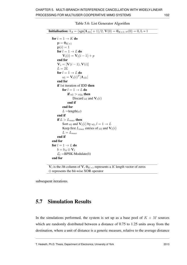
CHAPTER 5. MULTI-BRANCH INTERFERENCE CANCELLATION WITH WIDELY-LINEAR
PROCESSING FOR MULTIUSER COOPERATIVE MIMO SYSTEMS 102
Table 5.6: List Generator Algorithm
Initialisation: bA = (sgn[ΛA1] + 1)/2, V(0) = 0K×1, ω(0) = 0, L = 1
for i = 1→ K dop = 0K×1
p(i) = 1for l = 1→ L do
Vl(i) = Vl(i− 1) + pend forVi = [V(i− 1),V(i)]L = 2Lfor l = 1→ L do
ωl = Vl(i)T |ΛA1|
end forif 1st iteration of IDD then
for l = 1→ L doif ωl > ωth then
Discard ωl and Vl(i)end if
end forL =length(ω)
end ifif L > Lmax then
Sort ωl and Vl(i) by ωl, l = 1→ LKeep first Lmax entries of ωl and Vl(i)L = Lmax
end ifend forfor l = 1→ L do
b = bA ⊕Vl
Ll =BPSK-Modulate(b)end for
Vl is the lth column of V, 0K×1 represents a K length vector of zeros⊕ represents the bit-wise XOR operator
subsequent iterations.
5.7 Simulation Results
In the simulations performed, the system is set up as a base pool of K + M sources
which are randomly distributed between a distance of 0.75 to 1.25 units away from the
destination, where a unit of distance is a generic measure, relative to the average distance
T. Hesketh, Ph.D. Thesis, Department of Electronics, University of York 2013

CHAPTER 5. MULTI-BRANCH INTERFERENCE CANCELLATION WITH WIDELY-LINEAR
PROCESSING FOR MULTIUSER COOPERATIVE MIMO SYSTEMS 103
of 1 unit from the destination, which defines the base path loss in Eq.(5.7). For these
simulations, the base path loss at a distance of 1 unit is 20dB. From this pool, the M
closest sources to the destination are redefined as relays, to ensure the relays are well
positioned to transmit to the destination, with the rest of the source pool becoming the user
sources. The users distance from the newly defined relays (dsrm,k) is similarly modelled
as randomly distributed between a relative distance of 0.75 to 1.25 units.
0 5 10 15 20
10−5
10−4
10−3
10−2
10−1
100
SNR(dB)
BE
R
Non−Cooperative−WL−SIC
Non−Cooperative−MB−WL−SIC
Cooperative−Linear SIC
Cooperative−Linear MB−SIC
Cooperative−WL−SIC
Cooperative−MB−WL−SIC
Cooperative−Sphere Decoder
Figure 5.8: MIMO cooperative system with 2 AF relays, BPSK modulation, 8 singleantenna users, 2 antennas at destination
BPSK is the symbol modulation scheme used for the system, and the destination is
assumed to have 2 receive antennas. The channels are modelled with a LNS variance
of 6dB and a path-loss exponent of 4. To ensure a fair comparison of the cooperative
and non-cooperative cases, the Signal-to-Noise Ratio (SNR) axis is defined as the each
users source to destination SNR. The channels are also assumed to be quasi-static, and so
are unchanging over a packet, but non-correlated between packets, with the destination
having full knowledge of the system. Synchronous transmission by the relays in the
second phase of transmission is also assumed for simplicity although the system can be
generalized to asynchronous transmission. The non-cooperative case (where the relays
are not utilised) as well the cooperative case (where the relays are used) are considered in
T. Hesketh, Ph.D. Thesis, Department of Electronics, University of York 2013

CHAPTER 5. MULTI-BRANCH INTERFERENCE CANCELLATION WITH WIDELY-LINEAR
PROCESSING FOR MULTIUSER COOPERATIVE MIMO SYSTEMS 104
our results.
5 6 7 8 9 1010
−4
10−3
10−2
10−1
Number of Users
BE
R
Non−Cooperative−WL−SIC
Non−Cooperative−MB−WL−SIC
Cooperative−WL−SIC
Cooperative−MB−WL−SIC
Cooperative−Sphere Decoder
(a) 15dB SNR, BER vs K
0 5 10 15 2010
−5
10−4
10−3
10−2
10−1
SNR(dB)B
ER
Cooperative − MB WL SIC K = 6
Cooperative − MB WL SIC K = 7
Cooperative − MB WL SIC K = 8
Cooperative − MB WL SIC K = 9
Cooperative − MB WL SIC K = 10
Cooperative − MB WL SIC K = 11
Cooperative − MB WL SIC K = 12
(b) BER vs SNR
Figure 5.9: MIMO cooperative system with 2 AF relays and a variable number of singleantenna users, BPSK modulation, 2 antennas at destination
Fig. 5.8 shows the results for the non-cooperative and the cooperative case, with 4
branches being processed in the MB-WL-SIC for 8 user sources, with the system also
consisting of 2 AF relays. It can be seen that in the non-cooperative case, the WL-SIC
quickly reaches a high error floor, and although the MB-WL-SIC performs over 7dB
better, the MB-WL-SIC still reaches a relatively high error floor. For the cooperative
case, the MB-WL-SIC is shown to be comparable to the ML solution (produced using
the cooperative Sphere Decoder (SD) scheme in Chapter 3) up to a 15dB SNR, giving up
to 4dB of gain over the WL-SIC, with the MB-WL-SIC cooperative case showing up to
10dB of gain over the equivalent non-cooperative case. The WL SIC and WL MB SIC
can be seen to have over 7dB of gain each over the equivalent linear detectors for the
cooperative case, showing the advantage that WL filtering can give over linear filters for
BPSK.
Fig. 5.9(a) shows the BER as compared to the number of source users, for a system
with 2 AF relays with an SNR of 15dB, with a 2 antenna destination. It can be seen
that for up to 6-7 single antenna users, the cooperative MB-WL-SIC running 4 branches
is equivalent to the SD. For the non-cooperative schemes, the error rate has consistently
T. Hesketh, Ph.D. Thesis, Department of Electronics, University of York 2013

CHAPTER 5. MULTI-BRANCH INTERFERENCE CANCELLATION WITH WIDELY-LINEAR
PROCESSING FOR MULTIUSER COOPERATIVE MIMO SYSTEMS 105
at least an order of magnitude worse performance than the cooperative case. The gap
between the SD and MB-WL-SIC can be seen to widen as the number of users increases,
but the MB-WL-SIC still maintains roughly half a magnitude performance gain over the
WL-SIC. Fig. 5.9(b) shows the BER against the SNR for a varying number of users in
the same system, showing that above 7-8 users, the performance degrades by 2-3dB for
every extra user added.
1 2 3 4 5 610
−5
10−4
10−3
10−2
10−1
Number of Relays
BE
R
Non−Cooperative − WL−SIC
Non−Cooperative − MB−WL−SIC
Cooperative − WL−SIC
Cooperative − MB−WL−SIC
Cooperative − Sphere Decoder
Figure 5.10: MIMO cooperative system with a variable number of AF relays, BPSKmodulation, 8 single antenna users, 15dB SNR, 2 antennas at destination
Fig. 5.10 shows the BER as compared with the number of AF relays in the system for
8 users sources at 15dB SNR. As the number of relays increases, it can be seen that all
the proposed cooperative schemes reach an error floor at around 5-6 relays. This could be
due to the fact that the self interference between the relays becomes a major factor, and
results in diminishing gain returns as the number of relays increases. The non-cooperative
cases do not use the relays, and so remain at a constant performance level throughout.
Fig. 5.11 shows the BER performance against the SNR value for the dynamic branch
choice selection scheme, demonstrating how the BER performance changes as the shad-
T. Hesketh, Ph.D. Thesis, Department of Electronics, University of York 2013

CHAPTER 5. MULTI-BRANCH INTERFERENCE CANCELLATION WITH WIDELY-LINEAR
PROCESSING FOR MULTIUSER COOPERATIVE MIMO SYSTEMS 106
10 12 14 16 18 2010
−4
10−3
10−2
SNR(dB)
BE
R
MB−WL−SIC − 0.05 S
MB−WL−SIC − 0.1 S
MB−WL−SIC − 0.15 S
MB−WL−SIC − 0.2 S
MB−WL−SIC − 0.25 S
Figure 5.11: MIMO cooperative system with 2 AF relays, BPSK modulation, 8 singleantenna users, 2 antennas at destination, dynamic branch selection with a variable shad-owing criterion
owing criterion value S used for the dynamic branching scheme is altered. It can be seen
that for each 0.05 increment of S, the BER performance has between 0.5-1dB of gain at
high SNR values. It should also be noted, that if S is increased too high, that symbol es-
timates will begin to be described as unreliable erroneously, and start giving performance
loss, similar to the effect observed in Chapter 4 for the MF-SIC and MF-RO-SIC.
Fig. 5.12 shows the coded BER performance against the SNR value for the list-based
IDD system with an implementation of the WL, WL-SIC, and the proposed MB-WL-SIC
with 4 branches as in Section 5.6. For a fair comparison, the maximum list size Lmax
is set to B = 4. A rate 1/2 [7, 5] convolutional code with a memory of 2 is used by
the encoder and decoder in the IDD system, and it can be seen that for the first iteration,
the MB-WL-SIC has a 1.5dB performance gain over the WL-SIC, and up to 4dB of gain
over the WL filtering technique. For the third iteration, the MB-WL-SIC gains up to 2dB
from the first iteration, and about 1dB over the third iteration of the WL-SIC, with up
to 3.5dB of gain over the third iteration of the WL filter. It should be noted that at low
T. Hesketh, Ph.D. Thesis, Department of Electronics, University of York 2013

CHAPTER 5. MULTI-BRANCH INTERFERENCE CANCELLATION WITH WIDELY-LINEAR
PROCESSING FOR MULTIUSER COOPERATIVE MIMO SYSTEMS 107
0 1 2 3 4 5 6 7 8 9 10
10−4
10−3
10−2
10−1
SNR(dB)
Coded B
ER
Cooperative − WL− Iteration:1
Cooperative − WL−SIC − Iteration:1
Cooperative − MB−WL−SIC − Iteration:1
Cooperative − WL − Iteration:3
Cooperative − WL−SIC − Iteration:3
Cooperative − MB−WL−SIC − Iteration:3
Figure 5.12: Coded MIMO cooperative system with 2 AF relays, BPSK modulation, 8single antenna users, 2 antennas at destination
SNR values, the MB-WL-SIC does not offer any gain over the WL-SIC, and can give a
slight loss, suggesting that at very low SNR values, it is preferable to use the WL-SIC for
IDD. However, both the WL-SIC and MB-WL-SIC both give gains over the WL filtering
technique at low SNR values.
5.8 Summary
In this chapter, we have proposed a widely linear detection scheme for real-valued mod-
ulation schemes in an overloaded multi-user scenario with cooperative MIMO relaying,
with a proposed list IDD system based on the MB-WL-SIC detector. A method of dy-
namically selecting the branches of the MB-WL-SIC has been proposed, and a complex-
ity analysis of the proposed detector has been demonstrated. The proposed MB-WL-SIC
detection scheme has shown up to 4dB gains over the conventional WL-SIC in the coop-
T. Hesketh, Ph.D. Thesis, Department of Electronics, University of York 2013
CHAPTER 5. MULTI-BRANCH INTERFERENCE CANCELLATION WITH WIDELY-LINEAR
PROCESSING FOR MULTIUSER COOPERATIVE MIMO SYSTEMS 108
erative case, showing equivalent performance to the ML solution in some scenarios, with
also the WL techniques being seen to have over 7dB of gain over the equivalent linear
detectors for the cooperative case. The list-based IDD system has shown that the MB-
WL-SIC can give some gains over the WL-SIC, with subsequent iterations giving up to
2dB of extra gains, also demonstrating how the list-based algorithm can be applied to the
WL filtering and WL-SIC methods. It has been seen that the inclusion of a small number
of single antenna AF relays can boost the performance of the system significantly, and
give a low rate of errors in conjunction with the MB-WL-SIC, even in a very heavily
overloaded system. The DMB-WL-SIC has shown that MB performance gains can be
obtained, but with a lower average complexity cost, especially at high SNR values.
T. Hesketh, Ph.D. Thesis, Department of Electronics, University of York 2013

Chapter 6
Conclusions and Future Work
Contents6.1 Summary and Conclusions . . . . . . . . . . . . . . . . . . . . . . . 109
6.2 Future Work . . . . . . . . . . . . . . . . . . . . . . . . . . . . . . . 111
6.1 Summary and Conclusions
In this thesis, techniques of detection and link selection have been investigated and pro-
posed for MIMO and cooperative relay systems, with analyses of computational complex-
ity and implementations for IDD systems described. Results of simulation modelling for
the proposed techniques have been presented and discussed, showing primarily the BER
gains of the algorithms for a range of SNR values. Other metrics and parameters have
also been highlighted appropriately to the algorithms being presented.
In Chapter 3, a cross-layer design for a cooperative MIMO relay system is proposed,
deriving a cooperative ML detector for use with a SD from both phases of transmission
in the system, and using a summed channel approximation to take advantage of the sys-
tem information available at the destination device. The system model takes into account
distance and shadowing effects in the channel, as well as relay positioning. The proposed
cooperative ML detector is also formed such that the resulting channel that the SD oper-
ates on is the same matrix size as a non-cooperative, such that the SD will have a lower
T. Hesketh, Ph.D. Thesis, Department of Electronics, University of York
109
2013

CHAPTER 6. CONCLUSIONS AND FUTURE WORK 110
complexity for each time instant than the alternative of stacking the received signals.
For this system, two new combinatorial link selection schemes were proposed, extend-
ing previously proposed link selection schemes to take into account sets of relays in the
link selection metrics, rather than the individual relays. The proposed cooperative detec-
tor and link selection techniques were then integrated into an IDD system, which uses
the LSD and MAP detection techniques with convolutional channel coding. Simulation
results showed that the cooperative ML detector gives a good BER performance in the co-
operative MIMO system with distance shadowing fading effects, and compared this with
how the cooperative ML detector performs in system model from previous literature. The
proposed combinatorial link selection techniques were shown to give good gains in BER
performance over previous link selection strategies, but were also shown to have an in-
creased computational complexity cost as a trade-off. The IDD scheme was demonstrated
to work well with the proposed combinatorial link selection techniques for a rate 1/2 and
rate 1/3 convolutional channel code, giving up to a decade and half of BER gain over the
uncoded system.
In Chapter 4, a dynamically ordering, alternative cancellation candidate SIC detector
is proposed for a MIMO system, using the methods of RO, which is derived from the
LLR of the estimated data symbols, and the technique of MF, which tests for unreliable
data symbol estimates during the cancellation process using a shadow criterion area based
upon the Voronoi boundaries of the modulation scheme’s constellation diagram. RO and
MF techniques are combined into a single proposed detector, which is developed to reduce
the extra complexity required to process per time instant as compared with either RO or
MF, and a complexity analysis to compare the algorithms shows that the proposed MF-
RO-SIC requires very little extra complexity as compared to the RO-SIC. A hard decision
feedback IDD scheme is also developed, which uses the MAP detector, and re-encodes
the detected bits into estimated symbols that can be used in the SIC process to increase the
accuracy of the cancelled symbols in the next iteration of detection. Simulation results
showed that the proposed detector offers BER gains at high SNR values for both 4x4
and 8x8 systems, as well as for QPSK and 16-QAM modulation schemes. The effect on
performance of varying the shadow criterion and the number of alternative candidates is
shown, and the coded BER performance of the hard decision feedback IDD system with
the proposed MF-RO-SIC is shown to have gains over the IDD system with the RO-SIC
and MF-SIC.
T. Hesketh, Ph.D. Thesis, Department of Electronics, University of York 2013

CHAPTER 6. CONCLUSIONS AND FUTURE WORK 111
In Chapter 5, a WL based detector is proposed using the method of MB for a heav-
ily overloaded multiple user BPSK cooperative MIMO system. The WL-SIC is detailed
for the non-circular signal case, and the MB technique is discussed, with the two tech-
niques being combined, showing how the ordering of the branches involved is applied to
the system. The choice of MB branches is then investigated, with a method of dynami-
cally choosing branches during the cancellation process being developed, based upon the
shadow criterion used in MF techniques. The algorithm for hopping between different
branches is detailed, and a computational complexity analysis is performed, comparing
the different cancellation algorithms. A list-based IDD scheme is then developed, adapt-
ing the proposed MB-WL-SIC to give a list output, and a list generation algorithm is
detailed which is used to produce candidate lists from the single vector output of the WL
filter and WL-SIC, and also to generate new lists per iteration using the a priori LLRVs.
Simulation results show that the MB-WL-SIC can approach the cooperative ML detector
BER performance for the heavily overloaded multiple user cooperative system with the
use of a small number of AF relays. The BER performance of the proposed detector is also
investigated as the number of users and relays in the system changes. The performance of
the DMB-WL-SIC is also demonstrated for different values of the shadow criterion, and
the list-based IDD scheme is shown to have BER gains when using the proposed detector
with a list output.
6.2 Future Work
Many of the methods and algorithms detailed in this thesis have potential to be applied
to scenarios, systems and techniques outside the scope of this thesis, and there is further
work and analysis that could be considered to extend the work that has been covered.
Cooperative MIMO systems in this thesis are limited to just two phases of transmission
over a single set of relays, but this scenario could be extended to include multiple hops
and phases of transmission within the system, and as such each technique designed for
cooperative systems in this thesis could potentially be adapted for such a system. Of
particular application might be the combinatorial link selection algorithms proposed in
Chapter 3, and by extension the cross-layer cooperative ML detector design. Also, the
T. Hesketh, Ph.D. Thesis, Department of Electronics, University of York 2013

CHAPTER 6. CONCLUSIONS AND FUTURE WORK 112
overloaded multiple user cooperative system and the proposed methods in Chapter 5 could
find use in mobile communications or wireless sensor networks (WSN), as typically a
WSN consists of many small, single antenna devices transmitting at low data rates, that
can relay data between each device to a single destination in a mesh network, and this
fits well with the idea of using a few devices for simple relays, and the use of BPSK or
similar non-circular modulation schemes. Thus, the MB and WL techniques in Chapter 5
could be used in order to improve the accuracy of data reception in such a network.
The techniques of MF and RO can also be applied to most SIC based algorithms, and
it is possible to combine MF, RO, WL and MB methods together in many combinations,
which could be altered and tuned to suit the application or scenario in which the hybrid
detector would be used, with a great deal of flexibility due to the shadowing and candi-
date limit parameters of MF and the number and choice of branches in MB. The dynamic
branching algorithm in Chapter 5 can also be used for linear filter MB-SIC for circu-
lar signal systems, and could potentially be adapted for other interference cancellation
methods.
The three IDD schemes detailed during this thesis are generally portable to be used
with other types and sizes of channel coding schemes, as well as being applicable to a
variety of different detector algorithms. The LSD IDD scheme from Chapter 3 provides
a platform for any ML based detectors, the hard decision feedback method in Chapter
4 could be adapted to other interference cancellation methods reliant on cancelling esti-
mated symbols, and the list-based IDD method with the list generator in Chapter 5 can
be used with any detector that outputs a list or a single vector estimate of the transmitted
data, so there is a large scope of application.
T. Hesketh, Ph.D. Thesis, Department of Electronics, University of York 2013

Appendix
Derivation of Cooperative ML rule
Equating Eq. (3.15) and Eq. (3.16) gives:
‖ye − HeAex‖2 = ‖ysd − HsdAsx‖2 +∑mεΩs
‖yrdm − HrdmArmxm‖2 (A.1)
Using the matrix S defined in Eq. (3.19), we can find the approximation of the equated
ML rules to be:
‖ye − HeAex‖2 = ‖ysd − HsdAsx‖2 + ‖yrd − Sx‖2 (A.2)
Expanding these equations gives:
yHe ye + xH(HeAe)H(HeAe)x− yHe (HeAe)x− xH(HeAe)
Hye = yHs ys + yHrdyrd+
xH(AHs HH
s HsAs + SHS)x− (yHs HsAs + yHrdS)x− xH(AHs HH
s ys + SHyrd)
(A.3)
By equivalence, we can make the associations:
xH(HeAe)H(HeAe)x = xH(AH
s HHs HsAs + SHS)x (A.4)
xH(HeAe)Hye = xH(AH
s HHs ys + SHyrd) (A.5)
T. Hesketh, Ph.D. Thesis, Department of Electronics, University of York
113
2013

CHAPTER 6. CONCLUSIONS AND FUTURE WORK 114
Starting with Eq. (A.4) it is clear that:
(HeAe)H(HeAe) = (AH
s HHs HsAs + SHS) (A.6)
HeAe = (AHs HH
s HsAs + SHS)1/2 (A.7)
We can prove that the use of the matrix square root in this case is appropriate, as
AHs HH
s HsAs and SHS are clearly square positive definite Hermitian (SPDH) matrices,
and so their sum is also a SPDH.
Taking a SPDH matrix K of size n, we can diagonalise as such:
K = PHdiag(λ1, . . . , λn)P, (A.8)
where P is a unitary matrix, and λ is a positive eigenvalue. The matrix square root of K
is therefore:√
K = PHdiag(√λ1, . . . ,
√λn)P, (A.9)
which is clearly still a SPDH matrix. Therefore HeAe is also a SPDH, which therefore
means that HeAe = (HeAe)H , so (HeAe)
H(HeAe) = (HeAe)2 demonstrating that the
matrix square root is an appropriate operation in this case.
Using the result of Eq. (A.7) in Eq. (A.5) and rearranging gives:
ye = (HeAe)−1(AH
s HHs ys + SHyrd) (A.10)
T. Hesketh, Ph.D. Thesis, Department of Electronics, University of York 2013

Glossary
16-QAM 16 - Quadrature Amplitude Modulation
8-PSK 8 - Phase Shift Keying
AF Amplify and Forward
ARQ Automatic Repeat Request
ASK Amplitude Shift Keying
AWGN Additive White Gaussian Noise
BPSK Binary Phase Shift Keying
BER Bit Error Rate
CF Compress and Forward
CP Channel Power
CSI Channel State Information
DF Decode and Forward
DMB Dynamic Multiple Branch
ECC Error Correction Code
FEC Forward Error Correction
IDD Iterative Detection and Decoding
LDPC Low Density Parity Check
LLR Log Likelihood Ratio
LLRV Log Likelihood Ratio Value
LMS Least Mean Squares
LNS Log-Normal Shadowing
LOS Line-Of-Sight
LS Least Squares
LSD List Sphere Decoder
T. Hesketh, Ph.D. Thesis, Department of Electronics, University of York
115
2013

CHAPTER 6. CONCLUSIONS AND FUTURE WORK 116
MAP Maximum A Posteriori
MB Multiple Branch
MF Multiple Feedback
MH Maximum Harmonic
MHC Maximum Harmonic Combinatorial
MIMO Multiple-Input Multiple-Output
ML Maximum Likelihood
MM Maximum Minimum
MMC Maximum Minimum Combinatorial
MMSE Minimum Mean Square Error
MS Maximum Sum
MSE Mean Square Error
OSIC Ordered Successive Interference Cancellation
QPSK Quadrature Phase Shift Keying
RO Reliability Ordering
SD Sphere Decoder
SG Stochastic Gradient
SIC Successive Interference Cancellation
SINR Signal to Interference-plus-Noise Ratio
SISO Soft-Input Soft-Output
SNR Signal to Noise Ratio
SPDH Semi-Positive Definite Hermitian
VBLAST Vertical Bell LAbs Space-Time
WL Widely Linear
ZF Zero Forcing
T. Hesketh, Ph.D. Thesis, Department of Electronics, University of York 2013

Bibliography
[1] G. L. Turin, “Introduction to spread-spectrum antimultipath techniques and their
application to urban digital radio,” Proceedings of the IEEE, vol. 68, no. 3,
p. 328–353, 1980.
[2] H. Suzuki, “A Statistical Model for Urban Radio Propogation,” IEEE Transactions
on Communications, vol. 25, no. 7, p. 673–680, 1977.
[3] A. J. Rustako, N. Amitay, G. J. Owens and R. S. Roman, “Radio propagation at
microwave frequencies for line-of-sight microcellular mobile and personal commu-
nications,” IEEE Transactions on Vehicular Technology, vol. 40, no. 1, p. 203–210,
1991.
[4] R. C. Lee, M. Chiu, and J. Lin, Communications engineering essentials for com-
puter scientists and electrical engineers. Singapore; Hoboken, NJ: IEEE Press :
John Wiley & Sons (Asia), 2007.
[5] A. F. Molisch, Wireless communications. Chichester, West Sussex, U.K.: Wiley :
IEEE, 2011.
[6] M. Shafi, S. Ogose, and T. Hattori, Wireless communications in the 21st century.
Piscataway, NJ; [New York]: IEEE Press ; Wiley-Interscience, 2002.
[7] Y. Cho, J. Kim, W. Yang, and C. Kang, MIMO-OFDM wireless communications
with MATLAB. Singapore ;;Hoboken NJ: IEEE Press ;J. Wiley & Sons (Asia),
2010.
[8] H. Bolcskei, “MIMO-OFDM wireless systems: basics, perspectives, and chal-
lenges,” Wireless Communications, IEEE, vol. 13, no. 4, p. 31–37, 2006.
T. Hesketh, Ph.D. Thesis, Department of Electronics, University of York
117
2013

BIBLIOGRAPHY 118
[9] G. Golden, C. Foschini, R. Valenzuela, and P. Wolniansky, “Detection algorithm
and initial laboratory results using V-BLAST space-time communication architec-
ture,” Electronics Letters, vol. 35, no. 1, p. 14, 1999.
[10] N. Kim, Y. Lee, and H. Park, “Performance analysis of MIMO system with linear
MMSE receiver,” IEEE Transactions on Wireless Communications, vol. 7, no. 11,
pp. 4474–4478, Nov. 2008.
[11] G. Foschini and M. Gans, “On limits of wireless communications in a fading envi-
ronment when using multiple antennas,” Wireless personal communications, vol. 6,
no. 3, p. 311–335, 1998.
[12] E. Telatar, “Capacity of multi-antenna gaussian channels,” European Transactions
on Telecommunications, vol. 10, no. 6, pp. 585–595, Nov. 1999.
[13] S. Alamouti, “A simple transmit diversity technique for wireless communications,”
IEEE Journal on Selected Areas in Communications, vol. 16, no. 8, pp. 1451–1458,
Oct. 1998.
[14] M. Dohler and Y. Li, Cooperative communications : hardware, channel & PHY.
Chichester West Sussex U.K. Hoboken NJ: Wiley, 2010.
[15] D. Chen and J. N. Laneman, “Modulation and demodulation for cooperative diver-
sity in wireless systems,” Wireless Communications, IEEE Transactions on, vol. 5,
no. 7, p. 1785–1794, 2006.
[16] A. Nosratinia, T. E. Hunter, and A. Hedayat, “Cooperative communication in wire-
less networks,” Communications Magazine, IEEE, vol. 42, no. 10, p. 74–80, 2004.
[17] A. Sadek, W. Su, and K. Liu, “Multinode cooperative communications in wireless
networks,” IEEE Transactions on Signal Processing, vol. 55, no. 1, pp. 341–355,
Jan. 2007.
[18] A. Sendonaris, E. Erkip, and B. Aazhang, “User cooperation diversity-part II: im-
plementation aspects and performance analysis,” IEEE Transactions on Communi-
cations, vol. 51, no. 11, pp. 1939–1948, Nov. 2003.
[19] J. Laneman, D. Tse, and G. Wornell, “Cooperative diversity in wireless networks:
Efficient protocols and outage behavior,” IEEE Transactions on Information The-
ory, vol. 50, no. 12, pp. 3062–3080, Dec. 2004.
T. Hesketh, Ph.D. Thesis, Department of Electronics, University of York 2013

BIBLIOGRAPHY 119
[20] P. Clarke and R. C. de Lamare, “Transmit diversity and relay selection algorithms
for multirelay cooperative MIMO systems,” IEEE Transactions on Vehicular Tech-
nology, vol. 61, no. 3, pp. 1084–1098, Mar. 2012.
[21] S. Yang and J. Belfiore, “Optimal Space-Time codes for the MIMO Amplify-and-
Forward cooperative channel,” IEEE Transactions on Information Theory, vol. 53,
no. 2, pp. 647–663, Feb. 2007.
[22] W. J. Huang, Y. W. Hong, and C. C. Kuo, “Decode-and-forward cooperative re-
lay with multi-user detection in uplink CDMA networks,” in Proc. IEEE Global
Telecommunications Conference, 2007, p. 4397–4401.
[23] J. Luo, R. S. Blum, L. J. Cimini, L. J. Greenstein, and A. M. Haimovich, “Decode-
and-forward cooperative diversity with power allocation in wireless networks,”
Wireless Communications, IEEE Transactions on, vol. 6, no. 3, p. 793–799, 2007.
[24] T. Rappaport, Wireless communications : principles and practice, 2nd ed. Upper
Saddle River N.J.: Prentice Hall PTR, 2002.
[25] H. Zhang, J. Wang, T. Lu, and T. A. Gulliver, “Capacity of 60 GHz wireless com-
munication systems over ricean fading channels.” IEEE, Aug. 2011, pp. 437–440.
[26] G. Li and K. Yu, “Modelling and simulation of coherent weibull clutter,” IEE Pro-
ceedings, Part F: Radar and Signal Processing, vol. 136, no. 1, pp. 2–12, Feb.
1989.
[27] N. S. Adawi, H. L. Bertoni, J. R. Child, W. A. Daniel, J. E. Dettra, and R. P.
Eckert, “Coverage prediction for mobile radio systems operating in the 800/900
MHz frequency range,” IEEE Transactions on Vehicular Technology, vol. 37, no. 1,
pp. 3–72, Feb. 1988.
[28] H. Hashemi, “The indoor radio propagation channel,” Proceedings of the IEEE,
vol. 81, no. 7, pp. 943–968, Jul. 1993.
[29] Q. Zhu, X. Yu, J. Wang, D. Xu, and X. Chen, “A new generation method for Spatial-
Temporal correlated MIMO nakagami fading channel,” International Journal of
Antennas and Propagation, vol. 2012, pp. 1–8, 2012.
[30] H. Hsu, Schaum’s outline of theory and problems of probability, random variables,
and random processes. New York: McGraw-Hill, 1997.
T. Hesketh, Ph.D. Thesis, Department of Electronics, University of York 2013

BIBLIOGRAPHY 120
[31] V. Erceg, L. Greenstein, S. Tjandra, S. Parkoff, A. Gupta, B. Kulic, A. Julius, and
R. Bianchi, “An empirically based path loss model for wireless channels in subur-
ban environments,” IEEE Journal on Selected Areas in Communications, vol. 17,
no. 7, pp. 1205–1211, Jul. 1999.
[32] A. Paulraj and C. Papadias, “Space-time processing for wireless communications,”
IEEE Signal Processing Magazine, vol. 14, no. 6, pp. 49–83, Nov. 1997.
[33] J. Barnes and D. Allan, “A statistical model of flicker noise,” Proceedings of the
IEEE, vol. 54, no. 2, pp. 176–178, 1966.
[34] T. Sreenivas and P. Kirnapure, “Codebook constrained wiener filtering for speech
enhancement,” IEEE Transactions on Speech and Audio Processing, vol. 4, no. 5,
pp. 383–389, Sep. 1996.
[35] L. Liu and T. Shimamura, “Pink noise whitening method for pitch synchronous
LPC analysis,” in Signal & Information Processing Association Annual Summit
and Conference (APSIPA ASC), 2012 Asia-Pacific, Hollywood, CA, Dec. 2012,
pp. 1–6.
[36] C. Studer, “Iterative MIMO decoding: Algorithms and VLSI implementation as-
pects,” Ph.D. dissertation, ETH Zurich, Zurich, 2009.
[37] A. Stefanov and E. Erkip, “Cooperative Space-Time coding for wireless networks,”
IEEE Transactions on Communications, vol. 53, no. 11, pp. 1804–1809, Nov. 2005.
[38] N. Kim and H. Park, “Bit error performance of convolutional coded MIMO sys-
tem with linear MMSE receiver,” IEEE Transactions on Wireless Communications,
vol. 8, no. 7, pp. 3420–3424, Jul. 2009.
[39] A. Berthet, B. Unal, and R. Visoz, “Iterative decoding of convolutionally encoded
signals over multipath rayleigh fading channels,” IEEE Journal on Selected Areas
in Communications, vol. 19, no. 9, pp. 1729–1743, Sep. 2001.
[40] J. Heller and I. Jacobs, “Viterbi decoding for satellite and space communication,”
IEEE Transactions on Communications, vol. 19, no. 5, pp. 835–848, Oct. 1971.
[41] J. Omura, “On the viterbi decoding algorithm,” IEEE Transactions on Information
Theory, vol. 15, no. 1, pp. 177–179, Jan. 1969.
T. Hesketh, Ph.D. Thesis, Department of Electronics, University of York 2013

BIBLIOGRAPHY 121
[42] R. McEliece, “On the BCJR trellis for linear block codes,” IEEE Transactions on
Information Theory, vol. 42, no. 4, pp. 1072–1092, Jul. 1996.
[43] C. Berrou and A. Glavieux, “Near optimum error correcting coding and decoding:
turbo-codes,” IEEE Transactions on Communications, vol. 44, no. 10, pp. 1261–
1271, Oct. 1996.
[44] J. Hagenauer, E. Offer and L. Papke, “Iterative decoding of binary block and con-
volutional codes,” IEEE Transactions on Information Theory, vol. 42, no. 2, pp.
429–445, Mar. 1996.
[45] T. J. Richardson, M. A. Shokrollahi and R. L. Urbanke, “Design of capacity-
approaching irregular low-density parity-check codes,” IEEE Transactions on In-
formation Theory, vol. 47, no. 2, pp. 619–637, Feb. 2001.
[46] V. Oksman, and S. Galli, “G.hn: The new ITU-T home networking standard,” IEEE
Communications Magazine, vol. 47, no. 10, pp. 138–145, Oct. 2009.
[47] B. Classon, K. Blankenship, and V. Desai, “Channel coding for 4G systems with
adaptive modulation and coding,” IEEE Wireless Communications, vol. 9, no. 2,
pp. 8–13, Apr. 2002.
[48] S. Haykin, Adaptive filter theory., 4th ed. Upper Saddle River N.J.: Prentice Hall,
2002.
[49] T. Wang, R. C. de Lamare and P. Mitchell, “Low-Complexity Set-Membership
Channel Estimation for Cooperative Wireless Sensor Networks,” IEEE Transac-
tions on Vehicular Technology, vol. 60, no. 6, pp. 2594–2607, Jul. 2011.
[50] T. Wang, R. C. de Lamare and P. Mitchell, “Low-Complexity Channel Estimation
for Cooperative Wireless Sensor Networks Based on Data Selection,” in Vehicular
Technology Conference (VTC 2010-Spring), Taipei, Taiwan, May. 2010, pp. 1–5.
[51] E. Karami, “Tracking performance of least squares MIMO channel estimation al-
gorithm,” IEEE Transactions on Communications, vol. 55, no. 11, pp. 2201–2209,
Nov. 2007.
[52] Y. Eldar and A. Oppenheim, “Covariance shaping least-squares estimation,” IEEE
Transactions on Signal Processing, vol. 51, no. 3, pp. 686–697, Mar. 2003.
T. Hesketh, Ph.D. Thesis, Department of Electronics, University of York 2013

BIBLIOGRAPHY 122
[53] L. E. Pooh, W. G. Lim, and H. Ali, “Adaptive channel estimation using least mean
squares algorithm for cyclic prefix OFDM systems,” in 2009 IEEE 9th Malaysia
International Conference on Communications (MICC), Kuala Lumpur, Malaysia,
Dec. 2009, pp. 789–793.
[54] S. Kinjo, “A new MMSE channel estimation algorithm for OFDM systems,” IEICE
Electronics Express, vol. 5, no. 18, pp. 738–743, 2008.
[55] M. Biguesh and A. Gershman, “Training-based MIMO channel estimation: a study
of estimator tradeoffs and optimal training signals,” IEEE Transactions on Signal
Processing, vol. 54, no. 3, pp. 884–893, Mar. 2006.
[56] R. Trepkowski, “Channel estimation strategies for coded MIMO systems,” Ph.D.
dissertation, Virginia Polytechnic Institute and State University, 2004.
[57] R. C. de Lamare, “Joint iterative power allocation and linear interference sup-
pression algorithms for cooperative DS-CDMA networks,” IET Communications,
vol. 6, no. 13, pp.1930–1942, Sep. 2012.
[58] T. Wang, R. C. de Lamare and A. Schmeink, “Joint Linear Receiver Design and
Power Allocation Using Alternating Optimization Algorithms for Wireless Sensor
Networks,” IEEE Transactions on Vehicular Technology, vol. 61, no. 9, pp.4129–
4141, Nov. 2012.
[59] Z. Yi, R. Adve, and J. L. Teng, “Improving amplify-and-forward relay networks:
optimal power allocation versus selection,” IEEE Transactions on Wireless Com-
munications, vol. 6, no. 8, pp.3114–3123, Aug. 2007.
[60] P. Clarke and R. C. de Lamare, “Joint transmit diversity optimization and relay
selection for Multi-Relay cooperative MIMO systems using discrete stochastic al-
gorithms,” IEEE Communications Letters, vol. 15, no. 10, pp. 1035–1037, 2011.
[61] A. Klein, G. Kaleh, and P. Baier, “Zero forcing and minimum mean-square-error
equalization for multiuser detection in code-division multiple-access channels,”
IEEE Transactions on Vehicular Technology, vol. 45, no. 2, pp. 276–287, May
1996.
T. Hesketh, Ph.D. Thesis, Department of Electronics, University of York 2013

BIBLIOGRAPHY 123
[62] R. H. Y. Louie, Y. Li, and B. Vucetic, “Zero forcing in general Two-Hop relay
networks,” IEEE Transactions on Vehicular Technology, vol. 59, no. 1, pp. 191–
202, Jan. 2010.
[63] H. Poor and S. Verdu, “Probability of error in MMSE multiuser detection,” IEEE
Transactions on Information Theory, vol. 43, no. 3, pp. 858–871, May 1997.
[64] B. Picinbono and P. Chevalier, “Widely linear estimation with complex data,” IEEE
Transactions on Signal Processing, vol. 43, no. 8, pp. 2030–2033, Aug. 1995.
[65] F. Sterle, “Widely linear MMSE transceivers for MIMO channels,” IEEE Transac-
tions on Signal Processing, vol. 55, no. 8, pp. 4258–4270, Aug. 2007.
[66] G. Gelli, L. Paura, and A. Ragozini, “Blind widely linear multiuser detection,”
IEEE Communications Letters, vol. 4, no. 6, pp. 187–189, Jun. 2000.
[67] S. Buzzi, M. Lops, and S. Sardellitti, “Widely linear reception strategies for layered
space-time wireless communications,” IEEE Transactions on Signal Processing,
vol. 54, no. 6, pp. 2252–2262, Jun. 2006.
[68] T. Liu, “Some results for the fast MMSE-SIC detection in spatially multiplexed
MIMO systems,” IEEE Transactions on Wireless Communications, vol. 8, no. 11,
pp. 5443–5448, Nov. 2009.
[69] C. Ling, W. H. Mow, and L. Gan, “Dual-Lattice ordering and partial lattice reduc-
tion for SIC-Based MIMO detection,” IEEE Journal of Selected Topics in Signal
Processing, vol. 3, no. 6, pp. 975–985, Dec. 2009.
[70] M. Damen, H. E. Gamal, and G. Caire, “On maximum-likelihood detection and
the search for the closest lattice point,” IEEE Transactions on Information Theory,
vol. 49, no. 10, pp. 2389–2402, Oct. 2003.
[71] S. Verdu, “Minimum probability of error for asynchronous gaussian multiple-
access channels,” IEEE Transactions on Information Theory, vol. 32, no. 1, pp.
85–96, Jan. 1986.
[72] R. C. de Lamare and R. Sampaio-Neto, “Minimum Mean-Squared error iterative
successive parallel arbitrated decision feedback detectors for DS-CDMA systems,”
IEEE Transactions on Communications, vol. 56, no. 5, pp. 778–789, May 2008.
T. Hesketh, Ph.D. Thesis, Department of Electronics, University of York 2013
BIBLIOGRAPHY 124
[73] L. Yang, “Receiver multiuser diversity aided Multi-Stage MMSE multiuser detec-
tion for DS-CDMA and SDMA systems employing I-Q modulation,” in Vehicular
Technology Conference Fall (VTC 2010-Fall), 2010 IEEE 72nd. IEEE, Sep. 2010,
pp. 1–5.
[74] N. Song, R. C. de Lamare, M. Haardt, and M. Wolf, “Adaptive widely linear
Reduced-Rank interference suppression based on the multistage wiener filter,”
IEEE Transactions on Signal Processing, vol. 60, no. 8, pp. 4003–4016, Aug. 2012.
[75] J. Olivier and W. Kleynhans, “Single antenna interference cancellation for synchro-
nised GSM networks using a widely linear receiver,” IET Communications, vol. 1,
no. 1, p. 131, 2007.
[76] A. Aghaei, K. Plataniotis, and S. Pasupathy, “Widely linear MMSE receivers for
linear dispersion space-time block-codes,” IEEE Transactions on Wireless Com-
munications, vol. 9, no. 1, pp. 8–13, Jan. 2010.
[77] J. G. Andrews, “Interference cancellation for cellular systems: A contemporary
overview,” Wireless Communications, IEEE, vol. 12, no. 2, p. 19–29, 2005.
[78] J. Benesty, Y. Huang, and J. Chen, “A fast recursive algorithm for optimum sequen-
tial signal detection in a BLAST system,” IEEE Transactions on Signal Processing,
vol. 51, no. 7, pp. 1722–1730, Jul. 2003.
[79] Y. Shang and X. gen Xia, “On fast recursive algorithms for V-BLAST with optimal
ordered SIC detection,” IEEE Transactions on Wireless Communications, vol. 8,
no. 6, pp. 2860–2865, Jun. 2009.
[80] J. Choi, Heeju, and Y. Lee, “Adaptive MIMO decision feedback equalization for
receivers with time-varying channels,” IEEE Transactions on Signal Processing,
vol. 53, no. 11, pp. 4295–4303, Nov. 2005.
[81] G. J. Foschini, “Layered space-time architecture for wireless communication in
a fading environment when using multi-element antennas,” Bell Labs Technical
Journal, vol. 1, no. 2, pp. 41–59, 1996.
[82] C. Windpassinger, L. Lampe, R. Fischer, and T. Hehn, “A performance study of
MIMO detectors,” IEEE Transactions on Wireless Communications, vol. 5, no. 8,
pp. 2004–2008, Aug. 2006.
T. Hesketh, Ph.D. Thesis, Department of Electronics, University of York 2013

BIBLIOGRAPHY 125
[83] R. C. de Lamare, “Joint iterative power allocation and interference suppression
algorithms for cooperative spread spectrum networks,” in Acoustics Speech and
Signal Processing (ICASSP), 2010 IEEE International Conference on. IEEE,
2010, pp. 3178–3181.
[84] G. Kramer, M. Gastpar, and P. Gupta, “Cooperative strategies and capacity theo-
rems for relay networks,” IEEE Transactions on Information Theory, vol. 51, no. 9,
pp. 3037–3063, Sep. 2005.
[85] K. Amiri, M. Wu, J. R. Cavallaro, and J. Lilleberg, “Cooperative partial detection
using MIMO relays,” IEEE Transactions on Signal Processing, vol. 59, pp. 5039–
5049, Oct. 2011.
[86] K. Amiri, M. Wu, M. Duarte, and J. R. Cavallaro, “Physical layer algorithm and
hardware verification of MIMO relays using cooperative partial detection,” in 2010
IEEE International Conference on Acoustics, Speech and Signal Processing, Dal-
las, TX, USA, 2010, pp. 5614–5617.
[87] S. Han and C. Tellambura, “Complexity-efficient detection for MIMO relay net-
works,” in Information Theory (CWIT), 2011 12th Canadian Workshop on. IEEE,
May 2011, pp. 126–129.
[88] T. Hesketh, P. Clarke, R. C. de Lamare, and S. Wales, “Joint maximum likelihood
detection and power allocation in cooperative MIMO relay systems,” in Smart An-
tennas (WSA), 2012 International ITG Workshop on. IEEE, Mar. 2012, pp. 325–
331.
[89] Y. Fan and J. Thompson, “MIMO configurations for relay channels: Theory and
practice,” IEEE Transactions on Wireless Communications, vol. 6, no. 5, pp. 1774–
1786, May 2007.
[90] M. Zorzi, “Power control and diversity in mobile radio cellular systems in the pres-
ence of ricean fading and log-normal shadowing,” IEEE Transactions on Vehicular
Technology, vol. 45, no. 2, pp. 373–382, May 1996.
[91] A. Nasri and R. Schober, “Performance of cooperative diversity systems in Non-
Gaussian environments,” in Communications (ICC), 2010 IEEE International Con-
ference on. Cape Town: IEEE, May 2010, pp. 1–6.
T. Hesketh, Ph.D. Thesis, Department of Electronics, University of York 2013

BIBLIOGRAPHY 126
[92] I. Krikidis, J. Thompson, S. Mclaughlin, and N. Goertz, “Amplify-and-forward
with partial relay selection,” IEEE Communications Letters, vol. 12, no. 4, pp.
235–237, Apr. 2008.
[93] Y. Jing and H. Jafarkhani, “Single and multiple relay selection schemes and their
achievable diversity orders,” IEEE Transactions on Wireless Communications,
vol. 8, no. 3, pp. 1414–1423, Mar. 2009.
[94] D. S. Michalopoulos, H. A. Suraweera, G. K. Karagiannidis, and R. Schober,
“Amplify-and-Forward relay selection with outdated channel state information,” in
Global Telecommunications Conference (GLOBECOM 2010), 2010 IEEE. IEEE,
Dec. 2010, pp. 1–6.
[95] A. Ikhlef, D. S. Michalopoulos, and R. Schober, “Buffers improve the perfor-
mance of relay selection,” in Global Telecommunications Conference (GLOBE-
COM 2011), 2011 IEEE. IEEE, Dec. 2011, pp. 1–6.
[96] J. Yang, Z. Zhang, and W. Meng, “A novel relay selection scheme in multi-antenna
cooperative systems,” in Software Engineering and Service Sciences (ICSESS),
2010 IEEE International Conference on. IEEE, Jul. 2010, pp. 427–430.
[97] A. Bletsas, A. Khisti, D. Reed, and A. Lippman, “A simple cooperative diversity
method based on network path selection,” IEEE Journal on Selected Areas in Com-
munications, vol. 24, no. 3, pp. 659–672, Mar. 2006.
[98] H. Vikalo, B. Hassibi, and T. Kailath, “Iterative decoding for MIMO channels
via modified sphere decoding,” IEEE Transactions on Wireless Communications,
vol. 3, no. 6, pp. 2299–2311, Nov. 2004.
[99] X. Wang and H. Poor, “Iterative (turbo) soft interference cancellation and decoding
for coded CDMA,” IEEE Transactions on Communications, vol. 47, no. 7, pp.
1046–1061, Jul. 1999.
[100] H. Le, B. Lee, and I. Lee, “Iterative detection and decoding with an improved
V-BLAST for MIMO-OFDM systems,” IEEE Journal on Selected Areas in Com-
munications, vol. 24, no. 3, pp. 504–513, Mar. 2006.
[101] S. ten Brink and B. Hochwald, “Detection thresholds of iterative MIMO process-
ing.” IEEE, 2002, p. 22.
T. Hesketh, Ph.D. Thesis, Department of Electronics, University of York 2013

BIBLIOGRAPHY 127
[102] B. Hochwald and S. ten Brink, “Achieving near-capacity on a multiple-antenna
channel,” IEEE Transactions on Communications, vol. 51, no. 3, pp. 389–399,
Mar. 2003.
[103] P. W. Wolniansky, G. J. Foschini, G. D. Golden, and R. A. Valenzuela, “V-BLAST:
an architecture for realizing very high data rates over the rich-scattering wireless
channel,” in Signals, Systems, and Electronics, 1998. ISSSE 98. 1998 URSI Inter-
national Symposium on, 2002, p. 295–300.
[104] D, Wubben, R. Bohnke, V. Kuhn, and K. D. Kammeyer, “MMSE extension of V-
BLAST based on sorted QR decomposition,” in IEEE Vehicular Technology Con-
ference Fall (VTC 2003-Fall). IEEE, Oct. 2003, pp. 508–512.
[105] R. C. de Lamare,“Adaptive and Iterative Multi-Branch MMSE Decision Feedback
Detection Algorithms for Multi-Antenna Systems,” IEEE Transactions on Wireless
Communications, vol. 12, no. 10, pp.5294–5308, Oct. 2013.
[106] R. Fa and R. C. de Lamare, “Multi-branch successive interference cancellation for
MIMO spatial multiplexing systems: design, analysis and adaptive implementa-
tion,” IET Communications, vol. 5, no. 4, p. 484, 2011.
[107] P. Li, R. C. de Lamare, and R. Fa, “Multiple feedback successive interference can-
cellation detection for multiuser MIMO systems,” IEEE Transactions on Wireless
Communications, vol. 10, no. 8, pp. 2434–2439, Aug. 2011.
[108] Y. Cai and R. de Lamare, “Space-Time adaptive MMSE multiuser decision feed-
back detectors with Multiple-Feedback interference cancellation for CDMA sys-
tems,” IEEE Transactions on Vehicular Technology, vol. 58, no. 8, pp. 4129–4140,
Oct. 2009.
[109] P. Li and R. C. D. Lamare, “Adaptive Decision-Feedback detection with constella-
tion constraints for MIMO systems,” IEEE Transactions on Vehicular Technology,
vol. 61, no. 2, pp. 853–859, Feb. 2012.
[110] L. Yang, “Using Multi-Stage MMSE detection to approach optimum error perfor-
mance in multiantenna MIMO systems,” in Vehicular Technology Conference Fall
(VTC 2009-Fall), 2009 IEEE 70th. IEEE, Sep. 2009, pp. 1–5.
T. Hesketh, Ph.D. Thesis, Department of Electronics, University of York 2013

BIBLIOGRAPHY 128
[111] G. Voronoı, “Nouvelles applications des parametres continus a la theorie des
formes quadratiques. Deuxieme memoire. Recherches sur les parallelloedres prim-
itifs,” Journal fur die reine und angewandte Mathematik, vol. 134, pp. 198–287,
1908.
[112] A. Okabe, B. Boots, K. Sugihara, S. N. Chiu, Spatial tessellations: concepts and
applications of Voronoi diagrams. Chichester, West Sussex, U.K.: Wiley, 2009.
[113] F. Aurenhammer, “Voronoi diagrams - a survey of a fundamental geometric data
structure,” ACM Computing Surveys (CSUR), vol. 23, no. 3, pp. 345–405, 1991.
[114] X. Li, and J. A. Ritcey, “Bit-interleaved coded modulation with iterative decoding,”
in IEEE International Conference on Communications. IEEE, 1999, pp. 858–863.
[115] W. Gerstacker, R. Schober, and A. Lampe, “Receivers with widely linear pro-
cessing for frequency-selective channels,” IEEE Transactions on Communications,
vol. 51, no. 9, pp. 1512–1523, Sep. 2003.
[116] R. Schober, W. Gerstacker, and L. Lampe, “A widely linear DF-MMSE receiver for
DS-CDMA with BPSK modulation,” in Global Telecommunications Conference,
2003. GLOBECOM ’03. IEEE, 2003, pp. 1548–1552.
[117] S. Abdallah and I. N. Psaromiligkos, “Widely linear versus conventional Subspace-
Based estimation of SIMO Flat-Fading channels: Mean squared error analysis,”
IEEE Transactions on Signal Processing, vol. 60, no. 3, pp. 1307–1318, Mar. 2012.
[118] S. Verdu, Multiuser detection. Cambridge ; New York: Cambridge University
Press, 1998.
[119] P. Chevalier and F. Dupuy, ”Widely Linear Alamouti Receiver for the Recep-
tion of Real-Valued Constellations Corrupted by Interferences-The Alamouti-
SAIC/MAIC Concept,” IEEE Transactions on Signal Processing, vol. 59, no. 7,
pp. 3339–3354, Jul. 2011.
[120] A. Cacciapuoti, G. Gelli, L. Paura, and F. Verde, “Widely linear versus linear blind
multiuser detection with Subspace-Based channel estimation: Finite Sample-Size
effects,” IEEE Transactions on Signal Processing, vol. 57, no. 4, pp. 1426–1443,
Apr. 2009.
T. Hesketh, Ph.D. Thesis, Department of Electronics, University of York 2013
BIBLIOGRAPHY 129
[121] P. Li, R. C. de Lamare, and R. Fa, “Multi-Feedback successive interference can-
cellation with Multi-Branch processing for MIMO systems,” in VTC Spring 2011 -
IEEE 73rd Vehicular Technology Conference. IEEE, May 2011, pp. 1–5.
[122] R. C. de Lamare and D. L. Ruyet, “Multi-branch MMSE decision feedback detec-
tion algorithms with error propagation mitigation for MIMO systems,” in Interna-
tional Conference on Acoustics Speech and Signal Processing (ICASSP). IEEE,
Mar. 2010, pp. 3450–3453.
[123] S. Nammi, “Threshold list subset detector for turbo MIMO systems” in European
Wireless Conference (EW). IEEE, Mar. 2009, pp. 276–281.
[124] S. Nammi, and D. K. Borah, “Iterative List Subset Detectors for Turbo Product
Coded MIMO Wireless Systems.” in VTC Spring 2007 - IEEE Vehicular Technol-
ogy Conference. IEEE, Apr. 2007, pp. 2023–2027.
T. Hesketh, Ph.D. Thesis, Department of Electronics, University of York 2013