WP/08/228

Determinants of Government Efficiency

David Hauner and Annette Kyobe

© 2008 International Monetary Fund WP/08/228 IMF Working Paper Fiscal Affairs Department

Determinants of Government Efficiency

Prepared by David Hauner and Annette Kyobe1

Authorized for distribution by Steven A. Symansky

September 2008

Abstract

This Working Paper should not be reported as representing the views of the IMF. The views expressed in this Working Paper are those of the author(s) and do not necessarily represent those of the IMF or IMF policy. Working Papers describe research in progress by the author(s) and are published to elicit comments and to further debate.

We compile the first large cross-country panel dataset of public sector performance and efficiency, encompassing 114 countries on all income levels from 1980 to 2006, with about 1,800 country-year observations for the education sector and about 900 observations for health. We regress these indicators on potential economic, institutional, demographic, and geographic determinants. Our most resounding conclusion is that higher government expenditure relative to GDP tends to be associated with lower efficiency in the respective sector. Moreover, we find that richer countries exhibit better public sector performance and efficiency, and that institutional and demographic factors also play a significant role. JEL Classification Numbers: D50, D78 Keywords: Public sector performance; expenditure efficiency; fiscal policy; institutions. Author’s E-Mail Address: dhauner@imf.org; akyobe@imf.org 1 We are grateful to Marijn Verhoeven and Victoria Gunnarson for invaluable advice on methodology and data sources and to Mark De Broeck and Marijn Verhoeven for helpful comments.

2

Contents Page

I. Introduction ............................................................................................................................3

II. Methodology .........................................................................................................................5

III. Government Efficiency, 1980–2004....................................................................................8

IV. Determinants of Government Efficiency...........................................................................13 A. Economic Determinants..........................................................................................16 B. Institutional Determinants .......................................................................................17 C. Demographic and Geographic Determinants ..........................................................18

V. Conclusions.........................................................................................................................19

VI. Appendix............................................................................................................................20 A. Data Sources ...........................................................................................................20 B. Countries Included ..................................................................................................21 C. Background Tables..................................................................................................21

References................................................................................................................................24 Tables 1. Summary of Scores ..............................................................................................................10 2. Spearman Rank Order Correlations .....................................................................................10 3. Tested-Down Regressions ...................................................................................................14 4. Overview of Univariate and Tested-Down Regressions......................................................15 A1. Summary of Determinants ................................................................................................21 A2. Univariate Regressions .....................................................................................................22 A3. Multivariate Regressions...................................................................................................23 Figures 1. Plots of PSP, PSE, and DEA Scores in Education and Health ............................................11 2. Evolution of Health and Education Spending, Performance, and Efficiency in Advanced and Developing Economies ............................................................................................................12

3

I. INTRODUCTION

The efficiency of government spending has become one of the key issues in public finance. In the advanced economies and many transition countries, higher efficiency of spending seems to be the only way to avoid that public services are squeezed out between the opposing forces of age-related expenditure and rising tax competition (Heller and Hauner, 2006). In low-income countries, increased expenditure efficiency will have to complement increased social expenditure if the Millennium Development Goals are to be reached. Emerging markets, in turn, may seem under less pressure of this kind, given their rapid growth, but it is well-known that the demand for public services tends to rapidly increase as countries become richer (the so-called Wagner effect), and higher efficiency will be the only way to avoid a large increase in the tax burden. Moreover, good government is also of more general concern, as it has been shown, for example by Easterly and Levine (1997), that it is a crucial determinant of economic growth.

Against this background, government efficiency at the aggregate level has thus become the subject of a rapidly growing literature, including key contributions by Gupta and Verhoeven (2001), Tanzi and Schuknecht (1997, 2000), and Afonso et al. (2005). These studies typically measure public sector efficiency by relating government expenditure to socio-economic indicators that are assumed to be targeted by public spending, such as education enrolment ratios or infant mortality; the results of their cross-country examinations suggest substantial efficiency differences between countries, irrespective of their income level.

It is only logical that the more recent literature has started to examine the determinants of these efficiency differences: Afonso and Aubyn (2006) examine the differences in the efficiency of education spending in the OECD and find that income levels and parents’ education explain a large part of the variation. Afonso et al. (2006) examine public sector efficiency in the new member states of the European Union and conclude that security of property rights, income level, competence of the civil service, and the population’s education level affect efficiency. Hauner (2008) examines the determinants of expenditure efficiency for Russia’s regions. His results show that higher government efficiency tends to be associated, in particular, with higher per capita income, a smaller share of federal transfers in subnational government revenue, better governance, stronger democratic control, and smaller government expenditure. Examining government performance—but not efficiency as does this paper—and using a cross-section but not a panel, La Porta et al. (1999) find that countries that are poor, close to the equator, ethno-linguistically heterogeneous, use French or Socialist laws, or have high proportions of Catholics or Muslims exhibit inferior performance.

Here we make two main contributions to this literature. First, we compile the first large cross-country panel dataset of government efficiency, encompassing 114 countries on all income levels from 1980 to 2006, with about 1,800 country-year observations for education and about 900 observations for health. Previous papers have either studied a more limited number of countries or only a cross-section. Second, we are the first to examine the policy and environmental determinants of efficiency not only for such a large panel, but also for a much broader universe of regressors than previous studies, similar to the undertaking of Friedman et al.

4

(2000) for unofficial economic activity. However, due to important but—at this stage—irresolvable data shortcomings that we will discuss, we see this paper only as a first step to a better understanding of broad global trends in expenditure efficiency and its determinants.

In the first part of the empirical analysis, we compute three types of scores per policy sector for each country: (i) public sector performance (PSP) that measures only outcomes; (ii) public sector efficiency (PSE) that relates outcomes to expenditure with a simple ratio; and (iii) Data Envelopment Analysis (DEA) scores that measure efficiency relative to a frontier. As most of the literature, we focus on the health and education sectors, because no useful data on outcomes for other sectors is widely available. The results broadly suggest that public sector performance and efficiency have been trending upward over time.

In the second part of the analysis, we relate these scores econometrically to a battery of possible determinants related to economics, demographics, geography, and institutions. As multicollinearity and endogeneity loom large, we run univariate as well as multivariate regressions and alternatively use fixed and random effects and system GMM estimators.

The most resounding conclusion is that higher expenditure relative to GDP tends to be associated with lower efficiency. Strikingly, in the education sector, even the relationship between spending and performance is tenuous, in stark contrast to the health sector. This means that citizens not only tend to get a declining marginal “bang for the buck” as their governments spend more on education, but possibly no additional “bang” at all. This finding has important policy implications, given that “throwing money at issues” is so often the first political reflex, whether it comes to Millennium Development Goals or the need of advanced economies to improve education in the face of challenges from globalization and technological progress.

We also find that institutions matter, as well as demographic and geographic factors. Public sector performance in education is stronger where governments are more accountable, while public sector performance and efficiency deteriorate as corruption becomes worse. More mundane demographic and geographic factors also play a role: for example, a relatively larger youthful population reduces performance and efficiency in the education sector, while higher population density (allowing for returns to scale) improves performance.

The rest of the paper proceeds as follows: the second section discusses methodological issues; the third section presents our new dataset of government performance and efficiency scores; the fourth section relates them to potential correlates; and the fifth section concludes.

5

II. METHODOLOGY

We use three concepts to measure government performance and efficiency: public sector performance (PSP), public sector efficiency (PSE), both proposed by Afonso et al. (2005, below referred to as AST), and Data Envelopment Analysis (DEA) efficiency scores. All these concepts measure performance by outcome indicators that are assumed to be targeted by public policy, and efficiency by relating performance to expenditure.

Slightly changing the definition in AST, PSP, given country i and j areas of government activity, is defined as

1

n

i j ijj

PSP PSPω=

=∑ ( 1 )

where jω is a vector of weights determined by the societal welfare function, and ijPSP is a scalar

that is a function of socio-economic indicators. As the welfare function is unobserved, we have to assume weights; we follow AST in assuming equal weights for all j, as well as for their constituents. This clearly introduces a strong assumption, but given the typically high correlation between outcome indicators, we (as AST) find that different weights yield very similar results as measured by rank correlations. To aggregate the outcome indicators, we also follow AST in dividing the outcome indicators by their standard deviation and then setting the mean to 1, using the mean and standard deviation of the pooled observations.

PSE is then the ratio of PSP to the respective expenditure ijEXP in percent of GDP, or

1

nij

ij ij

PSPPSE

EXP=

= ∑ . ( 2 )

One issue arising here, as well as for the DEA scores, is that the impact of expenditure on outcomes is likely to occur with lags. This could imply, for example, that a country that decides to increase education expenditure at first experiences a decline in efficiency. The literature has sometimes tried to deal with this problem by taking averages of inputs and outcomes over several years. However, to remain with the above example, if an increase in expenditure occurs at the end of the time window over which is averaged, and its impact occurs after the end of the window, we would still measure a decline in efficiency. We thus decide to assume that the impact is contemporaneous, for lack of a better way to solve this vexing issue. The impact of this decision on the results should be limited, given that episodes such as in the example above are actually rare; in most cases, inputs as well as outcomes exhibit a high level of persistence.

6

The DEA efficiency of public spending is measured by comparing actual spending with the minimum spending theoretically sufficient to produce the same actual outcome.2 The underlying theory was developed in Debreu (1951) and Farrell (1957) and extended, in particular, by Färe et al. (1994). We refer the reader to the latter, as well as Seiford and Thrall (1990), for a more extensive treatment of what can only be sketched here.

We specifically measure technical efficiency, defined as the ability of an entity to produce a given set of outcomes with minimal inputs, independently of input prices.3 Efficiency scores are calculated relative to an empirical frontier. An entity is technically efficient if it lies on the frontier, implying a score of 1. Note that efficiency defined as such is in fact only an upper bound of “true” efficiency, because the producers that are the relatively the best may themselves have room for improvement. For the entities inside the frontier, efficient production sets are calculated as linear combinations of the production sets of efficient entities with similar outcomes. The scores for the inefficient entities are part of the set [0,1[, where a score of 0.7, for example, implies that the same outcome could be produced with only 70 percent of the input.

To establish the frontier, the non-parametric DEA approach is used, as it is more adept than parametric approaches at describing frontiers as opposed to central tendencies. Instead of fitting a regression through the center of the data, DEA constructs a piecewise linear frontier that connects the efficient entities, yielding a convex production possibilities set. DEA has been widely used in efficiency measurement, particularly in services industries, because it does not require the assumption of a particular functional form, deviations from which are misinterpreted as inefficiency by parametric techniques.

However, DEA has the disadvantage that it interprets random errors as inefficiency, making it sensitive to outliers, and its results tend to be sensitive to the degrees of freedom. Simar and Wilson (2007) proposed two algorithms to address some of these problems. However, as their Monte Carlo simulations yield similar results with and without the algorithms with N=100, and as Afonso and Aubyn (2006) also find “strikingly similar” results with and without them for N=25, we follow the more transparent traditional approach, given that N here is much greater than 100. To avoid the effect of varying degrees of freedom across periods on the DEA scores, we calculate the efficient frontier for the pool of observations. Another issue with DEA is that the algorithm chooses the weights such that the efficiency score is maximized; if one country is excellent in one outcome, but extremely poor in the two others, it will get an excellent score. It is thus useful to compute both DEA where the weights are chosen endogenously and PSE, where the weights are exogenously imposed.

2 We use this “input approach” as we focus on the level of expenditure; in any case, the alternative “output” approach tends to yield very similar results as measured by rank correlation. This finding is in line with those in AST; Afonso et al. (2006); and Herrera and Pang (2005). 3 This puts technical efficiency in contrast to allocative efficiency; however, in the analysis here, the use of public expenditure as an input implicitly introduces input prices. This is problematic but unavoidable when the focus is on the efficiency of public spending.

7

The computation of the efficiency scores can be briefly sketched as follows: Given an N x J input matrix, an M x J outcome matrix, and a scaling vectorφ , the technical efficiency of unit

j’s production plan ),( jj yx relative to those of the benchmark units i = 1…I (where i ≠ j) under

variable returns to scale can be calculated as the solution to

min

. . , 1,...,

, 1,...,

0

1.

jm i imi

i in jni

i

ii

s t y y m M

x x n N

λ

φ

φ λ

φ

φ

≤ =

≤ =

≥

=

∑

∑

∑

. ( 3 )

When all inputs have been cut by the highest proportion λ possible for all of them at a given outcome, there could be remaining “slack” in some inputs. To cut the slacks s, (3) changes to

min

. . , 1,...,

, 1,...,

0

1.

m nm n

jm i im mi

i in n jni

i

ii

s s

s t y y s m M

x s x n N

λ ε

φ

φ λ

φ

φ

+ −

+

−

⎛ ⎞− +⎜ ⎟

⎝ ⎠= − =

+ = =

≥

=

∑ ∑

∑

∑

∑

. ( 4 )

In the second stage of analysis, the PSP, PSE, and DEA scores are regressed on a set of potential correlates. The regressions take the form

( )i i iy f z ε= + , ( 5 )

where iy stands, alternatively, for the PSP, PSE, and DEA scores, iz is a set of correlates, and iε is

a continuous i.i.d. random variable uncorrelated with iz . In the baseline regressions, we use OLS

for PSP and PSE. For the DEA scores, most previous studies used Tobit, usually based on the argument that the scores have a probability mass at 1. However, Simar and Wilson (2007) argue that this property is an artifact in finite samples (recall that we are not measuring absolute but relative efficiency). We thus follow them in estimating truncated regressions instead of Tobit.

We alternatively use several estimation approaches that, while each of them is not perfect individually, overall provide results that are robust against several pertinent concerns. First, we use both fixed and random effects; while we lean towards fixed effects based on Hausman tests, the random effects regressions are still useful as a check and to examine the effects of several time-invariant dummies that disappear under fixed effects. Second, we run the regressions both with and without per capita income as a regressor. Including this variable swamps the effects of

8

many institutional and other variables that tend to be highly correlated with per capita income, and—in principle—income per capita could be endogenous here; at the same time, omitting it could generate another bias, here not least due to the potential effect of per capita income on the cost of the provision of public services due to the Baumol (1997) effect. Third, we primarily rely on OLS because endogeneity concerns are limited to a small sub-set of the regressors, and OLS is more efficient than IV methods; however, we perform Hausman augmented regressions tests to check for endogeneity, and where such concerns seem justified then use system GMM to double-check the OLS results. Finally, we use heteroskedasticity-consistent standard errors and include year fixed effects in all regressions to control for trends, the business cycle, etc.

III. GOVERNMENT EFFICIENCY, 1980–2004

The novel dataset we compiled for this study consists of PSP, PSE, and DEA scores for the education and health sectors in up to 114 advanced and developing economies from 1980 to 2004, data permitting. However, in health most of the observations fall into the period of 1997–2003. Overall, we have roughly 1,800 observations for education and 900 for health. The sample for education is unbalanced across advanced and developing economies, with 470 observations for advanced and 1350 observations for developing economies. Across health we have a balance across advanced and developing economies, with 470 observations for advanced and 450 for developing.

It is important to note at the outset that cross-country comparisons of government efficiency suffer from two important but—given the data available at this point—unavoidable shortcomings. First, they assume homogeneity in production functions, two of the most obvious violations of which are the Baumol (1967) effect and heterogeneity in input quality. Second, they ignore data heterogeneity, arising, e.g., if the concepts measured by the cross-country data are not defined and assessed in exactly the same way in each country. While we use data from international organizations that have been compiled according to a somewhat harmonized methodology, these issues will probably never be fully resolved and need to be born in mind.

The choice of the outcome indicators is essentially determined by data availability: from the universe of available indicators, we choose in each sector the three with the broadest coverage. While the selection is to some extent arbitrary (we use those for which most data is available), to the extent that the indicators in a specific sector tend to be highly correlated, they yield very similar results (Afonso and others, 2005; Herrera and Pang, 2005).

Data limitations imply that we have to use outputs, while we would have preferred to use outcomes. Outcome indicators would measure, for example, the knowledge students acquired (e.g., test scores) and healthy life expectancy. However, test scores are available only for some advanced economies (and even here only recently), and data coverage for outcomes such as healthy life expectance or disease incidence is much more limited than the output indicators we use here. We believe loss in definitional purity is a price worth paying for very broad coverage.

9

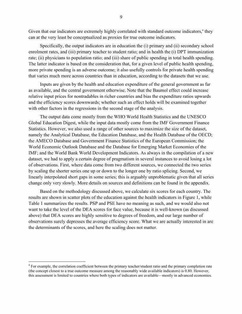
Given that our indicators are extremely highly correlated with standard outcome indicators,4 they can at the very least be conceptualized as proxies for true outcome indicators.

Specifically, the output indicators are in education the (i) primary and (ii) secondary school enrolment rates, and (iii) primary teacher to student ratio; and in health the (i) DPT immunization rate; (ii) physicians to population ratio; and (iii) share of public spending in total health spending. The latter indicator is based on the consideration that, for a given level of public health spending, more private spending is an adverse outcome; it also usefully controls for private health spending that varies much more across countries than in education, according to the datasets that we use.

Inputs are given by the health and education expenditure of the general government as far as available, and the central government otherwise. Note that the Baumol effect could increase relative input prices for nontradables in richer countries and bias the expenditure ratios upwards and the efficiency scores downwards; whether such an effect holds will be examined together with other factors in the regressions in the second stage of the analysis.

The output data come mostly from the WHO World Health Statistics and the UNESCO Global Education Digest, while the input data mostly come from the IMF Government Finance Statistics. However, we also used a range of other sources to maximize the size of the dataset, namely the Analytical Database, the Education Database, and the Health Database of the OECD; the AMECO Database and Government Finance Statistics of the European Commission; the World Economic Outlook Database and the Database for Emerging Market Economies of the IMF; and the World Bank World Development Indicators. As always in the compilation of a new dataset, we had to apply a certain degree of pragmatism in several instances to avoid losing a lot of observations. First, where data come from two different sources, we connected the two series by scaling the shorter series one up or down to the longer one by ratio splicing. Second, we linearly interpolated short gaps in some series; this is arguably unproblematic given that all series change only very slowly. More details on sources and definitions can be found in the appendix.

Based on the methodology discussed above, we calculate six scores for each country. The results are shown in scatter plots of the education against the health indicators in Figure 1, while Table 1 summarizes the results. PSP and PSE have no meaning as such, and we would also not want to take the level of the DEA scores for face value, because it is well-known (as discussed above) that DEA scores are highly sensitive to degrees of freedom, and our large number of observations surely depresses the average efficiency score. What we are actually interested in are the determinants of the scores, and here the scaling does not matter.

4 For example, the correlation coefficient between the primary teacher/student ratio and the primary completion rate (the concept closest to a true outcome measure among the reasonably wide available indicators) is 0.80. However, this assessment is limited to countries where both types of indicators are available—mostly in advanced economies.

10

Table 1. Summary of Scores

MeanCoefficient of

variation Minimum1st

quartile Median3rd

quartile Maximum

EducationPSPE 1.01 0.34 0.25 0.77 1.03 1.25 2.38PSEE 1.21 0.62 0.26 0.79 1.08 1.44 15.19DEAE 0.32 0.65 0.03 0.16 0.27 0.43 1.00HealthPSPH 1.15 0.28 0.23 0.93 1.23 1.41 1.81PSEH 1.38 0.64 0.53 0.89 1.10 1.54 8.04DEAH 0.34 0.63 0.08 0.18 0.25 0.45 1.00

Table 2. Spearman Rank Order Correlations

PSPE PSEE DEAE PSPH PSEH DEAH

Education PSPE 0.37 0.70 0.81 PSEE 0.37 0.83 0.37 -0.03 DEAE 0.70 0.83 0.10 -0.12Health PSPH 0.81 -0.20 -0.21 PSEH 0.37 -0.03 -0.20 0.63 DEAH 0.10 -0.12 -0.21 0.63

Education Health

Source: Authors’ calculations

Source: Authors’ calculations

11

Figure 1. Plots of PSP, PSE, and DEA Scores in Education and Health

0.5

11

.52

hea

lth

0 .5 1 1.5 2 2.5education

PSP

02

46

hea

lth

0 2 4 6 8education

PSE

0.2

.4.6

.81

hea

lth

0 .2 .4 .6 .8 1education

DEA

12

Figure 2. Evolution of Health and Education Spending, Performance, and Efficiency in Advanced and Developing Economies

Health Spending

0.0

1.0

2.0

3.0

4.0

5.0

6.0

7.0

1997 1998 1999 2000 2001 2002 2003

Advanced EconomiesDeveloping EconomiesAll

Education Spending

0.0

1.0

2.0

3.0

4.0

5.0

6.0

7.0

1980 1983 1986 1989 1992 1995 1998 2001

PSPH

0.7

0.8

0.9

1.0

1.1

1.2

1.3

1.4

1.5

1.6

1997 1998 1999 2000 2001 2002 2003

PSPE

0.7

0.8

0.9

1

1.1

1.2

1.3

1.4

1.5

1.6

1980 1983 1986 1989 1992 1995 1998 2001

PSEH

0.9

1

1.1

1.2

1.3

1.4

1.5

1.6

1.7

1.8

1.9

1997 1998 1999 2000 2001 2002 2003

PSEE

0.9

1

1.1

1.2

1.3

1.4

1980 1983 1986 1989 1992 1995 1998 2001

DEAH

0.1

0.2

0.3

0.4

0.5

1997 1998 1999 2000 2001 2002 2003

DEAE

0.1

0.2

0.3

0.4

0.5

1980 1983 1986 1989 1992 1995 1998 2001

Source: Authors’ calculations.

13

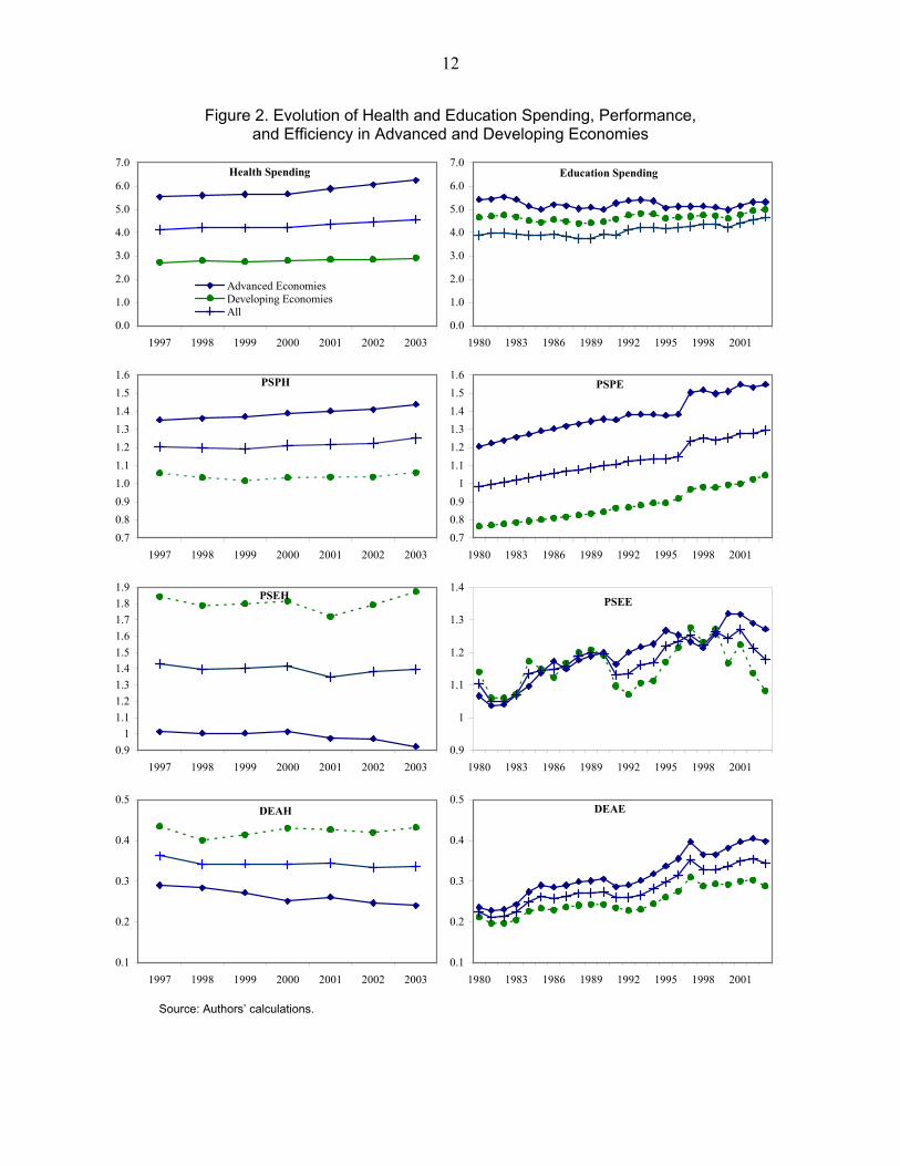
One interesting feature of the data is that education and health outputs are far more correlated than efficiency. In fact, as Table 2 shows, the correlation coefficient is 0.81 for PSP but only 0.37 for PSE, while it is even negative for DEA. Possibly related to this, the coefficient of variation for the two efficiency measures is about twice as large as for performance. And performance is positively correlated with efficiency for education, but negatively for health. It is possible that these features are explained by the greater relative cost-intensity of the provision of health care in richer countries. Indeed, as Figure 2 shows, while performance is highest in the advanced economies in both education and health, efficiency in these countries is also highest in education, but actually lowest in health.

It is also notable that not only performance, for which progress might have been expected, but also efficiency has trended upwards on average in each of three income groups. This is very clear in Figure 2, which is based on a stable set of countries. The figures for the education sector, which provide a longer horizon than those for the health sector, also reveal surprisingly large fluctuation of education spending relative to GDP, possibly reflecting cyclical factors. Volatility in spending spills over to the PSE/DEA scores, as outcomes are more stable.

We now proceed to the examination of the determinants of performance and efficiency.

IV. DETERMINANTS OF GOVERNMENT EFFICIENCY

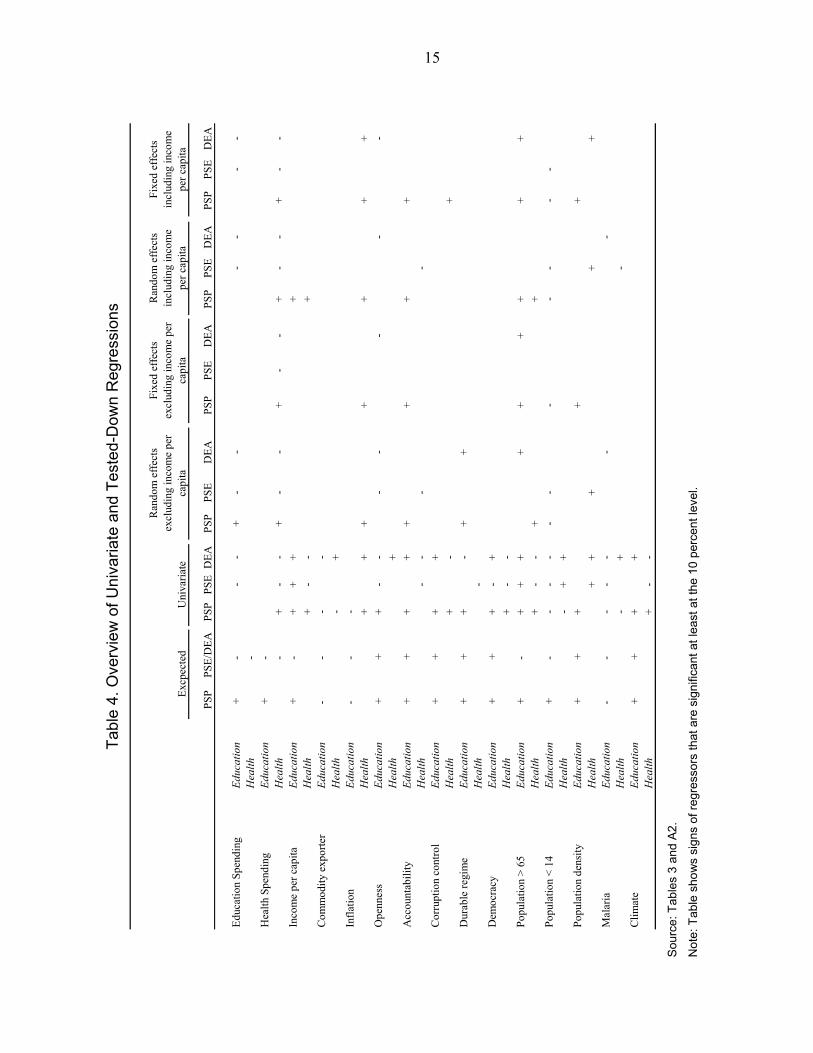
In this section, we relate the scores of public sector performance (PSP) and efficiency (PSE and DEA) to various potential correlates. Given the trade-off between the biases from omitted variables and high correlations between some of the regressors, we adopt a three-stage approach: we first run univariate regressions for all determinants, then combine those that are significant in multivariate regressions, and finally test these down by dropping all regressors that are not significant at least at the 10 percent level. For the sake of parsimony, we show in this section only the tested-down regressions (Table 3) and a table that summarizes from all regressions the signs of the regressors that are significant at least at the 10 percent level (Table 4). The other regressions, as well as definitions, sources, and descriptive statistics of the independent variables, most of which come from IMF and World Bank databases, can be found in the appendix. We group the discussion of the results by three categories of determinants: (i) economic; (ii) institutional; and (iii) demographic and geographic.

14

Table 3. Tested-Down Regressions

PSP PSE DEA PSP PSE DEA PSP PSE DEA PSP PSE DEAEducation spending Education 9.76E-03 -1.35E-01 -4.50E-02 -1.62E-01 -1.35E-01 -4.58E-02 -1.64E-01 -4.71E-02

(0.01) (0.00) (0.00) (0.00) (0.00) (0.00) (0.00) (0.00)Health

Health spending Education

Health 5.42E-02 -3.43E-01 -4.54E-02 4.49E-02 -3.57E-01 -5.57E-02 4.73E-02 -3.43E-01 -5.17E-02 4.53E-02 -3.58E-01 -4.85E-02(0.00) (0.00) (0.00) (0.00) (0.00) (0.00) (0.00) (0.00) (0.00) (0.00) (0.00) (0.00)

Income per capita Education 0.08 0.05 -0.59 0.10(0.00) (0.00) (0.11) (0.00)

Health 0.13 0.01(0.00) (0.59)

Commodity exporter Education

Health -8.02E-02 -7.17E-02(0.29) (0.29)

Inflation Education 5.79E-04(0.00)

Health 2.50E-04 4.16E-04 3.30E-04 4.76E-04 1.13E-04 3.55E-04 4.16E-04 2.14E-04 5.17E-04 1.37E-04(0.00) (0.00) (0.00) (0.00) (0.00) (0.00) (0.00) (0.00) (0.00) (0.00)

Openness Education -3.78E-05 -1.24E-05 -2.68E-05 -3.78E-05 -1.79E-05 -2.21E-05(0.03) (0.02) (0.00) (0.03) (0.00) (0.00)

Health -9.67E-06 -1.31E-05(0.32) (0.09)

Accountability Education 4.57E-02 -1.84E-01 3.28E-02 3.20E-01 2.40E-02 -1.84E-01 4.98E-02 1.04E-01(0.02) (0.09) (0.02) (0.04) (0.09) (0.09) (0.00) (0.26)

Health -1.29E-01 -7.15E-02 -1.29E-01(0.01) (0.25) (0.01)

Corruption control Education -9.62E-02 -8.03E-02 -9.62E-02(0.02) (0.25) (0.02)

Health 9.60E-03 4.25E-02 3.03E-02 9.76E-02 5.01E-02(0.38) (0.08) (0.02) (0.05) (0.04)

Durable regime Education 1.00E-03 8.04E-04 -1.81E-02 9.03E-04 5.20E-04 1.05E-04(0.03) (0.00) (0.04) (0.09) (0.23) (0.74)

Health

Democracy Education -2.42E-03 -4.37E-02 -2.08E-03 -1.70E-03 -2.12E-03(0.05) (0.18) (0.11) (0.09) (0.04)

Health -5.13E-03 -1.30E-03 -2.82E-03 -9.41E-04(0.04) (0.00) (0.00) (0.69)

Population > 65 Education 9.75E-03 1.74E-02 2.28E-02 2.61E-02 1.24E-02 1.84E-02 2.06E-02 1.27E-02(0.11) (0.00) (0.00) (0.00) 0.044 (0.00) (0.06) (0.00)

Health 3.36E-02 6.43E-02 -1.20E-02 2.45E-02 2.27E-02 6.43E-02 -2.35E-02(0.00) (0.00) (0.78) (0.32) (0.00) (0.00) (0.58)

Population < 14 Education -2.09E-02 -5.04E-02 -1.56E-02 -7.84E-02 6.06E-03 -1.48E-02 -5.04E-02 4.60E-02 -1.01E-01 5.78E-03(0.00) (0.00) (0.00) (0.00) (0.02) (0.00) (0.00) (0.00) (0.00) (0.02)

Health -1.06E-03 -3.66E-03 2.08E-02 -2.15E-02(0.62) (0.05) (0.00) (0.05)

Population density Education 1.35E-03 -5.45E-05 -3.83E-05 1.72E-03 -1.49E-04

(0.00) (0.03) (0.00) (0.00) (0.00)

Health 1.34E-04 2.71E-05 1.21E-04 1.34E-04 -1.21E-04

(0.05) (0.85) (0.32) (0.05) (0.03)Malaria Education -6.84E-03 -6.37E-03

(0.00) (0.01)Health -1.44E-02 -3.42E-02 -3.42E-02

(0.00) (0.00) (0.00)Climate Education -1.01E+00 -1.01E+00 -1.83E-01

(0.02) (0.02) (0.14)Health

Adjusted R2 Education 0.78 0.20 0.45 0.15 0.06 0.22 0.78 0.20 0.49 0.41 0.09 0.23Health 0.78 0.52 0.17 0.48 0.32 0.02 0.65 0.52 0.15 0.28 0.30 0.00

Endogneity test p a

Education 0.01 0.11 0.21 n.a. 0.91 n.a. 0.18 0.11 0.28 n.a. 0.72 0.26Health 0.05 0.33 0.04 0.04 0.02 0.01 0.44 0.33 0.63 0.08 0.01 0.21

Random effects including income per capita

Fixed effects including income per capita

Random effects excluding income per capita

Fixed effects excluding income per capita

Source: Authors’ calculations.

Notes: All regressions include a constant that is not reported. Heteroskedasticity-robust p-values in parentheses. a p-values(s) of coefficients on residuals from auxiliary regressions added to regressors (see text for test procedure)

15

Tab

le 4

. O

verv

iew

of U

niva

riate

and

Tes

ted-

Dow

n R

egre

ssio

ns

PS

PP

SE/D

EA

PSP

PSE

DE

AP

SPP

SED

EA

PSP

PSE

DE

AP

SP

PS

ED

EA

PS

PP

SE

DE

A

Edu

catio

n Sp

endi

ngE

duca

tion

+

-

--

+-

--

--

-H

ealth

-

Hea

lth

Spen

ding

Edu

cati

on+

-

H

ealth

-

+-

-+

--

+-

-+

--

+-

-In

com

e pe

r ca

pita

Edu

cati

on+

-

+

++

+H

ealth

+-

-+

Com

mod

ity

expo

rter

Edu

cati

on-

-

-

-H

ealth

-+

Infl

atio

nE

duca

tion

-

-

-H

ealth

++

++

++

+O

penn

ess

Edu

cati

on+

+

+

--

--

--

-H

ealth

+A

ccou

ntab

ility

Edu

cati

on+

+

+

++

++

+H

ealth

--

--

Cor

rupt

ion

cont

rol

Edu

cati

on+

+

+

+H

ealth

+-

+D

urab

le r

egim

eE

duca

tion

+

+

+-

++

Hea

lth-

Dem

ocra

cyE

duca

tion

+

+

+-

+H

ealth

+-

-P

opul

atio

n >

65

Edu

cati

on+

-

+

++

++

++

++

Hea

lth+

--

++

Pop

ulat

ion

< 1

4E

duca

tion

+

-

--

--

--

--

--

Hea

lth-

++

Pop

ulat

ion

dens

ityE

duca

tion

+

+

++

+H

ealth

++

++

+M

alar

iaE

duca

tion

-

-

--

--

-H

ealth

-+

-C

lim

ate

Edu

cati

on+

+

+

+H

ealth

+-

-

Fix

ed e

ffec

ts

incl

udin

g in

com

e pe

r ca

pita

Uni

vari

ate

Ran

dom

eff

ects

ex

clud

ing

inco

me

per

capi

ta

Fix

ed e

ffec

ts

excl

udin

g in

com

e pe

r ca

pita

Ran

dom

eff

ects

in

clud

ing

inco

me

per

capi

taE

xcpe

cted

S

ourc

e: T

able

s 3

and

A2.

Not

e: T

able

sho

ws

sig

ns o

f reg

ress

ors

that

are

sig

nifi

cant

at

leas

t at t

he 1

0 p

erce

nt le

vel.

16

A. Economic Determinants

Our most resounding result is that larger education and health spending reduces public sector efficiency in each of the sectors, and in education does not even bear a significant relationship with public sector performance. In other words, citizens on average get declining marginal improvements in performance for increasing public funding of education and health and no improvement at all in education. The result that higher spending leads to lower efficiency is in line with other studies: for example, Hauner (2008) found the same for Russia’s regions. This contrasts with the finding in La Porta et al. (1999) that larger governments perform better, but they focus on performance in absolute terms (similar to our public sector performance measure) and do not take the cost to the public purse into account.

There could be endogeneity, however, if lower efficiency leads to higher spending relative to GDP. Augmented regression tests,5 whose p-values are shown below the coefficients in Table 3, do not suggest such endogeneity in the education efficiency regressions, but they do for health efficiency (whether measured by PSE or DEA), implying evidence that lower efficiency leads to higher spending. To further investigate the direction of causality, we run the same specification with the two-step system GMM estimator of Arellano and Bover (1995) and Blundell and Bond (1998).6 The results, which are available on request, are not clear: for PSE, we find a significant negative effect confirming the OLS result; for DEA, the coefficient on health expenditure becomes insignificant. We conclude, however, that while the direction of causality in the relationship between health expenditure and health efficiency remains somewhat unclear, this does not change the more general finding that there is a nexus between higher expenditure and lower efficiency. This observation has important policy implications as we will discuss in the concluding section.

The effect of income per capita could go both ways. It could, on the one hand, reduce efficiency by raising the relative cost of public services (Baumol, 1967). On the other hand, higher income has often been found to be associated with better health and education outcomes (Afonso and Aubyn, 2006; Afonso et al., 2006; Herrera and Pang, 2005), while, on the other hand, poorer countries have been found to exhibit inferior government performance (La Porta et al., 1999). Our results, while not entirely conclusive, provide more support for

5 The potentially endogenous variables are regressed on a constant and all other variables. The residuals from these regressions are included as additional regressors in the tested-down specification. If the coefficient on a residual is significantly different from zero, the null hypothesis that the variable is exogenous is rejected. 6 System GMM estimates in a system the equations in differences and levels, each with its specific set of instruments. Relative to conventional instrumental variable methods, it improves substantially on the weak instruments problem through more formal checks of the validity of the instruments and provides for potentially improved efficiency. We apply the Windmeijer (2005) correction to the reported standard errors. Lag length selection is guided by the Arellano-Bond and Hansen tests. We use the maximum possible number of up to six lags in almost all cases. We collapse the instruments to limit their number. As the Hansen test becomes weak when instruments are many, we limit the number of instruments to the number of groups. We include time dummies as they make the required assumption of no correlation across groups in the idiosyncratic disturbances more likely to hold, and use orthogonal deviations to maximize sample size in our panel with many gaps.

17

the second hypothesis, as the signs of several of the significant coefficients in the tested-down regressions are positive, while the negative signs that appear in several of the univariate and multivariate specifications disappear when the specification is tested down. While income per capita could be endogenous if public sector performance and efficiency affects growth, augmented regression tests, whose p-values again appear below the coefficients in Table 3, suggest that the effect of income level is in fact exogenous.

To allow for non-linear effects related to income level we try also a dummy for developing countries, but it is never significant. Another dummy marks commodity exporters that could be expected to have lower public sector performance and efficiency, as the income level in these cases tends to overstate the overall level of economic and institutional development, and as commodity windfalls may negatively affect incentives in the public sector (Desai et al., 2005). The results in the univariate regressions are overall in line with this presumption, but the dummy becomes insignificant in the multivariate regressions.

We would have expected higher inflation to negatively affect efficiency as it complicates economic planning, but surprisingly the effect is in most cases positive in the health sector, although it is insignificant in education. However, the explanation may lie in a mundane detail of the budget process in many countries: if inflation is higher than expected in the budget, and there is no supplementary budget to raise spending limits, the expenditure/GDP ratio—the denominator of the efficiency scores—will be lower than intended by policy. This would tend to lead to a scramble for resources as the public sector is squeezed in real terms. This could—as long as inflation is a surprise—improve efficiency.

Openness could be expected to increase performance and efficiency by increasing competitive pressure on the domestic economy, including the government, as well as raising more generally exposure to the outside world, including through skills and technology transfer. We look both at de jure trade liberalization and de facto openness, but none of them turn out significant in the final tested-down specification.

B. Institutional Determinants

Institutions have become well-established as determinants of economic growth and financial development. It is quite likely that they also determine the efficiency of government. For example, Putnam (1993) and Gellner (1994) have argued that the degree of development of civil society influences the effectiveness of the public sector: cooperation between citizens and their formation of non-state institutions enables them to exert more effective control over politicians and bureaucrats. Indeed, we find that higher accountability of the government highly consistently increases education performance. A less intuitive—albeit not very robust—result is that higher accountability reduces health sector efficiency.

Control of corruption is a very intuitive determinant of efficiency, given that corruption breeds waste. Moreover, it is well-established that corruption is bad for growth (Mauro, 1995). And indeed, there is very robust evidence that controlling corruption

18

increases efficiency, but also performance, in both the education and health sectors. The fact that these results appear in the tested-down regressions only when we control for country effects and per capita income makes actually makes the conclusion more credible.

Several other institutional variables that we examine are not significant. This includes first the degree of democracy where higher scores could have been expected to increase government accountability. Moreover, we try the durability of governments as higher volatility would be expected to complicate consistent budgetary planning and undermine efficiency. Finally, we examine the effects of social infrastructure and years of schooling that have been used by Hall and Jones (1999) as determinants of economic growth, under the presumption that a tighter social fabric and a more educated population contribute to greater performance and efficiency through more successful monitoring of the government. Moreover, education levels have been shown by Afonso et al. (2006) to increase health sector efficiency; note that we do not include this variable in the regressions for the education sector because of the obvious endogeneity with respect to education performance and efficiency.

C. Demographic and Geographic Determinants

Establishing robust results on economic and institutional determinants requires controlling for a number of “environmental” factors that can be expected to affect the performance and efficiency of government.

Given that we are specifically looking at education and health, one obvious candidate is the age distribution of the population: a younger population could be expected to increase the cost of the education system relative to outcome indicators that do not take the size of the current student population into account; in contrast, an older population could be expected to have the same effect in the health sector. In the education sector, there is indeed robust evidence that a younger population reduces, while an older population increases efficiency. Less intuitive is that also performance seems to suffer in this case; this could possibly due to negative implications of a more crowded school system. In the health sector, the share of the younger population does not seem to matter much. In contrast, there is some evidence of a positive effect of the elderly population on both health performance and efficiency. Note that our health outcomes do not include measures of life expectancy, whose influence could have been the most straightforward explanation for this unexpected result, given that an older population obviously correlates with higher life expectancy.

Higher population density can be expected to improve public sector performance and efficiency by reducing the cost of service provision through economies of scale and lower transportation and heating costs. Indeed, we find some evidence of such a positive effect. However, linguistic fractionalization, which could make it more expensive and difficult to deliver public services due to communication problems and may increase the need for potentially efficiency-reducing redistributive policies (Alesina et al., 1999; Easterly and

19

Levine, 1997), does not yield any significant results.7 This stands in contrast to the finding in La Porta et al. (1999) that higher linguistic fractionalization reduces quality of government.

Finally, climate could be expected to affect public sector performance and efficiency in education and health through various channels: for example, some areas are more prone to malaria, irrespective of the level of health services, while schools and hospitals have high heating costs (which show up in education and health spending) in other areas of the world. We capture these factors through an ecologically-based spatial index of malaria stability and the distance from the equator as a proxy for climate. However, none of these factors shows significant effects in the final tested-down regression specifications. This contrasts with the finding of La Porta et al. (1999) that countries close to the equator exhibit inferior government performance; however, their regression specifications are not comparable with ours as they control for per capita income, while we estimate a larger multivariate regression.

V. CONCLUSIONS

We have undertaken the first examination of the determinants of government efficiency with a large country panel, building on a newly compiled dataset of scores of public sector performance and efficiency in education and health around the world. Our results have two key policy implications. First, the strong evidence that efficiency declines with the level of spending, and that, at least in education, there is not even a significant relationship between performance and spending, highlight what should be commonly accepted wisdom but is often ignored in policymaking: throwing money at problems, particularly in the education and health sectors that we studied here, often fails to yield the expected improvement in public services if not bolstered by efficiency-increasing policies. Second, the benefits of improving institutions extend from economic growth and financial development, to government efficiency. We find that particularly government accountability and controlling corruption can play a positive role. We also find that demographic and geographic factors matter, but these governments will have to take as a given—for better or for worse.

7 Language fractionalization has often been used as an instrument. Here, we use it simply as a regressor.

20

VI. APPENDIX

A. Data Sources

We use the following acronyms: ADB…OECD Analytical Database; AMECO…European Commission Ameco Database; EDUDB…OECD Education Database; EUGFS…European Commission Government Finance Statistics; DEME…IMF Database for Emerging Market Economies; HELDB…OECD Health Database; WDI… World Bank World Development Indicators; WEO…IMF World Economic Outlook Database; WHO…World Health Statistics. Identifiers of the series in the respective database, if available, are in parentheses. Where several sources were used, they are mentioned in the order of their share in the data.

Outputs: primary school enrolment: WDI (SEPRMENRR); secondary school enrolment: WDI (SESECENRR); primary teacher/student ratio: WDI (SEPRMENRLTCZS); share of public health spending: WDI (SHXPDPRIVZS) and HELDB; immunization rate DPT: WDI (SHIMMIDPT); physicians per 1,000 people: WDI (SHMEDPHYSZS) and HELDB.

Inputs: education spending: WDI (SEXPDTOTLGDZS), Eurostat, and EDUDB; health spending: WDI (SHXPDPUBLZS), HELDB, WHO, AMECO, and GFS (aB_GG_707); nominal GDP: WEO (NGDP).

Economic determinants: Education spending and health spending are the respective spending in percent of GDP; see description of inputs above. Income per capita is measured in logs and PPP and comes from the WEO. Commodity exporter and developing country are dummies using the IMF World Economic Outlook classification. Inflation is the CPI inflation rate from the same source. Trade liberalization is measured by average tariff rates, coming from Hauner and Prati (2008). Openness is defined as the sum of imports and exports over GDP and comes from the WEO.

Institutional determinants: Accountability and corruption control range from 0 to 100, where higher values are better, and come from the World Bank’s “Governance Matters” dataset available at info.worldbank.org/governance/wgi2007. Democracy ranges from -10 (high autocracy) to +10 (high democracy) and comes from the Polity IV dataset available at www.cidcm.umd.edu/polity/. Durable regime measures the number of years since the last change in the political regime and comes from the same dataset. Social infrastructure is the average of an index of government anti-diversion policies and an index of trade openness, as defined by Hall and Jones (1999). Schooling (which is only a regressor in the health regressions) also comes from the Hall and Jones (1999) dataset.

Demographic and geographic determinants: Population >65 and Population <14 are the share of the population above and below that age, respectively, and come from the WDI. Population density also comes from the WDI. Fractionalization assumes higher values if more languages are present in a given country, ranging from 0 to 1, and coming from the Encyclopedia Britannica. Malaria is an ecologically-based spatial index of stability of malaria transmission, ranging from 0 to 31.5, from the Gordon McCord Malaria Dataset, Earth Institute at Columbia University. Climate is proxied by distance from the equator,

21

measures by the absolute value of latitude in degrees divided by 90 to place it on a 0 to 1 scale from the Hall and Jones (1999) dataset.

B. Countries Included

Advanced economies: Australia, Austria, Belgium, Canada, Denmark, Finland, France, Germany, Greece, Hong Kong, Ireland, Italy, Japan, Korea Rep., Luxemburg, Netherlands, New Zealand, Norway, Portugal, Singapore, Spain, Sweden, Switzerland, Taiwan, United Kingdom, United States.

Developing economies: Albania, Algeria, Antigua & Barbuda, Argentina, Armenia, Azerbaijan, Bangladesh, Belarus, Benin, Bolivia, Botswana, Brazil, Bulgaria, Burkina Faso, Cambodia, Cameroon, Central African Republic, Chad, Chile, China, Colombia, Costa Rica, DR Congo, Cote d'Ivoire, Croatia, Cyprus, Czech Rep., Dominican Rep., Ecuador, Egypt, El Salvador, Estonia, Ethiopia, Georgia, Ghana, Guatemala, Honduras, Hungary, India, Israel, Indonesia, Jamaica, Jordan, Kazakhstan, Kenya, Kyrgyz Rep., Latvia, Lebanon, Lithuania,

Madagascar, Malaysia, Malawi, Mali, Mexico, Moldova, Morocco, Mozambique, Myanmar, Namibia, Nepal, Nicaragua, Niger, Nigeria, Pakistan, Paraguay, Peru, Philippines, Poland,

Romania, Russia, Saudi Arabia, Senegal, South Africa, Sri Lanka, Tajikistan, Tanzania, Thailand, Togo, Tunisia, Turkey, Uganda, Ukraine, Uruguay, Uzbekistan, Venezuela, Vietnam, Zambia, Zimbabwe.

C. Background Tables

Table A1. Summary of Determinants

MeanCoefficient of variation Minimum

1st quartile Median

3rd quartile Maximum

Education spending 4.3 0.4 0.1 2.8 4.3 5.5 11.0Health spending 4.1 0.5 0.3 2.3 4.1 5.6 9.6Income per capita 8.4 0.1 5.7 7.4 8.4 9.3 11.3Inflation 62.1 8.7 -77.2 2.7 6.9 15.9 15606.5Trade Liberalization 0.8 0.1 0.0 0.8 0.9 0.9 1.0Openess 60.4 0.6 0.0 36.2 53.8 74.5 297.3Accountability 0.1 14.5 -2.2 -0.6 0.0 0.9 1.7Corruption control 0.1 12.2 -1.8 -0.8 -0.3 0.8 2.5Durable regime 25.1 1.3 0.0 4.0 13.0 35.0 195.0Democracy 2.8 2.5 -10.0 -5.0 6.0 9.0 10.0Social infrastructure 0.5 0.5 0.2 0.3 0.4 0.8 1.0Schooling 5.2 0.5 0.5 3.1 4.8 7.0 12.0Population > 65 7.4 0.6 2.0 3.4 5.0 11.7 20.2Population < 14 32.5 0.3 13.5 21.7 33.6 42.6 50.5Population density 191.0 3.8 1.2 23.9 60.8 123.1 6728.4Fractionalization 0.4 0.8 0.0 0.1 0.4 0.6 0.9Malaria 3.6 1.9 0.0 0.0 0.1 4.1 31.5Climate 0.3 0.6 0.0 0.1 0.3 0.4 0.7

22

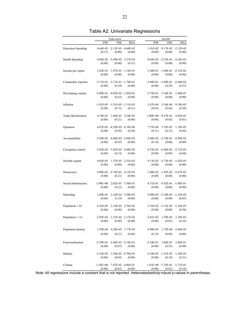
Table A2. Univariate Regressions

PSP PSE DEA PSP PSE DEA

Education Spending 4.64E-03 -2.13E-01 -4.68E-02 1.91E-02 -9.17E-02 -2.12E-02(0.17) (0.00) (0.00) (0.00) (0.00) (0.00)

Health Spending 4.04E-02 -5.49E-02 3.27E-03 8.64E-02 -2.25E-01 -4.16E-02(0.00) (0.00) (0.51) (0.00) (0.00) (0.00)

Income per capita 2.42E-01 1.07E-01 1.14E-01 2.30E-01 -1.04E-01 -2.31E-02(0.00) (0.00) (0.00) (0.00) (0.00) (0.06)

Commodity exporter -3.71E-01 -3.71E-01 -1.74E-01 -3.88E-01 -1.89E-01 -2.66E-02(0.00) (0.18) (0.00) (0.00) (0.28) (0.53)

Developing country -5.00E-01 -4.02E-02 -1.82E-01 -3.75E-01 5.16E-01 1.48E-01(0.00) (0.62) (0.00) (0.00) (0.00) (0.00)

Inflation -1.01E-05 -1.51E-05 -1.11E-05 1.67E-04 3.16E-04 9.19E-05(0.00) (0.71) (0.31) (0.03) (0.44) (0.30)

Trade liberalization 4.19E-01 1.66E-01 2.24E-01 1.00E+00 -9.57E-01 -3.03E-01(0.00) (0.21) (0.00) (0.00) (0.02) (0.01)

Openness 4.67E-05 -6.29E-05 6.10E-06 7.75E-06 3.35E-05 1.19E-05(0.00) (0.02) (0.38) (0.51) (0.15) (0.04)

Accountability 9.30E-02 -6.60E-02 6.88E-02 2.60E-02 -2.74E-01 -5.99E-02(0.00) (0.43) (0.00) (0.14) (0.00) (0.00)

Corruption control 5.65E-02 -7.83E-02 4.84E-02 4.72E-02 -6.48E-02 -2.71E-02(0.00) (0.13) (0.00) (0.00) (0.09) (0.04)

Durable regime 4.02E-03 1.57E-03 2.21E-03 9.13E-03 -5.73E-03 -1.62E-03(0.00) (0.08) (0.00) (0.00) (0.00) (0.00)

Democracy 9.08E-03 -5.76E-03 4.13E-03 1.00E-02 -1.93E-02 -5.67E-03(0.00) (0.21) (0.00) (0.00) (0.00) (0.00)

Social infrastructure 1.04E+00 2.02E-01 3.58E-01 8.71E-01 -5.42E-01 -1.96E-01(0.00) (0.22) (0.00) (0.00) (0.00) (0.00)

Schooling 1.09E-01 2.16E-02 3.58E-02 9.08E-02 -5.10E-02 -1.32E-02(0.00) 0.134 (0.00) (0.00) (0.00) (0.03)

Population > 65 6.36E-02 2.14E-02 2.76E-02 5.55E-02 -3.13E-02 -1.54E-03(0.00) (0.00) (0.00) (0.00) (0.00) (0.58)

Population < 14 -2.95E-02 -1.31E-02 -1.17E-02 -2.81E-02 1.59E-02 2.10E-03(0.00) (0.00) (0.00) (0.00) (0.01) (0.16)

Population density 1.59E-04 4.28E-05 1.77E-05 8.90E-05 1.75E-04 3.48E-05

(0.00) (0.21) (0.04) (0.19) (0.09) (0.00)

Fractionalization -5.59E-01 -3.46E-01 -2.14E-01 -5.24E-01 1.86E-01 1.06E-01(0.00) (0.07) (0.00) (0.00) (0.55) (0.09)

Malaria -3.16E-02 -1.54E-02 -9.79E-03 -3.24E-02 -1.51E-02 1.54E-03(0.00) (0.03) (0.00) (0.00) (0.19) (0.51)

Climate 1.54E+00 7.47E-02 4.86E-01 1.41E+00 -7.35E-01 -1.71E-01(0.00) (0.83) (0.00) (0.00) (0.01) (0.10)

Education Health

Note: All regressions include a constant that is not reported. Heteroskedasticity-robust p-values in parentheses.

23

Table A3. Multivariate Regressions

PSP PSE DEA PSP PSE DEA PSP PSE DEA PSP PSE DEA

Education Spending Education 9.34E-03 -1.35E-01 -4.46E-02 1.88E-03 -1.64E-01 -0.04458 6.03E-03 -1.35E-01 -4.55E-02 2.75E-03 -1.47E-01 -4.55E-02(0.02) (0.00) (0.00) (0.67) (0.00) (0.00) (0.13) (0.00) (0.00) (0.53) (0.00) (0.00)

Health

Health Spending Education -3.76E-01 -3.74E-01(0.00) (0.00)

Health 4.44E-02 -3.76E-01 -5.96E-02 4.56E-02 -0.38418 -5.45E-02 4.17E-02 -5.42E-02 4.64E-02 -4.22E-02(0.00) (0.00) (0.00) (0.00) (0.00) (0.00) (0.00) (0.00) (0.00) (0.00)

Income per capita Education 8.97E-02 1.06E-02 5.59E-02 -5.74E-02 -1.23E+00 8.14E-02(0.00) (0.87) (0.00) (0.29) (0.08) (0.00)

Health 1.04E-01 -3.48E-02 -7.74E-02 6.34E-02 4.24E-01 -1.55E-02(0.00) (0.75) (0.00) (0.31) (0.26) (0.86)

Commodity exporter Education

Health -1.47E-01 -1.63E-01(0.02) (0.00)

Inflation Education -1.74E-06 5.64E-04 -1.21E-05(0.94) (0.00) (0.23)

Health 2.24E-04 4.70E-04 2.12E-04 4.81E-04 1.33E-04 2.24E-04 4.69E-04 2.14E-04 5.02E-04 1.33E-04(0.00) (0.00) (0.00) (0.00) (0.00) (0.00) (0.00) (0.00) (0.00) (0.00)

Openness Education 7.09E-07 -6.93E-05 -1.39E-05 -7.27E-06 -2.25E-04 -2.64E-05 -6.37E-06 -6.93E-05 -1.88E-05 -5.45E-06 -6.61E-05 -2.26E-05(0.91) (0.13) (0.00) (0.36) (0.14) (0.00) (0.38) (0.13) (0.00) (0.52) (0.43) (0.00)

Health -1.64E-05 -2.32E-05 -7.23E-06 -7.07E-07 3.26E-06 -1.91E-05 -2.10E-05 -8.80E-06 -8.12E-06(0.09) (0.35) (0.54) (0.98) (0.76) (0.04) (0.44) (0.47) (0.79)

Accountability Education 5.09E-02 -4.55E-02 4.69E-02 3.77E-01 3.98E-02 -4.55E-02 4.44E-02 2.55E-01(0.00) (0.69) (0.01) (0.02) (0.01) (0.69) (0.07) (0.07)

Health -1.12E-01 2.71E-03 -1.09E-01 -2.10E-02 -1.07E-01 1.59E-02 -1.09E-01 3.32E-03(0.03) (0.89) (0.01) (0.57) (0.05) (0.43) (0.11) (0.91)

Corruption control Education -1.46E-01 -2.98E-02 -1.46E-01 -5.95E-02(0.00) (0.59) (0.00) (0.39)

Health 1.52E-02 8.61E-04 2.02E-02 3.45E-02 3.45E-03 2.16E-02 2.19E-02 3.32E-02(0.13) (0.96) (0.11) (0.17) (0.70) (0.22) (0.09) (0.11)

Durable regime Education 1.03E-03 5.68E-04 1.11E-04 -2.67E-02 9.09E-04 2.39E-04 9.60E-05 3.44E-04 2.68E-04(0.02) (0.05) (0.85) (0.04) (0.09) (0.59) (0.75) (0.57) (0.58)

Health 1.64E-03 8.56E-03 1.93E-03 8.32E-03(0.44) (0.13) (0.41) (0.15)

Democracy Education -2.28E-03 -2.15E-02 -1.25E-03 -1.95E-03 -5.98E-02 -2.03E-03 -2.94E-03 -2.15E-02 -1.68E-03 -1.90E-03 -3.51E-02 -1.26E-03(0.08) (0.32) (0.22) (0.15) (0.15) (0.20) (0.03) (0.30) (0.01) (0.17) (0.30) (0.30)

Health -5.29E-03 -1.75E-03 -3.24E-03 -6.26E-04 -5.81E-03 -2.44E-03 -3.37E-03 -3.12E-03(0.08) (0.39) (0.33) (0.83) (0.04) (0.24) (0.32) (0.19)

Population > 65 Education 1.43E-02 2.22E-02 2.61E-02 2.61E-02 1.37E-02 2.08E-02 2.80E-02 1.76E-02(0.04) (0.00) (0.06) (0.00) (0.04) (0.00) (0.06) (0.00)

Health 2.76E-02 -2.32E-05 3.91E-03 2.77E-03 -4.87E-03 3.56E-02 2.99E-02 6.36E-02 -1.17E-03 4.06E-04 -2.83E-02 2.43E-02(0.00) (0.35) (0.61) (0.81) (0.93) (0.07) (0.00) (0.00) (0.88) (0.97) (0.46) (0.43)

Population < 14 Education -1.87E-02 -5.30E-02 2.79E-04 -1.08E-02 -3.88E-02 6.10E-03 -1.34E-02 -5.30E-02 1.93E-03 -1.32E-02 -9.93E-02 6.04E-03(0.00) (0.00) (0.89) (0.05) (0.14) (0.02) (0.00) (0.00) (0.36) (0.05) (0.02) (0.02)

Health -2.41E-03 -3.83E-03 2.27E-02 -1.32E-02 3.36E-03 -9.16E-03 2.47E-02 -3.87E-02(0.48) (0.39) (0.00) (0.19) (0.30) (0.06) (0.00) (0.00)

Population density Education 9.85E-05 -1.64E-05 1.77E-03 -5.40E-05 9.91E-05 -3.21E-05 1.75E-03 -9.91E-05

(0.53) (0.29) (0.00) (0.03) (0.49) (0.05) (0.00) (0.00)

Health -2.22E-06 1.23E-04 8.95E-06 -1.36E-04 -9.46E-05 1.19E-04 -1.82E-05 1.33E-04 1.29E-05 -1.28E-04 -2.78E-05 7.53E-05

(0.92) (0.08) (0.59) (0.01) (0.82) (0.34) (0.44) (0.08) (0.43) (0.01) (0.95) (0.44)Fractionalization Education -3.81E-02 -7.93E-03

(0.49) (0.89)Health -2.12E-01 -1.79E-01

(0.00) (0.00)Malaria Education -7.46E-03 -1.82E-05 -6.48E-03

(0.00) (0.44) (0.00)Health -5.66E-03 -4.08E-02 1.84E-03 -3.50E-03 -4.22E-02 1.29E-03

(0.13) (0.00) (0.43) (0.28) (0.00) (0.55)Climate Education -1.02E-01 -1.15E+00 -1.71E-01

(0.45) (0.00) (0.20)Health 1.36E-01 4.75E-02 -7.03E-03 9.89E-02

(0.40) (0.77) (0.96) (0.52)

Adjusted R2 Education 0.79 0.20 0.47 0.46 0.03 0.21 0.81 0.20 0.49 0.41 0.05 0.36

Health 0.88 0.50 0.31 0.27 0.28 0.00 0.89 0.51 0.34 0.17 0.14 0.02

Random effects including income per capita

Fixed effects including income per capita

Random effects excluding income per capita

Fixed effects excluding income per capita

Note: All regressions include a constant that is not reported. Heteroskedasticity-robust p-values in parentheses.

24

REFERENCES

Afonso, A., Aubyn, St., 2006. Cross-country efficiency of secondary education provision: a semi-parametric analysis with non-discretionary inputs. Economic Modelling 23, 476–491.

Afonso, A., Schuknecht, L., Tanzi, V., 2005. Public sector efficiency: an international comparison. Public Choice 123, 312–347.

Afonso, A., Schuknecht, L., Tanzi, V., 2006. Public sector efficiency: evidence for the new EU member states and emerging markets. Working paper no. 581, European Central Bank, Frankfurt, Germany.

Alesina, A., Baqir, R., Easterly, W., 1999. Public goods and ethnic divisions. Quarterly Journal of Economics 114, 1243–1284.

Arellano, M., Bover, O., 1995. Another look at the instrumental variables estimation of error-component models. Journal of Econometrics 68, 29–51.

Baumol, W.J., 1967. Macroeconomics of unbalanced growth: the anatomy of the urban crisis. American Economic Review 57, 415–426.

Blundell, R., Bond, S., 1998. Initial conditions and moment restrictions in dynamic panel data models. Journal of Econometrics 87, 115–143.

Debreu, G., 1951. The coefficient of resource utilization. Econometrica 19, 273–292.

Desai, R.M., Freinkman, L., Goldberg, I., 2005. Fiscal federalism in rentier regions: evidence from Russia. Journal of Comparative Economics 33, 641–654.

Easterly, W., Levine, R., 1997. Africa’s growth tragedy: policies and ethnic divisions. Quarterly Journal of Economics 112, 1203–1250.

Färe, R., Grosskopf, S., Lovell, C.A.K., 1994. Production frontiers. Cambridge: Cambridge University Press.

Farrell, M. J., 1957. The Measurement of productive efficiency. Journal of the Royal Statistical Society 20 (Series A), 253–281.

Friedman, E., Johnson, S., Kaufmann, D., Zoido-Lobaton, P., 2000. Dodging the grabbing hand: the determinants of unofficial activity in 69 countries. Journal of Public Economics 76, 459–493.

Gellner, E., 1994. Conditions of liberty: civil society and its rivals. Harmondsworth: Allen Lane/Penguin Press.

Gupta, S., Verhoeven, M., 2001. The efficiency of government expenditure: experiences from Africa. Journal of Policy Modeling 23, 433–467.

25

Hall, R.E., Jones, Ch.I., 1999. Why do some countries produce so much more output per worker than others? Quarterly Journal of Economics 114, 83–116.

Hauner, D., 2008. Explaining differences in public sector efficiency: evidence from Russia’s regions. World Development, forthcoming.

Hauner, D., Prati, A., 2008. The interest rate theory of financial development: evidence from regulation. IMF Working Paper, forthcoming.

Heller, P., Hauner, D., 2006. Fiscal policy in the face of long-term expenditure uncertainties. International Tax and Public Finance 13, 325–350.

Herrera, S., Pang, G., 2005. Efficiency of public spending in developing countries: an efficiency frontier approach. Policy research working paper no. 3645, World Bank, Washington, DC.

La Porta, R., Lopez-de-Silanes, F., Shleifer, A., and Vishny R.W., 1999. The quality of government. Journal of Law, Economics, and Organization 15, 222–279.

Mauro, P., 1995. Corruption and growth. Quarterly Journal of Economics 110, 681–712.

Putnam, R.D., 1993. Making democracy work: Civic traditions in modern Italy. Princeton: Princeton University Press.

Seiford, L. M., Thrall, R. M., 1990. Recent developments in DEA: the mathematical programming approach to frontier analysis. Journal of econometrics 46, 7–38.

Simar, L., Wilson, P.W., 2007. Estimation and inference in two-stage, semi-parametric models of production processes. Journal of Econometrics 136, 31–64.

Tanzi, V., Schuknecht, L., 1997. Reconsidering the role of government: the international perspective. American Economic Review 87, 164–168.

Tanzi, V., Schuknecht, L., 2000. Public spending in the 20th century: a global perspective. Cambridge: Cambridge University Press.

Windmeijer, F., 2005. A finite sample correction for the variance of linear efficient two-step GMM estimators. Journal of Econometrics 126, 25–51.