determining emissions factors for pneumatic devices … · determining emissions factors for...
TRANSCRIPT

Determining Emissions Factors for Pneumatic Devices in British Columbia
Final Field Sampling Report
November 5th, 2013

1 | P a g e
Table of Contents
Table of Contents ........................................................................................................................................................... 1 1. Introduction .......................................................................................................................................................... 2 2. Characteristics of the Sample Population .............................................................................................................. 2
2.1 Device Type ................................................................................................................................................................. 2
2.2 Producers ..................................................................................................................................................................... 6
2.3 District and Sub-District ............................................................................................................................................... 6 3. Findings ................................................................................................................................................................. 7 4. Next Steps ............................................................................................................................................................. 8
4.1 Further Analysis & Final Report ................................................................................................................................... 8 Appendix A: Normalized Pneumatic Controller Data ..................................................................................................... 1
A.1 Level Controller ........................................................................................................................................................... 1
A.2 Positioner .................................................................................................................................................................. 15
A.3 Pressure Controller ................................................................................................................................................... 17
A.4 Temperature Controller ............................................................................................................................................ 23
A.5 Transducer................................................................................................................................................................. 25 Appendix B: Normalized Chemical Pump Controller Data ............................................................................................ 32
B.1 Chemical Injection Pumps ......................................................................................................................................... 32

2 | P a g e
1. Introduction
The Prasino Group (Prasino) has been engaged by the Science and Community Environmental Knowledge Fund (SCEK) in
order to develop field tested emission factors for reporting greenhouse gas (GHG) emissions from pneumatic controllers
and pumps (collectively referred to as ‘devices’) in British Columbia. The project is based on quantitative sampling of
pneumatic devices in order to develop emissions factors as method of calculating and reporting of GHGs from pneumatic
devices, as per an agreement between the Canadian Association of Petroleum Producers (CAPP) and the B.C. Ministry of
Environment’s Climate Action Secretariat (CAS) and the Ministry of Natural Gas Development.
This report outlines the findings of the completed field sampling program after two rounds of collecting pneumatic bleed
rates in the field from August 2nd until September October 23rdth 2013. This document describes:
Preliminary analysis and results of the measured bleed rate samples;
Outlines what further statistical analysis will be completed
2. Characteristics of the Sample Population
The objective of the project is to develop statistically significant bleed rates for a collection of common pneumatic devices.
In order to calculate a statistically significant bleed rate, with 95% confidence, a minimum of 30 samples is required per
device. A total of 765 samples were taken across 30 producing fields in BC from fifteen common pneumatic controllers
and five common pneumatic pumps as identified in the field. The sample selection process is outlined in the Project
Methodology document (dated August 8, 2013).
2.1 Device Type
Table 1 outlines the number of samples per pneumatic device type.
Table 1. Number of Samples by Device Type
Device Type Number of Samples
Pneumatic Controllers Level Controller 254
Positioner 43
Pressure Controller 142
Temperature Controller 41
Transducer 101
Pneumatic Pumps Chemical Injection 184
Total 765
2.1.1 Pneumatic Controllers
Prior to sampling, an indicative list of 15 common pneumatic controllers was identified. Based on survey data collected
in the field two devices were found to be common and added to the sample:
Fairchild TXI7800; and
Murphy L1200.

3 | P a g e
Two devices were found to be rarer than initially thought and thus have been removed from the sample population:
Fisher 2660 (three devices found in the field); and
Dyna-Flo 4000 (four devices found in the field).
Table 2 (below) summarises the number of samples by controller device. Devices in the “other” category may be used
to test for significance in creating a generic emissions factor for pneumatic devices. Fisher 2500 was initially included in
the analysis but 30 samples were never achieved. Initial analysis was included for this controller type based on CAS’
request.
Table 2. Pneumatic Controllers from 1st and 2nd Round Sampling.
Pneumatic Controllers First Round Samples Second Round Samples Total
Fisher 4150 35 11 46
Fisher i2P-100 37 0 37
Fisher 546 27 3 30
Fisher 4660 29 1 30
Fisher Fieldvue (DVC) 20 12 32
Kimray HT-12 36 0 36
Fisher L2 37 11 48
Norriseal 1001 47 10 57
Fisher 2680 22 10 32
Fisher 2900 22 8 30
SOR 1530 28 3 31
Fisher C1 27 3 30
Fairchild TXI7800 36 1 37
Murphy L1200 27 4 31
Fisher 2500 8 4 12
Other1 53 7 64
Total 491 90 581
1 Other refers to devices that were not on the list of 15 common devices; however, these bleed rate samples may be used to develop generic emission factors.

4 | P a g e
Figure 1: Frequency Graph of Pneumatic Controllers
2.1.2 Pneumatic Pumps
The sampling results for pump devices are summarised in Table 3 (below). The pumps with the low counts were initially
sampled because it was unknown what pump types would have 30 samples. However, in the analysis phase these samples
will be used to attempt to develop generic pump emissions factors.
Table 3. Pneumatic Pumps from 1st and 2nd Sampling.
Pneumatic Pumps Number of Samples Second Round Samples Total
Williams P125 50 0 50
Williams P250 28 0 28
Williams P500 12 0 12
Texsteam 5100 47 0 47
Morgan HD312 3 32 35
Morgan HD187 0 3 3
Ingersoll Rand 2 0 2
Linc 84T 4 0 4
Checkpoint 1250 3 0 3
Total 149 35 184
0
10
20
30
40
50
60
Nu
mb
er o
f Sa
mp
les

5 | P a g e
Figure 2: Frequency Graph of Pneumatic Pumps
0
10
20
30
40
50
60
Nu
mb
er o
f Sa
mp
les

6 | P a g e
2.2 Producers
To reduce sampling bias, a cross-section of oil and gas producing companies that use high bleed pneumatic devices were
included in the survey to ensure sampling was representative and spread across producers as well as producing fields. As
this is a study focussing on high bleed pneumatics, companies that do not use these instruments in their inventory have
not been included. Figure 2 (below) shows the breakdown of sampling across the eight producers.
The second round of sampling focused on attaining more samples from CNRL because they were under represented after
the first round of sampling. More samples were also taken from Devon because analysis indicated that they had a
sufficient inventory of pneumatic pumps to achieve statistical significance for those that were lacking from the first round
of sampling.
Figure 2: Breakdown of Samples by Producer
2.3 District and Sub-District
Table 4 outlines the number of samples per district as well as a breakdown of samples by producing field. As per the
project methodology, the locations were chosen based on:
1. The proximity to Fort St. John in order to determine device bleed rates in an efficient and cost-effective manner;
2. The accessibility due to seasonality. Field locations with winter access only were excluded from the survey due
to logistics and cost; and
3. Producer identified areas with a concentration of devices included in the survey.
Samples were collected from areas in northeastern BC and Alberta; Brooks, Dawson Creek, Fort St. John, Grand Prairie and Hanna districts.. Comparing the number of samples from the two provinces, 9 samples were taken from Alberta and 756 from BC. In total samples were taken from 30 different producing fields as shown in Table 4.
Table 4. Number of Samples by District and Sub-District.
Producing Field Number of Samples
Dawson Creek 254
Bissette 111
Brassey 7
Progress, 42
Apache, 47
Devon, 113
CNRL, 130
Talisman, 132
Conoco, 141
Encana, 151
Enerplus, 9

7 | P a g e
Producing Field Number of Samples
Half Moon 7
Redwillow River 41
Sundown 25
Swan Lake 63
Fort St. John 394
Beaverdam 5
Blueberry 42
Buick Creek 29
Bullmoose 4
Bulrush 11
Burnt River 42
Cecil Lake 27
Eagle 36
Farrell 9
Farrell Creek West 43
Ladyfern 14
Monais 4
Muskrat 33
Nancy 26
North Cache 7
North Pine 5
Owl 1
Septimus 16
Stoddart 29
Sukunka 11
Grand Prairie2 108
Hiding Creek 45
Noel 63
Hanna (AB) 7
Leo 7
Brooks (AB) 2
Verger 2
Total 765
3. Findings
Preliminary data are presented in Appendix A. The data has been normalized for pressure and temperature differences
in operating conditions and show the distribution and normality tests for each pneumatic controller or pump type
2 Samples labelled Grand Prairie were taken from producing fields in BC.

8 | P a g e
included in the survey. Each controller or pump also has the initial calculated emissions factor at stated operating
conditions. Graphs are presented below showing the linear calculation of the bleed rates with 95% confidence interval
bands and the manufacturer specifications for the pneumatic device type. The emissions factors are subject to change
during the analysis phase of the project after investigation into outliers and operating conditions.
4. Next Steps
4.1 Further Analysis & Final Report
The final report will contain the following elements:
Final emission factor equations for each pneumatic controller and pump;
Generic emission factors for each pneumatic device type;
Discussion of results for each pneumatic controller and pump; and
Analysis to compare bleed rates across fields, producers, and device types examining potential causation of
trends identified

1 | P a g e
Appendix A: Normalized Pneumatic Controller Data
Below is the preliminary analysis for each pneumatic device with a statistically significant population from the survey. A
histogram and normality plot were created in Minitab 16. Some of the data was transformed to determine if the data
would need parametric or non-parametric statistical test during the analysis and report writing phase of the project. A
table with standardized operating conditions was used to compare the mean field bleed rate and 95% confidence interval
bands with manufacturer specifications. Fisher 2500 was included even though only 12 samples were attained. Some
controller types had outliers removed and the number of samples included in statistical analysis was less than thirty.
Conditions associated with operations and maintenance contributed to the removal of outliers. Some outliers has
extremely high bleed rate which may be associated with the normalization of data because of changes to the supply
pressure. Manufacturer specification are provided in different forms. Some manufacturer specification provide high and
low ranges, the maximum gas bled or single points given the supply pressure. Other manufacturer brochures do not list
the supply pressure. These controllers were included based on WCI bleed rates or subject matter expert inquiry.
A.1 Level Controller
A.1.1 Fisher 2500
Twelve samples were collected for Fisher 2500 during sampling. Thirty samples were targeted but due to variability in
controller locations and poor inventories, thirty samples were unable to be attained. Figure A.1.1 below shows the
distribution of samples normalized for supply pressure.
0.80.60.40.20.0-0.2
3.0
2.5
2.0
1.5
1.0
0.5
0.0
Bleed Rate (m3/hr)
Fre
qu
en
cy
Mean 0.3043
StDev 0.2397
N 12
Figure A.1.1. Distribution of field samples with normalized bleed rates.
When the 12 samples are plotted on a graph (see Figure A.1.2) to test for normality, the Kolmogorov-Smirnov (KS) test
indicates that the data is normally distributed (p>0.05).

2 | P a g e
1.00.80.60.40.20.0-0.2-0.4
99
95
90
80
70
60
50
40
30
20
10
5
1
Bleed Rate (m3/hr)
Pe
rce
nt
Mean 0.3043
StDev 0.2397
N 12
KS 0.159
P-Value >0.150
Figure A.1.2. Distribution of samples showing that the normalized bleed rates are normally distributed.
The original descriptive statistics from the normalized data can be used to determine the mean and 95% confidence
interval. Table A.1.1 compares the mean, and upper and lower bounds of the 95% confidence interval. The bleed rates
ranges from the manufacturer specification are also provided at 200 and 345 kPa
Table A.1.1. Shows the mean, lower and upper bounds of the 95% confidence interval with the manufacturer ranges for Fisher 2500.
Supply Pressure
(kPa)
Mean
(m3/hr)
Lower Bounds
(m3/hr)
Upper Bounds
(m3/hr)
Lower Manufacturer
Specification (m3/hr)
Upper Manufacturer
Specification (m3/hr)
200 0.3043 0.1520 0.4567 0.1616 1.0182
345 0.5250 0.2623 0.7877 0.2776 1.6127
The values from the table were plotted (Figure A.1.3) to produce an emissions equation and illustrate the field sample
mean compared to the 95% Confidence Interval and manufacturer ranges.

3 | P a g e
Figure A.1.3. The graph shows the mean, 95% confidence interval and manufacturer ranges for gases bled. The bars represent 50% of the field sample points.
Supply Pressure = 200 kPa Emissions Factor = 0.3043 m3/hr
Supply Pressure = 345 kPa Emissions Factor = 0.5250 m3/hr
Emissions equation:
Bleed Rate (m3/hr) = 0.0015(Supply Pressure)
A.1.2 Fisher 2680
Thirty two samples were collected for Fisher 2680 during sampling. Figure A.1.4 below shows the distribution of samples
normalized for supply pressure using a square root transformation.
0.90.60.30.0-0.3
9
8
7
6
5
4
3
2
1
0
SQRT Bleed Rate (m3/hr)
Fre
qu
en
cy
Mean 0.3437
StDev 0.3148
N 32
Figure A.1.4. Distribution of normalized samples with a square root transformation.
y = 0.0015x
0
0.2
0.4
0.6
0.8
1
1.2
1.4
0 50 100 150 200 250 300 350 400
Ble
ed R
ate
(m3
/hr)
Supply Pressure (kPa)
Mean 95% Confidence Interval Manufacturer Specification

4 | P a g e
When the 32 samples are plotted on a graph (see Figure A.1.5) to test for normality, the KS test indicates that the data is
not normally distributed (p<0.05). Multiple transformations were used on the data but it is not normally distributed. This
sample set appears to have a bimodal distribution. This sample set can be compared to other level controllers using non-
parametric test like the Mann-Whitney test or general linear model.
1.251.000.750.500.250.00-0.25-0.50
99
95
90
80
70
60
50
40
30
20
10
5
1
SQRT Bleed Rate (m3/hr)
Pe
rce
nt
Mean 0.3437
StDev 0.3148
N 32
KS 0.203
P-Value <0.010
Figure A.1.5. Distribution of samples showing that the normalized samples are not normally distributed.
The original descriptive statistics from the normalized data can be used to determine the mean and 95% confidence
interval. Table A.1.2 compares the mean, and upper and lower bounds of the 95% confidence interval. The manufacturer
ranges are also provided at 137 and 241 kPa. The linear line for manufacturer specification are extrapolated.
Table A.1.2. Shows the mean, lower and upper bounds of the 95% confidence interval with the manufacturer ranges for Fisher 2680.
Supply Pressure
(kPa)
Mean
(m3/hr)
Lower Bound
(m3/hr)
Upper Bounds
(m3/hr)
Manufacturer Specification
(m3/hr)
200 0.1805 0.1008 0.2602 0.03
345 0.3114 0.1739 0.4489 0.04
The values from the table were plotted (Figure A.1.6) to produce an emissions equation and illustrate the field sample
mean compared to the 95% Confidence Interval and manufacturer ranges.

5 | P a g e
Figure A.1.6. The graph shows the mean, 95% confidence interval and manufacturer ranges of gases bled. The bars around the mean represent 50% of the sample points.
Supply Pressure = 200 kPa Emissions Factor = 0.1805 m3/hr
Supply Pressure = 345 kPa Emissions Factor = 0.3114 m-/hr
Emissions Equation:
Bleed Rate (m3/hr) = 0.0009(Supply Pressure)
A.1.3 Fisher 2900
Thirty samples were collected for Fisher 2900 during sampling. Figure A.1.7 below shows the distribution of samples
normalized for supply pressure using a square root transformation.
1.20.80.40.0-0.4
20
15
10
5
0
SQRT Bleed Rate (m3/hr)
Fre
qu
en
cy
Mean 0.1898
StDev 0.3289
N 30
Figure A.1.7. Distribution of normalized bleed rate samples using a Square Root Transformation.
y = 0.0009x
0
0.1
0.2
0.3
0.4
0.5
0.6
0.7
0 50 100 150 200 250 300 350 400
Ble
ed R
ate
(m3
/hr)
Supply Pressure (kPa)
Mean 95% Confidence Interval Manufacturer Specification

6 | P a g e
When 30 samples are plotted on a graph (see Figure A.1.8) to test for normality, KS test indicates that the data is not
normally distributed (p<0.05). The data appears to have a positive skewed distribution. This sample set can be compared
to other level controllers using non-parametric test like the Mann-Whitney test or general linear model.
1.51.00.50.0-0.5
99
95
90
80
70
60
50
40
30
20
10
5
1
SQRT Bleed Rate (m3/hr)
Pe
rce
nt
Mean 0.1898
StDev 0.3289
N 30
KS 0.283
P-Value <0.010
Figure A.1.8. Distribution of samples showing that the normalized samples are not normally distributed.
The original descriptive statistics from the normalized data can be used to determine the mean and 95% confidence
interval. Table A.1.3 compares the mean, and upper and lower bounds of the 95% confidence interval.
Table A.1.3. Shows the mean, lower and upper bounds of the 95% confidence interval for Fisher 2900.
Supply Pressure (kPa) Mean (m3/hr) Lower Bounds (m3/hr) Upper Bounds (m3/hr)
200 0.1406 0.0009 0.2804
345 0.2426 0.0016 0.4836
The values from the table were plotted (Figure A.1.9) to produce an emissions equation and illustrate the field sample
mean compared to the 95% Confidence Interval.

7 | P a g e
Figure A.1.9. The graph shows the mean and 95% confidence interval of gases bled. No error bars are presented because of the positive skew in the distribution.
Supply Pressure = 200 kPa Emissions Factor = 0.1406 m3/hr
Supply Pressure = 345 kPa Emissions Factor = 0.2426 m3/hr
Emissions Equation
Bleed Rate (m3/hr) = 0.007 (Supply Pressure (kPa))
A.1.4 Fisher L2
Forty eight samples were collected for Fisher L2 during sampling. Figure A.1.10 below shows the distribution of samples
normalized for supply pressure.
0.960.720.480.240.00-0.24-0.48
18
16
14
12
10
8
6
4
2
0
Bleed Rate (m3/hr)
Fre
qu
en
cy
Mean 0.3279
StDev 0.3511
N 48
Figure A.1.10. Distribution of normalized bleed rate samples.
y = 0.0007x
0
0.1
0.2
0.3
0.4
0.5
0.6
0 50 100 150 200 250 300 350 400
Ble
ed R
ate
(m3
/hr)
Supply Pressure (kPa)
Mean 95% Confidence Interval

8 | P a g e
When 48 samples are plotted on a graph (see Figure A.1.11) to test for normality, KS test indicates that the data is not
normally distributed (p<0.05). The data appears to have a bimodal distribution. This sample set can be compared to other
level controllers using non-parametric test like the Mann-Whitney test or generally linear model.
1.251.000.750.500.250.00-0.25-0.50
99
95
90
80
70
60
50
40
30
20
10
5
1
SQRT Bleed Rate (m3/hr)
Pe
rce
nt
Mean 0.3279
StDev 0.3511
N 48
KS 0.241
P-Value <0.010
Figure A.1.11. Distribution of samples showing that the normalized samples are not normally distributed.
The original descriptive statistics from the normalized data can be used to determine the mean and 95% confidence
interval. Table A.1.4 compares the mean, and upper and lower bounds of the 95% confidence interval and the
manufacturer specifications at given supply pressures.
Table A.1.4. Shows the mean, lower and upper bounds of the 95% confidence interval with the manufacturer ranges for Fisher L2.
Supply Pressure
(kPa)
Mean
(m3/hr)
Lower Bounds
(m3/hr)
Upper Bounds
(m3/hr)
Manufacturer Specification
(m3/hr)
200 0.2283 0.1372 0.3193 0.0435
345 0.3937 0.2366 0.5509 0.0751
The values from the table were plotted (Figure A.1.12) to produce an emissions equation and illustrate the field sample
mean compared to the 95% Confidence Interval and manufacturer specification.

9 | P a g e
Figure A.1.12. The graph shows the mean and 95% confidence interval of gases bled. The bars around the mean represent 50% of the sample points.
Supply Pressure = 200 kPa Emissions Factor = 0.2283 m3/hr
Supply Pressure = 345 kPa Emissions Factor = 0.3937 m3/hr
Emissions Equation
Bleed Rate (m3/hr) = 0.0011(Supply Pressure (kPa))
A.1.5 Murphy L1200
Thirty one samples were collected for Murphy L1200 Series during sampling. Figure A.1.13 below shows the distribution
of samples normalized for supply pressure.
0.90.60.30.0-0.3
9
8
7
6
5
4
3
2
1
0
SQRT Bleed Rate
Fre
qu
en
cy
Mean 0.3613
StDev 0.3456
N 31
Figure A.1.13. Distribution of field samples with normalized bleed rates and a square root transformation.
y = 0.0011x
0
0.2
0.4
0.6
0.8
1
1.2
0 50 100 150 200 250 300 350 400
Ble
ed R
ate
(m3 /
hr)
Supply Pressure (kPa)
Mean 95% Confidence Interval Manufacturer Specification

10 | P a g e
When the 31 samples are plotted on a graph (see Figure A.1.14) to test for normality, the KS test indicates that the data
is not normally distributed (p<0.05). Multiple transformations were used on the data but it is not normally distributed.
This sample set appears to have a bimodal distribution. This sample set can be compared to other level controllers using
non-parametric test like the Mann-Whitney test or general linear model.
1.251.000.750.500.250.00-0.25-0.50
99
95
90
80
70
60
50
40
30
20
10
5
1
SQRT
Pe
rce
nt
Mean 0.3613
StDev 0.3456
N 31
KS 0.174
P-Value 0.025
Figure A.1.14. Distribution of samples showing that the normalized bleed rates are not normally distributed.
The original descriptive statistics from the normalized data can be used to determine the mean and 95% confidence
interval. Table A.1.5 compares the mean, and upper and lower bounds of the 95% confidence interval. No manufacturer
bleed rate is specified in their brochure.
Table A.1.5. Shows the mean, lower and upper bounds of the 95% confidence interval for Murphy L1200.
Supply Pressure (kPa) Mean (m3/hr) Lower Bounds (m3/hr) Upper Bounds (m3/hr)
200 0.2461 0.1283 0.3640
345 0.4246 0.2213 0.6279
The values from the table were plotted (Figure A.1.15) to produce an emissions equation and illustrate the field sample
mean compared to the 95% Confidence Interval.

11 | P a g e
Figure A.1.15. The graph shows the mean and the 95% confidence interval ranges of gas bled. The bars around the mean represent 50% of the sample points.
Supply Pressure = 200 kPa Emissions Factor = 0.2461 m3/hr
Supply Pressure = 345 kPa Emissions Factor = 0.4246 m3/hr
Emissions Equation:
Bleed Rate (m3/hr) = 0.0012(Supply Pressure (kPa))
A.1.6 Norriseal 1001
Fifty two samples were collected for Norriseal 1001 during sampling. Figure A.1.16 below shows the distribution of
samples normalized for supply pressure.
0.40.30.20.10.0-0.1
30
25
20
15
10
5
0
Bleed Rate (m3/hr)
Fre
qu
en
cy
Mean 0.07987
StDev 0.1137
N 52
Figure A.1.16. Distribution of normalized samples.
y = 0.0012x
0
0.1
0.2
0.3
0.4
0.5
0.6
0.7
0.8
0.9
1
0 50 100 150 200 250 300 350 400
Ble
ed R
ate
(m3 /
hr)
Supply Pressure (kPa)
Mean 95% CI
12 | P a g e
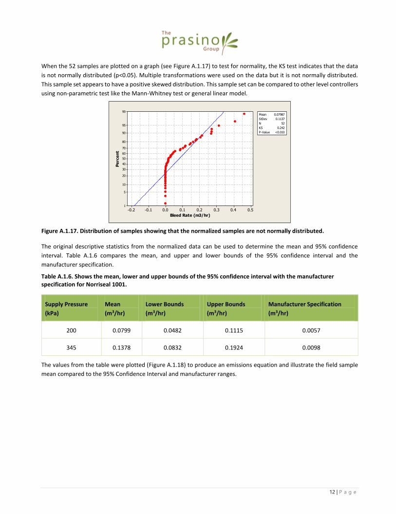
When the 52 samples are plotted on a graph (see Figure A.1.17) to test for normality, the KS test indicates that the data
is not normally distributed (p<0.05). Multiple transformations were used on the data but it is not normally distributed.
This sample set appears to have a positive skewed distribution. This sample set can be compared to other level controllers
using non-parametric test like the Mann-Whitney test or general linear model.
0.50.40.30.20.10.0-0.1-0.2
99
95
90
80
70
60
50
40
30
20
10
5
1
Bleed Rate (m3/hr)
Pe
rce
nt
Mean 0.07987
StDev 0.1137
N 52
KS 0.242
P-Value <0.010
Figure A.1.17. Distribution of samples showing that the normalized samples are not normally distributed.
The original descriptive statistics from the normalized data can be used to determine the mean and 95% confidence
interval. Table A.1.6 compares the mean, and upper and lower bounds of the 95% confidence interval and the
manufacturer specification.
Table A.1.6. Shows the mean, lower and upper bounds of the 95% confidence interval with the manufacturer specification for Norriseal 1001.
Supply Pressure
(kPa)
Mean
(m3/hr)
Lower Bounds
(m3/hr)
Upper Bounds
(m3/hr)
Manufacturer Specification
(m3/hr)
200 0.0799 0.0482 0.1115 0.0057
345 0.1378 0.0832 0.1924 0.0098
The values from the table were plotted (Figure A.1.18) to produce an emissions equation and illustrate the field sample
mean compared to the 95% Confidence Interval and manufacturer ranges.

13 | P a g e
Figure A.1.18. The graph shows the mean and 95% confidence interval and manufacturer specification of gas bled. The bars around the mean represent 50% of the data.
Supply Pressure = 200 kPa Emissions Factor = 0.0799 m3/hr
Supply Pressure = 345 kPa Emissions Factor = 0.1378 m3/hr
Emissions Equation:
Bleed Rate (m3/hr) = 0.0004(Supply Pressure (kPa))
A.1.7 SOR 1530
Thirty one samples were collected for SOR 1530 during sampling. Figure A.1.19 below shows the distribution of samples
normalized for supply pressure.
0.30.20.10.0-0.1
25
20
15
10
5
0
Bleed Rate (m3/hr)
Fre
qu
en
cy
Mean 0.04133
StDev 0.07604
N 31
Figure A.1.19. Distribution of normalized samples.
y = 0.0004x
0
0.05
0.1
0.15
0.2
0.25
0 50 100 150 200 250 300 350 400
Ble
ed R
ate
(m3 /
hr)
Supply Pressure (kPa)
Mean 95% Confidence Interval Manufacturer Specification

14 | P a g e
When the 32 samples are plotted on a graph (see Figure A.1.20) to test for normality, the KS test indicates that the data
is not normally distributed (p<0.05). Multiple transformations were used on the data but it is not normally distributed.
This sample set appears to have a positive skewed distribution. This sample set can be compared to other level controllers
using non-parametric test like the Mann-Whitney test or general linear model.
0.30.20.10.0-0.1-0.2
99
95
90
80
70
60
50
40
30
20
10
5
1
Bleed Rate (m3/hr)
Pe
rce
nt
Mean 0.04133
StDev 0.07604
N 31
KS 0.365
P-Value <0.010
Figure A.1.20. Distribution showing that the normalized samples are not normally distributed.
The original descriptive statistics from the normalized data can be used to determine the mean and 95% confidence
interval. Table A.1.7 compares the mean, and upper and lower bounds of the 95% confidence interval. Manufacturer
maximum steady state air consumption was 0.14 m3/hr at 345 kPa.
Table A.1.7. Shows the mean, lower and upper bounds of the 95% confidence interval for SOR 1530.
Supply Pressure (kPa) Mean (m3/hr) Lower Bounds (m3/hr) Upper Bounds (m3/hr)
200 0.0413 0.0134 0.0692
345 0.0713 0.0232 0.1194
The values from the table were plotted (Figure A.1.21) to produce an emissions equation and illustrate the field sample
mean compared to the 95% Confidence Interval.

15 | P a g e
Figure A.1.21. The graph shows the mean, 95% confidence intervals and manufacturer ranges of gases bled. The bars around the mean represent 50% of the sample points
Supply Pressure = 200 kPa Emissions Factor = 0.0413 m3/hr
Supply Pressure = 345 kPa Emissions Factor = 0.0713 m3/hr
Emissions Equation:
Bleed Rate (m3/hr) = 0.0002(Supply Pressure (kPa))
A.2 Positioner
A.2.1 Fisher Fieldvue 6000
Thirty two samples were collected for Fisher Fieldvue 6000 during sampling. Figure A.2.1 below shows the distribution of
samples normalized for supply pressure using a square root transformation.
0.640.480.320.160.00
7
6
5
4
3
2
1
0
SQRT Bleed Rate (m3/hr)
Fre
qu
en
cy
Mean 0.3265
StDev 0.1843
N 32
Figure A.2.1. Distribution of normalized samples with a square root transformation.
y = 0.0002x
0
0.02
0.04
0.06
0.08
0.1
0.12
0.14
0.16
0 50 100 150 200 250 300 350 400
Ble
ed R
ate
(m3
/hr)
Supply Pressure (kPa)
95% Confidence Interval 95% CI Manufacturer Specification

16 | P a g e
When the 32 samples are plotted on a graph (see Figure A.2.2) to test for normality, the KS test indicates that the data is
normally distributed (p>0.05).
0.80.60.40.20.0
99
95
90
80
70
60
50
40
30
20
10
5
1
SQRT Bleed Rate (m3/hr)
Pe
rce
nt
Mean 0.3265
StDev 0.1843
N 32
KS 0.090
P-Value >0.150
Figure A.2.2. Distribution of samples showing that the normalized samples are normally distributed.
The original descriptive statistics can be used from the normalized data to determine the mean and 95% confidence
interval. Table A.2.1 compares the mean, upper and lower 95% confidence interval and the steady state manufacturer
ranges.
Table A.2.1. Shows the mean, lower and upper bounds of the 95% confidence interval with the manufacturer ranges for Fisher Fieldvue 6000 series.
Supply Pressure
(kPa)
Mean
(m3/hr)
Lower Bounds
(m3/hr)
Upper Bounds
(m3/hr)
Lower Manufacturer
Range (m3/hr)
Upper
Manufacturer
Range (m3/hr)
200 0.1395 0.0950 0.1840 0.0812 0.5801
345 0.2406 0.1639 0.3174 0.1151 0.8757
The values from the table were plotted (Figure A.2.3) to produce an emissions equation and illustrate the field sample
mean compared to the 95% confidence interval and manufacturer ranges.

17 | P a g e
Figure A.2.3. The graph shows the mean, 95% confidence intervals and manufacturer ranges of gases bled. The bars around the mean represent 50% of the sample points.
Supply Pressure = 200 kPa Emissions Factor = 0.1395 m3/hr
Supply Pressure = 345 kPa Emissions Factor = 0.2406 m3/hr
Emissions Equation:
Bleed Rate (m3/hr) = 0.0007(Supply Pressure (kPa))
A.3 Pressure Controller
A.3.2 Fisher 4150
Forty five samples were collected for Fisher 4150 during sampling. Figure A.3.4 below shows the distribution of samples
normalized for supply pressure using a square root transformation.
1.20.90.60.30.0
10
8
6
4
2
0
SQRT (m3/hr)
Fre
qu
en
cy
Mean 0.5206
StDev 0.3317
N 45
Figure A.3.4. Distribution of normalized samples with a square root transformation
y = 0.0007x
0
0.1
0.2
0.3
0.4
0.5
0.6
0.7
0.8
0.9
1
0 50 100 150 200 250 300 350 400
Ble
ed R
ate
(m3
/hr)
Supply Pressure (kPa)
Mean 95% Confidence Interval Manufacturer Range

18 | P a g e
When 45 samples are plotted on graph (see Figure A.3.5) to test for normality, the KS test indicates that the data is
normally distributed (p>0.05). Statistical tests can be used to determine if the Fisher 4150 sample population is
significantly different that other pressure controllers.
1.51.00.50.0
99
95
90
80
70
60
50
40
30
20
10
5
1
SQRT Bleed Rate (m3/hr)
Pe
rce
nt
Mean 0.5206
StDev 0.3317
N 45
KS 0.122
P-Value 0.093
Figure A.3.5. Distribution of samples showing that the normalized samples are normally distributed.
The original descriptive statistics can be used from the normalized data to determine the mean and 95% confidence
interval. Table A.3.2 compares the mean, upper and lower 95% confidence interval and the steady state manufacturer
ranges.
Table A.3.2. Shows the mean, lower and upper bounds of the 95% confidence interval with the manufacturer ranges for Fisher 4150.
Supply Pressure
(kPa)
Mean
(m3/hr)
Lower Bounds (m3/hr) Upper Bounds (m3/hr) Lower
Manufacturer
Range (m3/hr)
Upper
Manufacturer
Range (m3/hr)
200 0.3340 0.2349 0.4445 0.12 0.76
345 0.5864 0.4052 0.7676 0.2 1.2
The values from the table were plotted (Figure A.3.6) to produce an emissions equation and illustrate the field sample
mean compared to the 95% confidence interval and manufacturer ranges.

19 | P a g e
Figure A.3.6. The graph shows the mean, 95% confidence intervals and manufacturer ranges of gases bled. The bars around the mean represent 50% of the sample points.
Supply Pressure = 200 kPa Emissions Factor = 0.3340 m3/hr
Supply Pressure = 345 kPa Emissions Factor = 0.5864 m3/hr
Emissions Equation:
Bleed Rate (m3/hr) = 0.0017(Supply Pressure (kPa))
A.3.3 Fisher 4660
Thirty samples were collected for Fisher 4660 during sampling. Figure A.3.7 below shows the distribution of sample
normalized for supply pressure.
0.200.150.100.050.00-0.05
30
25
20
15
10
5
0
Bleed Rate (m3/hr)
Fre
qu
en
cy
Mean 0.01122
StDev 0.04403
N 30
Figure A.3.7. Distribution of normalized samples.
y = 0.0017x
0
0.2
0.4
0.6
0.8
1
1.2
1.4
0 50 100 150 200 250 300 350 400
Ble
e R
ate
(m3
/hr)
Supply Pressure (kPa)
Mean 95% Confidence Interval Manufactuer Range
20 | P a g e
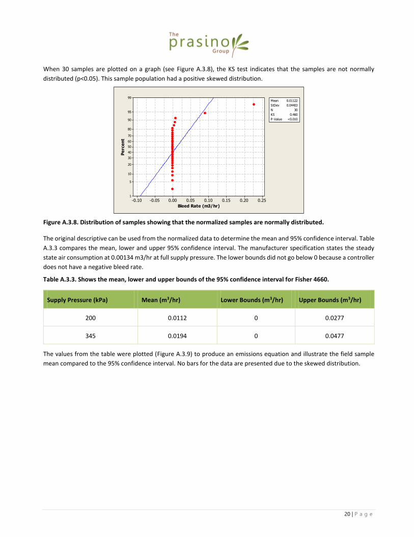
When 30 samples are plotted on a graph (see Figure A.3.8), the KS test indicates that the samples are not normally
distributed (p<0.05). This sample population had a positive skewed distribution.
0.250.200.150.100.050.00-0.05-0.10
99
95
90
80
70
60
50
40
30
20
10
5
1
Bleed Rate (m3/hr)
Pe
rce
nt
Mean 0.01122
StDev 0.04403
N 30
KS 0.460
P-Value <0.010
Figure A.3.8. Distribution of samples showing that the normalized samples are normally distributed.
The original descriptive can be used from the normalized data to determine the mean and 95% confidence interval. Table
A.3.3 compares the mean, lower and upper 95% confidence interval. The manufacturer specification states the steady
state air consumption at 0.00134 m3/hr at full supply pressure. The lower bounds did not go below 0 because a controller
does not have a negative bleed rate.
Table A.3.3. Shows the mean, lower and upper bounds of the 95% confidence interval for Fisher 4660.
Supply Pressure (kPa) Mean (m3/hr) Lower Bounds (m3/hr) Upper Bounds (m3/hr)
200 0.0112 0 0.0277
345 0.0194 0 0.0477
The values from the table were plotted (Figure A.3.9) to produce an emissions equation and illustrate the field sample
mean compared to the 95% confidence interval. No bars for the data are presented due to the skewed distribution.

21 | P a g e
Figure A.3.9. Shows the mean and 95% confidence intervals. Manufacturer specifications are stated above.
Supply Pressure = 200 kPa Emissions Factor = 0.0112 m3/hr
Supply Pressure = 345 kPa Emissions Factor = 0.019351 m3/hr
Emissions Equation:
Bleed Rate (m3/hr) = 0.00006(Supply Pressure (kPa))
A.3.4 Fisher C1
Twenty eight samples were collected for Fisher C1 during sampling. Figure A.3.10 shows the distribution of normalized
samples.
0.40.30.20.10.0-0.1
7
6
5
4
3
2
1
0
SQRT Bleed Rate (m3/hr)
Fre
qu
en
cy
Mean 0.1625
StDev 0.1226
N 28
Figure A.3.10. Distribution of normalized samples.
When 28 samples are plotted on a graph (see Figure A.3.11), the KS test indicates that the samples are normally
distributed using a square root transformation.
y = 6E-05x
0
0.01
0.02
0.03
0.04
0.05
0.06
0 50 100 150 200 250 300 350 400
Ble
ed R
ate
(m3 /
hr)
Supply Pressure (kPa)
Mean (m3/hr) 95% Confidence Interval

22 | P a g e
0.50.40.30.20.10.0-0.1-0.2
99
95
90
80
70
60
50
40
30
20
10
5
1
SQRT Bleed Rate (m3/hr)
Pe
rce
nt
Mean 0.1625
StDev 0.1226
N 28
KS 0.140
P-Value >0.150
Figure A.3.11. Distribution of samples showing the normalized samples are normally distributed.
The original descriptive can be used from the normalized data to determine the mean and 95% confidence interval. Table
A.3.4 compare the mean, lower and upper 95% confidence interval.
Table A.3.4. Shows the mean, lower and upper bounds of the 95% confidence interval for Fisher C1. The manufacturer specification are 0.012 at 241 kPa.
Supply Pressure (kPa) Mean (m3/hr) Lower Bounds (m3/hr) Upper Bounds (m3/hr)
200 0.0409 0.0252 0.0566
345 0.0705 0.0435 0.0976
The values from the table were plotted (Figure A.3.12) to produce and emissions equation and illustrate the field sample
mean compared to the 95% confidence interval.
y = 0.0002x
0
0.02
0.04
0.06
0.08
0.1
0.12
0.14
0 50 100 150 200 250 300 350 400
Ble
ed R
ate
(m3
/hr)
Supply Pressure (kPa)
Mean 95% Confidence Interval Manufacturer Specification

23 | P a g e
Figure A.3.12. The graph shows the men and 95% confidence intervals.
Supply Pressure = 200 kPa Emissions Factor = 0.0409 m3/hr
Supply Pressure = 345 kPa Emissions Factor = 0.0706 m3/hr
Emissions Equation:
Bleed Rate (m3/hr) = 0.0002(Supply Pressure (kPa))
A.4 Temperature Controller
A.4.1 Kimray HT-12
Thirty five samples were collected for Kimray HT12 during field sampling. Figure A.4.1 below shows the distribution of
normalized samples.
0.200.150.100.050.00-0.05
25
20
15
10
5
0
Bleed Rate (m3/hr)
Fre
qu
en
cy
Mean 0.01798
StDev 0.04327
N 35
Figure A.4.1. Distribution of normalized samples.
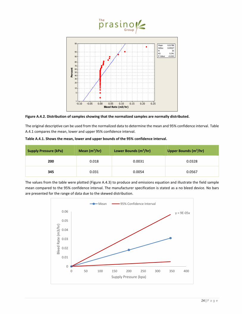
When 35 samples are plotted on a graph (see Figure A.4.2), the KS test indicates that the samples are not normally
distributed. This data shows a positive skewed distribution of samples.
24 | P a g e
0.250.200.150.100.050.00-0.05-0.10
99
95
90
80
70
60
50
40
30
20
10
5
1
Bleed Rate (m3/hr)
Pe
rce
nt
Mean 0.01798
StDev 0.04327
N 35
KS 0.341
P-Value <0.010
Figure A.4.2. Distribution of samples showing that the normalized samples are normally distributed.
The original descriptive can be used from the normalized data to determine the mean and 95% confidence interval. Table
A.4.1 compares the mean, lower and upper 95% confidence interval.
Table A.4.1. Shows the mean, lower and upper bounds of the 95% confidence interval.
Supply Pressure (kPa) Mean (m3/hr) Lower Bounds (m3/hr) Upper Bounds (m3/hr)
200 0.018 0.0031 0.0328
345 0.031 0.0054 0.0567
The values from the table were plotted (Figure A.4.3) to produce and emissions equation and illustrate the field sample
mean compared to the 95% confidence interval. The manufacturer specification is stated as a no bleed device. No bars
are presented for the range of data due to the skewed distribution.
y = 9E-05x
0
0.01
0.02
0.03
0.04
0.05
0.06
0 50 100 150 200 250 300 350 400
Ble
ed R
ate
(m3
/hr)
Supply Pressure (kpa)
Mean 95% Confidence Interval

25 | P a g e
Figure A.4.3. The graph shows the mean and 95% confidence interval. No manufacturer specifications are shown because the Kimray HT12 is a no bleed device with only dynamic bleeding.
Supply Pressure = 200 kPa Emissions Factor = 0.018 m3/hr
Supply Pressure = 345 kPa Emissions Factor = 0.031 m3/hr
Emissions Equations:
Bleed Rate (m3/hr) = 0.00009(Supply Pressure (kPa))
A.5 Transducer
A.5.1 Fairchild TXI 7800 Series
Thirty four samples were collected for Fairchild TXI 7800 series during sampling. Figure A.5.1 below shows the distribution
of normalized samples.
0.60.40.20.0-0.2
8
7
6
5
4
3
2
1
0
Bleed Rate (m3/hr)
Fre
qu
en
cy
Mean 0.2335
StDev 0.1917
N 34
Figure A.5.1. Distribution of normalized samples.
When 34 samples are plotted on a graph (see Figure A.5.2) to test for normality, the KS test indicates that the data is
normally distributed (p>0.05).

26 | P a g e
0.70.60.50.40.30.20.10.0-0.1-0.2
99
95
90
80
70
60
50
40
30
20
10
5
1
Bleed Rate (m3/hr)
Pe
rce
nt
Mean 0.2335
StDev 0.1917
N 34
KS 0.112
P-Value >0.150
Figure A.5.2. Distribution of samples showing that normalized samples are normally distributed.
The descriptive statistics can be used from the normalized data to determine the mean and 95% confidence interval.
Table A.5.1 below compares the mean and 95% confidence interval with the manufacturer specifications.
Table A.5.1. Shows the mean, lower and upper bounds of the 95% confidence interval with the manufacturer ranges for the Fairchild TXI 7800 series.
Supply Pressure (kPa) Mean (m3/hr) Lower
Bounds
(m3/hr)
Upper Bounds
(m3/hr)
Max. Manufacturer Specification
(m3/hr)
200 0.2335 0.1667 0.3004 0.38
345 0.4029 0.2875 0.5183 0.66
The values from the table were plotted (Figure A.5.3) to produce an emissions equation and illustrate the field sample
mean compared to the 95% confidence interval and manufacturer specification.

27 | P a g e
Figure A.5.3. The graph shows the mean, 95% confidence intervals and max manufacturer specification of gases bled. The bars around the mean represent 50% of the sample points.
Supply Pressure = 200 kPa Emissions Factor = 0.2335 m3/hr
Supply Pressure = 345 kPa Emissions Factor = 0.4029 m3/hr
Emissions Factor:
Bleed Rate (m3/hr) = 0.0012(Supply Pressure (kPa))
A.5.2 Fisher 546
Thirty samples were collected for Fisher 546 during sampling. Figure A.5.4 below shows the distribution of samples
normalized for supply pressure.
0.60.40.20.0
7
6
5
4
3
2
1
0
Bleed Rate (m3/hr)
Fre
qu
en
cy
Mean 0.2874
StDev 0.1932
N 30
Figure A.5.4. Distribution of normalized samples.
y = 0.0012x
0
0.1
0.2
0.3
0.4
0.5
0.6
0.7
0 50 100 150 200 250 300 350 400
Ble
ed R
ate
(m3
/hr)
Supply Pressure (kPa)
Mean 95% Confidence Interval Max. Manufacturer Specification

28 | P a g e
When the 30 samples are plotted on a graph (see Figure A.5.4) to test for normality, the KS test indicates that the data is
normally distributed (p>0.05).
0.70.60.50.40.30.20.10.0-0.1-0.2
99
95
90
80
70
60
50
40
30
20
10
5
1
Bleed Rate (m3/hr)
Pe
rce
nt
Mean 0.2874
StDev 0.1932
N 30
KS 0.128
P-Value >0.150
Figure A.5.4. Distribution of samples showing that the normalized samples are normally distributed.
The descriptive statistics can be used from the normalized data to determine the mean and 95% confidence interval and
manufacturer ranges. Table A.5.2 compares the mean, and the upper and lower bounds of the 95% confidence interval.
Table A.5.2. Shows the mean, lower and upper bounds of the 95% confidence interval and manufacturer specification for Fisher 546.
The values from the table were plotted (Figure A.5.5) to produce an emissions equation and illustrate the field sample
mean compared to the 95% confidence interval and manufacturer specification.
Supply Pressure
(kPa)
Mean
(m3/hr)
Lower Bounds
(m3/hr)
Upper Bounds
(m3/hr)
Manufacturer specification
(m3/hr)
200 0.2874 0.2153 0.3596 0.6423
345 0.4958 0.3714 0.6203 1.1080

29 | P a g e
Figure A.5.5. The graph shows the mean, 95% confidence intervals and manufacturer specification of gases bled. The bars around the mean represent 50% of the sample points
Supply Pressure = 200 kPa Emissions Factor = 0.2874 m3/hr
Supply Pressure = 345 kPa Emissions Factor = 0.4029 m3/hr
Emissions Equation:
Bleed Rate (m3/hr) = 0.0014 (Supply Pressure (kPa))
A.5.3 Fisher i2P-100
Thirty six Fisher i2P-100 bleed rate samples were gathered during the field sampling. Figure A.5.6 below shows the
distribution of the corrected field samples.
0.40.30.20.10.0
9
8
7
6
5
4
3
2
1
0
Bleed Rate (m3/hr)
Fre
qu
en
cy
Mean 0.1586
StDev 0.1052
N 36
Figure A.5.6. Distribution of normalized samples.
y = 0.0014x
0
0.2
0.4
0.6
0.8
1
1.2
0 50 100 150 200 250 300 350 400
Ble
ed R
ate
(m3
/hr)
Supply Pressure (kPa)
Mean 95% Confidence Interval Manufacturer Specification

30 | P a g e
Figure A.5.7 plots the normalized data on a graph and the KS P-value indicates that the samples are normally distributed
(p>0.05). On this basis, the average bleed rate can now be compared to other transducers to determine if a generic bleed
rate can be produced or if the populations are significantly different.
0.40.30.20.10.0-0.1
99
95
90
80
70
60
50
40
30
20
10
5
1
Bleed Rate (m3/hr)
Pe
rce
nt
Mean 0.1586
StDev 0.1052
N 36
KS 0.118
P-Value >0.150
Figure A.5.7. A distribution test on the normalized data.
The original descriptive statistics from the normalized data can be used to determine the mean and the 95% confidence
interval. Table compares the mean, and the upper and lower bounds of the 95% confidence interval. The bleed rate
ranges from the manufacturer specification are also provided at both 200 and 345 kPa.
Table A.5.3. Shows the mean and 95% confidence interval compared to the manufacturer specification.
Supply Pressure
(kPa)
Mean
(m3/hr)
Lower Bound
(m3/hr)
Upper Bound
(m3/hr)
Manufacturer Specification
(m3/hr)
200 0.1586 0.1230 0.1942 0.1714
345 0.2736 0.2122 0.3350 0.2957
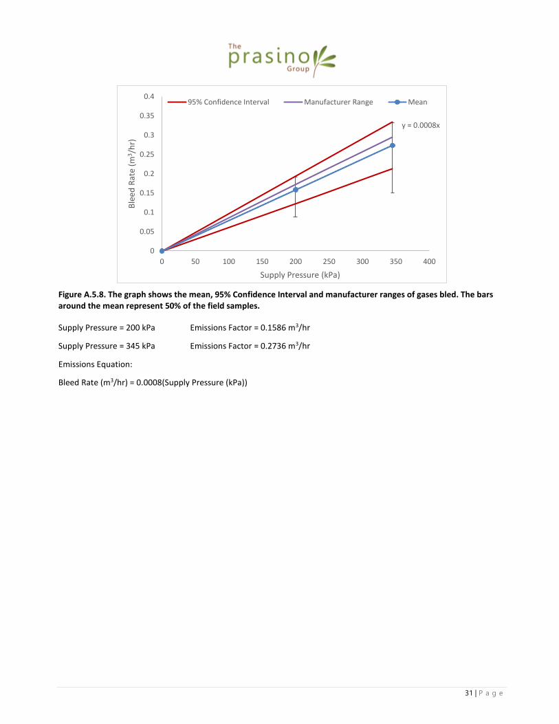
The values from the table were plotted on (Figure A.5.8) an emissions equation and illustrate the field samples mean with
the 95% confidence interval compared to the manufacturer specifications.
31 | P a g e
Figure A.5.8. The graph shows the mean, 95% Confidence Interval and manufacturer ranges of gases bled. The bars around the mean represent 50% of the field samples.
Supply Pressure = 200 kPa Emissions Factor = 0.1586 m3/hr
Supply Pressure = 345 kPa Emissions Factor = 0.2736 m3/hr
Emissions Equation:
Bleed Rate (m3/hr) = 0.0008(Supply Pressure (kPa))
y = 0.0008x
0
0.05
0.1
0.15
0.2
0.25
0.3
0.35
0.4
0 50 100 150 200 250 300 350 400
Ble
ed R
ate
(m3 /
hr)
Supply Pressure (kPa)
95% Confidence Interval Manufacturer Range Mean

32 | P a g e
Appendix B: Normalized Chemical Pump Controller Data
Below is the analysis after a completed sampling program where statistical significant populations were attained for each
pneumatic device included in the survey. A histogram and normality plot were created in Minitab 16. Some of the data
was transformed to determine if the data would need parametric or non-parametric statistical test during the analysis
and report writing phase of the project. A table with standardized operating conditions was used to compare the mean
field bleed rate and 95% confidence interval bands with manufacturer specifications.
B.1 Chemical Injection Pumps
The five chemical injection pumps were normalized for operating conditions including supply pressure and injection rate.
The bleed rate and chemical injection rates were normalized against stokes per minute to develop an emissions factor
based with the independent variable the chemical injection rate and the dependent variable the bleed rate. All pumps
were standardized to 20L/day for initial analysis. However, this will change for the final emissions factor to reflect the
volume of chemical the pump may use.
B.1.1 Morgan HD312
Twenty nine samples were collected for Morgan HD312 Series during sampling. Figure B.1.1 shows the distribution of the
normalized data.
0.200.150.100.050.00
7
6
5
4
3
2
1
0
Normalized Bleed Rate (m3/hr)
Fre
qu
en
cy
Mean 0.07691
StDev 0.05073
N 29
Figure B.1.1. Distribution of normalized samples.
When the 29 samples are plotted on a graph (see Figure B.1.2), the KS test indicates that field sample bleed rates are
normally distributed.

33 | P a g e
0.200.150.100.050.00-0.05
99
95
90
80
70
60
50
40
30
20
10
5
1
Normalized Bleed Rate (m3/hr)
Pe
rce
nt
Mean 0.07691
StDev 0.05073
N 29
KS 0.106
P-Value >0.150
Figure B.1.2. A normality test for normalized field samples.
Figure B.1.3 shows the distribution of chemical injection rates with a log transformation.
1.51.00.50.0-0.5-1.0
7
6
5
4
3
2
1
0
Log Normalized Bleed Rate (m3/hr)
Fre
qu
en
cy
Mean 0.1364
StDev 0.6704
N 29
Figure B.1.3. Distribution for normalized chemical injection rates with a Log transformation.
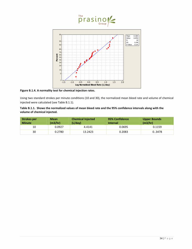
When the 29 samples are plotted on a graph (see Figure B.1.4) to test for normality, the KS test indicates that the chemical
injection rates are normally distributed (p>0.05).
34 | P a g e
2.01.51.00.50.0-0.5-1.0-1.5
99
95
90
80
70
60
50
40
30
20
10
5
1
Log Normalized Bleed Rate (L/day)
Pe
rce
nt
Mean 0.1364
StDev 0.6704
N 29
KS 0.146
P-Value 0.114
Figure B.1.4. A normality test for chemical injection rates.
Using two standard strokes per minute conditions (10 and 30), the normalized mean bleed rate and volume of chemical
injected were calculated (see Table B.1.1).
Table B.1.1. Shows the normalized values of mean bleed rate and the 95% confidence intervals along with the volume of chemical injected.
Strokes per Minute
Mean (m3/hr)
Chemical Injected (L/day)
95% Confidence Interval
Upper Bounds (m3/hr)
10 0.0927 4.4141 0.0695 0.1159
30 0.2780 13.2423 0.2083 0..3478
35 | P a g e
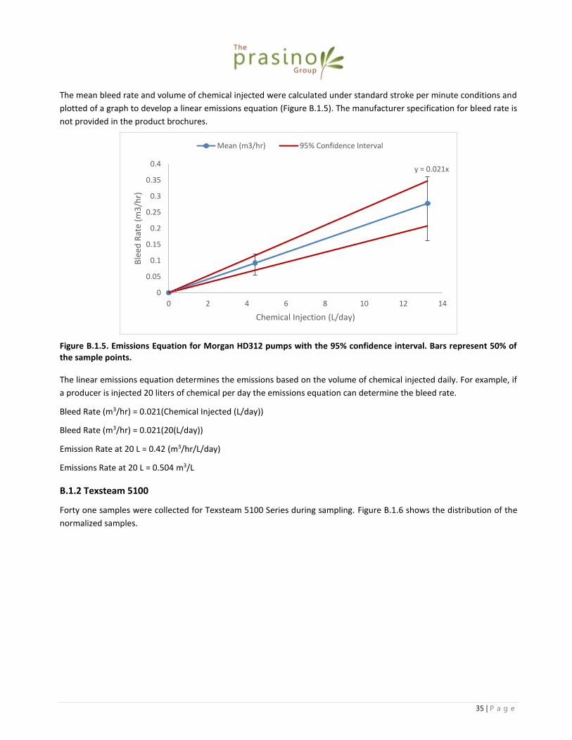
The mean bleed rate and volume of chemical injected were calculated under standard stroke per minute conditions and
plotted of a graph to develop a linear emissions equation (Figure B.1.5). The manufacturer specification for bleed rate is
not provided in the product brochures.
Figure B.1.5. Emissions Equation for Morgan HD312 pumps with the 95% confidence interval. Bars represent 50% of the sample points.
The linear emissions equation determines the emissions based on the volume of chemical injected daily. For example, if
a producer is injected 20 liters of chemical per day the emissions equation can determine the bleed rate.
Bleed Rate (m3/hr) = 0.021(Chemical Injected (L/day))
Bleed Rate (m3/hr) = 0.021(20(L/day))
Emission Rate at 20 L = 0.42 (m3/hr/L/day)
Emissions Rate at 20 L = 0.504 m3/L
B.1.2 Texsteam 5100
Forty one samples were collected for Texsteam 5100 Series during sampling. Figure B.1.6 shows the distribution of the
normalized samples.
y = 0.021x
0
0.05
0.1
0.15
0.2
0.25
0.3
0.35
0.4
0 2 4 6 8 10 12 14
Ble
ed R
ate
(m3
/hr)
Chemical Injection (L/day)
Mean (m3/hr) 95% Confidence Interval

36 | P a g e
0.80.60.40.2
12
10
8
6
4
2
0
Normalized Bleed Rate (m3/hr)
Fre
qu
en
cy
Mean 0.4955
StDev 0.1585
N 41
Figure B.1.6. Distribution of the normalized samples.
When the 44 samples are plotted on a graph (see Figure B.1.7) to test for normality, the KS test indicates that the data is
normally distributed (p> 0.05).
0.90.80.70.60.50.40.30.20.1
99
95
90
80
70
60
50
40
30
20
10
5
1
Normalized Bleed Rate (m3/hr)
Pe
rce
nt
Mean 0.4955
StDev 0.1585
N 41
KS 0.104
P-Value >0.150
Figure B.1.7. A normality test for field samples.
Figure B.1.8 shows the distribution of the normalized chemical injection rates with a square root transformation.

37 | P a g e
87654321
10
8
6
4
2
0
SQRT Normalzied Chemical Injected (L/day)
Fre
qu
en
cy
Mean 4.058
StDev 1.611
N 41
Figure B.1.8. Distribution of Chemical Injected (L/day) with a square root transformation.
When the 41 samples are plotted on a graph (see Figure B.1.9) to test for normality, the KS test indicates that the data is
normally distributed (p> 0.05).
9876543210
99
95
90
80
70
60
50
40
30
20
10
5
1
SQRT Normalized Chemical injected (L/day)
Pe
rce
nt
Mean 4.058
StDev 1.611
N 41
KS 0.093
P-Value >0.150
Figure B.1.9. A normality test for the distribution of chemical injected (L/day).
Using two standard strokes per minute conditions (10 and 30), the normalized mean bleed rate and volume of chemical
injected were calculated (see Table B.1.2).
Table B.1.2. Shows the normalized values of mean bleed rate and the 95% confidence intervals along with the volume of chemical injected.
Strokes Per Minute Mean (m3/hr) Chemical Injected (L/day)
Lower Bounds (m3/hr)
Upper Bounds (m3/hr)
10 0.4955 18.9985 0.4455 0.5455
30 1.4865 56.9955 1.3364 1.6366
38 | P a g e
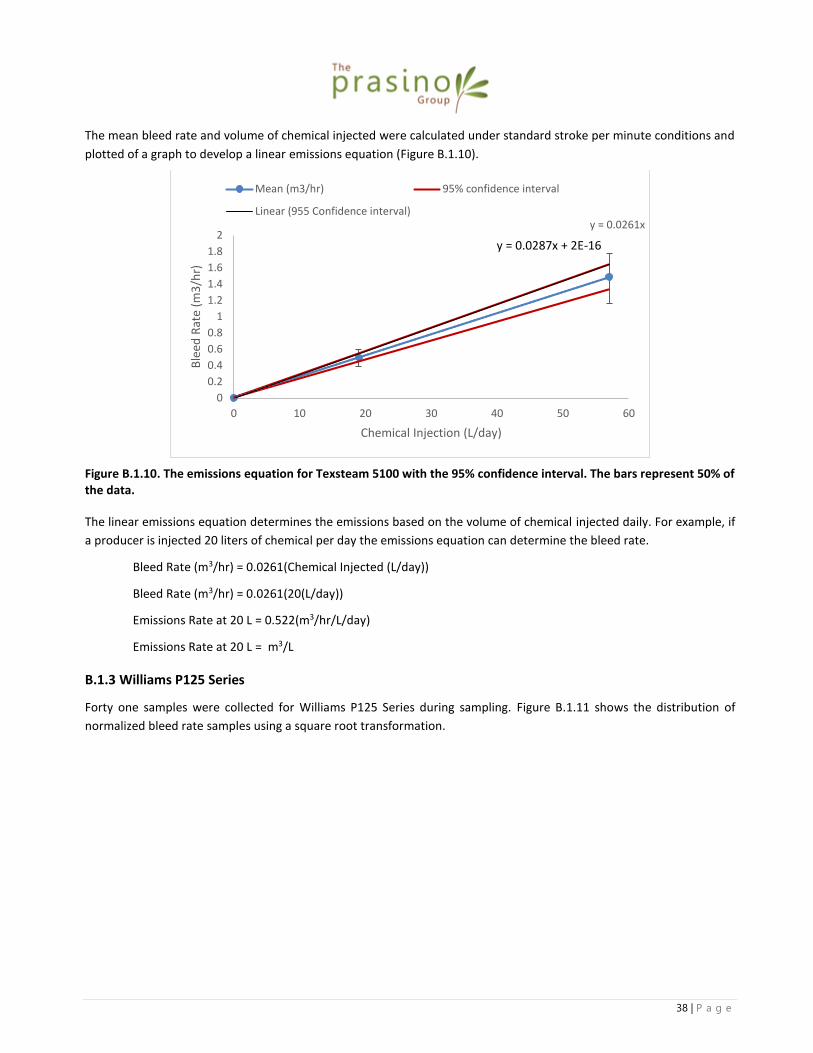
The mean bleed rate and volume of chemical injected were calculated under standard stroke per minute conditions and
plotted of a graph to develop a linear emissions equation (Figure B.1.10).
Figure B.1.10. The emissions equation for Texsteam 5100 with the 95% confidence interval. The bars represent 50% of the data.
The linear emissions equation determines the emissions based on the volume of chemical injected daily. For example, if
a producer is injected 20 liters of chemical per day the emissions equation can determine the bleed rate.
Bleed Rate (m3/hr) = 0.0261(Chemical Injected (L/day))
Bleed Rate (m3/hr) = 0.0261(20(L/day))
Emissions Rate at 20 L = 0.522(m3/hr/L/day)
Emissions Rate at 20 L = m3/L
B.1.3 Williams P125 Series
Forty one samples were collected for Williams P125 Series during sampling. Figure B.1.11 shows the distribution of
normalized bleed rate samples using a square root transformation.
y = 0.0261x
y = 0.0287x + 2E-16
0
0.2
0.4
0.6
0.8
1
1.2
1.4
1.6
1.8
2
0 10 20 30 40 50 60
Ble
ed R
ate
(m3
/hr)
Chemical Injection (L/day)
Mean (m3/hr) 95% confidence interval
Linear (955 Confidence interval)

39 | P a g e
Figure B.1.11. Distribution of normalized bleed rate samples showing a positive skewed distribution.
When the 41 samples are plotted on the graph (see Figure B.1.12) to test for normality, the KS test indicates the data is
not normally distributed (p<0.05). Statistical test can still be used to compare Williams pumps, due to the robustness of
data and the use of different statistical tests.
Figure B.1.12. A normality test for the distribution of normalized samples using a square root transformation.
Figure B.1.13 shows the distribution of normalized chemical injection rates using a square root transformation.
0.800.640.480.320.160.00
14
12
10
8
6
4
2
0
SQRT SP/SPM
Fre
qu
en
cy
Mean 0.3294
StDev 0.1942
N 41
0.80.60.40.20.0
99
95
90
80
70
60
50
40
30
20
10
5
1
SQRT SP/SPM
Pe
rce
nt
Mean 0.3294
StDev 0.1942
N 41
KS 0.212
P-Value <0.010

40 | P a g e
Figure B.1.13. Distribution of normalized chemical injection rates using a square root transformation.
When the 41 samples were plotted on graph (see Figure B.1.14) to test for normality, the KS test indicates that the data
is normally distributed (p>0.05).
Figure B.1.14. A normality test for the distribution of normalized chemical injected rates.
Using two standard strokes per minutes conditions (10 and 30), the normalized bleed rate and chemical injection rate
were calculated (see Table B.1.).
Table B.1.3. Shows the normalized values of mean bleed rate and 95% confidence interval along with volume of chemical injected.
Strokes Per Minute Mean (m3/hr) Chemical Injected (L/day)
Lower Bounds (m3/hr) Upper Bounds (m3/hr)
10 0.1751 8.5005 0.1108 0.2394
30 0.5253 25.5016 0.3324 0.7181
6.04.83.62.41.20.0
9
8
7
6
5
4
3
2
1
0
SQRT Chemical Injected
Fre
qu
en
cy
Mean 2.554
StDev 1.425
N 41
6543210-1
99
95
90
80
70
60
50
40
30
20
10
5
1
SQRT CI/SPM
Pe
rce
nt
Mean 2.554
StDev 1.425
N 41
KS 0.138
P-Value 0.048

41 | P a g e
The mean bleed rate and volume of chemical injected were calculated under standard stroke per minute conditions and
plotted of a graph to develop a linear emissions equation (Figure B.1.15).
Figure B.1.15. The emissions equation for Williams P125 Series with the 95% confidence interval. The bars represent 50% of the data.
Bleed Rate (m3/hr) = 0.0206(Chemical Injected (L/day))
Bleed Rate (m3/hr) = 0.0.206(20(5) L/day)
Emissions Rate at 20L/day = 0.412 (m3/hr/L/day)
Emissions Rate at 20L/day = 0.4944 m3/L
B.1.4 Williams P250 Series
Forty one samples were collected for Williams P125 Series during sampling. Figure B.1.16 shows the distribution of
normalized bleed rate samples using a square root transformation.
y = 0.0206x
0
0.1
0.2
0.3
0.4
0.5
0.6
0.7
0.8
0 5 10 15 20 25 30
Ble
ed R
ate
(m3
/hr)
Chemical Injected (L/day)
Mean 95% Confidence Interval

42 | P a g e
Figure B.1.16. The distribution of normalized samples.
When 21 samples are plotted on the graph (see Figure B.1.17) to test for normality, the KS test indicates that the data is
normally distributed (p>0.05). Statistical test can be used to compare different sized Williams pumps.
Figure B.1.17. A normality test for the distribution of normalized samples.
Figure B.1.18 shows the normalized distribution of chemical injection rates.
0.350.300.250.200.150.100.05
9
8
7
6
5
4
3
2
1
0
Normalized Bleed Rate (m3/hr)
Fre
qu
en
cy
Mean 0.1494
StDev 0.05568
N 21
0.350.300.250.200.150.100.050.00
99
95
90
80
70
60
50
40
30
20
10
5
1
Normalized Bleed Rate (m3/hr)
Pe
rce
nt
Mean 0.1494
StDev 0.05568
N 21
KS 0.183
P-Value 0.066

43 | P a g e
Figure B.1.18. Distribution of normalized chemical injection samples.
When the 21 samples are plotted on the graph (see Figure B.1.19) to test for normality, the KS test indicates that the data
is normally distributed (p>0.05).
Figure B.1.19. A normality test for the distribution of normalized chemical injection rates.
Using two standard stroke conditions, the normalized bleed rate and chemical injection rates were calculated.
Table B.1.4. Shows the normalized values of mean bleed rate and 95% confidence interval along with volume of chemical injected.
Strokes per Minute Mean (m3/hr) Chemical Injected (L/day)
Lower Bounds (m3/hr) Upper Bounds (m3/hr)
10 0.1427 4.0566 0.1147 0.1706
30 0.4285 12.1698 0.3446 0.5125
7654321
4
3
2
1
0
Normalized Chemical Injected (L/day)
Fre
qu
en
cy
Mean 3.992
StDev 1.516
N 21
876543210
99
95
90
80
70
60
50
40
30
20
10
5
1
Normalized Chemical Injected (L/day)
Pe
rce
nt
Mean 3.992
StDev 1.516
N 21
KS 0.122
P-Value >0.150

44 | P a g e
The mean bleed rate and volume of chemical injected were calculated under standard stroke per minute conditions and
plotted of a graph to develop a linear emissions equation (Figure B.1.20).
Figure B.1.20. The emissions equation for Williams P250 Series with the 95% confidence interval. The bars represent 50% of the data.
Bleed Rate (m3/hr) = 0.0352(Chemical Injection (L/day)
Bleed Rate (m3/hr) = 0.0352 (20 L/day)
Emissions Rate at 20L = 0.704 (m3/hr/L/day)
Emissions Rate at 20L = 0.8448 m3/L
B.1.5 Williams P500 Series
Twelve samples were collected for Williams P500 Series during sampling. Figure B.1.21 shows the distribution of samples.
0.70.60.50.40.30.20.1-0.0
5
4
3
2
1
0
Normalized Bleed Rate (m3/hr)
Fre
qu
en
cy
Mean 0.3720
StDev 0.1569
N 12
Figure B.1.21. Distribution of normalized sample bleed rates.
y = 0.0352x
-0.1
0
0.1
0.2
0.3
0.4
0.5
0.6
0 2 4 6 8 10 12 14
Ble
ed R
ate
(m3
/hr)
Chemical Injected (L/day)
Mean (m3/hr) 95% Confidence Interval

45 | P a g e
When the 12 samples are plotted on the graph (see Figure B.1.22) to test for normality, the KS test indicates that the data
is normally distributed (p>0.05).
0.80.70.60.50.40.30.20.10.0
99
95
90
80
70
60
50
40
30
20
10
5
1
Normalized Bleed Rate (m3/hr)
Pe
rce
nt
Mean 0.3720
StDev 0.1569
N 12
KS 0.145
P-Value >0.150
Figure B.1.22. A normality test for the distribution of normalized bleed rates.
Figure B.1.23 shows the distribution of normalized chemical injection rates.
16012080400-40
4
3
2
1
0
Normalized Chemical Injected (L/day)
Fre
qu
en
cy
Mean 47.75
StDev 49.19
N 12
Figure B.1.23. A normality test for the distribution of normalized samples.
When the 12 samples are plotted on the graph (see Figure B.1.24) to test for normality, the KS test indicates that the data
is normally distributed.

46 | P a g e
Figure B.1.24. A normality test for the distribution of normalized chemical injection rates
Using two standard stroke rates conditions, the normalized bleed rate and chemical injection rates were calculated.
Table B.1.5. Shows the normalized values of mean bleed rate and 95% confidence interval along with volume of chemical injected.
Strokes per Minute Mean (m3/hr) Chemical Injected (L/day)
Lower Bounds (m3/hr) Upper Bounds (m3/hr)
10 0.3720 47.7478 0.2723 0.4717
30 1.1160 143.2433 0.8168 1.4150
The mean bleed rate and volume of chemical injected were calculated under standard stroke per minute conditions and
plotted of a graph to develop a linear emissions equation (Figure B.1.25).
150100500-50-100
99
95
90
80
70
60
50
40
30
20
10
5
1
Normalized Chemical Injected (m3/hr)
Pe
rce
nt
Mean 47.75
StDev 49.19
N 12
KS 0.204
P-Value >0.150

47 | P a g e
Figure B.1.25. The emissions equation for Williams P500 Series with the 95% confidence interval. The bars represent 50% of the data.
Bleed Rate (m3/hr) = 0.0078(Chemical Injection (L/day))
Bleed Rate (m3/hr) = 0.0078 (20 L/day)
Bleed Rate at 20L = 0.156 (m3/hr)
Emissions Rate at 20L = 0.1872 (m3/L)
y = 0.0078x
0
0.2
0.4
0.6
0.8
1
1.2
1.4
1.6
0 20 40 60 80 100 120 140 160
Ble
ed R
ate
(m3
/hr)
Chemical Injected (L/day)
Mean Lower Bounds (95%CI)