1  

Supporting Information for Nanoscale deformation in polymers revealed by single-molecule super-resolution localization-orientation microscopy Muzhou Wang,1,2 James M. Marr,3,4 Marcelo Davanco,3 Jeffrey W. Gilman,1 J. Alexander Liddle3 1Department of Chemical and Biological Engineering, Northwestern University, Evanston, IL 60208 2Materials Measurement Laboratory, National Institute of Standards and Technology, Gaithersburg, MD 20899 3Center for Nanoscale Science and Technology, National Institute of Standards and Technology, Gaithersburg, MD 20899 4Maryland NanoCenter, University of Maryland, College Park, MD 20742 Determining Localization Uncertainty

Figure S1. a) Super-resolution images of 1:1 lines and spaces of 100 nm and 40 nm pitch, written by electron-beam lithography in a 40 nm thick PMMA film. These images are compared to scanning electron micrographs of the same features. b) Integrated intensity from super-resolution images along the lines over a 3 µm × 3 µm area. Experimental data is compared to expected profiles that account for localization precision derived from the root-mean-squared CRLB, σprec = 4.0 nm (blue dotted), and total uncertainty that includes both precision and accuracy (green solid), σ = 8.2 nm. c) Line-space contrast vs. pitch of the features, summarized in a modulation transfer function (MTF). Contrast is defined as the ratio of the difference between the bright and dark intensities vs. the sum, averaged over the many line-space periods in the integrated area. Error bars based on the periods are not shown because they are smaller than the drawn points. Experimental data is compared to simulated data, with the same color scheme as in (b). Note that the x-axis is reversed, with high values on the left.

To measure the accuracy of the estimated single-molecule positions, we take advantage of the fact that PMMA is an excellent high-resolution electron-beam resist. Lithographically-patterned nanoscale features are a natural choice for a ground truth test structure. For our features, we chose

Electronic Supplementary Material (ESI) for Materials Horizons.This journal is © The Royal Society of Chemistry 2019

2  

1:1 lines and spaces of varying pitch, which we confirmed using top-down scanning electron microscopy (SEM). These are easily resolved down to 40 nm pitch in the super-resolution images, which can be matched against the SEM images (Fig. S1a). We integrate the images along the lines to generate well-sampled, low-noise data for comparison with expected intensity profiles, which in this case are 1:1 square waves convolved with a Gaussian of variance σ2 equal to the localization uncertainty (Fig. S1b). If we use the root-mean-squared localization precision of 4.0 nm as σ, the resulting profile does not fit the data well. This precision corresponds to the Cramer-Rao lower bound (CRLB) variance estimating the fluorophore positions as determined using maximum likelihood estimation (MLE), and arises from the limited photon counts from each single molecule. Instead, we find that σ = 8.2 nm provides an excellent fit for all the feature sizes we examined. This suggests that the total localization uncertainty contains contributions from both the CRLB precision, along with imperfect localization accuracy, where the localized position of each fluorophore is displaced slightly from its true position. The line-space contrast at all pitches can be summarized in a modulation transfer function (Fig. S1c).

Since errors add quadratically, 2 2i , the remaining non-CRLB localization uncertainty

is 7.2 nm. This additional error may arise from many sources including imperfect index-matching, slight defocus due to the finite film thickness, imprecise drift correction methods,1 field-dependent aberrations such as coma and field curvature,2 overlapping PSFs,3 etc. These factors are difficult to quantify and are the subject of ongoing work. Nevertheless, the overall localization uncertainty of 8.2 nm is sufficiently small to reveal important nanoscale phenomena. Image Fitting

Expected point-spread functions. Our analysis of the orientation-based point-spread functions (PSFs) closely follows the work of Mortensen, et al.4,5 and will be briefly reproduced here, mostly focusing on the discussion of image fitting. Full derivations of the optical principles underlying the PSFs can be found in the associated references, and thus the PSFs are shown here without proof.

For a fluorophore with orientations given by an azimuthal angle α and polar angle β (90° is perpendicular to the optical axis), its PSF is given by,

2 2

2 2

cos 2 2 sin sin cos cos cos,

sin cos

P P P PF x y

I I

. (1)

More specifically, this PSF is a normalized probability density function for the probability of finding a photon in the camera plane at a position (x, y) relative to the fluorophore’s true location. This relative position is magnification-corrected to more conveniently correspond to the lengths at the sample focal plane rather than the camera plane, and is expressed in polar coordinates (ρ, ϕ) in the PSF definition. The radius-dependent P functions in (1) are defined as,

* *14

*

*

*12

Im

Re

P AA BB

P CC

P B A C

P AB

, (2)

where * denotes complex conjugate. A, B, and C are all functions of ρ defined as,

3  

max

max

max

0

0

2

0

1

0

cos

cos

cos

p s

p s

p

A E E J k M d

B E E J k M d

C E J k M d

, (3)

where k = 2π/λ from the emission wavelength, M is the magnification of the objective, and Jn are nth order Bessel functions of the 1st kind. The I constants in (1) are defined as,

max

max

* *14

0

2 2

2 20

*

0

2

2 20

2

2 cos

2

2

cos

p s p s

p

I AA BB d

E E E E dk M

I CC d

E dk M

, (4)

where the simplifications are made possible by the closure relation of Bessel functions,

0

n n

u vJ ux J vx xdx

u

. (5)

The ηʹ variable denotes an angle with the optical axis of a propagating light wave in air, while η is this angle in the sample, and thus these two variables are related by Abbe’s sine condition,

sin sinn M , (6)

where n is the refractive index of the sample. The functions sE , pE , and pE are s- and p-polarized

components of the far-field plane waves that radiate from a dipole either parallel or perpendicular to the sample plane. In the case examined throughout this work of a fluorophore in an index-matched medium, these functions are especially simple,

cos

sin

s

p

p

E nk

E nk

E nk

. (7)

The plane waves within the angles accepted by the numerical aperture of the objective are those that determine the PSF. Thus, in the functions A, B, and C, the upper limits of integration are given by,

max maxsin sinNA n M , (8)

where NA is the numerical aperture. In practice, the radiation pattern from a fluorophore is projected onto a camera with pixels of

size Δx, and thus it is important to determine the number of photons that is expected to land on each pixel. We will work in a coordinate system such that the position (xi, yi) of the ith pixel is

4  

defined relative to a fixed point (such as the center of a region of interest). If a fluorophore is located at a point (x0, y0), then the value of the normalized PSF at each pixel is given by,

0 0,i i iF F x x y y . (9)

Note that the polar coordinates of each pixel can be determined using the common definitions, 0 cosi i ix x , 0 sini i iy y . (10)

If the fluorophore emits N photons, then a simple approximation for the expected number of photons in a given pixel is given by,

2i iNF b x , (11)

where b is a constant number of photons per unit area, arising from background sources. However, this is potentially a poor approximation as it does not account for how the shape and curvature of the radiation patterns can vary within a single pixel. A better approximation is to integrate F(x, y) after using a Taylor expansion,

2

2

2 2

2

2

/2 /2

0 0

/2 /2

21/2 /22

2

21/2 /2 2

2 124

,

...

i i

i i

i i

i i

x x y x

i

x x y x

F F Fx x y x i i i ix yi xi i

F Fx x y x i i ix yy ii

Fi x

NF x x y y b dydx

F x x y y x xN dydx b x

y y x x y y

NF b x N

2

2 2

4 6Fy i

x O x

. (12)

This provides an expression for the expected number of photons in each pixel for a fluorophore emitting N photons, located at a position (x0, y0), with azimuthal angle α and polar angle β.

Fitting an experimental image. In an experiment, our task is to determine N, x0, y0, α, and β from an image of the fluorophore. The expected number of photons in the ith pixel of this image is simply μi(N, x0, y0, α, β, b) as given in (12). A real image is typically acquired as a set of values Di that correspond to the number of ADU counts in each pixel, which can be converted by the camera offset and gain to give the number of photons in each pixel,

ioffset / gaini i im D , (13)

where the gain is units of ADU counts per photons. All cameras also add a contribution from readout noise to the signal, which can be measured as a variance in the ADU count reading in perfectly dark conditions. This variance can be gain-corrected,

2var / gaini i iv , (14)

to be given in units of photons. Note that our experiments used an EMCCD camera so these parameters are well-approximated as pixel-independent, but we show the more general calculations for those who may use sCMOS detector where the parameters can vary significantly for different pixels.6 In both cases, these values must be characterized prior to the experiment and are treated as known quantities here. The quantity mi + vi is a random variable that is well-described by a Poisson distribution,

1

1i i i

q vi i i i i

i

P q m v v eq

, (15)

capturing shot noise effects. For convenience, we introduce variables for the readout noise-corrected photon counts,

5  

i i im m v , i i iv , (16)

and thus (15) becomes,

1

1i iq

i i ii

P q m eq

(17)

Given data from the fluorophore image mi, the six parameters that determine μi can be determined by maximum likelihood estimation (MLE). The overall likelihood function for a given set of parameters is given by,

0 0

1, , , , ,

1

log log

i imi

i i

ii i i

i i

L N x y b em

L m mm

. (18)

This function is then maximized using a Newton-Raphson method with respect to a vector describing the six parameters,

1 2 3 4 5 6 0 0, , , , , , , , , ,N x y b θ . (19)

To do this, we begin with a suitably chosen initial guess θ0, and then iterate according to the relation,

1

1 log logn n L L

θ θθ θ H , (20)

where and H are the gradient vector and Hessian matrix of the log-likelihood function with respect to the six parameters, and –1 denotes a matrix inverse. The components are given by,

22

2

loglog 1

loglog 1

i ij

i ij j i

i i i i ijk

i ij k j k i j k i

mLL

m mLL

θ

θH

. (21)

When successive parameter values are close enough within a tolerance, the algorithm then terminates. Note that for convergence, the Hessian matrix must be negative definite throughout the iteration. In certain steps this condition is not always satisfied, in which case an eigenvalue decomposition is performed on H, and an identity matrix multiplied by the largest eigenvalue is subtracted from H to guarantee convergence. Additionally, successive steps are taken through a series of checks to ensure that the parameters do not vary too quickly. Finally, this algorithm is easily adapted to handle multiple fluorophores within one region of interest,3 by simply including additional parameters describing more emitters in the maximization. For Nem emitters, the number of parameters in the vector θ is given by 5Nem + 1.

The endpoint of this iterative algorithm is a set of parameters θ, that maximize the likelihood function (18), and is thus the best possible estimate for the brightness, position, and orientation of a fluorophore as given by its image.

To determine the precision of our estimates, we calculate the Fisher information matrix,

log log

jkj k

L LI E

, (22)

where E denotes an expectation value. In our case, it can be easily shown from (18) that this expression can be simplified to become,

6  

1 i i

jki i j k

I

, (23)

which is evaluated at the parameters θ that maximize the likelihood. The Cramer-Rao lower bound precision for estimating each parameter is determined by inverting this matrix, C = I–1. The j, kth element of C is the covariance of θj and θk. For example, the precision of our estimate for α is C44, because θ4 is α.

Implementation. The fitting scheme as described above was implemented in MATLAB using home-built codes, which are included in this publication. First, the functions P in (2) and constants I in (4) are integrated numerically. The functions P are stored as a list of evaluated constants at finely-spaced ρ values, and the constants I are stored directly. This data must only be calculated once for a given optical situation (such as sample refractive index, numerical aperture, emission wavelength, etc.) and can thus be stored as a library and loaded. The camera constants in (13) and (14) are also determined and stored. After applying a commonly available image segmentation routine, regions of interest containing possible fluorophores are then fed as inputs mi into a subroutine that executes the MLE scheme shown in (20).

The challenge in each iteration step is evaluating the various derivatives that determine the gradient vector and Hessian matrix (21), which can be calculated analytically from the definitions of the PSF. We do not include an exhaustive list of these derivatives here for brevity, but a few are shown for demonstration,

2 2

2 2

3 3

3 2

3 3

2 2

2 4 4

2 4 2 2

2 4124

2 4124

0

2 4124

2

2

2

22 41

2420

2

0

0

i F Fi x y i

i F F Fx i x x y i

i F F Fi x y i

i

i

i F F Fx x x yi i

i

F x xN

N x N xx

N x N x

xb

N

N x N xx

Ny

2 4 4

2 3

2 4124

F F Fy x y yi i

x N x

. (24)

It is apparent that many of these derivatives involve calculating derivatives of the PSF. Derivatives with respect to angles can be evaluated directly from the definition (1), for example,

7  

2

2 2

2 sin 2 2 sin sin cos sin

sin cos

P PF F

I I

. (25)

Derivatives with respect to position are more conveniently evaluated using the operators in polar coordinates,

1

cos sinF F F

x r

, 1

sin cosF F F

y r

. (26)

The derivatives with respect to ρ require derivatives of the P functions, which are also pre-calculated and stored in the library. For example,

max

max

**

1

0

20 2

0

cos

2cos

p

p

P C CC C

CE J k M d

J k M J k MkM E d

. (27)

To sample the P derivatives from the library, the polar coordinates of each pixel (ρi, ϕi) are determined at each iteration step, and the value of the P derivative is determined by linear interpolation from ρi. Additionally, polar coordinates are also determined for the positions halfway between each pixel, and the function values there are useful for calculating position derivatives using finite difference.

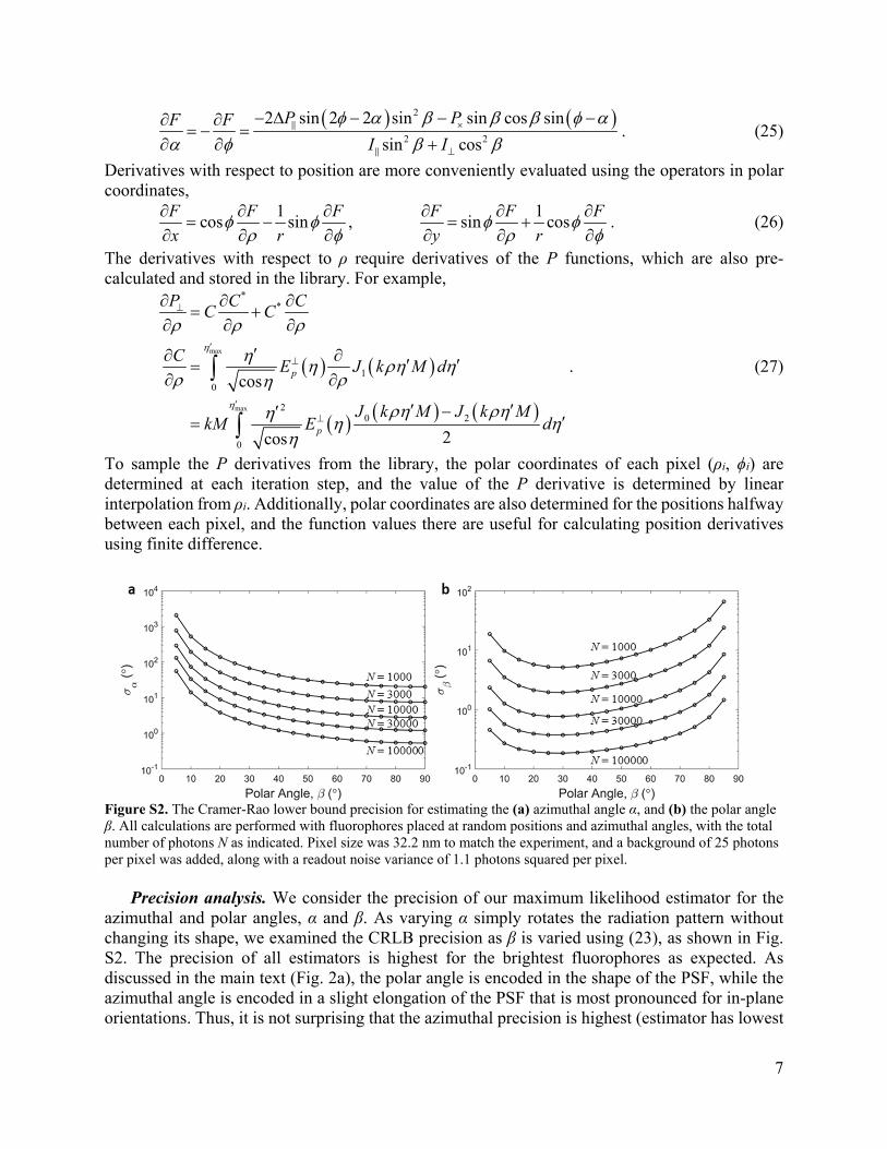
Figure S2. The Cramer-Rao lower bound precision for estimating the (a) azimuthal angle α, and (b) the polar angle β. All calculations are performed with fluorophores placed at random positions and azimuthal angles, with the total number of photons N as indicated. Pixel size was 32.2 nm to match the experiment, and a background of 25 photons per pixel was added, along with a readout noise variance of 1.1 photons squared per pixel.

Precision analysis. We consider the precision of our maximum likelihood estimator for the

azimuthal and polar angles, α and β. As varying α simply rotates the radiation pattern without changing its shape, we examined the CRLB precision as β is varied using (23), as shown in Fig. S2. The precision of all estimators is highest for the brightest fluorophores as expected. As discussed in the main text (Fig. 2a), the polar angle is encoded in the shape of the PSF, while the azimuthal angle is encoded in a slight elongation of the PSF that is most pronounced for in-plane orientations. Thus, it is not surprising that the azimuthal precision is highest (estimator has lowest

8  

variance) when β is large, since those images provide the highest information content. The polar precision is best in the middle of the β range, because the PSF has the least sensitivity to β when β is close to 0° or 90°. For example, differences between the bottom two PSFs in Fig. 2a are difficult to discern by eye.

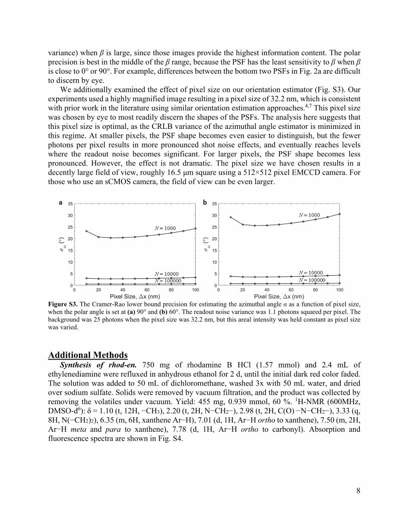
We additionally examined the effect of pixel size on our orientation estimator (Fig. S3). Our experiments used a highly magnified image resulting in a pixel size of 32.2 nm, which is consistent with prior work in the literature using similar orientation estimation approaches.4,7 This pixel size was chosen by eye to most readily discern the shapes of the PSFs. The analysis here suggests that this pixel size is optimal, as the CRLB variance of the azimuthal angle estimator is minimized in this regime. At smaller pixels, the PSF shape becomes even easier to distinguish, but the fewer photons per pixel results in more pronounced shot noise effects, and eventually reaches levels where the readout noise becomes significant. For larger pixels, the PSF shape becomes less pronounced. However, the effect is not dramatic. The pixel size we have chosen results in a decently large field of view, roughly 16.5 μm square using a 512×512 pixel EMCCD camera. For those who use an sCMOS camera, the field of view can be even larger.

Figure S3. The Cramer-Rao lower bound precision for estimating the azimuthal angle α as a function of pixel size, when the polar angle is set at (a) 90° and (b) 60°. The readout noise variance was 1.1 photons squared per pixel. The background was 25 photons when the pixel size was 32.2 nm, but this areal intensity was held constant as pixel size was varied. Additional Methods

Synthesis of rhod-en. 750 mg of rhodamine B HCl (1.57 mmol) and 2.4 mL of ethylenediamine were refluxed in anhydrous ethanol for 2 d, until the initial dark red color faded. The solution was added to 50 mL of dichloromethane, washed 3x with 50 mL water, and dried over sodium sulfate. Solids were removed by vacuum filtration, and the product was collected by removing the volatiles under vacuum. Yield: 455 mg, 0.939 mmol, 60 %. 1H-NMR (600MHz, DMSO-d6): δ = 1.10 (t, 12H, −CH3), 2.20 (t, 2H, N−CH2−), 2.98 (t, 2H, C(O) −N−CH2−), 3.33 (q, 8H, N(−CH2)2), 6.35 (m, 6H, xanthene Ar−H), 7.01 (d, 1H, Ar−H ortho to xanthene), 7.50 (m, 2H, Ar−H meta and para to xanthene), 7.78 (d, 1H, Ar−H ortho to carbonyl). Absorption and fluorescence spectra are shown in Fig. S4.

9  

Figure S4. Absorption and emission spectra of rhod-en in ethanol. Absorption of the initial non-fluorescent form is shown in black. The transition to the bright state can be induced by acid in addition to ultraviolet light. After adding 1% of 36% hydrochloric acid, the solution turned bright red, and the absorption and emission spectra of this form are shown in green and red. λmax, abs = 553 nm, λmax, em = 578 nm. Absorption spectra are normalized to the maximum of the bright state.

Synthesis of rhod-butyl. 130 mg of rhodamine B HCl (0.271 mmol) and 1 mL of butylamine

were refluxed in 5 mL of anhydrous ethanol for 2 d, until the initial dark red color faded. The solution was added to 50 mL of dichloromethane, washed 3x with 50 mL water, and dried over sodium sulfate. Solids were removed by vacuum filtration, and the product was collected by removing the volatiles under vacuum. Yield: 104 mg, 0.209 mmol, 77 %. 1H-NMR (600 MHz, DMSO-d6): δ = 0.62 (t, 3H, −CH3), 0.99 (m, 4H C−CH2−CH2−C), 1.09 (t, 12H, N−C−CH3), 2.96 (t, 2H, C(O)−N−CH2−), 3.33 (q, 8H, N(−CH2)2), 6.34 (m, 6H, xanthene Ar−H), 7.05 (d, 1H, Ar−H ortho to xanthene), 7.51 (m, 2H, Ar−H meta and para to xanthene), 7.77 (d, 1H, Ar−H ortho to carbonyl).

Synthesis of PMMA-D. The bright and dark forms of rhodamine spirolactam dye have an acid-base equilibrium, so the polymer was modified with basic monomers to optimize this equilibrium. Methyl methacrylate (MMA) was distilled over calcium hydride under vacuum. N,N-dimethylaminoethyl methacrylate (DMAEMA) was passed through basic alumina. Azobisisobutyronitrile (AIBN) was recrystallized from methanol. A solution of 2.00 g of MMA (20.0 mmol), 20 µL of DMAEMA (0.12 μmol), and 1.00 mg of AIBN (6.1 μmol) in 8.0 mL of anisole was degassed and heated to 70 °C and stirred under nitrogen overnight. The viscous solution was diluted in anisole and precipitated in hexane, and the resulting polymer was dried under vacuum. Molar mass distribution was determined on a gel permeation chromatography system with a refractive index detector. The mobile phase was tetrahydrofuran, and the sample was separated at 1 mL/min through three Waters Styragel HR columns connected in series. Against PMMA standards, the molar mass of the synthesized polymer was Mn = 170 kg/mol and Mw = 477 kg/mol. Yield: 1.30 g, 65 %. 1H-NMR (600MHz, CDCl3): δ = 0.85-1.05 (m, 3H, backbone −CH3), 1.8-2 (m, 2H, backbone −CH2−), 2.94 (s, 0.03H, N−CH3), 3.62 (s, 3H, O−CH3).

Single-molecule imaging apparatus. Single-molecule imaging was performed on an inverted microscope, summarized in Fig. S5. Visible illumination was achieved by passing a 532 nm continuous wave laser at 300 mW through a cleanup bandpass filter (FWHM bandwidth 2.0 nm), a spatial filter and lenses for cleanup and magnification, a half-wave plate and polarizer to adjust

10  

intensity, and a quarter-wave plate. A 355 nm Q-switched laser at 4 mW average power was passed through similar optics. The orientation of the waveplates were adjusted to achieve circular polarization at the sample. Both beams were combined using a dichroic mirror (414 nm edge wavelength) and focused onto the back aperture of a 150X, NA = 1.45, oil immersion objective. The intensity of the 532 nm illumination was held at 6 kW/cm2 to 7 kW/cm2 at the sample, while the 355 nm illumination was adjusted throughout the experiment to a maximum of 60 mW/cm2. Fluorescence emission was spectrally filtered using a dichroic mirror (538 nm edge wavelength) and a bandpass filter (579 nm center wavelength, FWHM bandwidth 43.5 nm). Single-molecule images at the camera port were magnified using relay lenses (focal lengths 60 mm and 200 mm) onto an electron-multiplying charge-coupled device camera. The effective pixel size of the detector was 32.2 nm in sample dimensions, and acquisitions were performed at a gain of 25 and a frame speed of 2 Hz. 72,000 frames were collected for each super-resolution image shown in this study.

To achieve near-ideal imaging conditions, various sources of error were systematically eliminated. Lateral drift was mitigated using fiducial markers and finding fluorophore positions relative to the markers as fixed references. To introduce the markers, a slurry of 100 nm diameter nanodiamonds in isopropanol containing green fluorescent nitrogen vacancy centers (Adamas Nanotechnologies)† was sonicated and drop-cast onto each sample prior to imaging. Axial drift was mitigated using a home-built focus lock system, which introduced a 785 nm laser into the objective at a high angle to achieve total internal reflection, and then collected the reflected laser beam onto a complementary metal-oxide semiconductor (CMOS) camera. Axial motions as small as 1 nm could be detected from deflections in the laser beam, and these were compensated using a piezo-controlled sample stage. Aberrations from the air-polymer interface were removed by applying a drop of glycerol onto the sample, whose refractive index of 1.473 closely matches 1.491 of the polymer and 1.515 of the glass.

Figure S5. Schematic of single-molecule imaging setup.

11  

Electron-beam lithography. No. 1 glass coverslips were heated in Piranha solution (3:1 sulfuric acid to 30 % aqueous hydrogen peroxide) at 100 °C overnight. Caution: this is a highly corrosive and oxidizing solution and should be handled with extreme care. A solution of mass fraction 0.5 % rhod-en relative to PMMA-D was spin-coated from anisole onto the coverslips and baked at 180 °C for 5 min. The polymer film thickness was 40 nm as verified by reflectometry on films spun-coat on silicon wafers under identical conditions. 10 nm of aluminum was deposited onto the polymer by thermal evaporation at < 10−3 Pa (10−5 Torr). Line-and-space patterns of varying pitch were then written onto the sample using an electron beam lithography system, with an accelerating voltage of 100 kV, spot size 2 nm, and beam current of 0.5 nA. Optimal areal doses were determined to be 1.4 mCcm-2 to 1.6 mCcm-2. After exposure, the aluminum layer was removed using 0.26 mol/L tetramethylammonium hydroxide in water, and the features were developed by soaking the coverslips with light agitation in a solution of 1:3 water to isopropanol at 0 °C for 4 min.8 After sputtering 1 nm of AuPd alloy onto the polymer film, the features were imaged by scanning electron microscopy at a 2 kV accelerating voltage. Identical samples without the AuPd coating were then imaged by single-molecule microscopy.

Optical simulations. To determine whether the small refractive index difference between the PMMA and above glycerol layer produced any significant bias in the observed PSFs, we performed finite-difference time-domain (FDTD) simulations to model a single molecule emitting within the fabricated nanostructure. In these simulations, a single electric point dipole was placed within the protrusion 70 nm above the polymer-glass interface (Fig. S9), and oriented in either the x, y or z direction. The refractive indices for the various media are listed above, and their spatial distribution used for the FDTD simulation was obtained from the AFM data, which was assumed to give a faithful description of the PMMA nanostructure topography above a 10 nm residual PMMA film at the bottom of the wells. The steady-state electromagnetic field produced by the point dipole at =580 nm was recorded at a plane parallel to the glass slide surface, located 10 nm below the polymer-glass interface. This steady-state near-field was then used to calculate the radiated (vector) far-field as a function of the azimuthal and polar angles.9

The far-field plane waves were used to determine the image intensity using the analysis of Richards and Wolf,10 and applied by several other authors.4,11,12 This was also used in the vectorial diffraction calculations for determining PSFs for comparison with experimental images to determine fluorophore orientation throughout this study. Assuming that the light propagating in the –z direction is collected to form an image, the far-field plane waves were first decomposed into

,sE and ,pE , which represent s- and p-polarized contributions parallel to unit vectors,

ˆ ˆ ˆsin cos

ˆ ˆ ˆ ˆcos cos sin cos sins

p

e x y

e x y z

, (28)

where ψ and η are the azimuthal and polar angles in glass. This plane wave propagates in the direction parallel to ˆ ˆp se e .The electric field at the image plane is then given by,

max 2

cos

0 0

ˆ ˆ, , ,cos

ikp p s sE e e E e E d d

, (29)

where k = 2π/λ, (r, θ) are polar coordinates at the image plane, and ηʹ is the polar angle in air. This angle is related to the polar angle in glass by Abbe’s sine condition (6), and the upper limit of integration is related to the numerical aperture (8). The electric field integral also depends on the s- and p-polarized unit vectors in air. The s-polarization is the same as Eq. 1, and the p-polarized unit vector in air is given by,

12  

ˆ ˆ ˆ ˆcos cos sin cos sinpe x y z . (30)

After evaluating the E-field using (29), we then calculate the light intensity distribution at the image plane,

* *, x x y yI r E E E E . (31) †Disclaimer: Certain commercial equipment, instruments, or materials are identified in this

report in order to specify the experimental procedure adequately. Such identification is not intended to imply recommendation or endorsement by the National Institute of Standards and Technology, nor is it intended to imply that the materials or equipment identified are necessarily the best available for the purpose. Additional Figures

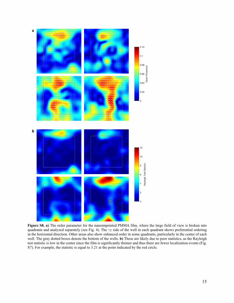
To explore how the alignment phenomenon varied over the many wells in the large field of view of the experiment, we divided the large area into quadrants and performed an identical analysis within each region. The +y side contained regions of enhanced orientational order in every quadrant, confirming that the orientation effect is consistent over all the wells (Fig. S8). The effect of slightly imperfect index matching was also explored through finite-difference time-domain simulations of an oscillating dipole placed in the protrusion of the fabricated nanostructure (Figs. S9 and S10). PSFs using the experimental material configurations of glycerol on PMMA on glass are essentially indistinguishable from simulations and the analytical diffraction calculations that assume perfect index matching. The simulations also showed that minimal effect on the PSF arises when single molecules are defocused by 70 nm, which is the largest difference in sample thickness within the deformed regions. The many controls shown here confirm that the observed orientational alignment does not originate from experimental or imaging artifacts, and arises definitively from the mechanical deformation introduced during the nanofabrication process.

Below are some figures relevant to the nanoimprinting experiment.

13  

Figure S6. Rendered super-resolution image of total analyzed area for nanoimprint experiment (see Fig. 4a). There were roughly 105 events over an area of 7 µm × 7 µm. Scale bar is 500 nm.

14  

Figure S7. Event density in the combined nanoimprinted wells, after applying the Gaussian kernel of σ = 15 nm. To calculate the Rayleigh test statistic (Eq. 4) at a given location, the number of events in the rendered angular distribution n is equal to 2πσ2 times the event density shown here. The gray dotted box denotes the bottom of the well, where inside the box the film is 10 nm thick and outside it is 70 nm thick.

15  

Figure S8. a) The order parameter for the nanoimprinted PMMA film, where the large field of view is broken into quadrants and analyzed separately (see Fig. 4). The +y side of the well in each quadrant shows preferential ordering in the horizontal direction. Other areas also show enhanced order in some quadrants, particularly in the center of each well. The gray dotted boxes denote the bottom of the wells. b) These are likely due to poor statistics, as the Rayleigh test statistic is low in the center since the film is significantly thinner and thus there are fewer localization events (Fig. S7). For example, the statistic is equal to 3.21 at the point indicated by the red circle.

16  

Figure S9. a) PMMA nanostructure topography used for the FDTD simulation. The red X indicates the location of the electric point dipole. b) y = 0 and c) x = 0 plane cross sections of the refractive index distribution. The glycerol index matching fluid is denoted by IMF.

Figure S10. Comparison of point-spread functions for an oscillating dipole emitting at 580 nm, oriented along the 3 axes. The length of one side of each image is 600 nm. The first column shows results from a finite-difference time-domain (FDTD) simulation using the experimental dielectric materials geometry of glycerol above PMMA above glass, with the dipole placed in the protrusion, 70 nm above the plane of the coverslip. In the second column, the top material is assigned to n = 1.491 to exactly match the PMMA. The third column shows analytical PSFs that were used for fitting experimental images throughout this study. The fourth column shows analytical PSFs defocused at 70 nm. Intensity differences between the PSFs are less than 0.5% everywhere, with no detectable rotational bias.

17  

References (1) Dai, M.; Jungmann, R.; Yin, P. Optical Imaging of Individual Biomolecules in Densely

Packed Clusters. Nat. Nanotechnol. 2016, 11 (9), 798–807. (2) Diezmann, A. Von; Lee, M. Y.; Lew, M. D.; Moerner, W. E. Correcting Field-Dependent

Aberrations with Nanoscale Accuracy in Three-Dimensional Single-Molecule Localization Microscopy. Optica 2015, 2 (11), 985.

(3) Huang, F.; Schwartz, S. L.; Byars, J. M.; Lidke, K. A. Simultaneous Multiple-Emitter Fitting for Single Molecule Super-Resolution Imaging. Biomed. Opt. Express 2011, 2, 1377–1393.

(4) Mortensen, K. I.; Churchman, L. S.; Spudich, J. A.; Flyvbjerg, H. Optimized Localization Analysis for Single-Molecule Tracking and Super-Resolution Microscopy. Nat. Methods 2010, 7 (5), 377–381.

(5) Mortensen, K. Optimized Data Analysis for Localization-Based Microscopy, Technical University of Denmark, 2010.

(6) Huang, F.; Hartwich, T. M. P.; Rivera-Molina, F. E.; Lin, Y.; Duim, W. C.; Long, J. J.; Uchil, P. D.; Myers, J. R.; Baird, M. a; Mothes, W.; et al. Video-Rate Nanoscopy Using SCMOS Camera-Specific Single-Molecule Localization Algorithms. Nat. Methods 2013, 10 (7), 653–658.

(7) Mortensen, K. I.; Sung, J.; Flyvbjerg, H.; Spudich, J. A. Optimized Measurements of Separations and Angles between Intra-Molecular Fluorescent Markers. Nat. Commun. 2015, 8621.

(8) Rooks, M. J.; Kratschmer, E.; Viswanathan, R.; Katine, J.; Fontana, R. E.; MacDonald, S. A. Low Stress Development of Poly(Methylmethacrylate) for High Aspect Ratio Structures. J. Vac. Sci. Technol. B 2002, 20 (6), 2937–2941.

(9) Taflove, A.; Hagness, S. C. Computational Electrodynamics: The Finite-Difference Time-Domain Method, 3rd ed.; Artech House: Norwood, MA, 2005.

(10) Richards, B.; Wolf, E. Electromagnetic Diffraction in Optical Systems. II. Structure of the Image Field in an Aplanatic System. Proc. R. Soc. A Math. Phys. Eng. Sci. 1959, 253 (1274), 358–379.

(11) Böhmer, M.; Enderlein, J. Orientation Imaging of Single Molecules by Wide-Field Epifluorescence Microscopy. J. Opt. Soc. Am. B 2003, 20, 554–559.

(12) Backlund, M. P.; Lew, M. D.; Backer, a. S.; Sahl, S. J.; Grover, G.; Agrawal, A.; Piestun, R.; Moerner, W. E. Simultaneous, Accurate Measurement of the 3D Position and Orientation of Single Molecules. Proc. Natl. Acad. Sci. 2012, 109 (47), 19087–19092.