Marshall UniversityMarshall Digital Scholar

Theses, Dissertations and Capstones

1-1-2010

Determining the Rate of Transcription of T7 RNAPolymerase Using Single Molecule FluorescenceImagingDawn Renee Nicholadawn0623@gmail.com

Follow this and additional works at: http://mds.marshall.edu/etdPart of the Biochemistry Commons

This Thesis is brought to you for free and open access by Marshall Digital Scholar. It has been accepted for inclusion in Theses, Dissertations andCapstones by an authorized administrator of Marshall Digital Scholar. For more information, please contact zhangj@marshall.edu.

Recommended CitationNichola, Dawn Renee, "Determining the Rate of Transcription of T7 RNA Polymerase Using Single Molecule Fluorescence Imaging"(2010). Theses, Dissertations and Capstones. Paper 112.

DETERMINING THE RATE OF TRANSCRIPTION OF T7 RNA POLYMERASE USING SINGLE MOLECULE

FLUORESCENCE IMAGING

A Thesis submitted to The Graduate College of

Marshall University

In partial fulfillment of The requirements for the degree of

Master of Science

Chemistry

by Dawn Renee Nicholas

Approved by

Dr. Michael Norton, Ph.D., Committee Chairperson Dr. Leslie Frost, Ph.D.

Dr. Brian Scott Day, Ph.D.

Marshall University December 2010

ii

Acknowledgments

I would like to thank everyone who has helped me complete this project. First I

would like to thank my husband, Jesse Nicholas. You have been very supportive and

willing to help me out whenever I need it. I would also like to thank my parents, Robert

and Rebecca Stump, and my brother, Tony Stump. All of you have supported me since

grade school. Without your love and support this would not have been possible.

I would also like to express my thanks to my advisor, Dr. Michael Norton.

You’ve given me the opportunity to learn new techniques while I was working in the lab,

and you’ve always been there to answer questions. You have helped to guide me through

my capstone and thesis project. Thank you. I would also like to thank everyone in the

Norton lab group both present (Masudur Rahman, David Neff, Nathaniel Crow,

Samantha Cotsmire, Melanie Butt, Van Hoang, Anshuman Mangalum, and Wallace

Kunin) and past members that I have worked with. Everyone has always been helpful to

talk to and ask questions. I especially want to thank Wallace for helping me with the

Matlab code and David for helping to explain the microscopes to me. Everyone has been

fun to work with, and I will miss all of you.

My thanks also go to my committee members, Dr. Leslie Frost and Dr. Brian S.

Day. Thank you for your insights and support. Last, I would like to thank the Marshall

Chemistry Department. Thank you to everyone; the classes, advice, and support have

been greatly appreciated.

iii

Table of Contents

Title...................................................................................................................................... i

Acknowledgments ............................................................................................................. ii

Table of Contents ............................................................................................................. iii

List of Figures .....................................................................................................................v

List of Tables .................................................................................................................. viii

Abstract ............................................................................................................................. ix

Introduction

RNA and Transcription in Cells ...........................................................................1

T7 RNA Polymerase ..............................................................................................3

Rolling Circle Transcription .................................................................................5

Single Molecule Fluorescence Imaging ................................................................6

Overview of Project ...............................................................................................9

Determination of Transcription Rate.................................................................11

Experimental

Microscope Setup .................................................................................................15

Circularization of DNA .......................................................................................18

In vitro Rolling Circle Transcription .................................................................19

Cleaning Glass and Flow Cell Construction ......................................................20

Photostability of Cy3 Labeled DNA ...................................................................22

Single Molecule Fluorescence Imaging of Transcription .................................23

BSA Coated Flow Cell .........................................................................................23

Poly-L-lysine Coated Flow Cell ..........................................................................24

Results and Discussion

Circularization of DNA .......................................................................................24

In vitro Rolling Circle Transcription .................................................................28

Photostability of Cy3 labeled DNA .....................................................................30

iv

Single Molecule Fluorescence Imaging of Transcription .................................35

BSA Coated Flow Cell .........................................................................................46

Poly-L-lysine Coated Flow Cell ..........................................................................48

Single Molecule Fluorescence with Poly-L-lysine coated Flow Cell ................48

Control Experiment .............................................................................................52

Fourier Transform ...............................................................................................53

Conclusions .......................................................................................................................55

Appendix

Appendix A- 45nt DNA Circle ............................................................................57

Appendix B- Secondary Structure of 45nt DNA Circle ...................................58

Appendix C- Ethanol Precipitation Protocol ....................................................59

Appendix D- Summary of SpotSelect Script .....................................................60

Appendix E- SpotSelect Code .............................................................................73

References .........................................................................................................................82

v

List of Figures

Figure 1: The four nucleic acid bases that make up RNA1…………………………. 1

Figure 2: Representation of the conformation of T7 RNA polymerase during

initiation (top) and elongation (bottom) …………..………………………………… 3

Figure 3: Picture of a microscope set up to use TIRF. The prism directs the light

from the laser to the surface at an angle that can create the evanescent wave needed

for TIRF.23

…………………………………………………………………………… 8

Figure 4: Cy3 molecule/ pseudobase that is inserted into the DNA strand. The image

is from idtdna.com …………………..………………………………………………. 10

Figure 5: Picture of fluorescence microscope used in the single molecule

experiments ………………………………………………………………………….. 16

Figure 6: Hg lamp spectra. There is a large peak at 546 nm that corresponds well

with Cy3.22

………………………………...…………………………………………. 16

Figure 7: Excitation and emission spectra of Cy3 using Spectra Viewer from

Invitrogen.com. The dashed line is the excitation and the solid line is the emission.

The grayed areas are the filter sets that are used for the Cy3 ……………..……… 17

Figure 8: (Top) Image of CCD camera used to detect the fluorescence of the single

Cy3 molecules. ………………………………………………………………………. 18

Figure 9: Cartoon construction of the two types of flow cells. (Left) The first where

the glass coverslip is attached to the slide with double sided tape and the other two

ends are sealed with epoxy. (Right) The flow cell where the glass coverslip is

attached to the slide with the double sided tape and the other two ends are left open

to allow liquid to be wicked through…………………………………………………. 21

Figure 10: (Top) UV-Vis spectra of linear ssDNA with Cy3 inserted into the

phosphate backbone. (Bottom) UV-Vis spectra of circular ssDNA with Cy3 inserted

into the phosphate backbone ………………………...………………………………. 25

Figure 11: 15% polyacrylamide gel stained with ethidium bromide. Lane A contains

the 45nt linear ssDNA, lane B contains the DNA after the Circligase reaction, lane

C contains the 45nt circular DNA, and lane D contains the Ultra low range DNA

ladder …….................................................................................................................... 26

Figure 12: UV-Vis spectra of purified RNA in 1x TE buffer. Transcription was

performed using the circular ssDNA with the Cy3 internal modification as the

template……………………………………………………………………………… 28

vi

Figure 13: 1.2% FlashGel with RNA Millennium Marker (Lane A), control reaction

(Lane B), transcription reaction after incubation at 37°C (Lane C), and purified

concentrated RNA from transcription (Lane D)………………..……………………. 28

Figure 14: Fluorescence image of RNA annealed with short rhodamine labeled

DNA and combed onto a clean glass surface ………………………………………. 29

Figure 15: Fluorescence image of Cy3 labeled DNA in transcription buffer. This

image is the 1st frame of a 500 frame movie ……………….…..………………….. 31

Figure 16: Two graphs showing the intensity over time (seconds) of a Cy3 labeled

DNA in transcription buffer. Both graphs show one-step photobleaching that shows

that there was only one molecule producing the light …..………………….. 32

Figure 17: Graphs showing the number of fluorescent molecules active after a given

time in a movie. These data points were fit to an exponential curve. The top graph

shows the number of molecules active at varying times for the Cy3 labeled DNA

dried on a glass coverslip, the bottom left graph shows the number of molecules

active at varying times for the Cy3 labeled DNA in water, and the bottom right

graph shows the number of molecules active at varying times for the Cy3 labeled

DNA in 1x transcription buffer .................................................................................... 34

Figure 18: Image of a clean glass flow cell loaded with 2.5mM NTP mix. Many

fluorescent spots from the NTP mix can be seen in this sample …………….…….. 36

Figure 19: Image of clean glass flow cell with 0.5x transcription buffer, 2.5mM

NTPs, 1mM DTT, and 0.01mM Trolox. No fluorescence was seen in this image… 36

Figure 20: Background corrected 1st frame of a 750 frame movie. The fluorescent

spots are the Cy3 labeled DNA imaged during transcription with T7 RNAP in

2.5mM NTP mix …………………………………………………………………….. 37

Figure 21: (A) Wiener filtered intensity data from Spot 44 from the transcription of

the Cy3 labeled DNA with a concentration of 2.5mM NTP mix. (B) Unfiltered

intensity data for the same spot in A..……………………………………………….. 37

Figure 22: (A) Graph of the intensity over time of Wiener filtered spot in

transcription with 2.5mM NTP concentration. (B) Graph of the intensity over time

of Wiener filtered spot in transcription with a 0.125mM NTP concentration ……… 41

vii

Figure 23: Histograms of the time between the peaks for all of the spots selected at

each concentration of NTP. (A) 5mM NTP concentration (B) 2.5mM NTP

concentration (C) 1.25mM NTP concentration (D) 0.75mM NTP concentration (E)

0.5mM NTP concentration (F) 0.25mM NTP concentration (G) 0.125mM NTP

concentration ............................................................................................................... 45

Figure 24: (A) Fluorescent Optosplit image of BSA coated flowcell rinsed with UV-

treated PEM-80 buffer. (B) Fluorescent Optosplit image of BSA coated flow cell

rinsed with 0.5x transcription buffer with 0.5mM NTP, 1mM DTT, and 0.01mM

Trolox ……………………………………………………………………………… 47

Figure 25: Fluorescent Optosplit image of poly-L-lysine coated flow cell ……… 47

Figure 26: Background corrected 1st frame of transcription of Cy3 labeled DNA in

poly-L-lysine coated flow cell with 0.5mM NTP concentration ……………………. 49

Figure 27: Graph of background and illuminant corrected, Wiener filtered intensity

data of spot 25 in the movie of transcription in a poly-L-lysine coated flow cell with

0.5mM NTP concentration …...……………………………………………………… 48

Figure 28: Histograms of the times between the peaks of the modulations in the

movies of transcription in poly-L-lysine coated flow cells at various concentrations.

(A) 0.5mM NTP (B) 0.25mM NTP (C) 0.125mM NTP …….………………………. 52

Figure 29: Background corrected 1st frame of negative control for transcription

experiment …………………………………………………………………………… 52

Figure 30: Graph of the intensity of the Cy3 labeled DNA in transcription buffer

with T7 RNAP, DTT, and Trolox ……………………..……………………………. 54

Figure 31: Power spectrum of Wiener filtered intensity data ……………..………… 54

Figure 32: Power spectrum of Wiener filtered intensity data with DC component

removed……………………………………………………………………………… 55

viii

List of Tables

Table 1: Different transcription rates and the techniques used to calculated

them for T7 RNAP…………………..………………………..………………. 12

Table 2: The photochemical half-life of the Cy3 labeled DNA dried on glass,

in water, and in 1x transcription buffer ………………………..………………. 35

Table 3: Table of the average time between peaks of the modulations in the

intensity data of the Cy3 labeled DNA during transcription with different

concentrations of NTPs. The transcription rate of the T7 RNAP was calculated

from the average time between the peaks ……………………………………… 39

Table 4: List of time between peaks of modulations and the corresponding

transcription rate for transcription with three different NTP concentrations … 41

Table 5: Average time between peaks of modulations and the corresponding

transcription rate for poly-L-lysine coated flow cell at different NTP

concentrations ………………………………………………………………….. 50

ix

Abstract

It is important to understand the many factors impacting the rate at which an RNA

polymerase incorporates nucleotides. The transcription rate of T7 RNA polymerase has

been determined using single molecule fluorescence microscopy. A Cy3 labeled circular

45nt ssDNA molecule was used to monitor the transcription process. T7 RNA

polymerase was used because it is a single subunit polymerase that does not need any

cofactors and will transcribe single-stranded DNA circles that do not contain a promoter.

The transcription was monitored by measuring the quasi-periodic change in

intensity associated with the transit of the probe through the polymerase as the DNA is

transcribed. The time between these intensity changes of the Cy3 molecule represents the

time it takes the polymerase to transcribe the circle once. Transcription rates were

determined at a variety of NTP concentrations. Because glass can affect how the enzyme

works, the surface of the glass was coated with poly-L-lysine in some of the experiments.

The poly-L-lysine was used to keep the T7 RNAP from touching the glass surface. In

order to extend the observation time, factors affecting the photostability of the Cy3 probe

were evaluated using determinations of the photochemical half-life.

1

Introduction

RNA and Transcription in Cells

In cells, transcription is a biological process in which complementary RNA

(ribonucleic acid) is made from genomic DNA

via an enzyme called an RNA polymerase.

RNA is made up of four main bases: adenine,

cytosine, guanine, and uracil. Figure 1 shows

the structure of the 4 nucleic acid bases in

RNA.(1)

Each of these bases is connected to a

ribose sugar that is attached to a phosphate

group that comprises the backbone of the

RNA. The RNA will base pair with another

complementary RNA strand. Each base has a

complement and will pair through two or three hydrogen bonds. Adenine pairs with uracil

and cytosine pairs with guanine. These base pairings create double stranded RNA or

DNA:RNA hybrids. During transcription the growing RNA chain forms a DNA:RNA

hybrid in the polymerase. The RNA base complementary to the base in the template

DNA is added to the growing RNA polymer. This is how the DNA passes along the

information it carries.

There are three main types of cellular RNA: messenger RNA, ribosomal RNA,

and transfer RNA. Each of these three RNA types has different size and secondary

characteristics that help with its specific jobs.(2) The messenger RNA comprises about

5% of the RNA in a cell. Messenger RNA is the most heterogenous type of RNA in

Figure 1: The four nucleic acid bases that

make up RNA.(1)

2

regard to size and sequence. This RNA carries information from the DNA and is used as

the template for protein synthesis. The messenger RNA travels from the nucleus where it

was synthesized into the protein synthesis sites in the cytosol.(2)

The ribosomal RNA forms part of the ribosomes that are responsible for

synthesizing proteins. Ribosomal RNA accounts for about 80% of the RNA in a cell. In

eukaryotic cells there are four species of ribosomal RNA, and in the prokaryotic cells

there are three species of ribosomal RNA. These differences in the number and size of the

ribosomal RNA account for the difference in structure of the ribosome in eukaryotic and

prokaryotic cells.(2)

The last type of RNA is the transfer RNA. Transfer RNA are the smallest of the

three types of RNA. There is a different type of tRNA for each of the twenty amino acids.

The transfer RNA carries its amino acid to the ribosome where it adds the amino acid

according to the messenger RNA code. The transfer RNA contains unusual bases such as

N4-Acetylcytosine. The unusual bases help the RNA be recognized by specific enzymes

and to keep it from being digested by RNases. The secondary and tertiary structure of the

transfer RNA is important to its ability to carry its specific amino acid.(2)

In a cell, transcription is closely regulated by proteins. The proteins guide the

polymerase to where transcription should occur. There is usually a specific sequence

called a promoter region immediately before the sequence that needs to be transcribed.

The promoter region signals to the polymerase that it needs to bind to it and start

transcribing. Transcription can be divided into three distinct sections: initiation,

elongation, and termination. In initiation, the polymerase binds to the DNA and starts

making short pieces of RNA, usually less than 10 bases long. Elongation occurs when the

3

polymerase releases the promoter and starts sliding along the DNA making the

complementary RNA. Termination occurs when the polymerase releases the RNA it was

making and the DNA it was bound to.

T7 RNA Polymerase

The RNA polymerase that we used was T7 RNA polymerase (RNAP). T7 RNAP

is from the T7 bacteriaphage virus. This polymerase is a single subunit enzyme that is

only about 100kDa(3)

compared to RNA polymerase II from yeast that consists of 12

subunits and is 500kDa(4)

. T7 RNAP is one

of the most studied RNA polymerases due

to its relative simplicity and has been used

in many rolling circle transcription

studies.(5)(6)(7)(8)

Numerous crystal

structures in various stages have also been

made and are in the protein data bank.(9)

During the initiation stage, the

RNAP loosely binds to the DNA template

strand. The RNAP starts to transcribe the

template strand. The RNAP undergoes

abortive synthesis in which it transcribes

many short (8-12 nt) RNA strands before

the RNAP starts the second stage of

transcription, elongation. While the short RNA strands are being made, the RNAP

Figure 2: Representation of the conformation

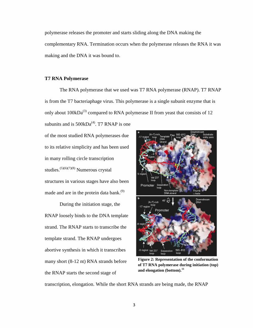
of T7 RNA polymerase during initiation (top)

and elongation (bottom).11

4

remains bound to the promoter region and does not move along the DNA strand, which is

why the RNA that is made is less than 12nt long.(10)

Once the T7 RNAP has transcribed 8-10 nucleotides and released the promoter, if

there is one, the elongation stage has started. During this stage the RNAP can produce

RNA over 15,000 nucleotides in length. During this stage the elongation process is very

stable. To obtain this stability the T7 RNAP undergoes a conformational change. The N-

terminal end of the protein (residues 2-266) reorients to form three structural entities.

Residues 2-71form an N-terminal extension, residues 152-205 form a central flap, and

residues 258-266 form a C-terminal linker that connects the N-terminal and C-

terminal.(11)

Figure 2 (top) shows the T7 RNAP in the initiation conformation. Figure 2

(bottom) shows the T7 RNAP in the elongation conformation. In the elongation

conformation, the polymerase folds around the DNA making a pocket where transcription

occurs. The template strand goes through the pocket, is transcribed, and is part of a

DNA:RNA hybrid for 10-12 bases. The non-template strand goes around the outside of

the RNA polymerase and binds with the template strand after the RNA has been

separated from the DNA.(11)

The number of nucleotides the polymerase attaches to the RNA strand per second

is called the transcription rate. Numerous studies have been performed to determine the

transcription rate of polymerases, and these techniques will be discussed in the next

section. Determining the transcription rate can be difficult due to pausing. Pausing occurs

when the RNAP temporarily stops transcribing during elongation. Different polymerases

pause for different periods of time. T7 RNAP pauses less often and for a shorter period of

5

time than some other RNA polymerases, which makes it a good RNA polymerase to use

for this study.(12)

The last stage of transcription is termination. Termination occurs when the

polymerase releases the RNA it was transcribing and the template DNA. For T7 RNAP

the termination is sequence dependent. A sequence in the template DNA causes the RNA

to form a hairpin that destabilizes the structure. Usually there are multiple uracil bases in

the RNA before termination. The uracils destabilize the RNA:DNA hybrid inside of the

polymerase.(13)

Rolling Circle Transcription

RNA transcription is the cellular process in which complementary RNA is made

from DNA through the use of an enzyme called an RNA polymerase. Rolling circle

transcription (RCT) is a special type of transcription in which the DNA template that is

being transcribed is a circular DNA molecule that does not possess a termination

sequence. This omission of the termination sequence results in a repeating RNA strand

many bases longer than the original DNA template being produced. Because there is no

termination sequence, there is no set place for termination to occur. Having no set place

for termination, it can occur at multiple places on the circle and at multiple revolutions,

so many different sizes of RNA are produced from one circular template.(5)

Rolling circle

transcription was first seen in viruses. (14)(15)(16)

The virus would have circular DNA or

RNA that would be replicated by a polymerase. The polymerase would transcribe the

circle multiple times, making the resulting RNA much longer than the original template.

The RNA would be cleaved, leaving monomeric linear complements of the circle.(17)

6

Dr. Eric T. Kool et al. first used RCT to transcribe small single-stranded DNA

circles with no promoter region using T7 RNA polymerase.(5)

It was thought that the

shape of the small circle allowed it to be such an efficient template, as the sequence of the

circle did not make a difference as to whether or not the DNA template was transcribed.

Rolling circle transcription has since been used to produce catalytic RNA’s in which the

long repeating RNA strand self-cleaved to make shorter nonrepeating RNA(6)(19)

, to

produce circular RNA(18)

, and to make short hairpin RNA strands.(7)

For most RNA polymerases certain cofactors need to be present in order for

transcription to occur. Most polymerases need a promoter sequence, a 15-20 base

sequence of nucleotides that signals the polymerase to start transcribing, and certain ions

or small molecules such as Mg2+

. For circular ssDNA templates, however, no promoter

sequence is needed for T7 RNAP to transcribe the DNA. The exact reason for this is not

known, however; some researchers have hypothesized that the promoter regions are not

due to a specific sequence, but they are promoter regions because they are areas of

ssDNA in a dsDNA strand.(8)

Single Molecule Fluorescence Imaging

Single molecule fluorescence imaging allows individual fluorescent molecules to

be seen. There are many different types of single molecule fluorescent imaging. The first

single molecule fluorescence experiment was published in 1990 by Orrit and Bernard.

Orrit and Bernard studied the fluorescence of pentacene molecules in a p-Terphenyl

crystal.(20)

This experiment showed the first single molecule fluorescence detection, but

7

the molecules were observed in a crystal at extremely low temperatures, which limited

the scope of the technique.

In 1994 Chu et al. recorded videos of individual DNA molecules stained with

YOYO-1 dye and attached via a strepavidin biotin bond to a polystyrene bead. The bead

was held in place with optical tweezers and the DNA was stretched. Optical tweezers are

made by focusing an infrared laser through the objective of the microscope and making

an attractive or repulsive force to hold onto and manipulate the polystyrene bead. Then

the relaxation of the DNA was measured. Images of the single DNA molecules as they

relax were taken with a silicon-intensified target camera.(21)

This experiment is one of the

first single molecule fluorescence experiments that observed DNA. In order to keep the

DNA in place while it was stretched and then while it was relaxing, optical tweezers were

used. One problem with optical tweezers is that DNA is too small for the tweezers to hold

onto, so a bead has to be attached to the DNA. The optical tweezers then hold onto the

bead, which, in turn, keeps the DNA in place. Although this works well for many

experiments, in a complex system, the bead could get in the way. It would be much better

to image only the molecules in the system that one is interested in.

In 2003(22)

, the Selvin group published a paper in which they discussed the use of

a new single molecule fluorescence technique called FIONA, Fluorescent Imaging with

One Nanometer Accuracy. FIONA was first used to watch labeled myosin walk along

actin filaments in 2003. An episcopic fluorescence microscope with a 60x objective was

used to view the sample. A prism style total internal reflection fluorescence (TIRF)

system was used to ensure that only fluorescence from the surface of the coverslip was in

focus and sent to the detector. TIRF was used to decrease noise. A charge coupled device

8

(CCD) camera was used to detect the fluorescence. It is known that a well localized spot

forms an airy disk due to diffraction. The images were fit to the 2D Gaussian function

using a least squares method. From this fit, the sub-pixel positions of each spot could be

determined down to 1.5nm resolution. This resolution is much lower than the Abbe

resolution of about 200nm. This resolution allowed one to look at fluorescently labeled

single molecules that were not attached to anything larger, such as a bead.

Since FIONA in 2003, many other sub resolution single molecule techniques have

been invented. In 2006, papers describing two other techniques, stochastic optical

reconstruction microscopy (STORM)(23)

and photo-activated localization microscopy

(PALM) (24)

, were published. These two techniques can be used to gain better image

resolution. Single molecule FRET uses two fluorescent molecules whose fluorescence

will change when they are within a certain distance of separation from each other.(25)

This

technique shows that more information can be gathered from single molecule

fluorescence images than location. Changes in how the fluorescent molecule acts

(blinking or increased fluorescent signal) or

photobleaching (faster or slower) can show that

the environment directly around the fluorescent

molecule is changing. This is especially true for

fluorescent molecules that are sensitive to their

environment such as Cy3.

Some single molecule fluorescence

experiments use Total Internal Reflection

Fluorescence (TIRF) style microscopy. TIRF is

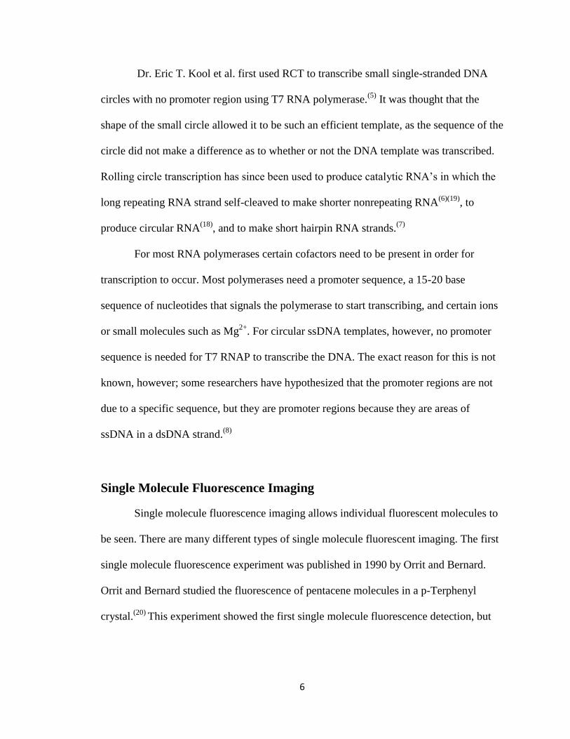
Figure 3: Picture of a microscope set up

to use TIRF. The prism directs the light

from the laser to hit the surface at an

angle that can create the evanescent wave

needed for TIRF.(24)

9

used to reduce the amount of fluorescence background from out-of-focus regions. Using

TIRF only molecules within 100-200nm of the surface fluoresce.(26)

TIRF is great for

solution experiments in which there might be other fluorescent molecules out of focus

that can overwhelm the fluorescence of a single molecule in solution. Because the

molecules are in solution, the molecules of interest may have to be tethered to the surface

to keep them from floating away. TIRF has been done on experiments with living cells as

well as in vitro experiments.

In TIRF the excitation light travels through the glass coverslip at a high incident

angle creating an evanescent wave at the glass/ water or buffer interface. This evanescent

wave excites the fluorophores close to the surface (less than 200nm). The strength of the

evanescent wave decays as it travels farther from the surface.(27)

The easiest way to add

TIRF to a microscope is to add a prism. The prism directs the excitation light toward the

interface of the glass/ liquid at an angle that is slightly larger than the critical angle for

total internal reflection.(28)

Figure 3 shows a typical microscope set up for TIRF. Part of

the excitation light from the laser is directed into the prism. The prism directs the light at

the correct angle to create an evanescent wave. The light from the excited fluorescent

molecules are directed to the detector (in this case the CCD camera and PMT cabinet) in

the same way as non-TIRF microscopy.

Overview of this project

We are determining the rate of T7 RNA polymerase by recording the changes in

intensity of a fluorescent molecule during transcription. We used the fluorescent

molecule Cy3 shown in Figure 4. Cy3 is a fluorescent molecule that is used in many

10

single molecule studies because of its brightness and stability. Cy3 is also sensitive to its

environment, which makes it a good reporter molecule. Luo et al. showed that Cy3’s

intensity will increase when T7 DNA polymerase binds to it during replication.(29)

They

hypothesized that this was due to the polymerase limiting the range of motion of the

fluorophore and therefore not allowing the Cy3 molecule to get rid of the energy through

vibrations, only by releasing a photon. The constraints on Cy3 should work similarly in

the case of T7 RNA polymerase because the RNAP will put the same constraints on the

Cy3 molecule that the DNAP would.

A circular DNA template was chosen because the polymerase will transcribe the

circle multiple times, thus giving more data

because there will be multiple interactions with

the Cy3 before termination. The multiple

interactions also omit the need to label the DNA in

multiple places. To image the Cy3 labeled DNA

as it is being transcribed, the T7 RNAP, NTPs,

DTT, Trolox, and Cy3 labeled circular DNA is

loaded into a flow cell in 0.5x transcription buffer.

Transcription buffer is a mixture of salts and ions that produce a good ion and pH

environment for the enzyme. The flow cell is imaged under a fluorescent microscope and

the images are recorded sequentially, making movies. Each movie is composed of 1250

frames with 48 milliseconds between frames. The movie is then processed using a Matlab

script, and the individual fluorescent spots are selected and their intensity over time is

Figure 4: Cy3 molecule/ pseudobase that

is inserted into the DNA strand. The

image is from idtdna.com.

11

graphed. The intensity graphs show quasi-periodic modulations that are due to the

intensity changes of the Cy3 as the T7 RNAP transcribes the circle.

The RNAP resting directly on a glass surface has been shown to decrease the

efficiency of the enzyme,(30)

probably due to steric effects. If the polymerase is adsorbed

on the surface of the glass, there will be fewer degrees of freedom for the polymerase to

move while transcribing. The polymerase will adsorb onto a glass surface, unless the

glass is protected by a coating of another protein. Although the intensity modulations did

occur when the polymerase is directly on glass, the surface of the flow cell was coated to

determine whether the processivity of the enzyme would increase. Two coatings, bovine

serum albumin (BSA) and poly-L-lysine, were used to determine which, if either, worked

better than uncoated glass. A thin layer of the protein was formed between the glass of

the enzyme, and then the reaction was run in the coated flow cell and recorded.

Determination of Transcription Rate

Many experiments have been performed to determine the transcription rate of

RNA polymerases. If we can measure the rate of transcription for a particular polymerase

then we can figure out what environmental factors we can use to slow down or speed up

the polymerase. Ensemble techniques used to be the only ones available to determine the

rate. The problem with ensemble techniques is one only obtains an average rate for all of

the polymerases in the sample. With single-molecule techniques one can look at each

individual polymerase’s rate and pausing. Generalizations for a particular polymerase can

still be made; however, more information will be known about the differences of

individual polymerases.

12

When single molecule techniques were used to determine the transcription rate, a

variety of pausing times were found, especially for E.coli RNA polymerase, a very well

studied multi-subunit RNAP. Pausing times from 1 second to 30 minutes were found for

this enzyme.(31)

T7 RNAP does not pause as often or for as long as E.coli RNAP, so,

when determining the transcription rate, pausing is not a large concern. Certain DNA

sequences such as 5’- ATCTGTT-3’ are known to cause pausing. However, these

sequences are not in the circular template that we will be using.(5)

A variety of experiments has been done to determine the rate of T7 RNAP. Some

of the techniques will be described below, but a discussion on some of the published rates

will be discussed here. Table 1 shows four published rates and the technique and some

parameters used to calculate the rate. As shown in the table, there is a wide range of rates

depending on the NTP concentration and the technique used. The highest rate, 129nt/sec,

was calculated from a single molecule force measurement of T7 RNAP transcribing λ

Technique Concentration

of NTPs

DNA

template

Published

Rate

Reference

Number

Estimated

using

computer

simulation

Excess pT3/T7luc

(linear) 97nt/sec 32

Single

molecule

force

measurements

30-590μM λ DNA 129 nt/sec 33

Single

molecule

FRET

Very low

Multiple T7

promoters

(linear)

20-60 nt/sec 34

Single

molecule

fluorescent

tracking of T7

RNAP

0.2mM λ DNA 42 nt/sec 35

Table 1: Table of different transcription rates and the techniques used to calculate them for T7 RNAP.

13

DNA. There are two single molecule fluorescence techniques shown in Table 1. One

used single molecule FRET and published a rate of 20-60 nt/sec, and the second used a

fluorescently labeled T7 RNAP and published a rate of 42 nt/sec.

Ensemble Techniques

The rate of a polymerase has historically been determined by quantifying the

amount of RNA that was produced. One method for making this determination was

described in a paper by Guerniou et al. in 2005. RNA was transcribed in vitro then

purified. The purified RNA was annealed with a radioactive phosphate labeled DNA

primer. The labeled DNA was extended by reverse transcription, and then the DNA was

run in a polyacrylamide gel. The DNA was imaged using phosphorimager screens and

quantified.(31)

The amount of transcript obtained after a certain amount of time by a

certain quantity of enzyme was used to determine the transcription rate.

A radioactive label was used because DNA can be more precisely quantified

using radioactive labels than by using fluorescent dyes such as ethidium bromide and

SYBER green. One drawback to this technique is that it is an indirect approach. DNA

made from the RNA that was transcribed is measured. Another drawback of this

technique is that the process is assumed to be homogeneous. Every enzyme of the same

type is assumed to behave the same way, and every DNA template is assumed to be the

same. Although enough enzymes are used that one or two slow ones will not affect, the

overall group rate, the individual nuances from each enzyme is missed. Pausing is

another concern. The pausing can be counted in the transcription time giving an overall

lower transcription rate. Overall a lot of information is lost or overlooked in ensemble

techniques.

14

Single Molecule Techniques

Single molecule techniques show the individual nuances of the

polymerases, and can indicate the difference between pausing and elongation. A high

variability of transcription rates, standard deviation of about 30%, have been found for

T7 RNAP using single molecule techniques.(13)

This variability is due to the variation of

the single polymerases that are usually averaged in ensemble experiments. One of the

most popular single molecule techniques, especially in the early part of the decade, was

to connect the DNA to beads and measure the changes in the beads. Bustamante et. al.

used a flow controlled optical trap with fluorescence microscopy to determine the rate of

E. coli RNAP. The template DNA was tethered between two beads. As the RNAP

transcribes the DNA, it will bring the two beads closer together. The distance between the

two beads was measured with fluorescence microscopy.(36)

Another way to gain information on the transcription of single RNA polymerase

molecules is to measure the force of the RNA polymerase during transcription. When a

RNA polymerase transcribes DNA to RNA, the energy from breaking the triphosphate

bond in the nucleotide triphosphate that it added to the RNA chain propels the RNAP

down the DNA strand. Gelles et. al. attached the DNA template to a polystyrene bead that

was held in place using an optical trap. As the RNAP transcribed the DNA template, it

pulled the DNA template, which, in turn, pulled the polystyrene bead. The polystyrene

bead could only move a little because it was in the optical trap, so the force that was

applied to the optical trap to keep the bead in there was related to the transcription of the

RNAP.(33)

15

Some have used single molecule fluorescence techniques to observe RNAP

transcription. Forgoing an optical trap means that one does not need to add a bead to the

reaction, and that one will be measuring or visualizing the actual components of

transcription (DNA, RNA, or RNAP) instead of a bead that is attached to one of the

components (usually DNA). Berge et al. combed the template DNA onto a glass surface

and added fluorescently labeled uracil triphosphates along with the other nucleotide

triphosphates in order to fluorescently label the RNA. They allowed transcription to

occur and then caused it to pause by removing the nucleotide triphosphates. Any

fluorescence that was not attached to RNA would be removed and then the glass was

imaged. Fluorescent lines from the RNA were made, and they could determine how many

bases were added into the growing RNA polymer by measuring the length of the

fluorescent line. Multiple RNAs could be seen in the same field of view allowing more

data to be collected at once. (37)

Experimental

Microscope Setup

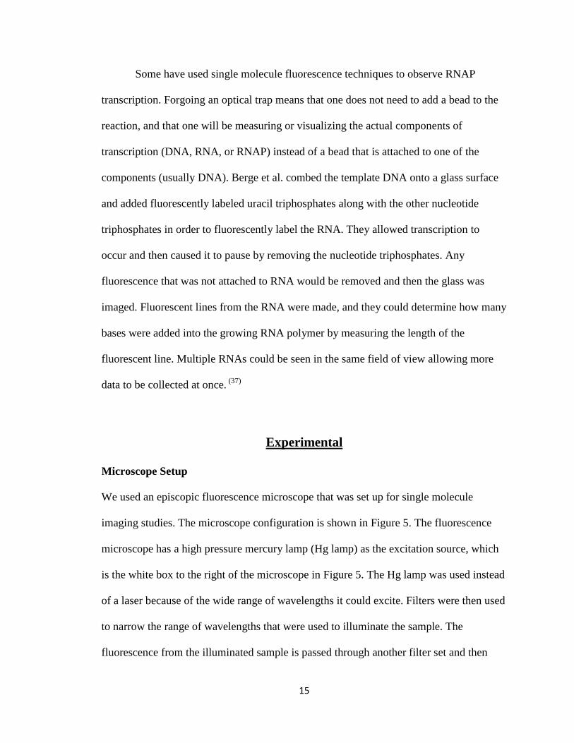
We used an episcopic fluorescence microscope that was set up for single molecule

imaging studies. The microscope configuration is shown in Figure 5. The fluorescence

microscope has a high pressure mercury lamp (Hg lamp) as the excitation source, which

is the white box to the right of the microscope in Figure 5. The Hg lamp was used instead

of a laser because of the wide range of wavelengths it could excite. Filters were then used

to narrow the range of wavelengths that were used to illuminate the sample. The

fluorescence from the illuminated sample is passed through another filter set and then

16

directed through the optical splitter

(black box to the left of the

microscope pictured in Figure 5). The

emitted light is then directed to the

CCD camera (red and silver camera

to the left of the optical splitter in

pictured in Figure 5), which detects

the fluorescence and sends the image

to the computer.

TIRF was not used in this microscope because our background was low enough to

image single molecules in solution without it. TIRF is often used in fluorescent studies of

cells in which one does not have as

much control over the solutions. For

our experiments, all of our solutions

except our labeled DNA were shown

not to be fluorescent.

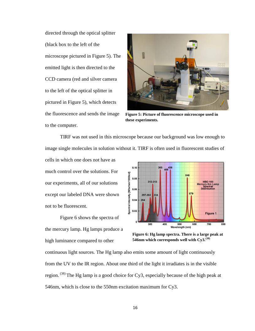
Figure 6 shows the spectra of

the mercury lamp. Hg lamps produce a

high luminance compared to other

continuous light sources. The Hg lamp also emits some amount of light continuously

from the UV to the IR region. About one third of the light it irradiates is in the visible

region. (38)

The Hg lamp is a good choice for Cy3, especially because of the high peak at

546nm, which is close to the 550nm excitation maximum for Cy3.

Figure 5: Picture of fluorescence microscope used in

these experiments.

Figure 6: Hg lamp spectra. There is a large peak at

546nm which corresponds well with Cy3.(38)

17

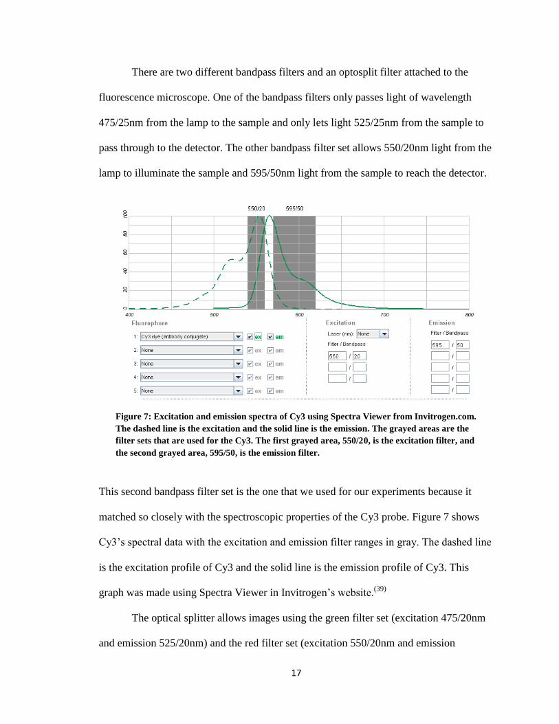
There are two different bandpass filters and an optosplit filter attached to the

fluorescence microscope. One of the bandpass filters only passes light of wavelength

475/25nm from the lamp to the sample and only lets light 525/25nm from the sample to

pass through to the detector. The other bandpass filter set allows 550/20nm light from the

lamp to illuminate the sample and 595/50nm light from the sample to reach the detector.

This second bandpass filter set is the one that we used for our experiments because it

matched so closely with the spectroscopic properties of the Cy3 probe. Figure 7 shows

Cy3’s spectral data with the excitation and emission filter ranges in gray. The dashed line

is the excitation profile of Cy3 and the solid line is the emission profile of Cy3. This

graph was made using Spectra Viewer in Invitrogen’s website.(39)

The optical splitter allows images using the green filter set (excitation 475/20nm

and emission 525/20nm) and the red filter set (excitation 550/20nm and emission

Figure 7: Excitation and emission spectra of Cy3 using Spectra Viewer from Invitrogen.com.

The dashed line is the excitation and the solid line is the emission. The grayed areas are the

filter sets that are used for the Cy3. The first grayed area, 550/20, is the excitation filter, and

the second grayed area, 595/50, is the emission filter.

18

595/50nm) to be seen in the same field of view in two separate channels. On the right

side of the image is the red channel and on the left side is the green channel. The optical

splitter was helpful in experiments because it showed that the spots appeared only in the

red channel and therefore would not likely be adventitious (impurity) fluorescence.

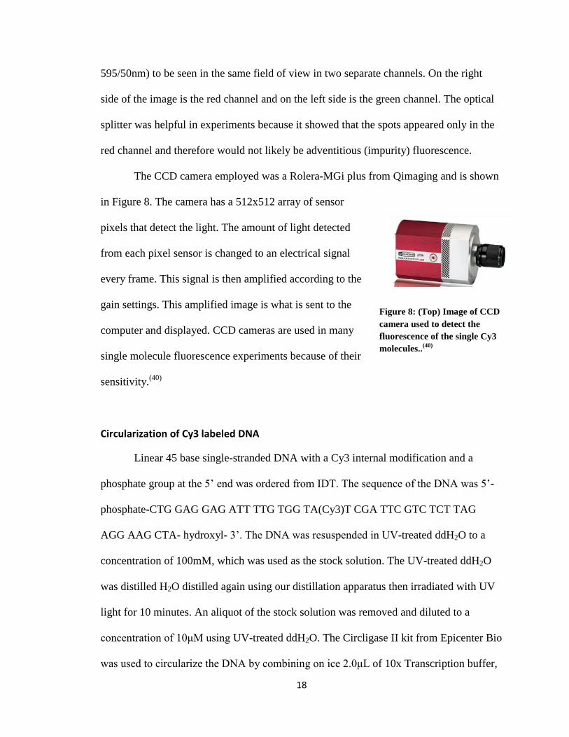
The CCD camera employed was a Rolera-MGi plus from Qimaging and is shown

in Figure 8. The camera has a 512x512 array of sensor

pixels that detect the light. The amount of light detected

from each pixel sensor is changed to an electrical signal

every frame. This signal is then amplified according to the

gain settings. This amplified image is what is sent to the

computer and displayed. CCD cameras are used in many

single molecule fluorescence experiments because of their

sensitivity.(40)

Circularization of Cy3 labeled DNA

Linear 45 base single-stranded DNA with a Cy3 internal modification and a

phosphate group at the 5’ end was ordered from IDT. The sequence of the DNA was 5’-

phosphate-CTG GAG GAG ATT TTG TGG TA(Cy3)T CGA TTC GTC TCT TAG

AGG AAG CTA- hydroxyl- 3’. The DNA was resuspended in UV-treated ddH2O to a

concentration of 100mM, which was used as the stock solution. The UV-treated ddH2O

was distilled H2O distilled again using our distillation apparatus then irradiated with UV

light for 10 minutes. An aliquot of the stock solution was removed and diluted to a

concentration of 10μM using UV-treated ddH2O. The Circligase II kit from Epicenter Bio

was used to circularize the DNA by combining on ice 2.0μL of 10x Transcription buffer,

Figure 8: (Top) Image of CCD

camera used to detect the

fluorescence of the single Cy3

molecules..(40)

19

1.0μL of MnCl2, 120pmol of linear DNA, and 2.0μL of CircligaseII ssDNA ligase. The

solution was incubated at 60°C for 2 hours and 80°C for 10 minutes. After the solution

cooled to room temperature, it was ethanol precipitated and resuspended in UV-treated

ddH2O.

In Vitro Rolling Circle Transcription:

RNA was made by combining on ice 2pmol of circular DNA with Cy3 internal

label, 2µL 10x transcription buffer (Ambion), 2µL 100mM DTT, 3.5µL 10mM NTP mix

(Invitrogen), 20U Scriptguard RNase inhibitor (Epibio), and 40U T7 RNAP (Ambion) in

a final volume of 20µL. The solution was incubated at 37°C for 3 hours. The product was

treated with Baseline Zero DNase(Epicenter Bio) to remove the DNA. The remaining

RNA was ethanol precipitated and resuspended in UV treated ddH2O. The RNA was

analyzed through an agarose gel and fluorescence microscopy.

The RNA was run in a 1.2% Agarose RNA flashgel (Lonza) along with RNA

Century Marker (Ambion) and the transcription solution before incubation at 37°C as a

control. The gel was run at 225V for 5 minutes or until the components of the ladder were

sufficiently separated. The flashgel was imaged using filter set 2 (for ethidium bromide

stained gels) of the Alpha Innotech gel imager. The gel was then allowed to set in the

dark for 15 minutes and then imaged again using filter set 2 of the gel imaging system.

The dye that is in the flashgel does not bind to RNA as well as DNA, and many times the

RNA bands will be invisible while the gel is running. Letting the flashgel sit for 15-30

minutes before being imaged helped to intensify the bands so they can be imaged.(41)

The purified RNA was annealed with a 45nt DNA complement labeled with

rhodamine at the 5' end (IDT) by combining the RNA and the DNA in a microcentrifuge

20

tube in a 1:5 ratio of RNA to DNA then heating the solution to 70°C for 5 minutes in a

digital dry bath then allowing it to slowly cool to room temperature. The annealed

DNA:RNA was filtered with a Microcon YM-30 centrifuge filters (Millipore) to remove

the excess 45nt rhodamine labeled DNA. The RNA:DNA hybrid was combed onto a

clean glass coverslip and imaged under N2 using a Hg lamp as the excitation source with

excitation filters at 550/20nm and emission filters at 595/50nm. The movies were taken

using QCapture Pro software. An EM gain of 2500 was used to take the images and the

time between each frame was 140msec.

Cleaning Glass and Making a Flowcell

Glass coverslips (Fisher Scientific cat # 12-548-B) were lightly scratched using a

diamond scribe to produce fiducial marks and then sonicated in acetone for 20 minutes.

The glass coverslips were next rinsed with UV treated ddH2O, dried with N2 and then

irradiated with UV light for 15 minutes. The coverslip was imaged scratch side up. The

scratch was used to quickly focus on the surface of the coverslip. To make the flow cell,

two holes were drilled in a glass slide (Fisher Scientific catalog #12-544-6) using a

Dremel tool with a diamond bit. The glass slide was sonicated in acetone for 20 minutes

then rinsed in UV treated ddH2O, dried with N2 then irradiated with UV light for 15

minutes. A schematic of the construction of the flow cell is shown in Figure 9 (left).

Double-sided tape was placed on the long edges of the clean glass slide. A clean glass

coverslip was placed on top of the tape over the drilled holes scratch side down and the

excess tape was removed. Epoxy was used to seal the places between the glass slide and

glass coverslip where there is no tape. The epoxy was allowed to completely dry before

any solution was added.

21

Later in the project a

second, simpler design for the

flow cell was made that omitted

the epoxy. A clean glass

coverslip was placed on top of

the tape over the drilled holes

scratch side down and the

excess tape was removed. A

schematic for the construction

of this flow cell is shown in

Figure 9 (right). The liquid still

stayed inside of the flow cell

because the total volume was

such a small amount (40μL),

and the omission of the epoxy

allowed liquid to be flowed in

and out by wicking with a Kim

wipe.

Photostability of Cy3 labeled DNA:

To image the Cy3 labeled DNA on glass, 10μL of 100nM Cy3 labeled DNA was

deposited onto a clean glass coverslip and allowed to incubate for 10 minutes. The

coverslip was rinsed once with UV treated ddH2O and dried with N2. To image the Cy3

Figure 9: Cartoon of the making of the two types of flow cell.

To the left is the first where the glass coverslip is attached to

the slide with double-sided tape and the other two ends are

sealed with epoxy. To the right is the flow cell where the glass

coverslip is attached to the slide with the double-sided tape

and the other two ends are left open to allow liquid to be

wicked through.

22

labeled DNA in H2O and in 1x transcription buffer (40 mM Tris pH 7.8, 20 mM NaCl, 6

mM MgCl2, 2 mM Spermidine HCl, 10 mM DTT), 50 fmol of Cy3 labeled DNA and

8.0µL of H2O or transcription buffer was pipetted into the flowcell. The Cy3 labeled

DNA in either H2O or 1x transcription buffer and Trolox solution was made by

combining and adding to the flow cell 2μL of 150nM Cy3 labeled DNA, 6.0 µL H2O or

transcription buffer, and 2.0 µL 0.5mM Trolox. All images were taken under N2 using a

Hg lamp as the excitation source with excitation filters at 550/20nm and emission filters

at 595/50nm. The movies were recorded using QCapture Pro software. An EM gain of

2500 was used to take the images, and the time between each frame was 141msec for the

Cy3 labeled DNA on glass, in water and in a water Trolox solution; the time between

each frame for the Cy3 labeled DNA in 1x transcription buffer and in 1x transcription

buffer with Trolox is 141msec. The movies were converted to AVI files using Image J.

The AVI files were then run through a Matlab script where each individual spot’s

intensity was graphed over time. Using the graph and the chart of the intensities, the

frame in which each spot photobleached was determined. A graph was made of the

photobleaching times using Microsoft Excel, and the photochemical half-life of the Cy3

labeled DNA was determined from the graphs.

Fluorescent Imaging of Transcription process

2μL of 1U/μL T7 RNAP(Ambion) was pipetted into a clean flow cell and allowed

to incubate for 10 minutes. The flow cell was then rinsed with UV-treated ddH2O twice

and 0.5x transcription buffer twice. DTT and NTP mix was added to the flowcell. 2μL of

150nM Cy3 labeled circular DNA was added to the flow cell and immediately imaged.

The movies were taken on an episcopic fluorescent microscope with a Hg lamp as the

23

excitation source and a CCD camera as the detector. An excitation filter at 550/20nm and

an emission filter at 595/50nm allowed only certain wavelengths through to the sample

and the detector respectively. Movies were taken, using QCapture Pro software with an

EM gain of 2500 and an exposure time of 25milliseconds. The image was 512x256

pixels. The time between each frame of the movie was 48 milliseconds. The exposure

time and the size of the image could be changed to obtain a lower time between frames.

The lowest possible time between frames that the CCD camera with the QCapture Pro

software can obtain is ~33 milliseconds between frames.(33)

The lowest exposure time

that could be used and still obtain images of single molecules was 25milliseconds. The

size of the image was reduced by half to obtain a better time between frames while still

showing both channels from the optical splitter.

BSA Coating Flow cells

A clean flow cell was constructed as described above. 25mg of BSA(Promega)

was dissolved in 10mL PEM-80 buffer. The BSA solution was filtered using YM-100

centrifuge filter from Millipore. 40μL BSA solution was flowed into the flow cell and

was incubated at room temperature for 10 minutes. The flow cell was rinsed with 100μl

of PEM-80 buffer to remove excess BSA.(42)

Poly-L-lysine coated flow cells

A glass coverslip was cleaned as described above. The coverlip was placed in a

new clean plastic Petri dish. Then 1mL of 0.1% w/v Poly-L-lysine solution in water

(Sigma Aldrich) was pipetted onto the glass coverslip and incubated at room temperature

for 5 minutes. The poly-L-lysine solution was pipetted off of the coverslip and the

coverslip dried overnight in the petri dish. The coverslip was then rinsed with UV-treated

24

ddH2O and dried with N2. The flow cell was then made by using double sided tape to

attach the poly-L-lysine coated coverslip, coated side down to the clean glass slide along

the long edge of the glass slide.

Results

Circularizing 45nt single-stranded DNA with internal Cy3 modification

We ordered a 45 base single-stranded oligonucleotide with an internal Cy3

modification from IDT. The sequence of the DNA oligo was 5’- phosphate-CTG GAG

GAG ATT TTG TGG TA(Cy3)T CGA TTC GTC TCT TAG AGG AAG CTA-

hydroxyl-3’. The DNA was suspended in UV treated ddH2O to a final concentration of

100μM that was used as the stock solution. An aliquot of the stock solution was diluted to

a concentration of 10 μM with UV treated ddH2O. This solution was used as the working

solution (the solution that was circularized). The UV-Vis spectrum of the working

solution was taken using the NanoDrop 2000. The UV treated ddH2O was used as the

blank. The UV-Vis spectrum of the linear DNA with the Cy3 internal modification is

shown in Figure 10 (top). There was a good absorbance peak at 260nm (where DNA

absorbs) and another smaller peak at 550 where Cy3 absorbs. Using Beer’s law, the

concentration of the DNA was found to be 0.013M or 13mM.

0.455= (33cm-1

•M-1

)(1cm)(c) [Equation 1]

25

The DNA oligo was circularized using the Circligase II ssDNA kit from Epicenter

Bio. The circularization solution was incubated at 60°C for 2 hours and 80°C for 10

minutes. The first incubation temperature is the optimum temperature for the enzyme to

work and is the time that

it should circularize the

ssDNA, and the second

temperature should

deactivate the enzyme.

An aliquot of the

circularized solution was

removed and stored at -

20°C and the rest was

treated with Exonuclease

I to digest any remaining

linear DNA so all that

should remain in our

solution was circular

DNA. The DNA was

ethanol precipitated and then resuspended in 1x TE buffer. The ethanol precipitation

concentrated the DNA and removed excess salts. Now, only the DNA and the 1x TE

buffer was in the solution.

A UV-Vis spectrum of the resuspended circular ssDNA was taken using the

Nanodrop. 1x TE buffer was used as the blank and the spectra is shown in Figure 10

Figure 10: (Top) UV-Vis spectra of linear ssDNA with Cy3 inserted

into the phosphate backbone. (Bottom) UV-Vis spectra of circular

ssDNA with Cy3 inserted into the phosphate backbone.

26

(bottom). There was a good absorbance peak at 260nm, where DNA absorbs, of 0.363.

The Cy3 absorbed at 555nm instead of 550nm. This red shift of the dye could be due to

the added constraints from the circularization of the DNA. This shift shows how sensitive

the Cy3 dye is to changes in its environment.

Using Beer’s law, the concentration of the DNA was found to be 0.011M or

11mM when the extinction coefficient was 33cm-1

•M-1

.

0.363= (33cm-1

•M-1

)(1cm)(c) [Equation 2]

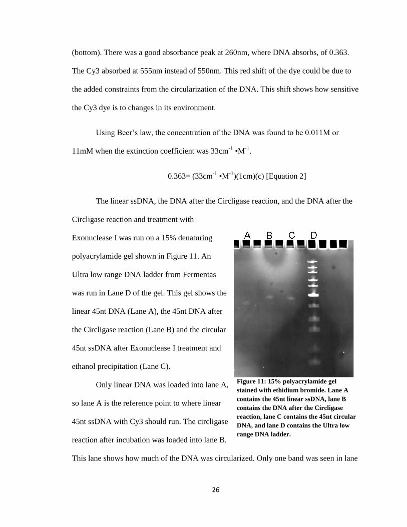
The linear ssDNA, the DNA after the Circligase reaction, and the DNA after the

Circligase reaction and treatment with

Exonuclease I was run on a 15% denaturing

polyacrylamide gel shown in Figure 11. An

Ultra low range DNA ladder from Fermentas

was run in Lane D of the gel. This gel shows the

linear 45nt DNA (Lane A), the 45nt DNA after

the Circligase reaction (Lane B) and the circular

45nt ssDNA after Exonuclease I treatment and

ethanol precipitation (Lane C).

Only linear DNA was loaded into lane A,

so lane A is the reference point to where linear

45nt ssDNA with Cy3 should run. The circligase

reaction after incubation was loaded into lane B.

This lane shows how much of the DNA was circularized. Only one band was seen in lane

Figure 11: 15% polyacrylamide gel

stained with ethidium bromide. Lane A

contains the 45nt linear ssDNA, lane B

contains the DNA after the Circligase

reaction, lane C contains the 45nt circular

DNA, and lane D contains the Ultra low

range DNA ladder.

27

B and it ran slower than the band in lane A. This shows that the majority of the linear

DNA was circularized in the reaction. The band in lane C ran slower than the band in

lane A and the same as the band in lane B. Because lane C contained the DNA after

treatment with Exonuclease, this is further proof that the bands in lanes B and C are

circular because Exonuclease only digests linear DNA.

The gel in Figure 11 shows that the internal Cy3 modification in the DNA did not

affect the circularization of the DNA. Almost all of the linear DNA that was added to the

circularization reaction was circularized. The addition of the Cy3 probably did not affect

the circularization because it is inserted internally, not on the ends. The Cy3 was added in

the middle of the linear DNA at least 20 bases away from either one of the edges. The

purified circular DNA was used as the DNA template in RNA transcription.

InVitro Transcription of Cy3 modified circular ssDNA with T7 RNAP

To ensure that the T7 RNAP would transcribe the modified circular DNA, we first

ran the transcription experiment in vitro and visualized it with agarose gel

electrophoresis. An aliquot of the components of the transcription reaction were stored at

-20ºC before incubation. This aliquot was used as the control, as the RNAP should not

transcribe at -20ºC, so all of the reaction components are in there, but no RNA, so only a

DNA band should be seen in the gel. The circular DNA was transcribed with T7 RNAP

at 37ºC, and an aliquot of this mixture was stored at -20ºC. This aliquot should have both

the template DNA and the RNA. The rest of the transcription mixture was treated with

DNase to remove the DNA template, and then the remaining RNA was ethanol

precipitated and resuspended in 1x TE buffer. The concentration of the RNA was

28

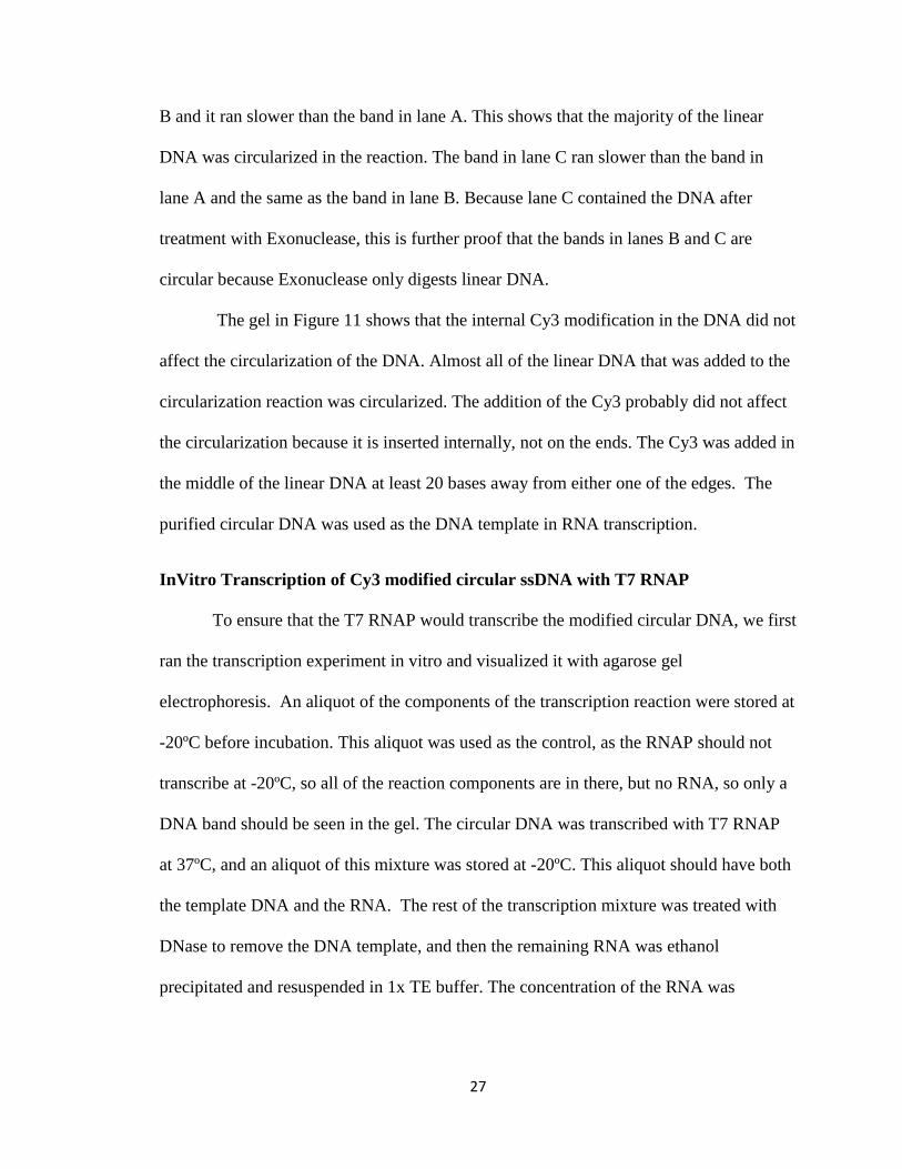
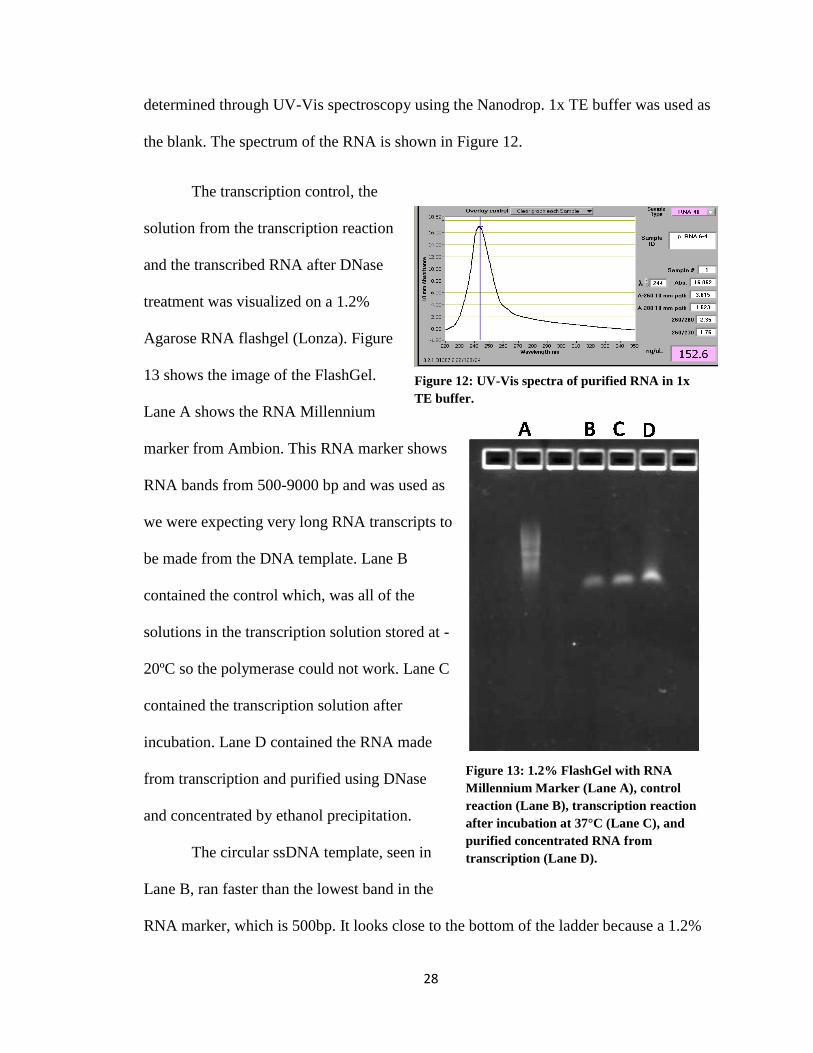
determined through UV-Vis spectroscopy using the Nanodrop. 1x TE buffer was used as

the blank. The spectrum of the RNA is shown in Figure 12.

The transcription control, the

solution from the transcription reaction

and the transcribed RNA after DNase

treatment was visualized on a 1.2%

Agarose RNA flashgel (Lonza). Figure

13 shows the image of the FlashGel.

Lane A shows the RNA Millennium

marker from Ambion. This RNA marker shows

RNA bands from 500-9000 bp and was used as

we were expecting very long RNA transcripts to

be made from the DNA template. Lane B

contained the control which, was all of the

solutions in the transcription solution stored at -

20ºC so the polymerase could not work. Lane C

contained the transcription solution after

incubation. Lane D contained the RNA made

from transcription and purified using DNase

and concentrated by ethanol precipitation.

The circular ssDNA template, seen in

Lane B, ran faster than the lowest band in the

RNA marker, which is 500bp. It looks close to the bottom of the ladder because a 1.2%

Figure 12: UV-Vis spectra of purified RNA in 1x

TE buffer.

A BA B

Figure 13: 1.2% FlashGel with RNA

Millennium Marker (Lane A), control

reaction (Lane B), transcription reaction

after incubation at 37°C (Lane C), and

purified concentrated RNA from

transcription (Lane D).

29

Agarose gel cannot separate small DNA or RNA molecules well. Lane C shows the RNA

that was made during transcription and the template DNA. The band ran the same as the

one in Lane B but was brighter, indicating that there were more nucleic acids in the band.

Lane D shows the purified and concentrated RNA. A band is at the same position as the

other two lanes, but there is a smear above the band. This smear is due to the different

lengths of RNA that were produced during rolling circle transcription (RCT). The

different lengths of RNA are too close together to be separated into distinct bands by this

gel. This smear is seen in Lane D but not in Lane C because the RNA in Lane D is more

concentrated than the RNA in Lane C. The same RNA is in the lane but there is not

enough RNA to be visualized.

According to the gel, most of the RNA produced is 1000 bases or less, but some

of the RNA is up to 6000 bases in length. In terms of how many revolutions around the

DNA circle the polymerase traveled, the majority of the time the RNAP transcribed the

circle 21 times or less and, in some cases,

transcribed the circle up to 130 times. The Cy3

in the phosphate backbone of the DNA did not

stop transcription. For the single molecule

fluorescence studies, 21 revolutions would be

plenty of time to watch the changes in

intensity and find a pattern.

To further prove that RNA much

longer than the template DNA was produced

the RNA was purified with gel extraction and

Figure 14: Fluorescence image of RNA

annealed with short rhodamine labeled

DNA and combed onto a clean glass

surface. The red arrow shows a long RNA

strand.

30

ethanol precipitation and then annealed with a 45nt DNA complement labeled with

rhodamine at the 5' end. The DNA:RNA hybrid was combed onto a clean glass surface

and imaged using the fluorescence microscope.

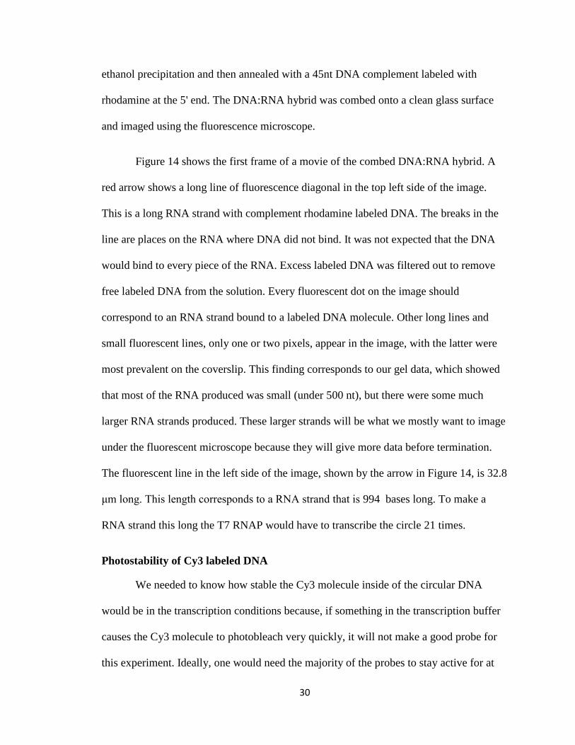
Figure 14 shows the first frame of a movie of the combed DNA:RNA hybrid. A

red arrow shows a long line of fluorescence diagonal in the top left side of the image.

This is a long RNA strand with complement rhodamine labeled DNA. The breaks in the

line are places on the RNA where DNA did not bind. It was not expected that the DNA

would bind to every piece of the RNA. Excess labeled DNA was filtered out to remove

free labeled DNA from the solution. Every fluorescent dot on the image should

correspond to an RNA strand bound to a labeled DNA molecule. Other long lines and

small fluorescent lines, only one or two pixels, appear in the image, with the latter were

most prevalent on the coverslip. This finding corresponds to our gel data, which showed

that most of the RNA produced was small (under 500 nt), but there were some much

larger RNA strands produced. These larger strands will be what we mostly want to image

under the fluorescent microscope because they will give more data before termination.

The fluorescent line in the left side of the image, shown by the arrow in Figure 14, is 32.8

μm long. This length corresponds to a RNA strand that is 994 bases long. To make a

RNA strand this long the T7 RNAP would have to transcribe the circle 21 times.

Photostability of Cy3 labeled DNA

We needed to know how stable the Cy3 molecule inside of the circular DNA

would be in the transcription conditions because, if something in the transcription buffer

causes the Cy3 molecule to photobleach very quickly, it will not make a good probe for

this experiment. Ideally, one would need the majority of the probes to stay active for at

31

least 30 seconds. This is about half of the length of other recordings reported in this

thesis. To measure the photochemical half-life, we determined the photostabilty of the

Cy3 in three different environments: dry on glass, in water, and in 1x transcription buffer.

Transcription experiments cannot be

performed dry on glass or in water. The salts

that are in the transcription buffer are required

for the polymerase to transcribe efficiently.

Therefore, while determining the

photochemical half-life times for the Cy3

labeled DNA water and dried on glass is useful

for comparison, the environment that needs to

have a long photochemical half-life is the Cy3

labeled DNA in transcription buffer. If the

photochemical half-life was found to be too short then parameters, including salt

concentration, could be modified to lengthen the photochemical half-life.

To determine the photostabilty of Cy3, movies were taken of the Cy3 labeled

DNA in different environments: on glass, in H2O, and in transcription buffer. Figure 15

shows the first frame of a movie of Cy3 labeled DNA in transcription buffer. The dots of

intensity are single fluorescent molecules. Using SpotSelect, a script run in Matlab,

places of intensity are labeled as spots, and the intensity over time for each of the spots is

graphed. The intensity over time data for each spot is filtered using a Weiner2 filter. The

Weiner2 filter reduces the noise that is seen, so the photobleaching step can more clearly

be seen. The time that each fluorescent molecule photobleached is recorded and graphed.

Figure 15: Fluorescence image of Cy3

labeled DNA in transcription buffer. This

image is the 1st frame of a 500 frame movie.

32

In this way the photochemical half-

life of the Cy3 in each environment

can be determined.

When photobleaching occurs

the fluorescent intensity of the Cy3

molecule should decrease to

background levels in one frame.

Figure 16 shows two graphs of two

different spots in the movie. Both

show one-step photobleaching. In

one-step photobleaching, the

intensity drops to zero or

background in one step. One-step

photobleaching is a characteristic of single molecule fluorescence techniques and a way

to prove that what one is looking at is a single molecule. Some of the molecules

fluoresced throughout the entire movie but most photobleached sometime during the

movie. Each movie was 750 frames long and 140 milliseconds between frames, so each

movie was a total of 105 seconds long.

Each graph of each individual spot in a movie was run through a set of criteria to

be certain it was a single molecule. The first criteria is that the spot was above the

minimum threshold value determined by the SpotSelect script. A description of the

threshold can be found in Appendix D. The second criterion is that the spots did not show

two-step or multistep photobleaching. If they showed single-step photobleaching, it

Figure 16: Two graphs showing the intensity

over time (seconds) of a Cy3 labeled DNA in

transcription buffer. Both graphs show one-step

photobleaching which proves that there was

only one molecule producing the light.

33

proved that they were single molecules. The last criterion was that the spots’ intensities

were not larger than 2000. Most of the single molecule spots had intensities between 500

and 1200. If the spot passed the test to be a single molecule, the time that it

photobleached was recorded. If the molecule did not photobleach during the movie, the

end time of the movie was recorded. This process was done for spots in movies for each

environment tested.

For each environment, the number of molecules active at increments of 5 seconds

was graphed and fit to a decaying exponential curve. The total number of molecules that

were analyzed for a particular environment is shown in the number of molecules at time

zero. Figure 17 shows the exponential graphs for Cy3 labeled DNA in three different

environments: dry on glass under N2, in UV-treated ddH2O under N2, and in 1x

Figure 17: Graphs showing the number of fluorescent molecules active after a given time in a movie.

These data points were fit to an exponential curve. The top graph shows the number of molecules

active at varying times for the Cy3 labeled DNA dried on a glass coverslip, the bottom left graph

shows the number of molecules active at varying times for the Cy labeled DNA in water, and the

bottom right graph shows the number of molecules active at varying times for the Cy3 labeled DNA

in 1x transcription buffer.

34

transcription buffer under N2.

For each of the environments, we looked at over 100 spots to get a good sampling

of the times they photobleached. The Cy3 labeled DNA in transcription buffer showed

the best exponential decay, and, by the end of the sampling time, the majority of the

molecules had photobleached. The exponential fit was not quite as good in the graph of

the Cy3 labeled DNA in water as in transcription buffer, but it was good enough to give

us a value. For the Cy3 labeled DNA that was dried on glass, the decay was almost linear,

not exponential. For all of the environments the majority of the molecules had

photobleached by the end of the experimental time.

From the graphs, the photochemical half-life of the Cy3 labeled DNA in each of

the environments was calculated. Table 2 shows the calculated half-life. The

photochemical half-life of the Cy3 labeled DNA on glass under N2 was 37 seconds, in

water under N2 was 25 seconds, and in 1x transcription buffer under N2 was 17 seconds.

The photochemical half-life of the Cy3 was longest dried on glass and shortest in 1x

transcription buffer, which was unexpected. One reason for this result could be that there

was very little oxygen (less than 1%) around the Cy3 molecules that were dried on glass,

but for the two samples in liquid, there could still have been a high percentage of O2

causing the fluorophores to photobleach faster.

35

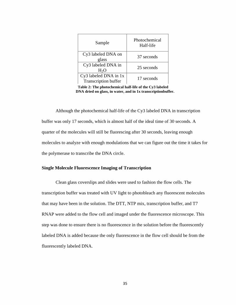
Table 2: The photochemical half-life of the Cy3 labeled

DNA dried on glass, in water, and in 1x transcriptionbuffer.

Although the photochemical half-life of the Cy3 labeled DNA in transcription

buffer was only 17 seconds, which is almost half of the ideal time of 30 seconds. A

quarter of the molecules will still be fluorescing after 30 seconds, leaving enough

molecules to analyze with enough modulations that we can figure out the time it takes for

the polymerase to transcribe the DNA circle.

Single Molecule Fluorescence Imaging of Transcription

Clean glass coverslips and slides were used to fashion the flow cells. The

transcription buffer was treated with UV light to photobleach any fluorescent molecules

that may have been in the solution. The DTT, NTP mix, transcription buffer, and T7

RNAP were added to the flow cell and imaged under the fluorescence microscope. This

step was done to ensure there is no fluorescence in the solution before the fluorescently

labeled DNA is added because the only fluorescence in the flow cell should be from the

fluorescently labeled DNA.

Sample Photochemical

Half-life

Cy3 labeled DNA on

glass 37 seconds

Cy3 labeled DNA in

H2O 25 seconds

Cy3 labeled DNA in 1x

Transcription buffer 17 seconds

36

Fluorescence was seen in the solution, so

the source had to be determined. To determine the

source, T7 RNAP, NTP mix, DTT, and

transcription buffer were studied in separate clean

flow cells and imaged using the fluorescence

microscope. The only one that showed

fluorescence was the NTP mix shown in Figure

18. Two things could have contributed to the

fluorescence of the NTP mix: it was over one year

old so it could have been contaminated or part of

the mix could have broken down making a

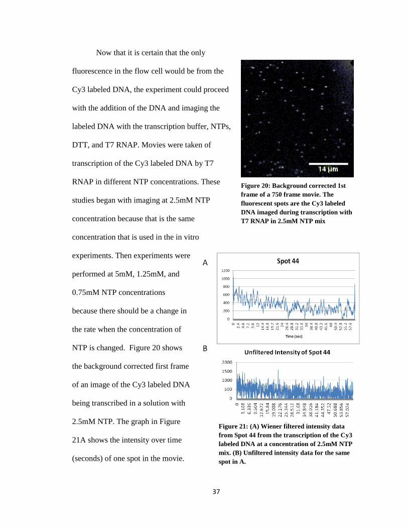
fluorescent product. Also the mix had ATP, CTP,

GTP, and UTP all together, which by itself,

would not be expected to cause fluorescence, but

an additive could have been added to increase the

stability of the solution. New ATP, CTP, GTP,

and UTP were ordered from Invitrogen. They

were mixed immediately before being imaged in

a clean flow cell and no fluorescence was seen.

The DTT, NTPs, transcription buffer, and T7 RNAP were flowed into a flow cell and

imaged again. This time no fluorescence was seen as shown in Figure 19.

Figure 18: Image of a clean glass flow

cell loaded with 2.5mM NTP mix.

Many fluorescent spots from the NTP

mix can be seen in this sample.

Figure 19: Image of clean glass flow

cell with 0.5x transcription buffer,

2.5mM NTPs, 1mM DTT, and 0.01mM

Trolox. No fluorescence was seen in

this image.

37

Now that it is certain that the only

fluorescence in the flow cell would be from the

Cy3 labeled DNA, the experiment could proceed

with the addition of the DNA and imaging the

labeled DNA with the transcription buffer, NTPs,

DTT, and T7 RNAP. Movies were taken of

transcription of the Cy3 labeled DNA by T7

RNAP in different NTP concentrations. These

studies began with imaging at 2.5mM NTP

concentration because that is the same

concentration that is used in the in vitro

experiments. Then experiments were

performed at 5mM, 1.25mM, and

0.75mM NTP concentrations

because there should be a change in

the rate when the concentration of

NTP is changed. Figure 20 shows

the background corrected first frame

of an image of the Cy3 labeled DNA

being transcribed in a solution with

2.5mM NTP. The graph in Figure

21A shows the intensity over time

(seconds) of one spot in the movie.

Figure 21: (A) Wiener filtered intensity data

from Spot 44 from the transcription of the Cy3

labeled DNA at a concentration of 2.5mM NTP

mix. (B) Unfiltered intensity data for the same

spot in A.

Figure 20: Background corrected 1st

frame of a 750 frame movie. The

fluorescent spots are the Cy3 labeled

DNA imaged during transcription with

T7 RNAP in 2.5mM NTP mix

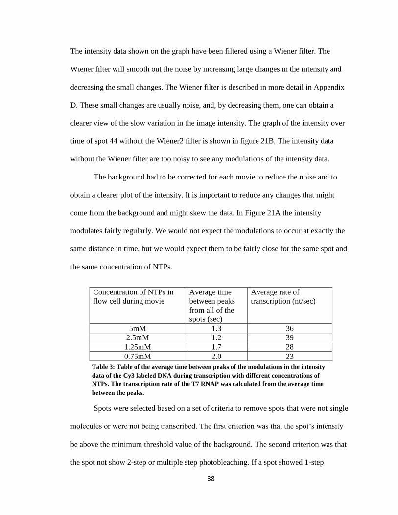
38

The intensity data shown on the graph have been filtered using a Wiener filter. The

Wiener filter will smooth out the noise by increasing large changes in the intensity and

decreasing the small changes. The Wiener filter is described in more detail in Appendix

D. These small changes are usually noise, and, by decreasing them, one can obtain a

clearer view of the slow variation in the image intensity. The graph of the intensity over

time of spot 44 without the Wiener2 filter is shown in figure 21B. The intensity data

without the Wiener filter are too noisy to see any modulations of the intensity data.

The background had to be corrected for each movie to reduce the noise and to

obtain a clearer plot of the intensity. It is important to reduce any changes that might

come from the background and might skew the data. In Figure 21A the intensity

modulates fairly regularly. We would not expect the modulations to occur at exactly the

same distance in time, but we would expect them to be fairly close for the same spot and

the same concentration of NTPs.

Spots were selected based on a set of criteria to remove spots that were not single

molecules or were not being transcribed. The first criterion was that the spot’s intensity

be above the minimum threshold value of the background. The second criterion was that

the spot not show 2-step or multiple step photobleaching. If a spot showed 1-step

Concentration of NTPs in

flow cell during movie

Average time

between peaks

from all of the

spots (sec)

Average rate of

transcription (nt/sec)

5mM 1.3 36

2.5mM 1.2 39

1.25mM 1.7 28

0.75mM 2.0 23

Table 3: Table of the average time between peaks of the modulations in the intensity

data of the Cy3 labeled DNA during transcription with different concentrations of

NTPs. The transcription rate of the T7 RNAP was calculated from the average time

between the peaks.

39

photobleaching, it proved that the spot was a single molecule. The next criterion is that

the intensity has a value of no more than 2000. The majority of the single molecules had

intensities between 500 and 1200. The last criterion was that the spot has modulations

with increases that are at least 40% higher than the baseline of the spot’s intensity. This

criterion ensured that the spot is the DNA during transcription by T7 RNAP.

Multiple spots were analyzed for each concentration of NTP and the average time

per each modulation was found. From the average time between modulations, the

transcription rate for each NTP concentration was determined. The average time between

modulations for each of the four NTP concentrations and the resulting transcription rate

are shown in Table 3. The average time between modulations for the transcription

reaction with 5mM NTP concentration was 1.268 seconds, for the 2.5mM NTP

concentration reaction the average time was 1.174 seconds, the average time for the

1.25mM NTP concentration was 1.713 seconds, and the average time for the 0.75mM

concentration was 2.036 seconds.

The time between modulations for the 2.5mM and the 5mM was the same within

error, but the 1.25mM was less than the 2.5mM or 5mM. The transcription with the

0.75mM concentration had even more time between the modulations than the 1.25mM

concentration. 2.5mM of NTP is probably at the saturation level of the reaction, so, in

order to see a change, we would need to lower the concentration. The average

transcription rate for each sample with the different NTP concentration was determined.

The experiments were begun with a NTP concentration of 2.5mM because that

was the concentration that is used for the in vitro transcription. However, this amount of

NTP is probably saturating the reaction because, in the in vitro reactions, one wants the

40

most RNA made in the least amount of time. One of the objectives of these single

molecule experiments is to determine the relationship between a change in the

concentration of NTPs and a change in the rate of transcription. In order to observe this

relationship, the NTP concentration must be reduced below the saturation point. As there

was a significant increase in the time between the modulations for the 1.25mM

concentration of NTP compared to the 2.5mM concentration, more transcription

experiments were run in lower concentrations of NTP. Samples with an NTP

concentration of 0.125mM, 0.25mM and 0.50mM were imaged, and the time between

frames was determined for these concentrations as well.

Table 4 shows the time between the peaks of the modulations in intensity for the

three lower NTP concentrations. The transcription reaction with 0.5mM NTP

concentration had an average time between peaks of 2.103 seconds, which equals a

transcription rate of 21.76nt/sec. The transcription reaction with 0.25mM NTP

concentration had an average time between peaks of 19.91nt/sec, which equals a

transcription rate of 19.91. Last, the transcription reaction with 0.125mM NTP

concentration had an average time between peaks of 2.483 seconds and a transcription

rate of 18.83nt/sec.

Concentration of NTPs in

flow cell during

experiment

Average time between

peaks from all of the spots

(sec)

Average rate of

transcription (nt/sec)

0.5mM 2.1 22

0.25mM 2.4 20

0.125mM 2.5 19 Table 4: List of time between peaks of modulations and the corresponding transcription rate for

transcription with three different NTP concentrations.

41

The average rates of transcriptions are close to the published rates for T7 RNAP

using other single molecule fluorescence techniques. For a NTP concentration of 0.2mM,

the published rate using single molecule fluorescence imaging was 42 ±8 nt/sec, which is

within 15nt/sec of rate shown in Table 4 for transcription with 0.25mM NTP

concentration. Another single molecule fluorescence technique records the T7 RNAP

transcription rate between 20 and 60 nt/sec depending on the sequence. The transcription

rates that are calculated from the modulations are close to what others are finding.

The time between the peaks of the modulations increases as the concentration of

NTPs decrease, which was expected.

This increase in time between peaks

represents a decrease in the

transcription rate as the concentration

of NTPs decreases. Because there are

less NTPs around, it takes longer for

an NTP to be attached to the growing

RNA chain by the T7 RNAP. The

decrease in rate is not steady. The

decrease between NTP concentrations

of 1.25mM and 0.75mM was more

pronounced than the decrease between

NTP concentrations 0.5mM and

0.25mM.

Figure 22: (A) Graph of the intensity over time of

Wiener filtered spot in transcription with 2.5mM

NTP concentration. (B) Graph of the intensity over

time of Wiener filtered spot in transcription with

0.125mM NTP concentration. The peaks in graph A

are much closer together than the peaks in graph B.

A

B

42

Figure 22A shows a spot from a movie of the transcription with 2.5mM NTP

concentration and Figure 22B shows a spot from a movie of transcription with 0.125mM

NTP concentration. The peaks in the graph that had the 0.125mM NTP concentration

were much more spread out than the peaks in the graph from 2.5mM NTP concentration.

Even from a quick glance, the change in transcription rate can be seen.

So far we have only compared the average transcription rate of the T7 RNAP at

the different concentrations. To realize the full use of single molecule techniques, we

want to look at the rates for each T7 RNAP transcribing a circle at a known NTP

concentration. By looking at individual polymerases, one can see the range of

transcription rates at a given NTP concentration.

Histograms of all of the times between the peaks of the modulations for the

different spots in the movies at each NTP concentration were made. These histograms

show the distribution of the rates of the individual T7 RNAP molecules with different

concentrations of NTPs. Figure 23 shows the histogram plots for each of the

concentrations of NTPs. There is a large spread in rates for each of the NTP

concentrations, but the overall spread is shifted to the right as the concentration of NTPs

decreases as shown by the average.

The x-axis scales for all of the histograms are the same so one can see how the

time between peaks changes with different concentrations of NTP. The histogram for the

transcription with 5mM and 2.5mM NTP concentration are very similar; the highest peak

was at 1.008 and 0.864 respectively. The highest peaks for both of these concentrations

are clustered around 1 second. The similarity of the histograms of transcription with

43

5mM and the 2.5mM NTP concentration agreed with the averaged time between the

peaks data.

The peaks in the histogram of transcription with 1.25mM NTP concentration were

shifted to the right compared to the histogram of the time between peaks of transcription

at 2.5mM and 5mM NTP concentrations. The majority of the peaks was clustered around

1.008 and 1.44 seconds. The peaks in the histogram of transcription with 0.75mM NTP

concentration were shifted even more to the right compared to the histogram of the time

between peaks of transcription at 1.25mM NTP concentration. The majority of the peaks

was between 0.96 and 1.872 seconds. There were relatively more peaks in the three and

four second area than were seen in any of the transcription reactions with a higher NTP

concentration.

The most common range of peaks for transcription with 0.5mM NTP

concentration was similar to the range for the transcription reactions with 0.75mM NTP

concentrations but still shifted to the right. The range for transcription with 0.5mM NTP

concentration was 1.104 to 2.064 seconds. The difference in the time between the peaks

for these two concentrations is not as large because the difference between the

concentrations is smaller. Most of the other concentrations were decreased by half, but

from 0.75mM to 0.5mM only decreased by 1/3.

The histogram showing the time between the peaks of transcription with 0.25mM

NTP concentration had most of the peaks between 1.2 and 2.448 seconds. This range is

shifted to the right of transcription with 0.5mM NTP concentration. There are also more

cycles with times between three and four seconds than in any of the transcription

reactions with higher NTP concentrations.

44

The lowest concentration of NTPs in the transcription reaction tested was

0.125mM . The peaks in the histogram for this concentration were shifted to the right

compared to transcription with 0.25mM NTP concentration. The majority of the peaks

was between 1.104 and 2.736 seconds. Transcription at this concentration also had more

times between four and five seconds than any other concentration of NTPs. There is a

wide range of times between peaks for each of the NTP concentrations. Single molecule

experiments always have a range of values because, unlike ensemble experiments, there

is no inherent averaging. Each selected spot is a labeled DNA molecule where a certain

T7 RNA polymerase is transcribing. The difference in the time between the peak of each

modulation shows the time it took for one T7 RNAP to transcribe a circle one time from

inserted Cy3 molecule to inserted Cy3 molecule.

The histograms showing the individual time between peaks for each spot for

transcription at all of the NTP concentrations tested agreed with the averaged data. Both

the histograms and the average time between peaks for each NTP concentration showed

an increasing time between peaks as the concentration of NTPs decreased.

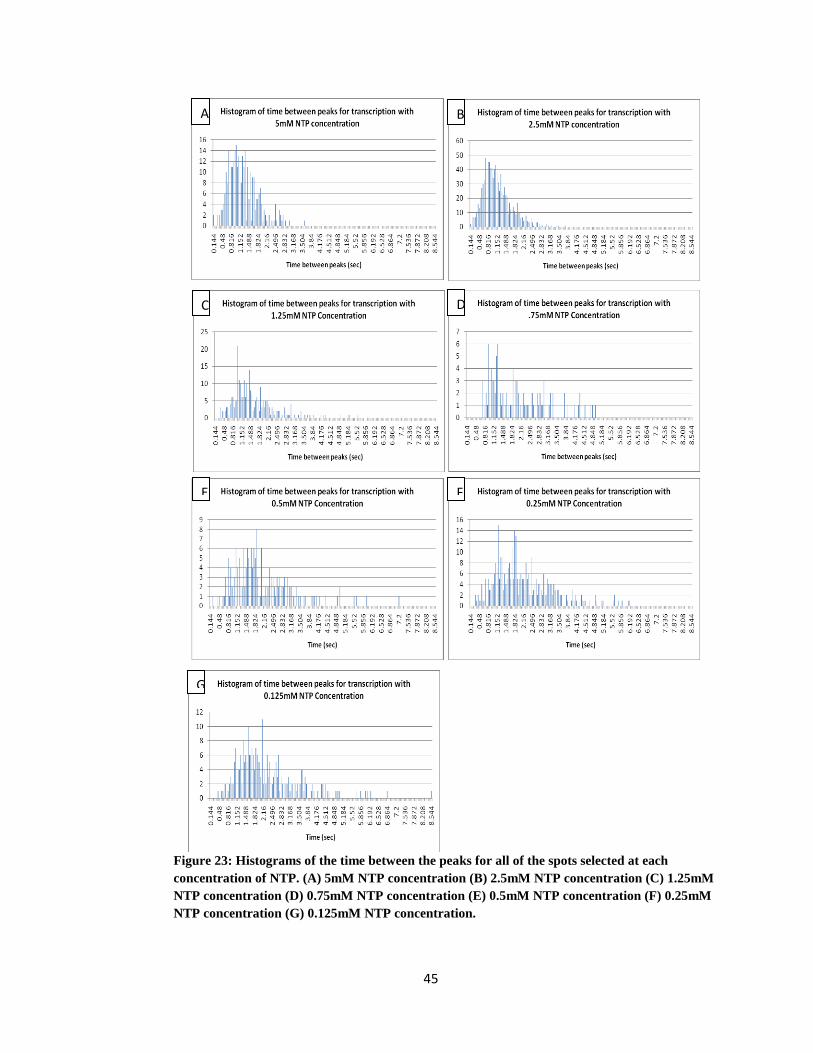
45

Figure 23: Histograms of the time between the peaks for all of the spots selected at each

concentration of NTP. (A) 5mM NTP concentration (B) 2.5mM NTP concentration (C) 1.25mM

NTP concentration (D) 0.75mM NTP concentration (E) 0.5mM NTP concentration (F) 0.25mM

NTP concentration (G) 0.125mM NTP concentration.

A B

C D

E F

G

46

BSA Coated Flowcell

The T7 RNAP transcribed the labeled DNA in the clean glass flow cell. The

modulations of the intensity were recorded and graphed. Then the transcription rate was

determined from the time between the peaks of the modulations. It has been shown that

the efficiency of an enzyme is decreased when it is on a glass surface. Even though the

reaction is done in buffer, the

polymerase could be on the glass

surface. To determine if the glass

was, in fact, decreasing the

efficiency of the enzyme, the glass

was coated with BSA.

The BSA-coated flow cell

was imaged using the

fluorescence microscope. The

coated flow cell was imaged to

make sure that there would not be

background fluorescence that

would be too bright to see the

single molecules. There was a lot of background fluorescence due to the BSA, mainly in

clumps that could be seen in the red channel and the green channel of the optical splitter.

The buffer was thought to be causing the fluorescence, so the PEM-80 buffer was

irradiated with UV light to remove any fluorescence. Then a new BSA solution was made

in the UV treated PEM-80.

Figure 24: (A) Fluorescent Optosplit image of BSA

coated flowcell rinsed with UV-treated PEM-80 buffer.

(B) Fluorescent Optosplit image of BSA coated flow

cell rinsed with 0.5x transcription buffer with 0.5mM

NTP, 1mM DTT, and 0.01mM Trolox.

47

A new clean flow cell was coated with BSA and rinsed with the UV treated PEM-

80 buffer. The flow cell was imaged using the fluorescent microscope, and the first frame

of the 200 frame movie is shown in figure 24A. There was still a significant amount of

fluorescence clustered in groups around the slide. As the PEM-80 buffer had been

irradiated to remove any fluorescence, the fluorescence must be coming from the BSA.

The flow cell was rinsed with 0.5x transcription buffer with 0.5mM NTPs, 1mM DTT,

and 1mM Trolox then imaged again (Figure 24B). The flow cell was rinsed with the

transcription buffer mixture that is used in the transcription reaction. After the rinse there

was less fluorescence, but there was still too much to see the single molecules. The BSA

was causing too much background fluorescence to use it for the single molecule

experiments, so alternative molecules to coat the glass so that the RNAP would not rest

directly on the glass surface were sought.

Poly-L-lysine coated flow cell

Because the BSA was too

fluorescent in the flow cell, in the

next set of experiments poly-L-

lysine was used to coat the cell.

The poly-L-lysine coated flow cell

was imaged using the fluorescence

microscope with the optical splitter.

A 200 frame 512x256 pixel movie was taken of the poly-L-lysine coated flow cell. The

flow cell was imaged to be certain that the poly-L-lysine on the glass was not fluorescent.

Figure 25 shows the first frame of the poly-L-lysine coated flow cell movie. No

Figure 25: Fluorescent Optosplit image of poly-L-lysine

coated flow cell.

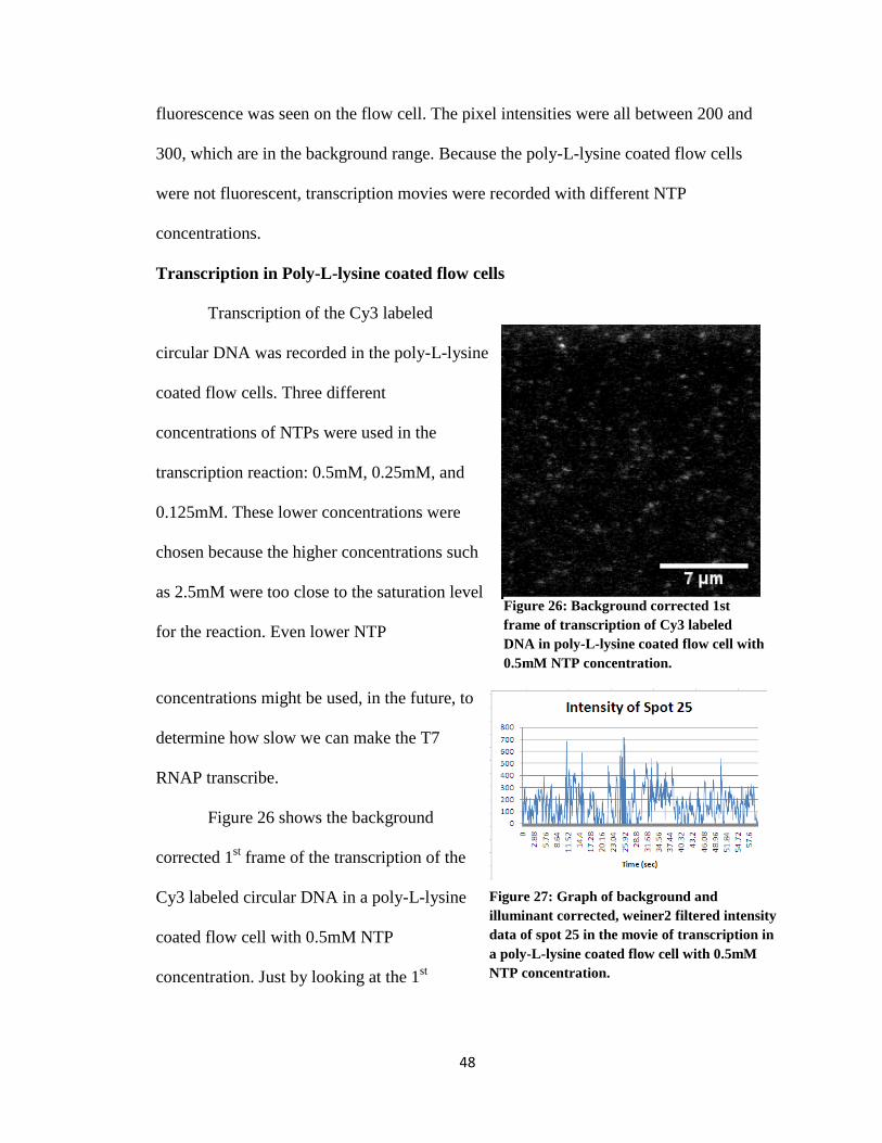
48

fluorescence was seen on the flow cell. The pixel intensities were all between 200 and

300, which are in the background range. Because the poly-L-lysine coated flow cells

were not fluorescent, transcription movies were recorded with different NTP

concentrations.

Transcription in Poly-L-lysine coated flow cells

Transcription of the Cy3 labeled

circular DNA was recorded in the poly-L-lysine

coated flow cells. Three different

concentrations of NTPs were used in the

transcription reaction: 0.5mM, 0.25mM, and

0.125mM. These lower concentrations were

chosen because the higher concentrations such

as 2.5mM were too close to the saturation level

for the reaction. Even lower NTP

concentrations might be used, in the future, to

determine how slow we can make the T7

RNAP transcribe.

Figure 26 shows the background

corrected 1st frame of the transcription of the

Cy3 labeled circular DNA in a poly-L-lysine

coated flow cell with 0.5mM NTP

concentration. Just by looking at the 1st

Figure 26: Background corrected 1st

frame of transcription of Cy3 labeled

DNA in poly-L-lysine coated flow cell with

0.5mM NTP concentration.

Figure 27: Graph of background and

illuminant corrected, weiner2 filtered intensity

data of spot 25 in the movie of transcription in

a poly-L-lysine coated flow cell with 0.5mM

NTP concentration.

49

frame, no difference can be seen from the uncoated glass flow cell. Figure 27 shows a

graph of the weiner2 filtered data for one of the spots.

The time between the peaks of the modulations was calculated for the selected

spots for each NTP concentration. From the time between peaks, the transcription rate

was determined. The time between the peaks and the transcription rates are shown in

Table 5. The transcription with 0.5mM NTP concentration has an average time between

peaks of 1.799 seconds, which equals transcription rate of 25.66 nt/sec. The transcription

with the 0.25mM NTP concentration has a time between peaks of 2.254 seconds and an

average rate of transcription of 20.83 nt/sec. The 0.125mM NTP transcription has an

average time between peaks of 3.033

seconds and a transcription rate of 15.24nt/sec.

The transcription rates of the T7 RNAP in the poly-L-lysine coated flow cell are

higher than the uncoated glass flow cell for the 0.5mM and 0.25mM NTP concentrations,

which agrees with the hypothesis that the glass was decreasing the efficiency of the T7

RNAP. For the 0.125mM NTP concentration, the transcription rate of the poly-L-lysine

coated flow cell was lower than the uncoated glass. More experiments will have to be

Concentration of NTPs in

flow cell during experiment

Average time between

peaks from all of the spots

(sec)

Average rate of

transcription (nt/sec)

0.5mM 1.8 26

0.25mM 2.3 21

0.125mM 3.0 15

Table 5: Average time between peaks of modulations and the corresponding

transcription rate for poly-L-lysine coated flow cell at different NTP concentrations.

50

done to determine why this is happening; however, one possibility is that the PLL coating

is binding some of the NTPs so that, once the concentration of NTPs is below a certain

threshold, there is a drastic decrease in the amount of available NTPs in solution.

Histograms of the time between the peaks for all of the spots for transcription in

poly-L-lysine coated flow cells for each of the different NTP concentrations were

graphed and are shown in Figure 28. The histogram of transcription with 0.5mM NTP

concentration had most of the peaks between 1.104 and 2.208 seconds. The histogram of

transcription with 0.25mM NTP concentration has most of the peaks between 1.152 and

2.304 seconds. The range of peaks for the transcription experiment with 0.25mM NTP

concentration was shifted to the right compared to the 0.5mM NTP concentration

experiment.

The histogram of transcription with 0.125mM NTP concentration had most of the

peaks between 1.344 and 3.168 seconds. This range is again shifted to the right compared

to the transcription experiments with higher NTP concentrations. The increase in the

majority of the times between the peaks of the modulations agrees with the averaged time

between the peak data. Both show that the time between the peaks increases as the NTP

concentration decreases.

Next we compared the ranges of the most common times between the peaks in the

experiments using an uncoated glass flow cell versus a poly-L-lysine coated glass flow

cell. The range of the most common time between peaks at 0.5mM NTP concentration

was 1.104 to 2.064 seconds for the uncoated glass flow cell and 1.104 and 2.208 seconds

for the poly-L-lysine coated flow cell. The ranges for both of these are very similar. The

poly-L-lysine coated flow cell had a range 0.2seconds longer. The differences in the

51

ranges of the times between the peaks of the modulations were not as pronounced as the

differences between the averaged time between peaks between the poly-L-lysine coated

and uncoated flow cell.

The most common ranges from the movies of transcription with 0.25mM NTP

concentration in an uncoated flow cell were 1.2 to 2.448 seconds and in a poly-L-lysine

coated flow cell were 1.152 and 2.304 seconds. Similar to the 0.5mM NTP concentration

movies, the range was very close to the same for both. The experiment ran in the poly-L-

lysine coated flow cell was only less than a tenth of a second faster than the experiment

in the uncoated flow cell.

There was a large difference in comparing the transcription experiments with

0.125mM NTP. The experiment with the uncoated flow cell has a range of 1.104 and

2.736 seconds, and the experiment with the poly-L-lysine coated flow cell has a range of

1.344 and 3.168 seconds. The poly-L-lysine coated flow cell had a longer time between

Figure 28: Histograms of the times between the peaks of the modulations in the movies of

transcription in poly-L-lysine coated flow cells at various concentrations. (A) 0.5mM NTP (B)

0.25mM NTP (C) 0.125mM NTP

A

C

B

52

the peaks by 0.2 to 0.4 seconds. This outcome agrees with the averaged time between

peaks, in which the average time for the uncoated experiment was 2.483 seconds and the

average time for the poly-L-lysine coated flow cell was 3.033 seconds. In both the

averaged time between peaks and the histogram of the time between peaks for the

experiments in a poly-L-lysine coated flow cell with 0.125mM NTP, the time was longer

for the experiment with the poly-L-lysine coated flow cell.

The histograms of the individual times give us a different way at looking at the

rate of the T7 RNAP. The general trends are the same for the averaged data and the single

data plotted in a histogram; the transcription rate of the T7 RNAP decreases as the NTP

concentration decreases. The histogram shows how long each T7 RNAP molecule takes

to transcribe the circle once. We can see that there are outliers; sometimes the T7 RNAP

transcribes the DNA quickly, less than a second, and sometimes it transcribes it very

slowly (or pauses) over 5 seconds. But most of the time the polymerases work at a fairly

regular and consistent pace depending on their environment.

Control Experiment

To prove that the modulations in the intensity of

the fluorescent spots were due to the proximity to Cy3 of

the polymerase during transcription and not something that

is inherent to Cy3 or due to the microscope, a negative

control experiment was done. A clean poly-L-lysine

coated flow cell was loaded with the transcription buffer,

T7 RNAP, DTT, Trolox and the labeled circular DNA, and

then imaged under the fluorescence microscope. Figure 29

Figure 29: Background

corrected 1st frame of negative

control for transcription

experiment.

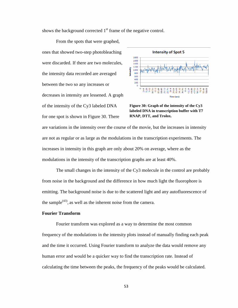
53

shows the background corrected 1st frame of the negative control.

From the spots that were graphed,

ones that showed two-step photobleaching

were discarded. If there are two molecules,

the intensity data recorded are averaged

between the two so any increases or

decreases in intensity are lessened. A graph

of the intensity of the Cy3 labeled DNA

for one spot is shown in Figure 30. There

are variations in the intensity over the course of the movie, but the increases in intensity

are not as regular or as large as the modulations in the transcription experiments. The

increases in intensity in this graph are only about 20% on average, where as the

modulations in the intensity of the transcription graphs are at least 40%.

The small changes in the intensity of the Cy3 molecule in the control are probably

from noise in the background and the difference in how much light the fluorophore is

emitting. The background noise is due to the scattered light and any autofluorescence of

the sample(43)

, as well as the inherent noise from the camera.

Fourier Transform

Fourier transform was explored as a way to determine the most common

frequency of the modulations in the intensity plots instead of manually finding each peak

and the time it occurred. Using Fourier transform to analyze the data would remove any

human error and would be a quicker way to find the transcription rate. Instead of

calculating the time between the peaks, the frequency of the peaks would be calculated.

Figure 30: Graph of the intensity of the Cy3

labeled DNA in transcription buffer with T7

RNAP, DTT, and Trolox.

54

From the frequency, the time and then the rate could be determined. A fast fourier

transform was added to the code in the

Matlab script, and a power spectrum was

graphed with the most frequent instances

over frequencies. An example of one of

the power spectra for a spot in a movie is

shown in Figure 31. No peak stands out as

the dominant frequency for three potential reasons: the noise is too high due to the

modulations not being regular enough, there are not enough data points in the fourier

transform for there to be a strong peak, or because the DC component (the distance of the

baseline of the data from the x-axis) of the intensity data is too large. The latter of the two

possibilities may be remedied, but there is nothing one can do if the modulations from the

Cy3 molecule are not regular.

To try to get a better signal to noise ratio, longer movies movies were recorded.

The number of frames was increased from 1250 to 2000. This approach did not help

because increasing the number of frames also increased the time between frames, and by

the end of the 2000 frames there were usually none or only one or 2 fluorophores still

active. The increase of the time between frames was due to a computer issue.

Next an attempt was made to obtain a better signal to noise ratio by removing the

DC component in the graphs of the intensity. This method would eliminate the empty

space in the graph where the intensities, even in the low troughs, are above zero. The

power spectrum of a spot with its DC component removed is shown in Figure 32, which

is from the same data that was used in Figure 31. As you can see, the signal to noise ratio

Figure 31: Power spectrum of weiner2

filtered intensity data.

55

in the DC component removed spot is better

than the signal to noise in the regular power

spectrum, but the signal is still less than double

the size of some of the noise.

The power spectrum cannot be used to

determine the frequency of the modulations as

long as the signal to noise ratio is low. Another algorithm will have to be found that can

determine the most common frequencies allowing for the quasi-periodic state of the

modulations

Conclusions

Cy3 was determined to be a good probe for the single molecule fluorescence

analysis of the transcription rate of T7 RNA polymerase. The fluorescent molecule was

bright enough to be seen in the single molecule level with short exposure time, and it was

stable enough to stay active long enough for the movies of transcription to be recorded.

The photochemical half-life of the Cy3 labeled circular DNA was 23.5 seconds and many

lasted for over a minute. The Cy3 also made a good probe because it did not inhibit the

circularization of the linear DNA or the transcription of the circular DNA it was a part of.

The sensitivity of Cy3 to its environment and its availability were the main

reasons it was chosen as the probe. The intensity of the Cy3 molecule increases by at

least 40% when it was in the T7 RNAP. Once it was outside of the RNAP, the intensity

of the RNAP decreased to baseline levels. These modulations were used to determine the

transcription rate of T7 RNAP. All of the transcription experiments were done at 22°C

Figure 32: Power spectrum of weiner2

filtered intensity data with DC component

removed.

56

with 3mM Mg+2

concentration. For the 2.5mM NTP concentration, the transcription rate

was 39nt/sec; for the 1.25mM NTP concentration, the transcription rate was 28nt/sec; for

the 0.75mM NTP concentration, the transcription rate was 23nt/sec; for the 0.5mM NTP

concentration, the transcription rate was 22nt/sec; for the 0.25mM NTP concentration, the

transcription rate was 20nt/sec, and for the 0.125mM NTP concentration, the NTP

concentration was 19nt/sec. The transcription rate was shown to decrease as the NTP

concentration decreased, showing a correlation between the modulations and what the

polymerase was doing.

The coating of the flow cell with poly-L-lysine changed the transcription rates,

but the same overall decrease in transcription rate as the NTP concentration decreased

was seen. The experiment with 0.5mM NTP concentration had a transcription rate of

22nt/sec; for the 0.25mM NTP concentration, the transcription rate was 20nt/sec, and for

the 0.125mM NTP concentration, the transcription rate was 19nt/sec. Single molecule

fluorescence imaging can be used to determine the rate of a RNA polymerase using

rolling circle transcription.

57

Appendix A

45nt DNA circle

The 45nt DNA has a sequence of 5’-CTG GAG GAG ATT TTG TGG TAT CGA TTC

GTC TCT TAG AGG AAG CTA-3’.

The 45nt DNA with the Cy3 internal modification has a sequence of 5’-CTG GAG GAG

ATT TTG TGG TA(Cy3)T CGA TTC GTC TCT TAG AGG AAG CTA-3’.

The only difference between the two is the addition of the Cy3 molecule between bases

20 and 21. Below is a scale representation from Spartan 08 version 1.2.0 that shows the

T7 RNAP (left) and the circular DNA (right). The size of the DNA circle is similar in

size to the T7 RNAP.

58

Appendix B

Secondary Structure of 45nt DNA circle

Using Mfold free software, the most energy favorable secondary structure for the DNA

circle in buffer is shown below. About two thirds of the DNA is a circle, but one-third of

the bases form a hairpin. The Cy3 molecule is not shown in the image below, but it

would be between bases 20 and 21. Because the Cy3 would be in the circular part of the

DNA, it would not change the secondary structure much from what is shown here.

59

Appendix C

Ethanol Precipitation Protocol

1. Aliquot DNA so that no more than 100μL of DNA is in a 1.5mL microcentrifuge

tube

2. Add 1mL 99.9% ethanol and 15μL of 2mM NaCl to each tube with DNA

3. Place in a -80ºC freezer for 45 minutes

4. Centrifuge at 12,500 rpm at 4ºC for 15 minutes

5. Decant ethanol solution

6. Wash the pellet to remove salt by adding 500μL of 70% ethanol to the tubes,

briefly vortex and then centrifuge at 4°C for 10 minutes

7. Decant ethanol

8. Remove remaining ethanol with vacuum centrifuge

9. A DNA pellet should remain

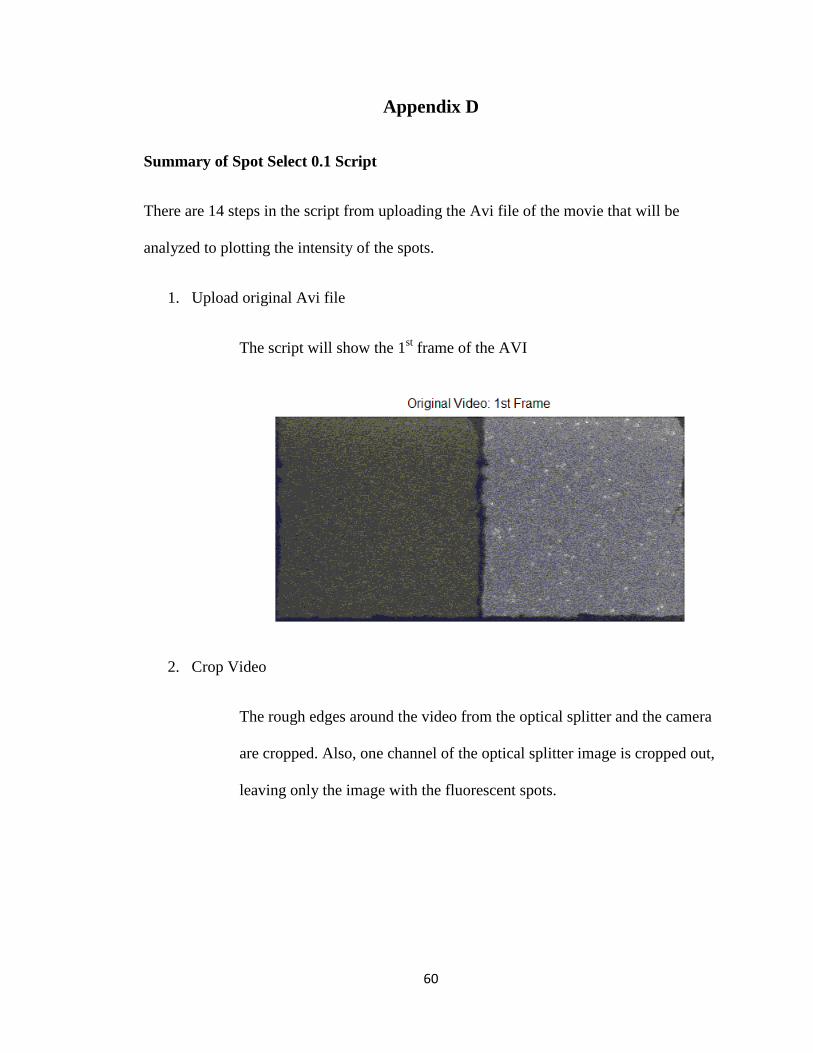
60

Appendix D

Summary of Spot Select 0.1 Script

There are 14 steps in the script from uploading the Avi file of the movie that will be

analyzed to plotting the intensity of the spots.

1. Upload original Avi file

The script will show the 1st frame of the AVI

2. Crop Video

The rough edges around the video from the optical splitter and the camera

are cropped. Also, one channel of the optical splitter image is cropped out,

leaving only the image with the fluorescent spots.

61

3. Histogram of the intensity values of the pixels

This gives a histogram of all of the pixel values in the 1st 50 frames of the

movie

4. Maxima of each pixel

62

A 10 frame moving average filter is applied to the pixels of the 1st 50

frames of the movie. An image is formed that shows the maximum

intensity value of each pixel in the 1st 50 frames.

5. Background calculated from the maxima

The background of the movie is assumed to be smooth. The image of the

maxima of each pixel is shrunk to 1/10 its size. The shrunken image is

then recreated by substituting each pixel with the lowest pixel value in a

3x3 pixel region around the pixel of interest. The image is blurred to

smooth out the background, and then the image is increased back to

normal size. The resulting image is the background calculated from the

maxima.

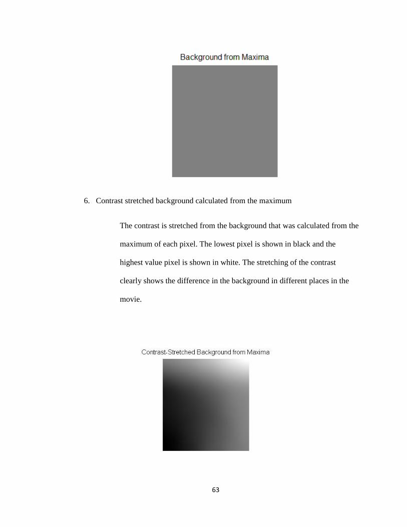
63

6. Contrast stretched background calculated from the maximum

The contrast is stretched from the background that was calculated from the

maximum of each pixel. The lowest pixel is shown in black and the

highest value pixel is shown in white. The stretching of the contrast

clearly shows the difference in the background in different places in the

movie.

64

7. Background corrected maximum

The background image is subtracted from the maxima image and any

negatives are changed to 0 since intensity cannot be negative. The pixel

values are normalized, so, instead of the range being from 0-255, it is now

0-1.

8. Binarized spots

From the background corrected maxima image, any pixel that is greater

than the threshold value is considered a potential spot and any pixel less

than the threshold value is considered background. The threshold is

chosen by the user; it is a percentage of pixel intensity value. For these

experiments I used a pixel intensity of 0.3, so any pixels that are more

intense than 30% of the pixels in the movie are potential spots. Any

grouping of 8 or more pixels above the threshold is considered a spot and

is given a value of 1. Any groupings of less than 8 pixels above the

65

threshold or any pixels below the threshold are given a value of 0 and are

considered background. To use this algorithm in Matlab there is a choice

between 4 or 8 pixels. 8 was chosen because it was assumed that the light

from any fluorphore would illuminate at least 7 surrounding pixels.

9. Background mask

This image is made from the binarized image. Each spot from the last

image is given a value of 0. A 15 pixel circle around each spot is also

given a value of 0. Every other pixel in the image is given a value of 1.

This creates a mask of only the background pixels. This background is

used later in the script for the illuminant correction.

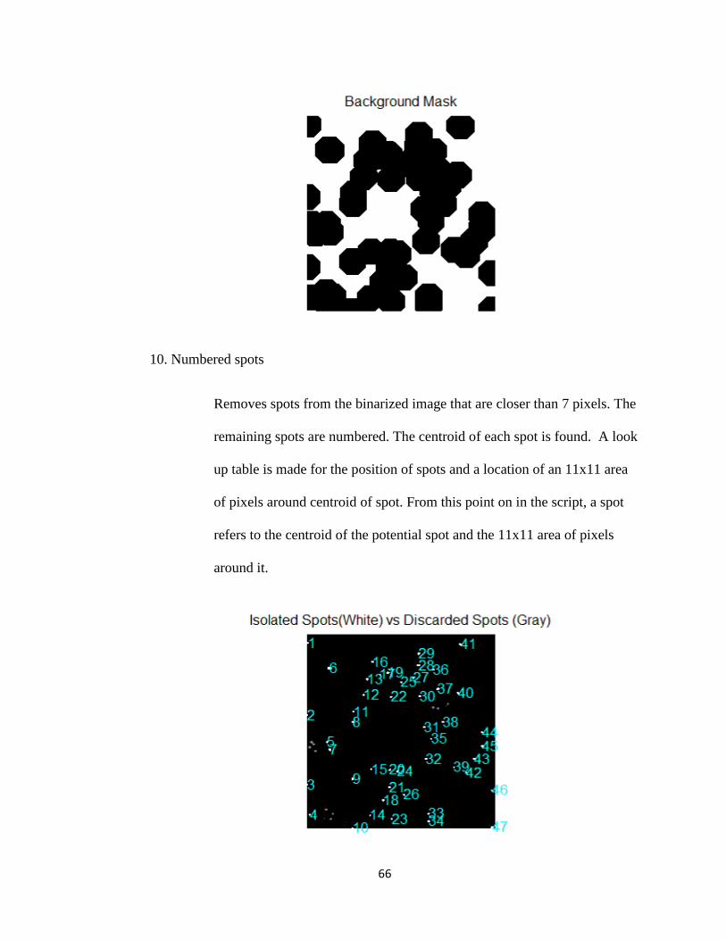
66

10. Numbered spots

Removes spots from the binarized image that are closer than 7 pixels. The

remaining spots are numbered. The centroid of each spot is found. A look

up table is made for the position of spots and a location of an 11x11 area

of pixels around centroid of spot. From this point on in the script, a spot

refers to the centroid of the potential spot and the 11x11 area of pixels

around it.

67

11. Mean Background

The mean value of all pixels over all frames is calculated and an image is

formed. The background of the movie is again assumed to be smooth. The

image of the mean of each pixel is shrunk to 1/10 its size. The shrunken

image is then recreated by substituting each pixel with the lowest pixel

value in a 3x3 pixel region around the pixel of interest. The image is

blurred to smooth out the background, and then the image is increased

back to normal size. This image is the calculated background from the

mean. The background from the mean is used as the background that is

subtracted when looking at the intensities of individual spots.

12. Mean contrast background

The contrast is stretched from the background that was calculated from the

mean of each pixel. The lowest pixel is shown in black and the highest

value pixel is shown in white. The stretching of the contrast shows clearly

shows the difference in the background in different places in the movie.

68

13. Graph of illuminant strength

Shows the change of the illuminance over time during the movie. The

illuminance is calculated by taking the average of all of the pixels in the

background for each frame. The background mask was used to determine

which pixels were part of the background. This number is graphed for

each frame of the movie.

69

14. Plot intensity data of the spots

Intensity data for each spot is plotted over time.

i. Original- The intensities of each spot (11x11 pixel area) are

summed and these are the intensity value for each spot at each

frame. The intensity values are from the original cropped video.

These values are graphed over time either in frames or seconds.

ii. Background corrected- The mean background is subtracted from

each frame of the cropped movie giving the background corrected

video. The intensities of each spot (11x11 pixel area) are summed

and these are the intensity values for each spot at each frame.

These values are graphed over time either in frames or seconds.

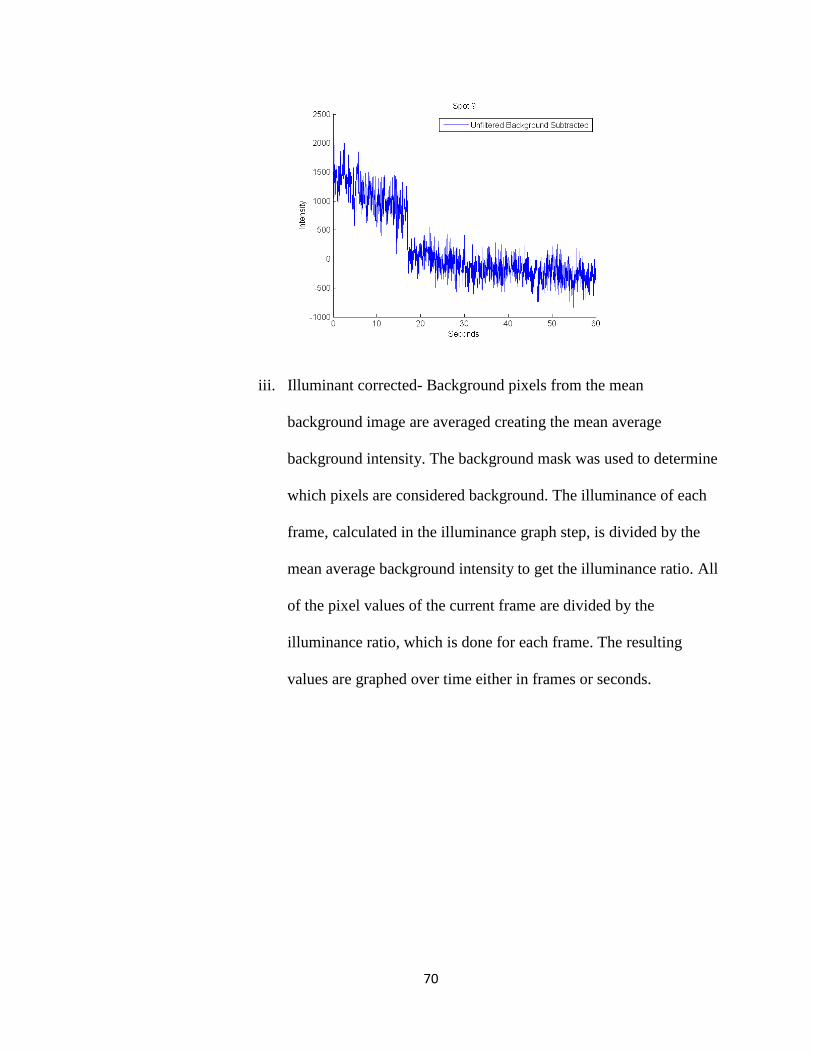
70

iii. Illuminant corrected- Background pixels from the mean

background image are averaged creating the mean average

background intensity. The background mask was used to determine

which pixels are considered background. The illuminance of each

frame, calculated in the illuminance graph step, is divided by the

mean average background intensity to get the illuminance ratio. All

of the pixel values of the current frame are divided by the

illuminance ratio, which is done for each frame. The resulting

values are graphed over time either in frames or seconds.

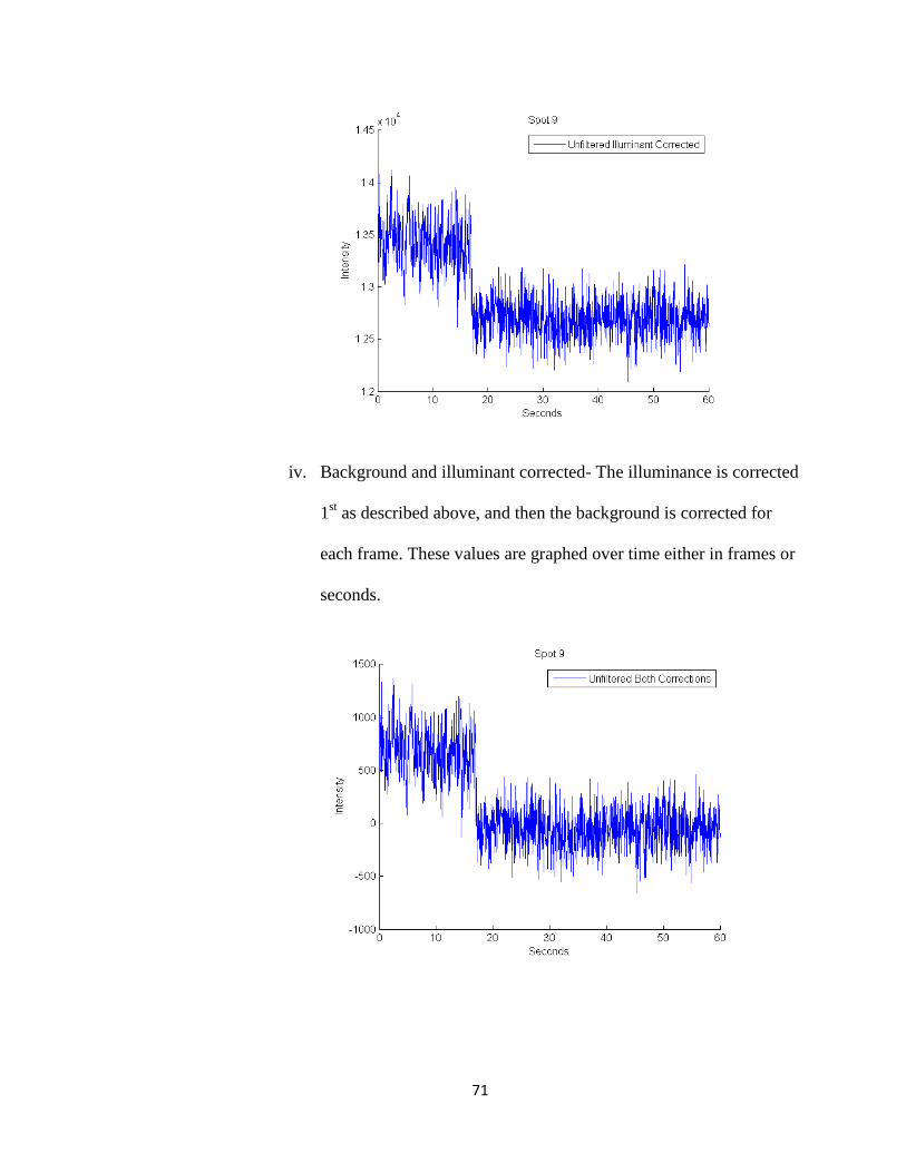
71

iv. Background and illuminant corrected- The illuminance is corrected

1st as described above, and then the background is corrected for

each frame. These values are graphed over time either in frames or

seconds.

72

v. Wiener filter- A 10 frame wiener filter can be applied to any of the

above plot data. The wiener filter smoothes out some of the noise

from the data using the following algorithm

[Equation 3]

Where v2 is the average of all of the local estimated variances, μ is

the local mean around each frame, and σ2 is the local variance

around each frame, a is the value of the frame of interest. These

values are graphed over time either in frames or seconds.

73

Appendix E

SpotSelect 0.1 code

classdef StateNav < hgsetget properties CurrentStep = Step() CurrentState FunctionsBack FunctionsForward StateNames = ... { 'Start', 'Video Loaded', 'Video Cropped', 'Histogram',

'Maxima', 'Maxima Background', ... 'Maxima Contrast Background', 'Maxima Corrected',

'Binarized Spots', 'Background Mask', ... 'Labeled Spots', 'Mean Background', 'Mean Contrast

Background', 'Illuminant Strength', ... 'Plots' } StatesCount end methods function Obj = StateNav() Obj.FunctionsForward = ... { @Obj.LoadVideo, @Obj.CropVideo, @Obj.CreateHistogram,

@Obj.FindMaxima, @Obj.FindMaximaBackground, ... @Obj.ShowMaximaContrastBackground, @Obj.CorrectMaxima,

@Obj.Binarize, ... @Obj.CreateBackgroundMask, @Obj.FilterSpots,

@Obj.CreateSpotsLUT, ... @Obj.ShowMeanContrastBackground, @Obj.CreatePlotData

@Obj.ShowPlots }; Obj.FunctionsBack = ... { @Obj.UnLoadVideo, @Obj.UnCropVideo,

@Obj.UnCreateHistogram, @Obj.UnFindMaxima, @Obj.UnFindMaximaBackground,

... @Obj.UnShowMaximaContrastBackground,

@Obj.UnCorrectMaxima, @Obj.UnBinarize, ... @Obj.UnCreateBackgroundMask, @Obj.UnFilterSpots,

@Obj.UnCreateSpotsLUT, ... @Obj.UnShowMeanContrastBackground,

@Obj.UnCreatePlotData @Obj.UnShowPlots }; Obj.StatesCount = length(Obj.StateNames); Obj.CurrentState = State(1, Obj.StateNames{1}); Obj.CurrentStep.StateStart = Obj.CurrentState;

74

Obj.CurrentStep.StateCurrent = Obj.CurrentState; Obj.CurrentStep.StateEnd = Obj.CurrentState; end

function [Video Plot] = Forward(Obj, Video, Plot, States) % Set States for Current Step Obj.CurrentStep.StateStart = Obj.CurrentState; Obj.CurrentStep.StateCurrent = Obj.CurrentStep.StateStart; Obj.CurrentStep.StateEnd.Number =

Obj.CurrentStep.StateStart.Number + States;

% Coerce End State to Be In Range if Obj.CurrentStep.StateEnd.Number > Obj.StatesCount; Obj.CurrentStep.StateEnd.Number = Obj.StatesCount; end Obj.CurrentStep.StateEnd.Name =

Obj.StateNames{Obj.CurrentStep.StateEnd.Number};

% If State Change if Obj.CurrentStep.StateStart.Number <

Obj.CurrentStep.StateEnd.Number % For Each State Change for StateCurrent = Obj.CurrentStep.StateStart.Number :

Obj.CurrentStep.StateEnd.Number - 1 Obj.CurrentStep.Function =

Obj.FunctionsForward{StateCurrent}; [Video Plot] = Obj.CurrentStep.Function(Video,

Plot); Obj.CurrentStep.StateCurrent.Number = StateCurrent

+ 1; Obj.CurrentStep.StateCurrent.Name =

Obj.StateNames{Obj.CurrentStep.StateCurrent.Number}; end Obj.CurrentState = Obj.CurrentStep.StateEnd; end end

function [Video Plot] = Back(Obj, Video, Plot, States) % Set States for Current Step Obj.CurrentStep.StateStart = Obj.CurrentState; Obj.CurrentStep.StateCurrent = Obj.CurrentStep.StateStart; Obj.CurrentStep.StateEnd.Number =

Obj.CurrentStep.StateStart.Number - States;

% Coerce End State to Be In Range if Obj.CurrentStep.StateEnd.Number < 1; Obj.CurrentStep.StateEnd.Number = 1; end Obj.CurrentStep.StateEnd.Name =

Obj.StateNames{Obj.CurrentStep.StateEnd.Number};

% If State Change

75

if Obj.CurrentStep.StateStart.Number >

Obj.CurrentStep.StateEnd.Number % For Each State Change for StateCurrent = Obj.CurrentStep.StateStart.Number :

-1 : Obj.CurrentStep.StateEnd.Number + 1 Obj.CurrentStep.Function =

Obj.FunctionsBack{StateCurrent - 1}; [Video Plot] = Obj.CurrentStep.Function(Video,

Plot); Obj.CurrentStep.StateCurrent.Number = StateCurrent

- 1; Obj.CurrentStep.StateCurrent.Name =

Obj.StateNames{Obj.CurrentStep.StateCurrent.Number}; end

Obj.CurrentState = Obj.CurrentStep.StateEnd; end end

function Change(stateName)

end

% 2 Video Loaded -> 1 Start function [Video Plot] = UnLoadVideo(Obj, Video, Plot) close; Video = rmfield(Video, 'Video'); end

function ShowOriginalVideo1stFrame(Obj, Video) imshow(Video.Video(:, :, 1)); title('Original Video: 1st Frame'); end

function [Video Plot] = LoadVideo(Obj, Video, Plot) aviDesc = 'AVI Video Files (*.avi)'; [file, path, ~] = uigetfile({'*.avi', aviDesc},'Load

Video'); mmObj = mmreader([path file]); avi = read(mmObj); Video.Video = squeeze(avi(:, :, 1, :)); Obj.ShowOriginalVideo1stFrame(Video); end

function [Video Plot] = UnCropVideo(Obj, Video, Plot) Video = rmfield(Video, 'VideoCropped'); Obj.ShowOriginalVideo1stFrame(Video); end

function ShowCroppedVideo(Obj, Video) imshow(Video.VideoCropped(:, :, 1)); title('Cropped Video: 1st Frame'); end

function [Video Plot] = CropVideo(Obj, Video, Plot)

76

% Need update for uniform crop if Video.Crop.Uniform == true Video.Crop.Left = Video.Crop.Top; Video.Crop.Right = Video.Crop.Top; Video.Crop.Bottom = Video.Crop.Top; end vidWid = size(Video.Video, 2); vidHt = size(Video.Video, 1); vidTop = Video.Crop.Top + 1; vidBot = vidHt - Video.Crop.Bottom; vidRight = vidWid - Video.Crop.Right; if Video.Optosplit == false vidLeft = Video.Crop.Left + 1; else vidLeft = vidWid / 2 + Video.Crop.Left + 1; end Video.VideoCropped = Video.Video(vidTop:vidBot,

vidLeft:vidRight, :); Obj.ShowCroppedVideo(Video); end

function [Video Plot] = UnCreateHistogram(Obj, Video, Plot) Video = rmfield(Video, 'Histogram'); Obj.ShowCroppedVideo(Video); end

function ShowHistogram(Obj, Video) bar(Video.Histogram); axis tight; title('Histogram of Frames 1-50'); xlabel('Intensity'); ylabel('Number of Pixels'); end

function [Video Plot] = CreateHistogram(Obj, Video, Plot) Video.Histogram = zeros(256, 50); for FrameNum = 1:50 Video.Histogram(:, FrameNum) =

imhist(Video.VideoCropped(:,:,FrameNum)); end Video.Histogram = sum(Video.Histogram, 2); %Video.Histogram = Video.Histogram; Obj.ShowHistogram(Video); end

function [Video Plot] = UnFindMaxima(Obj, Video, Plot) Video = rmfield(Video, 'Maxima'); Obj.ShowHistogram(Video); end

function ShowMaxima(Obj, Video) imgCur = Video.Maxima ./ max(Video.Maxima(:)); imshow(imgCur); title('Pixel Maxima'); end

77

function [Video Plot] = FindMaxima(Obj, Video, Plot) tempAvg = convn(Video.VideoCropped(:, :, 1:50),

ones(1,1,10)/10, 'valid'); Video.Maxima = max(tempAvg,[],3); Obj.ShowMaxima(Video); end

function [Video Plot] = UnFindMaximaBackground(Obj, Video,

Plot) Video = rmfield(Video, 'MaximaBackground'); Obj.ShowMaxima(Video); end

function ShowMaximaBackground(Obj, Video) % background with 0 = black, 255 = white imshow(Video.MaximaBackground,[0 255]); title('Background from Maxima'); end

function [Video Plot] = FindMaximaBackground(Obj, Video, Plot) bgs = imopen(imresize(Video.Maxima, 0.1), strel('square',

3)); filter = imfilter(bgs, fspecial('disk', 5), 'replicate'); Video.MaximaBackground = imresize(filter,

size(Video.Maxima)); Obj.ShowMaximaBackground(Video); end

function [Video Plot] = UnShowMaximaContrastBackground(Obj,

Video, Plot) Obj.ShowMaximaBackground(Video); end

function [Video Plot] = ShowMaximaContrastBackground(Obj,

Video, Plot) % background with minval = black, maxval = white imshow(Video.MaximaBackground,[]); title('Contrast-Stretched Background from Maxima'); end

function [Video Plot] = UnCorrectMaxima(Obj, Video, Plot) Video = rmfield(Video, 'MaximaCorrected'); [Video Plot] = Obj.ShowMaximaContrastBackground(Video,

Plot); end

function ShowCorrectedMaxima(Obj, Video) imshow(Video.MaximaCorrected); title({'Maxima', '(Background-Subtracted & Rescaled)'}); end

function [Video Plot] = CorrectMaxima(Obj, Video, Plot) Video.MaximaCorrected = Video.Maxima -

Video.MaximaBackground; Video.MaximaCorrected(Video.MaximaCorrected < 0) = 0;

78

Video.MaximaCorrected = Video.MaximaCorrected ./

max(Video.MaximaCorrected(:)); Obj.ShowCorrectedMaxima(Video); end

function [Video Plot] = UnBinarize(Obj, Video, Plot) Video = rmfield(Video, 'SpotsBinarized'); Obj.ShowCorrectedMaxima(Video); end

function ShowBinarizedSpots(Obj, Video) imshow(Video.SpotsBinarized); title('Binarized Spots'); end

function [Video Plot] = Binarize(Obj, Video, Plot) Video.SpotsBinarized = Video.MaximaCorrected >

Video.PixelThreshold; Video.SpotsBinarizedLabeled = bwlabel(Video.SpotsBinarized,

8); Obj.ShowBinarizedSpots(Video); end

function [Video Plot] = UnCreateBackgroundMask(Obj, Video,

Plot) Video = rmfield(Video, 'BackgroundMask'); Obj.ShowBinarizedSpots(Video); end

function ShowBackgroundMask(Obj, Video) imshow(Video.BackgroundMask); title('Background Mask'); end

function [Video Plot] = CreateBackgroundMask(Obj, Video, Plot) Video.BackgroundMask = Video.MaximaCorrected <

Video.PixelThreshold; % leave a very large 15 pixel margin around spots Video.BackgroundMask = imerode(Video.BackgroundMask,

strel('disk', 15)); Obj.ShowBackgroundMask(Video); end

function [Video Plot] = UnFilterSpots(Obj, Video, Plot) Video = rmfield(Video, 'SpotProperties'); Obj.ShowBackgroundMask(Video); end

function ShowLabeledSpots(Obj, Video) imshow(double(Video.SpotsBinarizedLabeled > 0) +

double(Video.L2 > 0),[]); for i = 1 : length(Video.SpotProperties) LabelX = Video.SpotProperties(i).Centroid(1); LabelY = Video.SpotProperties(i).Centroid(2); text(LabelX, LabelY, num2str(i), 'Color', 'cyan');

79

end title('Isolated Spots(White) vs Discarded Spots (Gray)'); end

function [Video Plot] = FilterSpots(Obj, Video, Plot) SpotDistanceMinimum = 7; Video.L2 =

uint16(zeros(size(Video.SpotsBinarizedLabeled))); for i = 1 : max(Video.SpotsBinarizedLabeled(:)) SpotsDilated = imdilate(Video.SpotsBinarizedLabeled ==

i, strel('disk', SpotDistanceMinimum)); if ~any(SpotsDilated & Video.SpotsBinarizedLabeled ~= 0

& Video.SpotsBinarizedLabeled ~= i) Video.L2(Video.SpotsBinarizedLabeled == i) = i; end end Video.SpotProperties = regionprops(Video.L2, 'Centroid',

'Area'); Video.SpotProperties([Video.SpotProperties.Area] == 0) =

[]; Obj.ShowLabeledSpots(Video); end

function [Video Plot] = UnCreateSpotsLUT(Obj, Video, Plot) Video = rmfield(Video, {'SpotsLUT' 'Mean'

'MeanBackground'}); Obj.ShowLabeledSpots(Video); end

function ShowMeanBackground(Obj, Video) imshow(Video.MeanBackground, [0 255]); title('Background from Mean'); end

function [Video Plot] = CreateSpotsLUT(Obj, Video, Plot) % first prepare lookup table to copy frame pixels to

appropriate spot ... ssize = 11; % insert an odd number here Video.SpotsLUT = zeros(ssize, ssize,

length(Video.SpotProperties)); for i = 1 : length(Video.SpotProperties) % create array of ssize rows around the row of each

spot r = round(Video.SpotProperties(i).Centroid(2)) - (ssize

- 1) / 2 : round(Video.SpotProperties(i).Centroid(2)) + (ssize-1) / 2; c = round(Video.SpotProperties(i).Centroid(1)) - (ssize

- 1) / 2 : round(Video.SpotProperties(i).Centroid(1)) + (ssize-1) / 2; r(r < 1) = 1; r(r > size(Video.VideoCropped, 1)) =

size(Video.VideoCropped, 1); %avoid rows outside of image c(c < 1) = 1; c(c > size(Video.VideoCropped, 2)) =

size(Video.VideoCropped, 2); %avoid cols outside of image [C R] = meshgrid(c, r); Video.SpotsLUT(:,:,i) =

sub2ind(size(Video.VideoCropped), R, C);

80

end

Video.Mean = mean(Video.VideoCropped, 3); bgs = imopen(imresize(Video.Mean, 0.1), strel('square',

3)); Video.MeanBackground = imresize(imfilter(bgs,

fspecial('disk',5), 'replicate'), size(Video.Mean)); Obj.ShowMeanBackground(Video); end

function [Video Plot] = UnShowMeanContrastBackground(Obj,

Video, Plot) Obj.ShowMeanBackground(Video); end

function [Video Plot] = ShowMeanContrastBackground(Obj, Video,

Plot) imshow(Video.MeanBackground, []); title('Contrast-Stretched Background from Mean'); end

function [Video Plot] = UnCreatePlotData(Obj, Video, Plot) Video = rmfield(Video, 'Frames'); Plot = rmfield(Plot, {'Illuminant', 'Data'}); [Video Plot] = Obj.ShowMeanContrastBackground(Video, Plot); end

function ShowIlluminantStrength(Obj, Plot) plot(Plot.Illuminant); axis auto; %axis([0 500 -0.1 1.2]); legend('Illuminant Strength'); title('Illuminant Strength vs Time'); ylabel('Illuminant Strength (1 = Average)'); xlabel('Time'); end

function [Video Plot] = CreatePlotData(Obj, Video, Plot) Video.Frames = size(Video.VideoCropped, 3); BGIll = mean(Video.MeanBackground(Video.BackgroundMask)); Plot.Illuminant = zeros(1, Video.Frames); SpotsQty = size(Video.SpotsLUT, 3); Spots = zeros(11, 11, SpotsQty, Video.Frames, 4);

for FrameCurrent = 1:Video.Frames Frame(:, :, 1) = double(Video.VideoCropped(:, :,

FrameCurrent)); FrameThis = Frame(:, :, 1); Frame(:, :, 2) = FrameThis - Video.MeanBackground; FrameIlluminance =

mean(FrameThis(Video.BackgroundMask)); Plot.Illuminant(FrameCurrent) = FrameIlluminance /

BGIll; Frame(:, :, 3) = FrameThis /

Plot.Illuminant(FrameCurrent);

81

Frame(:, :, 4) = Frame(:, :, 3) - Video.MeanBackground;

for PlotType = 1:4 PlotTypeFrame = Frame(:, :, PlotType); Spots(:, :, :, FrameCurrent, PlotType) =

PlotTypeFrame(Video.SpotsLUT); end end

SpotsRowSum = sum(Spots, 1); clear Spots; SpotsColSum = sum(SpotsRowSum, 2); clear SpotsRowSum; Plot.Data = zeros(SpotsQty, Video.Frames, 8); Plot.Data(:, :, 1:4) = squeeze(SpotsColSum); clear SpotsColSum;

% Wiener2 for PlotType = 1:4 PlotOrig = Plot.Data(:, :, PlotType); [PlotW2 ~] = wiener2(PlotOrig, [1 10]); Plot.Data(:, :, PlotType + 4) = PlotW2; end

% Plot graph of computed illuminant strength Obj.ShowIlluminantStrength(Plot); end

function [Video Plot] = UnShowPlots(Obj, Video, Plot) Obj.ShowIlluminantStrength(Plot); end

function [Video Plot] = ShowPlots(Obj, Video, Plot) Plot = UpdatePlots(Plot); end

function [Video Plot] = UnDoSomething(Obj, Video, Plot)

end

function ShowSomething(Obj, Video)

end

function [Video Plot] = DoSomething(Obj, Video, Plot)

end

end end

82

References

1. (2010) Nucleobase. Wikipedia Commons,

http://en.wikipedia.org/wiki/Nucleobase

2. Champe, P.C., Harvey, R.A., Ferrier, D.R. (2008). Biochemistry 4th

Edition.

Lippincott Williams & Wilkins. 417-418.

3. Cheetham, G.M.T., & Steitz, T.A. (1999). Structure of a Transcribing T7

RNA Polymerase Initiation Complex. Science, 286, Retrieved April 9, 2008,

from http://www.sciencemag.org

4. Cramer, P., Bushnell, D.A., Fu, J., Gnatt, A.L., Maier-Davis, B., &

Thompson, N.E., Burgess, R.R., Edwards, A.M., David, P.R., Kornberg, R.D.

(2000). Architecture of RNA Polymerase II and Implications for the

Transcription Mechanism. Science, 228, 640-649.

5. Daubendick, S.L., Ryan, K., Kool, E.T. (1995). Rolling circle RNA synthesis:

Circular Oligonucleotides as efficient substrates for T7 RNA polymerase.

JACS. 117 (29), 7818-7819.

6. Daubendick, S. L., & Kool, E. T. (1997). Generation of catalytic RNAs by

rolling circle transcription of synthetic DNA nanocircles. Nature

Biotechnology. 15, 273-277.

7. Seyhan, A. A., Vlassov, A. V., & Johnston, B. H. (2006). RNA interferece

from multimeric shRNAs generated by rolling circle transcription.

Oligonucleotides. 16, 353-363.

8. Furukawa, K., et al. (2008). Fluorescence generation from tandem repeats of a

malachite green RNA aptamer using rolling circle transcription. Bioinorganic

and Medicinal Chemistry Letters, 18, 4562-4565.

9. (2010). Protein Data Bank. http://www.rcsb.org/pdb/home/home.do

10. Durniak, K.J., Bailey, S., Steitz, T.A. (2008). The structure of a transcribing

T7 RNA polymerase in transition from initiation to elongation. Science, 322,

553-557.

11. Tahirov, T.H., Temiakov, D., Anikin, M., Patlan, V., McAllister, W.T., et. al.

(2002). Structure of a T7 RNA polymerase elongation complex at 2.9Å

resolution. Nature, 420, 43-50.

12. Thomen, P., Lopez, P.J., Heslot, F. (2005). Unraveling the mechanism of

RNA-polymerase forward motion by using mechanical force. Physical Review

Letters. 94(12) 128102-128105.

13. Lyakhov, D.L., He, B., Zhang, X., Studier, F.W., Dunn, J.J., McAllister, W.T.

(1998). Pausing and termination by bacteriophage T7 RNA polymerase. J Mol

Biol. 280(2), 201-213.

14. Branch, A.D., Robertson, H.D. (1984). A replication cycle for viroids and

other small infectious RNA’s. Science, 223, 450-455.

15. Symons, R.H. (1997). Plant pathogenic RNAs and RNA catalysis. Nucleic

Acids Research, 25(14), 2683-2689.

83

16. Macnaughton, T.B., Shi, S.T., Modahl, L.E., Lai, M.C. (2002) Rolling circle

replication of hepatitis delta virus RNA is carried out by two different cellular

RNA polymerases. Journal of Virology, 76, 3920-3927.

17. Daubendick, S. L., & Kool, E. T. (1997). Generation of catalytic RNAs by

rolling circle transcription of synthetic DNA nanocircles. Nature

Biotechnology. 15, 273-277.

18. Diegleman, A. M., & Kool, E. T. (1998). Generation of circular RNAs and

trans-cleaving catalytic RNAs by rolling circle transcription of circular DNA

oligonucleotides encoding hairpin ribozymes. Nucleic Acids Research. 26,

3235-3241.

19. Seyhan, A.A. (2006). Generation of ribozymes by rolling circle transcription

of promotorless single-stranded DNA circles in mammalian cells. Turkish

Journal of Biochemistry, 31, Retrieved February 18, 2009, from

http://www.turkjbiochem.com/2006/toc2006.html.

20. Orrit, M., Bernard, J. (1990). Single pentacene molecules detected by

fluorescence excitation in a p-Terphenyl crystal. Physical Review Letters, 65,

(21), 2716-2719.

21. Perkins, T.T., Quake, S.R., Smith, D.E., Chu, S. (1994). Relaxation of a single

DNA molecule observed by optical microscopy. Science, 264, 822-826.

22. Yildiz, A. et al. (2003). Myosin V walks hand-over-hand: Single fluorophore

imaging with 1.5nm localization. Science, 300 (5628) 2061-2065.

23. Rust, M.J., Bates, M., Zhuang, X. (2006). Sub-diffraction-limit imaging by

stochastic optical reconstruction microscopy (STORM). Nature Methods, 3,

793-796.

24. Betzig, E. et al. (2006). Imaging intracellular fluorescent proteins at

nanometer resolution. Science, 313, 1642-1645.

25. Roy, R., Hohng, S., Ha, T. (2008). A practical guide to single-molecule

FRET. Nature Methods, 5 (6), 507-516.

26. (2008). Total internal reflection fluorescence. TIRF Technologies,

http://www.tirftechnologies.com.

27. Axelrod, D., Davidson, M.W. (2010). Introduction and theoretical aspects.

Microscopy Resource Center,

http://www.olympusmicro.com/primer/techniques/fluorescence/tirf/tirfintro.ht

ml.

28. Axelrod, D., Davidson, M.W. (2010). Basic Microscope Configuration.

Microscopy Resource Center,

http://www.olympusmicro.com/primer/techniques/fluorescence/tirf/tirfconfigu

ration.html.

29. Luo, G., Wang, M., Konigsberg, W.H., Xie, X.S. (2007). Single-molelcule

and ensemble fluorescence assays for a functionally important conformational

change in T7 DNA polymerase. PNAS, 104(31), 12610-12615.

30. Halling, P.J. (2006). Understanding enzyme action at solid surfaces.

Biocatalysis, 34(2), 309-311.

31. Shaevitz, J.W., Abbondanzieri, E.A., Landick, R., Block, S.M. (2003).

Backtracking by single RNA polymerase molecules observed at near-base-

pair resolution. Letters to Nature, 426, 684-687.

84

32. Arnold, S. et al. (2001). Kinetic modeling and simulation of in vitro

transcription by phage T7 RNA polymerase. Biotechnology and

Bioengineering, 72(5), 548-561.

33. Yin, H., Wang, M.D., Svoboda, K., Landink, R., Block, S.M., Gelles, J.

(1995). Transcription against an applied force. Science, 270, 1653-1657.

34. Tang, G., Roy, R., Bandwar, R.P., Ha, T., Patel, S.S. (2009). Real-time

observation of the transition from initiation to elongation of the RNA

polymerase. PNAS, 106(52), 22175-22180.

35. Kim, J.H., Larson, R.G. (2007). Single-molecule anaylsis of 1D diffusion and

transcription elongation of T7 RNA polymerase along individual stretched

DNA molecules. Nucleic Acids Research, 35(11), 3848-3858.

36. Davenport, R.J., Wuite, J.L., Landick, R., Bustamante, C. (2000). Single-

molecule study of transcriptional pausing and arrest by E. coli RNA

polymerase. Science, 287, 2497-2500.

37. Gueroui, Z., Place, C., Freyssingeas, E., Berge, B. (2002). Observation by

fluorescence microscopy of transcription on single combed DNA. PNAS, 99,

(9), 6005-6010.

38. Davidson, M.W. (2010). Fundamentals of mercury arc lamps. Retrieved from

http://zeiss-campus.magnet.fsu.edu/articles/lightsources/mercuryarc.html.

39. http://www.invitrogen.com/site/us/en/home/support/Research-

Tools/Fluorescence-SpectraViewer.html?fileId1=A555Hh2o.

40. (2010). Rolera-MGi Plus Data Sheet. Q Imaging,

http://www.qimaging.com/products/cameras/scientific/rolera_mgiplus.php.

41. FlashGel system – Protocol. https://shop.lonza.com/shop/prd/flashgel-rna-

system/lonza_b2b/5.1-

6_1_75_65_8_11/2/DF369A8B4FB6E1F18852001A4B525E10/.

42. Selvin, P.R., & Ha, T. (2008). Single molecule techniques: a laboratory

manual. Cold Spring Harbor, NY: Cold Spring Harbor Laboratory Press.

43. Foldes-Papp, Z., Demel, U., Tilz, G.P. (2001). Ultrasensitive detection and

identification of fluorescent molecules by FCS: Impact for immunobiology.

PNAS, 98(20), 11509-11514.