developing a national forest productivity model - ncas technical
TRANSCRIPT

tech
nica
l rep
ort n
o. 2
3
The National Carbon Accounting System provides a complete
accounting and forecasting capability for human-induced sources and
sinks of greenhouse gas emissions from Australian land based
systems. It will provide a basis for assessing Australia’s progress
towards meeting its international emissions commitments.
http://www.greenhouse.gov.au
technical report no. 23
Developing a NationalForest Productivity Model
Jenny Kesteven,Joe Landsberg andURS Australia
Developing a National Forest Productivity M
odel
national carbonaccounting system

The National Carbon Accounting System:• Supports Australia's position in the international development of policyand guidelines on sinks activity and greenhouse gas emissionsmitigation from land based systems.
• Reduces the scientific uncertainties that surround estimates of landbased greenhouse gas emissions and sequestration in the Australian context.
• Provides monitoring capabilities for existing land based emissions andsinks, and scenario development and modelling capabilities thatsupport greenhouse gas mitigation and the sinks development agendathrough to 2012 and beyond.
• Provides the scientific and technical basis for internationalnegotiations and promotes Australia's national interests ininternational fora.
http://www.greenhouse.gov.au/ncas
For additional copies of this report phone 1300 130 606
Series 1 Publications
1. Setting the Frame
2. Estimation of Changes in Soil Carbon Due to Changes in Land Use
3. Woody Biomass: Methods for Estimating Change
4. Land Clearing 1970-1990: A Social History
5a. Review of Allometric Relationships for Estimating Woody Biomass for Queensland, the NorthernTerritory and Western Australia
5b. Review of Allometric Relationships for Estimating Woody Biomass for New South Wales, theAustralian Capital Territory, Victoria, Tasmania and South Australia
6. The Decay of Coarse Woody Debris
7. Carbon Content of Woody Roots: Revised Analysis and a Comparison with Woody ShootComponents (Revision 1)
8. Usage and Lifecycle of Wood Products
9. Land Cover Change: Specification for Remote Sensing Analysis
10. National Carbon Accounting System: Phase 1 Implementation Plan for the 1990 Baseline
11. International Review of the Implementation Plan for the 1990 Baseline (13-15 December 1999)
Series 2 Publications
12. Estimation of Pre-Clearing Soil Carbon Conditions
13. Agricultural Land Use and Management Information
14. Sampling, Measurement and Analytical Protocols for Carbon Estimation in Soil, Litter and CoarseWoody Debris
15. Carbon Conversion Factors for Historical Soil Carbon Data
16. Remote Sensing Analysis Of Land Cover Change - Pilot Testing of Techniques
17. Synthesis of Allometrics, Review of Root Biomass and Design of Future Woody BiomassSampling Strategies
18. Wood Density Phase 1 - State of Knowledge
19. Wood Density Phase 2 - Additional Sampling
20. Change in Soil Carbon Following Afforestation or Reforestation
21. System Design
22. Carbon Contents of Above-Ground Tissues of Forest and Woodland Trees
23. Developing a National Forest Productivity Model
24. Analysis of Wood Product Accounting Options for the National Carbon Accounting System
25. Review of Unpublished Biomass-Related Information: Western Australia, South Australia, NewSouth Wales and Queensland
26. CAMFor User Manual

DEVELOPING A NATIONAL FORESTPRODUCTIVITY MODEL
Jenny Kesteven+
, Joe Landsberg#
and URS Australia°
+
Centre for Resource and Environmental Studies, Australian National University, Canberra
#
Landsberg Consulting Pty Ltd°
URS Australia
National Carbon Accounting System Technical Report No. 23
May 2004

Australian Greenhouse Officeii
Printed in Australia for the Australian Greenhouse Office
© Commonwealth of Australia 2004
This work is copyright. It may be reproduced in whole or part for study or training purposessubject to the inclusion of an acknowledgement of the source and no commercial usage orsale results. Reproduction for purposes other than those listed above requires the writtenpermission of the Communications Team, Australian Greenhouse Office. Requests andenquiries concerning reproduction and rights should be addressed to the CommunicationsTeam, Australian Greenhouse Office, GPO Box 621, CANBERRA ACT 2601.
For additional copies of this document please contact the Australian Greenhouse OfficePublications Hotline on 1300 130 606.
For further information please contact the National Carbon Accounting System athttp://www.greenhouse.gov.au/ncas/
Neither the Australian Government nor the Consultants responsible for undertaking thisproject accepts liability for the accuracy of or inferences from the material contained in thispublication, or for any action as a result of any person’s or group’s interpretations,deductions, conclusions or actions in reliance on this material.
May 2004
Environment Australia Cataloguing-in-Publication
Kesteven, Jennifer L.
Developing a national forest productivity model / Jenny Kesteven, Joe Landsberg and URSAustralia.
p. cm.
(National Carbon Accounting System technical report; No. 23)
Bibliography
ISSN: 1442 6838
1. Forest productivity-Australia-Simulation methods. 2. Forest productivity-Australia-Forecasting. I. Landsberg, J.J. (Joseph John), 1938- . II. URS Australia. III. AustralianGreenhouse Office.IV. Series
333.75'0994'011-dc22

National Carbon Accounting System Technical Report iii
SUMMARYKnowledge of the spatial and temporal patterns offorest growth is fundamental to estimating thecarbon stocks (and biomass) of mature forests andrates of carbon accumulation in any forest regrowth.
As part of the National Carbon Accounting Systemdeveloped by the Australian Greenhouse Office,indices of forest growth were developed and usedto predict potential biomass at maturity (forestproductivity) and rates for biomass incrementacross the Australian continent over time.
This report documents the application of theseforest growth indices in developing a NationalForest Productivity Model.

Australian Greenhouse Officeiv
National Carbon Accounting System Technical Report v
TABLE OF CONTENTS
Page No.
Summary iii
List of Symbols and Acronyms vii
1. Introduction 1
2. Input Data 2
2.1 Soils 2
2.1.1 Soil Water Holding Capacity (SC) 2
2.1.2 Soil Nutrient Status (SN) 4
2.2 Climate 5
2.2.1 Fitting the Climate Surfaces 5
2.2.1.1 Errors in the Model 7
2.2.1.2 From Surface Coefficient Files to Maps 8
2.2.2 Digital Elevation Model (DEM) 8
2.2.3 Station Dictionary 10
2.2.4 Long-Term Average Climate Variables 11
2.2.4.1 Average Temperature 12
2.2.4.2 Number of Frost Days 12
2.2.4.3 Radiation 12
2.2.4.4 Vapour Pressure Deficit (VPD) 15
2.2.5 Monthly Average Climate Variables 15
2.2.5.1 Average Temperature 16
2.2.5.2 Maximum Temperature 17
2.2.5.3 Minimum Temperature 19
2.2.5.4 Rainfall 20
2.2.5.5 Frost Days 23
2.2.5.6 Radiation 24
2.3 Normalised Difference Vegetation Index (NDVI) 24
3. Calculation of Plant Productivity 26
3.1 Temperature Modifier 26
3.2 Frost Modifier 27
3.3 Vapour Pressure Deficit (VPD) Modifier 27
3.4 Soil Water Content (SW) 28
3.5 Absorbed Photosynthetically Active Radiation (APAR) 32
3.6 Plant Productivity Index 33
4. Select References 36
Appendix 1 – Preliminary Investigations: Spatial Estimation of Plant Productivity and Classification of Non-Commercial Vegetation Types 39

Australian Greenhouse Officevi
LIST OF FIGURESPage No.
Figure 1. Potential available soil water holding capacity (SC). 3
Figure 2. Soil nutrient status (SN). 4
Figure 3. The Australian DEM. 9
Figure 4. A screen capture for station 061121 – Lostock Post Office. 11
Figure 5. Long-term monthly average temperature. 13
Figure 6. Long-term average number of frost days per month. 14
Figure 7. Annual average temperature derived from monthly data grids for 1968-2002 and examples of low (1976), average (1982) and high (1996) temperature years. 16
Figure 8. Australian average maximum temperature (Tmax) and the 12 month running mean. 17
Figure 9. Maximum temperature grids for high and low continental average values for July and December. 18
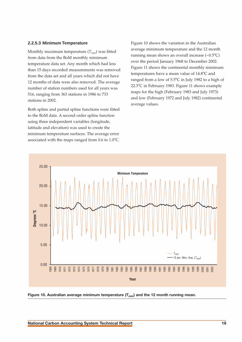
Figure 10. Australian average minimum temperature (Tmin) and the 12 month running mean. 19
Figure 11. Minimum temperature grids for high and low continental average values for July and February. 20
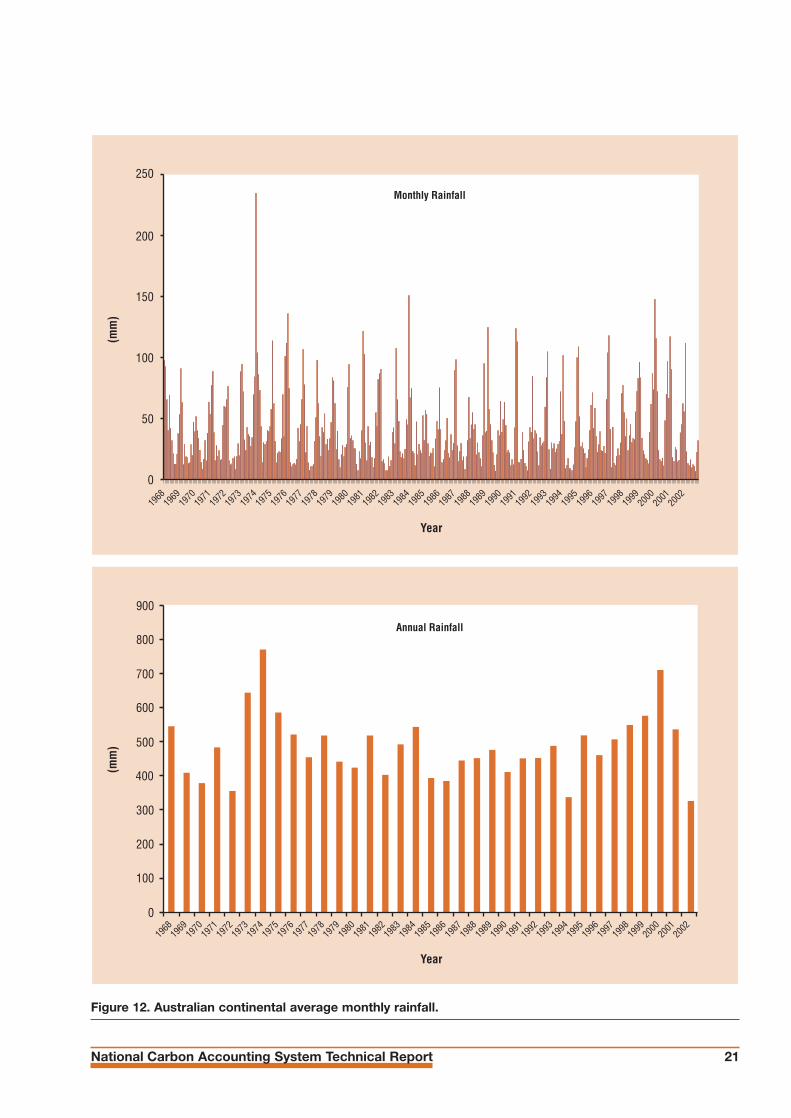
Figure 12. Australian continental average monthly rainfall. 21
Figure 13. Annual rainfall 1970–2002. 22
Figure 14. Australian continental average annual number of frost days. 23
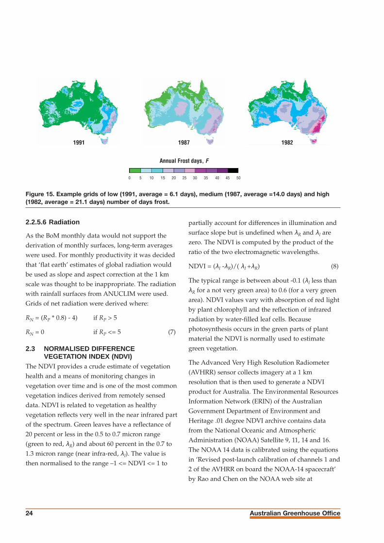
Figure 15. Example grids of low (1991, average = 6.1 days), medium (1987, average =14.0 days) and high (1982, average = 21.1 days) number of days frost. 24
Figure 16. Temperature modifier spatial equations (from Equation 11) for January and July long-term averages. 26
Figure 17. The frost modifier equation for the July long-term average. 27
Figure 18. VPD modifier spatial equations for January and July long-term averages. 28
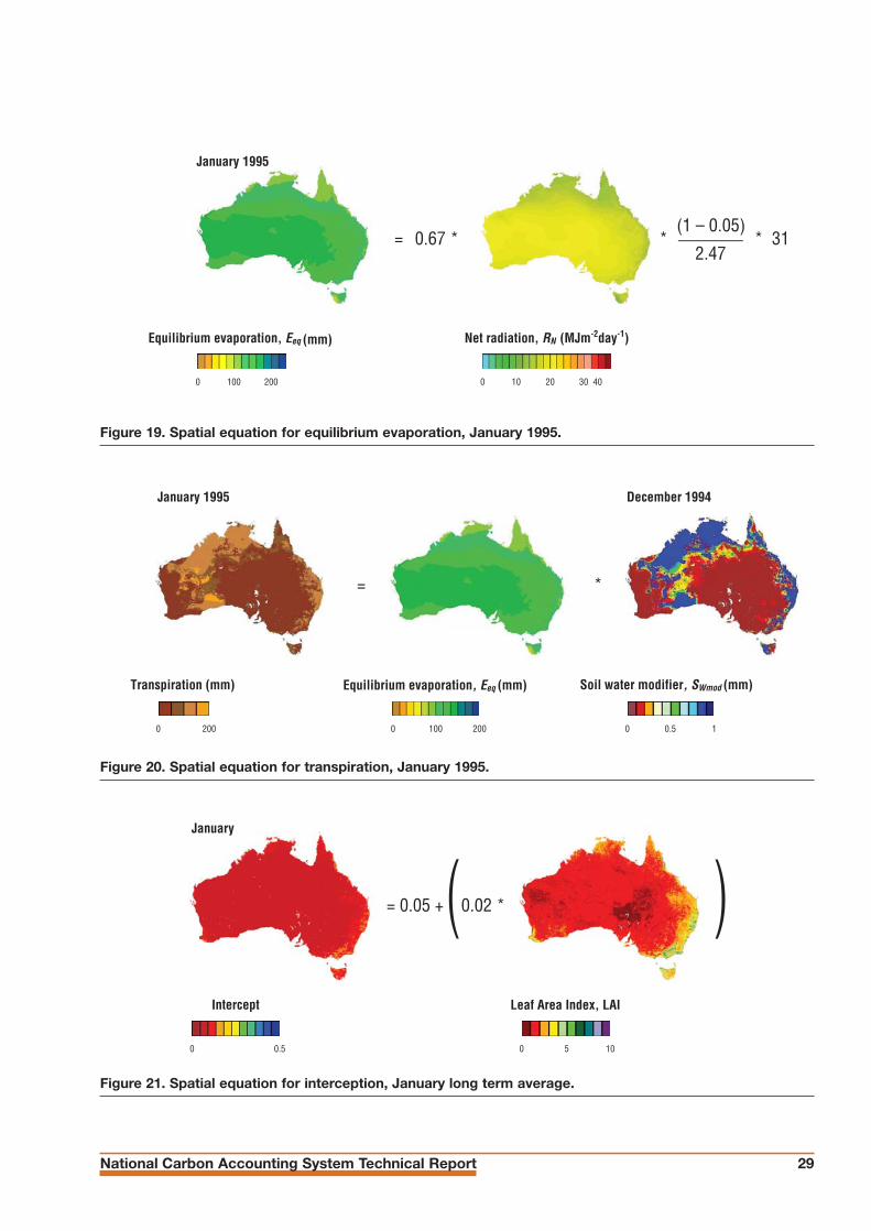
Figure 19. Spatial equation for equilibrium evaporation, January 1995. 29
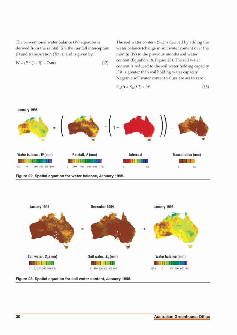
Figure 20. Spatial equation for transpiration, January 1995. 29
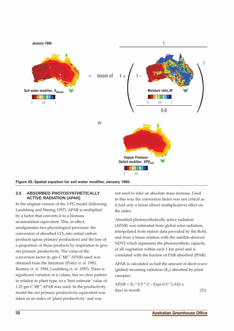
Figure 21. Spatial equation for interception, January long term average. 29
Figure 22. Spatial equation for water balance, January 1995. 30
Figure 23. Spatial equation for soil water content, January 1995. 30
Figure 24. Spatial equation for moisture ratio, January 1995. 31
Figure 25. Spatial equation for soil water modifier, January 1995. 32
Figure 26. Long-term average APAR for January and July. 33
Figure 27. Spatial equations for productivity indices, January and July long-term averages. 33
Figure 28. Derived long-term average plant productivity index for Australia. 34
Figure 29. Derived annual continental productivity indices 1970-2002. 35

National Carbon Accounting System Technical Report vii
LIST OF TABLESPage No.
Table 1 ANUCLIM variables used in the plant productivity modelling. 12
Table 2. ANUSPLIN variables created for the long-term plant productivity modelling. 12
Table 3. Monthly climate variables. 16

Australian Greenhouse Officeviii
P Rainfall (mm)
RA Adjusted direct radiation
RC Slope and aspect modified radiation
RD Direct radiation
RF Diffuse radiation
RG Global radiation
RN Net radiation (MJ m-2 day-1)
RP Radiation with rainfall
SN Soil nutrient status
SC Soil water holding capacity
SW Soil water
SWmod Soil water modifier
T Temperature (oC)
Tavg Average monthly temperature/meanair temperature (oC)
Tdew9, Tdew3 Dew point temperature (9 am and 3 pm)
Tdry9, Tdry3 Dry bulb temperature (9 am and 3 pm)
Thigh Monthly average temperature abovewhich plant growth stops
Tlow Monthly average temperature belowwhich plant growth stops
Tmax Maximum air temperature (oC)
Tmin Minimum air temperature (oC)
Tmod Temperature modifier
Topt Optimum temperature for growth
Trans Transpiration
VPD Vapour Pressure Deficit
VPDmod Vapour Pressure Deficit modifier
W Water balance
LIST OF SYMBOLS AND ACRONYMS
AGO Australian Greenhouse Office
APAR Absorbed PhotosyntheticallyActive Radiation
BoM Bureau of Meteorology (Australia)
CRES Centre for Resource andEnvironmental Studies
CSIRO Commonwealth Scientific andIndustrial Research Organization
DEM Digital Elevation Map
e°(T) Saturation vapour pressure at airtemperature T (kPa)
Eeq Equilibrium evaporation
exp(x) 2.7183 (base of natural logarithm)raised to the power x
F Frost (days per month)
Fmod Frost modifier
fPAR Fraction of Photosynthetically ActiveRadiation absorbed
GCV Generalised Cross Validation
GPP Gross Primary Productivity
I Interception intercept
J Month
LAI Leaf Area Index (m2 (leaf area) m-2
(soil surface))
M Moisture ratio
NDVI Normalised Difference Vegetation Index
λI Near infra-red electromagneticwavelengths
λR Low micron range electromagneticwavelengths
NPP Net Primary Production

National Carbon Accounting System Technical Report 1
1. INTRODUCTION
Net primary productivity (NPP) is the rate at whichchemical or solar energy is converted to biomass.The main primary producers are the green plants,which convert solar energy, carbon dioxide andwater to glucose, and eventually to plant tissue.
Estimation of productivity can be obtained throughdifferent methods. Direct measurement methodsinclude destructive sampling of the above-groundand below-ground plant biomass, and the recordingof carbon dioxide fluxes at the vegetation-atmosphere interface.
Available direct measurements of NPP have somelimitations for mapping productivity across theAustralian continent. The reliability of available datais variable – the data is limited in number and notevenly distributed among the various types ofecosystems. To overcome these deficiencies inmeasured data several model types have beendeveloped. These are either physiological modelssimulating ecosystem fluxes from environmentalvariables, remote sensing-based models interpretingthe light spectrum reflected by the land surface, orinverse models deducing fluxes from time and spacevariations in atmospheric CO2 and 13C data. Processmodels with physiological functions (i.e. those thatacknowledge temporal variability due to changingbiophysical conditions such as rainfall andtemperature) offer the opportunity to simulate pastand future changes in NPP according toenvironmental changes.
A truncated spatial version of the 3-PG (process)model (after Landsberg and Waring, 1997) wasdeveloped as part of the National CarbonAccounting System (NCAS) to predict forestproductivity across the Australian continent. Theresultant ‘productivity index’ model as documentedhere retains the essential features of biomass NPPestimation, without the biomass fixation (GrossPrimary Productivity (GPP) minus NPP) and carbonpartitioning procedures.
A relative index of plant productivity was mappedfor Australia using the ‘productivity index’ model –based on the relationship between the amount ofphotosynthetically active radiation absorbed byplant canopies (APAR) and the various productivitymodifiers that affect plant growth (e.g. temperature,soil water content, frost). The model used a monthlytime step to derive both a long-term averagemonthly productivity index (~250 m resolution) anda monthly productivity index for 1970 to 2002 (1 kmresolution).
Factors converting APAR to productivity indiceswere reduced from presumed optimum values bymodifiers dependent on soil fertility, atmosphericvapour pressure deficits, soil water content andtemperature. The ANUCLIM and ANUSPLINprograms were used to generate climate surfaces forthe continent. Soil fertility and water holdingcapacity values were obtained from the CSIROusing the digital Soil Atlas of Australia. Leaf AreaIndex, essential for the calculation of APAR, wasestimated from 10-year mean values of NormalisedDifference Vegetation Indices (NDVI), for 1 kmpixels, for the entire country. Incoming short-waveradiation – and hence APAR – was corrected forslope and aspect using a Digital Elevation Map(DEM) for the long-term average, but with 1 kmpixels being used in the monthly productivity mapsderived as this made no significant difference to theresults. Analyses were, therefore, carried out onestimates based on the assumption of flat terrain.
The resultant maps (as digital grids) of plantproductivity index, for each month for Australia,provide relative indices of plant productivity(reflecting the spatial and temporal patterns of plantgrowth) in any region. The data generated isintegral to the estimation of carbon stocks under theNCAS and provides a framework for assessingcarbon accumulation by various vegetation types.

Australian Greenhouse Office2
2. INPUT DATA
The production of mapped productivity indices forAustralia required integration and analysis of anumber of spatially represented environmentalvariables. These included: soil water holdingcapacity (to estimate water balance), soil nutrientstatus, Advanced Very High Resolution Radiometer(AVHRR) data (to estimate the NormalisedDifference Vegetative Index (NDVI)), and variousclimate variables (temperature, rainfall and numberof frost days).
2.1 SOILSThe Atlas of Australian Soils (Northcote et. al.
1960–1968) was integrated with a set of interpretedsoil variables from CSIRO (McKenzie and Hook1992) to produce continental maps of potentialavailable water holding capacity (PAWHC) andnutrient status of soils.
The Atlas of Australian Soils completed in 1968(Northcote et. al. 1960-1968) and made available indigital form in 1990 provides the only consistentsource of spatial information for the continent.While large areas have been surveyed in more detailduring the last 30 years, those surveys have not beencompiled to produce an updated continental map.
McKenzie et. al. 2000 provided a set of interpretedsoil variables (from McKenzie and Hook 1992) thatcan be used with the Digital Atlas. Theinterpretations for each soil type were based,wherever possible, on data held within the CSIRONational Soil Database. Summaries from thedatabase were used with other sources ofinformation to assign an interpreted value foreach variable.
Soil fertility and water holding capacity (SC) wereobtained by merging the Atlas of Australian soils(Northcote et. al. 1960-1968) and data provided byMcKenzie et. al. 2000. The data provided includedsoil fertility and water holding capacity for both the
dominant soil type (by area) and the average of thetop five dominant soils. McKenzie (pers. comm.)advised using the properties of the dominant soiltype (by area) to characterise the region. Caveats onthe use of the Digital Atlas of Australian Soils arepresented in McKenzie et. al. (2000).
The resultant data had limitations, as a largeproportion of soil variation within a region occurredover short distances which could not be resolved atthe mapping scale of the Atlas. The qualitativenature of the Digital Atlas and restrictions associatedwith the classification scheme and structure of thesoil-landscape model imposed further constraints.
The Atlas of Australian Soils uses 725 soil profileclasses, normally at the level of Principle ProfileForm (PPF) (e.g. Ug5.15). The legend of the Atlasdefines 3,060 map unit types. The map unit typeshave various combinations of the 725 soil profileclasses. The map unit type descriptions identifydominant and subdominant soil profile classes.Many of the map unit types occur more than onceand the Digital Atlas has 22,560 mapped polygons.
McKenzie and Hook (1992) prepared interpretationsof the 725 soil profile classes. The dominant soil ineach map unit type was identified and interpretedvalues for each soil profile class were ascribed toeach map unit type. Lookup tables were createdfrom the accompanying spreadsheets. Some soilpolygons had PPFs containing ‘Undefined’ or ‘NS’ -their soil attributes were coded so as to representno data.
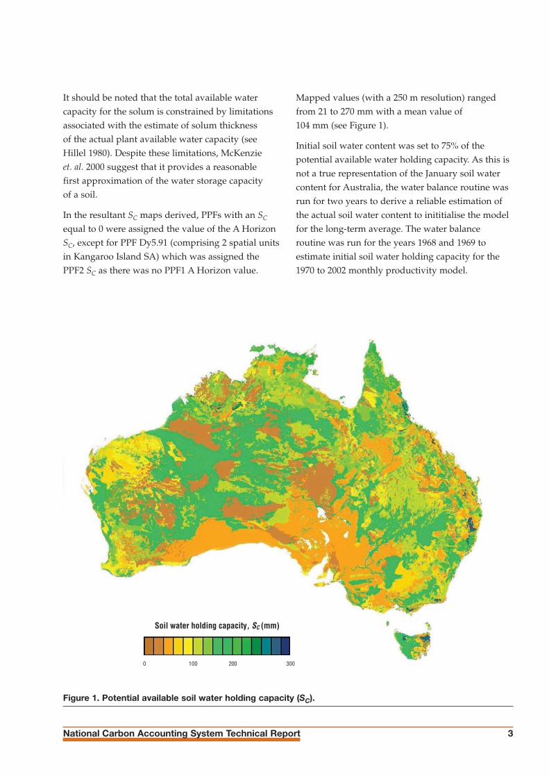
2.1.1 Soil Water Holding Capacity (SC).
Available water capacity is presented on a per unitdepth basis, as a total for each horizon, and as atotal for the solum. The total solum wasrecommended (McKenzie pers. comm.) for use.The available water capacities were calculated as thedifference in volumetric water content at matricpotentials of –0.1 bar and –15 bar for a specifieddepth increment.
National Carbon Accounting System Technical Report 3
It should be noted that the total available watercapacity for the solum is constrained by limitationsassociated with the estimate of solum thicknessof the actual plant available water capacity (seeHillel 1980). Despite these limitations, McKenzieet. al. 2000 suggest that it provides a reasonablefirst approximation of the water storage capacityof a soil.
In the resultant SC maps derived, PPFs with an SC
equal to 0 were assigned the value of the A HorizonSC, except for PPF Dy5.91 (comprising 2 spatial unitsin Kangaroo Island SA) which was assigned thePPF2 SC as there was no PPF1 A Horizon value.
Mapped values (with a 250 m resolution) rangedfrom 21 to 270 mm with a mean value of104 mm (see Figure 1).
Initial soil water content was set to 75% of thepotential available water holding capacity. As this isnot a true representation of the January soil watercontent for Australia, the water balance routine wasrun for two years to derive a reliable estimation ofthe actual soil water content to inititialise the modelfor the long-term average. The water balanceroutine was run for the years 1968 and 1969 toestimate initial soil water holding capacity for the1970 to 2002 monthly productivity model.
Figure 1. Potential available soil water holding capacity (SC).
Soil water holding capacity, SC (mm)
0 100 200 300

Australian Greenhouse Office4
2.1.2 Soil Nutrient Status (SN)
Because of natural variation and the considerableuncertainty surrounding soil fertility values, onlythree levels of fertility were used:
• high (effective modifier = 1),
• medium (effective modifier = 0.8) and
• low (effective modifier = 0.6)
giving SN values of 1.25, 1 and 0.75, respectively.These were applied to each polygon representing asoil type in the Atlas of Australian Soils (Figure 2).
The rating system for gross nutrient status preparedby McKenzie and Hook (1992) relates to thebehaviour of profiles under agriculturaldevelopment. Profiles with a low status (class 1)
exhibited major responses to nitrogen, phosphorusand potassium along with most micronutrients.Profiles with a moderate nutrient status (class 2)responded to nitrogen and phosphorus withoccasional responses to some micronutrients. It wasuncommon for profiles with a high nutrient status(class 3) to respond to nitrogen and phosphorusexcept after intensive farming. The main sources ofinformation for the assessment of nutrient statuswere Stace et. al. (1968) and Northcote et. al. (1975).
In the resultant map derived for application in theproductivity model, soil polygons with no nutrientvalue were assigned the lowest class i.e. SN = 0.75.The average value for Australia was 0.81 (seeFigure 2).
Figure 2. Soil nutrient status (SN).
Soil nutrient status, SN
0.75 1.00 1.25

National Carbon Accounting System Technical Report 5
2.2 CLIMATE Climate data was needed to produce the long-termaverage productivity maps and the 1968 to 2002monthly productivity maps. Spatial coverage oflong-term average climate surfaces for severalclimate variables were available from theANUCLIM package. ANUCLIM (incorporatingESOCLIM, BIOCLIM and GROCLIM) is used tostore climate surfaces derived by ANUSPLIN and toenable systematic interrogation of these surfaces, inpoint and grid form, for biophysical applications.Most surfaces need a Digital Elevation Model(DEM) to provide climate values in grid form(see http://cres.anu.edu.au). These climatevariables include:
• Long-term average rainfall (P)
• Long-term average radiation (Rad)
• Long-term average minimum temperature (Tmin)
• Long-term average maximum temperature (Tmax)
• Long-term average 9am and 3pm dry bulbtemperature(Tdry)
• Long-term average 9am and 3pm dew pointtemperature(Tdew)
Data layers that were required as inputs for theproductivity model but not available in theANUCLIM package included:
• Long-term average temperature (Tavg)
• January 1968 to December 2002 monthlyminimum temperature (Tmin)
• January 1968 to December 2002 monthlymaximum temperature (Tmax)
• January 1968 to December 2002 monthlyaverage temperature (Tavg)
• January 1968 to December 2002 monthlyrainfall (P)
• Long-term average number of days withfrost (F)
• January 1968 to December 2002 monthlynumber of days with frost (F).
2.2.1 Fitting The Climate Surfaces
Climate surfaces for long-term averagetemperature and frosts and for all the monthlyclimate variables from 1968 to 2002 were createdusing the ANUSPLIN software package(see http://cres.anu.edu.au). The ANUSPLINpackage provides a facility for transparent analysisand interpolation of noisy multi-variate data usingthin plate smoothing splines. The package supportsthis aim by providing comprehensive statisticalanalyses, data diagnostics and spatially distributedstandard errors. It also supports flexible data inputand surface interrogation procedures. The climatesurfaces available in the ANUCLIM package werecreated using the ANUSPLIN package.
A brief description of the surface fitting techniquesis given below but for a more comprehensivediscussion see Kesteven (1998), Huchinson (1991a,1991b), Kesteven and Hutchinson (1996)and Wahba (1990).
The original thin plate (formerly Laplacian) surfacefitting technique was described by Wahba (1979),with modifications for larger data sets due to Batesand Wahba (1982), Elden (1984) and Hutchinson(1984). Thin plate smoothing spline interpolationis a global method as it uses all the given datafor prediction at each point (Laslett et. al. 1987). Themethod is also non-parametric and so is relativelyinsensitive to the distribution of the parentpopulation.

Thin plate smoothing splines can be viewed as ageneralisation of standard multi-variate linearregression, in which the parametric model isreplaced by a suitably smooth non-parametricfunction. The degree of smoothness, or inversely thedegree of complexity, of the fitted function is usuallydetermined automatically from the data byminimising a measure of predictive error of thefitted surface given by the generalised crossvalidation (GCV).
The main idea is to consider a spatial variable as arealisation of a spatially autocorrelated randomfunction that accounts for the complicatedbehaviour of natural spatial data:
(1)
where f is a function to be estimated from theobservations zi , which include a zero mean, usuallyspatially discontinuous, error term εi. The xi arecommonly assumed to represent coordinates in two- or three-dimensional Euclidean space.
The value of the variable over a region isinterpolated by estimating the true underlyingfunction. This function is estimated to be as smoothas possible without significantly distorting the givendata values (Hutchinson 1991a). The observationalmodel for a thin plate spline with three independentspline variables is that the observed monthly meanzi at the position xi, yi , zi of the ith station is givenby Equation 1, where f is an unknown smoothfunction and the εi are independent random errorswith zero mean and variance ds2, where di is the(local) relative variance and s2 is the common(normally unknown) variance.
The unknown smooth function is estimatedby finding the function f (a thin plate spline)which minimises
(2)
Australian Greenhouse Office6
where is Jm(f) a measure of the roughness of fin terms of the mth order derivatives of f(usually second order), and λ is a positivesmoothing parameter.
In meteorological and climatological applications theweights, di, are used when the data do not haveequal length records. The smoothing parameter λdetermines a trade-off between data fidelity andsurface roughness. It is usually calculated byminimising the generalised cross validation (GCV).This is a measure of the predictive error of the fittedsurface which is calculated by removing each datapoint in turn and summing, with appropriateweighting, the square of the discrepancy of eachomitted data point from a surface fitted to all theother points. The value of λ is chosen to minimisethis sum, that is, to minimise the predictive error asascertained by the performance of the fitted functionin predicting omitted data points.
It is possible to calculate the GCV implicitly, andhence efficiently, because the fitted values dependlinearly on the data. Intuitively the GCV is a goodmeasure of the predictive power of the fittedsurface, as has been verified both theoretically andin applications to real and simulated data (Wahba 1990 and Hutchinson 1991a).
Statistical interpretation proceeds by way ofanalogy with least squares regression analysis.Thin plate splines can be viewed as a non-parametric generalisation of linear regressionanalysis. A comprehensive introduction to thetechnique of thin plate smoothing splines, withvarious extensions, is given in Wahba (1990).A summary of the basic methodology, with climateinterpolation principally in mind, can be found inHutchinson (1991a). More comprehensive discussionof the algorithms and the associated statisticalanalyses are given in Hutchinson and Gessler (1994)and Hutchinson (1993, 1995). Comparisons withgeostatistical (kriging) methods have been presentedby Hutchinson (1993), Hutchinson and Gessler(1994) and Laslett (1994).
Σn
i=l[
zi - f(xi,yi,hi)di
]2+ λ J
m( f )
zi = f(xi) + εi (i = l,...,n)

National Carbon Accounting System Technical Report 7
The surface fitting procedure was primarilydeveloped for the task of fitting climate data so thatthere are normally at least two independent splinevariables, longitude and latitude in units of decimaldegrees. A third independent variable, elevationabove sea-level, is often appropriate when fittingsurfaces to temperature or precipitation. This isnormally included as a third independent splinevariable and was scaled to be in units of kilometres.Minor improvements can sometimes be made byslightly altering this scaling of elevation.This scaling was originally determined byHutchinson and Bischof (1983) and has beenverified by Hutchinson (1995, 1996). Extensionto real time simulation and surface fitting isdiscussed by Hutchinson (1995) and Kestevenand Hutchinson (1996).
Over restricted areas, superior performance cansometimes be achieved by including elevation, notas an independent spline variable but as anindependent covariate. Thus, in the case of fitting atemperature surface, the coefficient of an elevationcovariate would be an empirically determinedtemperature lapse rate (Kesteven 1998, Hutchinson,1991a). Other factors which influence the climatevariable may be included as additional covariates ifappropriate parameterisations can be determinedand the relevant data are available. These mightinclude, for example, topographic effects other thanelevation above sea-level such as slope and aspect.Other applications to climate interpolation havebeen described by Hutchinson et. al. (1984) andHutchinson (1989, 1991a, 1991b). Applications offitted spline climate surfaces to global agroclimaticclassifications and to the assessment of biodiversityare described by Hutchinson et. al. (1992).
To fit multi-variate climate surfaces, the values ofthe independent variables need to be known at thedata points. Thus meteorological stations should beaccurately located in position and elevation. Errorsin these locations are often indicated by large valuesin the output ranked residual list. A number ofapplications have examined the utility of using
elevation and slope and aspect obtained from digitalelevation models of various horizontal resolutions(Hutchinson 1995, 1998b).
2.2.1.1 Errors in the Model
In applying data smoothing to climate means, twocomponents of the covariance structure of the εi inthe model given by Equation 1 should berecognised. The first component allows fordeficiencies in the model being fitted. These areessentially due to local effects, includingmeasurement error, which are below the spatialresolution of the observed point data network. Themagnitude of these effects depends on the adequacyof the model represented by the function zi and onthe spatial density of the data. These effects can bereasonably assumed to be independent betweendifferent locations.
The second component arises when using seriallyincomplete data to interpolate monthly means for astandard period. This component can be ignored forsome variables such as temperature. Monthly meansof temperature stabilise after a few years. However,this component is significant for rainfall whichnormally exhibits large variation from year to year.This variability gives rise to strong correlationsbetween the error components of rainfall means atstations with common periods of record.
Hutchinson (1995) shows how the resultingcorrelated error structure can be incorporated intothe interpolation process. The model permits therigorous estimation of this smooth function by athin plate smoothing spline in two ways. Thestatistical error structure of the data can either beaccommodated directly, by using the correspondingnon-diagonal error covariance matrix, or observedmeans can first be standardised to long-termestimates using linear regression. Both methods givesimilar interpolation accuracy and error estimates ofthe fitted surfaces were in good agreement withresiduals from withheld data (Hutchinson 1995).
Australian Greenhouse Office8
There are several useful output statistics in thediagnostics file generated by the SPLINA program,which can be used to check for data homogeneity.The square root of the generalised cross validation(RTGCV) is a good measure of the predictive powerof the fitted surface, especially when comparing thevalues from the same climate variable fitted fordifferent times. In combination with the rankedresiduals listing, which allows for each station to beassessed in relation to its deviation from thecalculated surface, the RTGCV provides a powerfultool for investigation of station homogeneity. Thisprocess of assessing each station in relation to itsdeviation from the calculated surface and correctingerrors may be repeated many times, steadilyreducing overall surface error. Once the statisticsreach a level where there is very little change withthe removal of additional stations and residuals arewithin expected ranges, the fitted surfacecoefficients are used to create the monthly surfaces.Coefficients of the surfaces fitted to the monthlyvalues were stored by month. Values for any monthat any site or for grids can be calculated using theLAPPNT or LAPGRD programs in the ANUSPLINpackage. A visual representation for each month wascreated using ARCInfo although they could bedisplayed by any of a number of commonlyavailable computer programs which can displayraster images.
2.2.1.2 From Surface Coefficient Files to Maps
The LAPGRD program can be used to calculateregular grids of fitted climate values and theirstandard errors, for mapping and other purposes,provided a regular grid of values of eachindependent variable, additional to longitudeand latitude, is supplied. This usually means thata regular grid digital elevation model (DEM)is required.
Coefficients of the surfaces fitted to the monthlyvalues are stored by year. They can be used tocalculate values of the climate variable for anymonth at any site using the LAPPNT program in the
ANUSPLIN package. Alternatively, regular gridsacross Australia of monthly climate variables for anymonth can be calculated using the LAPGRDprogram in ANUSPLIN and displayed or used byany of a number of commonly available computerprograms which can display raster images. Thesystem can be updated to incorporate later years asnew data become available.
2.2.2 Digital Elevation Model (DEM)
A Digital Elevation Model (DEM) is a representationof the terrain using point elevation informationwhere each grid point represents the approximateelevation of the centre of the corresponding grid cell.A DEM was required for the production of theclimate surfaces and for the estimation of slope andaspect corrected radiation grids.
The GEODATA 9 Second DEM Version 2 is a grid ofelevation points covering the whole of Australiawith a grid spacing of 9 seconds in longitude andlatitude (~250 m resolution) in the GDA94coordinate system. Version 2 is based on theANUDEM 5.0 elevation gridding programdeveloped by the Centre for Resource andEnvironmental Studies (CRES) at the AustralianNational University.
The ANUDEM program has been designed toproduce accurate digital elevation models withsensible drainage properties from point elevations,stream lines, contour lines and cliff lines(Hutchinson 2000). The major data sources for theproduct were revised national spot height elevationdata taken from 1:100,000 scale topographicmapping and revised river information from1:250,000 scale topographic mapping. Thesedatasets are components of AUSLIG’s GEODATATOPO–250K digital map product (AUSLIG 1994).All revisions to the source data were made by CRES.The data was augmented by national trigonometricdata supplied by AUSLIG from the NationalGeodetic Data Base (NGDB).

National Carbon Accounting System Technical Report 9
The source elevation data has a standard deviationof around 7.5 m. Errors in the DEM are closelyrelated to terrain complexity. Theoretical estimatesand tests of the DEM against trigonometric datadistributed evenly across the continent indicate thatthe standard elevation error of the DEM variesbetween about 7.5 m and 20 m for most of thecontinent. Standard errors are larger in highlandareas with steep and complex terrain where thelargest errors can exceed 200 metres (Hutchinsonet. al. 2000).
The density of source data points used to createthe grid and the horizontal resolution of the gridwarrant that the final grid be considered as havinga scale of approximately 1:250,000. This makes theDEM useful for national, statewide and regionalapplications.
A bilinear interpolation technique was used toresample the 250 m elevation grid to produce dataat a 1 km resolution to derive subsequent monthlyproductivity index map grids.
Figure 3. The Australian DEM.
Elevation (m)
0 500 1000 1500 2000

Australian Greenhouse Office10
2.2.3 Station Dictionary
The task of spatial interpolation is made difficult bya number of factors. Climate data are often sparse,measured for a limited duration and of varyingquality. More significantly, the density of the datamay be much less than the resolution of the requiredinterpolated grid. In spite of this, the size of theavailable data set may be sufficient to causecomputational difficulties, particularly when dealingwith continental or global data sets.
The iterative process of ‘fitting’ the statistical surfacedemonstrates a vitally important characteristic of thespline technique. Verification of climate data posesmany challenges and one tool to assist in thatverification is placing a climate station in its spatialcontext. The results of the spline interpolationprovided feedback about the meteorological stationdatabase by providing summary statistics and thedeviation for each station relative to the fittedsurface. Examination of data residuals is a powerfulaid for detecting and correcting the data errors.
To fit multi-variate climate surfaces, the values ofthe independent variables need to be known at thedata points. Thus meteorological stations shouldbe accurately located in position and elevation.The Bureau of Meteorology (BoM) provided abase station dictionary (23/05/01) with the data.The dictionary provided basic station informationincluding:
• BoM site number – Australian mainlandstations range from 001000 to 099999where the first three digits represent themeteorological region.
• Latitude and longitude – in decimal degrees
• Elevation – in metres (both station andbarometer heights may be given – stationheight is used for all climate variables asbarometer heights are only used forpressure data)
• Station name – descriptive
• Start and finish year – gives years ofoperation of the station.
Climate data from 1968 to 2002 was required toproduce the 1970 to 2002 plant productivity mapgrids for the NCAS, stations with no climate datafor this period were removed from the data base.This version of the BoM dictionary was comparedwith both the CRES (1998) and AGO (2001)dictionary. Any station with a difference greaterthan 0.1o in position or 50 m in elevation waschecked. The BoM base dictionary is updatedmonthly and comparisons were done in May 2001,September 2001, January 2002 and August 2002.
Stations which showed up as high residuals in theproduction of the climate surface were checked forcorrect locations. The final station dictionary whichwas used consisted of 11,714 stations, 2,511 of whichwere checked/geo-coded using the digital maps ofAustralia and the 9 second DEM. The digital mapsprovided a complete coverage of Australia at the1:100,000 scale and at 1:250,000. The 1:100,000 scalewas used where possible but in areas where onlydyelines were available the 1:250,000 maps were alsoused. The 9 second DEM was used as a generalcheck on elevation. A screen capture of each stationchecked was also taken (see Figure 4).

National Carbon Accounting System Technical Report 11
Figure 4. A screen capture for station 061121 – Lostock Post Office.
2.2.4 Long-Term Average Climate Variables
The production of a productivity index map forAustralia required a number of climate variables.Long-term average climate surfaces from theANUCLIM software package were used for theclimate variables available (Table 1). The ANUSPLINsoftware package and methods described in theprevious section were used to produce a gridded setof long-term means for average temperature andnumber of frost days (Table 2).
The concept of a ‘long-term average’ climate surfacehas problems associated with the assumption ofstationarity of the time series. The earth’s climatewill probably never settle reliably into anequilibrium with average long-term behaviour.Climatic averages are best given for either the fulllength of the record or for a standard period (forexample a set thirty year period). The long-termaverages used to produce productivity index mapsused the full length of the record although recordsprior to 1920 were not used.

2.2.4.1 Average Temperature
ANUSPLIN (SPLINA) was fitted to data createdfrom averaging the BoM monthly minimum andmaximum temperature data and then calculatinglong-term averages. Both a spline and a partialspline function were fitted to these long-termaverage data (1,126 stations). A second orderspline function was fitted to this data using threeindependent variables (longitude, latitude andelevation). The iterative process meant that fivesurfaces were produced and the final surfacecoefficient file was used in the productivitymodelling. Errors associated with these surfaceswere approximately ± 0.5oC. Figure 5 shows thefitted monthly long-term continental averagetemperature (Tavg).
A second order partial spline function fitted to twoindependent variables (longitude and latitude) andone independent variable (elevation) was used tocheck lapse rate values. The lapse rates for averagetemperature for the Australian continent rangedfrom 4.9oC in June to 6.0oC in December.
2.2.4.2 Number of Frost Days
SPLINA was used to fit the average of monthly frostdays from data provided by the BoM. A secondorder spline function using three independentvariables (longitude, latitude and elevation) wasused to create the frost surfaces. Values on theoutput grids which were greater than the number ofdays in the month were reduced to the number ofdays in the month and any values less than 0 wereconverted to 0. Errors associated with the surfacesranged from ± 0.2 days in summer to ± 2 days inwinter. Figure 5 shows the fitted continental long-term average number of frost days per month (F).
2.2.4.3 Radiation
Long-term radiation surfaces (with rainfall as acovariate, RP) from the ANUCLIM package wereused for both the long-term and monthlyproductivity indices.
For the slope and aspect corrected solar radiationthe ratio of diffuse (RF) to global radiation (RG) wasderived for each station from the original BoM data.For each of the 32 BoM stations which had monthlymeasurements of direct and global radiation a long-term average was determined from the monthly
Australian Greenhouse Office12
ANUSPLIN Climate Variable Data points (knots) Fitted variables Order of spline Transformation
Average temperature 1126 3 independent (long,lat,elev) 2 -
Frost days (number) 700 3 independent (long,lat,elev) 2 Square root
Table 2. ANUSPLIN variables created for the long-term plant productivity modelling.
Table 1. ANUCLIM variables used in the plant productivity modelling.
ANUCLIM Climate Variable Data points (knots) Fitted variables Order of spline Transformation
Maximum temperature 1200 3 independent (long,lat,elev) 2 none
Minimum temperature 1200 3 independent (long,lat,elev) 2 none
Rainfall 13000 (3500) 3 independent (long,lat,elev) 2 Square root
9am Dry bulb temperature 185 3 independent (long,lat,elev) 2 none
9am Dew point temperature 176 3 independent (long,lat,elev) 2 none
3pm Dry bulb temperature 190 3 independent (long,lat,elev) 2 none
3pm Dew point temperature 183 3 independent (long,lat,elev) 2 none
Radiation with rainfall 45 3 independent (long,lat,elev) 2 none1 dependent (rainfall)

National Carbon Accounting System Technical Report 13
Figure 5. Long-term monthly average temperature.
Average Temperature, Tavg (oC)
10 20 30
November DecemberOctober
August SeptemberJuly
May JuneApril
February MarchJanuary
0

Australian Greenhouse Office14
Figure 6. Long-term average number of frost days per month.
Number of Frost days, F
0 1 2 4
November DecemberOctober
August SeptemberJuly
May JuneApril
February MarchJanuary
6 8 10 15 20 31

National Carbon Accounting System Technical Report 15
data to calculate the ratio of diffuse to globalradiation. A 2-dimensional spline (using longitudeand latitude) was fitted to the data to give a spatialcoverage of the ratio expressed as a percentage foreach month. This ratio surface was then applied tothe ANUCLIM long-term radiation (RP) surface toproduce coverages of direct and diffuse radiation.By definition the effects of slope and aspect apply todirect solar radiation only.
RD = RP – (RP * RF/RG) (3)
The radiation calculator is a computer programwritten by ScienceSpeak in C+ and is based on aspreadsheet by J.B. Moncrieff of EdinburghUniversity. The radiation calculator estimates thecorrection to direct radiation from location (latitude)and slope and aspect (calculated from the 9 secondDEM). The calculator only uses the zenith-anglecorrection factor from the Moncrieff spreadsheet astransmissivity effects are assumed to be mainlyincorporated in the measured flat-earthmeasurements. Output is a grid of percentagechange to flat earth which is used to adjust thedirect radiation grid. This adjusted direct radiation(RA) grid is then added to the diffuse radiation gridto give the corrected global radiation (RC) grids.
RC = RA + RF (4)
Where RC is the corrected global radiation, RA is theslope and aspect adjusted direct radiation and RF isthe diffuse radiation. Grids of net radiation werederived where:
RN = (RC * 0.8) - 4) if RC > 5
RN = 0 if RC <= 5 (5)
2.2.4.4 Vapour Pressure Deficit (VPD)
The air absorbs water vapour and as water vapouris a gas it exerts a pressure in addition to that of theair. The higher the air temperature the more watervapour can be absorbed. Saturation vapour pressure(e°) specifies the maximum amount of water vapourwhich air, at a given temperature, can hold. Thesaturation vapour pressure increases with increasing
air temperature. The air inside a green leaf, near thesurfaces of the cells where water is evaporating, isvery nearly always saturated.
Vapour pressure deficit (VPD) is the differencebetween the actual vapour pressure and thesaturation vapour pressure. For water vapour, VPD
is normally in the range 0.1 kPa (very humid) to3 kPa (very dry air), or 1 to 30 mbar. A low VPD
means a high air humidity, and vice-versa. VPD
indicates the ‘drying effect’ of the air, the higher theVPD the stronger the drying effect, so the strongerthe driving force on transpiration.
The ANUCLIM program has long-term averagecoverages for 9am and 3pm dry bulb temperature(the ambient air temperature) and the 9am and 3pmdew point temperature (the temperature to whichair must be cooled if the moisture present is toreach saturation). VPD was calculated byaveraging the 9am and 3pm difference betweenthe saturation vapour pressure for the dry-bulbtemperature and the saturation vapour pressurefor the dew point temperature.
VPD = ((e°( Tdry9) - e°( Tdew9)) + (e°( Tdry3)- e°( Tdew3)) / 2) (6)
2.2.5 Monthly Average Climate Variables
The production of monthly and annual productivityindices for Australia from 1970 to 2002 requiredmonthly climate surfaces from 1968 to 2002. Climatesurfaces for all variables were created using theANUSPLIN software package and data from theBoM (see Table 3). Long-term radiation data wasused as data was not available for monthlyradiation for the early part of the time period anddata numbers were considered insufficient for thelatter part of the time period.
The methods described in the previous sectionwere used to produce a gridded set of mapsfor monthly and annual means for temperature(minimum, maximum and average), rainfalland number of frost days, from January 1968to December 2002 (Table 3).

Australian Greenhouse Office16
2.2.5.1 Average Temperature
Monthly average temperature (Tavg) data wascalculated by averaging the BoM monthly minimumand maximum temperature data at each station.Any month which had less than 15 days recordedmeasurements was removed from the data set andall years which did not have 12 months of data were
also removed. The average number of stationnumbers used for all years was 489.5 ranging from346 stations in 1986 to 741 stations in 2002.
SPLINA was then fitted to the average temperaturedata set. Both a spline and a partial spline functionwas fitted to the data. A second order splinefunction using three independent variables
1976 1982 1996
0 10 20 30
20
20.5
21
21.5
22
22.5
1968
1969
1970
1971
1972
1973
1974
1975
1976
1977
1978
1979
1980
1981
1982
1983
1984
1985
1986
1987
1988
1989
1990
1991
1992
1993
1994
1995
1996
1997
1998
1999
2000
2001
2002
annual average
Temperature, Tavg (oC)
Degr
ees
(o C)
Year
Average Temperature
Figure 7. Annual average temperature derived from monthly data grids for 1968-2002 and examples oflow (1976), average (1982) and high (1996) temperature years.
ANUSPLIN Climate Variable Data points (knots) Fitted variables Order of spline Transformation
Average temperature 346-741 3 independent (long,lat,elev) 2 none
Maximum temperature 346-741 3 independent (long,lat,elev) 2 none
Minimum temperature 363-733 3 independent (long,lat,elev) 2 none
Rainfall 4719-7080 (2000) 3 independent (long,lat,elev) 2 Square root
Frost days 350-739 3 independent (long,lat,elev) 2 none
Table 3. Monthly climate variables.

National Carbon Accounting System Technical Report 17
(longitude, latitude and elevation) was used tocreate the average temperature surfaces. Theaverage error associated with the grids wasapproximately ± 0.5oC.
The continental annual average temperature rangedfrom 20.75oC in 1976 to 22.37oC in 1998 (see graph,Figure 7). The mean continental averagetemperature for the period 1968 to 2002 was 21.64oC.The graph in Figure 7 shows a rising trend of 0.45oCbut most of the rise in temperature is due to therelatively cooler years of 1974 to 1978 with only a0.2oC rising trend evident in the last twenty years.
2.2.5.2 Maximum Temperature
Monthly maximum temperature (Tmax) was fittedfrom data from the BoM monthly maximumtemperature data set. Any month which had lessthan 15 days recorded measurements was removedfrom the data set and all years which did not have12 months of data were also removed. The averagenumber of station numbers used for all years was489.5, ranging from 346 stations in 1986 to 741stations in 2002.
SPLINA was then fitted to the average temperaturedata set. Both a spline and a partial spline functionwas fitted to the data. A second order splinefunction using three independent variables(longitude, latitude and elevation) was used tocreate the average temperature surfaces. Theaverage error associated with the data grids rangedfrom 0.2 to 0.75oC.
Figure 8. Australian average maximum temperature (Tmax) and the 12 month running mean.
1968
1969
1970
1971
1972
1973
1974
1975
1976
1977
1978
1979
1980
1981
1982
1983
1984
1985
1986
1987
1988
1989
1990
1991
1992
1993
1994
1995
1996
1997
1998
1999
2000
2001
2002
Year
Maximum Temperature
15.00
20.00
25.00
30.00
35.00
40.00
Degr
ees
o C
Tmax12 per. Mov. Avg. (Tmax)
Australian Greenhouse Office18
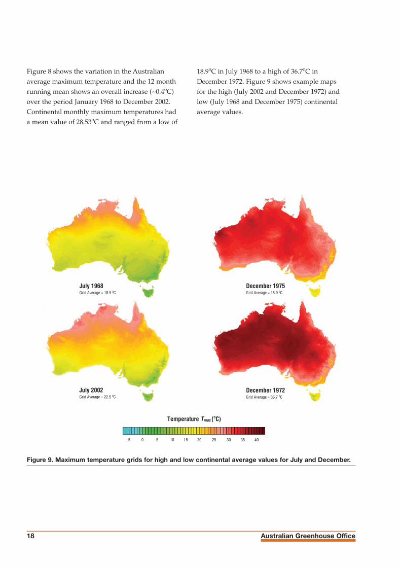
Figure 8 shows the variation in the Australianaverage maximum temperature and the 12 monthrunning mean shows an overall increase (~0.4oC)over the period January 1968 to December 2002.Continental monthly maximum temperatures hada mean value of 28.53oC and ranged from a low of
18.9oC in July 1968 to a high of 36.7oC inDecember 1972. Figure 9 shows example mapsfor the high (July 2002 and December 1972) andlow (July 1968 and December 1975) continentalaverage values.
Figure 9. Maximum temperature grids for high and low continental average values for July and December.
July 1968Grid Average = 18.9 0C
July 2002Grid Average = 22.5 0C
December 1972Grid Average = 36.7 0C
December 1975 Grid Average = 18.9 0C
5 10 15 20-5 0 30 35 4025
Temperature Tmax (oC)
National Carbon Accounting System Technical Report 19
2.2.5.3 Minimum Temperature
Monthly maximum temperature (Tmin) was fittedfrom data from the BoM monthly minimumtemperature data set. Any month which had lessthan 15 days recorded measurements was removedfrom the data set and all years which did not have12 months of data were also removed. The averagenumber of station numbers used for all years was516, ranging from 363 stations in 1986 to 733stations in 2002.
Both spline and partial spline functions were fittedto the BoM data. A second order spline functionusing three independent variables (longitude,latitude and elevation) was used to create theminimum temperature surfaces. The average errorassociated with the maps ranged from 0.6 to 1.0oC.
Figure 10 shows the variation in the Australianaverage minimum temperature and the 12 monthrunning mean shows an overall increase (~0.5oC)over the period January 1968 to December 2002.Figure 11 shows the continental monthly minimumtemperatures have a mean value of 14.8oC andranged from a low of 5.5oC in July 1982 to a high of22.3oC in February 1983. Figure 11 shows examplemaps for the high (February 1983 and July 1973)and low (February 1972 and July 1982) continentalaverage values.
Figure 10. Australian average minimum temperature (Tmin) and the 12 month running mean.
1968
1969
1970
1971
1972
1973
1974
1975
1976
1977
1978
1979
1980
1981
1982
1983
1984
1985
1986
1987
1988
1989
1990
1991
1992
1993
1994
1995
1996
1997
1998
1999
2000
2001
2002
Year
Degr
ees
o C
Minimum Temperature
0.00
5.00
10.00
15.00
20.00
25.00
Tmin12 per. Mov. Avg. (Tmin)

Australian Greenhouse Office20
2.2.5.4 Rainfall
Rainfall (P) was fitted to the data from the BoMmonthly rainfall data set. Any month in which hadless than 20 days recorded measurements wasremoved from the data set and all years which didnot have 12 months of data were also removed fromthe data set. The average number of station numbersused for all years was 5,972 ranging from 4,719stations in 1994 to 7,080 stations in 1970.
A second order spline function using threeindependent variables (longitude, latitude andelevation) and a square root transformation wasused to create the rainfall surfaces. The average
grid values ranged from 15.5 mm in November1982 to 219 mm in January 1974. The errorassociated with the grids ranged from 14% to 30%,with the higher errors resulting from the lower thanaverage value grids.
Figure 12 shows the Australian continental averagemonthly and annual rainfall. The mean value forthe continental monthly average is 40 mm andranges from a low of 7 mm in October 2002 to ahigh of 235 mm in January 1974. The mean annualrainfall was 485 mm and ranged from 327 mm in2002 to 770 mm in 1974. Figure 13 shows annualrainfall maps for 1970 to 2002.
July 1982Grid Average = 5.5 0C
July 1973Grid Average = 10.0 0C
February 1983Grid Average = 22.3 0C
February 1972 Grid Average = 20.10C
5 10 15 20-5 0 30 35 4025
Temperature, Tmin (oC)
Figure 11. Minimum temperature grids for high and low continental average values for July and February.
National Carbon Accounting System Technical Report 21
Figure 12. Australian continental average monthly rainfall.
0
50
100
150
200
250
1968
1969
1970
1971
1972
1973
1974
1975
1976
1977
1978
1979
1980
1981
1982
1983
1984
1985
1986
1987
1988
1989
1990
1991
1992
1993
1994
1995
1996
1997
1998
1999
2000
2001
2002
Monthly Rainfall
0
100
200
300
400
500
600
700
800
900
1968
1969
1970
1971
1972
1973
1974
1975
1976
1977
1978
1979
1980
1981
1982
1983
1984
1985
1986
1987
1988
1989
1990
1991
1992
1993
1994
1995
1996
1997
1998
1999
2000
2001
2002
Annual Rainfall
Year
Year
(mm
)(m
m)

Australian Greenhouse Office22
Figure 13. Annual rainfall 1970–2002.
1970 1971 1972 1973 1974
1975 1976 1977 1978 1979
1980 1981 1982 1983 1984
1985 1986 1987 1988 1989
1990 1991 1992 1993 1994
1995 1996 1997 1998 1999
2000 2001 2002
Rainfall, P (mm)
0 100 200 300 400 500 1000 2000

National Carbon Accounting System Technical Report 23
2.2.5.5 Frost Days
The number of frost days per month (F) was fitted tothe data from the BoM monthly data set. Any monthwhich had less than 20 days recorded measurementswas removed from the data set and all years whichdid not have 12 months of data were also removed.The average number of station numbers used for allyears was 548, ranging from 350 stations in 2002 to739 stations in 1973.
A second order spline function using threeindependent variables (longitude, latitude andelevation) was used to create the frost surfaces.Values on the output grids which were greater thanthe number of days in the month were reduced tothe number of days in the month and any valuesless than 0 were converted to 0. The continentalaverage annual number of frost days ranged from21.1 days in 1982 to 6.1 days in 1991(Figures 14and 15) with a sharp decline in the latter half ofthe period. The error associated with the datagrids ranged from 0.01 days in the summermonths to 3 days in the winter months, with thehigher errors resulting from the higher thanaverage value grids.
Figure 14. Australian continental average annual number of frost days.
Annual number of frost days
0
5
10
15
20
25
1968
1969
1970
1971
1972
1973
1974
1975
1976
1977
1978
1979
1980
1981
1982
1983
1984
1985
1986
1987
1988
1989
1990
1991
1992
1993
1994
1995
1996
1997
1998
1999
2000
2001
2002
Days
Year
Australian Greenhouse Office24
2.2.5.6 Radiation
As the BoM monthly data would not support thederivation of monthly surfaces, long-term averageswere used. For monthly productivity it was decidedthat ‘flat earth’ estimates of global radiation wouldbe used as slope and aspect correction at the 1 kmscale was thought to be inappropriate. The radiationwith rainfall surfaces from ANUCLIM were used.Grids of net radiation were derived where:
RN = (RP * 0.8) - 4) if RP > 5
RN = 0 if RP <= 5 (7)
2.3 NORMALISED DIFFERENCEVEGETATION INDEX (NDVI)
The NDVI provides a crude estimate of vegetationhealth and a means of monitoring changes invegetation over time and is one of the most commonvegetation indices derived from remotely senseddata. NDVI is related to vegetation as healthyvegetation reflects very well in the near infrared partof the spectrum. Green leaves have a reflectance of20 percent or less in the 0.5 to 0.7 micron range(green to red, λR) and about 60 percent in the 0.7 to1.3 micron range (near infra-red, λI). The value isthen normalised to the range –1 <= NDVI <= 1 to
partially account for differences in illumination andsurface slope but is undefined when λR and λI arezero. The NDVI is computed by the product of theratio of the two electromagnetic wavelengths.
NDVI = (λI -λR)/( λI +λR) (8)
The typical range is between about -0.1 (λI less thanλR for a not very green area) to 0.6 (for a very greenarea). NDVI values vary with absorption of red lightby plant chlorophyll and the reflection of infraredradiation by water-filled leaf cells. Becausephotosynthesis occurs in the green parts of plantmaterial the NDVI is normally used to estimategreen vegetation.
The Advanced Very High Resolution Radiometer(AVHRR) sensor collects imagery at a 1 kmresolution that is then used to generate a NDVIproduct for Australia. The Environmental ResourcesInformation Network (ERIN) of the AustralianGovernment Department of Environment andHeritage .01 degree NDVI archive contains datafrom the National Oceanic and AtmosphericAdministration (NOAA) Satellite 9, 11, 14 and 16.The NOAA 14 data is calibrated using the equationsin ‘Revised post-launch calibration of channels 1 and2 of the AVHRR on board the NOAA-14 spacecraft’by Rao and Chen on the NOAA web site at
Figure 15. Example grids of low (1991, average = 6.1 days), medium (1987, average =14.0 days) and high(1982, average = 21.1 days) number of days frost.
1991 1987 1982
Annual Frost days, F
0 10 30 455 2015 3525 5040
National Carbon Accounting System Technical Report 25
http://orbit-net.nesdis.noaa.gov/. Data fromNOAAs 9, 11 and 16 are cross-calculated to NOAA14 by assuming that the reflectance of the 10,000pixels with the lowest standard deviation in theNOAA 14 dataset from each of 5 of AustralianDeserts are stable.
The data for April to September 1994 obtained fromNOAA 11 was very poor due to very low sunangles, thus large angular corrections. For thisperiod, NOAA 9 NDVI images were calibrated andthen composited into the NOAA 11 image data.
The images were cloud screened by masking outpixels that did not appear to be biologicallyconsistent with the pixels in the images takenimmediately before and after. The first stage of thisprocess was performed by a filter that masks outpixels that show a large decrease followed by a largeincrease. This procedure was also designed toremove ‘dropout’ values and abnormally highvalues probably associated with low sun angles.This was followed by a manual (subjective) stagewhere suspect areas were compared on screen withadjacent images. The cloud masks were thenadjusted as required. It should be noted that thescreening procedure contained a degree ofsubjectivity and was not exhaustive and the cloudmasks were expected to change slightly with furtherwork (N. Fitzgerald pers. comm.).
NDVI values were available for the ten year period,1991 to 2000. Long-term averages were derived fromthe data and used in both the long-term andmonthly productivity indices to provide acomprehensive cloud free data set. Monthly andannual data were not usable because of the extent ofcloud cover obscuring data signals over the shortertime spans.
The 28 day average NDVI (in BIL file format)(NDVIb) files supplied by ERIN had values whichranged from 1 to 256. NDVI values less than 50 wereconsidered to be cloud and given a no data value of-99. For each month NDVI was then rescaled:
NDVI = (NDVIb - 50)/200 if NDVIb > 50
NDVI = -99 if NDVIb <= 50 (9)
The satellite-derived NDVI data represents thephotosynthetic capacity of all vegetation within a 1km pixel for a given month, correlated with thefraction of photosynthetically active radiation (PAR)absorbed (fPAR). Sellers (1985, 1987) derived animportant relationship between leaf area index(LAI), absorbed photosynthetically active radiation(APAR) and NDVI. This research found that underspecified canopy properties APAR was linearlyrelated to NDVI and curvilinear related to LAI. LAIis usually positively corelated to an increase inthe difference between λI and λR radiation. Thisrelationship has been shown to hold generallyover a number of different biomes. LAI can becalculated from:
LAI = ln ( 1 - (NDVI * 1.0611) + 0.3431) / - 0.5 (10)

year and Topt as equal to the average of Tlow andThigh. Tavg was the average temperature described inSections 2.2.4.1 and 2.2.5.1. The equation describingthe effects of temperature is:
(11)
Tlow represents the monthly average temperaturebelow which plant growth stops; Thigh is the monthlyaverage temperature above which plant growthstops and Topt is the optimum temperature forgrowth. Minimum and maximum temperature datawere derived from the ESOCLIM and ANUSPLINpackages and Tavg Thigh, Tlow and Topt were derivedfrom these values. The temperature modifier (Tmod)was 1 when Tavg = Topt. Equation 10 gives ahyperbolic response curve, with Tmod = 0 when Tavg = Tlow or Thigh. Consequently Tmod generally hadrelatively small effects on the calculation of plantproductivity. Figure 16 shows the spatialtemperature modifier equations for Januaryand July long-term averages.
Australian Greenhouse Office26
Tmod =Tavg - Tlow
Topt - Tlow
Thigh - Tavg
Thigh - Topt
Figure 16. Temperature modifier spatial equations (from Equation 11) for January and July long-term averages.
January
Tmod
Tavg Tlow
Topt Tlow
Thigh Tavg
Thigh Topt
=
July
Tmod
= Tavg Tlow
Topt Tlow
Thigh Tavg
Thigh Topt
Temperature modifier, Tmod Temperature (oC)
100 20 300 0.5 1
3. CALCULATION OF PLANT PRODUCTIVITY
Monthly values of environmental constraints onproductivity indices were expressed by modifierscalculated from the temperature, vapour pressuredeficit (VPD) of the atmosphere, soil water deficitand number of frost days.
3.1 TEMPERATURE MODIFIERThe growth of any plant species is limited bytemperatures outside the optimum range for thatspecies. A general assumption is made that, in anyparticular region, the plants are well-adapted to theexisting temperature range. Tlow was set to 1⁄2 theminimum temperature of the coldest month if theminimum temperature of the coldest month wasgreater than or equal to 0. If the minimumtemperature of the coldest month was less than 0,Tlow was set to 1⁄2 the minimum temperature of thecoldest month plus the minimum temperature of thecoldest month. Thigh was set to 5oC above themaximum temperature of the hottest month of the
( )

Number of Frost days per month, F
= 1 –
Frost modifier, Fmod
0 2 10 306
: 31
0 0.5 1 15
July
National Carbon Accounting System Technical Report 27
3.2 FROST MODIFIERA frost modifier (Fmod) was applied, using the simpleassumption that frost temporarily inactivates thephotosynthetic mechanism in foliage, so there isno growth on a frost day. The modifier is simplyone minus of number of frost days per month (F)divided by the number of days in the month(Figure 17).
Fmod = (1 - F / Days in month) (12)
3.3 VAPOUR PRESSURE DEFICIT (VPD)MODIFIER
The VPD modifier is important because plantsrespond to the VPD rather than relative humidityand the VPD provides the driving force forevaporation of water from the leaves. There is agradient of water vapour from the leaves to the airbecause the air in the leaf is saturated whereas theair outside is drier. The larger the VPD the steeperthe gradient. The VPD acting on stomatal, andhence canopy, conductance. The equation used is:
VPDmod = Exp(-0.05 * VPD) (13)
Figure 18 shows the VPD modifier spatial equationsfor the January and July long-term averages. Thismodifier essentially acts as a control on the rate ofwater loss; it is conditional upon soil water balance(see over page).
Figure 17. The frost modifier equation for the July long-term average.

Australian Greenhouse Office28
3.4 SOIL WATER CONTENT (SW)Soil water content (SW) is derived from waterbalance calculations, which take into account themaximum soil water holding capacity (SC) in theroot zone of plants. Plant water use, transpiration(Trans), is calculated from the equation forequilibrium evaporation (Eeq, see Landsberg andGower 1997; p 79), modified by feed-back fromcurrent soil water content, and a conventionalwater balance equation:
Eeq = ((0.67 * RN * (1 - 0.05)) / 2.47) * days in month (14)
Where Eeq is the equilibrium evaporation and RN isthe net radiation (see Equation 7)
Monthly transpiration (Trans) was calculated as:
Trans(j) = Eeq(j) * SWmod(j-1) (15)
Where Trans(j) is the transpiration for the month (j),Eeq(j) is the equilibrium evaporation for the monthand SWmod(j-1) is the soil water modifier (seeEquation 20) for the previous month (Figure 20).
Rainfall interception (I) is derived from the leaf areaindex (LAI) and is defined as:
I = 0.05 + (0.02 * LAI) (16)
Australian continental rainfall interception (I)values were derived for long-term averages onlyas monthly data was not available for the period1970 to 2002. Figure 21 shows the long-term averageI for January.
Figure 18. VPD modifier spatial equations for January and July long-term averages.
0 2010 30
= exp – 0.05 *
January
0 0.5 1
= exp – 0.05 *
VPD
July
VPDmod
VPDmod VPD
Vapour Pressure Deficit,VPDVPDmod
National Carbon Accounting System Technical Report 29
January 1995
= * (1 – 0.05)
* 312.47
0
Equilibrium evaporation, Eeq (mm)
100 200 0
Net radiation, RN (MJm-2day-1)
10 20 30 40
0.67 *
0
Equilibrium evaporation, Eeq (mm)
100 200
= *
Transpiration (mm)
0 200
Soil water modifier, SWmod (mm)
0.5 10
December 1994January 1995
Figure 19. Spatial equation for equilibrium evaporation, January 1995.
Figure 20. Spatial equation for transpiration, January 1995.
January
0
Intercept
0.5 0
Leaf Area Index, LAI
5 10
= 0.05 + 0.02 *
Figure 21. Spatial equation for interception, January long term average.
Australian Greenhouse Office30
January 1995
=
0
Soil water, SW (mm)
100 200 300 400 500 0
Soil water, SW (mm)
100 200 300 400 500
+
Water balance (mm)
-200 6000 200 400 800
December 1994 January 1995
Figure 23. Spatial equation for soil water content, January 1995.
The conventional water balance (W) equation isderived from the rainfall (P), the rainfall interception(I) and transpiration (Trans) and is given by:
W = (P * (1 - I)) – Trans (17)
Figure 22. Spatial equation for water balance, January 1995.
January 1995
0
Rainfall, P (mm)
1000
Transpiration (mm)
* 1 –= –
0 0.5
InterceptWater balance, W (mm)
0 200200 400 800 1700-200 6000 200 400 800
The soil water content (SW) is derived by adding thewater balance (change in soil water content over themonth) (W) to the previous months soil watercontent (Equation 18, Figure 23). The soil watercontent is reduced to the soil water holding capacityif it is greater than soil holding water capacity.Negative soil water content values are set to zero.
SW(j) = SW(j-1) + W (18)

National Carbon Accounting System Technical Report 31
Initial (first month) SW was taken as 0.75 of the soilwater holding capacity (SC) and carries over fromone time step to the next. The soil moisturecalculation was sequenced so that initial SW was setby running the water balance model for two yearsprior to initiating the productivity model. For theJanuary 1970 to December 2002 monthly analysis,the SW calculation sequence was initialised using the1968 and 1969 climate data.
The soil water modifier (SWmod) (Equation 20) wascalculated from the moisture ratio (M), which is theSW divided by SC. The equation describes thevariable effect of M across the range from wet soil(M ≈ 1) to dry soil (M ≈ 0).
M = SW / SC (19)
0
Moisture ratio, M
0.5 1
=
Soil water, SW (mm)
0 250 500
Soil water holding capacity, SC (mm)
0 100 200 300
January 1995
Figure 24. Spatial equation for moisture ratio, January 1995.
The soil water and VPD modifiers are notmultiplicative; the lowest one applies. The argumentis that if plant growth (conversion of radiant energyinto biomass) is limited more by VPD than soilwater (i.e. if VPDmod < SWmod) then soil water is not alimiting factor, even if soil water content is relativelylow. The converse applies; i.e. if SWmod < VPDmod, soilwater is the limiting factor.
SWmod = 1 / (1 + ((1 - M) / 0.6)7 ) if 1 /(1 + ((1 - M) / 0.6)7 ) < VPDmod
SWmod = VPDmod if 1 / (1 + ((1 - M) / 0.6)7 ) > VPDmod (20)
Australian Greenhouse Office32
not used to infer an absolute mass increase. Usedin this way the conversion factor was not critical asit had only a linear (direct multiplicative) effect onthe index.
Absorbed photosynthetically active radiation(APAR) was estimated from global solar radiation,interpolated from station data provided by the BoM,and from a linear relation with the satellite-derivedNDVI which represents the photosynthetic capacityof all vegetation within each 1 km pixel and iscorrelated with the fraction of PAR absorbed (fPAR).
APAR is calculated as half the amount of short-wave(global) incoming radiation (RP) absorbed by plantcanopies:
APAR = RP * 0.5 * (1 - Exp(-0.5 * LAI)) x days in month (21)
= lesser of 1 + 1 -
January 1995
0
Soil water modifier, SWmod
0.5 1 0
Moisture ratio,M
0.5 1
0
Vapour Pressure Deficit modifier, VPDmod
0.5 1
0.6
1
7
or
Figure 25. Spatial equation for soil water modifier, January 1995.
3.5 ABSORBED PHOTOSYNTHETICALLYACTIVE RADIATION (APAR)
In the original version of the 3-PG model (followingLandsberg and Waring 1997), APAR is multipliedby a factor that converts it to a biomassaccumulation equivalent. This, in effect,amalgamates two physiological processes: theconversion of absorbed CO2 into initial carbonproducts (gross primary production) and the loss ofa proportion of those products by respiration to givenet primary productivity. The value of theconversion factor (ε, gm C MJ-1 APAR) used wasobtained from the literature (Potter et. al. 1993,Ruimey et. al. 1994, Landsberg et. al. 1997). There issignificant variation in ε values, but no clear patternin relation to plant type, so a ‘best estimate’ value of1.25 gm C MJ-1 APAR was used. In the productivitymodel the net primary productivity equivalent wastaken as an index of ‘plant productivity’ and was

National Carbon Accounting System Technical Report 33
Where LAI is the Leaf Area Index and the coefficient0.5 is a general value for the extinction coefficient.In a slope and aspect corrected form of theproductivity model radiation with rainfall (RP) isreplaced by slope and aspect corrected radiation(RC). APAR was calculated for long-term meansas the available radiation and LAI data were long-term averages.
3.6 PLANT PRODUCTIVITY INDEXProductivity is reduced by modifiers reflecting non-optimal nutrition, soil water status, temperatureand atmospheric vapour pressure deficits. Modifiersare dimensionless factors with values between0 (complete restriction of growth) and1 (no limitation). Modifiers used in this way arediscussed by Landsberg (1986), McMurtrie et. al.
(1994) and Landsberg and Waring (1997).
0 5 10
1 – exp – 0.5 *
January
0 250 500
July
Leaf Area Index, LAIAbsorbed Photosynthetically
Active Radiation, APAR
= * 31* 0.5 *
Radiation (MJ m-2 day-1)
400 10 20 30
* 31* 0.5 *= 1 – exp – 0.5 *
Figure 26. Long-term average APAR for January and July.
January
=
July
Plant Productivity Index
* 0.01* * * *
Temperature modifier, Tmod Soil water modifer, SWmodSoil nutrient status, SN Frost modifier, Fmod
0 250 5000 1 5 0 0.5 1 0.75 1.0 1.25 0 0.5 1 0 0.5 1
= * 0.01* * * *
Absorbed Photosynthetically Active Radiation, APAR
Figure 27. Spatial equations for productivity indices, January and July long-term averages.

Australian Greenhouse Office34
Plant Productivity Index
0 1 2 3 5 10 15 25
Monthly values of plant productivity index(Figure 27) are expressed by APAR multiplied bythe modifiers calculated from soil waterbalance, temperature, number of frost days andsoil nutrient values.
Productivity Index = APAR * Tmod * SN *SWmod * 0.01 * Fmod (22)
Figure 28. Derived long-term average plant productivity index for Australia.
Productivity Indexann=Σj=12
j=1Productivity Indexj
Australia’s annual plant productivity is the sum ofthe 12 monthly values for the year of interest
(23)
where j is the month. Figure 28 shows the long-termannual average productivity index for Australia andFigure 29 shows the annual productivity indices for1970 to 2002.
A comparison of the annual productivity indexmaps in Figure 29 and the annual rainfall maps(Figure 13) shows the dominance of rainfall in theestimation of plant productivity.

National Carbon Accounting System Technical Report 35
1970 1971 1972 1973 1974
1975 1976 1977 1978 1979
1980 1981 1982 1983 1984
1985 1986 1987 1988 1989
1995 1996 1997 1998 1999
Plant Productivity Index
2000 2001 2002
1990 1991 1993 19941992
0 1 2 3 5 10 15 25
Figure 29. Derived annual continental productivity indices 1970-2002.

4. SELECT REFERENCES
AUSLIG 1994. GEODATA TOPO–250K Data User
Guide, Version 1 Data, Edition 2. AustralianSurveying & Land Information Group,Commonwealth Department of AdministrativeServices, Canberra, Australia.
Bates, D. & Wahba, G. 1982. Computational methods
for generalised cross-validation with large data sets. InBaker, C. and Miller, G. (eds), Treatment ofIntegral Equations by Numerical Methods,Academic Press, London.
Eldén L. 1984. A note on the computation of the
generalized cross-validation function for ill-
conditioned least squares problems. BIT 24:467-472.
Hillel, D. 1980. Applications of Soil Physics.
Academic Press, New York.
Hutchinson, M.F. 2001. ANUSPLIN User Guide
Version 4.2. Centre for Resource andEnvironmental Studies, Australian NationalUniversity, Canberra.
Hutchinson, M.F. 2000. ANUDEM Software. Centrefor Resource and Environmental Studies,Australian National University, Canberra.http://cres.anu.edu.au/outputs/ software.html
Hutchinson, M.F. 1998a. Interpolation of rainfall data
with thin plate smoothing splines: I. Two dimensional
smoothing of data with short range correlation.
Journal of Geographic Information and DecisionAnalysis 2(2):153-167. http://www.geodec.org/gida_4.htm
Hutchinson, M.F. 1998b. Interpolation of rainfall data
with thin plate smoothing splines: II. Analysis of
topographic dependence. Journal of GeographicInformation and Decision Analysis 2(2):168-185.http://www.geodec.org/gida_4.htm
Hutchinson, M.F. 1995. Interpolating mean rainfall
using thin plate smoothing splines. InternationalJournal of GIS 9:385-403.
Hutchinson, M.F. 1993. On thin plate splines and
kriging. In Tarter, M.E. & Lock, M.D. (eds),Computing Science and Statistics, Vol. 25.Interface Foundation of North America,University of California, Berkeley, pp. 55-62.
Hutchinson, M.F. 1991a. The application of thin plate
smoothing splines to continent-wide data assimilation.
In Jasper, J.D. (ed), BMRC Research Report No.27,Data Assimilation Systems, Bureau ofMeteorology, Melbourne, pp. 104-113.
Hutchinson, M.F. 1991b. Climatic analyses in data
sparse regions. In Muchow, R.C. & Bellamy, J.A.(eds), Climatic Risk in Crop Production, CABInternational, Wallingford, pp. 55-71.
Hutchinson, M.F. 1989. A new objective method for
spatial interpolation of meteorological variables from
irregular networks applied to the estimation of
monthly mean solar radiation, temperature,
precipitation and windrun. CSIRO Division of WaterResources Research Technical Memorandum89/5: 95-104.
Hutchinson, M.F. 1984. A summary of some surface
fitting and contouring programs for noisy data.
CSIRO Division of Land Use Research andMathematics and Statistics, Consulting ReportNo. ACT 84/6, CSIRO, Canberra.
Hutchinson, M.F. & Bischof, R.J. 1983. A new method
for estimating the spatial distribution of mean seasonal
and annual rainfall applied to the Hunter Valley,
New South Wales. Australian MeteorologicalMagazine 31: 179-184.
Hutchinson, M.F., Booth, T.H., McMahon, J.P. & Nix,H.A. 1984. Estimating monthly mean values of daily
total solar radiation for Australia. Solar Energy 32:277-290.
Hutchinson, M.F. & Gessler, P.E. 1994. Splines - more
than just a smooth interpolator. Geoderma 62: 45-67.
Australian Greenhouse Office36

National Carbon Accounting System Technical Report 37
Hutchinson, M.F., Houlder, D.J., Nix, H.A. &McMahon, J.P. 1999. ANUCLIM User Guide,
Version 5.0. Centre for Resource andEnvironmental Studies, Australian NationalUniversity, Canberra.
Hutchinson, M.F., Nix, H.A. & McMahon, J.P. 1992.Climate constraints on cropping systems. In Pearson,C.J. (ed), Field Crop Ecosystems of the World,Elsevier, pp 37-58.
Hutchinson, M.F., Nix, H.A., McMahon, J.P. & Ord,K.D. 1996. The development of a topographic and
climate database for Africa. In Proceedings of theThird International Conference/Workshop onIntegrating GIS and Environmental Modelling,NCGIA, Santa Barbara, California. Also onNCGIA Web Page.http://www.ncgia.ucsb.edu/conf/SANTA_FE_CD-ROM/main.html
Hutchinson, M.F., Stein, J.L. & Stein, J.A. 2000.Derivation of nested catchments and sub-catchments
for the Australian continent. Centre for Resourceand Environmental Studies, Australian NationalUniversity, Canberra.http://cres.anu.edu.au/outputs/ programs.html
Hutchinson, M.F., Stein, J.A. & Stein, J.L. 2001.Upgrade of the 9 Second Digital Elevation Model for
Australia. Centre for Resource and EnvironmentalStudies, Australian National University, Canberra.http://cres.anu.edu.au/outputs/programs.html
Kesteven, J.L. 1998. A Spatial and Temporal Analysisof Australian Climate Fields, PhD Thesis, ANU,November 1998.
Kesteven, J.L. & Hutchinson, M.F. 1996. Spatial
modelling of climatic variables on a continental scale.
In Proceedings of the Third InternationalConference/Workshop on Integrating GIS andEnvironmental Modelling, NCGIA, Santa Barbara,California. Also on NCGIA Web Page.http://www.ncgia.ucsb.edu/conf/SANTA_FE_CD-ROM/main.html
Landsberg, J. J. 1986. Physiological Ecology of Forest
Production. Academic Press, Sydney, 198 pp.
Landsberg, J.J., & Gower, S.T. 1997. Application of
Physiological Ecology to Forest Management.
Academic Press, San Diego, California. 354p.
Landsberg, J.J. & Waring, R.H. 1997. A generalised
model of forest productivity using simplified concepts
of radiation-use efficiency, carbon balance and
partitioning. Forest Ecology and Management95:209–228.
Landsberg, J.J., Prince, S.D., Jarvis, P.G., McMurtrie,R.E., Luxmoore, R. & Medlyn, B.E. 1997. Energy
conversion and use in forests: An analysis of forest
production in terms of radiation utilisation efficiency.
In The Use of Remote Sensing in the Modeling ofForest Productivity at Scales from the Stand to theGlobe. (eds) Gholz, H.L., Nakane, K., andShimoda, H. Kluwer Academic Publishers:Dordrecht.
Laslett, G.M. 1994. Kriging and splines: An empirical
comparison of their predictive performance in some
applications. Journal of the American StatisticalAssociation 89:391-409.
Laslett, G.M., McBratney, A.B., Pahl, P.J. &Hutchinson, M.F. 1987. Comparison of several spatial
prediction methods for soil pH. Journal of SoilScience 38, 325-341.
McKenney, D.W., Hutchinson, M.F., Kesteven, J.L. &Venier, L.A. 2001 Canada’s plant hardiness zones
revisited using modern climate interpolation
techniques. Canadian Journal of Plant Sciences 81:129-143.
McKenzie, N. J. & Hook, J. 1992. Interpretations of the
Atlas of Australian Soils. Consulting Report to theEnvironmental Resources Information Network(ERIN). CSIRO Division of Soils Technical Report94/1992.

Australian Greenhouse Office38
McMurtrie, R.E., Gholz, H.L., Linder, S. & Gower,S.T. 1994. Climatic factors controlling the productivity of
pine stands: a model-based analysis. EcologicalBulletins, 43: 173-188.
McKenzie, N.J., Jacquier, D.W., Ashton, L.J. &Cresswell, H.P. 2000. Estimation of Soil Properties
Using the Atlas of Australian Soils, CSIRO Landand Water Technical Report 11/00.
Northcote, K.H. with Beckmann, G.G., Bettenay, E.,Churchward, H.M., Van Dijk, D.C., Dimmock,G.M., Hubble, G.D., Isbell, R.F., McArthur, W.M.,Murtha, G.G., Nicolls, K.D., Paton, T.R.,Thompson, C.H., Webb, A.A. & Wright, M.J. 1960-1968. Atlas of Australian Soils, Sheets 1 to 10.With explanatory data (CSIRO Aust. andMelbourne University Press: Melbourne).
Northcote, K.H., Hubble, G.D., Isbell, R.F.,Thompson, C. H. & Bettenay, E. 1975.A Description of Australian Soils. (CSIRO:Melbourne).
Potter, C.S., Randerson, J.T., Field, C.B., Matson,P.A., Vitousek, P.M., Mooney, H.A. & Klooster,S.A. 1993. Terrestrial ecosystem production: A process
model based on global satellite and surface data.
Global Biogeochemical Cycles 7:811–841.
Price, D.T., McKenney, D.W., Nalder, I.A.,Hutchinson,M.F. & Kesteven, J.L. 2000. Acomparison of two statistical methods for spatial
interpolation of Canadian monthly mean climate data.
Agricultural and Forest Meteorology 101: 81-94.
Ruimey, A., Saugier, B. & Dedieu, G. 1994.Methodology for the estimation of terrestrial net
primary production from remotely sensed data. J.Geophys. Res. 99:5263–5283.
Sellers, P.J. 1985. Canopy Reflectance, Photosynthesis
and Transpiration. International Journal of RemoteSensing, 68:1335-1372.
Sellers, P.J. 1987. Canopy Reflectance, Photosynthesis,
and Transpiration 2. The role of Biophysics in the
Linearity of Their Interdependence. Remote Sensingof the Environment, 21:143-183.
Stace, H.C.T., Hubble, G.D., Brewer, R., Northcote,K.H., Sleeman, J.R., Mulcahy, M.J. & Hallsworth,E.G. 1968. A Handbook of Australian Soils. RellimTech. Publ.: Glenside, S. A.
Wahba G. 1979. How to smooth curves and surfaces
with splines and cross-validation. Tech. Report 555.University of Wisconsin-Madison, StatisticsDepartment.
Wahba G. 1990. Spline Models for Observational Data.
CBMS-NSF Regional Conference Series inMathematics 59. SIAM, Philadelphia. Society forIndustrial and Applied Mathematics, 169pp.

National Carbon Accounting System Technical Report 39
APPENDIX 1
Preliminary Investigations: Spatial Estimation of Plant Productivity and Classification of Non-Commercial Vegetation Types
URS Australia
Joe Landsberg
Jenny Kesteven
July 2001

Australian Greenhouse Office40
National Carbon Accounting System Technical Report 41
TABLE OF CONTENTSPage No.
A1. Overview 43
A2. Collation and Analysis of Growth Data – URS Australia 44
A2.1 Assembly of Datasets 44
A2.2 Coding 45
A2.3 Selection of Vegetation Types 45
A2.4 Preparation of Growth Tables 45
A2.5 Findings 45
A2.5.1 Review of Publications 45
A2.5.2 Comparability Issues and Adjustment Factors 47
A2.5.3 Forest Growth Data 47
A2.6 Discussion 48
A2.7 References 48
A3. Spatial Estimation of Plant Productivity – Joe Landsberg & Jenny Kesteven 50
A3.1 Introduction 50
A3.2 Background 50
A3.3 Planning and Procedure 50
A3.4 The Plant Productivity Model 52
A3.5 Analysis of Plant Productivity by IBRA Regions 52
A3.6 Plant Productivity Values by IBRA Regions 53
A3.7 Spatial Variation in Plant Productivity within Regions 55
A3.8 Analysis of Plant Productivity by Carnahan Vegetation Classes 62
A3.9 Conclusions 63
A3.10 Follow Up Research 64
A3.11 Relevant Citations 64
A4. Forest Growth Data Tables – URS Australia 65
LIST OF TABLESPage No.
Table 1a. Growth data for sites in South Australia, Hassall & Associates (1999a). 66
Table 1b. Growth data for sites in Victoria, Hassall & Associates (1998). 74
Table 1c. Growth data for sites in Western Australia, Hassall & Associates (1999b). 81
Table 2a. Growth data for sites in South Australia, Wong et. al. (2000). 88
Table 2b. Growth data for sites in Victoria, Wong et. al. (2000). 92

Australian Greenhouse Office42
LIST OF FIGURESPage No.
Figure 1. Derived long-term average plant productivity index for Australia. 52
Figure 2. Annual average Plant Productivity by IBRA regions. 53
Figure 3. Monthly plant productivity index in four IBRA regions: South East Highlands (SEH); Jarrah Forest (JF); Darling River Plains (DRP); and Central Kimberly (CK). 54
Figure 4. Monthly water balance in the four IBRA regions for which plant productivity data are shown in Figure 3. Negative values indicate the dryness of the area but note that in thecalculation of water balances for the model soil water content cannot go below zero. 55
Figure 5a. Change in the standard error of the mean productivity value with various numbersof sample points, up to 100, in the Wet Topics region. There was no indication that a minimum value had been reached. b. Spatial distribution of plant productivity across the Wet Tropics region. The data exhibit significant variation. 56
Figure 6a. Change in the standard error of the mean productivity value with various numbersof sample points, up to 100, in the Tanami Desert region. There was no indication thata minimum value had been reached. b. Spatial distribution of mean annual plantproductivity across the Tanami Desert. The data exhibit significant variation, with a marked peak in the low productivity range. 57
Figure 7a. Change in the standard error of the mean productivity value with various numbers of sample points, up to 300, in the Jarrah Forest region. The curve indicates that 2-300 samplepoints would be required to give an accurate value of the mean. b. Spatial distributionof mean annual plant productivity across the Jarrah Forest region. The curve is skewedtowards lower values. 58
Figure 8a. Change in the standard error of the mean productivity value with various numbers of sample points, up to 300, in the South Eastern Highlands. The curve indicates that 2-300 sample points would be required to give an accurate value of the mean. b. Spatial distribution of mean annual plant productivity across the South Eastern Highlands region. The distribution is more uniform than in most other regions. 59
Figure 9a. Change in the standard error of the mean productivity value with various numbersof sample points, up to 300, in the Darling River Plains. The curve indicates that at least 300 sample points would be required to give an accurate value of the mean. b. Spatial distribution of mean annual plant productivity across the Darling River Plains. The distribution is reasonably uniform, slightly skewed to the higher values. 60
Figure 10a. Change in the standard error of the mean productivity value with varying numbers ofsample points, up to 300, in the Central Kimberley region. The curve has not reached stablevalues; at least 300 sample points would be required to give an accurate value of the mean. b. Spatial distribution of mean annual plant productivity across the Central Kimberleyregion. The distribution is approximately normal. 61
Figure 11. The distribution of open woodland shaded by the plant productivityindex value. 62
Figure 12. Range of plant productivity values for the forest classes of present Carnahanvegetation classes. 63

National Carbon Accounting System Technical Report 43
A1. OVERVIEW
The work reported here represents preliminaryinvestigations toward developing the capability ofthe National Carbon Accounting System (NCAS) toestimate carbon sequestration in ‘non-commercial’vegetation types, largely environmental plantingsand native regrowth. This preliminary workprovided guidance on the preferred framework andevolution of methods presented in the main body ofthis report.
Most of the collection of forest growth data andmodelling activity has historically been focussed oncommercial plantings which have higherproductivity. Non-commercial plantings areimportant because of their associated benefits e.g.windbreaks, salinity control, erosion control, habitatand biodiversity, visual amenity. With the drive tomore sustainable land management, there is a needfor more of such plantings integrated with wholefarm and whole region planning. Likewise, nativeregrowth following disturbance, e.g. fire and landclearing, is a common feature of the Australianlandscape, and is a desirable form of revegetation.Carbon sequestration can likewise facilitate soundland management.
A relatively small, yet important, part of Australia’sNational Greenhouse Gas Inventory is the carbonstored in environmental plantings and nativeregrowth; however there are few data available onwhich to develop Growth Tables, whereby empiricalestimates may be made for specific projects or forregions. The NCAS is working to fill this gap, andthis project is a means to that end. The NCAS haschosen the second of two broad options to do so:
1. Sample stands of environmentalplantings and native regrowthsystematically across Australia, alongwith associated environmental data, anddevelop the relationships needed to developGrowth Tables; or
2. Stratify the Australian landmass on thebasis of plant productivity and use this toundertake a more-efficient stratifiedsampling and modelling of the growthpotential within these strata.
This project comprises two steps:
1. Collate and analyse available data for themain types of environmental plantings andregrowth vegetation relevant to formingGrowth Tables (as reported in SectionA2 and A4); and, concurrently
2. Develop the possible methodologies forproductivity stratification and vegetationclassification; and apply the stratificationmethodology to produce the documentedGIS layer over Australia (as reported inSection A3).
The original intent of this work was to develop aclassification method for non-commercial plantingsaround potential carbon accumulation and todevelop Growth Tables for regions of varyingproductivity throughout Australia. The aim was toclassify vegetation into a manageable number oftypes of similar carbon accumulation patterns. Thiswould provide default estimates of the carbonaccumulation for a particular vegetation class in aparticular region/location.
This was planned as a desktop study with 3 steps:
1. Draft classification of environmentalplantings and native regrowth.
a) Define classes (classification)
b) Define productivity regions (stratification);
2. Consult with experts to refine theclassification; and
3. Refine the classification.

Australian Greenhouse Office44
The initial intention was to produce a series of ‘look-up’ Growth Tables for each of the types ofnon-commercial plantings, so that they could beapplied in the relevant regions as defined in thefirst step of this project.
However, it was soon recognised that there werefew data available concerning carbon accumulationpatterns i.e. ‘plant growth rates’ of these vegetationtypes. Thus the classification would be extremelycoarse and, on its own, would add little value. Thisconclusion led to the development of methodsexplored in Richards (2002) and described indetail in Richards (2001).
In light of this, an alternative approach ofdeveloping Growth Tables for typical vegetationtypes was pursued and is reported in the followingSection A2 and data is tabulated in Section A4.
To guide data collection a list of about 40 vegetationtypes was compiled, but feedback was that thisneeded to be greatly expanded by incorporatingheight classes as well. Height class is generally usedas a site index, that is, as a measure of siteproductivity. There are few experts in this field, andthose who provided information or adviceconfirmed the paucity of this data and that it wouldbe difficult to provide the necessary Growth Tablesfor each vegetation type.
Feedback received confirmed that the best way toproceed was to collate as much of the availablegrowth information for native regrowth andenvironmental plantings that would allow potentialdevelopment of growth models and likely carbonaccumulation for particular regions. This sparse datacould then be used as a basis for interpolation,guided by relative site productivity assessments, tofill gaps. The paucity of purely ‘non-commercial’data led to the inclusion of data from somecommercial plantings data.
A2. COLLATION AND ANALYSIS OF GROWTH DATA
URS Australia
A2.1 ASSEMBLY OF DATASETSDatasets were sourced widely and because the datawere sparse, all possibilities were considered:Fortech (now URS Forestry) files, CSIRO, GreeningAustralia, State agencies, Bureau of Rural Sciences(BRS), and relevant Universities.
Data sources included:
• The Australian GovernmentBushcare/Natural Heritage Trust (NHT)funded work undertaken by Hassalls‘Measurements of Plantations of Trees in[region] to Improve the Estimates of CarbonSequestration in Low Rainfall Areas’, for thefollowing regions: South Australia, Victoriaand WA;
• The publication commissioned by the AGO(NCAS Technical Report No. 25) by Grierson,Williams and Adams (2000) which listedsources of unpublished data; and
• The ABARE Trees on Farms survey, forleads as to what might be available.(Wilson et al. 1995)
A number of other published and unpublishedreports and databases were reviewed. In mostcases, these resources did not incorporate measuredvolumetric growth data and/or were not madeavailable to URS Australia.
The surprising finding was just how little relevant
data were available, even from native forestryagencies. This was after extensive consultations.The paucity of data led to the inclusion of somecommercial plantings data. Because of this,careful consideration of the comparability andcompatibility of data was undertaken beforecalculating Growth Tables.
National Carbon Accounting System Technical Report 45
It was clear that a large volume of related dataexists, but there would be a need to establish itsutility for this particular purpose. It is likely thatfurther data will be identified and its utilityshould also be examined. Synthesis of such datahas considerable cost benefit advantages overfield sampling.
A2.2 CODINGInformation was gathered under data fields thatwould be useful for developing Growth Tables andinterpreting the variation, including:
• Site information (ID #, name/location/coordinates, year established, area planted,species list);
• Biomass estimate (value, age of trees at timeof measurement, type of estimate);
• Mean Annual Increment (MAI);
• Planting density (trees per hectare);
• Wood density (kg/m3);
• Site factors, e.g. rainfall, soil type/quality,topography, access to water, salinity;
• Husbandry, e.g. tubestock/direct seed, weedand pest control, fire, irrigation; and
• Source of information.
A2.3 SELECTION OF VEGETATION TYPESThe selection of vegetation types for analysisof growth parameters was based on twoconsiderations:
• The datasets that were made available –the best represented types can supportthe most robust Growth Tables and modelcalibrations; and
• Having a wide range of vegetation types,to give most scope for estimating theperformance of other vegetation typesby ‘interpolation’.
A2.4 PREPARATION OF GROWTH TABLESThe revised plan was that the data for each specieswould be summarised statistically to understandthe causes of variation. These have been presentedin Section A4, Tables 1 and 2.
Having compiled the growth tables and examinedthe data, it became apparent that the paucity of dataand the different methodologies used to arrive atthis data, meant that comparisons of growth and theestimation of growth tables was inappropriate.Adjustments and assumptions could be made tolessen the impacts of these incompatibilities.Undertaking these adjustments was outside thescope of this project.
A2.5 FINDINGS
A2.5.1 Review of Publications
Grierson et. al. (2000) Review of UnpublishedBiomass-Related Information: Western Australia,South Australia, New South Wales and Queensland
This presents data for mature vegetation or at leastsnap shots in time, e.g. Table 2. There are referencesto publications and datasets that may be able tosupply growth rate data. The publication representsthe first stage (identification of potentially usabledatasets) of a two stage process. The second stagewill provide comprehensive assembling andsynthesis of this data.
Particular issues that were noted within Griersonet. al. (2000) include:
• Mallee-type species will likely needdifferent estimates for single and multi-stemmed species;
• p. 7-8: Forestry SA, see Kiddle et. al. (1987),Boardman et. al. (1992) for growth curves ofnative species growth in plantations;
• p. 9: see reviews by Eamus et. al. (2000),Snowden et. al. (2000), Keith et. al. (2000),Burrows et. al. (2001) for mulga andother species;
Australian Greenhouse Office46
• Root:shoot ratios - most decline with age, afew increase and a few have no clear trend(Table 4, p. 12). There is a wide range of meanvalues, even within the same genus. There isclear evidence of an environmental gradientand further work on the dominant factors ofchange, e.g. soil depth texture etc., nutrientand water availability that may permitmodelled estimates;
• p. 21: see Todd (2000) for jarrah regeneration;
• p. 23: WA oil mallee growth data. Not reallyrelevant as these are dense plantings. Mightilluminate the shape of the growth curve;
• p. 24: see chenopod growth (Koonamore data,see Noble (1977) for recovery after over-grazing), also Sinclair (Botany Department,Adelaide University);
• p. 26: cypress pine growth rates quoted;
• MAI quoted for tropical dry forestand woodland;
• p. 29: wide variation in (fine) root biomass,similar to variation in leaf biomass; and
• p. 30: mountain ash data – summary values,see Grierson et. al. (1992).
Hassall & Associates (1998, 1999a 1999b)Measurements of Plantations of Trees in [region] toImprove the Estimates of Carbon Sequestration inLow Rainfall Areas
This set of three reports funded by Bushcare and theNHT aims to improve the knowledge on carbonsequestration estimates from tree planting in threeStates, Victoria, South Australia and WesternAustralia. Approximately a dozen sites weresampled in each state, incorporating a large range ofclimatic and physical variation and species mix.
Very diverse growth rates were observedthroughout the regions studied. The diversity of thespecies mix, site characteristics and differinghusbandry made comparisons between different
sites and regions difficult and few conclusions couldbe reached regarding the effect of differentenvironmental conditions on biomass accumulation.
The approach used a constant wood density valuefor all tree ages in their estimation of volume, plustheir use of total stem volume including bark as thebase for estimating volume, make comparisonsdifficult with other major sources of data. Also, thesurveying of multiple species plots necessitates theuse of mean estimates for many of the numericalresults, leading to further incompatabilities withother datasets.
Summaries of growth data for each site in the threeStates are provided in Section A4, Tables 1a-1c.
Eamus et. al. (2000) Review of AllometricRelationships for Estimating Woody Biomass:Queensland, the Northern Territory and WesternAustralia
This report entailed the collection of primaryvolumetric data from a number of sites inQueensland and the Northern Territory. The reportitself concentrates on constructing allometricequations linking this data with growth parameterssuch as height (DBH) and growth rate. Thefundamental datasets from this work were notavailable for this study.
Wong et. al. (2000) Forecasting Growth of KeyAgroforestry Species in South Eastern Australia
This report, prepared for the Agroforestry JointVenture Program, aimed to improve the reliability offorecasting tree growth and yield of keyagroforestry, i.e. commercial species on cleared landacross South Australia and Victoria. As part of this,primary data including volumetric information, wascollected from long-established trials for six majorEucalypt species.
Despite focussing on commercial plantings, theWong report was included in this study given thepaucity of purely non-commercial data.
Summaries of growth data for each site in each Stateare provided in Section A4, Tables 2a-2b.

National Carbon Accounting System Technical Report 47
Miscellaneous hardcopy and online databasesand reports
A number of other published and unpublishedreports and databases were reviewed. In most cases,these resources did not incorporate measuredvolumetric growth data and/or were not madeavailable for this study. These included:
• TREEDAT – Stores the results of field trials ofspecies, provenances and other sub-speciestaxa so they can be selectively retrieved toassist people to choose plants for nominatedend uses and sites.
• MPTDAT – Provides information on thegrowth of Australian trees in variouslocations and assists staff of the AustralianTree Seed Centre.
• Subtropical Tree Site Management (STSM) –Provides a recording, analysis and deliverystructure for data on tree growth,management techniques, and species selectionin the subtropical region of Australia.
• Optimising the Growth of Trees Planted on Farms
– This report summarises farm tree and shrubplantings on the Northwest slopes and Plainsand Northern Tablelands of New South Wales.
The records available for E. camaldulensis in Hassall& Associates (1998, 1999a and 1999b) were one-offsnap-shots only, hence no growth estimates for theone plot were able to be estimated. Further recordsfor E. camaldulensis and other species are thought tobe available in other inaccessible (and/or costly toobtain) databases and in the records of individualsand other operators in the industry.
A2.5.2 Comparability Issues andAdjustment Factors
For the data that was collected, there were severalcomparability and compatibility issues whichprevented the generation and comparison ofbiomass growth curves. These are discussed below.
Wood Density. Biomass growth data can beestimated in Wong et. al. (2000) by applyingestimates of wood density at various ages to thesupplied volumetric growth data. This differs fromHassall & Associates (1998, 1999a and 1999b) whereconstant wood density values are assumed in itsbiomass projections. URS Australia initiallyattempted to estimate biomass values for Wongusing wood density estimates provided from URSForestry consultant staff, but subsequentlyabandoned this given the constant densityassumptions used in Hassall & Associates and otherbiasing factors described below.
Basis for Estimating Volume. Hassall & Associates(1998, 1999a and 1999b) used total stem volumeoverbark as the basis for estimating volume. Wong’sSouth Australian data was for total stem volumeunder bark, and the Victorian data was stemvolume to 2 cm under bark. Even with similar wooddensity assumptions, the difference in base volumeestimates prevents direct comparability of anyresultant biomass estimates.
Unclear Volume Parameters. The height at whichdiameter measurements are made for estimatingvolume directly influences all subsequentcalculations. The same applies for the shape of thetree bole. Hassall & Associates (1998, 1999a and1999b) assumes a conical shape, while the Wongreporting is unclear about this assumption. Wongpoints out that the methodologies are not consistentby saying “The growth data has been collected by
numerous forestry organisations over the past 10 to 15
years. Tree measurements followed the standard
measurational procedures for each State organisation…”
The inconsistency in the current data collectionshighlights the merit of the NCAS in developingstandard protocols for new data collection, makingthe protocols widely available, and requiring themto be used for all new data collection.
A2.5.3 Forest Growth Data
All data compiled in this study is summarised in theGrowth Tables presented in Section A4.

Australian Greenhouse Office48
A2.6 DISCUSSIONThe above is a modest harvest for a reasonablesearch effort. It is however a fair reflection of howsparse forest growth data are, and how difficult theyare to access. There is doubtless more data around,effectively ‘lost’ in old files, and it would take moreresources than were available (including financialpurchase) to access them.
Adding to the problem of accessing data, is thecurrent lack of suitable data. There is little data thatincludes biomass estimates. The focus on heightparameters for the majority of vegetation andrevegetation databases, rather than biomass, is oneof the factors that limited the development of theGrowth Tables. The incompatabilities of the datathat do exist and are available is another majorfactor, as discussed above.
It would be possible to estimate biomassaccumulation using allometric equations of heightgrowth data, but this was outside the scope of thestudy and is in itself potentially subject toconsiderable error – see Eamus et. al. (2000).
In summary, the growth data contained in SectionA4, Tables 1 and 2 provides a good representationof biomass accumulation levels for some majornative species in differing husbandry, environmentaland climatic conditions across southern Australia.It could be argued that with appropriateadjustments and suitably broad assumptions,growth tables could be estimated and comparedover different datasets, as has been discussed inSection 3.2, albeit with certain caveats forcompatibility and comparability.
A2.7 REFERENCESBoardman, R., Thomas, M., Wood, R.R. & Ferguson,
T. 1992. Selected Plantations of Native Trees Growing
in the Semi-Arid Zone of South Australia and Their
Capacity to Sequester Atmospheric Carbon Dixoide.
Forest Research Branch, Central and NorthernRegion, Forestry SA, Adelaide.
Burrows, W.H., Hoffmann, M.B., Compton, J.F., &Back, P.V. 2001. Allometric Relationships and
Community Biomass Stocks in White Cypress Pine
(Callitris glaucophylla) and Associated Eucalypts of
the Carnarvon Area - South Central Queensland (with
additional data for Scrub Leopardwood - Flindersia
dissosperma). National Carbon Accounting SystemTechnical Report No. 33 Australian GreenhouseOffice, Canberra, 16pp.
Eamus, D., McGuinness, K. & Burrows, W. 2000.Review of Allometric Relationships for Estimating
Woody Biomass: Queensland, the Northern Territory
and Western Australia. National CarbonAccounting System Technical Report No. 5a,Australian Greenhouse Office, Canberra, pp56.
Grierson, P.F., Adams, M.A. & Attiwill, P.M. 1992.Estimates of Carbon Storage in the Above-ground
Biomass of Victoria’s Forests. Aust. J. Botany:631-640.
Grierson, P., Williams, K. & Adams, M. 2000. Review
of Unpublished Biomass-Related Information: Western
Australia, South Australia, New South Wales and
Queensland. National Carbon Accounting SystemTechnical Report No. 25, Australian GreenhouseOffice, Canberra, pp86.
Hassall & Associates 1998. Carbon sequestration in
low rainfall areas: the measurement of plantations
of trees in Victoria. Environment Australia,Canberra, pp47.
Hassall & Associates 1999a. The measurement of
plantations of trees in South Australia to improve the
estimates of carbon sequestration in low rainfall areas.
Environment Australia, Canberra, pp96.

National Carbon Accounting System Technical Report 49
Hassall & Associates 1999b. The measurement of
plantations of trees in Western Australia to improve
the estimates of carbon sequestration in low rainfall
areas. Environment Australia, Canberra, p56.
Keith, H., Barrett, D. & Keenan, R. 2000. Review of
Allometric Relationships for Estimating Woody
Biomass: New South Wales, the Australian Capital
Territory, Victoria, Tasmania and South Australia.National Carbon Accounting System TechnicalReport No. 5b, Australian Greenhouse Office,Canberra, pp111.
Kiddle, G. Boardman, R. & Van Der Sommen, F.1987. A Study of Growth and Characteristics of
Woodlot and Amenity Tree Planting in Semi-Arid
Rural South Australia. Final Report, Forestry SA,Adelaide.
Noble, I.R. 1977. Long-term biomass dynamics in an
arid chenopod shrub community at Koonamore, South
Australia. Australian Journal of Botany. 25:639-653.
Richards, G.P. 2001. The FullCAM Carbon Accounting
Model: Development, Calibration and Implementation
for the National Carbon Accounting System. NationalCarbon Accounting System Technical Report No.28, Australian Greenhouse Office, Canberra, pp49.
Richards, G.P. 2002. Biomass Estimation: Approaches
for Assessment of Stocks and Stock Change.
National Carbon Accounting System TechnicalReport No. 27, Australian Greenhouse Office,Canberra, pp140.
Snowdon, P., Eamus, D., Gibbons, P., Khanna, P.,Keith, H., Raison, J. & Kirschbaum, M. 2000.Synthesis of Allometrics, Review of Root Biomass and
Design of Futrue Woody Biomass Sampling Strategies.
National Carbon Accounting System TechnicalReport No. 17, Australian Greenhouse Office,Canberra, pp114.
Todd, M.C. 2000. The Role of Nutrient Cycling in the
Sustainability of Young Plant Communities on Mined
Sites. Ph. D. Thesis, University of WesternAustralia, Perth.
Wilson, S., Whitham, J., Bhati, U.N. & Tran, Y. 1995.Trees on Farms. Survey of trees on Australian
Farms: 1993-94. ABARE Research Report 95.7,ABARE, Canberra.
Wong, J., Baker, T., Duncan, M., McGuire, D. &Bulman, P. 2000. Forecasting growth of key
agroforestry species in south-eastern Australia. RuralInductries Research and DevelopmentCorporation, Canberra.

Australian Greenhouse Office50
A3. SPATIAL ESTIMATION OFPLANT PRODUCTIVITY
Joe Landsberg & Jenny Kesteven
A3.1 INTRODUCTIONPreliminary plant productivity indices werecalculated for the 80 IBRA regions of Australia(following Thackway and Cresswell, 1995) using avariant of the 3-PG (spatial) model based on therelationship between the photosynthetically activeradiation absorbed by plant canopies (APAR) andthe biomass productivity of those canopies. Themodel used a monthly time step. The factorconverting APAR to biomass was reduced from theselected optimum value by modifiers dependent onsoil fertility, atmospheric vapour pressure deficits,soil water content and temperature. The ESOCLIMpackage was used to generate climate surfaces forthe country. Soil fertility and water holding capacityvalues were obtained from the Digital Soil Atlas ofAustralia. Leaf Area Index, essential for thecalculation of APAR, was estimated from 10-yearmean values of Normalised Difference VegetationIndices, for 1 km pixels, for the whole country.Incoming short-wave radiation – and hence APAR –was corrected for slope and aspect using a DigitalElevation Map (DEM), but with 1 km pixels (whichmade no significant difference to the results). Allanalyses were carried out on estimates based on theassumption of flat terrain.
One hundred point plant productivity values,evenly spaced, were calculated for every IBRAregion. Statistical analysis indicated that, asexpected, there were significant differences inproductivity between regions and, moreimportantly, that there was significant within-regionvariation. IBRA regions were not homogenous forbiomass production. Part of the reason for this lay inthe fact that most of them crossed climatic zones,and contained a variety of soils.
The result of this preliminary exercise was a map(and digital values) of plant productivity index, bymonths, for Australia. This provided generalestimates of plant productivity in any region, andhence a basis for estimates of carbon sequestrationand a framework for the analysis of carbonaccumulation by various vegetation types. Theproducts of the project could be tested empiricallyby statistical methods applied to all the measuredbiomass data available, or by modellingproductivity in detail, for selected locations forwhich the appropriate soil and climatic data wereprovided as inputs.
A3.2 BACKGROUNDURS Australia were contracted by the AustralianGreenhouse Office (AGO) to produce a map ofAustralia showing the regional distribution ofestimated plant productivity potential, in terms ofcarbon sequestration.
The task was to develop an information systemwhich could be used to obtain reasonable estimatesof probable carbon accumulation rates in anyregion of the country. These regional estimateswould also provide the framework for moredetailed research and analysis of carbon flows andcarbon storage capacities.
It was recognised that a simple modelling approachwould have to be adopted and Dr. Joe Landsbergwas sub-contracted to do the work.
A3.3 PLANNING AND PROCEDURESeveral meetings were held to determine the scopeof the project, and the best approach to take. It wasagreed that the project would be based around asimplified version of the 3-PG model (Landsbergand Waring, 1997), which has been extensivelytested as a tool for the spatial estimation of plantproductivity (see Coops et. al., 2001). This isdescribed in the following section.
It was agreed that the project would be basedaround an analysis of plant productivity potentialby IBRA regions1. These provided defined areas,

National Carbon Accounting System Technical Report 51
classified in terms of clearly stated characteristics,that are well recognised and quite widely used. Itwas assumed that the IBRA regions were based ondata likely to correlate with plant productivity.
The work was to be GIS-based, using a rastersystem, with sampling on the basis of pixels, orsample points, rather than polygons whosedefinitions involved assumptions that may not bejustified. Initial discussions proposed the use of~250 m pixels, since this was the scale of the DigitalElevation Map (DEM) available and it was proposedthat the short-wave radiation incident on landsurfaces should be corrected for slope and aspect.However, this involved an enormous amount ofcomputing time so the calculations were initiallydone using 1 km pixels, compatible with the scale atwhich estimates of Leaf Area Index (LAI), derivedfrom satellite data, were available for the country asa whole. Estimates of plant productivity usingradiation not corrected for slope and aspect werereferred to as the ‘flat earth’ estimates. Water bodieswere screened out of the Normalised DifferenceVegetation Index (NDVI) data.
The basic procedure was to sample 100 pixels perIBRA region, for each of which plant productivitywould be calculated. This allowed statisticalevaluation of the variation in plant productivityacross a region – information that cannot beobtained from analysis of polygons. To determinewhether 100 samples was enough, 300 samples fromeach of 4 regions were to be analysed to determinethe number needed to reduce the standard error ofthe mean to the lowest possible (stable) level. Notethat taking 100 samples per region, across regionsthat vary in size from 2,400 to 42,400 km2, means
that the sampling density will vary enormously. Thiswas considered reasonable on the grounds that thelarger regions were, virtually by definition, morehomogeneous2.
It was agreed that the AGO would make availableall the data bases it had, or had access to, and that itwould be actively involved in the project through itsScientific Adviser, Dr Jenny Kesteven. That is, theproject would be, in effect, collaborative with theAGO. In fact the AGO did most of the computingwork involving data bases and GIS analysis, JoeLandsberg produced the productivity model andthey worked together on de-bugging and analyses.The data bases required, and their sources, aredescribed below.
The project took a great deal longer to complete thanwas initially planned. This was largely a result ofdelays in obtaining data; Australia-wide digital soilmaps, including values for fertility and waterholding capacity in each pixel, had to be obtainedfrom ERIN (Environmental Resources InformationNetwork, The Australian Government Departmentof Environment and Heritage) and interpretationprovide by Dr Neil McKenzie (CSIRO Division ofLand and Water; see McKenzie et. al. 2000). Climaticdata for each month were produced using theANUCLIM package; the number of frost days had tobe calculated for each month for the whole country.The greatest delays were caused by the requirementfor estimates of Leaf Area Index (LAI) for the wholecountry. These were initially provided by DrNicholas Coops (CSIRO Division of Forestry andForest Products), using NDVI3 data for 1995.However, the data had gaps and it was eventuallydecided that using data from a single year, even one
1 The IBRA (Interim Biogeographic Regionalisation for Australia) regions were developed to provide a framework for establishingpriorities for delivering the National Reserves System Cooperative Program (NRSCP) (Thackway and Creswell, 1995). They werederived by compiling the best available data and information about each State and Territory including specialist field knowledge,published resource and environmental reports and are based on climate, lithology/geology, landform, vegetation, flora and fauna andland use. There are 80 IBRA regions within Australia.
2 In fact there was no reason to assume that plant productivity would be homogenous across IBRA regions (Richard Thackway;pers. comm.)
3 Normalised Digital Vegetation Index, obtained from satellite data. This is a ratio of the reflectances in the infra-red and near infraredwavebands. It actually provides a good measure of the amount of chlorophyll in the vegetation, but this generally correlates well withLAI. Empirical equations are used to calculate LAI from NDVI.

Australian Greenhouse Office52
that conformed, in many respects, to averageclimatic conditions, was a dangerous procedure.There is always significant seasonal variation inweather conditions across Australia, and a year thatis ‘average’ in one region may be far from average inothers. LAI was therefore estimated from 10-yearmeans of NDVI (from Landsat) for the wholecountry, provided by ERIN. Joe Landsberg producedthe code (in Visual Basic) for a simplified, spatialversion of the 3-PG model. This was implemented inthe ARCINFO system by the AGO.
A3.4 THE PLANT PRODUCTIVITY MODELThe long-term average plant productivity mapsused in this preliminary study (Figure 1) weregenerated using the methods described in the mainbody of this report (Section 3.6, see page 33).
A3.5 ANALYSIS OF PLANT PRODUCTIVITYBY IBRA REGIONS
There were no significant differences between the‘flat earth’ and slope and azimuth-correctedestimates of APAR when the analysis was based on1 km pixels. All the analyses presented in thissection are based on the ‘flat earth’ analysis.
Plant Productivity Index
0 1 2 3 5 10 15 25
Figure 1. Derived long-term average plant productivity index for Australia.
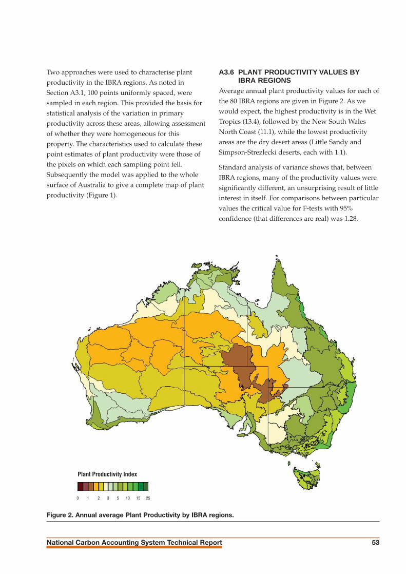
National Carbon Accounting System Technical Report 53
Two approaches were used to characterise plantproductivity in the IBRA regions. As noted inSection A3.1, 100 points uniformly spaced, weresampled in each region. This provided the basis forstatistical analysis of the variation in primaryproductivity across these areas, allowing assessmentof whether they were homogeneous for thisproperty. The characteristics used to calculate thesepoint estimates of plant productivity were those ofthe pixels on which each sampling point fell.Subsequently the model was applied to the wholesurface of Australia to give a complete map of plantproductivity (Figure 1).
A3.6 PLANT PRODUCTIVITY VALUES BYIBRA REGIONS
Average annual plant productivity values for each ofthe 80 IBRA regions are given in Figure 2. As wewould expect, the highest productivity is in the WetTropics (13.4), followed by the New South WalesNorth Coast (11.1), while the lowest productivityareas are the dry desert areas (Little Sandy andSimpson-Strezlecki deserts, each with 1.1).
Standard analysis of variance shows that, betweenIBRA regions, many of the productivity values weresignificantly different, an unsurprising result of littleinterest in itself. For comparisons between particularvalues the critical value for F-tests with 95%confidence (that differences are real) was 1.28.
Figure 2. Annual average Plant Productivity by IBRA regions.
Plant Productivity Index
0 1 2 3 5 10 15 25
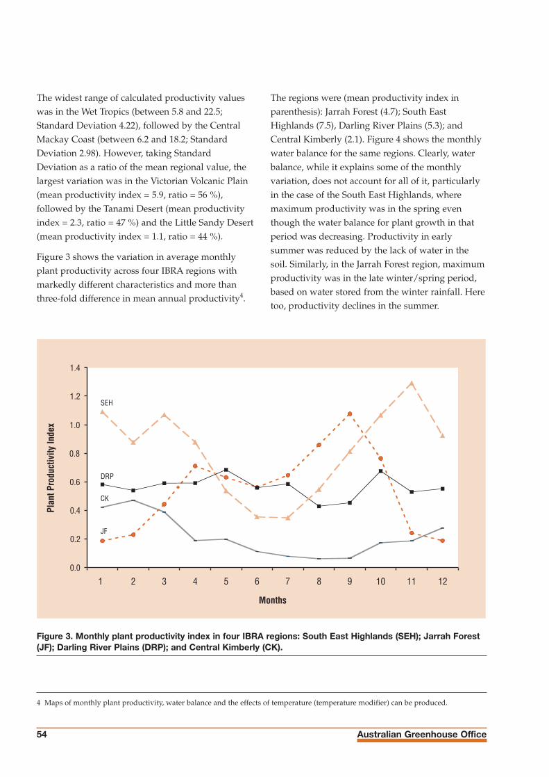
Australian Greenhouse Office54
The widest range of calculated productivity valueswas in the Wet Tropics (between 5.8 and 22.5;Standard Deviation 4.22), followed by the CentralMackay Coast (between 6.2 and 18.2; StandardDeviation 2.98). However, taking StandardDeviation as a ratio of the mean regional value, thelargest variation was in the Victorian Volcanic Plain(mean productivity index = 5.9, ratio = 56 %),followed by the Tanami Desert (mean productivityindex = 2.3, ratio = 47 %) and the Little Sandy Desert(mean productivity index = 1.1, ratio = 44 %).
Figure 3 shows the variation in average monthlyplant productivity across four IBRA regions withmarkedly different characteristics and more thanthree-fold difference in mean annual productivity4.
The regions were (mean productivity index inparenthesis): Jarrah Forest (4.7); South EastHighlands (7.5), Darling River Plains (5.3); andCentral Kimberly (2.1). Figure 4 shows the monthlywater balance for the same regions. Clearly, waterbalance, while it explains some of the monthlyvariation, does not account for all of it, particularlyin the case of the South East Highlands, wheremaximum productivity was in the spring eventhough the water balance for plant growth in thatperiod was decreasing. Productivity in earlysummer was reduced by the lack of water in thesoil. Similarly, in the Jarrah Forest region, maximumproductivity was in the late winter/spring period,based on water stored from the winter rainfall. Heretoo, productivity declines in the summer.
Figure 3. Monthly plant productivity index in four IBRA regions: South East Highlands (SEH); Jarrah Forest(JF); Darling River Plains (DRP); and Central Kimberly (CK).
DRP
1063
1.0
0.0
0.2
0.4
0.6
0.8
1.2
1.4
1 8 11 12
Months
Plan
t Pro
duct
ivity
Inde
x
JF
SEH
CK
2 4 5 7 9
4 Maps of monthly plant productivity, water balance and the effects of temperature (temperature modifier) can be produced.

National Carbon Accounting System Technical Report 55
A3.7 SPATIAL VARIATION IN PLANTPRODUCTIVITY WITHIN REGIONS
To assess the spatial variation of plant productivityacross IBRA regions, we plotted the standard errors(SEs) of the mean values obtained with varyingnumbers of samples for the two regions (Wet Tropicsand the Tanami) with the widest range in pointvalues. In both cases (Figs. 5a, 6a) the SE decreasedwith increasing numbers of sample points, butshowed little sign of reaching a steady value. Thespatial distribution of plant productivity values inthe two regions was quite different. In the WetTropics (Figure 5b) there was a fairly uniformdistribution of values, with a peak towards thehigher productivity end of the spectrum, while inthe Tanami (Figure 6b) the distribution was skewedstrongly left (towards the low productivity end of
the spectrum). There was little apparentrelationship between the spatial distribution of plantproductivity and the SE of the sample mean.
To evaluate the number of samples needed tominimise the SE of the mean, we took 300 samplepoints from each of the four regions (Jarrah Forest,South East Highlands, Darling River Plains, CentralKimberly) analysed earlier. The results are shown inFigures 7a, 8a, 9a and 10a, where the SEs are plottedagainst number of samples. The spatial distributionsof plant productivity are presented in Figures 7b,8b, 9b and 10b. The data indicate that, in mostcases, at least 200 sample points would need tobe analysed to minimise the SE of the mean value.Again, the spatial distribution of plant productivityvalues provides little guidance to the number ofsamples needed.
0
-80
-60
-40
-20
20
40
60
80
100
120
Months
Wat
er b
alan
ce (m
m/m
onth
)
JF
SEH
DRP
CK
1 2 5 7 9 11 12108643
Figure 4. Monthly water balance in the four IBRA regions for which plant productivity data are shown inFigure 3. Negative values indicate the dryness of the area but note that in the calculation of water balancesfor the model soil water content cannot go below zero.

Australian Greenhouse Office56
0
0.1
0.2
0.3
0.4
0.5
0.6
0.7
0 40 60 80 100
Number of samples
SE
of m
ean
ann.
pla
nt p
rodu
ctiv
ity
20
Wet Tropics
Figure 5a. (top) Change in the standard error of the mean productivity value with various numbers ofsample points, up to 100, in the Wet Topics region. There was no indication that a minimum value had beenreached. b. (bottom) Spatial distribution of plant productivity across the Wet Tropics region. The dataexhibit significant variation.
Nu
mbe
r of s
ampl
es
Plant Productivity Index Classes
0
2
4
6
8
10
12
14
16
18
20
22
24
26
28
<= 6 (6,8) (8,10) (10,12) (12,14) (14,16) (16,18) (18,20) (20,22) (22,24) > 24

National Carbon Accounting System Technical Report 57
Figure 6a. (top) Change in the standard error of the mean productivity value with various numbers ofsample points, up to 100, in the Tanami Desert region. There was no indication that a minimum value hadbeen reached. b. (bottom) Spatial distribution of mean annual plant productivity across the Tanami Desert.The data exhibit significant variation, with a marked peak in the low productivity range.
Nu
mbe
r of s
ampl
es
Plant Productivity Index Classes
0
3
6
9
12
15
18
21
24
27
30
<= 1 (1,1.5) (1.5,2) (2,2.5) (2.5,3) (3,3.5) (3.5,4) (4,4.5) > 4.5
0
0.05
0.1
0.15
0.2
0.25
0 20 40 60 80 100
Number of samples
SE o
f mea
n an
n. p
lant
pro
duct
ivity
Tanami Desert

Australian Greenhouse Office58
0
0.1
0.2
0.3
0.4
0.5
0 100 200 300
Number of samples
SE
of m
ean
ann
. pla
nt p
rodu
ctiv
ity
Jarrah Forest
Figure 7a. (top) Change in the standard error of the mean productivity value with various numbers ofsample points, up to 300, in the Jarrah Forest region. The curve indicates that 2-300 sample points wouldbe required to give an accurate value of the mean. b. (bottom) Spatial distribution of mean annual plantproductivity across the Jarrah Forest region. The curve is skewed towards lower values.
Nu
mbe
r of s
ampl
es
Plant Productivity Index Classes
(6.5,7)
0
2
4
6
8
10
12
14
16
18
20
22
24
26
28
30
<= 3 (3,3.5) (3.5,4) (4,4.5) (4.5,5) (5,5.5) (5.5,6) (6,6.5) (7,7.5) (7.5,8) > 8

National Carbon Accounting System Technical Report 59
Number of samples
SE o
f mea
n an
n. p
lant
pro
duct
ivity
0
0.1
0.2
0.3
0.4
0.5
0.6
0.7
0.8
0.9
0 50 100 150 200 250 300
South Eastern Highlands
Num
ber o
f sam
ples
Plant Productivity Index Classes
0
2
4
6
8
10
12
14
16
18
20
22
24
26
28
<= 0 (0,2) (2,4) (4,6) (6,8) (8,10) (10,12) (12,14) (14,16) > 16
Figure 8a. (top) Change in the standard error of the mean productivity value with various numbers ofsample points, up to 300, in the South Eastern Highlands. The curve indicates that 2-300 sample pointswould be required to give an accurate value of the mean. b. (bottom) Spatial distribution of mean annualplant productivity across the South Eastern Highlands region. The distribution is more uniform than inmost other regions.
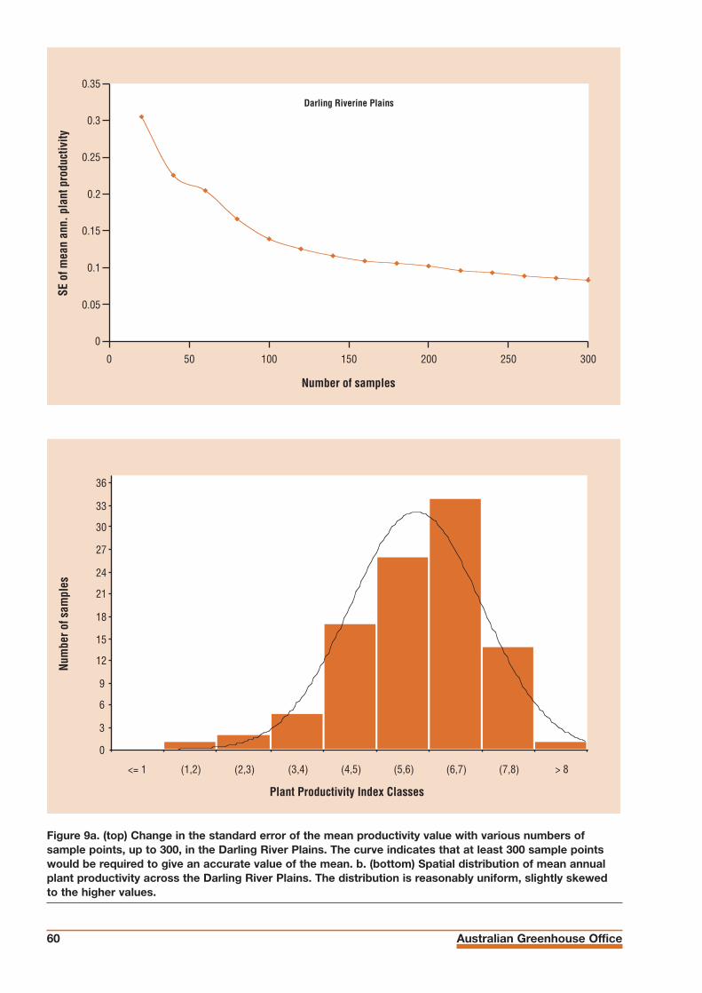
Australian Greenhouse Office60
Number of samples
SE o
f mea
n an
n. p
lant
pro
duct
ivity
Darling Riverine Plains
0
0.05
0.1
0.15
0.2
0.25
0.3
0.35
0 50 100 150 200 250 300
Nu
mbe
r of s
ampl
es
Plant Productivity Index Classes
0
3
6
9
12
15
18
21
24
27
30
33
36
<= 1 (1,2) (2,3) (3,4) (4,5) (5,6) (6,7) (7,8) > 8
Figure 9a. (top) Change in the standard error of the mean productivity value with various numbers ofsample points, up to 300, in the Darling River Plains. The curve indicates that at least 300 sample pointswould be required to give an accurate value of the mean. b. (bottom) Spatial distribution of mean annualplant productivity across the Darling River Plains. The distribution is reasonably uniform, slightly skewedto the higher values.

National Carbon Accounting System Technical Report 61
Number of samples
SE o
f mea
n an
n. p
lant
pro
duct
ivity
Central Kimberley
0
0.01
0.02
0.03
0.04
0.05
0.06
0.07
0.08
0.09
0 50 100 150 200 250 300
Num
ber o
f sam
ples
Plant Productivity Index Classes
0
3
6
9
12
15
18
21
24
27
30
33
36
<= 0.5 (0.5,1) (1,1.5) (1.5,2) (2,2.5) (2.5,3) (3,3.5) (3.5,4) > 4
Figure 10a. (top) Change in the standard error of the mean productivity value with varying numbersof sample points, up to 300, in the Central Kimberley region. The curve has not reached stable values;at least 300 sample points would be required to give an accurate value of the mean. b. (bottom) Spatialdistribution of mean annual plant productivity across the Central Kimberley region. The distribution isapproximately normal.

Australian Greenhouse Office62
A3.8 ANALYSIS OF PLANT PRODUCTIVITY BYCARNAHAN VEGETATION CLASSES
An analysis of productivity by Carnahan vegetation(present) classes was done by overlaying theCarnahan vegetation on the productivity surface.While the distribution of productivity values formost of the Carnahan vegetation classes shows that
there was a preferred value or niche, the range foreach vegetation class could be large. Figure 11shows the distribution of open woodland as shadedby the plant productivity index value. Due to thewide distribution of the open woodland vegetationclass it is not surprising that the productivity indexvalues have a range from 1 to 25.
Plant Productivity Index
0 1 2 3 5 10 15 25 No Data
Figure 11. The distribution of open woodland shaded by the plant productivity index value.

National Carbon Accounting System Technical Report 63
Figure 12 clearly shows the wide range of plantproductivity values for each vegetation class(e.g. open woodland ranges from a productivityindex of 1 to 20, open forest ranges from 2 to 20).It also clearly shows that the overlap between thevegetation classes is large and would not allow fordiscrimination of classes by plant productivity. Thiswill have implications for any stratification based onvegetation classes.
A3.9 CONCLUSIONSThe mean productivity values obtained for IBRAregions appear to be ‘reasonable’, insofar as theycorrespond well to vegetation and climatic regions.The method of calculation used here is based on thepremise that there is a linear relationship betweenthe PAR absorbed by vegetation and production.This is not linear over short periods (e.g. hours-days), and the use of the simple Beer’s Lawequation to calculate energy absorption by plantcanopies could lead to significant errors over suchperiods. However when we consider time periods aslong as a month, the assumption that biomassproduction is linearly related to biomass productionis justified (Landsberg et. al., 1997) and Beer’s Lawprovides good estimates of the energy absorbed.
0
20
40
60
80
100
1-1.5
1.5-2
2-2.5
2.5-3
3-4
4-5
5-7.5
7.5-10
10-12.5
12.5-15
15-20
20-25
closed open forest woodland open woodland scrub and heath
Perc
ent
Figure 12. Range of plant productivity values for the forest classes of present Carnahanvegetation classes.

Australian Greenhouse Office64
The full version of 3-PG (spatial) model has beenshown to provide good estimates of the productivityof forest types ranging from large, long-livedconifers (Coops et. al. 2001) to native forests in NewSouth Wales (Tickle et. al. 2001) and fast-growingeucalypt plantations in Brazil (A.C. de Almeida andJ.J.Landsberg; unpublished data). The model hasalso been tested against biomass measurementsmade in New Zealand re-growth scrub (White et. al.,2000; Neal Scott, Landcare NZ; pers. comm.) andwas found to perform well. These examples showthat, given appropriate inputs, the basic modelprovides good estimates of productivity for specificlocations, allowing confidence in the model as anestimator of wide-scale productivity values.
The spatial variation in plant productivity across theIBRA regions indicates that, whatever their value interms of ecological regions and guides for theestablishment of reserves, these regions are nothomogeneous in terms of productivity. It is clearthat the IBRA regions not only contain a variety ofsoil types – which would have been impossible toavoid – but, in most cases, they lay across theboundaries of several quite different climaticregions. This would explain some of the variancethat needs to be able to be taken into account whenmaking calculations for specific locations.
A3.10 FOLLOW UP RESEARCHUltimately, a variant of the 3-PG model (as usedhere in these preliminary investigations, followingLandsberg et. al. 1997) was used as the productivitymodel, in addition to the long-term average plantproduction index and top soil moisture deficits forthe NCAS (as fully described in the main body ofthis report). Annual plant productivity indices werealso subsequently used in development of the fullcarbon accounting model for the NCAS (seeRichards 2001).
A3.11 RELEVANT CITATIONS Coops, N.C., Waring, R.H., Brown, S.R. & Running,
S.W. 2001. Comparisons of Predictions of Net Primary
Production and Seasonal Patterns in Water Use
Derived with Two Forest Growth Models in
Southwestern Oregon. Ecological Modelling.142:61-81.
Landsberg, J.J. 1986. Coupling of carbon, water and
nutrient interactions in woody plant soil systems.
Tree Physiology 2.
Landsberg, J.J. & Gower, S.T. 1997. Applications of
Physiological Ecology to Forest Management.
Academic Press: San Diego Press. 354pp.
Landsberg, J.J. & Waring, R.H. 1997. A generalised
model of forest productivity using simplified concepts
of radiation-use efficiency, carbon balance and
partitioning. Forest Ecology and Management95:209–228.
Landsberg, J.J., Prince, S.D., Jarvis, P.G., McMurtrie,R.E., Luxmoore, R. & Medlyn, B.E. 1997. Energy
conversion and use in forests: An analysis of forest
production in terms of radiation utilisation efficiency.
In The Use of Remote Sensing in the Modeling ofForest Productivity at Scales from the Stand to theGlobe. Eds: Gholz, H.L., Nakane, K., & Shimoda,H. Kluwer Academic Publishers: Dordrecht.
McKenzie, N.J., Jacquier, D.W., Ashton, L.J. &Cresswell, H.P. 2000. Estimation of Soil Properties
Using the Atlas of Australian Soils. CSIRO Landand Water Technical Report 11/00, February 2000.
McMurtrie, R.E., Gholz, H.L., Linder, S. & Gower,S.T. 1994. Climatic factors controlling the productivity
of pine stands: A model-based analysis. EcologicalBulletins 43:173–188.
Potter, C.S., Randerson, J.T., Field, C.B., Matson,P.A., Vitousek, P.M., Mooney, H.A. & Klooster,S.A. 1993. Terrestrial ecosystem production: A process
model based on global satellite and surface data.
Global Biogeochemical Cycles 7:811–841.

National Carbon Accounting System Technical Report 65
Richards, G.P. 2001. The FullCAM Carbon Accounting
Model: Development, Calibration and Implementation
for the National Carbon Accounting System. NationalCarbon Accounting System Technical ReportNo. 28, Australian Greenhouse Office,Canberra, pp49.
Ruimey, A., Saugier, B. & Dedieu, G. 1994.Methodology for the estimation of terrestrial net
primary production from remotely sensed data.
J. Geophys. Res. 99:5263–5283.
Thackway, R. & Cresswell, I.D. (Eds). 1995. An
Interim Biogeographic Regionalisation for Australia:
A Framework for Establishing the National System of
Reserves, Version 4.0. Australian NatureConservation Agency, Canberra.http://www.environment.gov.au/bg/nrs/ibraimcr/ibra_95/
Tickle, P.K., Coops, N.C. & Hafner, S.D. 2001.Assessing Forest Productivity at Local Scales Across a
Native Eucalypt Forest Using a Process Model, 3PG-
SPATIAL. Forest Ecology and Management.152:275-291.
White, J.D., Coops, N.C. & Scott, N.A. 2000Predicting broad-scale forest and scrub biomass for
New Zealand: Investigating the application of a
physiologically-based model. Ecological Modeling131: 175–190.
A4. FOREST GROWTH DATA
URS Australia
Compiled forest growth data tables arepresented overleaf.

Australian Greenhouse Office66
Site
Info
rmat
ion
(Sou
th A
ustra
lia, H
assa
ll &
Ass
ocia
tes,
199
9a)
Biom
ass
MAI
Plan
ting
Volu
me
Site
Fac
tors
Esta
blis
hmen
t & S
tand
Man
agem
ent
ID
Nam
e, L
ocat
ion,
Es
t.Ar
ea
Spec
ies
List
&t/h
aAg
et/h
a/yr
Dens
ity
m3 /h
ae.
g. ra
infa
ll, s
oil t
ype/
qual
ity,
e.g.
site
pre
para
tion
and
prio
r lan
duse
, tub
esto
ck/
Coor
dina
tes
Plan
ted
Purp
ose
(tree
s/ha
)to
pogr
aphy
, acc
ess
to w
ater
, sal
inity
dire
ct s
eed,
wee
ds/d
isea
se/p
ests
, fire
, irr
igat
ion
1Hy
nam
Par
k,
1990
-E.
cam
aldu
lens
is,
88.0
318
11.0
0-
N/A
Low
er S
outh
Eas
tE.
leuc
oxyl
on,
66.0
22
E. o
ccid
enta
llis
Lat/l
ong:
365
713,
140
5244
Shel
terb
elt
2St
ruan
Fai
rlam
b,
1993
0.7
haE.
ova
ta,
4.76
15
0.95
1,08
9N/
ALo
wer
Sou
th E
ast
E. o
ccid
enta
lis,
3.57
2
Allo
casu
arin
aLa
t/lon
g: 3
6062
2,14
0453
4ve
rtici
llate
Purp
ose
not
spec
ified
3St
ruan
Roa
dsid
e,
1990
0.9
haE.
vim
inal
is96
.191
812
.02
-N/
ALo
wer
Sou
th E
ast
E. le
ucox
ylon
,72
.142
Acac
ia
Lat/l
ong:
370
620,
140
4729
pycn
anth
a
Purp
ose
not
spec
ified
4M
ark
Mor
ris,
1993
2.5
haE.
cne
orifo
lia,
18.2
915
3.66
-N/
AKa
ngar
oo Is
land
E. d
iver
sifo
lia,
13.7
2
E. c
osm
ophy
llaLa
t/lon
g: 3
5491
1, 1
3742
11Gr
ound
wat
erre
char
ge/s
alin
ity
cont
rol
Rain
fall:
Av
558
mm
Soil:
Bla
ck re
ndzin
a so
ils w
ith a
nim
perv
ious
lim
esto
ne la
yer a
t 30
cm,
pH7.
0 at
sur
face
to 8
.5 a
t 30
cm
Topo
grap
hy: F
lat p
lain
Wat
er: R
ainf
ed, d
epth
togr
ound
wat
erun
know
n.
Rain
fall:
Av
558
mm
Soil:
San
dy c
lay
loam
ove
r cla
y Te
rra
Ross
a, p
H 6.
0 at
sur
face
to 7
.0 a
t 30
cm
Topo
grap
hy: N
ot s
peci
fied
Wat
er: R
ainf
ed, d
epth
togr
ound
wat
erun
know
n.
Rain
fall:
Av
532
mm
Soil:
Cla
y lo
am o
ver c
lay,
pH
6.0
atsu
rfac
e to
7.0
at 5
0 cm
Topo
grap
hy: N
ot s
peci
fied
Wat
er: R
ainf
ed, d
epth
togr
ound
wat
erun
know
n.
Rain
fall:
Av
581
mm
Soil:
San
dy lo
am o
ver c
lay,
pH
5.5
atsu
rfac
e to
7.0
at 5
0 cm
Topo
grap
hy: F
lat p
lain
Wat
er: R
ainf
ed, a
djac
ent t
o da
iry fa
rmw
hich
may
or m
ay n
ot b
e irr
igat
ed(u
nspe
cifie
d). D
epth
togr
ound
wat
erun
know
n.
Site
pre
para
tion
unkn
own.
Pre
viou
sly
used
for
shee
p gr
azin
g.
Tube
stoc
k.
No th
inni
ngs.
Som
e in
cide
nce
of p
ests
(spi
tfire
cat
epill
ars)
and
wee
ds. N
o tre
atm
ent.
No o
ther
pro
blem
s.
Rain
fed
only.
Site
pre
para
tion
unkn
own.
Pre
viou
s us
e un
know
n.
Dire
ct s
eedi
ng.
Thin
ning
s hi
stor
y no
t spe
cifie
d.
Som
e in
cide
nce
of in
sect
atta
ck a
nd w
eeds
,bu
tno
dam
age.
Som
e st
unte
d gr
owth
due
tocr
owdi
ng o
ut. N
o ot
her p
robl
ems.
Rain
fed
only.
Site
pre
para
tion
unkn
own.
Pre
viou
sly
used
for
dairy
gra
zing.
Dire
ct s
eedi
ng.
Sele
ctiv
e th
inni
ngs
for f
irew
ood.
Som
e st
unte
d gr
owth
due
to c
row
ding
out
.No
othe
r pro
blem
s as
soci
ated
with
wee
ds/d
isea
se/p
ests
, dro
ught
or f
ire.
No h
isto
ry o
f irr
igat
ion
on th
e tre
es o
r in
the
adja
cent
dai
ry p
astu
re is
spe
cifie
d.
Site
pre
para
tion
unkn
own.
Pre
viou
s us
em
ixed
farm
ing.
Dire
ct s
eedi
ng.
Thin
ning
s hi
stor
y no
t spe
cifie
d.
No p
robl
ems
asso
ciat
ed w
ith w
eeds
/dis
ease
/pes
ts,
drou
ght o
r fire
.
Rain
fed
only.
A4
- Ta
ble
1a.
Gro
wth
Dat
a fo
r S
ites
in S
out
h A
ustr
alia
, Has
sall
& A
sso
ciat
es (
1999
a)
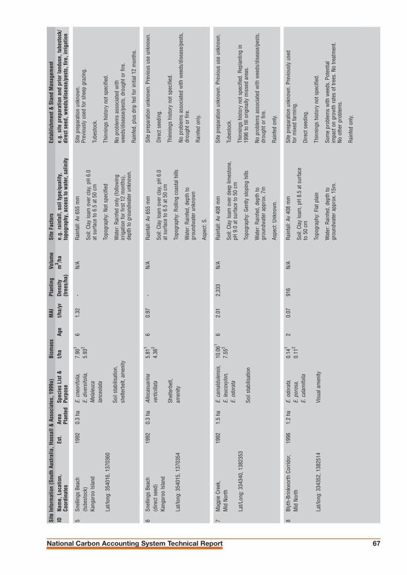
National Carbon Accounting System Technical Report 67
5Sn
ellin
gs B
each
19
920.
3 ha
E. c
neor
ifolia
,7.
901
61.
32-
N/A
(tube
stoc
k)E.
div
ersi
folia
,5.
932
Kang
aroo
Isla
ndM
elal
euca
la
nceo
lata
Lat/l
ong:
354
016,
137
0360
Soil
stab
ilisa
tion,
shel
terb
elt,
amen
ity
6Sn
ellin
gs B
each
19
920.
3 ha
Allo
casu
arin
a5.
811
60.
97-
N/A
(dire
ct s
eed)
verti
cilla
ta4.
362
Kang
aroo
Isla
ndSh
elte
rbel
t,La
t/lon
g: 3
5401
5, 1
3703
54am
enity
7M
agpi
e Cr
eek,
19
921.
5 ha
E. c
amal
dule
nsis
,10
.061
62.
012,
333
N/A
Mid
Nor
thE.
leuc
oxyl
on,
7.55
2
E. o
dora
taLa
t/Lon
g: 3
3434
0, 1
3823
53So
il st
abili
satio
n
8Bl
yth-
Brin
kwor
th C
orrid
or,
1996
1.2
haE.
odo
rata
, 0.
141
20.
0791
6N/
AM
id N
orth
E. p
oros
a,
0.11
2
E. c
alam
ifolia
Lat/l
ong:
334
352,
138
2514
Visu
al a
men
ity
Site
Info
rmat
ion
(Sou
th A
ustra
lia, H
assa
ll &
Ass
ocia
tes,
199
9a)
Biom
ass
MAI
Plan
ting
Volu
me
Site
Fac
tors
Esta
blis
hmen
t & S
tand
Man
agem
ent
ID
Nam
e, L
ocat
ion,
Es
t.Ar
ea
Spec
ies
List
&t/h
aAg
et/h
a/yr
Dens
ity
m3 /h
ae.
g. ra
infa
ll, s
oil t
ype/
qual
ity,
e.g.
site
pre
para
tion
and
prio
r lan
duse
, tub
esto
ck/
Coor
dina
tes
Plan
ted
Purp
ose
(tree
s/ha
)to
pogr
aphy
, acc
ess
to w
ater
, sal
inity
dire
ct s
eed,
wee
ds/d
isea
se/p
ests
, fire
, irr
igat
ion
Rain
fall:
Av
655
mm
Soil:
Cla
y lo
am o
ver c
lay,
pH
6.0
atsu
rfac
e to
6.5
at 5
0 cm
Topo
grap
hy: N
ot s
peci
fied
Wat
er: R
ainf
ed o
nly
(follo
win
girr
igat
ion
for f
irst 1
2 m
onth
s),
dept
hto
grou
ndw
ater
unk
now
n.
Site
pre
para
tion
unkn
own.
Prev
ious
lyus
edfo
rshe
ep g
razin
g.
Tube
stoc
k.
Thin
ning
s hi
stor
y no
t spe
cifie
d.
No p
robl
ems
asso
ciat
ed w
ithw
eeds
/dis
ease
/pes
ts,d
roug
ht o
r fire
.
Rain
fed,
plu
s dr
ip fe
d fo
r ini
tial 1
2 m
onth
s.
Rain
fall:
Av
655
mm
Soil:
Cla
y lo
am o
ver c
lay,
pH
6.0
atsu
rfac
e to
6.5
at 5
0 cm
Topo
grap
hy: R
ollin
g co
asta
l hill
s
Wat
er: R
ainf
ed, d
epth
togr
ound
wat
erun
know
n
Aspe
ct: S
.
Site
pre
para
tion
unkn
own.
Pre
viou
s us
e un
know
n.
Dire
ct s
eedi
ng.
Thin
ning
s hi
stor
y no
t spe
cifie
d.
No p
robl
ems
asso
ciat
ed w
ith w
eeds
/dis
ease
/pes
ts,
drou
ght o
r fire
.
Rain
fed
only.
Site
pre
para
tion
unkn
own.
Pre
viou
s us
e un
know
n.
Tube
stoc
k.
Thin
ning
s hi
stor
y no
t spe
cifie
d. R
epla
ntin
g in
1996
to fi
ll or
igin
ally
mis
sed
area
s.
No p
robl
ems
asso
ciat
ed w
ith w
eeds
/dis
ease
/pes
ts,
drou
ght o
r fire
.
Rain
fed
only.
Rain
fall:
Av
408
mm
Soil:
Cla
y lo
am o
ver d
eep
limes
tone
,pH
9.0
at s
urfa
ce to
50
cm
Topo
grap
hy: G
ently
slo
ping
hill
s
Wat
er: R
ainf
ed, d
epth
togr
ound
wat
erap
prox
. 7m
Aspe
ct: U
nkno
wn.
Site
pre
para
tion
unkn
own.
Pre
viou
sly
used
form
ixed
farm
ing.
Dire
ct s
eedi
ng.
Thin
ning
s hi
stor
y no
t spe
cifie
d.
Som
e pr
oble
ms
with
wee
ds. P
oten
tial
impa
cton
grow
th ra
tes
of tr
ees.
No
treat
men
t.No
othe
rpro
blem
s.
Rain
fed
only.
Rain
fall:
Av
408
mm
Soil:
Cla
y lo
am, p
H 8.
5 at
sur
face
to50
cm
Topo
grap
hy: F
lat p
lain
Wat
er: R
ainf
ed, d
epth
togr
ound
wat
erap
prox
. 15m
.
Australian Greenhouse Office68
9Bl
yth,
19
962.
5 ha
E. o
dora
ta,
0.18
12
0.09
833
N/A
Mid
Nor
thAl
loca
suar
ina
0.14
2
verti
cilla
ta,
Lat/l
ong:
334
957,
138
2859
Acac
ia p
ycna
ntha
Visu
al a
men
ity
10M
ouril
ya
1992
1 ha
E. c
lado
caly
x,
6.34
16
1.06
-N/
A(d
irect
see
d)Ac
acia
pyc
nant
ha4.
752
Eyre
Pen
insu
laAl
loca
suar
ina
verti
cilla
ta,
Lat/l
ong:
343
612,
135
4336
Purp
ose
not s
peci
fied
11M
ouril
ya
1994
2 ha
E. c
lado
caly
x,7.
531
41.
88-
N/A
(tube
stoc
k)E.
lans
dow
nean
a5.
642
Eyre
Pen
insu
lava
r. al
bopu
rpur
eaE.
leuc
oxyl
onLa
t/lon
g: 3
4345
3, 1
3543
36Sh
elte
rbel
t
12W
arro
w,
1992
2.5
haE.
incr
assa
ta,
5.35
16
0.89
-N/
AEy
re P
enin
sula
E. p
oros
a,4.
012
Allo
casu
arin
aLa
t/lon
g: 3
4185
5, 1
3528
40ve
rticl
lata
Habi
tat
Site
Info
rmat
ion
(Sou
th A
ustra
lia, H
assa
ll &
Ass
ocia
tes,
199
9a)
Biom
ass
MAI
Plan
ting
Volu
me
Site
Fac
tors
Esta
blis
hmen
t & S
tand
Man
agem
ent
ID
Nam
e, L
ocat
ion,
Es
t.Ar
ea
Spec
ies
List
&t/h
aAg
et/h
a/yr
Dens
ity
m3 /h
ae.
g. ra
infa
ll, s
oil t
ype/
qual
ity,
e.g.
site
pre
para
tion
and
prio
r lan
duse
, tub
esto
ck/
Coor
dina
tes
Plan
ted
Purp
ose
(tree
s/ha
)to
pogr
aphy
, acc
ess
to w
ater
, sal
inity
dire
ct s
eed,
wee
ds/d
isea
se/p
ests
, fire
, irr
igat
ion
Rain
fall:
Av
427
mm
Soil:
Cla
y lo
am, p
H ap
prox
. 8.0
Topo
grap
hy: F
lat p
lain
Wat
er: R
ainf
ed, d
epth
togr
ound
wat
er10
-15m
.
Rain
fall:
Av
495
mm
Soil:
San
dy lo
am, p
H ap
prox
. 6.5
Topo
grap
hy: G
ently
slo
ping
low
hill
s
Wat
er: R
ainf
ed, d
epth
togr
ound
wat
er10
-15m
Aspe
ct: S
.
Rain
fall:
Av
424
mm
Soil:
San
dy lo
am o
ver c
lay,
pH
unkn
own
Topo
grap
hy: G
ently
slo
ping
low
hill
s
Wat
er: R
ainf
ed, d
epth
togr
ound
wat
er5m
Aspe
ct: S
.
Rain
fall:
Av
420
mm
Soil:
San
d ov
er li
mes
tone
, pH
7.5
atsu
rfac
e to
8.5
-9.0
at 3
0-40
cm
Topo
grap
hy: F
lat p
lain
- ge
ntle
slo
pe
Wat
er: R
ainf
ed, d
epth
togr
ound
wat
er3m
Aspe
ct: S
W.
Site
pre
para
tion
unkn
own.
Pre
viou
sly
used
as
ara
ilway
cor
ridor
.
Dire
ct s
eedi
ng.
No T
hinn
ings
.
Sign
ifica
nt w
eed
infe
stat
ion
requ
iring
trea
tmen
t.No
oth
er p
robl
ems.
Rain
fed
only.
Site
pre
para
tion
unkn
own.
Pre
viou
s us
e un
know
n.
Dire
ct s
eedi
ng.
Thin
ning
s hi
stor
y un
know
n.
No p
robl
ems
asso
ciat
ed w
ithw
eeds
/dis
ease
/pes
ts,d
roug
ht o
r fire
.
Rain
fed
only.
Site
pre
para
tion
unkn
own.
Pre
viou
sly
used
for
mix
ed fa
rmin
g.
Tube
stoc
k.
Thin
ning
s hi
stor
y un
know
n.
No p
robl
ems
asso
ciat
ed w
ith w
eeds
/dis
ease
/pes
ts,
drou
ght o
r fire
.
Rain
fed
only.
Site
pre
para
tion
unkn
own.
Pre
viou
sly
used
for
graz
ing.
Dire
ct s
eedi
ng.
Thin
ning
s hi
stor
y un
know
n.
No p
robl
ems
asso
ciat
ed w
ith w
eeds
/dis
ease
/pes
ts,
drou
ght o
r fire
.
Rain
fed
only.
A4
- Ta
ble
1a.
Gro
wth
Dat
a fo
r S
ites
in S
out
h A
ustr
alia
, Has
sall
& A
sso
ciat
es (
1999
a) c
ont
inue
d.
National Carbon Accounting System Technical Report 69
13Ja
ckso
n19
90-
E. g
raci
lis,
133.
371
816
.67
-N/
A(d
irect
see
d)E.
leuc
oxyl
on,
100.
032
Uppe
r Sou
th E
ast
E. le
ptop
hylla
Lat/l
ong:
362
251,
140
1934
Purp
ose
not s
peci
fied
14Ja
ckso
n19
880.
6 ha
E. g
raci
lis,
15.2
1110
1.52
-N/
A(tu
best
ock)
E.
fasc
icul
osa,
11.4
02
Uppe
r Sou
th E
ast
E. c
amal
dule
nsis
Lat/l
ong:
362
248,
140
1934
Purp
ose
not s
peci
fied
15M
enin
gie-
Coon
alpy
n Ro
ad,
1993
-E.
leuc
oxyl
on,
10.7
715
2.15
-N/
AUp
per S
outh
Eas
tAl
loca
suar
ina
8.08
2
verti
cilla
ta,
Lat/l
ong:
354
132,
139
2646
Allo
casu
arin
am
uelle
riana
Road
side
she
lterb
elt,
reve
geta
tion
trial
16De
l Fab
bro,
19
410
ha
Mel
aleu
ca
6.89
14
1.72
-N/
AUp
per S
outh
Eas
tbr
evifo
lia5.
162
Mel
aleu
ca
Lat/l
ong:
363
921,
140
1708
halm
atur
orum
E. le
ucox
ylon
Grou
ndw
ater
rech
arge
/sa
linity
con
trol
Rain
fall:
Av
560
mm
Soil:
San
d ov
er s
hallo
w c
lay,
pH
6.0
atsu
rfac
e to
7.0
at 5
0 cm
Topo
grap
hy: R
ollin
g pl
ains
Wat
er: R
ainf
ed, d
epth
togr
ound
wat
erun
know
n.
Site
pre
para
tion
unkn
own.
Pre
viou
s us
e un
know
n.
Dire
ct s
eedi
ng.
Thin
ning
s hi
stor
y un
know
n.
No p
robl
ems
asso
ciat
ed w
ithw
eeds
/dis
ease
/pes
ts,d
roug
ht o
r fire
.
Rain
fed
only.
Site
Info
rmat
ion
(Sou
th A
ustra
lia, H
assa
ll &
Ass
ocia
tes,
199
9a)
Biom
ass
MAI
Plan
ting
Volu
me
Site
Fac
tors
Esta
blis
hmen
t & S
tand
Man
agem
ent
ID
Nam
e, L
ocat
ion,
Es
t.Ar
ea
Spec
ies
List
&t/h
aAg
et/h
a/yr
Dens
ity
m3 /h
ae.
g. ra
infa
ll, s
oil t
ype/
qual
ity,
e.g.
site
pre
para
tion
and
prio
r lan
duse
, tub
esto
ck/
Coor
dina
tes
Plan
ted
Purp
ose
(tree
s/ha
)to
pogr
aphy
, acc
ess
to w
ater
, sal
inity
dire
ct s
eed,
wee
ds/d
isea
se/p
ests
, fire
, irr
igat
ion
Rain
fall:
Av
560
mm
Soil:
San
d, lo
w s
alin
ity, p
H 6.
0-6.
5 at
surf
ace
to 7
.0-8
.5 a
t 50
cm
Topo
grap
hy: R
ollin
g pl
ains
Wat
er: R
ainf
ed, d
epth
togr
ound
wat
erun
know
n.
Site
pre
para
tion
unkn
own.
Pre
viou
s us
e un
know
n.
Tube
stoc
k.
Thin
ning
s hi
stor
y un
know
n.
No p
robl
ems
asso
ciat
ed w
ithw
eeds
/dis
ease
/pes
ts,d
roug
ht o
r fire
.
Rain
fed
only.
Rain
fall:
Av
468
mm
Soil:
Non
-wet
ting
sand
, low
sal
inity
,pH
8.0
at s
urfa
ce to
9.0
at 5
0 cm
Topo
grap
hy: F
lat p
lain
Wat
er: R
ainf
ed, d
epth
togr
ound
wat
erun
know
n.
Site
pre
para
tion
unkn
own.
Pre
viou
s us
e un
know
n.
Dire
ct s
eedi
ng.
Thin
ning
s hi
stor
y un
know
n.
No p
robl
ems
asso
ciat
ed w
ith w
eeds
/dis
ease
/pes
ts,
drou
ght o
r fire
.
Rain
fed
only.
Rain
fall:
Av
521
mm
Soil:
Poo
r san
ds o
ver c
lay,
evi
denc
e of
salin
ity, p
H 6.
0
Topo
grap
hy: R
ollin
g pl
ain
Wat
er: R
ainf
ed, p
lus
shal
low
dep
th to
wat
erta
ble,
par
ticul
arly
in w
inte
r mon
ths.
Site
fenc
ed o
ff an
d sp
raye
d fo
r wee
ds p
rior t
oso
win
g. P
revi
ousl
y us
ed a
s sh
eep
graz
ing.
Dire
ct s
eedi
ng.
No th
inni
ngs.
No p
robl
ems
asso
ciat
ed w
ith w
eeds
/dis
ease
/pes
ts,
drou
ght o
r fire
.
Rain
fed,
plu
s ac
cess
to s
hallo
w g
roun
dwat
er.

Australian Greenhouse Office70
17La
ngho
rne
Cree
k Ce
met
ery,
1992
-E.
leuc
oxyl
on,
10.3
616
1.73
-N/
AM
urra
ylan
dsAc
acia
pyc
nant
ha,
7.77
2
Acac
iaLa
t/lon
g: 3
5174
9, 1
3903
12br
achy
botr
ya
Seed
col
lect
ion
18Ha
rtley
Dum
p,19
92-
E. le
ucox
ylon
,5.
261
60.
88-
N/A
Mur
rayl
ands
E. p
oros
a,3.
942
Acac
ia c
alam
ifolia
Lat/l
ong:
351
111,
139
0205
Site
reha
bilit
atio
n
19Sw
anpo
rt,19
91-
E. le
ucox
ylon
spp
.24
.171
73.
45-
N/A
Mur
rayl
ands
leuc
oxyl
on,
18.1
32
E. le
ucox
ylon
La
t/lon
g: 3
5085
5, 1
3918
42sp
p. s
teph
enae
,E.
por
osa
Purp
ose
not s
peci
fied
20Hu
gh L
ongb
otto
m,
1992
0.9
haE.
por
osa,
11
.511
61.
92-
N/A
York
e Pe
nins
ula
Acac
ia p
ycna
ntha
,8.
632
Acac
ia n
otab
ilis
Lat/l
ong:
342
137,
137
3235
Shel
terb
elt
Rain
fall:
Av
392
mm
Soil:
Cla
y w
ith v
aryi
ng le
vels
of
limes
tone
, pH
8.0
at s
urfa
ce to
9.0
at30
cm
Topo
grap
hy: G
ently
rolli
ng h
ills
Wat
er: R
ainf
ed, d
epth
tow
ater
tabl
eun
know
n.
Site
pre
para
tion
unkn
own.
Adj
oini
ng ru
bbis
hdu
mp/
quar
ry.
Dire
ct s
eedi
ng.
Thin
ning
s hi
stor
y un
know
n.
No p
robl
ems
asso
ciat
ed w
ithw
eeds
/dis
ease
/pes
ts, d
roug
ht o
r fire
.
Rain
fed
only.
Site
Info
rmat
ion
(Sou
th A
ustra
lia, H
assa
ll &
Ass
ocia
tes,
199
9a)
Biom
ass
MAI
Plan
ting
Volu
me
Site
Fac
tors
Esta
blis
hmen
t & S
tand
Man
agem
ent
ID
Nam
e, L
ocat
ion,
Es
t.Ar
ea
Spec
ies
List
&t/h
aAg
et/h
a/yr
Dens
ity
m3 /h
ae.
g. ra
infa
ll, s
oil t
ype/
qual
ity,
e.g.
site
pre
para
tion
and
prio
r lan
duse
, tub
esto
ck/
Coor
dina
tes
Plan
ted
Purp
ose
(tree
s/ha
)to
pogr
aphy
, acc
ess
to w
ater
, sal
inity
dire
ct s
eed,
wee
ds/d
isea
se/p
ests
, fire
, irr
igat
ion
Rain
fall:
Av
392
mm
Soil:
Cla
y w
ith in
crea
sing
leve
ls o
flim
esto
ne a
t 50
cm, p
H 6.
0-6.
5 at
surf
ace
to 7
.5-8
.5 a
t 50
cm
Topo
grap
hy: L
ow g
ently
slo
ping
hill
side
Wat
er: R
ainf
ed, d
epth
to w
ater
tabl
eap
prox
. 3m
.
Site
pre
para
tion
unkn
own.
Pre
viou
sly
used
for
dairy
farm
ing
and
crop
ping
.
Dire
ct s
eedi
ng.
Thin
ning
s of
low
er li
mbs
and
infe
rior s
aplin
gs.
No p
robl
ems
asso
ciat
ed w
ithw
eeds
/dis
ease
/pes
ts, d
roug
ht o
r fire
.
Rain
fed,
plu
s po
ssib
le a
cces
s to
gro
undw
ater
.
Rain
fall:
Av
346
mm
Soil:
San
d, lo
w s
alin
ity, p
H 7.
0 at
sur
face
to 8
.0-8
.5 a
t 50
cm
Topo
grap
hy: G
ently
und
ulat
ing
Wat
er: R
ainf
ed, d
epth
to
wat
erta
ble
7-10
m
Aspe
ct: W
.
Site
pre
para
tion
unkn
own.
Pre
viou
sly
used
fora
gric
ultu
ral p
urpo
ses.
Tube
stoc
k.
Thin
ning
s hi
stor
y un
know
n.
Som
e pr
oble
ms
asso
ciat
ed w
ith w
eeds
and
rabb
itsw
hich
may
be
affe
ctin
g gr
owth
. No
othe
rpro
blem
s.
Rain
fed
only.
Rain
fall:
Av
504
mm
Soil:
Cla
y-lo
am, p
H un
know
n
Topo
grap
hy: G
ently
rolli
ng p
lain
Wat
er: R
ainf
ed, d
epth
tow
ater
tabl
eun
know
n.
Site
pre
para
tion
unkn
own.
Pre
viou
sly
used
for
crop
ping
.
Dire
ct s
eedi
ng.
Thin
ning
s hi
stor
y un
know
n.
No p
robl
ems
asso
ciat
ed w
ith w
eeds
/dis
ease
/pes
ts,
drou
ght o
r fire
.
Rain
fed
only.
A4
- Ta
ble
1a.
Gro
wth
Dat
a fo
r S
ites
in S
out
h A
ustr
alia
, Has
sall
& A
sso
ciat
es (
1999
a) c
ont
inue
d.

National Carbon Accounting System Technical Report 71
Site
Info
rmat
ion
(Sou
th A
ustra
lia, H
assa
ll &
Ass
ocia
tes,
199
9a)
Biom
ass
MAI
Plan
ting
Volu
me
Site
Fac
tors
Esta
blis
hmen
t & S
tand
Man
agem
ent
ID
Nam
e, L
ocat
ion,
Es
t.Ar
ea
Spec
ies
List
&t/h
aAg
et/h
a/yr
Dens
ity
m3 /h
ae.
g. ra
infa
ll, s
oil t
ype/
qual
ity,
e.g.
site
pre
para
tion
and
prio
r lan
duse
, tub
esto
ck/
Coor
dina
tes
Plan
ted
Purp
ose
(tree
s/ha
)to
pogr
aphy
, acc
ess
to w
ater
, sal
inity
dire
ct s
eed,
wee
ds/d
isea
se/p
ests
, fire
, irr
igat
ion
21M
aitla
nd-M
inla
ton
Road
,19
940.
6 ha
E. p
oros
a,2.
101
40.
52-
N/A
York
e Pe
nins
ula
Acac
ia s
pine
scen
s,1.
572
Dode
naea
vis
cosa
Lat/l
ong:
342
637,
137
3920
Road
side
re
vege
tatio
n tri
al
22Kl
opp,
19
900.
27 h
aE.
por
osa,
22
.561
82.
82-
N/A
York
e Pe
nins
ula
E. s
ocia
lis,
16.9
22
E. c
alyc
ogon
aLa
t/lon
g: 3
4285
5, 1
3745
20Ro
adsi
de p
lant
ing
23M
ount
Bar
ker T
anne
ry,
1992
12 h
aE.
vim
inal
is,
30.3
016
5.05
-N/
AM
ount
Lof
ty R
ange
sE.
leuc
oxyl
on,
22.7
22
E. fa
scic
ulos
a
Lat/l
ong:
350
332,
138
5151
Site
reha
bilit
atio
n,
amen
ity
24Fl
axle
y Ho
listic
Tra
ding
, 19
915
haE.
fasc
icul
osa,
97.5
517
13.9
4-
N/A
Mou
nt L
ofty
Ran
ges
E. o
bliq
ua,
73.1
72
Acac
ia
Lat/l
ong:
350
820,
138
4950
mel
anox
ylon
Reve
geta
tion
Rain
fall:
Av
504
mm
Soil:
Cla
y-lo
am, p
H un
know
n
Topo
grap
hy: G
ently
rolli
ng p
lain
Wat
er: R
ainf
ed, d
epth
tow
ater
tabl
eun
know
n.
Site
pre
para
tion
unkn
own.
Pre
viou
s us
eno
tspe
cifie
d.
Dire
ct s
eedi
ng.
Thin
ning
s hi
stor
y un
know
n.
No p
robl
ems
asso
ciat
ed w
ithw
eeds
/dis
ease
/pes
ts,d
roug
ht o
r fire
.
Rain
fed
only.
Rain
fall:
Av
414
mm
Soil:
San
dy lo
am, p
H 8.
5 at
sur
face
to9.
0 at
50
cm
Topo
grap
hy: R
ollin
g pl
ains
Wat
er: R
ainf
ed, d
epth
to w
ater
tabl
eun
know
n bu
t bel
ieve
d to
sea
sona
lly b
ew
ithin
root
zon
e
Aspe
ct: N
.
Site
pre
para
tion
unkn
own.
Pre
viou
s us
eno
tspe
cifie
d.
Tube
stoc
k.
Thin
ning
s hi
stor
y un
know
n.
Som
e w
eeds
pre
sent
but
not
affe
ctin
g gr
owth
. No
othe
r pro
blem
s as
soci
ated
with
dis
ease
, pes
ts,
drou
ght o
r fire
.
Rain
fed
but w
ith p
oten
tial a
cces
s to
gro
undw
ater
.
Rain
fall:
Av
769
mm
Soil:
San
dy lo
am o
ver c
lay,
pH
8.5
to 9
.0
Topo
grap
hy: U
ndul
atin
g hi
lls
Wat
er: R
ainf
ed, d
epth
tow
ater
tabl
eun
know
n.
Fres
h so
ils s
prea
d ov
er c
onta
min
ated
site
.Pr
evio
usly
use
d as
a ta
nner
y an
d la
ter o
n as
past
ure
for g
razin
g.
Dire
ct s
eedi
ng.
Thin
ning
s hi
stor
y un
know
n.
No p
robl
ems
asso
ciat
ed w
ithw
eeds
/dis
ease
/pes
ts,d
roug
ht o
r fire
.
Rain
fed
only.
Rain
fall:
Av
740
mm
Soil:
San
dy lo
am, p
H 6.
0 to
5.5
Topo
grap
hy: U
nkno
wn
Wat
er: R
ainf
ed, d
epth
tow
ater
tabl
eun
know
n.
Site
pre
para
tion
unkn
own.
Pre
viou
s us
e un
know
n.
Dire
ct s
eedi
ng.
Thin
ning
s hi
stor
y un
know
n.
No p
robl
ems
asso
ciat
ed w
ithw
eeds
/dis
ease
/pes
ts,d
roug
ht o
r fire
.
Rain
fed
only.

Australian Greenhouse Office72
25Fl
axle
y Lo
dge
1990
0.3
haE.
glo
bulu
s46
.371
85.
80-
N/A
(tube
stoc
k)34
.782
Mou
nt L
ofty
Ran
ges
Shel
terb
elt,
farm
fore
stry
Lat/l
ong:
350
812,
138
4950
26Di
ngo
Plai
ns
1991
0.9
haAc
acia
3.
491
70.
50-
N/A
(dire
ct s
eed)
argy
roph
ylla
2.61
2
Mal
lee
Acac
ia c
alam
ifolia
,Ac
acia
mic
roca
rpa
Lat/l
ong:
352
042,
140
2337
Purp
ose
not s
peci
fied
27La
mer
oo19
901.
1 ha
E. le
ucox
ylon
14.3
518
1.78
-N/
A(tu
best
ock)
E. o
ccid
enta
lis10
.762
Mal
lee
Farm
fore
stry
tria
lLa
t/lon
g: 3
5201
2, 1
4025
39
28W
ilkaw
att
1992
0.6
haDo
dona
ea v
isco
sa,
24.9
916
4.16
-N/
A(d
irect
see
d)E.
por
osa,
18
.742
Mal
lee
Mel
aleu
ca
acum
inat
aLa
t/lon
g: 3
5254
1, 1
4024
51Ro
adsi
desh
elte
rbel
t
Rain
fall:
Av
740
mm
Soil:
San
dy lo
am, p
H 5.
5 to
6.0
Topo
grap
hy: F
lat
Wat
er: R
ainf
ed, d
epth
tow
ater
tabl
eun
know
n.
Site
pre
para
tion
unkn
own.
Pre
viou
sly
used
fors
heep
gra
zing
Tube
stoc
k.
Thin
ning
s hi
stor
y un
know
n.
No p
robl
ems
asso
ciat
ed w
ithw
eeds
/dis
ease
/pes
ts,d
roug
ht o
r fire
.
Rain
fed
only.
Site
Info
rmat
ion
(Sou
th A
ustra
lia, H
assa
ll &
Ass
ocia
tes,
199
9a)
Biom
ass
MAI
Plan
ting
Volu
me
Site
Fac
tors
Esta
blis
hmen
t & S
tand
Man
agem
ent
ID
Nam
e, L
ocat
ion,
Es
t.Ar
ea
Spec
ies
List
&t/h
aAg
et/h
a/yr
Dens
ity
m3 /h
ae.
g. ra
infa
ll, s
oil t
ype/
qual
ity,
e.g.
site
pre
para
tion
and
prio
r lan
duse
, tub
esto
ck/
Coor
dina
tes
Plan
ted
Purp
ose
(tree
s/ha
)to
pogr
aphy
, acc
ess
to w
ater
, sal
inity
dire
ct s
eed,
wee
ds/d
isea
se/p
ests
, fire
, irr
igat
ion
Rain
fall:
Av
368
mm
Soil:
Cla
y lo
am w
ith s
igni
fican
t cal
cium
carb
onat
e de
posi
ts, p
H 7.
5 at
sur
face
to8.
0 at
30
cm
Topo
grap
hy: R
ollin
g pl
ain
Wat
er: R
ainf
ed, d
epth
tow
ater
tabl
eun
know
n.
Site
pre
para
tion
unkn
own.
Pre
viou
s us
e un
know
n.
Dire
ct s
eedi
ng.
Thin
ning
s hi
stor
y un
know
n.
No p
robl
ems
asso
ciat
ed w
ithw
eeds
/dis
ease
/pes
ts,d
roug
ht o
r fire
.
Rain
fed
only.
Rain
fall:
Av
368
mm
Soil:
San
d ov
er c
lay
loam
, pH
7.0
atsu
rfac
e to
8.0
at 3
0 cm
Topo
grap
hy: R
ollin
g pl
ain
Wat
er: R
ainf
ed, d
epth
tow
ater
tabl
eun
know
n.
Site
pre
para
tion
unkn
own.
Pre
viou
s us
e un
know
n.
Tube
stoc
k.
Thin
ning
s hi
stor
y un
know
n.
No p
robl
ems
asso
ciat
ed w
ithw
eeds
/dis
ease
/pes
ts,d
roug
ht o
r fire
.
Rain
fed
only.
Rain
fall:
Av
368
mm
Soil:
Red
bro
wn
loam
ove
r bro
wn
clay
,pH
7.0
at s
urfa
ce to
8.5
at 4
0 cm
Topo
grap
hy: F
lat p
lain
Wat
er: R
ainf
ed, d
epth
tow
ater
tabl
eun
know
n.
Site
pre
para
tion
unkn
own.
Pre
viou
sly
used
for
mix
ed c
ropp
ing.
Dire
ct s
eedi
ng.
Thin
ning
s hi
stor
y un
know
n.
No p
robl
ems
asso
ciat
ed w
ithw
eeds
/dis
ease
/pes
ts,d
roug
ht o
r fire
.
Rain
fed
only.
A4
- Ta
ble
1a.
Gro
wth
Dat
a fo
r S
ites
in S
out
h A
ustr
alia
, Has
sall
& A
sso
ciat
es (
1999
a) c
ont
inue
d.

National Carbon Accounting System Technical Report 73
1m
easu
red
usin
g bo
le a
nd b
ranc
hes
2m
easu
red
usin
g bo
le o
nly
29Ka
lisch
, 19
954
haAc
acia
osw
aldi
i, 0.
001
30.
00-
N/A
Rive
rland
Acac
ia li
gula
ta,
0.00
2
Acac
ia c
yano
phyl
laLa
t/lon
g: 3
4124
5, 1
4004
23Pu
rpos
e no
t spe
cifie
d
30Ka
relia
,19
940.
7 ha
Acac
ia li
gula
ta,
0.07
14
0.02
-N/
ARi
verla
ndAc
acia
osw
aldi
i,0.
052
Acac
ia s
p.
Lat/l
ong:
140
1751
, 341
156
(juve
nile
)
Dryl
and
reve
geta
tion
dem
onst
ratio
n
31Or
land
o-W
yndh
am,
1994
0.9
haCa
suar
ina
obes
a,
31.9
714
7.99
-N/
ARi
verla
ndE.
cam
aldu
lens
is,
23.9
82
E. la
rgifl
oren
s
Lat/l
ong:
340
849,
139
5434
Grou
ndw
ater
rech
arge
con
trol
32Li
ttle
Dese
rt Lo
dge,
Allo
casu
arin
a3.
001
60.
5-
N/A
Vict
oria
verti
cilla
ta2.
252
E. fa
scic
ulos
a,
Lat/l
ong:
362
725,
141
3937
E. le
ucox
ylon
Soil
stab
ilisa
tion,
habi
tat
Site
Info
rmat
ion
(Sou
th A
ustra
lia, H
assa
ll &
Ass
ocia
tes,
199
9a)
Biom
ass
MAI
Plan
ting
Volu
me
Site
Fac
tors
Esta
blis
hmen
t & S
tand
Man
agem
ent
ID
Nam
e, L
ocat
ion,
Es
t.Ar
ea
Spec
ies
List
&t/h
aAg
et/h
a/yr
Dens
ity
m3 /h
ae.
g. ra
infa
ll, s
oil t
ype/
qual
ity,
e.g.
site
pre
para
tion
and
prio
r lan
duse
, tub
esto
ck/
Coor
dina
tes
Plan
ted
Purp
ose
(tree
s/ha
)to
pogr
aphy
, acc
ess
to w
ater
, sal
inity
dire
ct s
eed,
wee
ds/d
isea
se/p
ests
, fire
, irr
igat
ion
Rain
fall:
Av
266
mm
Soil:
San
d, p
H 6.
5 at
sur
face
to 7
.5at
50cm
Topo
grap
hy: F
lat p
lain
Wat
er: R
ainf
ed, d
epth
tow
ater
tabl
eun
know
n.
Site
pre
para
tion
unkn
own.
Pre
viou
sly
used
forg
razin
g.
Dire
ct s
eedi
ng.
No th
inni
ngs.
No p
robl
ems
asso
ciat
ed w
ith w
eeds
/dis
ease
/pes
ts,
drou
ght o
r fire
.
Rain
fed
only.
Rain
fall:
Av
241
mm
Soil:
San
dy lo
am o
ver l
imes
tone
with
sign
ifica
nt c
alci
um c
arbo
nate
thro
ugho
ut, p
H 9.
0
Topo
grap
hy: R
ollin
g pl
ain
Wat
er: R
ainf
ed, d
epth
tow
ater
tabl
eun
know
n.
Site
pre
para
tion
unkn
own.
Pre
viou
s us
e un
know
n.
Dire
ct s
eedi
ng.
No th
inni
ngs.
No p
robl
ems
asso
ciat
ed w
ithw
eeds
/dis
ease
/pes
ts,d
roug
ht o
r fire
.
Rain
fed
only.
Rain
fall:
Av
235
mm
Soil:
San
dy lo
am, p
H 7.
0-7.
5
Topo
grap
hy: R
iver
floo
dpla
in
Wat
er: R
ainf
ed p
lus
acce
ss ir
rigat
ion
from
nei
ghbo
ring
vine
yard
s, d
epth
tow
ater
tabl
e un
know
n bu
t exp
ecte
d to
be
with
in ro
ot z
one.
Site
pre
para
tion
unkn
own.
Pre
viou
s us
e un
know
n.
Tube
stoc
k.
Thin
ning
s hi
stor
y un
know
n.
Som
e w
eeds
pre
sent
but
no
thre
at. N
o ot
her
prob
lem
s as
soci
ated
with
dis
ease
, pes
ts, d
roug
htor
fire
.
Rain
fed
plus
irrig
ated
.
Rain
fall:
Av
418
mm
Soil:
San
d, p
H 7.
0 at
sur
face
to 7
.5at
50cm
Topo
grap
hy: L
ow u
ndul
atin
g pl
ain
Wat
er: R
ainf
ed, d
epth
tow
ater
tabl
eun
know
n.
Site
pre
para
tion
unkn
own.
Pre
viou
sly
used
for
cattl
e gr
azin
g.
Dire
ct s
eedi
ng.
Thin
ning
s hi
stor
y un
know
n.
No p
robl
ems
asso
ciat
ed w
ith w
eeds
, dis
ease
,pe
sts,
dro
ught
or f
ire.
Rain
fed
only.

Australian Greenhouse Office74
1W
ail,
1973
Appr
ox
Suga
r Gum
81
123
3.5
N/A
N/A
near
Hor
sham
, Vic
130
ha(E
. cla
doca
lyx)
612
Vic
Road
s m
ap re
f: 26
C10
Woo
d pr
oduc
ts
2W
ail,
1975
Appr
oxSe
e ab
ove
1211
215.
8N/
AN/
Ane
ar H
orsh
am, V
ic.
130
ha90
2
Vic
Road
s m
ap re
f: 26
C10
3Ba
rret
t Res
erve
, 19
78Ap
prox
Shin
ing
Gum
771
174.
5N/
AN/
Ane
ar H
orsh
am, V
ic.
32 h
a(E
. sie
beri)
582
Suga
r Gum
Vic
Road
s m
ap re
f: 26
F8
(E. c
lado
caly
x)
Woo
d Pr
oduc
ts
4Ba
rret
t Res
erve
, 19
86Ap
prox
See
abov
e16
19
1.8
N/A
N/A
near
Hor
sham
, Vic
.32
ha
122
Vic
Road
s m
ap re
f: 26
F8
5Ba
rret
t Res
erve
,19
73Ap
prox
See
abov
e72
122
3.3
N/A
N/A
near
Hor
sham
, Vic
.32
ha
542
Vic
Road
s m
ap re
f: 26
F8
6Ba
rret
t Res
erve
,19
71Ap
prox
Se
e ab
ove
781
243.
3N/
AN/
Ane
ar H
orsh
am, V
ic.
32 h
a59
2
Vic
Road
s m
ap re
f: 26
F8
Site
Info
rmat
ion
(Vic
toria
, Has
sall
& A
ssoc
iate
s, 1
998)
Biom
ass
MAI
Plan
ting
Volu
me
Site
Fac
tors
Husb
andr
yID
Na
me,
Loc
atio
n,
Est.
Area
Sp
ecie
s Li
st &
t/ha
Age
t/ha/
yrDe
nsity
m
3 /ha
e.g.
rain
fall,
soi
l typ
e/qu
ality
,e.
g. tu
best
ock/
dire
ct s
eed,
wee
d &
pes
t con
trol,
Coor
dina
tes
Plan
ted
Purp
ose
(tree
s/ha
)to
pogr
aphy
, acc
ess
to w
ater
, sal
inity
fire,
irrig
atio
n
Rain
fall:
Av
420
mm
Soil:
Cla
y lo
am o
verly
ing
impe
ding
laye
rof
cla
y, p
H 6.
5-7.
5
Topo
grap
hy: F
lat
Wat
er: N
o ru
non/
runo
ff, d
epth
togr
ound
wat
er u
nkno
wn.
Seed
lings
pla
nted
in b
lock
form
atio
n, th
inni
ngs
hist
ory
unkn
own.
Land
pre
viou
sly
was
nat
ive
bush
, cle
ared
,cu
ltiva
ted
and
rippe
d be
fore
pla
ntin
g.
Wee
ds/d
isea
se/p
ests
hav
e no
t bee
n a
prob
lem
.
Unbu
rnt.
Rain
fed
only,
som
e pe
riods
of d
roug
ht.
See
abov
eSe
e ab
ove
See
abov
e
See
abov
e
See
abov
e
See
abov
e
See
abov
e
Rain
fall:
Av
454
mm
Soil:
Bla
ck w
ith h
igh
clay
con
tent
,pH
7.0-
7.5
Topo
grap
hy: F
lat
Wat
er: N
o ru
non/
runo
ff, d
epth
togr
ound
wat
er u
nkno
wn.
Seed
lings
pla
nted
in b
lock
form
atio
n, s
elec
tive
thin
ning
s in
par
ts o
f the
pla
ntat
ion.
Land
pre
para
tion
unkn
own,
pre
viou
sly
used
forg
razin
g.
Wee
ds/d
isea
se/p
ests
hav
e no
t bee
n a
prob
lem
.
Unbu
rnt.
Rain
fed
only,
som
e pe
riods
of d
roug
ht w
hich
may
have
affe
cted
gro
wth
.
See
abov
e
A4
- Ta
ble
1b
. Gro
wth
Dat
a fo
r S
ites
in V
icto
ria,
Has
sall
& A
sso
ciat
es (
1998
)

National Carbon Accounting System Technical Report 75
7Ba
rret
t Res
erve
,19
75Ap
prox
Su
gar G
um64
120
3.2
N/A
N/A
near
Hor
sham
, Vic
.32
ha
(E. c
lado
caly
x)48
2
Shin
ing
Gum
Vi
c Ro
ads
map
ref:
26 F
8(E
. sie
beri)
Woo
d Pr
oduc
ts
8Yo
u Ya
ngs,
19
66Ap
prox
Su
gar G
um14
5130
4.8
N/A
N/A
near
Gee
long
, Vic
.45
0 ha
(E. c
lado
caly
x)10
82
Vic
Road
s m
ap re
f: 77
H9
Woo
d Pr
oduc
ts
9Yo
u Ya
ngs,
1965
Appr
ox
See
abov
e17
5131
5.6
N/A
N/A
near
Gee
long
, Vic
.45
0 ha
1312
Vic
Road
s m
ap re
f: 77
H9
10Yo
u Ya
ngs,
1958
Appr
ox
Brow
n M
alle
tt17
5139
4.5
N/A
N/A
near
Gee
long
, Vic
.45
0 ha
(E. a
strin
gens
)13
12
Vic
Road
s m
ap re
f: 77
H9
Woo
d Pr
oduc
ts
11Yo
u Ya
ngs,
Appr
ox
Brow
n M
alle
tt11
5138
3.0
N/A
N/A
near
Gee
long
, Vic
.45
0 ha
(E. a
strin
gens
)86
2
Vic
Road
s m
ap re
f: 77
H9
Woo
d Pr
oduc
ts
12‘T
itang
a’,
1994
Appr
ox
Sout
hern
7.
112
3.6
N/A
N/A
near
Lis
mor
e, V
ic.
8 ha
Blue
Gum
5.32
(E. g
lobu
lus
ssp.
glo
bulu
s)
Woo
d Pr
oduc
ts
See
abov
e
Rain
fall:
Av
491
mm
Soil:
Gra
nitic
Topo
grap
hy: F
lat
Wat
er: N
o ru
non/
runo
ff, d
epth
togr
ound
wat
er u
nkno
wn.
See
abov
e
Tree
s pr
obab
ly p
lant
ed a
s se
edlin
gs,
bloc
kfo
rmat
ions
. No
thin
ning
s.
Land
pre
para
tion
unkn
own.
No s
igni
fican
t pro
blem
s w
ith w
eeds
,di
seas
eor
pest
s.
Fire
has
occ
urre
d bu
t doe
s no
t app
ear t
oha
veaf
fect
ed th
e tre
es s
igni
fican
tly.
Rain
fed
only,
som
e pe
riods
of d
roug
ht w
hich
may
have
affe
cted
the
trees
.
See
abov
eSe
e ab
ove
See
abov
eSe
e ab
ove
Site
Info
rmat
ion
(Vic
toria
, Has
sall
& A
ssoc
iate
s, 1
998)
Biom
ass
MAI
Plan
ting
Volu
me
Site
Fac
tors
Husb
andr
yID
Na
me,
Loc
atio
n,
Est.
Area
Sp
ecie
s Li
st &
t/ha
Age
t/ha/
yrDe
nsity
m
3 /ha
e.g.
rain
fall,
soi
l typ
e/qu
ality
,e.
g. tu
best
ock/
dire
ct s
eed,
wee
d &
pes
t con
trol,
Coor
dina
tes
Plan
ted
Purp
ose
(tree
s/ha
)to
pogr
aphy
, acc
ess
to w
ater
, sal
inity
fire,
irrig
atio
n
See
abov
eSe
e ab
ove
Rain
fall:
Av
630
mm
Soil:
Gra
nitic
san
d an
d re
dla
terit
icgr
avel
, pH
unkn
own
Topo
grap
hy: G
entle
slo
pe fr
omel
evat
ion
30m
to 2
00m
, NW
asp
ect
Wat
er: S
urfa
ce ru
noff
dow
nslo
pe,
dept
hto
gro
undw
ater
unk
now
n.
Seed
lings
use
d in
row
s. N
o th
inni
ngs.
Land
ripp
ed, f
orm
ed a
nd s
pray
ed a
long
row
sbe
fore
pla
ntin
g, p
revi
ousl
y us
ed fo
r gra
zing.
Wee
ds a
pro
blem
dur
ing
esta
blis
hmen
t, m
ore
rece
ntly
atta
cks
from
inse
cts.
No
treat
men
tun
derta
ken.
No
othe
r pro
blem
s.
Rain
fed
only,
som
e pe
riods
of d
roug
ht th
atdo
nota
ppea
r to
have
affe
cted
gro
wth
.

Australian Greenhouse Office76
13‘L
inga
long
a’, M
itiam
o,19
84Ap
prox
Ri
ver R
ed G
um66
112
5.5
N/A
N/A
NW o
f Ben
digo
, Vic
40 h
a(E
. cam
aldu
lens
is)
502
Vic
Road
s m
ap re
f: 30
B4
Amen
ity
14Co
huna
, 19
79Ap
prox
Ri
ver R
ed G
um28
6117
16.8
N/A
N/A
N of
Ben
digo
, Vic
2.5
ha(E
. cam
aldu
lens
is)
2142
Vic
Road
s m
ap re
f: 21
E6
Shel
terb
elts
, pe
st c
ontro
l, am
enity
15St
anho
pe,
1955
N/A
Rive
r Red
Gum
9021
3724
.4N/
AN/
AW
of S
hepp
arto
n, V
ic(E
. cam
aldu
lens
is)
6772
Vic
Road
s m
ap re
f: 31
H9
Shel
terb
elts
Rain
fall:
Av
399
mm
Soil:
Gre
y cr
acki
ng c
lay,
pH
neut
ral
Topo
grap
hy: F
lat
Wat
er: S
ome
surf
ace
runo
n du
ring
wet
mon
ths;
dep
th to
gro
undw
ater
1m
.
Grow
n fro
m s
eed
colle
cted
on
prop
erty
in to
2ro
ws
alon
g ro
ads
and
prop
erty
bou
ndar
ies.
No
thin
ning
s, b
ut s
ome
trees
blo
wn
over
or d
ead.
Lim
ited
prep
arat
ion
prio
r to
plan
ting,
dee
p rip
ped
but n
o w
eed
cont
rol,
prev
ious
ly u
sed
for i
rrig
ated
dairy
pas
ture
s.
Initi
al w
eed
prob
lem
s, re
cent
ly ra
bbits
/har
es in
plag
ue n
umbe
rs. N
o tre
atm
ents
und
erta
ken.
Unbu
rnt.
Rain
fed
mai
nly,
but
clo
se to
irrig
ated
pas
ture
s.
Rain
fall:
Av
450
mm
Soil:
Cla
y lo
ams,
pH
6.0-
6.5,
sal
ine
inar
eas
Topo
grap
hy: F
lat
Wat
er: S
ome
surf
ace
runo
n fro
mirr
igat
ion;
dep
th to
gro
undw
ater
>1m
.
Seed
lings
pla
nted
in b
lock
form
atio
ns. N
oth
inni
ngs
sinc
e.
Land
dee
p rip
ped
and
form
ed p
rior t
o pl
antin
g,pr
evio
usly
use
d fo
r irr
igat
ed a
nnua
l and
pere
nnia
lpas
ture
s.
Som
e di
seas
e an
d pe
sts
pres
ent d
urin
ges
tabl
ishm
ent,
but n
o tre
atm
ents
use
d.
Unbu
rnt.
Rain
fed,
plu
s so
me
area
s flo
oded
occ
asio
nally
from
adj
acen
t irr
igat
ed p
astu
res.
Site
Info
rmat
ion
(Vic
toria
, Has
sall
& A
ssoc
iate
s, 1
998)
Biom
ass
MAI
Plan
ting
Volu
me
Site
Fac
tors
Husb
andr
yID
Na
me,
Loc
atio
n,
Est.
Area
Sp
ecie
s Li
st &
t/ha
Age
t/ha/
yrDe
nsity
m
3 /ha
e.g.
rain
fall,
soi
l typ
e/qu
ality
,e.
g. tu
best
ock/
dire
ct s
eed,
wee
d &
pes
t con
trol,
Coor
dina
tes
Plan
ted
Purp
ose
(tree
s/ha
)to
pogr
aphy
, acc
ess
to w
ater
, sal
inity
fire,
irrig
atio
n
Rain
fall:
Av
500
mm
Soil:
Lem
nos
loam
, pH
4.5,
no
salin
ity,
high
ferti
lity
from
a lo
ng h
isto
ry o
fda
iryfa
rmin
g
Topo
grap
hy: F
lat
Wat
er: R
egul
arly
irrig
ated
plu
s ra
infe
d,de
pth
to g
roun
dwat
er 1
-2m
.
Seed
lings
pla
nted
mai
nly
as s
ingl
e ro
ws
alon
gfe
nce
lines
. No
thin
ning
s si
nce.
Land
not
pre
pare
d be
fore
pla
ntin
g.
Hare
s a
prob
lem
dur
ing
esta
blis
hmen
t. A
once
-off
outb
reak
of S
awfli
es a
ffect
ed y
oung
tree
s an
dgr
owth
, tre
ated
with
‘Cur
acin
e’.
Unbu
rnt.
Regu
larly
irrig
ated
(app
rox
once
per
fortn
ight
) via
adja
cent
irrig
ated
dai
ry p
astu
res.
A4
- Ta
ble
1b
. Gro
wth
Dat
a fo
r S
ites
in V
icto
ria,
Has
sall
& A
sso
ciat
es (
1998
) co
ntin
ued
.

National Carbon Accounting System Technical Report 77
16St
anho
pe,
1958
N/A
Rive
r Red
Gum
2,88
9142
16.8
N/A
N/A
W o
f She
ppar
ton,
Vic
(E. c
amal
dule
nsis
)2,
1672
Vic
Road
s m
ap re
f: 31
H9
Shel
terb
elts
17St
anho
pe,
1960
N/A
Rive
r Red
Gum
4131
3910
.6N/
AN/
AW
of S
hepp
arto
n, V
ic(E
. cam
aldu
lens
is)
3102
Vic
Road
s m
ap re
f: 31
H9
Shel
terb
elts
18St
anho
pe,
1965
N/A
Rive
r Red
Gum
1,62
0132
50.6
N/A
N/A
W o
f She
ppar
ton,
Vic
(E. c
amal
dule
nsis
)1,
2152
Vic
Road
s m
ap re
f: 31
H9
Shel
terb
elts
19Ka
tam
atite
,19
65N/
ARi
ver R
ed G
um1,
2711
2160
.5N/
AN/
ANE
of S
hepp
arto
n, V
ic(E
. cam
aldu
lens
is)
9532
Vic
Road
s m
ap re
f: 33
C3
Shel
terb
elts
,am
enity
20Le
icha
rdt,
1987
10 h
aRi
ver R
ed G
um5.
119
0.6
N/A
N/A
near
Ben
digo
, Vic
.(E
. cam
aldu
lens
is)
3.82
Vic
Road
s m
ap re
f: 44
B5
Droo
ping
She
oak
(Allo
casu
arin
a ve
rtici
llata
)
Vario
us M
alle
e sp
ecie
s
Eros
ion
cont
rol,
wat
erta
ble/
dry
land
sa
linity
con
trol
See
abov
eSe
e ab
ove
See
abov
eSe
e ab
ove
Rain
fall:
Av
500
mm
Soil:
Moi
ra lo
am, p
H 5.
5, n
o sa
linity
,hi
gh fe
rtilit
y fro
m a
his
tory
of
dairy
farm
ing
Topo
grap
hy: F
lat
Wat
er: R
egul
arly
irrig
ated
plu
s ra
infe
d,de
pth
to g
roun
dwat
er v
arie
s be
twee
n 3m
and
9m d
epen
ding
on
seas
on.
Seed
lings
pla
nted
as
a si
ngle
row
alo
ng p
rope
rtybo
unda
ry. N
o th
inni
ngs
sinc
e.
Land
ripp
ed a
nd fo
rmed
bef
ore
plan
ting.
Hare
s a
prob
lem
dur
ing
esta
blis
hmen
t. No
oth
erpr
oble
ms
sinc
e.
Regu
larly
irrig
ated
(app
rox
once
per
fortn
ight
) via
adja
cent
wat
er c
hann
el fo
r dai
ry p
astu
re.
Site
Info
rmat
ion
(Vic
toria
, Has
sall
& A
ssoc
iate
s, 1
998)
Biom
ass
MAI
Plan
ting
Volu
me
Site
Fac
tors
Husb
andr
yID
Na
me,
Loc
atio
n,
Est.
Area
Sp
ecie
s Li
st &
t/ha
Age
t/ha/
yrDe
nsity
m
3 /ha
e.g.
rain
fall,
soi
l typ
e/qu
ality
,e.
g. tu
best
ock/
dire
ct s
eed,
wee
d &
pes
t con
trol,
Coor
dina
tes
Plan
ted
Purp
ose
(tree
s/ha
)to
pogr
aphy
, acc
ess
to w
ater
, sal
inity
fire,
irrig
atio
n
Rain
fall:
Av
373
mm
Soil:
Red
loam
, slig
htly
aci
dic,
rock
yin
parts
Topo
grap
hy: G
entle
und
ulat
ing
Wat
er: R
ainf
ed o
nly,
dep
th to
grou
ndw
ater
var
ies
betw
een
1m a
nd 2
m.
Seed
lings
pla
nted
in w
idel
y sp
aced
she
lterb
elt
form
atio
ns. N
o th
inni
ngs.
Land
pre
viou
sly
used
for g
razin
g, ri
pped
prio
rto
plan
ting.
Rabb
its in
itial
ly a
pro
blem
but
less
so
now
due
toon
goin
g co
ntro
l. No
oth
er p
robl
ems.
Rain
fed
only.
See
abov
eSe
e ab
ove

Australian Greenhouse Office78
21Be
ar’s
Lago
on,
1972
N/A
Rive
r Red
Gum
1901
247.
9N/
AN/
ANE
of B
endi
go, V
ic.
(E. c
amal
dule
nsis
)14
32
Vic
Road
s m
ap re
f: 29
H7
Blac
k Bo
x (E
. lar
giflo
rens
)
Man
na G
um(E
. vim
inal
is)
Shel
terb
elts
22Bu
rke’s
Fla
t, 19
835-
10 h
aRe
d Iro
nbar
k 72
113
5.6
600-
300
N/A
W o
f Ben
digo
, Vic
.(E
ucal
yptu
s 54
2
side
roxy
lon)
Vic
Road
s m
ap re
f: 43
A4
Yello
w G
um(E
ucal
yptu
s le
ucox
ylon
)
Eros
ion
cont
rol,
wat
erta
ble/
dry
land
sa
linity
con
trol
23Co
lbin
abbi
n Ra
nge
1982
5-10
ha
Grey
Box
25
114
1.8
N/A
N/A
(Too
lleen
),(E
ucal
yptu
s 19
2
W o
f She
ppar
ton,
Vic
.m
icro
carp
a)
Vic
Road
s m
ap re
f: 45
D5
Droo
ping
She
oak
(Allo
casu
arin
a ve
rtici
llata
)
Wat
erta
ble/
dry
land
salin
ity c
ontro
l, am
enity
Rain
fall:
Av
458
mm
Soil:
Hea
vily
leac
hed,
gra
datio
nal,
pH4.
0-4.
5
Topo
grap
hy: G
ently
und
ulat
ing
Wat
er: R
ainf
ed o
nly,
dep
th to
grou
ndw
ater
<10
m.
Tree
s pl
ante
d as
tube
stoc
k. N
o th
inni
ngs
but s
ome
natu
ral d
eath
s an
d re
gene
ratio
n.
Land
ripp
ed p
rior t
o pl
antin
g. P
revi
ousl
y us
edfo
rgra
zing.
Som
e in
sect
dam
age
from
198
9-20
01 d
urin
g th
ew
inte
r mon
ths.
No
othe
r pro
blem
s fro
m in
sect
s,di
seas
e, p
ests
, dro
ught
or f
ire.
Rain
fed
only.
Rain
fall:
Av
491
mm
Soil:
Gra
datio
nal r
ed b
row
n, m
ild a
cidi
ty,
not s
alin
e
Topo
grap
hy: 1
0% s
lope
on
hillt
op
Wat
er: R
ainf
ed o
nly,
dep
th to
grou
ndw
ater
<10
m.
Seed
lings
pla
nted
in ro
ws
on h
illto
p. N
o th
inni
ngs,
but s
igni
fican
t nat
ural
attr
ition
.
Land
ripp
ed p
rior t
o pl
antin
g. P
revi
ousl
y us
edfo
rgra
zing.
No k
now
n pr
oble
ms
from
inse
cts,
dis
ease
, pes
tsor
fire
. Sev
ere
drou
ght i
n 19
82/8
3 ki
lled
appr
ox55
% o
f plo
t.
Rain
fed
only.
Site
Info
rmat
ion
(Vic
toria
, Has
sall
& A
ssoc
iate
s, 1
998)
Biom
ass
MAI
Plan
ting
Volu
me
Site
Fac
tors
Husb
andr
yID
Na
me,
Loc
atio
n,
Est.
Area
Sp
ecie
s Li
st &
t/ha
Age
t/ha/
yrDe
nsity
m
3 /ha
e.g.
rain
fall,
soi
l typ
e/qu
ality
,e.
g. tu
best
ock/
dire
ct s
eed,
wee
d &
pes
t con
trol,
Coor
dina
tes
Plan
ted
Purp
ose
(tree
s/ha
)to
pogr
aphy
, acc
ess
to w
ater
, sal
inity
fire,
irrig
atio
n
A4
- Ta
ble
1b
. Gro
wth
Dat
a fo
r S
ites
in V
icto
ria,
Has
sall
& A
sso
ciat
es (
1998
) co
ntin
ued
.
Rain
fall:
Av
450
mm
Soil:
Hea
vy c
lay
loam
, pH
5.5
Topo
grap
hy: F
lat
Wat
er: R
ainf
ed w
ith o
ccas
iona
lflo
odin
g,de
pth
to g
roun
dwat
er 7
m.
Seed
lings
pla
nted
in a
sin
gle
row
alo
ng fe
nce
lines
. No
thin
ning
s si
nce.
Land
pre
para
tion
unkn
own.
Pre
viou
sly
used
form
ixed
farm
ing.
No k
now
n pr
oble
ms
from
inse
cts,
dis
ease
,pe
sts,
drou
ght o
r fire
.
Rain
fed,
with
occ
asio
nal f
lood
ing.

National Carbon Accounting System Technical Report 79
Site
Info
rmat
ion
(Vic
toria
, Has
sall
& A
ssoc
iate
s, 1
998)
Biom
ass
MAI
Plan
ting
Volu
me
Site
Fac
tors
Husb
andr
yID
Na
me,
Loc
atio
n,
Est.
Area
Sp
ecie
s Li
st &
t/ha
Age
t/ha/
yrDe
nsity
m
3 /ha
e.g.
rain
fall,
soi
l typ
e/qu
ality
,e.
g. tu
best
ock/
dire
ct s
eed,
wee
d &
pes
t con
trol,
Coor
dina
tes
Plan
ted
Purp
ose
(tree
s/ha
)to
pogr
aphy
, acc
ess
to w
ater
, sal
inity
fire,
irrig
atio
n
24Py
alon
g,19
910.
25 h
aRe
d St
ringy
bark
615
1.2
N/A
N/A
SW o
f She
ppar
ton,
Vic
.(E
. mac
rorh
ynch
a)4.
52
Vic
Road
s m
ap re
f: 60
F3
Blac
k W
attle
(Aca
cia
mea
rnsi
i)
Wat
erta
ble/
dry
land
sa
linity
con
trol,
expe
rimen
tal
25Pu
ckap
unya
l Ran
ge,
1980
40 h
aRe
d Iro
nbar
k 65
9115
43.9
N/A
N/A
SW o
f She
ppar
ton,
Vic
(Euc
alyp
tus
4942
side
roxy
lon)
Vic
Road
s m
ap re
f: 61
B1
Yello
w G
um
(E.le
ucox
ylon
)
Grey
Box
(E
. mic
roca
rpa)
Wat
erta
ble/
dryl
and
salin
ity c
ontro
l, ec
olog
y &
bi
odiv
ersi
ty
26To
olle
en,
1987
N/A
Rive
r Red
Gum
10
419
11.6
N/A
N/A
E of
Ben
digo
, Vic
.(E
ucal
yptu
s 78
2
cam
aldu
lens
is)
Vic
Road
s m
ap re
f: 45
D5
Yate
(E
. acc
iden
talis
)
Wat
erta
ble/
dr
ylan
d sa
linity
co
ntro
l, sh
elte
rbel
ts
Rain
fall:
Av
450
mm
Soil:
Red
vol
cani
c lo
am, w
ith h
eavy
cla
ylo
wer
hor
izon,
pH
appr
ox 5
.9
Topo
grap
hy: U
nkno
wn
Wat
er: R
ainf
ed o
nly,
dep
th to
grou
ndw
ater
var
ies
arou
nd 1
mde
pend
ing
on s
easo
n.
Seed
lings
pla
nted
as
a do
uble
row
win
dbre
akal
ong
fenc
e lin
es. N
o th
inni
ngs.
Site
was
dee
p rip
ped
(up
to 4
0 cm
) and
spr
ayed
.Pr
evio
usly
use
d fo
r mix
ed fa
rmin
g.
Outb
reak
of s
pitfi
res
treat
ed w
ith M
alat
hion
. Som
etre
es h
ave
died
and
bee
n re
plan
ted
beca
use
ofdr
ough
t in
1982
/83.
No
othe
r pro
blem
s fro
min
sect
s, d
isea
se, p
ests
or f
ire.
Rain
fed,
with
occ
asio
nal f
lood
ing.
Flo
odin
gfre
quen
cy u
nkno
wn.
Rain
fall:
Av
598
mm
Soil:
Hea
vy c
lay
(buc
ksho
t gra
vel),
pH5.
5-6.
0
Topo
grap
hy: G
entle
slo
pe o
r fla
t
Wat
er: R
ainf
ed p
lus
grou
ndw
ater
disc
harg
e in
par
ts.
Tree
s pl
ante
d as
see
dlin
gs o
n co
ntou
r lin
es a
roun
dhi
lltop
. No
thin
ning
s.
Befo
re p
lant
ing,
the
site
was
con
tour
ripp
ed a
ndsp
raye
d. P
revi
ousl
y us
ed fo
r gra
zing
and
arm
ytra
inin
g.
Atta
cks
by in
sect
s ha
ve b
een
assu
med
alth
ough
not r
ecor
ded
as th
e ca
use
of fo
liage
dec
line
over
the
year
s. N
o tre
atm
ent u
nder
take
n. N
o ot
her
prob
lem
s w
ith d
isea
se, f
ire o
r dro
ught
.
Rain
fed,
alth
ough
pro
xim
ity to
gro
undw
ater
disc
harg
e is
hav
ing
an im
pact
on
grow
th ra
tes.
Rain
fall:
Av
631
mm
Soil:
Iron
ston
e of
sed
imen
tary
orig
in,
pHap
prox
4.8
Topo
grap
hy: 2
0% h
illsi
de
Wat
er: R
ainf
ed o
nly,
dep
th to
grou
ndw
ater
unk
now
n.
Tree
s pl
ante
d vi
a di
rect
see
ding
. Som
e re
mov
al o
fun
wan
ted
spec
ies
sinc
e pl
antin
g, b
ut o
ther
wis
eno
thin
ning
s.
Som
e rip
ping
to p
repa
re th
e la
nd p
rior t
ose
edin
g,bu
t not
ove
r the
ent
ire p
lot.
Prev
ious
lyus
ed fo
rgra
zing.
No p
robl
ems
from
inse
cts,
dis
ease
, pes
ts,
drou
ghto
r fire
.
Rain
fed
only.
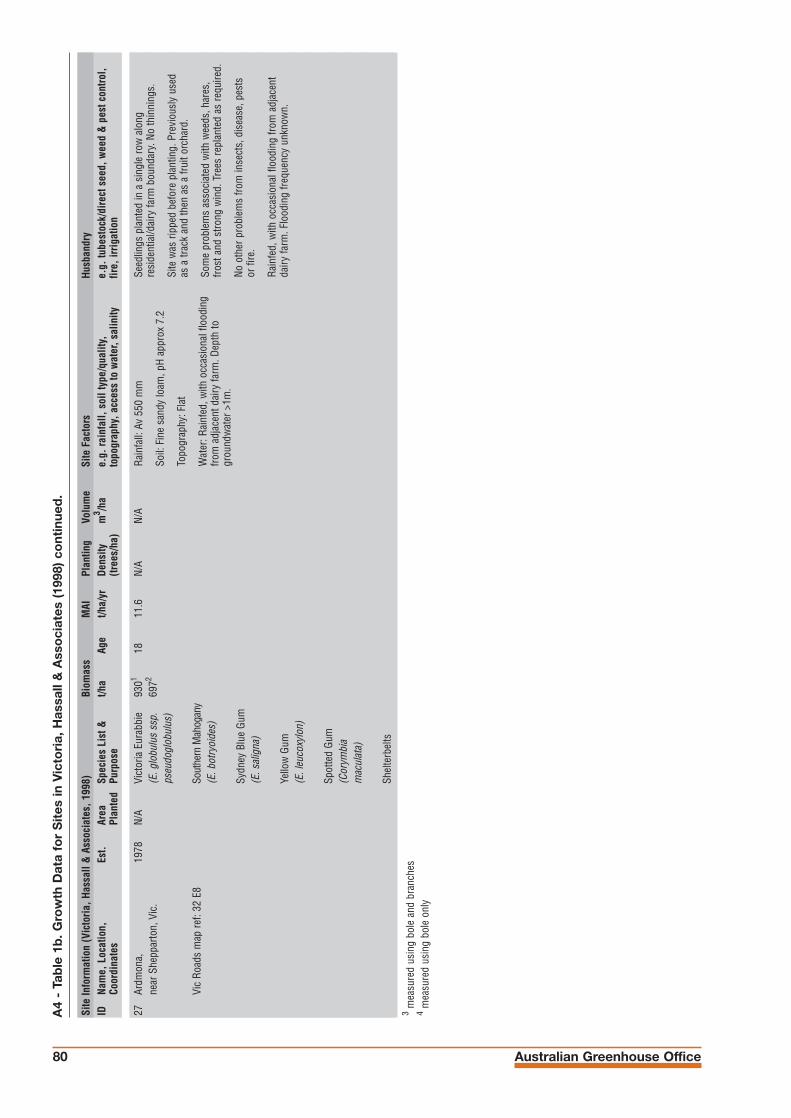
Australian Greenhouse Office80
27Ar
dmon
a,19
78N/
AVi
ctor
ia E
urab
bie
9301
1811
.6N/
AN/
Ane
ar S
hepp
arto
n, V
ic.
(E. g
lobu
lus
ssp.
69
72
pseu
dogl
obul
us)
Vic
Road
s m
ap re
f: 32
E8
Sout
hern
Mah
ogan
y(E
. bot
ryoi
des)
Sydn
ey B
lue
Gum
(E. s
alig
na)
Yello
w G
um
(E. l
euco
xylo
n)
Spot
ted
Gum
(C
orym
bia
mac
ulat
a)
Shel
terb
elts
Rain
fall:
Av
550
mm
Soil:
Fin
e sa
ndy
loam
, pH
appr
ox 7
.2
Topo
grap
hy: F
lat
Wat
er: R
ainf
ed, w
ith o
ccas
iona
l flo
odin
gfro
m a
djac
ent d
airy
farm
. Dep
th to
grou
ndw
ater
>1m
.
Seed
lings
pla
nted
in a
sin
gle
row
alo
ngre
side
ntia
l/dai
ry fa
rm b
ound
ary.
No
thin
ning
s.
Site
was
ripp
ed b
efor
e pl
antin
g. P
revi
ousl
y us
edas
a tr
ack
and
then
as
a fru
it or
char
d.
Som
e pr
oble
ms
asso
ciat
ed w
ith w
eeds
, har
es,
frost
and
stro
ng w
ind.
Tre
es re
plan
ted
as re
quire
d.
No o
ther
pro
blem
s fro
m in
sect
s, d
isea
se, p
ests
orfir
e.
Rain
fed,
with
occ
asio
nal f
lood
ing
from
adj
acen
tda
iry fa
rm. F
lood
ing
frequ
ency
unk
now
n.
Site
Info
rmat
ion
(Vic
toria
, Has
sall
& A
ssoc
iate
s, 1
998)
Biom
ass
MAI
Plan
ting
Volu
me
Site
Fac
tors
Husb
andr
yID
Na
me,
Loc
atio
n,
Est.
Area
Sp
ecie
s Li
st &
t/ha
Age
t/ha/
yrDe
nsity
m
3 /ha
e.g.
rain
fall,
soi
l typ
e/qu
ality
,e.
g. tu
best
ock/
dire
ct s
eed,
wee
d &
pes
t con
trol,
Coor
dina
tes
Plan
ted
Purp
ose
(tree
s/ha
)to
pogr
aphy
, acc
ess
to w
ater
, sal
inity
fire,
irrig
atio
n
3m
easu
red
usin
g bo
le a
nd b
ranc
hes
4m
easu
red
usin
g bo
le o
nly
A4
- Ta
ble
1b
. Gro
wth
Dat
a fo
r S
ites
in V
icto
ria,
Has
sall
& A
sso
ciat
es (
1998
) co
ntin
ued
.

National Carbon Accounting System Technical Report 81
1W
ongo
n Hi
lls19
653.
5 ha
Dwar
f Sug
ar G
um76
132
.52.
415
0N/
A(E
.cla
doca
lyx
572
var.
nana
)
Amen
ity
2W
ongo
n Hi
lls19
653.
5 ha
Suga
r Gum
16
0132
.54.
911
0N/
A(E
. cla
doca
lyx)
1202
Amen
ity
3W
ongo
n Hi
lls19
518
haSa
lt Ri
ver G
um73
146
.51.
620
0N/
A(E
. sar
gent
ii)55
2
Eros
ion
cont
rol,
wat
erta
ble/
dryl
and
salin
ity c
ontro
l
4Ej
andi
ng W
est
1984
20 h
aDw
arf S
ugar
Gum
681
13.5
285
N/A
(E. c
lado
caly
x 51
2
var.
nana
)
Coas
tal M
ort
(E. p
laty
pus
var.
hete
roph
ylla
)
Eros
ion
cont
rol,
wat
erta
ble/
dryl
and
salin
ity c
ontro
l, w
indb
reak
Site
Info
rmat
ion
(Wes
tern
Aus
tralia
, Has
sall
& A
ssoc
iate
s, 1
999b
)Bi
omas
sM
AIPl
antin
gVo
lum
eSi
te F
acto
rsHu
sban
dry
ID
Nam
e, L
ocat
ion,
Es
t.Ar
ea
Spec
ies
List
&t/h
aAg
et/h
a/yr
Dens
ity
m3 /h
ae.
g. ra
infa
ll, s
oil t
ype/
qual
ity,
e.g.
tube
stoc
k/di
rect
see
d, w
eed
& p
est c
ontro
l,Co
ordi
nate
sPl
ante
dPu
rpos
e(tr
ees/
ha)
topo
grap
hy, a
cces
s to
wat
er, s
alin
ityfir
e, ir
rigat
ion
A4
- Ta
ble
1c.
Gro
wth
Dat
a fo
r S
ites
in W
este
rn A
ustr
alia
, Has
sall
& A
sso
ciat
es (
1999
b)
Rain
fall:
Av
392
mm
Soil:
Yel
low
/bro
wn
sand
ove
r dee
p lo
amy
sand
, pH
appr
ox 4
.8-5
.2 (C
aCl2
)
Topo
grap
hy: G
ently
und
ulat
ing
Wat
er: R
ainf
ed o
nly,
dep
th to
grou
ndw
ater
>1m
Aspe
ct: N
E.
Site
pre
para
tion
unkn
own.
Pre
viou
sly
crop
ping
/gra
zing.
Tube
stoc
k pl
ante
d in
row
s
No th
inni
ngs
and
no re
plan
ting.
Som
e sp
ecie
s ha
ve s
uffe
red
from
com
petit
ion
from
mor
e vi
goro
us s
peci
es. N
o ot
her p
robl
ems
asso
ciat
ed w
ith w
eeds
/dis
ease
/pes
ts, d
roug
htor
fire.
Rain
fed
only.
Rain
fall:
Av
392
mm
Soil:
Bla
ck c
laye
y sa
nd o
ver b
row
n sa
ndy
loam
, pH
appr
ox 5
.0 (C
aCl2
)
Topo
grap
hy: F
lat
Wat
er: R
ainf
ed p
lus
poss
ible
acc
ess
togr
ound
wat
er, d
epth
to g
roun
dwat
erap
prox
20
cm
Aspe
ct: N
/A.
Site
pre
para
tion
unkn
own.
Prio
r lan
dus
eun
know
n.
Tube
stoc
k pl
ante
d in
row
s al
ong
cont
ours
.
No th
inni
ngs,
but
site
repl
ante
d to
repl
ace
deat
hsan
d in
crea
se d
ensi
ty.
Inci
denc
e of
wee
ds/d
isea
se/p
ests
, dro
ught
or
fire
unkn
own.
Rain
fed
plus
acc
ess
to s
hallo
w g
roun
dwat
er.
Rain
fall:
Av
311
mm
Soil:
San
d ov
er y
ello
w b
row
n cl
ayey
sand
, non
-sal
ine,
pH
appr
ox 4
.5
Topo
grap
hy: G
entle
slo
pe
Wat
er: R
ainf
ed o
nly,
dep
th to
grou
ndw
ater
app
rox
10-1
2m
Aspe
ct: W
.
Site
ripp
ed p
rior t
o pl
antin
g. P
revi
ousl
y us
ed fo
rcr
oppi
ng/g
razin
g.
Tube
stoc
k pl
ante
d in
row
s ac
ross
con
tour
s.
No th
inni
ngs.
Som
e in
itial
loss
of t
rees
due
todr
ough
t and
win
d da
mag
e, b
ut n
one
sinc
e.
Inci
denc
e of
wee
ds/d
isea
se/p
ests
, dro
ught
or
fire
unkn
own.
Rain
fed
only.
See
abov
eSe
e ab
ove

Australian Greenhouse Office82
Site
Info
rmat
ion
(Wes
tern
Aus
tralia
, Has
sall
& A
ssoc
iate
s, 1
999b
)Bi
omas
sM
AIPl
antin
gVo
lum
eSi
te F
acto
rsHu
sban
dry
ID
Nam
e, L
ocat
ion,
Es
t.Ar
ea
Spec
ies
List
&t/h
aAg
et/h
a/yr
Dens
ity
m3 /h
ae.
g. ra
infa
ll, s
oil t
ype/
qual
ity,
e.g.
tube
stoc
k/di
rect
see
d, w
eed
& p
est c
ontro
l,Co
ordi
nate
sPl
ante
dPu
rpos
e(tr
ees/
ha)
topo
grap
hy, a
cces
s to
wat
er, s
alin
ityfir
e, ir
rigat
ion
5Ej
andi
ng19
852
haSa
lt Ri
ver G
um10
112
.550
0N/
A(E
. sar
gent
ii)72
Eros
ion
cont
rol,
wat
erta
ble/
dryl
and
salin
ity c
ontro
l
6Tr
ayni
ng19
871
haRi
ver R
ed G
um45
110
.545
0-50
0N/
A(E
. cam
aldu
lens
is)
342
Eros
ion
cont
rol,
wat
erta
ble/
dryl
and
salin
ity c
ontro
l
7Tr
ayni
ng19
871
haSe
e ab
ove
7.31
10.5
450-
500
N/A
5.42
8Tr
ayni
ng19
871
haSa
lt Ri
ver G
um28
110
.545
0-50
0N/
A(E
. sar
gent
ii)21
2
Eros
ion
cont
rol,
wat
erta
ble/
dryl
and
salin
ity c
ontro
l
9Tr
ayni
ng19
871
haSe
e ab
ove
3.91
10.5
450-
500
N/A
3.02
Rain
fall:
Av
311
mm
Soil:
yel
low
bro
wn
sand
ove
r lig
ht g
rey
sand
y cl
ay lo
am, m
oder
ate
salin
ity, p
Hap
prox
5.0
Topo
grap
hy: u
nkno
wn
Wat
er: R
ainf
ed p
lus
poss
ible
acc
ess
togr
ound
wat
er, d
epth
to g
roun
dwat
erap
prox
20
cm
Aspe
ct: N
/A.
Site
ripp
ed a
nd s
pray
ed p
rior t
o pl
antin
g.Pr
evio
usly
use
d fo
r cro
ppin
g/gr
azin
g.
Seed
lings
pla
nted
in ro
ws
para
llel t
o a
bulld
ozed
drai
n lin
e us
ing
a tre
e pl
ante
r.
No th
inni
ngs.
Som
e re
cent
dea
ths
due
to d
roug
ht.
No re
plan
ting.
No d
amag
e fro
m w
eeds
/dis
ease
/pes
ts o
r fire
.
Rain
fed
only,
plu
s ac
cess
to s
hallo
w g
roun
dwat
er.
Rain
fall:
Av
323
mm
Soil:
Yel
low
bro
wn
sand
ove
r brig
htye
llow
bro
wn
sand
y lo
am, p
H 6.
1
Topo
grap
hy: M
idsl
ope,
ver
y ge
ntle
slo
pe
Wat
er: R
ainf
ed o
nly,
dep
th to
grou
ndw
ater
app
rox
30 c
m
Aspe
ct: N
NE.
Site
ripp
ed a
nd s
pray
ed p
rior t
o pl
antin
g.Pr
evio
usly
use
d fo
r cro
ppin
g.
Seed
lings
pla
nted
in c
onto
ured
row
s us
ing
atre
epl
ante
r.
No th
inni
ngs.
Som
e re
cent
dea
ths
due
to d
roug
ht.
No re
plan
ting.
No d
amag
e fro
m w
eeds
/dis
ease
/pes
ts o
r fire
.
Rain
fed
only.
See
abov
e ex
cept
:
Wat
er: R
ainf
ed o
nly,
dep
th to
grou
ndw
ater
>1.
5m.
See
abov
e
See
abov
e ex
cept
:
pH 5
.1
Aspe
ct: S
SW.
See
abov
e ex
cept
:
Som
e de
aths
due
to b
orer
s in
the
drie
r are
as.
See
abov
eSe
e ab
ove
A4
- Ta
ble
1c.
Gro
wth
Dat
a fo
r S
ites
in W
este
rn A
ustr
alia
, Has
sall
& A
sso
ciat
es (
1999
b)
cont
inue
d.

National Carbon Accounting System Technical Report 83
Site
Info
rmat
ion
(Wes
tern
Aus
tralia
, Has
sall
& A
ssoc
iate
s, 1
999b
)Bi
omas
sM
AIPl
antin
gVo
lum
eSi
te F
acto
rsHu
sban
dry
ID
Nam
e, L
ocat
ion,
Es
t.Ar
ea
Spec
ies
List
&t/h
aAg
et/h
a/yr
Dens
ity
m3 /h
ae.
g. ra
infa
ll, s
oil t
ype/
qual
ity,
e.g.
tube
stoc
k/di
rect
see
d, w
eed
& p
est c
ontro
l,Co
ordi
nate
sPl
ante
dPu
rpos
e(tr
ees/
ha)
topo
grap
hy, a
cces
s to
wat
er, s
alin
ityfir
e, ir
rigat
ion
10Be
ncub
bin
1982
N/A
Rive
r Red
Gum
161
15.5
500
N/A
(E. c
amal
dule
nsis
)12
2
Win
dbre
ak
11Be
acon
1986
0.25
ha
Rive
r Red
Gum
111
11.5
200
N/A
(E. c
amal
dule
nsis
)82
Shad
e an
d sh
elte
r
12M
urki
nbud
in19
861.
5 ha
York
Gum
(I)
181
11.5
250
N/A
132
Stric
klan
d’s
Gum
(E. s
trick
land
ii)
Shea
th’s
Gum
(E. s
heat
hian
a)
Eros
ion
cont
rol,
wat
erta
ble/
dryl
and
salin
ity c
ontro
l
Rain
fall:
Av
322
mm
Soil:
Dee
p ye
llow
wod
jil s
ands
,pH
4.5
(H20
)
Topo
grap
hy: H
igh
up o
n a
gent
lysl
opin
ghi
llsid
e
Wat
er: R
ainf
ed o
nly,
dep
th to
grou
ndw
ater
unk
now
n bu
t dee
p
Aspe
ct: W
.
Site
ripp
ed a
nd s
pray
ed p
rior t
o pl
antin
g.Pr
evio
usly
use
d fo
r cro
ppin
g/gr
azin
g.
Seed
lings
pla
nted
in ro
ws.
Thi
nnin
gshi
stor
yun
know
n.
Initi
al d
eath
s du
e to
rabb
its. T
reat
ed b
y ba
iting
and
prot
ectiv
e ne
tting
. See
dlin
gs re
plan
ted.
Som
ere
cent
dea
ths
due
to d
roug
ht a
nd a
ssoc
iate
d bo
rer
activ
ity. N
o tre
atm
ent.
Rain
fed
only.
Rain
fall:
Av
314
mm
Soil:
Red
dish
bro
wn
sand
y lo
am, l
owsa
linity
, pH
7.6-
7.8
(H20
)
Topo
grap
hy: F
lat
Wat
er: R
ainf
ed p
lus
acce
ss to
grou
ndw
ater
. Dep
th to
gro
undw
ater
appr
ox 1
.5m
, sal
inity
600
0 m
S/m
Aspe
ct: N
/A.
Site
pre
para
tion
hist
ory
unkn
own.
Pre
viou
sly
used
for c
ropp
ing/
graz
ing.
Seed
lings
pla
nted
in ro
ws
by h
and.
Thi
nnin
gshi
stor
y un
know
n.
The
only
site
diff
icul
ty a
ppea
rs to
be
reas
onab
lysh
allo
w a
nd s
alin
e gr
ound
wat
er.
Rain
fed
plus
acc
ess
to g
roun
dwat
er.
Rain
fall:
Av
285
mm
Soil:
Bro
wn
sand
y lo
am, o
ver b
edro
ck,
salt
scal
ds in
par
ts, m
oder
atel
y ac
id.
Topo
grap
hy: V
ery
gent
le m
idsl
ope
Wat
er: R
ainf
ed p
lus
pote
ntia
l acc
ess
togr
ound
wat
er s
eep.
Dep
th to
grou
ndw
ater
unkn
own.
Aspe
ct: S
.
Site
ripp
ed b
ut n
ot s
pray
ed. P
revi
ousl
y us
ed fo
rcr
oppi
ng/g
razin
g.
Seed
lings
pla
nted
in 5
con
tour
ed ro
ws
adja
cent
salt
scal
d us
ing
a tre
e pl
ante
r. Th
inni
ngs
hist
ory
unkn
own.
No re
porte
d pr
oble
ms
with
pes
ts/w
eeds
/dis
ease
,fir
e or
dro
ught
.
Rain
fed,
plu
s po
tent
ial a
cces
s to
gro
undw
ater

Australian Greenhouse Office84
13Be
lka
East
1988
2 ha
Rive
r Red
Gum
561
9.5
N/A
N/A
(E. c
amal
dule
nsis
)42
2
Red
Ironb
ark
(E. s
ider
oxyl
on)
Eros
ion
cont
rol,
wat
erta
ble/
dryl
and
salin
ity c
ontro
l,am
enity
14Be
lka
East
1988
2 ha
See
abov
e,
301
9.5
N/A
N/A
exce
pt o
nly
222
Red
Ironb
ark
(E. s
ider
oxyl
on)
15Ba
kers
Hill
1978
N/A
Rive
r Red
Gum
381
19.5
Orig
inal
lyN/
A(la
rger
(E. c
amal
dule
nsis
)28
255
0, n
ow
than
muc
h th
ose
Eros
ion
cont
rol,
low
erbe
low
)w
ater
tabl
e/dr
ylan
dsa
linity
con
trol,
expe
rimen
t
16Ba
kers
Hill
1977
1 ha
See
abov
e46
120
.565
0N/
A35
2
17Ba
kers
Hill
1984
1.5
haSe
e ab
ove
301
13.5
260
N/A
222
Site
Info
rmat
ion
(Wes
tern
Aus
tralia
, Has
sall
& A
ssoc
iate
s, 1
999b
)Bi
omas
sM
AIPl
antin
gVo
lum
eSi
te F
acto
rsHu
sban
dry
ID
Nam
e, L
ocat
ion,
Es
t.Ar
ea
Spec
ies
List
&t/h
aAg
et/h
a/yr
Dens
ity
m3 /h
ae.
g. ra
infa
ll, s
oil t
ype/
qual
ity,
e.g.
tube
stoc
k/di
rect
see
d, w
eed
& p
est c
ontro
l,Co
ordi
nate
sPl
ante
dPu
rpos
e(tr
ees/
ha)
topo
grap
hy, a
cces
s to
wat
er, s
alin
ityfir
e, ir
rigat
ion
Rain
fall:
Av
332
mm
Soil:
San
d ov
er b
right
yel
low
ish
brow
nsa
ndy
loam
, pH
4.2
Topo
grap
hy: M
idsl
ope
Wat
er: R
ainf
ed p
lus
pote
ntia
l acc
ess
togr
ound
wat
er s
eep,
dep
th to
grou
ndw
ater
>5m
Aspe
ct: N
E.
Site
ripp
ed a
nd s
pray
ed th
e ye
ar b
efor
e.Pr
evio
usly
use
d fo
r cro
ppin
g/gr
azin
g.
Seed
lings
pla
nted
in c
onto
ured
row
s pe
rpen
dicu
lar
from
see
p us
ing
a tre
e pl
ante
r. No
thin
ning
s.
No re
porte
d pr
oble
ms
with
pes
ts/w
eeds
/dis
ease
,fir
e or
dro
ught
.
Rain
fed,
plu
s po
tent
ial a
cces
s to
gro
undw
ater
.
See
abov
e ex
cept
:
No a
cces
s to
gro
undw
ater
see
p,gr
eate
rdep
th.
See
abov
e ex
cept
:
Low
er g
row
th ra
tes
asso
ciat
ed w
ith d
roug
htin
g.
Rain
fall:
Av
593
mm
Soil:
Bro
wni
sh b
lack
gra
velly
san
d ov
ergr
avel
ly y
ello
w o
rang
e sa
nd,
pHun
know
n.
Topo
grap
hy: V
ery
gent
ly s
lopi
nglo
whi
llsid
e.
Wat
er: R
ainf
ed, d
epth
togr
ound
wat
er>2
m
Aspe
ct: U
nkno
wn.
Site
pre
para
tion
unkn
own.
Pre
viou
sly
used
forg
razin
g.
Tree
s pl
ante
d in
row
s. T
hinn
ings
occ
urre
d se
vera
lye
ars
ago.
Hist
ory
of p
robl
ems
with
pes
ts/w
eeds
/dis
ease
, fire
or d
roug
ht u
nkno
wn.
Rain
fed
only.
See
abov
e ex
cept
:
Soil:
Dar
k br
own
grav
elly
loam
y sa
ndov
er a
gra
velly
cla
yey
sand
.
See
abov
e, e
xcep
t:
No th
inni
ngs.
See
abov
e ex
cept
:
Soil:
Dar
k br
own
loam
y sa
nd o
ver
yello
wis
h br
own
light
cla
y w
ith m
ottle
s.Ad
jace
nt s
alin
e ar
eas.
Wat
er: R
ainf
ed, d
epth
togr
ound
wat
er<2
m.
See
abov
e
A4
- Ta
ble
1c.
Gro
wth
Dat
a fo
r S
ites
in W
este
rn A
ustr
alia
, Has
sall
& A
sso
ciat
es (
1999
b)
cont
inue
d.
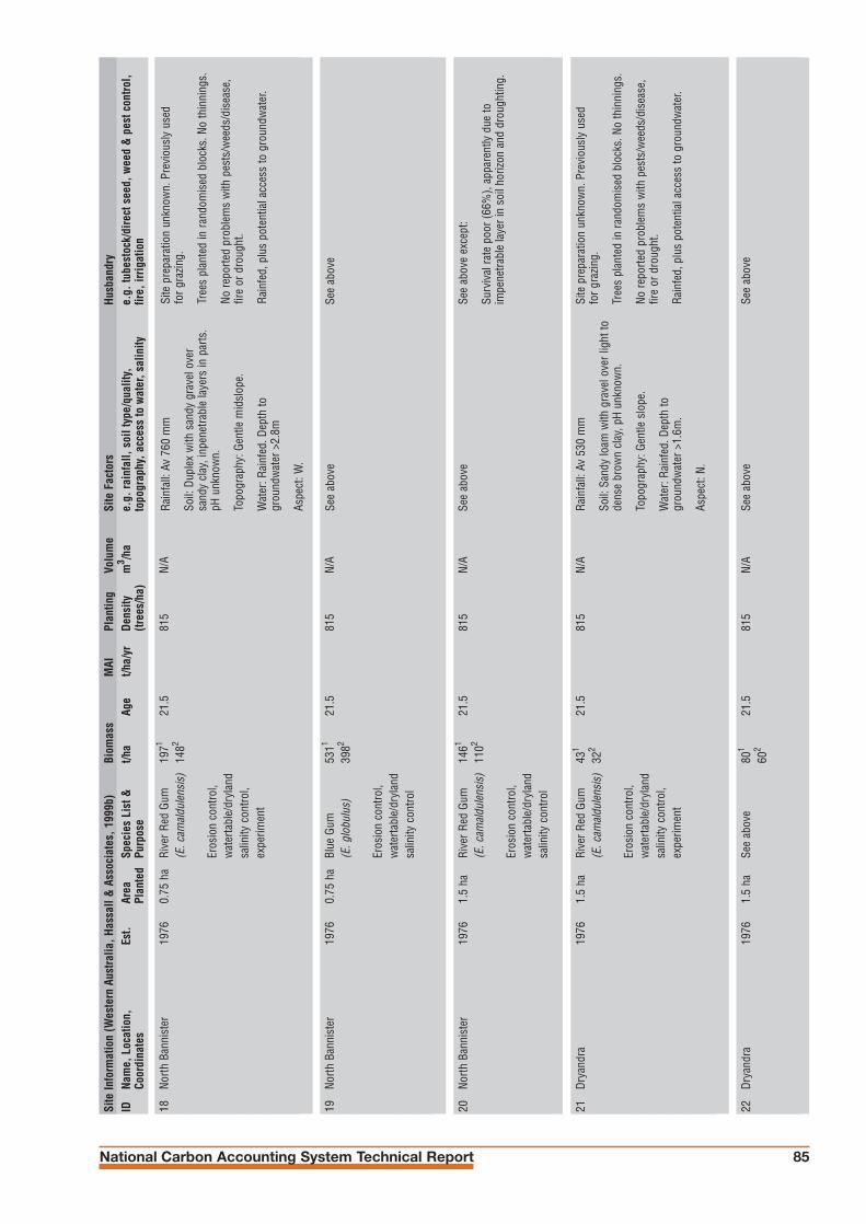
National Carbon Accounting System Technical Report 85
18No
rth B
anni
ster
1976
0.75
ha
Rive
r Red
Gum
1971
21.5
815
N/A
(E. c
amal
dule
nsis
)14
82
Eros
ion
cont
rol,
wat
erta
ble/
dryl
and
salin
ity c
ontro
l, ex
perim
ent
19No
rth B
anni
ster
1976
0.75
ha
Blue
Gum
5311
21.5
815
N/A
(E. g
lobu
lus)
3982
Eros
ion
cont
rol,
wat
erta
ble/
dryl
and
salin
ity c
ontro
l
20No
rth B
anni
ster
1976
1.5
haRi
ver R
ed G
um14
6121
.581
5N/
A(E
. cam
aldu
lens
is)
1102
Eros
ion
cont
rol,
wat
erta
ble/
dryl
and
salin
ity c
ontro
l
21Dr
yand
ra19
761.
5 ha
Rive
r Red
Gum
431
21.5
815
N/A
(E. c
amal
dule
nsis
)32
2
Eros
ion
cont
rol,
wat
erta
ble/
dryl
and
salin
ity c
ontro
l,ex
perim
ent
22Dr
yand
ra19
761.
5 ha
See
abov
e80
121
.581
5N/
A60
2
Rain
fall:
Av
760
mm
Soil:
Dup
lex
with
san
dy g
rave
l ove
rsa
ndy
clay
, inp
enet
rabl
e la
yers
in p
arts
.pH
unk
now
n.
Topo
grap
hy: G
entle
mid
slop
e.
Wat
er: R
ainf
ed. D
epth
togr
ound
wat
er>2
.8m
Aspe
ct: W
.
Site
pre
para
tion
unkn
own.
Pre
viou
sly
used
forg
razin
g.
Tree
s pl
ante
d in
rand
omis
ed b
lock
s. N
o th
inni
ngs.
No re
porte
d pr
oble
ms
with
pes
ts/w
eeds
/dis
ease
,fir
e or
dro
ught
.
Rain
fed,
plu
s po
tent
ial a
cces
s to
gro
undw
ater
.
See
abov
eSe
e ab
ove
Site
Info
rmat
ion
(Wes
tern
Aus
tralia
, Has
sall
& A
ssoc
iate
s, 1
999b
)Bi
omas
sM
AIPl
antin
gVo
lum
eSi
te F
acto
rsHu
sban
dry
ID
Nam
e, L
ocat
ion,
Es
t.Ar
ea
Spec
ies
List
&t/h
aAg
et/h
a/yr
Dens
ity
m3 /h
ae.
g. ra
infa
ll, s
oil t
ype/
qual
ity,
e.g.
tube
stoc
k/di
rect
see
d, w
eed
& p
est c
ontro
l,Co
ordi
nate
sPl
ante
dPu
rpos
e(tr
ees/
ha)
topo
grap
hy, a
cces
s to
wat
er, s
alin
ityfir
e, ir
rigat
ion
See
abov
eSe
e ab
ove
exce
pt:
Surv
ival
rate
poo
r (66
%),
appa
rent
ly d
ue to
impe
netra
ble
laye
r in
soil
horiz
on a
nd d
roug
htin
g.
Rain
fall:
Av
530
mm
Soil:
San
dy lo
am w
ith g
rave
l ove
r lig
ht to
dens
e br
own
clay
, pH
unkn
own.
Topo
grap
hy: G
entle
slo
pe.
Wat
er: R
ainf
ed. D
epth
togr
ound
wat
er>1
.6m
.
Aspe
ct: N
.
Site
pre
para
tion
unkn
own.
Pre
viou
sly
used
forg
razin
g.
Tree
s pl
ante
d in
rand
omis
ed b
lock
s. N
o th
inni
ngs.
No re
porte
d pr
oble
ms
with
pes
ts/w
eeds
/dis
ease
,fir
e or
dro
ught
.
Rain
fed,
plu
s po
tent
ial a
cces
s to
gro
undw
ater
.
See
abov
eSe
e ab
ove

Australian Greenhouse Office86
23Bi
ngha
m R
iver
1976
N/A
Blue
Gum
831
20N/
AN/
A(E
. glo
bulu
s)62
2
Eros
ion
cont
rol,
wat
erta
ble/
dryl
and
salin
ity c
ontro
l
24Bi
ngha
m R
iver
1978
N/A
See
abov
e69
118
N/A
N/A
522
25Bo
wel
ling
1981
N/A
Rive
r Red
Gum
1131
1460
0N/
A(E
. cam
aldu
lens
is)
852
Eros
ion
cont
rol,
wat
erta
ble/
dryl
and
salin
ity c
ontro
l,w
ood
prod
ucts
26Co
rder
ing
1984
N/A
Blue
Gum
1211
1237
5N/
A(E
. glo
bulu
s)91
2
Eros
ion
cont
rol,
wat
erta
ble/
dryl
and
salin
ity c
ontro
l,w
ood
prod
ucts
27Co
rder
ing
1984
N/A
Rive
r Red
Gum
361
1232
5N/
A(E
. cam
aldu
lens
is)
272
Rain
fall:
Av
713
mm
Soil:
San
d ov
er s
andy
cla
y, p
Hun
know
n.
Topo
grap
hy: G
entle
slo
pe.
Wat
er: R
ainf
ed. D
epth
togr
ound
wat
erun
know
n.
Site
pre
para
tion
unkn
own.
Pre
viou
sly
used
for
mix
ed fa
rmin
g.
Esta
blis
hmen
t and
man
agem
ent r
egim
e un
know
n.
See
abov
eSe
e ab
ove
Rain
fall:
Av
692
mm
Soil:
Hea
vy c
lay,
mod
erat
ely
salin
e(E
C14
0m S
/m),
pH u
nkno
wn.
Topo
grap
hy: F
lat.
Wat
er: R
ainf
ed, p
lus
poss
ible
acc
ess
togr
ound
wat
er. D
epth
to g
roun
dwat
er<1
.5m
. Wat
er ta
ble
salin
ity 2
000
mS/
m.
Site
pre
para
tion
unkn
own.
Pre
viou
sly
used
forg
razin
g.
Tree
s pl
ante
d in
mou
nded
row
s. T
hinn
ings
hist
ory
unkn
own.
No re
porte
d pr
oble
ms
with
pes
ts/w
eeds
/dis
ease
,fir
e or
dro
ught
.
Rain
fed,
plu
s po
tent
ial a
cces
s to
gro
undw
ater
.
Rain
fall:
Av
621
mm
Soil:
N/A
Topo
grap
hy: V
ery
gent
le s
lope
to fl
at.
Wat
er: R
ainf
ed. D
epth
togr
ound
wat
erun
know
n.
Site
pre
para
tion
unkn
own.
Pre
viou
sly
used
forg
razin
g.
Tree
s pl
ante
d in
row
s. T
hinn
ings
his
tory
unk
now
n.
No re
porte
d pr
oble
ms
with
pes
ts/w
eeds
/dis
ease
,fir
e or
dro
ught
.
Rain
fed.
See
abov
eSe
e ab
ove
exce
pt:
Tree
s pl
ante
d on
a s
alt s
cald
and
bar
ley
gras
s si
te.
Site
Info
rmat
ion
(Wes
tern
Aus
tralia
, Has
sall
& A
ssoc
iate
s, 1
999b
)Bi
omas
sM
AIPl
antin
gVo
lum
eSi
te F
acto
rsHu
sban
dry
ID
Nam
e, L
ocat
ion,
Es
t.Ar
ea
Spec
ies
List
&t/h
aAg
et/h
a/yr
Dens
ity
m3 /h
ae.
g. ra
infa
ll, s
oil t
ype/
qual
ity,
e.g.
tube
stoc
k/di
rect
see
d, w
eed
& p
est c
ontro
l,Co
ordi
nate
sPl
ante
dPu
rpos
e(tr
ees/
ha)
topo
grap
hy, a
cces
s to
wat
er, s
alin
ityfir
e, ir
rigat
ion
A4
- Ta
ble
1c.
Gro
wth
Dat
a fo
r S
ites
in W
este
rn A
ustr
alia
, Has
sall
& A
sso
ciat
es (
1999
b)
cont
inue
d.

National Carbon Accounting System Technical Report 87
28Di
nnin
up19
83<
1 ha
Blue
Gum
831
14.5
1,10
0N/
A(E
. glo
bulu
s)62
2
Eros
ion
cont
rol,
wat
erta
ble/
dryl
and
salin
ity c
ontro
l,w
ind
brea
k
29Di
nnin
up19
84<
1 ha
Rive
r Red
Gum
771
13.5
1,10
0N/
A(E
. cam
aldu
lens
is)
582
30Di
nnin
up19
83<
1 ha
Blue
Gum
1461
14.5
900
N/A
(E. g
lobu
lus)
1092
31M
ayan
up19
875
haRi
ver R
ed G
um76
18.
550
0N/
A(E
. cam
aldu
lens
is)
572
Eros
ion
cont
rol,
wat
erta
ble/
dryl
and
salin
ity c
ontro
l,am
enity
See
abov
eSe
e ab
ove
exce
pt:
No d
eath
s as
soci
ated
with
dro
ught
ing.
See
abov
e ex
cept
:
Soil:
Gre
y sa
nd o
ver y
ello
w b
row
nlo
amy
sand
.
See
abov
e
Rain
fall:
Av
601
mm
Soil:
Bla
ck lo
am o
ver s
andy
cla
y lo
am,
pH u
nkno
wn.
Topo
grap
hy: G
entle
mid
slop
e.
Wat
er: R
ainf
ed. D
epth
to g
roun
dwat
er>2
m a
lthou
gh it
is w
et in
win
ter.
Aspe
ct: E
.
Site
ripp
ed a
nd s
pray
ed b
ut n
ot m
ound
ed p
rior t
opl
antin
g. P
revi
ousl
y us
ed fo
r gra
zing.
Seed
lings
han
d pl
ante
d in
irre
glua
rly s
pace
d ro
ws.
Thin
ning
s hi
stor
y un
know
n.
No re
porte
d pr
oble
ms
with
wee
ds/d
isea
se o
r fire
.So
me
initi
al d
eath
s fro
m k
anga
roos
and
som
ere
cent
ext
ensi
ve d
eath
s du
e to
dro
ught
ing.
Rain
fed.
Site
Info
rmat
ion
(Wes
tern
Aus
tralia
, Has
sall
& A
ssoc
iate
s, 1
999b
)Bi
omas
sM
AIPl
antin
gVo
lum
eSi
te F
acto
rsHu
sban
dry
ID
Nam
e, L
ocat
ion,
Es
t.Ar
ea
Spec
ies
List
&t/h
aAg
et/h
a/yr
Dens
ity
m3 /h
ae.
g. ra
infa
ll, s
oil t
ype/
qual
ity,
e.g.
tube
stoc
k/di
rect
see
d, w
eed
& p
est c
ontro
l,Co
ordi
nate
sPl
ante
dPu
rpos
e(tr
ees/
ha)
topo
grap
hy, a
cces
s to
wat
er, s
alin
ityfir
e, ir
rigat
ion
Rain
fall:
Av
668
mm
Soil:
Sha
llow
san
d ov
er c
lay,
mod
erat
ely
salin
e (E
C 50
-140
mS/
m),
pH u
nkno
wn.
Topo
grap
hy: G
entle
slo
pe to
flat
.
Wat
er: R
ainf
ed. S
hallo
w, d
epth
unk
now
n,sa
line
(2,2
00m
S/m
)
Aspe
ct: N
.
Site
ripp
ed a
nd m
ound
ed p
rior t
o pl
antin
g.Pr
evio
usly
use
unk
now
n.
Thin
ning
s hi
stor
y un
know
n.
No re
porte
d pr
oble
ms
with
pes
ts/w
eeds
/dis
ease
,dr
ough
t or f
ire.
Rain
fed,
plu
s ac
cess
to g
roud
wat
er.
5m
easu
red
usin
g bo
le a
nd b
ranc
hes
6m
easu
red
usin
g bo
le o
nly

Australian Greenhouse Office88
1RT
123C
, Mt.
Lofty
Ran
ges
1988
N/A
E. g
lobu
lus
3N/
AN/
A4
Rain
fall:
Av
926
mm
Prev
ious
ly p
lant
ed w
ith P
inus
radi
ata.
Sout
hern
Blu
e Gu
mLa
t/lon
g: 3
453,
138
49So
il: L
oam
ove
r med
ium
cla
y, d
epth
to
clay
30
cm
Topo
grap
hy: 2
0% s
lope
.
See
abov
e5
42
See
abov
e7
108
See
abov
e9
200
See
abov
e11
32
See
abov
eN/
AE.
nite
ns3
N/A
N/A
5Sh
inin
g Gu
m
See
abov
e5
65
See
abov
e7
151
See
abov
e9
268
See
abov
e11
390
See
abov
eN/
AE.
vim
inal
isM
anna
Gum
3N/
AN/
A1
See
abov
e5
32
See
abov
e7
89
See
abov
e9
173
See
abov
e11
288
See
abov
eN/
AE.
bot
ryoi
des
3N/
AN/
A4
Sout
hern
Mah
ogan
y
See
abov
e5
37
See
abov
e7
91
A4
- Ta
ble
2a.
Gro
wth
Dat
a fo
r S
ites
in S
out
h A
ustr
alia
, Wo
ng e
t al
.(20
00)
Site
info
rmat
ion
(Sou
th A
ustra
lia, W
ong
et. a
l., 2
000)
Biom
ass
MAI
Plan
ting
Volu
me
Site
Fac
tors
Husb
andr
yID
Na
me,
Loc
atio
n,
Est.
Area
Sp
ecie
s Li
st &
t/ha
Age
t/ha/
yrDe
nsity
m
3 /ha
e.g.
rain
fall,
soi
l typ
e/qu
ality
,e.
g. tu
best
ock/
dire
ct s
eed,
wee
d &
pes
t con
trol,
Coor
dina
tes
Plan
ted
Purp
ose
(tree
s/ha
)to
pogr
aphy
, acc
ess
to w
ater
, sal
inity
fire,
irrig
atio
n
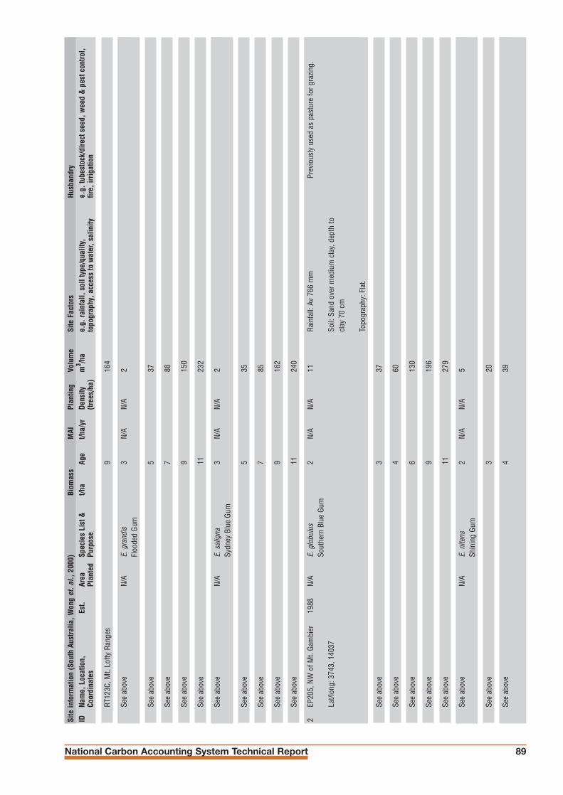
National Carbon Accounting System Technical Report 89
Site
info
rmat
ion
(Sou
th A
ustra
lia, W
ong
et. a
l., 2
000)
Biom
ass
MAI
Plan
ting
Volu
me
Site
Fac
tors
Husb
andr
yID
Na
me,
Loc
atio
n,
Est.
Area
Sp
ecie
s Li
st &
t/ha
Age
t/ha/
yrDe
nsity
m
3 /ha
e.g.
rain
fall,
soi
l typ
e/qu
ality
,e.
g. tu
best
ock/
dire
ct s
eed,
wee
d &
pes
t con
trol,
Coor
dina
tes
Plan
ted
Purp
ose
(tree
s/ha
)to
pogr
aphy
, acc
ess
to w
ater
, sal
inity
fire,
irrig
atio
n
RT12
3C, M
t. Lo
fty R
ange
s9
164
See
abov
eN/
AE.
gra
ndis
3N/
AN/
A2
Floo
ded
Gum
See
abov
e5
37
See
abov
e7
88
See
abov
e9
150
See
abov
e11
232
See
abov
eN/
AE.
sal
igna
3N/
AN/
A2
Sydn
ey B
lue
Gum
See
abov
e5
35
See
abov
e7
85
See
abov
e9
162
See
abov
e11
240
2EP
205,
NW
of M
t. Ga
mbi
er19
88N/
AE.
glo
bulu
s2
N/A
N/A
11Ra
infa
ll: A
v 76
6 m
mPr
evio
usly
use
d as
pas
ture
for g
razin
g.So
uthe
rn B
lue
Gum
Lat/l
ong:
374
3, 1
4037
Soil:
San
d ov
er m
ediu
m c
lay,
dep
th to
clay
70
cm
Topo
grap
hy: F
lat.
See
abov
e3
37
See
abov
e4
60
See
abov
e6
130
See
abov
e9
196
See
abov
e11
279
See
abov
eN/
AE.
nite
ns2
N/A
N/A
5Sh
inin
g Gu
m
See
abov
e3
20
See
abov
e4
39

Australian Greenhouse Office90
See
abov
e6
93
See
abov
e9
147
See
abov
eN/
AE.
vim
inal
is2
N/A
N/A
4M
anna
Gum
See
abov
e3
20
See
abov
e4
37
See
abov
e6
80
See
abov
e9
123
See
abov
eN/
AE.
bot
ryoi
des
2N/
AN/
A5
Sout
hern
Mah
ogan
y
See
abov
e3
20
See
abov
e4
35
See
abov
e6
92
See
abov
e9
147
3EM
133,
N o
f Mt.
Gam
bier
1991
N/A
E. g
lobu
lus
2N/
AN/
A3
Rain
fall:
Av
745
mm
Prev
ious
ly u
sed
as p
astu
re fo
r gra
zing.
Sout
hern
Blu
e Gu
mLa
t/lon
g: 3
745,
140
47So
il: U
nifo
rm s
andy
pro
file,
dep
th to
clay
200
cm
+
Topo
grap
hy: F
lat.
See
abov
e3
21
See
abov
e4
48
See
abov
e5
69
See
abov
eN/
AE.
sal
igna
Sydn
ey B
lue
Gum
3N/
AN/
A4
See
abov
e4
15
See
abov
e5
24
Site
info
rmat
ion
(Sou
th A
ustra
lia, W
ong
et. a
l., 2
000)
Biom
ass
MAI
Plan
ting
Volu
me
Site
Fac
tors
Husb
andr
yID
Na
me,
Loc
atio
n,
Est.
Area
Sp
ecie
s Li
st &
t/ha
Age
t/ha/
yrDe
nsity
m
3 /ha
e.g.
rain
fall,
soi
l typ
e/qu
ality
,e.
g. tu
best
ock/
dire
ct s
eed,
wee
d &
pes
t con
trol,
Coor
dina
tes
Plan
ted
Purp
ose
(tree
s/ha
)to
pogr
aphy
, acc
ess
to w
ater
, sal
inity
fire,
irrig
atio
n
A4
- Ta
ble
2a.
Gro
wth
Dat
a fo
r S
ites
in S
out
h A
ustr
alia
, Wo
ng e
t al
.(20
00)
cont
inue
d.

National Carbon Accounting System Technical Report 91
See
abov
eN/
AE.
gra
ndis
Floo
ded
Gum
2N/
AN/
A1
EM13
3, N
of M
t. Ga
mbi
er3
13
See
abov
e4
37
See
abov
e5
51
Site
info
rmat
ion
(Sou
th A
ustra
lia, W
ong
et. a
l., 2
000)
Biom
ass
MAI
Plan
ting
Volu
me
Site
Fac
tors
Husb
andr
yID
Na
me,
Loc
atio
n,
Est.
Area
Sp
ecie
s Li
st &
t/ha
Age
t/ha/
yrDe
nsity
m
3 /ha
e.g.
rain
fall,
soi
l typ
e/qu
ality
,e.
g. tu
best
ock/
dire
ct s
eed,
wee
d &
pes
t con
trol,
Coor
dina
tes
Plan
ted
Purp
ose
(tree
s/ha
)to
pogr
aphy
, acc
ess
to w
ater
, sal
inity
fire,
irrig
atio
n

Australian Greenhouse Office92
Site
info
rmat
ion
(Vic
toria
, Won
g et
. al.,
200
0)Bi
omas
sM
AIPl
antin
gVo
lum
eSi
te F
acto
rsHu
sban
dry
ID
Nam
e, L
ocat
ion,
Es
t.Ar
ea
Spec
ies
List
&t/h
aAg
et/h
a/yr
Dens
ity
m3 /h
ae.
g. ra
infa
ll, s
oil t
ype/
qual
ity,
e.g.
tube
stoc
k/di
rect
see
d, w
eed
& p
est c
ontro
l,Co
ordi
nate
sPl
ante
dPu
rpos
e(tr
ees/
ha)
topo
grap
hy, a
cces
s to
wat
er, s
alin
ityfir
e, ir
rigat
ion
1To
star
ee,
1988
N/A
E. g
lobu
lus
2N/
A95
113
near
Lak
es E
ntra
nce,
Vic
.So
uthe
rn B
lue
Gum
Lat/l
ong:
374
7S, 1
4811
E
See
abov
e4
942
74
See
abov
e6
924
157
See
abov
e8
884
262
See
abov
e10
840
334
2To
star
eeE.
nite
ns2
N/A
920
13Sh
inin
g Gu
m
See
abov
e4
916
76
See
abov
e6
900
147
See
abov
e8
860
237
See
abov
e10
832
287
3To
star
eeE.
vim
inal
is2
N/A
980
12M
anna
Gum
See
abov
e4
904
81
See
abov
e6
892
166
See
abov
e8
876
262
See
abov
e10
872
319
4To
star
eeE.
bot
ryoi
des
2N/
A96
48
Sout
hern
Mah
ogan
y
See
abov
e4
960
49
See
abov
e6
952
103
See
abov
e8
936
171
See
abov
e10
888
216
A4
- Ta
ble
2b
. Gro
wth
Dat
a fo
r S
ites
in V
icto
ria,
Wo
ng e
t al
.(20
00)
Rain
fall:
Av
819
mm
Soil:
Loa
my
sand
ove
r lig
ht m
ediu
m c
lay
Topo
grap
hy: 3
-6%
slo
pe.
Smal
l sca
le p
lot (
<1 h
a).
Prev
ious
ly u
sed
for g
razin
g on
impr
oved
pas
ture
with
a h
isto
ry o
f rel
ativ
ely
high
rate
s of
ferti
liser
appl
icat
ion.
Dire
ct s
eedi
ng.

National Carbon Accounting System Technical Report 93
5To
star
eeE.
gra
ndis
2N/
A98
08
Floo
ded
Gum
See
abov
e4
972
45
See
abov
e6
972
93
See
abov
e8
960
161
See
abov
e10
940
215
6To
star
eeE.
sal
igna
2N/
A96
08
Sydn
ey B
lue
Gum
See
abov
e4
948
46
See
abov
e6
948
95
See
abov
e8
928
154
See
abov
e10
N/A
908
195
7W
ayga
ra,
1989
N/A
E. g
lobu
lus
2N/
A93
810
near
Orb
ost,
Vic.
Sout
hern
Blu
e Gu
m
Lat/l
ong:
374
1S, 1
4819
E
See
abov
e4
938
65
See
abov
e6
917
115
See
abov
e8
892
159
See
abov
e10
858
181
8W
ayga
raE.
nite
ns2
695
5Sh
inin
g Gu
m
See
abov
e4
685
41
See
abov
e6
662
70
See
abov
e8
643
87
See
abov
e10
656
114
Site
info
rmat
ion
(Vic
toria
, Won
g et
. al.,
200
0)Bi
omas
sM
AIPl
antin
gVo
lum
eSi
te F
acto
rsHu
sban
dry
ID
Nam
e, L
ocat
ion,
Es
t.Ar
ea
Spec
ies
List
&t/h
aAg
et/h
a/yr
Dens
ity
m3 /h
ae.
g. ra
infa
ll, s
oil t
ype/
qual
ity,
e.g.
tube
stoc
k/di
rect
see
d, w
eed
& p
est c
ontro
l,Co
ordi
nate
sPl
ante
dPu
rpos
e(tr
ees/
ha)
topo
grap
hy, a
cces
s to
wat
er, s
alin
ityfir
e, ir
rigat
ion
Rain
fall:
Av
870
mm
Soil:
Loa
m o
ver l
ight
med
ium
cla
y
Topo
grap
hy: F
lat.
Smal
l sca
le p
lot (
<1 h
a).
Prev
ious
land
use
deg
rade
d na
tive
fore
st s
ever
ely
affe
cted
by
fung
al p
atho
gen
Phyt
opht
hora
cinn
amom
i. Cl
eare
d be
fore
dire
ct s
eedi
ng.
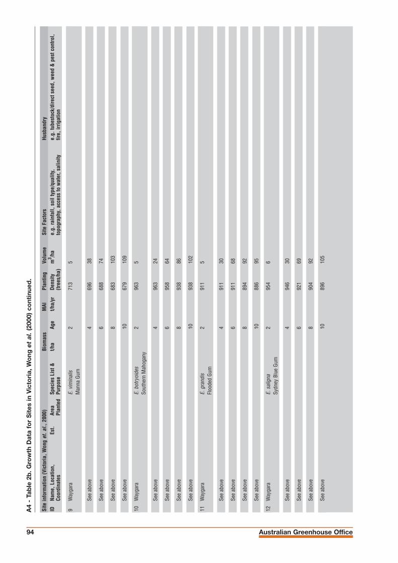
Australian Greenhouse Office94
9W
ayga
raE.
vim
inal
is2
713
5M
anna
Gum
See
abov
e4
696
38
See
abov
e6
688
74
See
abov
e8
683
103
See
abov
e10
679
109
10W
ayga
raE.
bot
ryoi
des
296
35
Sout
hern
Mah
ogan
y
See
abov
e4
963
24
See
abov
e6
958
64
See
abov
e8
938
86
See
abov
e10
938
102
11W
ayga
raE.
gra
ndis
291
15
Floo
ded
Gum
See
abov
e4
911
30
See
abov
e6
911
68
See
abov
e8
894
92
See
abov
e10
886
95
12W
ayga
raE.
sal
igna
295
46
Sydn
ey B
lue
Gum
See
abov
e4
946
30
See
abov
e6
921
69
See
abov
e8
904
92
See
abov
e10
896
105
Site
info
rmat
ion
(Vic
toria
, Won
g et
. al.,
200
0)Bi
omas
sM
AIPl
antin
gVo
lum
eSi
te F
acto
rsHu
sban
dry
ID
Nam
e, L
ocat
ion,
Es
t.Ar
ea
Spec
ies
List
&t/h
aAg
et/h
a/yr
Dens
ity
m3 /h
ae.
g. ra
infa
ll, s
oil t
ype/
qual
ity,
e.g.
tube
stoc
k/di
rect
see
d, w
eed
& p
est c
ontro
l,Co
ordi
nate
sPl
ante
dPu
rpos
e(tr
ees/
ha)
topo
grap
hy, a
cces
s to
wat
er, s
alin
ityfir
e, ir
rigat
ion
A4
- Ta
ble
2b
. Gro
wth
Dat
a fo
r S
ites
in V
icto
ria,
Wo
ng e
t al
.(20
00)
cont
inue
d.
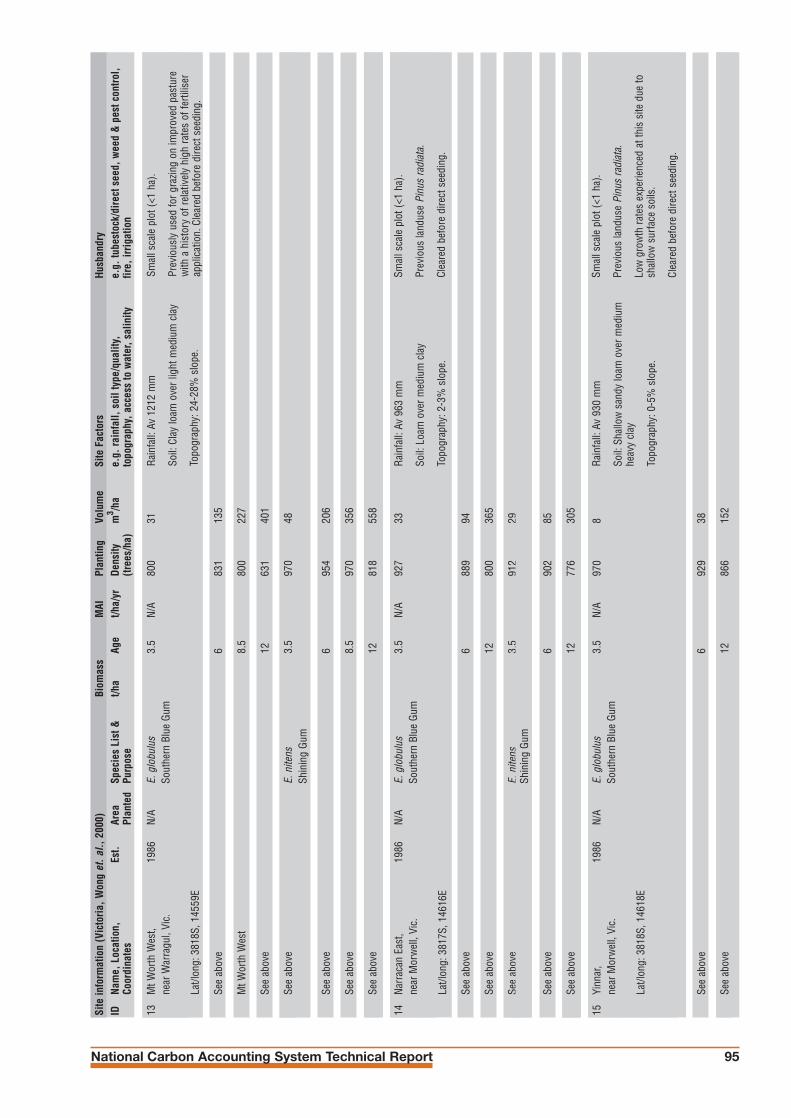
National Carbon Accounting System Technical Report 95
13M
t Wor
th W
est,
1986
N/A
E. g
lobu
lus
3.5
N/A
800
31ne
ar W
arra
gul,
Vic.
Sout
hern
Blu
e Gu
m
Lat/l
ong:
381
8S, 1
4559
E
See
abov
e6
831
135
Mt W
orth
Wes
t8.
580
022
7
See
abov
e12
631
401
See
abov
eE.
nite
ns3.
597
048
Shin
ing
Gum
See
abov
e6
954
206
See
abov
e8.
597
035
6
See
abov
e12
818
558
14Na
rrac
an E
ast,
1986
N/A
E. g
lobu
lus
3.5
N/A
927
33ne
ar M
orw
ell,
Vic.
Sout
hern
Blu
e Gu
m
Lat/l
ong:
381
7S, 1
4616
E
See
abov
e6
889
94
See
abov
e12
800
365
See
abov
eE.
nite
ns3.
591
229
Shin
ing
Gum
See
abov
e6
902
85
See
abov
e12
776
305
15Yi
nnar
,19
86N/
AE.
glo
bulu
s3.
5N/
A97
08
near
Mor
wel
l, Vi
c.So
uthe
rn B
lue
Gum
Lat/l
ong:
381
8S, 1
4618
E
See
abov
e6
929
38
See
abov
e12
866
152
Site
info
rmat
ion
(Vic
toria
, Won
g et
. al.,
200
0)Bi
omas
sM
AIPl
antin
gVo
lum
eSi
te F
acto
rsHu
sban
dry
ID
Nam
e, L
ocat
ion,
Es
t.Ar
ea
Spec
ies
List
&t/h
aAg
et/h
a/yr
Dens
ity
m3 /h
ae.
g. ra
infa
ll, s
oil t
ype/
qual
ity,
e.g.
tube
stoc
k/di
rect
see
d, w
eed
& p
est c
ontro
l,Co
ordi
nate
sPl
ante
dPu
rpos
e(tr
ees/
ha)
topo
grap
hy, a
cces
s to
wat
er, s
alin
ityfir
e, ir
rigat
ion
Rain
fall:
Av
963
mm
Soil:
Loa
m o
ver m
ediu
m c
lay
Topo
grap
hy: 2
-3%
slo
pe.
Smal
l sca
le p
lot (
<1 h
a).
Prev
ious
land
use
Pinu
s ra
diat
a.
Clea
red
befo
re d
irect
see
ding
.
Rain
fall:
Av
930
mm
Soil:
Sha
llow
san
dy lo
am o
ver m
ediu
mhe
avy
clay
Topo
grap
hy: 0
-5%
slo
pe.
Smal
l sca
le p
lot (
<1 h
a).
Prev
ious
land
use
Pinu
s ra
diat
a.
Low
gro
wth
rate
s ex
perie
nced
at t
his
site
due
tosh
allo
w s
urfa
ce s
oils
.
Clea
red
befo
re d
irect
see
ding
.
Rain
fall:
Av
1212
mm
Soil:
Cla
y lo
am o
ver l
ight
med
ium
cla
y
Topo
grap
hy: 2
4-28
% s
lope
.
Smal
l sca
le p
lot (
<1 h
a).
Prev
ious
ly u
sed
for g
razin
g on
impr
oved
pas
ture
with
a h
isto
ry o
f rel
ativ
ely
high
rate
s of
ferti
liser
appl
icat
ion.
Cle
ared
bef
ore
dire
ct s
eedi
ng.
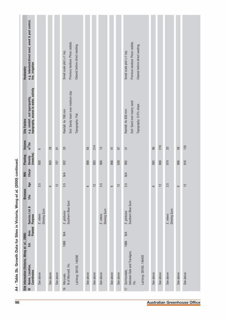
Australian Greenhouse Office96
See
abov
eE.
nite
ns3.
580
06
Shin
ing
Gum
See
abov
e6
803
28
See
abov
e12
707
81
16M
aryv
ale,
1986
N/A
E. g
lobu
lus
3.5
N/A
932
20N
of M
orw
ell,
Vic.
Sout
hern
Blu
e Gu
m
Lat/l
ong:
381
2S, 1
4628
E
See
abov
e6
888
65
See
abov
e12
883
214
See
abov
eE.
nite
ns3.
596
613
Shin
ing
Gum
See
abov
e6
966
41
See
abov
e12
638
87
17Go
rmon
dale
,19
86N/
AE.
glo
bulu
s3.
5N/
A99
231
betw
een
Sale
and
Tra
ralg
on,
Sout
hern
Blu
e Gu
mVi
c.
Lat/l
ong:
381
6S, 1
4642
E
See
abov
e6
992
86
See
abov
e12
868
216
See
abov
eE.
nite
ns3.
597
920
Shin
ing
Gum
See
abov
e6
966
58
See
abov
e12
916
135
Site
info
rmat
ion
(Vic
toria
, Won
g et
. al.,
200
0)Bi
omas
sM
AIPl
antin
gVo
lum
eSi
te F
acto
rsHu
sban
dry
ID
Nam
e, L
ocat
ion,
Es
t.Ar
ea
Spec
ies
List
&t/h
aAg
et/h
a/yr
Dens
ity
m3 /h
ae.
g. ra
infa
ll, s
oil t
ype/
qual
ity,
e.g.
tube
stoc
k/di
rect
see
d, w
eed
& p
est c
ontro
l,Co
ordi
nate
sPl
ante
dPu
rpos
e(tr
ees/
ha)
topo
grap
hy, a
cces
s to
wat
er, s
alin
ityfir
e, ir
rigat
ion
Rain
fall:
Av
768
mm
Soil:
San
dy lo
am o
ver m
ediu
m c
lay
Topo
grap
hy: F
lat.
Smal
l sca
le p
lot (
<1 h
a).
Prev
ious
land
use
Pinu
s ra
diat
a.
Clea
red
befo
re d
irect
see
ding
.
Rain
fall:
Av
830
mm
Soil:
San
d ov
er lo
amy
sand
Topo
grap
hy: 0
-5%
slo
pe.
Smal
l sca
le p
lot (
<1 h
a).
Prev
ious
land
use
Pinu
s ra
diat
a.
Clea
red
befo
re d
irect
see
ding
.
A4
- Ta
ble
2b
. Gro
wth
Dat
a fo
r S
ites
in V
icto
ria,
Wo
ng e
t al
.(20
00)
cont
inue
d.
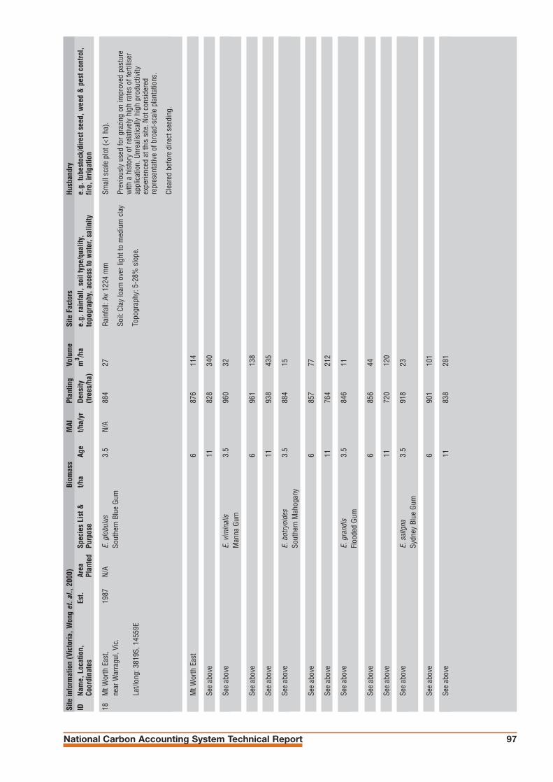
National Carbon Accounting System Technical Report 97
18M
t Wor
th E
ast,
1987
N/A
E. g
lobu
lus
3.5
N/A
884
27ne
ar W
arra
gul,
Vic.
Sout
hern
Blu
e Gu
m
Lat/l
ong:
381
9S, 1
4559
E
Mt W
orth
Eas
t6
876
114
See
abov
e11
828
340
See
abov
eE.
vim
inal
is3.
596
032
Man
na G
um
See
abov
e6
961
138
See
abov
e11
938
435
See
abov
eE.
bot
ryoi
des
3.5
884
15So
uthe
rn M
ahog
any
See
abov
e6
857
77
See
abov
e11
764
212
See
abov
eE.
gra
ndis
3.5
846
11Fl
oode
d Gu
m
See
abov
e6
856
44
See
abov
e11
720
120
See
abov
eE.
sal
igna
3.5
918
23Sy
dney
Blu
e Gu
m
See
abov
e6
901
101
See
abov
e11
838
281
Site
info
rmat
ion
(Vic
toria
, Won
g et
. al.,
200
0)Bi
omas
sM
AIPl
antin
gVo
lum
eSi
te F
acto
rsHu
sban
dry
ID
Nam
e, L
ocat
ion,
Es
t.Ar
ea
Spec
ies
List
&t/h
aAg
et/h
a/yr
Dens
ity
m3 /h
ae.
g. ra
infa
ll, s
oil t
ype/
qual
ity,
e.g.
tube
stoc
k/di
rect
see
d, w
eed
& p
est c
ontro
l,Co
ordi
nate
sPl
ante
dPu
rpos
e(tr
ees/
ha)
topo
grap
hy, a
cces
s to
wat
er, s
alin
ityfir
e, ir
rigat
ion
Rain
fall:
Av
1224
mm
Soil:
Cla
y lo
am o
ver l
ight
to m
ediu
m c
lay
Topo
grap
hy: 5
-28%
slo
pe.
Smal
l sca
le p
lot (
<1 h
a).
Prev
ious
ly u
sed
for g
razin
g on
impr
oved
pas
ture
with
a h
isto
ry o
f rel
ativ
ely
high
rate
s of
ferti
liser
appl
icat
ion.
Unr
ealis
tical
ly h
igh
prod
uctiv
ityex
perie
nced
at t
his
site
. Not
con
side
red
repr
esen
tativ
e of
bro
ad-s
cale
pla
ntat
ions
.
Clea
red
befo
re d
irect
see
ding
.
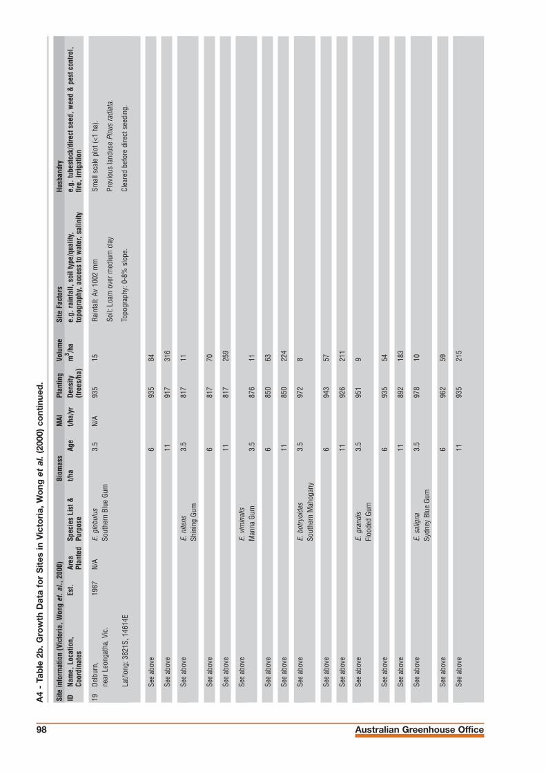
Australian Greenhouse Office98
19De
lbur
n,19
87N/
AE.
glo
bulu
s3.
5N/
A93
515
near
Leo
ngat
ha, V
ic.
Sout
hern
Blu
e Gu
m
Lat/l
ong:
382
1S, 1
4614
E
See
abov
e6
935
84
See
abov
e11
917
316
See
abov
eE.
nite
ns3.
581
711
Shin
ing
Gum
See
abov
e6
817
70
See
abov
e11
817
259
See
abov
eE.
vim
inal
isM
anna
Gum
3.5
876
11
See
abov
e6
850
63
See
abov
e11
850
224
See
abov
eE.
bot
ryoi
des
3.5
972
8So
uthe
rn M
ahog
any
See
abov
e6
943
57
See
abov
e11
926
211
See
abov
eE.
gra
ndis
3.5
951
9Fl
oode
d Gu
m
See
abov
e6
935
54
See
abov
e11
892
183
See
abov
eE.
sal
igna
3.5
978
10Sy
dney
Blu
e Gu
m
See
abov
e6
962
59
See
abov
e11
935
215
Site
info
rmat
ion
(Vic
toria
, Won
g et
. al.,
200
0)Bi
omas
sM
AIPl
antin
gVo
lum
eSi
te F
acto
rsHu
sban
dry
ID
Nam
e, L
ocat
ion,
Es
t.Ar
ea
Spec
ies
List
&t/h
aAg
et/h
a/yr
Dens
ity
m3 /h
ae.
g. ra
infa
ll, s
oil t
ype/
qual
ity,
e.g.
tube
stoc
k/di
rect
see
d, w
eed
& p
est c
ontro
l,Co
ordi
nate
sPl
ante
dPu
rpos
e(tr
ees/
ha)
topo
grap
hy, a
cces
s to
wat
er, s
alin
ityfir
e, ir
rigat
ion
A4
- Ta
ble
2b
. Gro
wth
Dat
a fo
r S
ites
in V
icto
ria,
Wo
ng e
t al
.(20
00)
cont
inue
d.
Rain
fall:
Av
1002
mm
Soil:
Loa
m o
ver m
ediu
m c
lay
Topo
grap
hy: 0
-8%
slo
pe.
Smal
l sca
le p
lot (
<1 h
a).
Prev
ious
land
use
Pinu
s ra
diat
a.
Clea
red
befo
re d
irect
see
ding
.
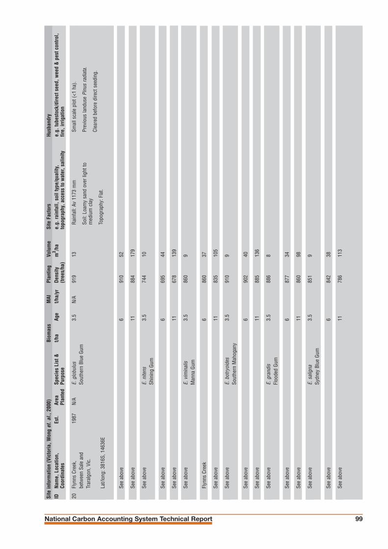
National Carbon Accounting System Technical Report 99
20Fl
ynns
Cre
ek,
1987
N/A
E. g
lobu
lus
3.5
N/A
919
13be
twee
n Sa
le a
nd
Sout
hern
Blu
e Gu
mTr
aral
gon,
Vic
.
Lat/l
ong:
381
6S, 1
4636
E
See
abov
e6
910
52
See
abov
e11
884
179
See
abov
eE.
nite
ns3.
574
410
Shin
ing
Gum
See
abov
e6
695
44
See
abov
e11
678
139
See
abov
eE.
vim
inal
is3.
586
09
Man
na G
um
Flyn
ns C
reek
686
037
See
abov
e11
835
105
See
abov
eE.
bot
ryoi
des
3.5
910
9So
uthe
rn M
ahog
any
See
abov
e6
902
40
See
abov
e11
885
136
See
abov
eE.
gra
ndis
3.5
886
8Fl
oode
d Gu
m
See
abov
e6
877
34
See
abov
e11
860
98
See
abov
eE.
sal
igna
3.5
851
9Sy
dney
Blu
e Gu
m
See
abov
e6
842
38
See
abov
e11
786
113
Site
info
rmat
ion
(Vic
toria
, Won
g et
. al.,
200
0)Bi
omas
sM
AIPl
antin
gVo
lum
eSi
te F
acto
rsHu
sban
dry
ID
Nam
e, L
ocat
ion,
Es
t.Ar
ea
Spec
ies
List
&t/h
aAg
et/h
a/yr
Dens
ity
m3 /h
ae.
g. ra
infa
ll, s
oil t
ype/
qual
ity,
e.g.
tube
stoc
k/di
rect
see
d, w
eed
& p
est c
ontro
l,Co
ordi
nate
sPl
ante
dPu
rpos
e(tr
ees/
ha)
topo
grap
hy, a
cces
s to
wat
er, s
alin
ityfir
e, ir
rigat
ion
Rain
fall:
Av
1173
mm
Soil:
Loa
my
sand
ove
r lig
ht to
med
ium
clay
Topo
grap
hy: F
lat.
Smal
l sca
le p
lot (
<1 h
a).
Prev
ious
land
use
Pinu
s ra
diat
a.
Clea
red
befo
re d
irect
see
ding
.
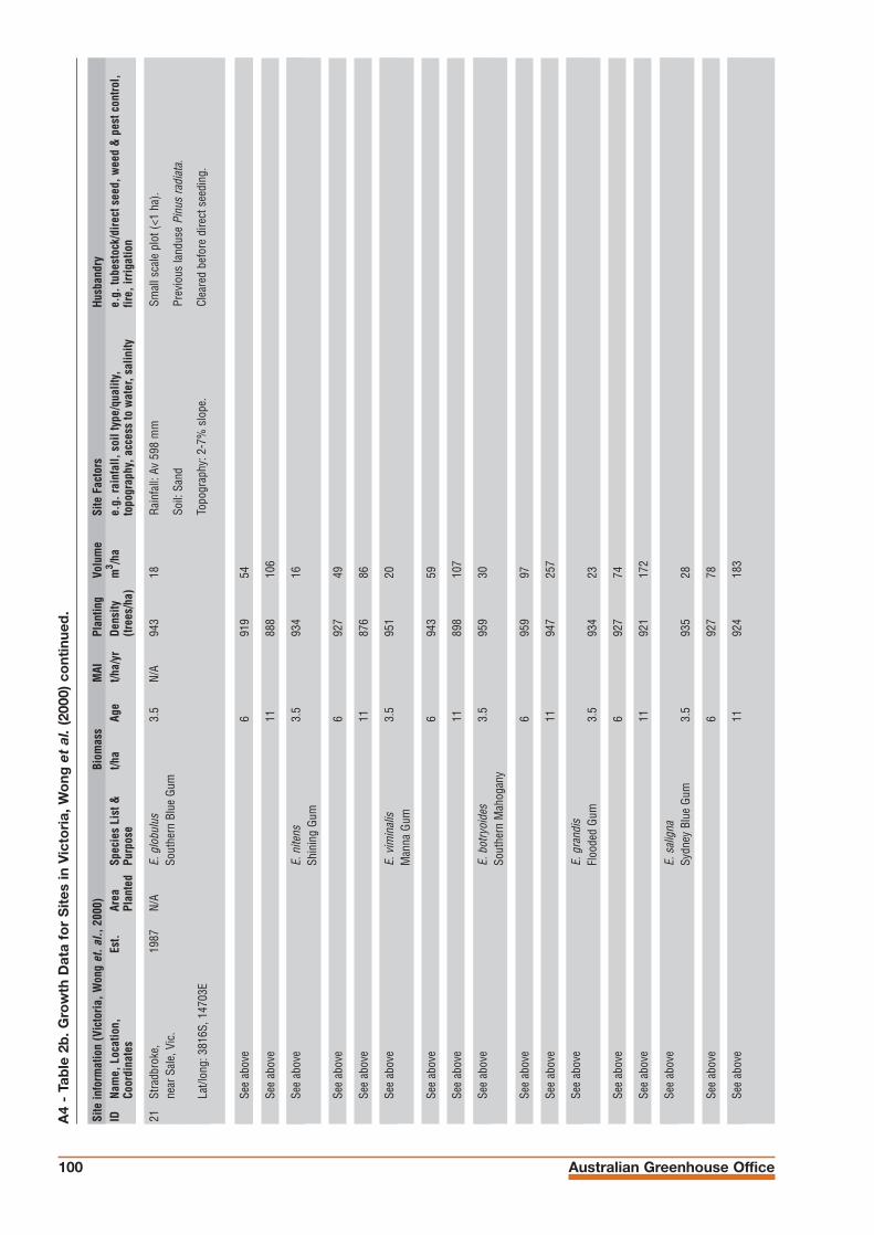
Australian Greenhouse Office100
21St
radb
roke
,19
87N/
AE.
glo
bulu
s3.
5N/
A94
318
near
Sal
e, V
ic.
Sout
hern
Blu
e Gu
m
Lat/l
ong:
381
6S, 1
4703
E
See
abov
e6
919
54
See
abov
e11
888
106
See
abov
eE.
nite
ns3.
593
416
Shin
ing
Gum
See
abov
e6
927
49
See
abov
e11
876
86
See
abov
eE.
vim
inal
is3.
595
120
Man
na G
um
See
abov
e6
943
59
See
abov
e11
898
107
See
abov
eE.
bot
ryoi
des
3.5
959
30So
uthe
rn M
ahog
any
See
abov
e6
959
97
See
abov
e11
947
257
See
abov
eE.
gra
ndis
Floo
ded
Gum
3.5
934
23
See
abov
e6
927
74
See
abov
e11
921
172
See
abov
eE.
sal
igna
Sydn
ey B
lue
Gum
3.5
935
28
See
abov
e6
927
78
See
abov
e11
924
183
Site
info
rmat
ion
(Vic
toria
, Won
g et
. al.,
200
0)Bi
omas
sM
AIPl
antin
gVo
lum
eSi
te F
acto
rsHu
sban
dry
ID
Nam
e, L
ocat
ion,
Es
t.Ar
ea
Spec
ies
List
&t/h
aAg
et/h
a/yr
Dens
ity
m3 /h
ae.
g. ra
infa
ll, s
oil t
ype/
qual
ity,
e.g.
tube
stoc
k/di
rect
see
d, w
eed
& p
est c
ontro
l,Co
ordi
nate
sPl
ante
dPu
rpos
e(tr
ees/
ha)
topo
grap
hy, a
cces
s to
wat
er, s
alin
ityfir
e, ir
rigat
ion
A4
- Ta
ble
2b
. Gro
wth
Dat
a fo
r S
ites
in V
icto
ria,
Wo
ng e
t al
.(20
00)
cont
inue
d.
Rain
fall:
Av
598
mm
Soil:
San
d
Topo
grap
hy: 2
-7%
slo
pe.
Smal
l sca
le p
lot (
<1 h
a).
Prev
ious
land
use
Pinu
s ra
diat
a.
Clea
red
befo
re d
irect
see
ding
.

National Carbon Accounting System Technical Report 101
22St
ockd
ale,
1987
N/A
E. g
lobu
lus
3.5
N/A
919
19N
of S
ale,
Vic
.So
uthe
rn B
lue
Gum
Lat/l
ong:
375
1S, 1
4711
E
See
abov
e6
902
61
See
abov
e11
877
141
See
abov
eE.
nite
ns3.
591
017
Shin
ing
Gum
See
abov
e6
893
52
See
abov
e11
679
84
See
abov
eE.
vim
inal
is3.
595
918
Man
na G
um
See
abov
e6
934
59
See
abov
e11
883
117
See
abov
eE.
bot
ryoi
des
3.5
919
15So
uthe
rn M
ahog
any
See
abov
e6
919
49
Stoc
kdal
e11
900
102
See
abov
eE.
gra
ndis
3.5
901
12Fl
oode
d Gu
m
See
abov
e6
901
43
See
abov
e11
876
89
See
abov
eE.
sal
igna
3.5
911
15Sy
dney
Blu
e Gu
m
See
abov
e6
893
48
See
abov
e11
829
98
Site
info
rmat
ion
(Vic
toria
, Won
g et
. al.,
200
0)Bi
omas
sM
AIPl
antin
gVo
lum
eSi
te F
acto
rsHu
sban
dry
ID
Nam
e, L
ocat
ion,
Es
t.Ar
ea
Spec
ies
List
&t/h
aAg
et/h
a/yr
Dens
ity
m3 /h
ae.
g. ra
infa
ll, s
oil t
ype/
qual
ity,
e.g.
tube
stoc
k/di
rect
see
d, w
eed
& p
est c
ontro
l,Co
ordi
nate
sPl
ante
dPu
rpos
e(tr
ees/
ha)
topo
grap
hy, a
cces
s to
wat
er, s
alin
ityfir
e, ir
rigat
ion
Rain
fall:
Av
1182
mm
Soil:
Loa
my
sand
ove
r med
ium
heav
ycl
ay
Topo
grap
hy: F
lat
Smal
l sca
le p
lot (
<1 h
a).
Prev
ious
land
use
Pinu
s ra
diat
a.
Clea
red
befo
re d
irect
see
ding
.

Australian Greenhouse Office102

National Carbon Accounting System Technical Report 103

Australian Greenhouse Office104
The National Carbon Accounting System:• Supports Australia's position in the international development of policyand guidelines on sinks activity and greenhouse gas emissionsmitigation from land based systems.
• Reduces the scientific uncertainties that surround estimates of landbased greenhouse gas emissions and sequestration in the Australian context.
• Provides monitoring capabilities for existing land based emissions andsinks, and scenario development and modelling capabilities thatsupport greenhouse gas mitigation and the sinks development agendathrough to 2012 and beyond.
• Provides the scientific and technical basis for internationalnegotiations and promotes Australia's national interests ininternational fora.
http://www.greenhouse.gov.au/ncas
For additional copies of this report phone 1300 130 606
Series 1 Publications
1. Setting the Frame
2. Estimation of Changes in Soil Carbon Due to Changes in Land Use
3. Woody Biomass: Methods for Estimating Change
4. Land Clearing 1970-1990: A Social History
5a. Review of Allometric Relationships for Estimating Woody Biomass for Queensland, the NorthernTerritory and Western Australia
5b. Review of Allometric Relationships for Estimating Woody Biomass for New South Wales, theAustralian Capital Territory, Victoria, Tasmania and South Australia
6. The Decay of Coarse Woody Debris
7. Carbon Content of Woody Roots: Revised Analysis and a Comparison with Woody ShootComponents (Revision 1)
8. Usage and Lifecycle of Wood Products
9. Land Cover Change: Specification for Remote Sensing Analysis
10. National Carbon Accounting System: Phase 1 Implementation Plan for the 1990 Baseline
11. International Review of the Implementation Plan for the 1990 Baseline (13-15 December 1999)
Series 2 Publications
12. Estimation of Pre-Clearing Soil Carbon Conditions
13. Agricultural Land Use and Management Information
14. Sampling, Measurement and Analytical Protocols for Carbon Estimation in Soil, Litter and CoarseWoody Debris
15. Carbon Conversion Factors for Historical Soil Carbon Data
16. Remote Sensing Analysis Of Land Cover Change - Pilot Testing of Techniques
17. Synthesis of Allometrics, Review of Root Biomass and Design of Future Woody BiomassSampling Strategies
18. Wood Density Phase 1 - State of Knowledge
19. Wood Density Phase 2 - Additional Sampling
20. Change in Soil Carbon Following Afforestation or Reforestation
21. System Design
22. Carbon Contents of Above-Ground Tissues of Forest and Woodland Trees
23. Developing a National Forest Productivity Model
24. Analysis of Wood Product Accounting Options for the National Carbon Accounting System
25. Review of Unpublished Biomass-Related Information: Western Australia, South Australia, NewSouth Wales and Queensland
26. CAMFor User Manual

national carbonaccounting system
tech
nica
l rep
ort n
o. 2
3
The National Carbon Accounting System provides a complete
accounting and forecasting capability for human-induced sources and
sinks of greenhouse gas emissions from Australian land based
systems. It will provide a basis for assessing Australia’s progress
towards meeting its international emissions commitments.
http://www.greenhouse.gov.au
technical report no. 23
Developing a NationalForest Productivity Model
Jenny Kesteven,Joe Landsberg andURS Australia
Developing a National Forest Productivity M
odel