development of a high-pressure rotational rheometer for
TRANSCRIPT
University of Calgary
PRISM: University of Calgary's Digital Repository
Graduate Studies The Vault: Electronic Theses and Dissertations
2018-01-08
Development of a High-pressure Rotational
Rheometer for Investigation of Effects of Dissolved
CO2
Lee, Keonje
Lee, K. (2018). Development of a High-pressure Rotational Rheometer for Investigation of Effects
of Dissolved CO2 (Unpublished master's thesis). University of Calgary, Calgary, AB.
http://hdl.handle.net/1880/106306
master thesis
University of Calgary graduate students retain copyright ownership and moral rights for their
thesis. You may use this material in any way that is permitted by the Copyright Act or through
licensing that has been assigned to the document. For uses that are not allowable under
copyright legislation or licensing, you are required to seek permission.
Downloaded from PRISM: https://prism.ucalgary.ca
UNIVERSITY OF CALGARY
Development of a High-pressure Rotational Rheometer for Investigation of
Effects of Dissolved CO2
by
Keonje Lee
A THESIS
SUBMITTED TO THE FACULTY OF GRADUATE STUDIES
IN PARTIAL FULFILMENT OF THE REQUIREMENTS FOR THE
DEGREE OF MASTER OF SCIENCE
GRADUATE PROGRAM IN MECHANICAL ENGINEERING
CALGARY, ALBERTA
JANUARY, 2018
© Keonje Lee 2018

ii
Abstract
Rheological information is often used to determine viscoelastic fluid properties, and to
model and predict fluid behavior under influence of external stress or deformation. Many
industrial processes involve the dissolution of gas under high pressure, so it is important to
evaluate the rheological properties of viscoelastic materials under high pressure. In this research,
a high pressure rotational rheometer was developed to measure the rheological parameters of
viscoelastic fluids and investigate the influence of the dissolution of gases on rheology. The
rheometer utilized a piezoelectric torque transducer, which enabled transient and dynamic
rheological measurements under high pressure. First, the rheometer was designed, fabricated,
and calibrated using a calibration fluid. Second, the capability of the rheometer was verified
using polydimethylsiloxane (PDMS), which is a typical viscoelastic fluid. Viscosity and
viscoelastic properties, such as storage/loss modulus, and complex viscosity, were evaluated.
Thirdly, the effects of the dissolved CO2 on the rheological properties of PDMS were
investigated. The effects of temperature and dissolved CO2 were investigated individually at the
temperature of 25, 50, 80°C and CO2 saturation pressures of 1, 2, 3 MPa. Then, the combined
effect was correlated using a generalized Arrhenius model. The proposed model expressed
viscosity as a function of temperature and pressure without the need for thermodynamic and
volumetric information of the fluid. The achievement of this research provides an alternative
method to measure rheological properties of viscoelastic materials under high pressure and
enables the prediction of the viscosity of a fluid with dissolved gas through modelling.
iii
Acknowledgements
The research undertaken for this thesis was conducted at the Mechanical and
Manufacturing Engineering department at the University of Calgary. This work would not have
been possible without the guidance of Dr. Simon Park, my supervisor who has been supportive
of my master’s program and career goals. He worked to provide me with continuous guidance,
encouragement and support to pursue those goals.
I would like to thank the supervisory committee members, Dr. Seonghwan Kim and Dr.
Joanna Wong, and external examiner, Dr. Giovanniantonio Natale for taking the time to review
this thesis. I would especially like to thank Dr. Giovanniantonio Natale for his professional
guidance in this research.
I am grateful to all of those with whom I have had the pleasure to work with during this
program. I would like to express my gratitude to my colleagues at the Micro Engineering
Dynamics and Automation Lab (MEDAL) for their assistance and friendship. I would especially
like to thank Mr. Allen Sandwell, Dr. Changyong Yim, Dr. Jongho Won, and Mr. Chaneel Park
for their assistance and support.

iv
Dedicated to my parents in Korea and Canada, my fiancé Gabrielle, and my sisters Jieun, Ann
and Yun for their love, endless support and sacrifices
v
Table of Contents
Abstract ......................................................................................................................... ii
Acknowledgements ....................................................................................................... iii
Table of Contents .......................................................................................................... v
List of Tables ................................................................................................................ vii
List of Figures ............................................................................................................... viii
List of Symbols ............................................................................................................. x
CHAPTER 1: INTRODUCTION ............................................................................... 1
1.1 Motivations ....................................................................................................... 3
1.2 Objectives ......................................................................................................... 5
1.3 Thesis Organization .......................................................................................... 8
CHAPTER 2: LITERATURE SURVEY .................................................................... 10
2.1 Viscoelasticity of Materials .............................................................................. 10
2.1.1 Newtonian and Non-Newtonian Fluid ..................................................... 12
2.1.2 Linear Viscoelasticity .............................................................................. 12
2.1.3 Linear Viscoelastic Models ...................................................................... 14
2.2 Rheological Measurement Techniques ............................................................. 16
2.2.1 Steady-shear ............................................................................................. 16
2.2.2 Sinusoidal Oscillation .............................................................................. 17
2.3 Rheometers ....................................................................................................... 19
2.3.1 Pressure-driven Rheometers .................................................................... 20
2.3.2 Drag Flow Rheometers ............................................................................ 22
2.3.3 High Pressure Rheometers ....................................................................... 27
2.4 Effects of Dissolved Gases on Rheology .......................................................... 33
2.4.1 Free Volume Theory ................................................................................ 34
2.4.2 Predictive Models Based on Free Volume Theory .................................. 34
2.5 Summary ........................................................................................................... 38
CHAPTER 3: EXPERIMENTAL SETUP .................................................................. 40
3.1 Design of Rotational Rheometer ....................................................................... 40
3.1.1 Overall Design ......................................................................................... 40
3.1.2 Piezoelectric Torque Dynamometer ........................................................ 43
3.1.3 Temperature Control ................................................................................ 44
3.1.4 Motion Control and Data Acquisition ...................................................... 46
3.1.5 Bearing and Dynamic Seal ....................................................................... 47
3.2 Materials Studied .............................................................................................. 48
3.3 Gap Optimization .............................................................................................. 49
3.4 Rheometer Calibration ...................................................................................... 51
3.4.1 Friction Compensation ............................................................................. 51
3.4.2 Calibration ................................................................................................ 56
3.4.3 Validation of Rheometer .......................................................................... 57
vi
3.5 Summary ........................................................................................................... 65
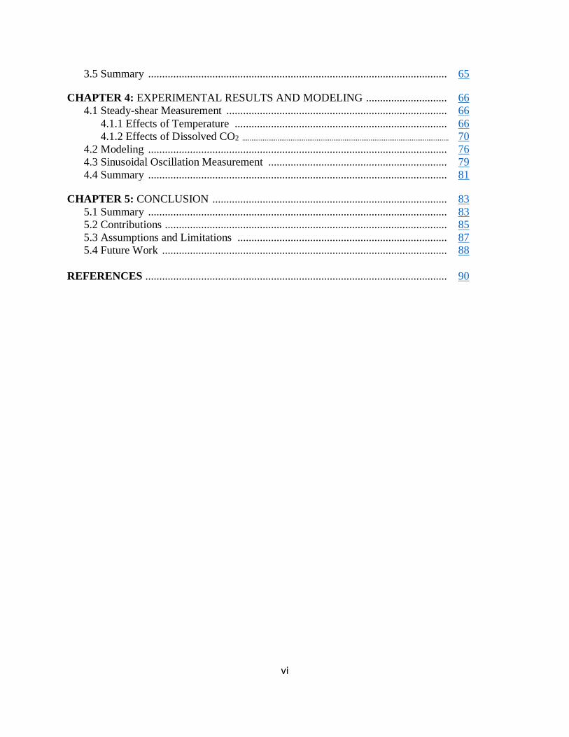
CHAPTER 4: EXPERIMENTAL RESULTS AND MODELING ............................. 66
4.1 Steady-shear Measurement ............................................................................... 66
4.1.1 Effects of Temperature ............................................................................ 66
4.1.2 Effects of Dissolved CO2 ............................................................................................................... 70
4.2 Modeling ........................................................................................................... 76
4.3 Sinusoidal Oscillation Measurement ................................................................ 79
4.4 Summary ........................................................................................................... 81
CHAPTER 5: CONCLUSION .................................................................................... 83
5.1 Summary ........................................................................................................... 83
5.2 Contributions ..................................................................................................... 85
5.3 Assumptions and Limitations ........................................................................... 87
5.4 Future Work ...................................................................................................... 88
REFERENCES ............................................................................................................ 90
vii
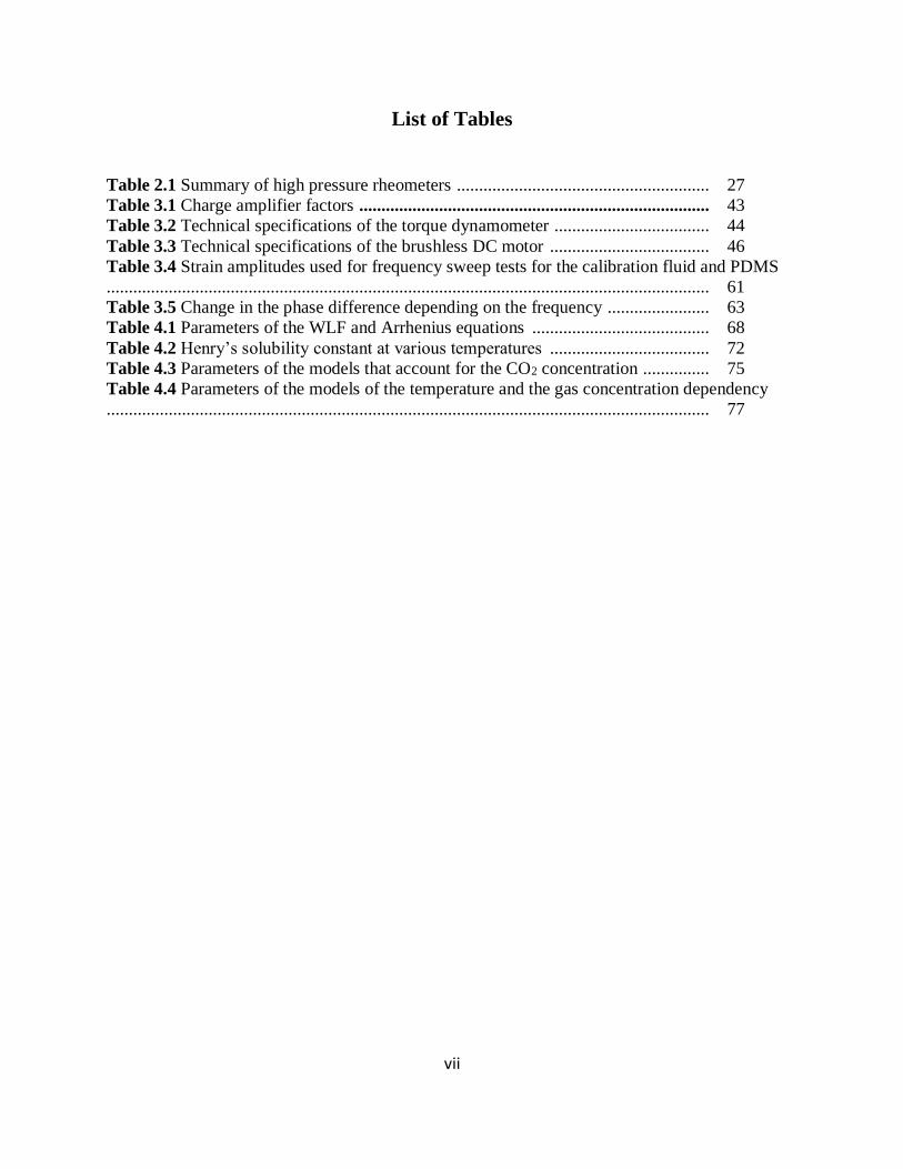
List of Tables
Table 2.1 Summary of high pressure rheometers ......................................................... 27
Table 3.1 Charge amplifier factors ............................................................................... 43
Table 3.2 Technical specifications of the torque dynamometer ................................... 44
Table 3.3 Technical specifications of the brushless DC motor .................................... 46
Table 3.4 Strain amplitudes used for frequency sweep tests for the calibration fluid and PDMS
........................................................................................................................................ 61
Table 3.5 Change in the phase difference depending on the frequency ....................... 63
Table 4.1 Parameters of the WLF and Arrhenius equations ........................................ 68
Table 4.2 Henry’s solubility constant at various temperatures .................................... 72
Table 4.3 Parameters of the models that account for the CO2 concentration ............... 75
Table 4.4 Parameters of the models of the temperature and the gas concentration dependency
........................................................................................................................................ 77

viii
List of Figures
Figure 2.1 Shear deformation ....................................................................................... 11
Figure 2.2 Stress response τ vs. time for step input in strain γ .................................... 13
Figure 2.3 Schematic of steady shear flow .................................................................. 17
Figure 2.4 Schematic of oscillatory shear flow ............................................................ 17
Figure 2.5 Strain and the resulting stress transducer signal in sinusoidal oscillation mode
........................................................................................................................................ 18
Figure 2.6 Schematic of a capillary rheometer (a) and the pressure and velocity profile in the
barrel ............................................................................................................................. 20
Figure 2.7 Schematic of a falling ball rheometer ......................................................... 23
Figure 2.8. Three common head geometries for a rotational rheometer: (a) concentric cylinders,
(b) cone and plate, and (c) parallel plates ..................................................................... 25
Figure 2.9 Schematic diagram of a falling-ball viscometer (Bae and Gulari 1997) .... 28
Figure 2.10 Schematic diagram of the high pressure chamber for the MLSR (Royer et al. 2002)
........................................................................................................................................ 29
Figure 2.11 Schematic of a capillary extrusion rheometer (Gerhardt et al. 1997) ....... 30
Figure 2.12 Schematic of an extruder with an on-line capillary rheometer (Lee et al. 1999)
........................................................................................................................................ 31
Figure 2.13 Schematic of (a) the high-temperature, high-pressure rheometer and (b) the cup-
spindle assembly (Khandare et al. 2000a) .................................................................... 33
Figure 3.1 Picture of the assembled rheometer ............................................................ 42
Figure 3.2 Schematic of the rheometer setup ................................................................ 42
Figure 3.3 Temperature set point vs. fluid temperature ................................................ 45
Figure 3.4 Elements of motion control and torque measurement ................................. 47
Figure 3.5 Theoretical estimation compared with experimental data of the total torque values
versus the distance of the parallel gap .......................................................................... 51
Figure 3.6 Torque as a function of shear rate due to system friction ............................ 53
Figure 3.7 Torque as a function of shear rate due to system friction ............................ 54
Figure 3.8 Torque correction scheme in steady shear mode ......................................... 55
Figure 3.9 Torque correction scheme in sinusoidal oscillation mode........................... 56
Figure 3.10 Calibration curve using the calibration fluid with a viscosity of 5,237 mPa·s
........................................................................................................................................ 57
Figure 3.11 Viscosity of the calibration fluid measured with and without the dynamic seal
........................................................................................................................................ 59
Figure 3.12 Viscosity of the PDMS measured with and without the dynamic seal ..... 59
Figure 3.13 Strain sweep test using the calibration fluid ............................................. 60
Figure 3.14 Strain sweep test using PDMS................................................................... 61
Figure 3.15 Storage and loss modulus (G’ and G’’) of the PDMS measured with and without the
dynamic seal................................................................................................................... 62
Figure 3.16 Magnitude of the complex viscosity (|𝜂*|) of the PDMS measured with and without
the dynamic seal ............................................................................................................. 64
Figure 4.1 Steady shear viscosity of pure PDMS as a function of shear rate at three temperatures
........................................................................................................................................ 67
Figure 4.2 Plot of -1/log(𝜂/𝜂0) vs. 1/(T-T0) to calculate the C1 and C2 from the experimental data
........................................................................................................................................ 68

ix
Figure 4.3 Plot of -ln(𝜂/𝜂0) vs. 1/R (T0-T) to calculate the E0 from the experimental data
........................................................................................................................................ 69
Figure 4.4 Viscosity of pure PDMS at various temperature with best-fit WLF and Arrhenius
correlations. The reference temperature, T0, is 25°C ..................................................... 69
Figure 4.5 Steady shear viscosity of PDMS-CO2 as a function of shear rate at various saturation
pressures ......................................................................................................................... 71
Figure 4.6 Equilibrium solubility of CO2 in PDMS at various temperatures (Xu et al. 2009)
........................................................................................................................................ 72
Figure 4.7 Plot of ln(H/H0) vs. 1/R (1/T-1/T0) to calculate the Es from the experimental data
........................................................................................................................................ 73
Figure 4.8 Viscosity of PDMS at various weight fraction of CO2 and 50°C along with several
predictive models. .......................................................................................................... 75
Figure 4.9 Plot of 1/ln(𝜂/cw,0 ) vs 1/wc as to calculate the f and 𝜃 from the experimental data
........................................................................................................................................ 75
Figure 4.10 Effect of the weight fraction of CO2 on relative viscosity of PDMS ........ 76
Figure 4.11 Viscosity as a function of temperature and pressure predicted using the generalized
Arrhenius equation ......................................................................................................... 78
Figure 4.12 Viscosity as a function of temperature and pressure predicted using the modified
generalized Arrhenius equation ..................................................................................... 78
Figure 4.13 Dynamic modulus of pure PDMS as a function of frequency at various temperatures
........................................................................................................................................ 79
Figure 4.14 Complex viscosity of pure PDMS as a function of frequency at various temperatures
........................................................................................................................................ 80
Figure 4.15 Dynamic modulus of pure PDMS as a function of frequency at various CO2
saturation pressures ........................................................................................................ 80
Figure 4.16 Complex viscosity of pure PDMS as a function of frequency at various CO2
saturation pressures ........................................................................................................ 81
x
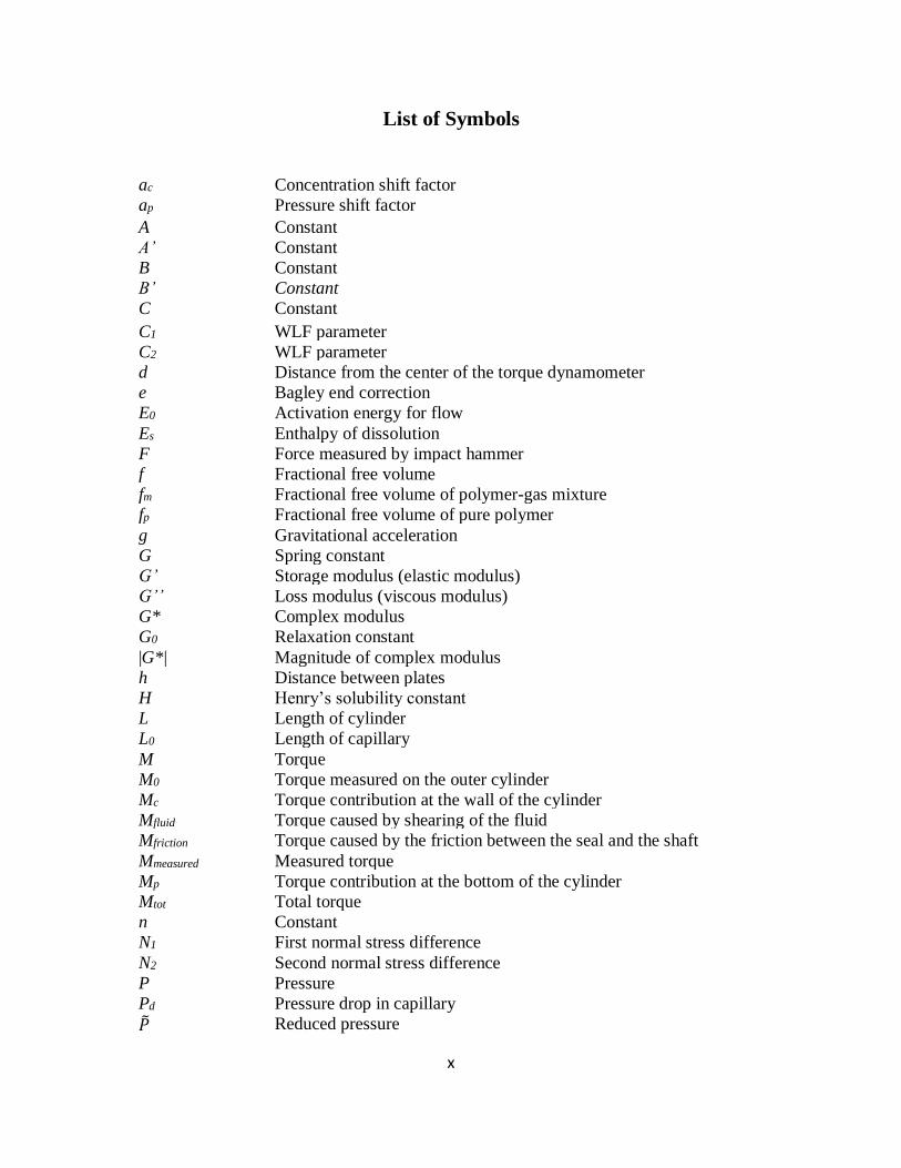
List of Symbols
ac Concentration shift factor
ap Pressure shift factor A Constant A’ Constant B Constant B’ Constant C Constant
C1 WLF parameter C2 WLF parameter d Distance from the center of the torque dynamometer e Bagley end correction E0 Activation energy for flow Es Enthalpy of dissolution F Force measured by impact hammer f Fractional free volume fm Fractional free volume of polymer-gas mixture fp Fractional free volume of pure polymer g Gravitational acceleration G Spring constant G’ Storage modulus (elastic modulus) G’’ Loss modulus (viscous modulus) G* Complex modulus G0 Relaxation constant |G*| Magnitude of complex modulus h Distance between plates H Henry’s solubility constant L Length of cylinder L0 Length of capillary M Torque M0 Torque measured on the outer cylinder Mc Torque contribution at the wall of the cylinder Mfluid Torque caused by shearing of the fluid Mfriction Torque caused by the friction between the seal and the shaft Mmeasured Measured torque Mp Torque contribution at the bottom of the cylinder Mtot Total torque n Constant N1 First normal stress difference N2 Second normal stress difference P Pressure Pd Pressure drop in capillary Reduced pressure

xi
q Effective polymer chain length Q Flow rate R Gas constant r Number of lattice sites occupied by a polymer chain Rb Radius of the ball Rc Radius of the capillary Ri Radius of the inner cylinder Ro Radius of the outer cylinder T Temperature t Time t’ Past time variable T0 Reference temperature Tfluid Temperature of fluid Tr Constant Tsp Temperature set-point Reduced temperature v∞ Terminal velocity Reduced volume Vm Specific volume of polymer-gas mixture Vp Specific volume of pure polymer wc Weight fraction of dissolved gas x Deformation at the top lane of a rectangular parallelepiped geometry y0 Height of a rectangular parallelepiped geometry Z Coordination number of the lattice 𝛼 Constant 𝛽 Constant 𝛾 Strain 𝛾0 Amplitude of strain Shear rate 𝐴 Apparent shear rate for a Newtonian fluid 𝑤 Shear rate on the wall
𝛿 Phase difference 𝜂 Viscosity (damping constant) 𝜂0 Viscosity at a reference temperature
𝜂0,𝑤𝑐 Viscosity of pure polymer
𝜂z Zero-shear viscosity |𝜂*| Magnitude of complex viscosity 𝜃 Parameter representing contribution of dissolved gas 𝜆 Relaxation time 𝜌b Density of the ball 𝜌f Density of the fluid Reduced density
𝜏 Shear stress 𝜏0 Amplitude of stress 𝜏w Shear stress on the wall

xii
𝜓 Constant 𝜓1 Normal stress coefficient 𝜓2 Normal stress coefficient 𝜔 Angular frequency Ω Angular velocity
1
CHAPTER 1: INTRODUCTION
Rheology is the study of stress and deformation of matter. It is an interdisciplinary field
that crosses over physics, chemistry, and several other disciplines. In fact, rheology is a
fundamental study that governs the mechanical deformation and flow of all pure and mixed
materials. There are various rheological parameters including viscosity, relaxation modulus,
storage modulus, loss modulus, complex viscosity, creep compliance, etc. Among these
rheological parameters, viscosity is the most widely used parameter, especially when flowability
of a material is a primary concern. It is well known that the viscosity of fluids is a critical
parameter in the hydraulic calculations of various systems including surface facilities, pipeline
systems, and flow through porous media (Monnery et al. 1995). Although viscosity provides
information on how fluids flow under steady shear, it does not sufficiently provide all the
necessary information to fully describe complex material behaviors under the transient or
dynamic change of strain or stress.
Response of viscoelastic materials under external stress or deformation is characterized
by rheological parameters such as relaxation modulus/spectrum and dynamic modulus. The
relaxation modulus is a measure of material response under transient strain over time. It has been
reported that the stress relaxation spectrum, which is a distribution of relaxation times, can be
used to estimate the molecular weight distribution by making assumptions in terms of the
functional relationship between molecular weight and relaxation time (Marin and Montfort 1996).
It is one of the fundamental ways to determine the viscoelasticity of materials; however, the use
of stress relaxation is limited to materials that have relatively long relaxation times due to
experimental challenges such as difficulty in measuring stress over time. The dynamic modulus,
2
which can be obtained from oscillatory measurements, is another important viscoelastic function
that is interchangeable with relaxation modulus. Both dynamic and relaxation modulus, as well
as other viscoelastic parameters, are correlated to one another and convertible to each other when
mathematical calculations are applied. By using these parameters, the molecular structure of
thermoplastic melts can be identified (Rohn 1995), and the crosslinking process of thermosetting
polymers can be monitored (Calvet et al. 2004). In other words, the aforementioned parameters
allow scientists and engineers to gain a fundamental understanding of the micro-structure and
flowability of materials.
Rheometers are instruments that measure the rheological parameters of materials, which
are fluids in most cases. They evaluate these parameters by measuring the stress induced as a
response to an applied strain or vice versa. Rheometers can be classified into two major
categories based on the way shear flow is generated: pressure drop and drag flow rheometers.
Pressure drop rheometers include capillary rheometers and slit-die extrusion rheometers. They
are used in processes where the shear is induced by pressure. Drag flow rheometers include
falling ball, parallel plate, and rotational rheometers. One major advantage of using a falling ball
rheometer is the simplicity of the system and the ease of applying high static pressure. However,
there is also a major disadvantage of this system: it is difficult to control stress and strain due to
the fixed dimensions and mass of the ball. Moreover, the flow field induced by the ball is very
complex causing difficulties in analyzing the flow. Rotational rheometers are the most versatile
types of rheometer because various stress or strain profiles can be imposed on a sample by
displacing the surface that is in contact with the sample. These are thus more suitable for
dynamic or transient measurements.
3
The development of various rheometers and advanced rheological techniques have
deepened the understanding of the flow properties of various fluids. Some of the industrial
sectors that benefit from these advancements include polymer/plastic, coatings/paints,
oil/petrochemical, geoscience, biomedical, and pharmaceutical industries. The heavy oil industry
is one of the major applications because the processes involved in the industry is largely affected
by the flow properties of heavy oil. Heavy oil does not flow as easily compared to other light
crude oils, thus posing several difficulties in terms of extraction from reservoirs and
transportation through pipelines.
Recently, injecting carbon dioxide (CO2) into a heavy oil reservoir has been drawing
attention in enhanced oil recovery due to its environmental and economic advantages. In addition
to displacing heavy oil from reservoir rock by building up pressure within the reservoir, injecting
CO2 also improves the rheological behavior of heavy oil by dissolving into the heavy oil under
high pressure. CO2 is highly soluble in heavy oil and is effective in viscosity reduction by
dissociating the micro-structure in heavy oil. Therefore, it is necessary to understand the
rheological behavior of heavy oil under high pressure and in the presence of dissolved CO2 to
optimize the process and better understand the micro phenomena associated with the dissolution
of CO2.
1.1 Motivations
Measuring the rheological parameters is essential in heavy oil industries because these
parameters are closely related to the flow of heavy oils. The most fundamental use of the
rheological data is to construct a mathematical model that describes the relationship between the
flow (deformation) and applied stress. This model is called a constitutive equation and can
4
predict the response of heavy oil under various histories of shear deformation. For example, the
linear and nonlinear viscoelastic behaviors of heavy oil have been modeled using constitutive
equations with rheological data collected from dynamic and stress relaxation experiments
(Behzadfar and Hatzikiriakos 2013). Rheological parameters also provide information on the
structure of heavy oil and how the structure affects the flow and vice versa. Many studies have
revealed that the intermolecular aggregation of asphaltene molecules are the major factor
contributing to the poor flowability of heavy oil, and the aggregation can be dissociated by
adding organic solvents or soluble gases (Pierre et al. 2004). Therefore, accurate and reliable
measurements of rheological parameters are of great importance.
Among the various type of rheometers, rotational rheometers are the most versatile and
able to perform various rheological measurement including dynamic measurements. For high
pressure applications, a magnetic coupling drive is often utilized to ensure the sample is
completely sealed off from the atmosphere, while torque is transferred to the rheometers. This
type of rheometer can eliminate the problems related to pressure gradients and non-homogeneity
within a sample because constant pressure throughout the sample can be achieved. Moreover,
because the flow field is known, shear stress and strain can be directly calculated from the
geometry and dimensions of the rheometer. Another advantage is that stress and strain are easily
manipulated by simply changing the speed or profile of the rotation. Various rheological tests
can be performed using rotational rheometers including steady shear, sinusoidal oscillation,
stress relaxation, and creep recovery. Although there are several advantages, these rheometers
are often difficult to design and fabricate. One of the main difficulties is in measuring the
dynamic torque. Torque is a primary measured variable in rotational rheometers and an accurate
measurement of torque is essential for accurate rheological measurements.

5
Traditionally, torque has been measured using a torsion bar/spring. The amount of
deflection of the torsion bar/spring is measured using a strain gauge. This method is still widely
used in rotational rheometers due to its simplicity and high sensitivity depending on the stiffness
of the bar/spring. The main drawback of the torsion bar/spring is that the deflection of the torsion
bar/spring causes an error in the strain imposed on the sample. Moreover, the low rigidity can
lead to a delay in the response to the applied strain and low resonance frequency; this delay can
result in a reduced range of transient or dynamic rheological testing. The problem of transducer
deflection can be eliminated by using a feedback control servo. The amount of current needed to
rotate the motor is proportional to the torque exerted on the fluid. However, the servo system
requires some time for feedback, which causes a delay in the torque measurement. Fast
acceleration or deceleration of the motor can also result in inaccurate torque measurements due
to the inertia of the motor and the spindle/shaft. Therefore, a torque measurement technique for
rotational rheometers that is more suitable for dynamic measurements should be explored.
Considering the limitations of the current high pressure rotational rheometers, using a
structurally rigid torque transducer with minimum inertial effect can significantly improve the
range of dynamic rheological measurements in rotational rheometers.
1.2 Objectives
The goal of this study is to investigate a new method to take rheological measurements of
viscoelastic fluids under high pressure that also involves the dissolution of a gas. This goal is
achieved by meeting the following specific aims:

6
i. Development of a rotational rheometer with a piezoelectric torque transducer
A rotational rheometer was designed, fabricated, and calibrated to measure the
rheological properties of viscoelastic fluids. The concentric cylinder is driven by a brushless DC
motor to impose the desired strain or strain rate exerting torque on the fluid in the rheometer.
Torque is measured using a piezoelectric torque transducer, which has a number of advantages
over other types of torque measurement techniques. First, it is rigid and, thus, has a higher
frequency bandwidth, resulting in more accurate measurements, especially in terms of dynamic
measurements. Second, the charge signal, which is the output of the transducer, is strictly
proportional to the load over a wide torque range.
Therefore, a wide range of dynamic viscosities can be accurately measured using the
piezoelectric torque transducer. The developed rheometer is equipped with a high pressure
dynamic shaft seal, which can be pressurized up to 3 MPa in the concentric cylinder; additionally,
a band heater is utilized to control the temperature up to 300°C. The developed rheometer is
calibrated using a calibration fluid to convert the torque to a corresponding shear stress.
ii. Investigation of rheological behavior of polymer melts
The capability of the developed rheometer is verified using a calibration fluid and PDMS
under ambient temperature and pressure. These two fluids represent a Newtonian fluid and a
non-Newtonian fluid that exhibit viscoelasticity. Their rheological behaviors are well known,
and therefore, they are used for the purpose of validation. Rheological measurements are
performed in steady shear and sinusoidal oscillation modes. In steady shear mode, shear stress is
measured at various shear rates and the shear viscosity is determined. In sinusoidal oscillation
mode, the amplitude of shear stress and phase difference are measured and the dynamic

7
rheological parameters, including storage modulus, G’, loss modulus, G’’, and complex viscosity,
|𝜂*|, are determined. Strain sweep tests are performed to determine the linear viscoelastic range
of PDMS, and frequency sweep tests are also performed to evaluate the dynamic rheological
parameters. Methods to compensate for the friction of the shaft seal are proposed, and the results
are compared to tests conducted without the shaft seal.
iii. Investigation of the effect of dissolved CO2 on the rheology of polymer melts and validation
through modeling
The effects of temperature, pressure, and dissolved CO2 on the rheological properties of
PDMS are investigated using the developed rheometer. Steady shear measurements are carried
out first at ambient pressure (without CO2) and various temperatures. Then, the effect of pressure
(thus, CO2 concentration) on viscosity is experimentally investigated at different temperatures.
After examining the effect of the individual parameters, the experimental results are then
correlated to a generalized Arrhenius model. Using this model, viscosity can be mathematically
expressed as a function of temperature and pressure without the need for thermodynamic
information, which is difficult to measure. Sinusoidal measurements are also conducted to
evaluate dynamic rheological parameters under the same conditions as the steady shear
measurement.
Through the completion of these objectives, a rheometer that can operate in pressurized
conditions will be developed. The developed rheometer will also be capable of performing
various rheological measurements in an increased dynamic range. The measurement error
associated with the compliance and inertia of torque transducers will be minimized. In addition,

8
the effect of various conditions, including temperature, pressure, and concentration of CO2, on
rheological parameters can be evaluated and predicted using the proposed model.
1.3 Thesis Organization
This thesis consists of five chapters including the introduction and is organized as follows:
Chapter 2 provides some theoretical background on rheology and the concept of linear
viscoelasticity. Various rheological measurement techniques and equations are also discussed.
Free volume theory and several predictive models based on this theory are introduced. Some of
the recent research on the development of rotational rheometers are summarized along with their
limitations.
The development of a high pressure rotational rheometer is described in Chapter 3. The
overall design and major sub-components of the rheometer are described in detail. A detailed
description of the rheological measurements, calculations, and friction compensation schemes
are presented. Some of the results of the preliminary tests using a calibration fluid and PDMS are
also presented.
The rheological properties of PDMS are investigated in Chapter 4 using the developed
rheometer. The effect of temperature and dissolved CO2 on the rheological parameters of PDMS
are studied in steady shear mode. Modeling of the viscosity using an empirical model is
presented in detail. The dynamic modulus (G’ and G’’) and complex viscosity (𝜂*) are
experimentally determined.
The last chapter, Chapter 5, concludes the presented work. A summary of the thesis and a
brief discussion of the results are provided. The novel contributions in the area of rheometer

9
development are discussed, followed by an explanation of the limitations and assumptions of the
presented work. This chapter concludes with recommendations for possible future work.
10
CHAPTER 2: LITERATURE SURVEY
In this chapter, the theoretical background on rheology is presented and relevant works
on rheometer development and high pressure rheology are reviewed. The difference between
Newtonian and non-Newtonian fluids is presented as well as the basic concepts and theoretical
background of linear viscoelasticity. Two rheological measurement techniques: steady shear and
sinusoidal oscillation, are described along with the rheological parameters that can be evaluated
using these techniques. Then, various types of rheometers, including ones that have been
designed or modified to accommodate high pressures, are introduced, and their pros and cons are
discussed. Experimental and theoretical studies on the effect of dissolved gas on viscosity
reduction are also discussed along with their associated predictive models.
2.1 Viscoelasticity of Materials
Rheology is the study of flow and deformation of materials under the influence of
stresses. It is often used to determine fluid properties and predict the behaviour of fluids. With
the recent wide-spread use of polymeric fluids, it is critical to achieve a method to study the
deformation and flow behaviours of time-dependent, semi-solid, or viscoelastic fluids.
Viscoelastic behaviour should be studied to expand our knowledge of the wide range of material
behaviours and the ultimate product performance.
Isaac Newton addressed the problem of steady flow in late 17th century in his famous
Principia Mathematica, which contains the hypothesis: "the resistance which arises from the lack
of slipperiness of the parts of the liquid, other things being equal, is proportional to the velocity
with which the parts of the liquid are separated from one another.” Newton’s “lack of

11
slipperiness” is now called viscosity. This concept is now scientifically described using shear
stress (𝜏) and shear strain (𝛾). A rectangular parallelepiped geometry, shown in Figure 2.1, is
subjected to a shear stress at the top plane while the bottom plane is stationary. The shear stress
the successive layer of the material to deform. Here, shear strain is defined as follows:
0
)(
y
tx (2.1)
where the height is y0 and deformation at the top plane is x(t). The rate of change in shear strain
is defined as strain rate () and can be expressed as:
dt
d (2.2)
Then, viscosity can be defined by the following mathematical expression:
(2.3)
Figure 2.1 Shear deformation
12
2.1.1 Newtonian and Non-Newtonian Fluids
Fluids can be classified as Newtonian or non-Newtonian depending on their shear stress
response to shear rate. Most fluids with a low molecular mass, such as water, organic solutions,
or gases, exhibit the characteristic that the shear stress is directly proportional to the shear rate at
a given temperature and pressure, leading to a constant viscosity. These fluids are classified as
Newtonian, named after Isaac Newton who first derived the relation between shear stress and
shear rate.
The most obvious deviation from Newtonian fluid behavior is that the flow curve does
not pass through the origin and/or is no longer linear. Therefore, for non-Newtonian fluids, the
viscosity, the slope of the flow curve, is not constant; rather it is a function of shear rate or shear
stress. Studies have also shown that the viscosity of a non-Newtonian fluid can depend on the
kinematic history of the fluid. These fluids are conveniently grouped into three general classes.
The first one includes the fluids whose shear rate, at any position of the fluid, is related only to
the value of the shear stress at that position at any given time. These fluids are usually called
“time-independent” fluids. The second class is for more complex fluids whose relationship
between shear stress and shear rate is a function of time, and they are called “time-dependent”
fluids. Finally, the third class is for the fluids that behave as a fluid under shear but as an elastic
solid at rest (infinite viscosity). They are categorized as “visco-plastic” fluids. Most real
materials illustrate a combination of these features under certain conditions.
2.1.2 Linear Viscoelasticity
Viscoelastic materials are materials whose relationship between stress and strain is time-
dependent. For example, when materials like silk, rubber, or glass are loaded in shear or

13
extension, an instantaneous deformation is followed by a continuous deformation (also known as
“creep”). When the load is removed, part of the deformation instantly recovers; some materials
completely recover with time, and other materials do not recover at all. Viscoelastic behavior is
typical of all polymeric materials. It is common to measure this phenomenon using stress
relaxation. An illustration of the behavior of viscoelastic materials compared to other materials is
shown in Figure 2.2.
Figure 2.2 Stress response τ vs. time for step input in strain γ
Figure 2.2 (a) shows the step input in strain, and figures 2.2 (b), (c), and (d) show the
stress response for different materials as a function of time. The Hookean solid (b) shows no
14
stress relaxation, and the Newtonian fluid (c) relaxes as soon as the strain is constant. In addition,
the viscoelastic material (d) shows stress relaxation over time. In a viscoelastic liquid, the stress
relaxes to zero, while in a viscoelastic solid, the stress approaches an asymptotic value (known as
equilibrium stress).
Linear viscoelastic materials display a linear relationship between stress relaxation and
strain at any given time. Linear viscoelasticity is a theory that describes the behavior of such
ideal materials. This theory is a reasonable approximation of the time-dependent behavior of
polymers, metals, and ceramics at relatively low temperatures and under relatively low stress.
For larger strains, the relaxation modulus is no longer independent of strain.
2.1.3 Linear Viscoelastic Models
Viscoelastic materials have properties of both viscous and elastic materials, represented
by Newtonian liquids and Hookean solids, respectively. Therefore, it is a reasonable approach to
express viscoelastic material responses as a combination of a dashpot and spring. This concept
has been the basis of various mechanical models of linear viscoelasticity. Stress (𝜏) of viscous
liquids and elastic solids in response to strain (𝛾) can be expressed as follows:
(2.4)
G (2.5)
where 𝜂 is the coefficient of viscosity and G is the shear modulus that have analogies with
damping and spring constant, respectively. If a dashpot and a spring are connected in parallel, the
total stress is the sum of the contributions of each element:
G (2.6)
15
The above equation is one of the simplest forms of a mechanical model called the Voigt model.
Another simple form is the Maxwell model where a dashpot and a spring are connected in series.
Then, the total strain rate (or strain) is the sum of the contributions of each element:
dt
d
G (2.7)
Other mechanical models are basically combinations of the Voigt and Maxwell models with a
spring and/or dashpot in series and/or parallel. For example, Zener (1944) proposed a three-
element mechanical model where a spring is added to the Voigt model in series or to the
Maxwell model in parallel. The Burger model is obtained by adding a spring or dashpot to the
Zener model. Almost an infinite number of models can be constructed by combining dashpots
and springs in various arrangement. However, one model that fits a certain material quite well
may not fit other materials. A more general model to represent the viscoelasticity of a material
can be constructed by connecting several Maxwell models in parallel, which is called the
generalized Maxwell model.
A single Maxwell model, which is given by the differential equation (2.7), can also be
expressed in the following form:
')'()( /)'(
0 dtteGt tt
t
(2.8)
where G0 is a relaxation constant, t’ is a past time variable, and 𝜆 = 𝜂/G is a relaxation time.
Then, the generalized Maxwell model with N number of Maxwell elements is expressed as the
sum of the single Maxwell models as follow:
t N
k
tt
k dtteGt k
1
/)'(')'()( (2.9)

16
This expression is useful in modeling most of the polymeric liquids and many other viscoelastic
materials. Although the individual elements may not have direct physical relation with the real
material, the combination of the elements can describe the linear viscoelastic behavior of
material quantitatively without the difficulties of going into mathematic in detail (Barnes et al.
1991).
2.2 Rheological Measurement Techniques
There are various ways to determine and measure the rheological properties of materials
using simple techniques. In this section, two rheological measurement techniques, steady shear
and sinusoidal oscillation, are discussed. These techniques are related to rheological parameters
such as viscosity, normal stress coefficients, storage and loss modulus, and complex viscosity.
2.2.1 Steady Shear
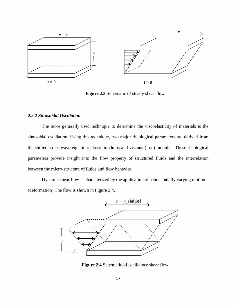
Steady shear flow is characterized by a continuously sheared fluid movement in one
direction as shown in Figure 2.3. A shear stress is generated as a response to the shearing, and
viscosity can be calculated as follows:
/ (2.10)
where is the shear stress, and is the shear rate. Viscosity can be expressed as a function of
shear rate and from this relationship, Newtonian and non-Newtonian behaviours, such as shear
thinning and thickening and yield stress, are distinguished. However, the viscous and elastic
responses of materials cannot be distinguished using this measurement technique.
17
Figure 2.3 Schematic of steady shear flow
2.2.2 Sinusoidal Oscillation
The more generally used technique to determine the viscoelasticity of materials is the
sinusoidal oscillation. Using this technique, two major rheological parameters are derived from
the shifted stress wave equation: elastic modulus and viscous (loss) modulus. These rheological
parameters provide insight into the flow property of structured fluids and the interrelation
between the micro-structure of fluids and flow behavior.
Dynamic shear flow is characterized by the application of a sinusoidally varying motion
(deformation) The flow is shown in Figure 2.4.
Figure 2.4 Schematic of oscillatory shear flow
h
t = 0
v = 0
t > 0
v
h
0
t sin0

18
Figure 2.5 Strain and the resulting stress transducer signal in sinusoidal oscillation mode
In general, an oscillatory measurement is a technique that is useful to evaluate the
viscoelastic properties of materials. Rheological parameters that can be evaluated from the
oscillatory measurement include the complex modulus (G*), storage modulus (G’), loss modulus
(G’’), and complex viscosity (𝜂*). When a sample is sheared sinusoidally at a certain amplitude
of strain and frequency, the resulting shear stress also oscillates in response to the applied strain
at the same frequency, but it is shifted by a certain phase angle depending on the material as
shown in Figure 2.5. This is expressed as follows:
t sin0 (2.11)
tsin0 (2.12)
where 𝛾0 is the amplitude of the strain, 𝜏0 is the amplitude of the stress, is the angular
frequency of the oscillation, and 𝛿 is the phase difference between the strain and stress wave.
The value of the phase difference, 𝛿, is 0 ° for an ideally elastic solid and 90 ° for an ideally
viscous liquid, and it is often expressed in the form of tan 𝛿, which is called loss tangent. The

19
phase shift of realistic materials falls between 0° and 90°. The stress, 𝜏, can be broken into two
sinusoidal waves: one is in phase and the other is out of phase by 90° with the strain wave.
tt cossin 00 (2.13)
Here, we can define two dynamic moduli: the storage modulus G’, which represents the elastic
portion of the complex shear modulus, and the loss modulus G’’, which represents the viscous
portion.
0
0
G (2.14)
0
0
G
(2.15)
Once the exact forms of the strain and stress are known, the rheological parameters can be easily
calculated using the following equations:
0
0
G (2.16)
cos GG (2.17)
sin GG (2.18)
G
(2.19)
2.3 Rheometers
A rheometer is an instrument used to characterize the rheology of a material. They are
classified into two main categories depending on how the shear is induced: pressure-driven
rheometers and drag flow rheometers.

20
2.3.1 Pressure-Driven Rheometers
Flow in pressure-driven rheometers is induced by a pressure difference along a hollow
die where the pressure is generated by gravity or a piston. The types of pressure driven
rheometers are defined by the geometry of the die; the most popular geometries are capillary
(cylindrical) and slit die (thin rectangular slit). Both types of rheometers have been widely used
to simulate processes such as polymer extrusion and pipeline transportation due to the similarity
of the flow. The schematic of a typical capillary rheometer is shown in Figure 2.6 (a).
Figure 2.6 Schematic of a capillary rheometer (a) and the pressure and velocity profile in the
barrel

21
Pressure drop and flow rate through the tube are measured variables in capillary
rheometers. Shear stress cannot be directly calculated, but pressure drop and flow rate should be
used with several assumptions to estimate the viscosity of fluids. The flow in the capillary is
nonhomogeneous thereby causing non-uniform shear stress and strain rate. Figure 2.6 (b) shows
the velocity profile in a capillary tube; shear rate is at a maximum at the wall and zero at the
center. Shear stress and shear rate at the wall should be determined. Bagley end correction is
often used to obtain shear stress on the wall (𝜏w) and can be expressed as follows:
eRL
P
c
dw
02 (2.20)
where Pd is the pressure drop in the capillary, L0 is the length of the capillary, Rc is the radius of
the capillary, and e is the Bagley end correction (Bagley 1957). Shear rate on the wall (𝑤) is
often determined by the Weissenberg-Rabinowitch equation as follows:
A
b
4
3 (2.21)
where
log
log
d
db A (2.22)
and 𝐴 is the apparent shear rate for a Newtonian fluid that can be expressed as follows:
3
4
c
AR
Q
(2.23)
where Q is the flow rate (Rabinowitsch 1929).
Capillary rheometers have numerous advantages over other type or rheometers. They are
the most accurate rheometer for measuring viscosity when a very long capillary is used, and they
are relatively inexpensive. The closed nature of the system and absence of any free surface
22
provides additional advantages including no solvent evaporation and no sample escaping from
the system, which often causes serious measurement errors in rotational rheometers. Although
the capillary rheometer is a good choice when used to evaluate steady shear rheological functions,
it cannot be used to measure dynamic or transient viscoelastic functions.
2.3.2 Drag Flow Rheometers
In drag flow rheometers, a sample is placed between two geometries and the shear is
induced by moving one geometry relative to another. The drag flow rheometers can operate
either in strain controlled and stress controlled mode. Although there are numerous variations of
drag flow rheometers, the most common types, falling ball, parallel plate, and rotational
rheometers, are discussed here.
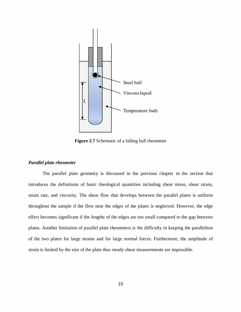
Falling ball rheometer
Falling ball rheometers measure the time required for a ball to fall a given distance in a
fluid. Different shear rates can be applied by using balls with different diameters or densities, or
by tilting the tube on an angle. However, these rheometers are rarely used for rheological studies
because the flow field induced by the ball is extremely complex and requires a constitutive
equation for complete analysis. Zero-shear viscosity is often reported because the flow is very
slow. The zero-shear viscosity (𝜂z) is expressed as follows:
9
22
bfb
z
gR (2.24)
where 𝜌b and 𝜌f are the density of the ball and the fluid, respectively, g is the gravitational
acceleration, Rb is the radius of the ball, and v∞ is the terminal velocity. The schematic of a
typical falling ball rheometer is shown in Figure 2.7.
23
Figure 2.7 Schematic of a falling ball rheometer
Parallel plate rheometer
The parallel plate geometry is discussed in the previous chapter in the section that
introduces the definitions of basic rheological quantities including shear stress, shear strain,
strain rate, and viscosity. The shear flow that develops between the parallel plates is uniform
throughout the sample if the flow near the edges of the plates is neglected. However, the edge
effect becomes significant if the lengths of the edges are too small compared to the gap between
plates. Another limitation of parallel plate rheometers is the difficulty in keeping the parallelism
of the two plates for large strains and for large normal forces. Furthermore, the amplitude of
strain is limited by the size of the plate thus steady shear measurements are impossible.

24
An attempt was made to mitigate the edge effect by developing a new rheometer.
Giacomin et al. (1989) developed a sliding plate rheometer with a beam type shear stress
transducer that was inserted into the middle of the plate to mitigate the edge effect.
Rotational rheometer
The most common type of rheometer is a rotational rheometer. In this configuration, a
sample is placed between two plates that rotate in relation to one another. Typically, one rotates
via electric motor, while the other plate serves as a torque transducer. Rotational rheometers are
used to characterize a variety of materials with a wide range of viscosities.
Different head geometries may be used in a shear mode rheometer to better accommodate
the material being tested. A few common head geometries are shown in Figure 2.8. The
concentric cylinder, also called a Couette, shown in Figure 2.8(a), is commonly used for very
low viscosity samples. This geometry is favorable because of its increased surface area compared
to other available options. The cone and plate configuration, Figure 2.8(b), is the most common
geometry used in rotational rheometers. This geometry provides the most consistent results and
is a convenient method for obtaining true viscosity. Parallel plates, shown in Figure 2.8(c), are
very similar to the cone and plate rheometer, except the flow between the parallel plates is not
homogeneous, which makes the calculation slightly more complicated. In this study, concentric
cylinder geometry was used for several reasons. First, since the focus in on the rheology of
bitumen at higher temperatures where the viscosity is significantly reduced, the concentric
cylinder would give more accurate measurements. Second, bitumen shows Newtonian behavior
above certain temperatures, so it is not necessary to characterize non-Newtonian rheological
properties such as normal force. Third, the concentric cylinder is much less sensitive to sample
loading error.

25
Figure 2.8. Three common head geometries for a rotational rheometer: (a) concentric cylinders,
(b) cone and plate, and (c) parallel plates
In addition, torque measurement techniques are a primary measured variable in rotational
rheometers, and the accurate measurement of torque is paramount for reliable rheological
measurements. A torsion bar/spring has been widely used for torque measurements in rotational
rheometers. The torsion bar/spring is attached to the inner or outer cylinder of the rotational
rheometer and deflects to certain angle depending on the torque exerted on it. The amount of
deflection is measured using a capacitance gage, linear variable differential transformer (LVDT),
optical device, etc. The measurement range depends on the stiffness of the torsion bar/spring
which means that an extremely small torque value can be accurately measured if a very thin
torsion bar is used. However, the issue with using torsion bar/spring is that they have low
resonant frequency, which reduces the range of transient or dynamic rheological measurements
(Macosko 1996). Moreover, the deflection of the torsion bar/spring leads to significant errors in
the strain or strain rate imposed on a fluid. Murata et al. (1987) developed a damped oscillation
26
rheometer consisting of a cylindrical tube suspended from a torsion wire that was filled with the
liquid to be tested. Karmakar and Kushwaha (2007) developed a rheometer to determine soil
visco-plastic parameters that work on the principle of torsional shear applied to a standard vane
with controlled strain rate.
Another torque measurement technique is using a feedback control servo. This technique
utilizes the motor drive current for torque measurements rather than using a separate torque
measurement unit. With the recent advances in automation and control, this technique has
become a popular way of measuring torque in rotational rheometers (Lauger 2008). It does not
require deflection of the components to measure torque. Moreover, the stress control mode can
be easily implemented with this method which enables the measurement of creep compliance
and yield stress of a material. The torque range is only limited by the size of the servo motor that
is being used. However, the response time of the servo system can cause delay and/or error in the
torque measurement. Even very well-tuned servo system takes time to stabilize. In addition, the
inertia of the shaft and spindle also causes erroneous measurement.
Considering the drawbacks associated with the current torque measurement techniques
used in rotational rheometers, a more reliable and accurate torque measurement technique is
needed. In this study, a piezoelectric torque transducer is used as an alternative method to
measure torque in rotational rheometers. The benefits of piezoelectric torque transducers
compared to the torsion bar/spring and the feedback control servo based torque transducers are
their higher resonance frequency and negligible transducer inertia due to their high stiffness.
Moreover, they have a high linearity over a wide range of torque values and are less sensitive to
temperature.

27
2.3.3 High Pressure Rheometers
Various industrial processes involve the flow of fluids under high pressure conditions.
Flow under high pressure is significantly different from the flow under ambient pressure and
sometimes involves the dissolution of gas which cause further change the rheological response of
a fluid.
High pressure rheometers are not significantly different from the above conventional
rheometers. They are often modification of the conventional rheometers to accommodate high
pressure in the system. High pressure in this context excludes hydraulic pressure, and only gas
pressure rheometers are discussed here. A summary of high pressure rheometers is presented in
Table 2.1.
Table 2.1 Summary of high pressure rheometers
Type Feature Researchers Year P (MPa) Tmax (°C) (𝒔−𝟏)
Falling ball Magnetic force Bae and
Gulari 1997 5 Room T N/A
Capillary Gerhardt et al. 1996 N/A N/A N/A
Capillary On-line Lee and Park 1999 N/A N/A N/A
Rotational Magnetic
coupling Oh et al. 2002 N/A N/A N/A
Rotational Magnetic
coupling
Khandare et
al. 2000 7.6 500
100 – 250
rpm
Rotatioanl Porous cup Wingert et al. 2009 20 N/A 10-7 – 1200
rpm
MLSR Magnetically
levitated sphere Royer et al. 2002 42 N/A 10-3 - 1
Falling ball rheometers can be easily modified for high pressure applications. Bae and
Gulari (1997) developed a high pressure falling ball viscometer to measure the viscosity of
PDMS-CO2 systems at elevated pressures up to 5 MPa. The schematic of the falling ball

28
viscometer is shown in the Figure 2.9. An inherent problem of falling ball rheometers is that
controlling the shear rate is difficult, because the shear rate is determined by the density and the
viscosity of the fluid. Moreover, the shear rate must be in the range of the Newtonian plateau.
Figure 2.9 Schematic diagram of a falling-ball viscometer (Bae and Gulari 1997)
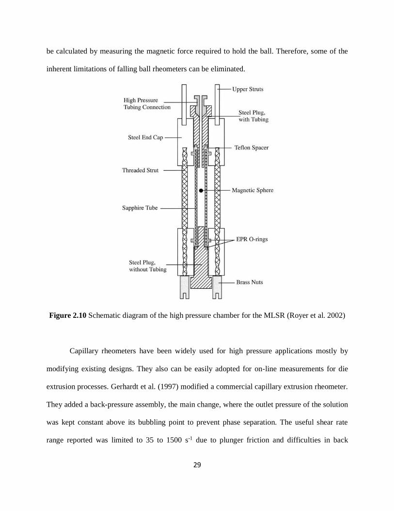
To overcome the drawbacks of conventional falling ball rheometers, Royer et al. (2002)
developed a magnetically levitated sphere rheometer (MLSR). The basic design of the developed
rheometer is very similar to a conventional falling ball rheometer as shown in Figure 2.10. In this
design, ball is held at a fixed position using magnetic levitation, while the sample cylinder that
contain the ball moves vertically using a motor to generate desired shear flow. Shear stress can
29
be calculated by measuring the magnetic force required to hold the ball. Therefore, some of the
inherent limitations of falling ball rheometers can be eliminated.
Figure 2.10 Schematic diagram of the high pressure chamber for the MLSR (Royer et al. 2002)
Capillary rheometers have been widely used for high pressure applications mostly by
modifying existing designs. They also can be easily adopted for on-line measurements for die
extrusion processes. Gerhardt et al. (1997) modified a commercial capillary extrusion rheometer.
They added a back-pressure assembly, the main change, where the outlet pressure of the solution
was kept constant above its bubbling point to prevent phase separation. The useful shear rate
range reported was limited to 35 to 1500 s-1 due to plunger friction and difficulties in back
30
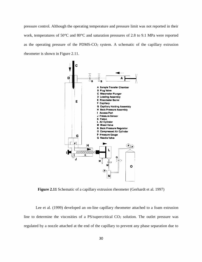
pressure control. Although the operating temperature and pressure limit was not reported in their
work, temperatures of 50°C and 80°C and saturation pressures of 2.8 to 9.1 MPa were reported
as the operating pressure of the PDMS-CO2 system. A schematic of the capillary extrusion
rheometer is shown in Figure 2.11.
Figure 2.11 Schematic of a capillary extrusion rheometer (Gerhardt et al. 1997)
Lee et al. (1999) developed an on-line capillary rheometer attached to a foam extrusion
line to determine the viscosities of a PS/supercritical CO2 solution. The outlet pressure was
regulated by a nozzle attached at the end of the capillary to prevent any phase separation due to
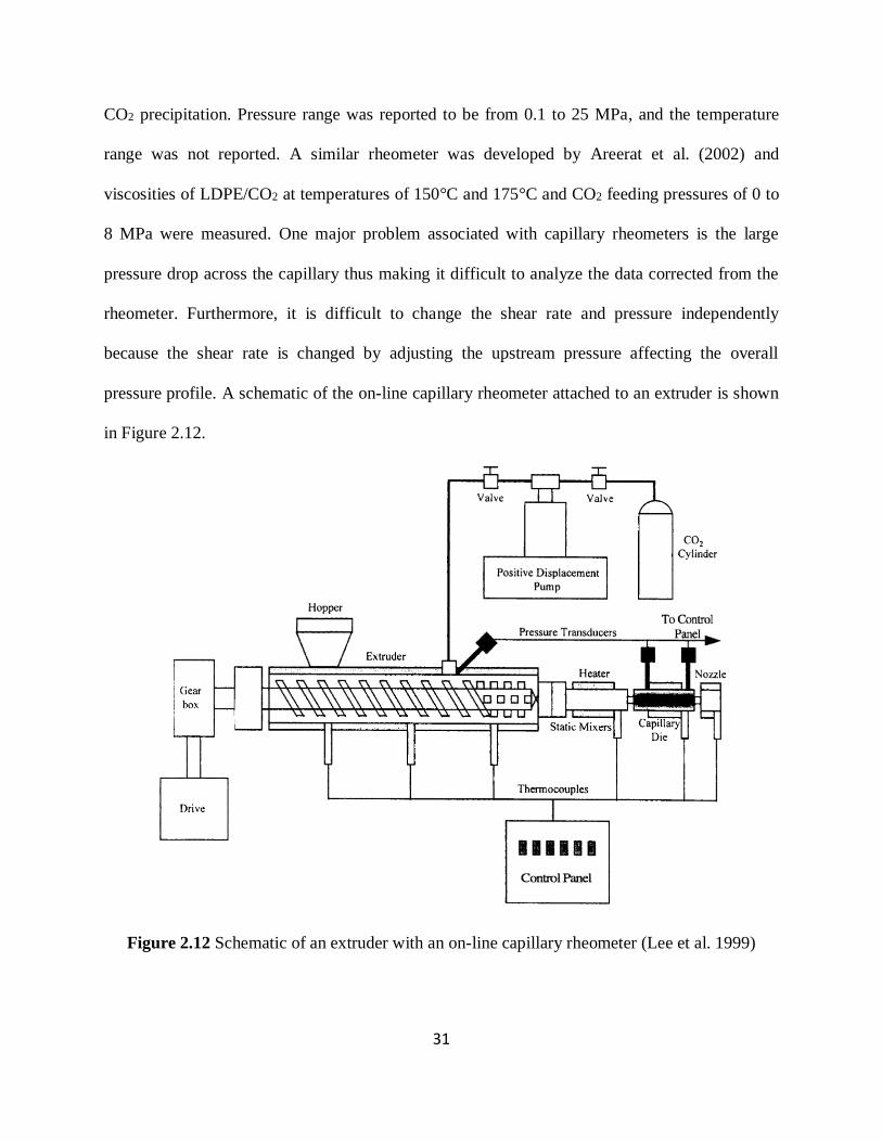
31
CO2 precipitation. Pressure range was reported to be from 0.1 to 25 MPa, and the temperature
range was not reported. A similar rheometer was developed by Areerat et al. (2002) and
viscosities of LDPE/CO2 at temperatures of 150°C and 175°C and CO2 feeding pressures of 0 to
8 MPa were measured. One major problem associated with capillary rheometers is the large
pressure drop across the capillary thus making it difficult to analyze the data corrected from the
rheometer. Furthermore, it is difficult to change the shear rate and pressure independently
because the shear rate is changed by adjusting the upstream pressure affecting the overall
pressure profile. A schematic of the on-line capillary rheometer attached to an extruder is shown
in Figure 2.12.
Figure 2.12 Schematic of an extruder with an on-line capillary rheometer (Lee et al. 1999)

32
This pressure gradient complexity can be eliminated using a rotational rheometer, which
can operate under static and saturated pressure. One major advantage of using rotational
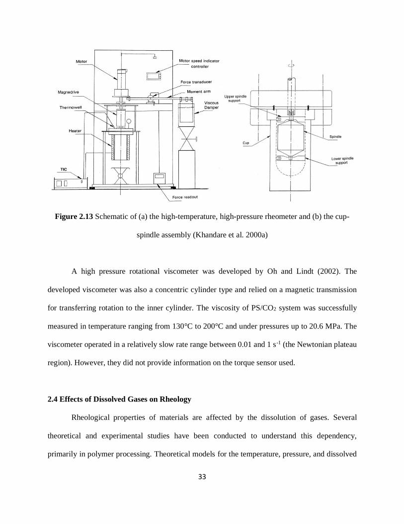
rheometers is that they can be used to study the viscoelasticity of fluids. A high temperature,
high pressure (HTHP) rotational rheometer was developed to measure the viscosities of pitch
materials at elevated temperatures and pressures (Khandare et al. 2000a). A schematic of the
HTHP rheometer is shown in Figure 2.13. The rheometer was a concentric cylinder type where
the inner cylinder was driven by a DC motor, and the torque exerted on the outer cylinder was
measured using a moment arm coupled with a linear variable differential transducer (LVDT). An
oil bath was utilized to reduce vibration and oscillation on the moment arm. The concentric
cylinder was built from a high pressure vessel with a magnetic coupling drive, which ensured
leak-free rotational motion. The maximum operating pressure and temperature was 7.6 MPa and
500°C, respectively. (Khandare et al. 2000a) determined the upper and lower boundaries of the
measurement range based on various factors including the magnetic drive torque limitation,
mechanical torque limitation, and flow instability due to Taylor vortices. Considering these
factors, the range of viscosity that could have been measured was between 10 and 500,000 mPa∙s.
They successfully measured the viscosity of carbonaceous pitch material at various temperatures
and shear rates and validated the experimental results with commercial viscometers (Khandare et
al. 2000b). Although they named it as a rheometer, the only rheological parameter reported was
viscosity. This reason seemed to be attributed to the low compliance and rigidity of the moment
arm, which was only suitable for steady shear measurements. Moreover, they did not present any
high pressure rheological measurements using the developed rheometer.
33
Figure 2.13 Schematic of (a) the high-temperature, high-pressure rheometer and (b) the cup-
spindle assembly (Khandare et al. 2000a)
A high pressure rotational viscometer was developed by Oh and Lindt (2002). The
developed viscometer was also a concentric cylinder type and relied on a magnetic transmission
for transferring rotation to the inner cylinder. The viscosity of PS/CO2 system was successfully
measured in temperature ranging from 130°C to 200°C and under pressures up to 20.6 MPa. The
viscometer operated in a relatively slow rate range between 0.01 and 1 s-1 (the Newtonian plateau
region). However, they did not provide information on the torque sensor used.
2.4 Effects of Dissolved Gases on Rheology
Rheological properties of materials are affected by the dissolution of gases. Several
theoretical and experimental studies have been conducted to understand this dependency,
primarily in polymer processing. Theoretical models for the temperature, pressure, and dissolved

34
gas dependency that have been developed based on the free volume theory are discussed in this
chapter.
2.4.1 Free Volume Theory
Doolittle’s free volume theory (Doolittle 1951) described the effects of free volume on
the viscosity of polymers. Doolittle’s free volume equation is as follows:
f
BA
''lnln (2.25)
where 𝜂 is viscosity, f is the fractional free volume, and A’ and B’ are constants. Although it was
originally developed to describe the temperature dependency on the viscosity of polymers, it has
been found that the effect of other variables, such as pressure and diluent concentration, can be
explained and described by the free volume concept.
2.4.2 Predictive Models Based on Free Volume Theory
Classical viscoelastic scaling methods, which employed a composition-dependent shift
factor to scale both viscosity and shear rate, were used to reduce the viscosity data of the PDMS-
CO2 system to a master curve at each temperature (Gerhardt et al. 1997). Gerhardt et al.
demonstrated that the main mechanism of the viscosity reduction upon the dissolution of gas
involved both the dilution effect and an increase in free volume by comparing the PDMS-CO2
system and the iso-free volume dilation.
The Kelly and Bueche equation was originally developed to express the viscosity of
concentrated polymer solutions, based on Doolittle’s free volume equation (Kelley and Bueche
1961). Gerhardt et al. (1998) modified this equation to describe the viscosities of PDMS-CO2
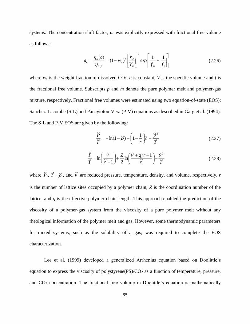
35
systems. The concentration shift factor, ac was explicitly expressed with fractional free volume
as follows:
pm
n
m
pn
c
po
oc
ffV
Vw
ca
11exp)1(
)(
,
(2.26)
where wc is the weight fraction of dissolved CO2, n is constant, V is the specific volume and f is
the fractional free volume. Subscripts p and m denote the pure polymer melt and polymer-gas
mixture, respectively. Fractional free volumes were estimated using two equation-of-state (EOS):
Sanchez-Lacombe (S-L) and Panayiotou-Vera (P-V) equations as described in Garg et al. (1994).
The S-L and P-V EOS are given by the following:
T
p
rT
P~
~~1
1)~1ln(~
~ 2
(2.27)
T
rqZ
T
P~~
1~ln
21~
~ln~
~ 2
(2.28)
where P~
, T~
, ~ , and v~ are reduced pressure, temperature, density, and volume, respectively, r
is the number of lattice sites occupied by a polymer chain, Z is the coordination number of the
lattice, and q is the effective polymer chain length. This approach enabled the prediction of the
viscosity of a polymer-gas system from the viscosity of a pure polymer melt without any
rheological information of the polymer melt and gas. However, some thermodynamic parameters
for mixed systems, such as the solubility of a gas, was required to complete the EOS
characterization.
Lee et al. (1999) developed a generalized Arrhenius equation based on Doolittle’s
equation to express the viscosity of polystyrene(PS)/CO2 as a function of temperature, pressure,
and CO2 concentration. The fractional free volume in Doolittle’s equation is mathematically
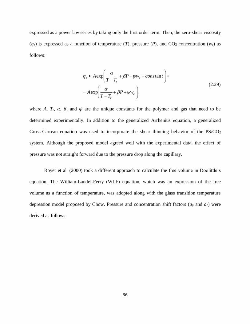
36
expressed as a power law series by taking only the first order term. Then, the zero-shear viscosity
(𝜂z) is expressed as a function of temperature (T), pressure (P), and CO2 concentration (wc) as
follows:
.exp
tanexp
c
r
c
r
z
wPTT
A
tconswPTT
A
(2.29)
where A, Tr, 𝛼, 𝛽, and 𝜓 are the unique constants for the polymer and gas that need to be
determined experimentally. In addition to the generalized Arrhenius equation, a generalized
Cross-Carreau equation was used to incorporate the shear thinning behavior of the PS/CO2
system. Although the proposed model agreed well with the experimental data, the effect of
pressure was not straight forward due to the pressure drop along the capillary.
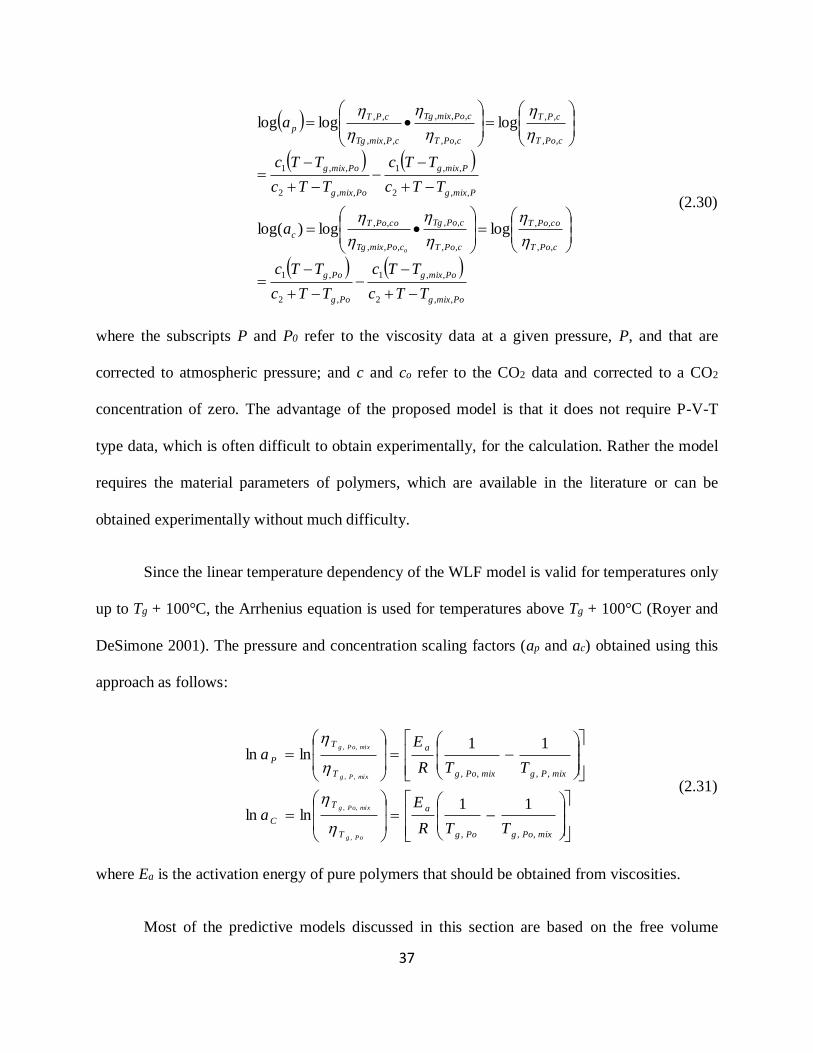
Royer et al. (2000) took a different approach to calculate the free volume in Doolittle’s
equation. The William-Landel-Ferry (WLF) equation, which was an expression of the free
volume as a function of temperature, was adopted along with the glass transition temperature
depression model proposed by Chow. Pressure and concentration shift factors (ap and ac) were
derived as follows:
37
Pomixg
Pomixg
Pog
Pog
cPoT
coPoT
cPoT
cPoTg
cPomixTg
coPoT
c
Pmixg
Pmixg
Pomixg
Pomixg
cPoT
cPT
cPoT
cPomixTg
cPmixTg
cPT
p
TTc
TTc
TTc
TTc
a
TTc
TTc
TTc
TTc
a
o
,,2
,,1
,2
,1
,,
,,
,,
,,
,,,
,,
,,2
,,1
,,2
,,1
,,
,,
,,
,,,
,,,
,,
loglog)log(
logloglog
•
•
(2.30)
where the subscripts P and P0 refer to the viscosity data at a given pressure, P, and that are
corrected to atmospheric pressure; and c and co refer to the CO2 data and corrected to a CO2
concentration of zero. The advantage of the proposed model is that it does not require P-V-T
type data, which is often difficult to obtain experimentally, for the calculation. Rather the model
requires the material parameters of polymers, which are available in the literature or can be
obtained experimentally without much difficulty.
Since the linear temperature dependency of the WLF model is valid for temperatures only
up to Tg + 100°C, the Arrhenius equation is used for temperatures above Tg + 100°C (Royer and
DeSimone 2001). The pressure and concentration scaling factors (ap and ac) obtained using this
approach as follows:
mixPogPog
a
T
T
C
mixPgmixPog
a
T
T
P
TTR
Ea
TTR
Ea
Pog
mixPog
mixPg
mixPog
,,,
,,,,
11lnln
11lnln
,
,,
,,
,,
(2.31)
where Ea is the activation energy of pure polymers that should be obtained from viscosities.
Most of the predictive models discussed in this section are based on the free volume
38
theory. The problem associated with this theory is that it requires information on the volumetric
parameters and thermodynamic properties of the gas, polymer, and mixture, and these
parameters and properties are difficult to measure. Therefore, a predictive model that is easily
applicable to polymer-gas systems is required. In this thesis, the generalized Arrhenius equation
used by Lee et al. is modified and used to predict the viscosity of a PDMS-CO2 system. The
concentration of CO2 in equation (2.29) is expressed as a function of temperature and pressure,
so the viscosity can also be expressed as a function of temperature and pressure without the need
for difficult thermodynamic calculations.
2.5 Summary
This chapter presented the theoretical background on rheology and viscoelasticity,
various types of rheometers with their pros and cons, and high pressure rheometers that were
developed to investigate polymer-gas rheology. A literature review of experimental and
theoretical studies on polymer-gas rheology was also presented.
Pressure driven rheometers have been extensively used in polymer processing and
pipeline engineering because of the similarity in the flow. However, the large pressure drop
across the capillary or slit die limits the amount of gas dissolved in the fluid and causes non-
uniformity within the sample. Falling ball rheometers also have also been widely used for high
pressure rheological measurements due to their simple design and ease of operation. However,
the shear flow induced by the ball is highly complex and difficult to analyze. Rotational
rheometers can eliminate the problems related to pressure gradients and non-homogeneity
because constant pressure throughout the sample can be achieved. Moreover, various rheological
parameters can be measured using rotational rheometers.
39
Although several other studies have also developed rheometers, most of these rheometers
have been torsion-based rather than torque-based. Even relatively stiff torsion bars must twist a
little to record the torque, which can lead to significant errors in the strain or transient strain rate
imposed on a sample. Therefore, in this study, a piezoelectric torque transducer, which is more
rigid and thus has a higher resonant frequency, resulting in more accurate measurements, is used
for torque measurement. Furthermore, the developed rheometer can determine not only viscosity,
but also a wide range of other rheological properties, including G’ (the storage modulus) and G’’
(the loss modulus).
40
CHAPTER 3: EXPERIMENTAL SETUP
In this chapter, the design and implementation of the high pressure rotational rheometer is
discussed. The novel design features of the developed rheometer are the utilization of a
piezoelectric torque dynamometer and a high pressure dynamic seal both of which enable
dynamic rheological measurements under pressurized gases. The overview of the design and the
core components, including the piezoelectric torque dynamometer and charge amplifier, band
heater and temperature controller, servo motor and motion controller, and bearing and dynamic
seal, are discussed. Then, the materials (calibration fluid, PDMS, and CO2) used for the
rheological measurements are presented. The effect of the bottom plate gap is investigated to
find the optimum gap where the end effect becomes negligible. Finally, the overall system is
calibrated using the calibration fluid, and the methods for compensating and/or mitigating
friction of the dynamic seal are presented.
3.1 Design of Rotational Rheometer
3.1.1 Overall Design
The developed rheometer is a rotational rheometer with concentric cylinders that shears a
sample between the inner (i.e., bob) and the outer (i.e., cup) cylinder. Concentric cylinder
geometry was chosen over other possible options because it is less sensitive to the sample
volume, and therefore, it is less effected by sample loading errors and swelling due to the
dissolution of gas. Further, concentric cylinder geometry makes more contact with a sample
compared to the cone and plate and parallel plates geometry resulting in much higher torque
imposed on a sample and more accurate rheological measurements.
41
The experimental setup and schematic of the developed rheometer are illustrated in
Figure 3.17 and Figure 3.18. The rheometer is primarily a custom-designed vessel of ~50 mL
capacity with a mechanical agitator mounted on a highly sensitive piezoelectric torque
dynamometer. The mechanical agitator consists of a brushless DC motor, rotating shaft, and a
cylindrical geometry that is attached to the end of the shaft. The motor is coupled with a
differential encoder to track the exact position and velocity of the shaft. A single-axis motion
controller with a software package provided by the manufacturer enabled the motor to operate in
the desired manner. The dynamic seal used for the rotating shaft is a polytetrafluoroethylene
(PTFE) lip seal with a stainless-steel U-spring. The vessel is also equipped with a gas inlet and
outlet, a pressure gauge, and a rupture disc with a 700 psi pressure rating for high pressure
experiments. The reactor is heated using a band heater, and the temperature is controlled using a
benchtop temperature controller (Omega CSi32) coupled with a K-type thermocouple attached to
the outer wall of the reactor. When the fluid inside the reactor is sheared by a rotation of the rotor,
torque is exerted to the inner wall of the reactor depending on the rheological response of the
fluid. This torque is measured at the piezoelectric torque dynamometer.

42
Figure 3.17 Picture of the assembled rheometer
Figure 3.18 Schematic of the rheometer setup
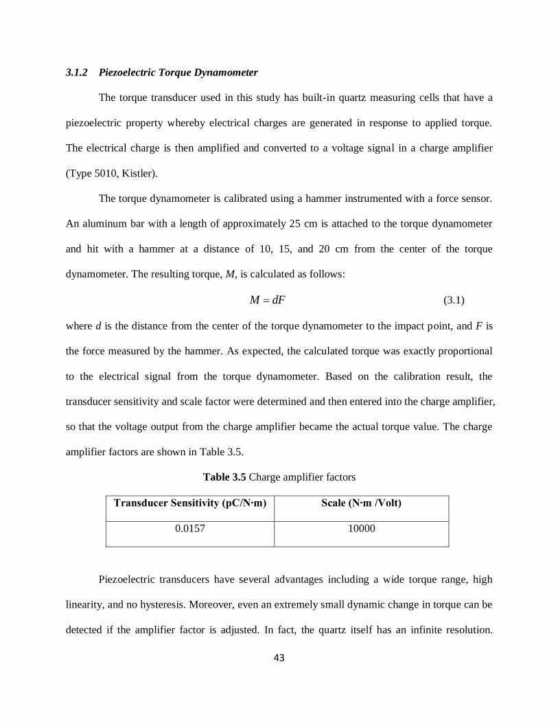
43
3.1.2 Piezoelectric Torque Dynamometer
The torque transducer used in this study has built-in quartz measuring cells that have a
piezoelectric property whereby electrical charges are generated in response to applied torque.
The electrical charge is then amplified and converted to a voltage signal in a charge amplifier
(Type 5010, Kistler).
The torque dynamometer is calibrated using a hammer instrumented with a force sensor.
An aluminum bar with a length of approximately 25 cm is attached to the torque dynamometer
and hit with a hammer at a distance of 10, 15, and 20 cm from the center of the torque
dynamometer. The resulting torque, M, is calculated as follows:
dFM (3.1)
where d is the distance from the center of the torque dynamometer to the impact point, and F is
the force measured by the hammer. As expected, the calculated torque was exactly proportional
to the electrical signal from the torque dynamometer. Based on the calibration result, the
transducer sensitivity and scale factor were determined and then entered into the charge amplifier,
so that the voltage output from the charge amplifier became the actual torque value. The charge
amplifier factors are shown in Table 3.5.
Table 3.5 Charge amplifier factors
Transducer Sensitivity (pC/N∙m) Scale (N∙m /Volt)
0.0157 10000
Piezoelectric transducers have several advantages including a wide torque range, high
linearity, and no hysteresis. Moreover, even an extremely small dynamic change in torque can be
detected if the amplifier factor is adjusted. In fact, the quartz itself has an infinite resolution.
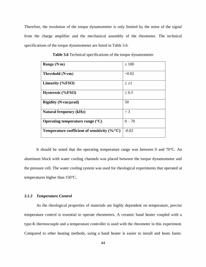
44
Therefore, the resolution of the torque dynamometer is only limited by the noise of the signal
from the charge amplifier and the mechanical assembly of the rheometer. The technical
specifications of the torque dynamometer are listed in Table 3.6.
Table 3.6 Technical specifications of the torque dynamometer
Range (N∙m) ± 100
Threshold (N∙cm) ~0.02
Linearity (%FSO) ≤ ±1
Hysteresis (%FSO) ≤ 0.5
Rigidity (N∙cm/𝜇rad) 50
Natural frequency (kHz) > 3
Operating temperature range (°C) 0 – 70
Temperature coefficient of sensitivity (%/°C) -0.02
It should be noted that the operating temperature range was between 0 and 70°C. An
aluminum block with water cooling channels was placed between the torque dynamometer and
the pressure cell. The water cooling system was used for rheological experiments that operated at
temperatures higher than 150°C.
3.1.3 Temperature Control
As the rheological properties of materials are highly dependent on temperature, precise
temperature control is essential to operate rheometers. A ceramic band heater coupled with a
type-K thermocouple and a temperature controller is used with the rheometer in this experiment.
Compared to other heating methods, using a band heater is easier to install and heats faster.
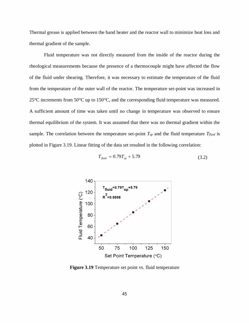
45
Thermal grease is applied between the band heater and the reactor wall to minimize heat loss and
thermal gradient of the sample.
Fluid temperature was not directly measured from the inside of the reactor during the
rheological measurements because the presence of a thermocouple might have affected the flow
of the fluid under shearing. Therefore, it was necessary to estimate the temperature of the fluid
from the temperature of the outer wall of the reactor. The temperature set-point was increased in
25°C increments from 50°C up to 150°C, and the corresponding fluid temperature was measured.
A sufficient amount of time was taken until no change in temperature was observed to ensure
thermal equilibrium of the system. It was assumed that there was no thermal gradient within the
sample. The correlation between the temperature set-point Tsp and the fluid temperature Tfluid is
plotted in Figure 3.19. Linear fitting of the data set resulted in the following correlation:
79.579.0 spfluid TT (3.2)
Figure 3.19 Temperature set point vs. fluid temperature

46
3.1.4 Motion Control and Data Acquisition
Another main component of the developed rheometer is a motor and motion controller. A
brushless DC motor was chosen in this study due to its advantages compared to a brushed DC
motor and a stepper motor: (1) smooth motion that minimizes system vibration and noise, (2)
excellent dynamic response, (3) higher speed, (4) higher torque than a comparably sized brushed
motor, and (5) a lower cost of maintenance. The technical specifications of the motor are listed in
Table 3.3. A quadrature encoder was assembled on the motor for keeping track of the position
and speed of the motor shaft. The resolution of the encoder was 20,000 PPR (pulses per
revolution), which corresponded to 0.018 degrees. The motor and encoder were connected to a
single-axis motion controller (DMC-31012, Galil), which controlled the motor using a closed
loop feedback. The motion controller had a built-in amplifier and communicated with a PC via
Ethernet.
Table 3.3 Technical specifications of the brushless DC motor
Rated voltage (V) 24
Rated power (W) 16
Rated speed (rpm) 1350
Rated torque (mN∙m) 110.0
Torque constant (mN∙m/A) 116.0
PID tuning parameters were determined to minimize the error between the commanded
and the actual motion profile. It should be noted that the tuning parameters were different
depending on the profile of motion and the load (friction and/or torque) acting on the shaft of the
motor. In certain conditions, the motion profile was highly sensitive to the tuning parameters and

47
did not follow the exact profile of the commanded motion. Therefore, the motion profile should
always be monitored to ensure whether it follows the commanded profile.
The motor controller also had many input and output ports for analog and digital signals
and a non-volatile memory that could record data in an array of up to 3000 elements (maximum
6 arrays) every 1 mins. Therefore, both the encoder and the torque signals could be recorded
without using a separate data acquisition board. Computer programs were developed using
LabVIEW for the motion control, monitoring/recording the analog and digital outputs, and
calculating the rheological parameters. The schematic diagram of the motion control and torque
measurement components and their connections are shown in Figure 3.20.
Figure 3.20 Elements of motion control and torque measurement
3.1.5 Bearing and Dynamic Seal
The rheometer utilizes a high temperature plastic ball bearing with stainless steel balls for
precise concentric rotational motion of the rotor with minimum friction. The dynamic seal used
48
to rotate the shaft is a PTFE lip seal with a stainless-steel U-spring. It has a continuous operating
pressure of 20.7 MPa and a temperature of 200°C, which are much higher values than the
operational range investigated in this study. The self-lubricating property of the seal allows for
use in dry conditions while maintaining pressure in the chamber even at rotational speeds up to
12,223 rpm (1,200 fpm). It should be noted that a slight leak occurred at the dynamic seal when
the vessel was pressurized. For this reason, gas was constantly fed into the vessel to maintain the
pressure. Further, there was a slight eccentricity due to the dimensional inaccuracy of the
machined parts and the bearing clearance.
A high pressure rotational rheometer was assembled using the components discussed
above. The function of the individual components along with their capabilities and limitations
are discussed in this section. In the following sections, the optimization and calibration of the
overall system is discussed.
3.2 Materials Studied
A certified Newtonian calibration fluid (Brookfield, #CAP8L) with a viscosity of 5,237
mPa∙s (at 25°C) was used in this study to calibrate the overall system and some preliminary
rheological measurements.
The investigated materials in this study are PDMS and CO2. The PDMS used in this
study is PSF-12500cSt from Clearco Products Co., Inc. It has a kinematic viscosity of 12,500 cSt
and a density of 0.97 g/cm3 at 25°C. From the silicone fluid equivalents chart provided by the
manufacturer and from information in an earlier study, PDMS is expected to have a molecular
weight (Mw) of 95,000 g/mol (Royer et al. 1999). CO2 with a purity of 99.9 % was purchased
from Praxair Co., Canada.

49
PDMS is chosen instead of heavy oil to avoid experimental difficulties and uncertainties
that can result from using heavy oil. Rheological measurements using heavy oil can be
significantly affected by the evaporation of lighter hydrocarbons, thermal degradation, phase
separation, etc. PDMS is the simplest silicone that has a silicone-oxygen-silicone backbone,
which is the basic structure of silicones. Another reason for choosing PDMS is for safety; it does
not produce any toxic gas and non-flammable. PDMS is a good model polymer melt to
investigate the gas plasticization of polymer melts due to its high gas solubility mostly with CO2.
The low melting temperature of PDMS eliminates the experimental difficulty of melting
engineering thermoplastics.
3.3 Gap Optimization
In concentric cylinder geometry, it is assumed that torque induced on the outer cylinder is
mostly due to the shearing of the fluid between the inner and outer cylinder. However, there is an
extra torque contribution due to the shearing of the fluid between the bottoms of the cylinders,
which is commonly referred to as “end effect.” This effect is one of the major sources of error in
concentric cylinder rheometers and should be minimized or corrected. In this section, the effect
of the bottom plate gap is evaluated using the Newtonian calibration fluid at various gap
distances. The gap distance that is used for the subsequent rheological measurement is
determined based on the result.
The torque of flow at the bottom of the cylinder can be approximated as a flow between
parallel plates. The extra torque contribution at the bottom of the cylinder can be estimated using
the following equation:
50
h
RM i
p2
4
(3.3)
where Ri is the radius of the inner cylinder, 𝜂 is the viscosity of a Newtonian fluid, Ω is the
angular velocity, and h is the distance between the plates. The torque contribution at the wall of
cylinder can be expressed as follows:
2)/(1
4
oi
o
cRR
LRM
(3.4)
where Ro is the radius of the outer cylinder, L is the length of the cylinder. Therefore, the total
torque can be expressed as the sum of these two contributions:
pctot MMM (3.5)
Figure 3.21 shows the theoretical estimation and experimental measurement of the total
torque as a function of the gap spacing at the bottoms of the cylinders at various angular
velocities using the calibration fluid. Since Mp is inversely proportional to h, the torque
contribution at the end of the cylinder could be negligible if h is large enough compared to the
gap between the concentric cylinders (Ro − Ri). According to the theoretical calculation, the
torque contribution due to the end effect at a 3.2 mm gap was only 5.4 % of Mc. Experimentally,
a parallel gap larger than 3.2 mm has a negligible contribution on the total torque measurement.
Therefore, the gap spacing was fixed at 3.2 mm for all experiments conducted in this study.

51
Figure 3.21 Theoretical estimation compared with experimental data of the total torque values
versus the distance of the parallel gap
3.4 Rheometer Calibration
The calibration of the overall system includes compensation for system friction and the
evaluation of the calibration coefficient. The methods used for the friction compensation are
discussed along with their limitations. Then, the calibration coefficient is determined using a
calibration fluid with known viscosity.
3.4.1 Friction Compensation
The developed rheometer utilizes a high pressure dynamic seal, which produces
additional torque due to the friction between the seal and the shaft. This torque is quite high
compared to the torque caused by the shearing of the test fluid. Therefore, the torque
measurement should be compensated for the friction. The measured torque Mmeasured is the sum of
the two contributions:

52
frictionfluidmeasured MMM (3.6)
where Mfluid is the torque cause by the shearing of the fluid, and Mfriction is the torque caused by
the friction between the seal and the shaft. The torque caused by the seal friction should be
subtracted from the measured torque to obtain the torque caused by the shearing of the fluid.
The seal friction under steady shear mode was evaluated by rotating the rheometer
without any liquid at various rotational speeds and measuring the resulting torque. All
measurements were repeated three times. Shear rates were calculated using the angular speed and
geometry of the concentric cylinder:
2
1
2
o
i
R
R
(3.7)
The torque values measured while the empty rheometer was rotated at various shear rates are
shown in Figure 3.22. The torque was 0.093 N∙m at 15.6 s-1; it increased to 0.116 N∙m as the
shear rate increased. These values are significant considering the torque exerted on the fluid (the
maximum torque that the motor can produce is approximately 0.25 N∙m). The large friction
value can result in a large measurement scatter, especially at lower shear rates.
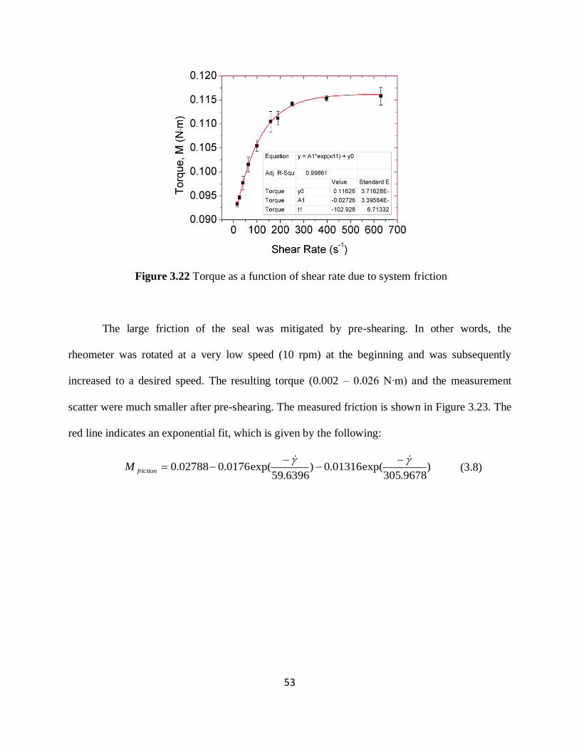
53
Figure 3.22 Torque as a function of shear rate due to system friction
The large friction of the seal was mitigated by pre-shearing. In other words, the
rheometer was rotated at a very low speed (10 rpm) at the beginning and was subsequently
increased to a desired speed. The resulting torque (0.002 – 0.026 N∙m) and the measurement
scatter were much smaller after pre-shearing. The measured friction is shown in Figure 3.23. The
red line indicates an exponential fit, which is given by the following:
)9678.305
exp(01316.0)6396.59
exp(0176.002788.0
frictionM (3.8)

54
Figure 3.23 Torque as a function of shear rate due to system friction
If a fluid is measured in the same manner (pre-shearing) and the torque given by the above
equation is subtracted from the total torque, the torque from the shearing of the fluid can be
easily determined. However, the torque (or shear stress) curve does not pass through the origin
anymore because the torque contribution is missing between 0 – 10 rpm (Figure 3.24). This issue
could be corrected by vertically shifting the curve so that the curve passes through the origin,
assuming that the torque and shear rate is linear between 0 – 10 rpm. This approach is reasonable
because many fluids, including polymeric liquids, have a Newtonian plateau region where the
shear stress and the shear rate have a linear relationship at low shear rates. Since PDMS also has
a distinctive Newtonian plateau, it is not problematic to correct the torque and to get reliable,
steady shear results. However, some fluids that have non-linearity at low shear rates or yield
stress cannot be corrected in this way.
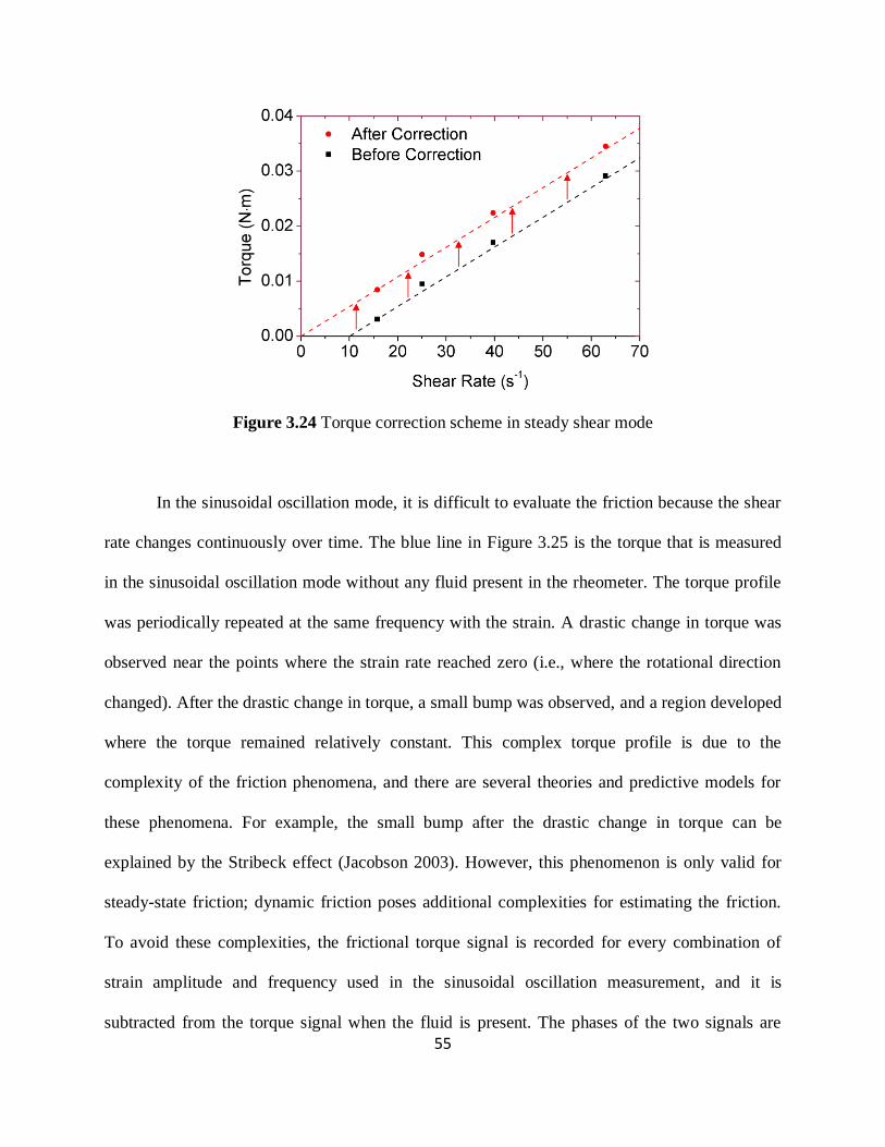
55
Figure 3.24 Torque correction scheme in steady shear mode
In the sinusoidal oscillation mode, it is difficult to evaluate the friction because the shear
rate changes continuously over time. The blue line in Figure 3.25 is the torque that is measured
in the sinusoidal oscillation mode without any fluid present in the rheometer. The torque profile
was periodically repeated at the same frequency with the strain. A drastic change in torque was
observed near the points where the strain rate reached zero (i.e., where the rotational direction
changed). After the drastic change in torque, a small bump was observed, and a region developed
where the torque remained relatively constant. This complex torque profile is due to the
complexity of the friction phenomena, and there are several theories and predictive models for
these phenomena. For example, the small bump after the drastic change in torque can be
explained by the Stribeck effect (Jacobson 2003). However, this phenomenon is only valid for
steady-state friction; dynamic friction poses additional complexities for estimating the friction.
To avoid these complexities, the frictional torque signal is recorded for every combination of
strain amplitude and frequency used in the sinusoidal oscillation measurement, and it is
subtracted from the torque signal when the fluid is present. The phases of the two signals are
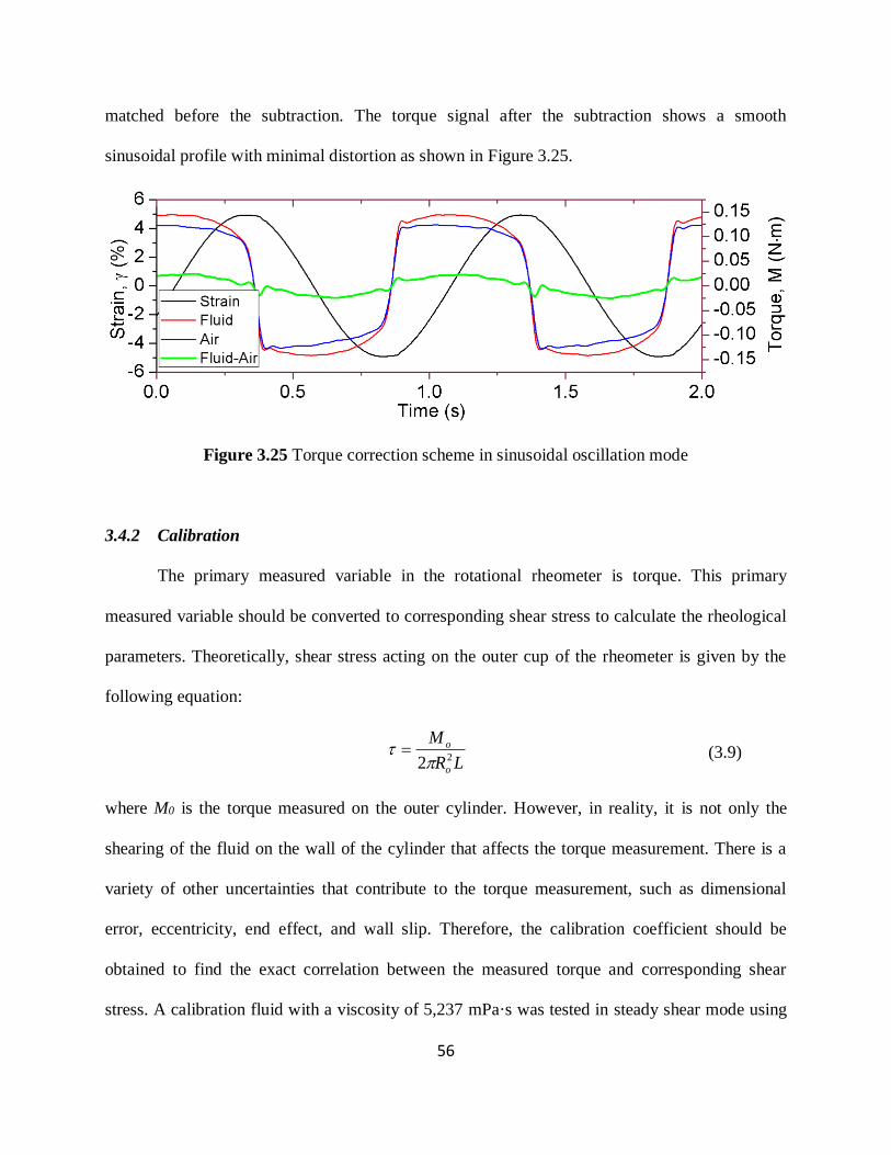
56
matched before the subtraction. The torque signal after the subtraction shows a smooth
sinusoidal profile with minimal distortion as shown in Figure 3.25.
Figure 3.25 Torque correction scheme in sinusoidal oscillation mode
3.4.2 Calibration
The primary measured variable in the rotational rheometer is torque. This primary
measured variable should be converted to corresponding shear stress to calculate the rheological
parameters. Theoretically, shear stress acting on the outer cup of the rheometer is given by the
following equation:
LR
M
o
o
22 (3.9)
where M0 is the torque measured on the outer cylinder. However, in reality, it is not only the
shearing of the fluid on the wall of the cylinder that affects the torque measurement. There is a
variety of other uncertainties that contribute to the torque measurement, such as dimensional
error, eccentricity, end effect, and wall slip. Therefore, the calibration coefficient should be
obtained to find the exact correlation between the measured torque and corresponding shear
stress. A calibration fluid with a viscosity of 5,237 mPa·s was tested in steady shear mode using
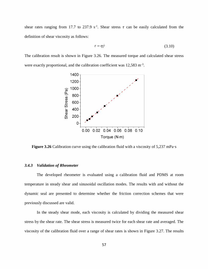
57
shear rates ranging from 17.7 to 237.9 s-1. Shear stress 𝜏 can be easily calculated from the
definition of shear viscosity as follows:
(3.10)
The calibration result is shown in Figure 3.26. The measured torque and calculated shear stress
were exactly proportional, and the calibration coefficient was 12,583 m-3.
Figure 3.26 Calibration curve using the calibration fluid with a viscosity of 5,237 mPa·s
3.4.3 Validation of Rheometer
The developed rheometer is evaluated using a calibration fluid and PDMS at room
temperature in steady shear and sinusoidal oscillation modes. The results with and without the
dynamic seal are presented to determine whether the friction correction schemes that were
previously discussed are valid.
In the steady shear mode, each viscosity is calculated by dividing the measured shear
stress by the shear rate. The shear stress is measured twice for each shear rate and averaged. The
viscosity of the calibration fluid over a range of shear rates is shown in Figure 3.27. The results
58
show that the viscosity when the dynamic seal is used resulted in a much closer value to the
actual viscosity of the calibration fluid (5,237 mPa∙s) than when the dynamic seal was not used.
The viscosity was also relatively constant over the investigated shear rate range, which was
expected for the Newtonian fluid. Without the seal, the viscosity was slightly overestimated at
lower shear rates (~6,000 mPa∙s), and it approached a value close to the actual viscosity at higher
shear rates. The steady shear results for PDMS are shown in Figure 3.28 . Since PDMS is a
typical shear-thinning fluid, it is expected that the viscosity is constant at lower shear rates
(Newtonian plateau region) and that it decreases at higher shear rates (power-law region).
Although the viscosity of the PDMS is unknown, viscosity in the Newtonian plateau region can
be approximated by dividing the kinematic viscosity (12,500 cSt) by the density (0.975 at 25°C),
which results in 12,821 mPa∙s. Similar to the case of the calibration fluid, with the seal, the
viscosity was much closer to the value of the actual viscosity compared to the case when no seal
was used; therefore, without the seal, in this case the viscosity was underestimated. PDMS did
not show distinctive shear-thinning behavior within the range of the investigated shear rates.
From the above observations, the steady shear measurement with the seal gives a reasonably
accurate viscosity value. This result demonstrates that the torque correction scheme discussed in
the previous section is valid.
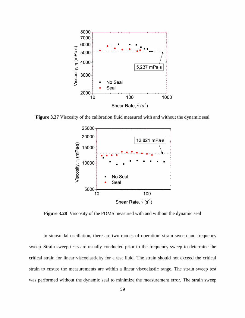
59
Figure 3.27 Viscosity of the calibration fluid measured with and without the dynamic seal
Figure 3.28 Viscosity of the PDMS measured with and without the dynamic seal
In sinusoidal oscillation, there are two modes of operation: strain sweep and frequency
sweep. Strain sweep tests are usually conducted prior to the frequency sweep to determine the
critical strain for linear viscoelasticity for a test fluid. The strain should not exceed the critical
strain to ensure the measurements are within a linear viscoelastic range. The strain sweep test
was performed without the dynamic seal to minimize the measurement error. The strain sweep
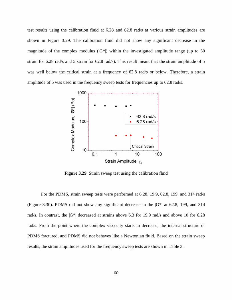
60
test results using the calibration fluid at 6.28 and 62.8 rad/s at various strain amplitudes are
shown in Figure 3.29. The calibration fluid did not show any significant decrease in the
magnitude of the complex modulus (|G*|) within the investigated amplitude range (up to 50
strain for 6.28 rad/s and 5 strain for 62.8 rad/s). This result meant that the strain amplitude of 5
was well below the critical strain at a frequency of 62.8 rad/s or below. Therefore, a strain
amplitude of 5 was used in the frequency sweep tests for frequencies up to 62.8 rad/s.
Figure 3.29 Strain sweep test using the calibration fluid
For the PDMS, strain sweep tests were performed at 6.28, 19.9, 62.8, 199, and 314 rad/s
(Figure 3.30). PDMS did not show any significant decrease in the |G*| at 62.8, 199, and 314
rad/s. In contrast, the |G*| decreased at strains above 6.3 for 19.9 rad/s and above 10 for 6.28
rad/s. From the point where the complex viscosity starts to decrease, the internal structure of
PDMS fractured, and PDMS did not behaves like a Newtonian fluid. Based on the strain sweep
results, the strain amplitudes used for the frequency sweep tests are shown in Table 3..
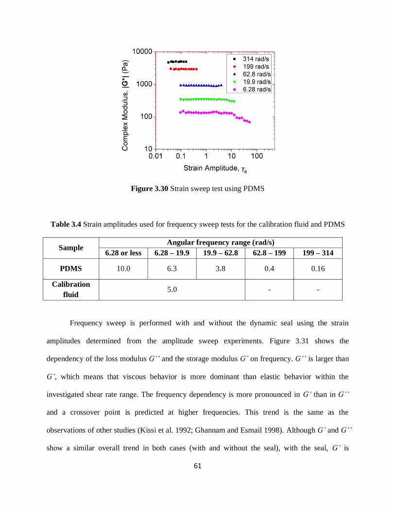
61
Figure 3.30 Strain sweep test using PDMS
Table 3.4 Strain amplitudes used for frequency sweep tests for the calibration fluid and PDMS
Sample Angular frequency range (rad/s)
6.28 or less 6.28 – 19.9 19.9 – 62.8 62.8 – 199 199 – 314
PDMS 10.0 6.3 3.8 0.4 0.16
Calibration
fluid 5.0 - -
Frequency sweep is performed with and without the dynamic seal using the strain
amplitudes determined from the amplitude sweep experiments. Figure 3.31 shows the
dependency of the loss modulus G’’ and the storage modulus G’ on frequency. G’’ is larger than
G’, which means that viscous behavior is more dominant than elastic behavior within the
investigated shear rate range. The frequency dependency is more pronounced in G’ than in G’’
and a crossover point is predicted at higher frequencies. This trend is the same as the
observations of other studies (Kissi et al. 1992; Ghannam and Esmail 1998). Although G’ and G’’
show a similar overall trend in both cases (with and without the seal), with the seal, G’ is
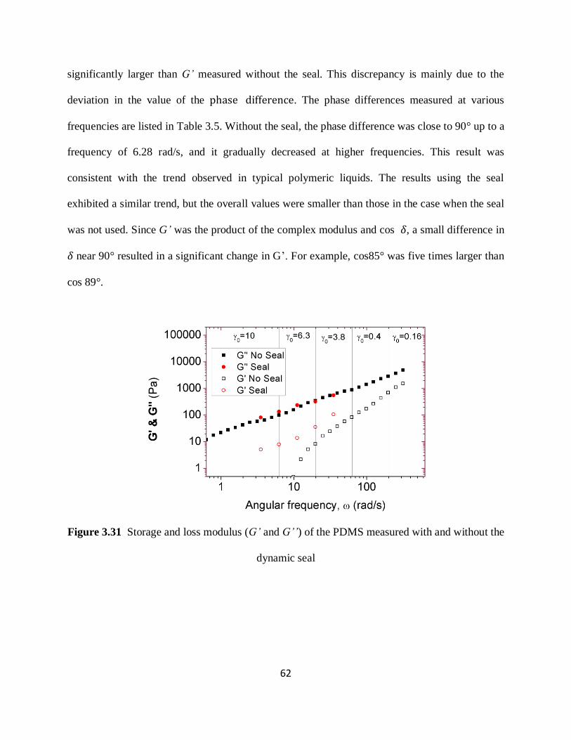
62
significantly larger than G’ measured without the seal. This discrepancy is mainly due to the
deviation in the value of the phase difference. The phase differences measured at various
frequencies are listed in Table 3.5. Without the seal, the phase difference was close to 90° up to a
frequency of 6.28 rad/s, and it gradually decreased at higher frequencies. This result was
consistent with the trend observed in typical polymeric liquids. The results using the seal
exhibited a similar trend, but the overall values were smaller than those in the case when the seal
was not used. Since G’ was the product of the complex modulus and cos 𝛿, a small difference in
𝛿 near 90° resulted in a significant change in G’. For example, cos85° was five times larger than
cos 89°.
Figure 3.31 Storage and loss modulus (G’ and G’’) of the PDMS measured with and without the
dynamic seal
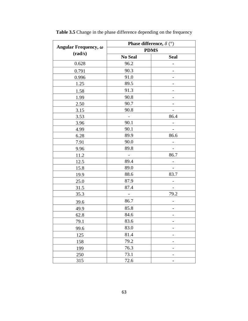
63
Table 3.5 Change in the phase difference depending on the frequency
Angular Frequency, 𝜔
(rad/s)
Phase difference, 𝛿 (°)
PDMS
No Seal Seal
0.628 96.2 -
0.791 90.3 -
0.996 91.0 -
1.25 89.5 -
1.58 91.3 -
1.99 90.8 -
2.50 90.7 -
3.15 90.8 -
3.53 - 86.4
3.96 90.1 -
4.99 90.1 -
6.28 89.9 86.6
7.91 90.0 -
9.96 89.8 -
11.2 - 86.7
12.5 89.4 -
15.8 89.0 -
19.9 88.6 83.7
25.0 87.9 -
31.5 87.4 -
35.3 - 79.2
39.6 86.7 -
49.9 85.8 -
62.8 84.6 -
79.1 83.6 -
99.6 83.0 -
125 81.4 -
158 79.2 -
199 76.3 -
250 73.1 -
315 72.6 -

64
There are several possible reasons for this deviation. First, the strain profile is not a
complete sinusoidal profile due to the excessive friction of the seal. There is always some
distortion, especially at the peak strain (where the rotational direction changes). Second, the
frictional torque measured without any liquid cannot exactly match the frictional torque when a
fluid is present. Nevertheless, the results when the seal was used can provide reliable information
in terms of the relative change in the viscoelasticity of a fluid.
The magnitude of the complex viscosity |𝜂*| is shown in Figure 3.32. The |𝜂*| is
distributed between 14,000 and 22,000 mPa∙s without showing any consistent trend. In fact, it is
widely accepted that the complex viscosity has a close relationship with the shear viscosity 𝜂:
)(|)(*| with (3.11)
where 𝜔 is angular frequency. This empirical relationship is called the “Cox-Merz rule” (Cox
and Merz 1958) and has been found to be true for most of the polymer melts. Therefore, the
deviation of |𝜂*| from the value of the steady shear viscosity 𝜂 (12,821 mPa∙s) can be regarded as
a measurement error.
Figure 3.32 Magnitude of the complex viscosity (|𝜂*|) of the PDMS measured with and without
the dynamic seal
65
3.5 Summary
The overall design and some major components of the developed rheometer were
presented in this chapter. One of the main characteristics of the developed rheometer was the use
of the piezoelectric torque dynamometer. The piezoelectric torque dynamometer had exceptional
linearity over a wide range of torque values, superiority in dynamic measurements, and was less
dependent on temperature. The developed rheometer also utilized the dynamic shaft seal, which
allowed for rheological measurements under high pressure. The torque dynamometer was
calibrated to determine the transducer sensitivity and scale factor for a charge amplifier. The
temperature control, motion control, data acquisition, and bearing/shaft seal were also described
in detail. The effect of the distance between the cylinder bottoms on the torque measurement was
investigated to find the minimum distance where the end effect was negligible. The rheometer
was then calibrated using the calibration fluid with known viscosity to find the correlation
between torque and shear stress. The friction correction schemes for each modes of operation
were also presented.
The operation of the developed rheometer was validated using the calibration fluid and
PDMS in each mode of operation at room temperature. The rheological measurements were
conducted with and without the dynamic seal to validate the effectiveness of the friction
correction schemes. In the steady shear mode, using the dynamic seal and the correction scheme
resulted in accurate viscosity measurements. In the sinusoidal oscillation mode, it was
demonstrated that G’, G’’, and |𝜂*| could be measured between 0.628 and 315 rad/s (without the
seal) and 3.52 and 35.2 rad/s (with the seal).
66
CHAPTER 4: EXPERIMENTAL RESULTS AND MODELING
In this chapter, the effects of temperature and dissolved CO2 on the rheological properties
of PDMS are investigated using the developed rheometer in both steady shear and sinusoidal
oscillation mode. The effects of the individual parameters on the viscosity are experimentally
investigated and correlated using several models. The prediction of the amount of dissolved CO2
at a given temperature and pressure is also presented. Then, empirical models are proposed that
account for the combined effect of temperature and pressure on the viscosity. One of the main
advantage of the proposed models is that the viscosity can be predicted at a given temperature
and pressure without knowing the volumetric properties of the pure components and the mixture.
In addition to the viscosity measurement, the dynamic rheological parameters are also measured
at various temperatures and CO2 saturation pressures. The capability and the limitations of the
developed system are also discussed.
4.1 Steady Shear Measurement
4.1.1 Effects of Temperature
Steady shear measurements were conducted using PDMS at various shear rates and
temperatures at 25°C, 50°C, and 80°C. Sufficient time was allowed before measuring for the
system to be in the thermal equilibrium state. The results are shown in Figure 3.17. It was
observed that the viscosity of the PDMS was highly sensitive to temperature variations. It was
also observed that the PDMS exhibited the behavior of a Newtonian fluid within the temperature
and shear rate range investigated. The viscosity data at a lower shear rate range was ignored
because there was a noticeable deviation from the Newtonian behavior. At lower shear rates, the
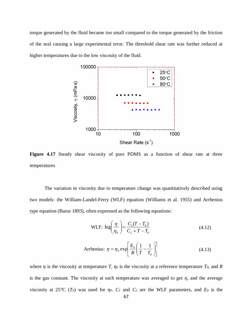
67
torque generated by the fluid became too small compared to the torque generated by the friction
of the seal causing a large experimental error. The threshold shear rate was further reduced at
higher temperatures due to the low viscosity of the fluid.
Figure 4.17 Steady shear viscosity of pure PDMS as a function of shear rate at three
temperatures
The variation in viscosity due to temperature change was quantitatively described using
two models: the William-Landel-Ferry (WLF) equation (Williams et al. 1955) and Arrhenius
type equation (Barus 1893), often expressed as the following equations:
WLF: 02
01
0
)(log
TTC
TTC
(4.12)
Arrhenius:
0
0
0
11exp
TTR
E (4.13)
where 𝜂 is the viscosity at temperature T, 𝜂0 is the viscosity at a reference temperature T0, and R
is the gas constant. The viscosity at each temperature was averaged to get 𝜂, and the average
viscosity at 25°C (T0) was used for 𝜂0. C1 and C2 are the WLF parameters, and E0 is the
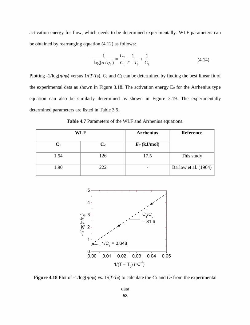
68
activation energy for flow, which needs to be determined experimentally. WLF parameters can
be obtained by rearranging equation (4.12) as follows:
101
2
0
11
)/log(
1
CTTC
C
(4.14)
Plotting -1/log(𝜂/𝜂0) versus 1/(T-T0), C1 and C2 can be determined by finding the best linear fit of
the experimental data as shown in Figure 3.18. The activation energy E0 for the Arrhenius type
equation can also be similarly determined as shown in Figure 3.19. The experimentally
determined parameters are listed in Table 3.5.
Table 4.7 Parameters of the WLF and Arrhenius equations.
WLF Arrhenius Reference
C1 C2 E0 (kJ/mol)
1.54 126 17.5 This study
1.90 222 - Barlow et al. (1964)
Figure 4.18 Plot of -1/log(𝜂/𝜂0) vs. 1/(T-T0) to calculate the C1 and C2 from the experimental
data

69
Figure 4.19 Plot of -ln(𝜂/𝜂0) vs. 1/R (T0-T) to calculate the E0 from the experimental data
The experimentally measured viscosity along with the fitted lines for the two models are
depicted in Figure 3.20. Viscosity of PDMS was reduced by 44.4% at 50°C and 65.9% at 80°C
compared to the viscosity at the reference temperature. Both models showed excellent agreement
with the experimental data while the WLF correlation provided a slightly better fit to the
experimental data.
Figure 4.20 Viscosity of pure PDMS at various temperature with best-fit WLF and Arrhenius
correlations. The reference temperature, T0, is 25°C.

70
4.1.2 Effects of Dissolved CO2
High pressure measurements were performed in the steady shear mode to evaluate the
effect of dissolved CO2 on the viscosity of the PDMS. The rheometer was first purged with CO2
for 10 minutes to replace air in the pressure cell to CO2 and then pressurized using a high
pressure regulator to a desired pressure. The viscosity was periodically monitored during the
dissolution process until no further viscosity reduction is observed to ensure the complete
saturation of the CO2 in the PDMS.
Viscosities of the PDMS-CO2 at various shear rates at temperature of 50°C and pressure
up to 3 MPa are shown in Figure 4.21. It was observed that the viscosity of the PDMS is highly
sensitive to the pressure variation similar to that was observed for temperature variation. It was
also observed that the PDMS exhibits behavior of Newtonian fluid within the pressure and shear
rate range investigated. It should be noted that the maximum shear rate is significantly reduced at
the higher pressures. This is due to the increased friction at the dynamic seal at higher pressures,
thus causing the motor torque limit is reached at much lower shear rates. The dashed line
indicates the minimum viscosity that can be measured accurately at given shear rates which
corresponds to the torque of 20 mN∙m. Viscosity data below this line showed large experimental
scatter. The measurement fluctuation within the measurement range was about ±5%.
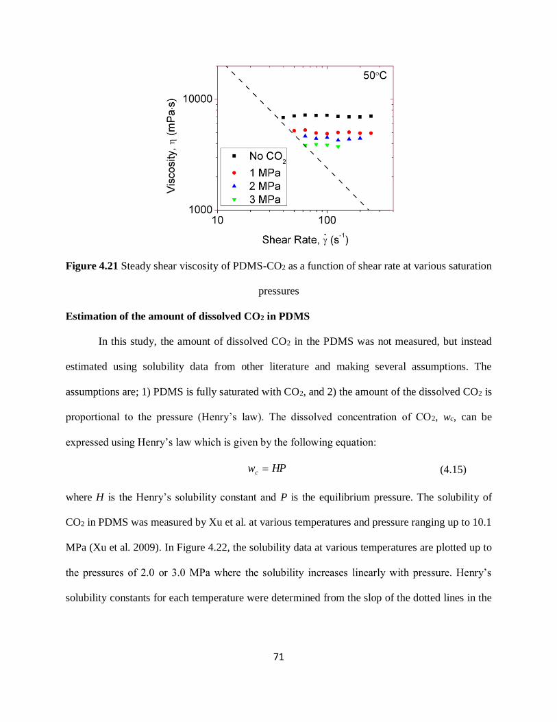
71
Figure 4.21 Steady shear viscosity of PDMS-CO2 as a function of shear rate at various saturation
pressures
Estimation of the amount of dissolved CO2 in PDMS
In this study, the amount of dissolved CO2 in the PDMS was not measured, but instead
estimated using solubility data from other literature and making several assumptions. The
assumptions are; 1) PDMS is fully saturated with CO2, and 2) the amount of the dissolved CO2 is
proportional to the pressure (Henry’s law). The dissolved concentration of CO2, wc, can be
expressed using Henry’s law which is given by the following equation:
HPwc (4.15)
where H is the Henry’s solubility constant and P is the equilibrium pressure. The solubility of
CO2 in PDMS was measured by Xu et al. at various temperatures and pressure ranging up to 10.1
MPa (Xu et al. 2009). In Figure 4.22, the solubility data at various temperatures are plotted up to
the pressures of 2.0 or 3.0 MPa where the solubility increases linearly with pressure. Henry’s
solubility constants for each temperature were determined from the slop of the dotted lines in the

72
plot and they are listed in Table 3.6. The temperature dependency of the Henry’s solubility
constant is generally expressed in the following form (Smith and Harvey 2007):
0
0
11exp)(
TTR
EHTH s
(4.16)
where T0 is the reference temperature (35°C in this case), H0 is the Henry’s constant at T0, and Es
is the enthalpy of dissolution. Es can be determined by plotting ln(𝐻/𝐻0) versus 1/𝑅(1/𝑇 −
1/𝑇0) as shown in Figure 4.23 (Es = -11.8).
Figure 4.22 Equilibrium solubility of CO2 in PDMS at various temperatures (Xu et al. 2009)
Table 4.8 Henry’s solubility constant at various temperatures
Temperature (°C) 35 40 50 80 100
H (MPa-1) 2.56E-2 2.32E-2 1.92E-2 1.42E-2 1.12E-2

73
Figure 4.23 Plot of ln(H/H0) vs. 1/R (1/T-1/T0) to calculate the Es from the experimental data
By substituting the equation (4.16) into equation (4.15) and using the determined
parameters, weight fraction of CO2 in the PDMS at a given temperature and pressure can be
predicted using the following equation:
PT
PTwc
15.308
111041.1exp0256.0),( 3
(4.17)
Effect of dissolved CO2 on the viscosity of PDMS
Using the above equation, the weight fractions of CO2 under the experimental conditions
were calculated. The average viscosity as a function of weight fraction of CO2 is shown in Figure
3.21 along with several models. One of the models is a simple exponential equation proposed by
Yeo and Kiran (1999) which is given by:
)exp(,0 cw Bwc
(4.18)
74
wherecw,0 is the viscosity of the pure polymer and B is a constant. This model showed noticeable
deviation from the experimental results. The poor agreement led us to add a second order term in
the exponent:
)exp(2
,0 ccw CwBwc
(4.19)
where the C is also a constant. Although this model provided a better fit to the experimental data,
there is no physical significance in B and C. Another model considered in this study is the
equation proposed by Fujita and Kishimoto (1958) which is given by:
c
c
w wf
wf
c
/
)/1(ln
,0
(4.20)
where f is the fractional free volume and 𝜃 is the parameter representing the contribution of the
dissolved gas in increasing the free volume. In this study, the f and 𝜃 are considered as adjustable
parameters. Rearranging equation (4.20) yields:
fw
f
cwc
1
)/ln(
1 2
,0 (4.10)
f and 𝜃 can be obtained by plotting 1/ln(𝜂/cw,0 ) versus 1/wc as shown in Figure 3.26. The Fujita-
Kishimoto equation showed good agreement with the experimental data. The model parameters
determined for each predictive model are presented in Table 3..

75
Figure 4.24 Viscosity of PDMS at various weight fraction of CO2 and 50°C along with several
predictive models.
Figure 4.25 Plot of 1/ln(𝜂/cw,0 ) vs 1/wc as to calculate the f and 𝜃 from the experimental data
Table 4.9 Parameters of the models that account for the CO2 concentration
Yeo and Kiran Exponential w/ 2nd order polynomial Fujita-Kishimoto
B B C f 𝜃
-10.9 -17.2 122 1.11 32.8

76
Figure 3.22 shows the relative change of the viscosity of the PDMS as a function of
weight fraction of CO2 at 50°C. The data of Gerhardt et al. (1997) obtained using a capillary
extrusion rheometer is also presented for comparison. Both data show reasonable agreement thus
confirming the validity the developed rheometer. Small deviations between the two study can be
attributed to the different molecular weight of the PDMS. Gerhardt et al. used higher molecular
weight PDMS (Mw=308,000 g/mol) in comparison with this study (Mw=95,000 g/mol).
Figure 4.26 Effect of the weight fraction of CO2 on relative viscosity of PDMS
4.2 Modeling
The combined effects of temperature and pressure on the viscosity of the PDMS-CO2
system were investigated. Although there have been numerous attempts to predict viscosity of
polymer-gas system, most of the proposed models require volumetric parameters (e.g. specific
volume and occupied volume) of the individual components and the mixture which are difficult
to measure. Prediction of these volumetric parameters is also challenging because of the complex
thermodynamic concept involved and requires physical and thermodynamic properties of the
materials. Therefore, these approaches are lack of practical significance and cannot be readily

77
used for predicting viscosity at certain processing conditions. In order to avoid the difficulties, a
viscosity prediction model based on empirical approach was developed. It will be shown that the
viscosity of the PDMS-CO2 can be expressed as a function of temperature and pressure.
Viscosity of polymer-gas system has been expressed mathematically in terms of
temperature (T), pressure (P), and weight fraction of dissolved gas (wc) using the following form
which is known as generalized Arrhenius equation (Lee et al. 1999; Ladin et al. 2001):
)(exp),,( termsorderhigherwP
TTAwPT c
r
c
(4.21)
where A, 𝛼, Tr, 𝛽, and 𝜓 are constants. By dropping the higher order terms and the pressure term
(assuming that the pressure has negligible effect on the viscosity), equation (4.21) becomes:
c
r
c wTT
AwT
exp),(
(4.22)
Equation (4.22) can be further modified by replacing the temperature related term with the
Arrhenius type equation (4.13) because they both are in exponential form:
cc w
TTR
EAwT
0
0 11exp),(
(4.23)
The empirical constants A, 𝛼, Tr, E0, and 𝜓 were determined using a least-square method based
on the Trust-Region algorithm. Using this algorithm, the constants were successfully determined
as shown in Table 4.10.
Table 4.10 Parameters of the models of the temperature and the gas concentration dependency
Generalized Arrhenius model Modified generalized Arrhenius model
A Tr 𝛼 𝜓 A E0 𝜓
593 -76.5 311 -11.6 1.26E4 18.3 -12.2

78
By substitute equation (4.17) into the both models, viscosity can be expressed as a
function of temperature and pressure. The experimentally measured viscosity and the predicted
viscosity using the two models are shown in Figure 3.23 and Figure 3.24. Both models showed
good agreement with the experimental data and they could describe the effect of the temperature
and CO2 saturation pressure on the viscosity of PDMS-CO2.
Figure 4.27 Viscosity as a function of temperature and pressure predicted using the generalized
Arrhenius equation
Figure 4.28 Viscosity as a function of temperature and pressure predicted using the modified
generalized Arrhenius equation
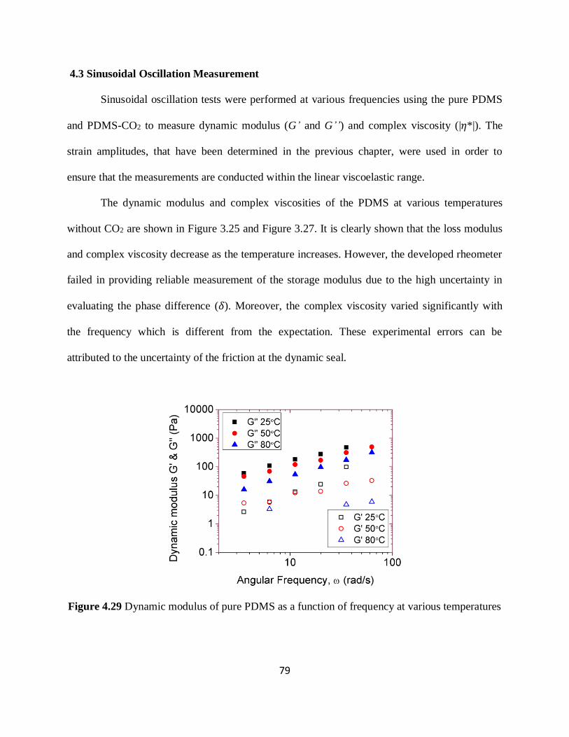
79
4.3 Sinusoidal Oscillation Measurement
Sinusoidal oscillation tests were performed at various frequencies using the pure PDMS
and PDMS-CO2 to measure dynamic modulus (G’ and G’’) and complex viscosity (|𝜂*|). The
strain amplitudes, that have been determined in the previous chapter, were used in order to
ensure that the measurements are conducted within the linear viscoelastic range.
The dynamic modulus and complex viscosities of the PDMS at various temperatures
without CO2 are shown in Figure 3.25 and Figure 3.27. It is clearly shown that the loss modulus
and complex viscosity decrease as the temperature increases. However, the developed rheometer
failed in providing reliable measurement of the storage modulus due to the high uncertainty in
evaluating the phase difference (𝛿). Moreover, the complex viscosity varied significantly with
the frequency which is different from the expectation. These experimental errors can be
attributed to the uncertainty of the friction at the dynamic seal.
Figure 4.29 Dynamic modulus of pure PDMS as a function of frequency at various temperatures
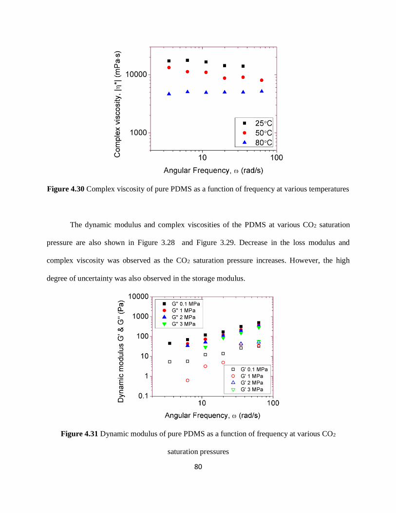
80
Figure 4.30 Complex viscosity of pure PDMS as a function of frequency at various temperatures
The dynamic modulus and complex viscosities of the PDMS at various CO2 saturation
pressure are also shown in Figure 3.28 and Figure 3.29. Decrease in the loss modulus and
complex viscosity was observed as the CO2 saturation pressure increases. However, the high
degree of uncertainty was also observed in the storage modulus.
Figure 4.31 Dynamic modulus of pure PDMS as a function of frequency at various CO2
saturation pressures

81
Figure 4.32 Complex viscosity of pure PDMS as a function of frequency at various CO2
saturation pressures
Overall, the developed rheometer could give information on how the dynamic rheological
parameters are changed at various temperature and CO2 saturation pressure in general. It was
shown that the increase of temperature and saturation pressure resulted in decreased loss
modulus and complex viscosity. However, the change of the storage modulus could be not
clearly distinguished due to the experimental error.
4.4 Summary
This chapter presented the effects of temperature, pressure, and dissolved CO2 on the
rheological parameters of the PDMS. Viscosities of PDMS at various temperature and CO2
saturation pressure were successfully measured using the developed rheometer. The temperature
dependency was found to fit both WLF and Arrhenius equation. The amount of dissolved CO2 at
the corresponding pressure and temperature was estimated using Henry’s law. The Fujita-
Kishimoto equation and the exponential equation whose exponent contains the second order
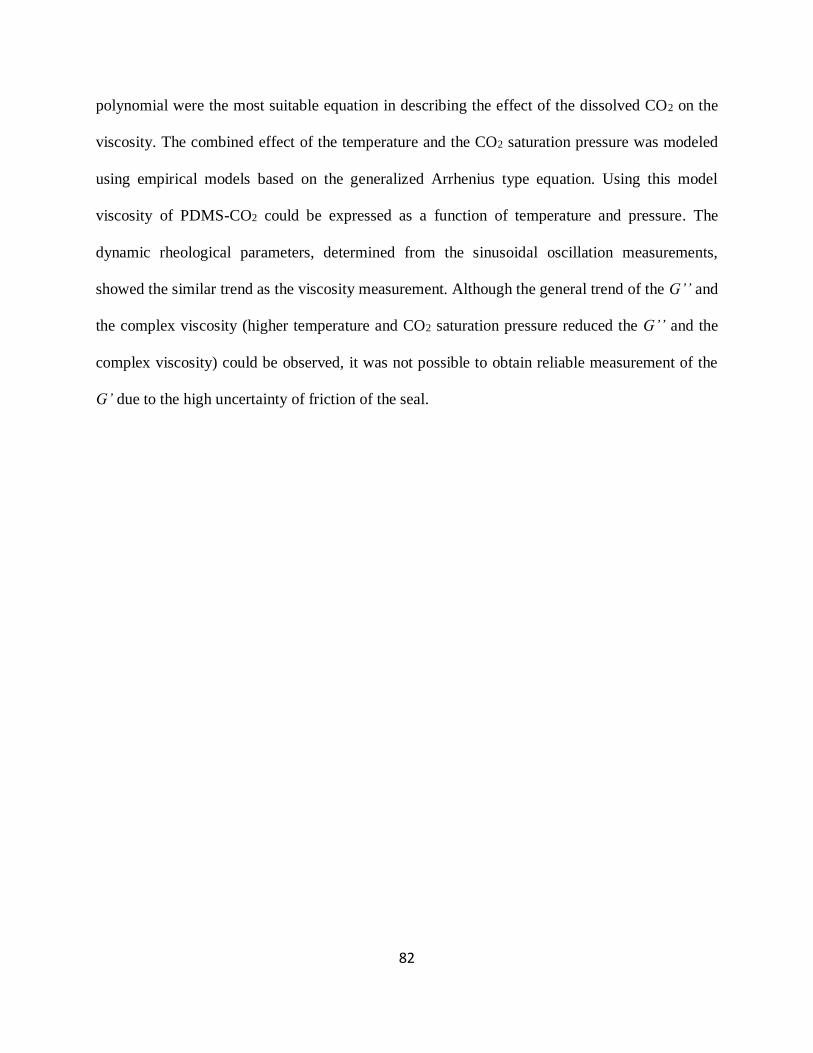
82
polynomial were the most suitable equation in describing the effect of the dissolved CO2 on the
viscosity. The combined effect of the temperature and the CO2 saturation pressure was modeled
using empirical models based on the generalized Arrhenius type equation. Using this model
viscosity of PDMS-CO2 could be expressed as a function of temperature and pressure. The
dynamic rheological parameters, determined from the sinusoidal oscillation measurements,
showed the similar trend as the viscosity measurement. Although the general trend of the G’’ and
the complex viscosity (higher temperature and CO2 saturation pressure reduced the G’’ and the
complex viscosity) could be observed, it was not possible to obtain reliable measurement of the
G’ due to the high uncertainty of friction of the seal.
83
CHAPTER 5: CONCLUSION
Understanding the rheological properties of materials under high pressure is important
because various industrial processes operate under high pressure. However, many studies on the
high pressure rheology have been relied on pressure-driven rheometers or falling ball rheometers
that have limited capability in term of performing various rheological measurement. Several
studies have developed high pressure rotational rheometers, but they have limited capability in
dynamic rheological measurement due to the inertia and compliance of the torque transducer
they used. In this thesis, a concentric cylinder rheometer was developed that was designed to
perform high pressure rheological measurements. Effects of temperature and pressure on the
rheological properties of PDMS-CO2 system were investigated using the developed rheometer.
In this chapter, a summary and the novel contributions of the presented work are provided.
Furthermore, the assumptions and limitations of the experiments and modeling are discussed
followed by suggestions for possible future work.
5.1 Summary
In this thesis, a high pressure rotational was designed, fabricated, and calibrated for
taking rheological measurements of viscoelastic fluids. The concentric cylinder was adopted to
minimize errors associated with the fluid volume swelling, which was caused by dissolving gas
in the fluids under high pressure. The closed chamber design of the concentric cylinder and using
a dynamic seal for the shaft of the inner cylinder enabled the pressurization of gas up to 3 MPa.
The inner cylinder was driven by a brushless DC motor to impose a steady and sinusoidal
oscillating strain. The outer cylinder was mounted on a piezoelectric torque dynamometer, which
84
measured the torque at high sampling rates up to 1000 Hz. Calibrating the torque dynamometer
was done using a hammer instrumented with a force sensor. The effect of the cylinder bottom
(i.e., the end-effect) was evaluated at various distances, and the optimum distance was
determined to be 3.2 mm. The effect of seal friction on the torque measurement was also
evaluated by rotating an empty cylinder at each mode of operation. Friction was found to vary
depending on the operating conditions, and it could be successfully evaluated and compensated
for by subtracting the friction values from the total torque signal. The entire system was
calibrated using a calibration fluid with a viscosity of 5,237 mPa∙s, and the calibration coefficient
was determined to be 12,583 m-3, which had excellent proportionality.
The operation of the developed rheometer was validated using PDMS with and without
the seal. In the steady shear mode, the viscosity was measured at various shear rates. PDMS
showed Newtonian behavior within the range of shear rates investigated. The measured viscosity
with the seal agreed well with the actual viscosity of the PDMS; this result demonstrated the
validity of the proposed friction compensation scheme. In the sinusoidal oscillation mode, strain
sweep tests were performed without the seal to minimize the signal distortion caused by friction.
The critical strains for each frequency level were clearly identified. Using the critical strain
values, a frequency sweep test was performed to obtain the dynamic rheological parameters with
and without the seal. The dynamic modulus (i.e., storage modulus G’ and loss modulus G’’)
followed the general trend of typical polymeric liquids in both cases.
The effect of temperature and CO2 saturation pressure on the rheological parameters of
PDMS was then investigated using the developed rheometer. First, the viscosity was measured at
various temperatures and shear rates at atmospheric pressure without CO2. The viscosity of
PDMS did not show any shear rate dependency within the shear rate range investigated, and the
85
temperature dependency was well described by WLF and Arrhenius equation. Then, the viscosity
of a PDMS-CO2 system was measured at a fixed temperature, and a 47.3% reduction in viscosity
was observed at 3 MPa. The solubility of CO2 in PDMS was expressed as a function of
temperature and pressure using the solubility data found in the literature. The viscosity was
expressed as a function of temperature and pressure by combining the solubility equation with
the empirical models based on generalized Arrhenius equation.
5.2 Contributions
This research introduces the design of a high pressure rotational rheometer that utilizes a
piezoelectric torque transducer and other methods to evaluate rheological parameters. The novel
scientific contributions are listed in this section.
i. Using a piezoelectric torque transducer for rheological measurements
Conventional rotational rheometers utilize a torsion bar/spring or feedback servo to
measure torque. Piezoelectric torque transducers have a much higher stiffness and resonance
frequency than the conventional torque measurement techniques. Moreover, the current signal is
proportional to the load that is applied over a wide range of torque values, and therefore,
piezoelectric transducers are a favorable choice for taking rheological measurements, especially
for the dynamic measurement. In this thesis, using a piezoelectric torque dynamometer in a
rotational rheometer is reported for the first time and the applicability and suitability is validated.
ii. Friction compensation for the increased torque limit
The friction of the ball bearing and dynamic shaft seal often affects the accuracy and the
lower limit of the torque measurement. In the developed rheometer, the friction of the dynamic
seal significantly contributes to a large torque value, and this large torque value should be
86
compensated for. In the steady shear measurement, friction is significantly reduced by rotating
the inner cylinder at a lower speed rather than jumping straight to the desired rate. Slowly
rotating the inner cylinder removes the static friction, which is much larger than kinetic friction.
In the sinusoidal oscillation mode, air torque is measured at each frequency and amplitude and
directly subtracted from the measured value.
iii. Flexibility of the system to perform various rheological measurements
The developed rotational rheometer can be programmed to impose various strain histories,
and this ability gives the rheometer flexibility to perform several rheological tests, more than has
been reported in this thesis. Moreover, the torque transducer can almost instantaneously monitor
and record the torque change without any issue of transducer inertia and compliance.
iv. Reducing viscosity by dissolving gas under static pressure
The viscosity of PDMS under various static pressures of CO2 was experimentally
determined. It was found that 3 MPa of CO2 reduced the viscosity of PDMS by 45.6 % at 50°C
compared to the atmospheric measurement. It was observed that 2 MPa of CO2 reduced the
viscosity of PDMS by 36.6% at 50°C. This result was similar to the result when the viscosity
was reduced by increasing the temperature to 80°C (a 38.8% reduction).
v. Development of a model that accounts for the effect of temperature and pressure
An empirical model was developed to model the effect of temperature and CO2 saturation
pressure on the viscosity of PDMS. This model was based on the Doolittle’s free volume concept,
which expressed viscosity as function of free volume. Free volume was often calculated from the
volumetric parameters of pure and mixture materials, which were difficult to obtain because of
the complex thermodynamic concepts involved. In contrast, the developed model expresses free
volume and viscosity as a direct function of temperature and pressure and is applicable in a

87
relatively low pressure range where Henry’s law prevails. This model eliminates the need for
difficult thermodynamic concepts and volumetric parameters of the material to estimate the
viscosity of a material that contains dissolved gas.
5.3 Assumptions and Limitations
There are several assumptions and limitations in this study:
1. There is some eccentricity in the concentric cylinder due to the slight misalignment of the
shaft and the dimensional inaccuracy of the machined parts. The eccentricity is worse at
high rotational speeds due to the wobbling of the inner cylinder caused by the bearing
clearance.
2. Excessive friction against the shaft seal reduces the performance and resolution of the
developed rheometer. The friction compensation scheme proposed in this study requires
laborious friction measurements under every operational condition including temperature,
pressure, rotational speed, frequency, and amplitude. Moreover, friction can be affected
by many factors including seal wear, shaft misalignment, and the presence of a fluid. The
uncertainties in the friction results in the poor quality of the data, especially in the high
pressure dynamic measurement.
3. The friction compensation scheme for the steady shear mode is valid only for the fluids
that exhibit a Newtonian plateau region at a low shear rate.
4. Temperature is not directly measured in the fluid. Also, a temperature gradient within the
fluid is ignored because the temperature is assumed to be constant throughout the sample.
5. The concentration of dissolved CO2 could not be measured experimentally, but it was
estimated from data in the literature.
88
6. It is assumed that the PDMS was fully saturated with CO2 and that CO2 was dissolved
uniformly throughout the sample. In this study, 2 – 3 days were allowed for CO2 to
dissolve in the PDMS before the rheological measurements were taken. However, the
saturation time could take up to few weeks or even months depending on the temperature.
7. The effect of pressure (without CO2) on the viscosity was assumed to be negligible.
5.3 Future Work
Although the developed rheometer is somewhat limited in its performance and accuracy
of measurement, it has the potential to be improved and to extend the range of operation. The
piezoelectric torque dynamometer used in this study has a wide range of torque values ±100 Nm,
which is approximately 500 times greater than that which the brushless DC motor can generate.
Moreover, the natural frequency is more than 3000 Hz. Therefore, increasing the power of the
motor will significantly increase the operational range of the rheometer.
The piezoelectric dynamometer is also capable of measuring the force in the z-axis.
When a fluid that exhibits elasticity is sheared between cone-plate or parallel plate geometry, a
force that pushes the plates apart is induced within the fluid in addition to the shear stress. This
force is closely related to the first and second normal stress difference, which are other important
rheological parameters.
The excessive friction experienced by the seal is the main obstacle that limits the
accuracy of the measurements. Using a magnetic drive coupling instead of the dynamic seal will
eliminate the uncertainty of measurement due to friction. In addition, the rheometer will be able
to operate under much higher pressures without the possibility of the seal failing or leaking.

89
Although the rheological measurements were performed using PDMS-CO2 in this
research, other combinations of viscoelastic fluids and soluble gases can be used to investigate
rheological measurements. For example, the effect of soluble gases on the rheology of bitumen
can be studied. Moreover, the developed rheometer can also be used for in-situ monitoring of
rheological changes during upgrading processes of bitumen.
90
REFERENCES
Areerat S, Nagata T, Ohshima M. 2002. Measurement and prediction of LDPE/CO2 solution
viscosity. Polymer Engineering & Science 42:2234–2245.
Bae YC, Gulari E. 1997. Viscosity reduction of polymeric liquid by dissolved carbon dioxide.
Journal of Applied Polymer Science 63:459–466.
Bagley EB. 1957. End Corrections in the Capillary Flow of Polyethylene. Journal of Applied
Physics 28:624–627.
Barnes HA, Hutton JF, Walters K. 1991. An Introduction to Rheology. Elsevier, 1989.
Barus C. 1893. Isothermals, isopiestics and isometrics relative to viscosity. American Journal of
Science s3-45:87–96.
Behzadfar E, Hatzikiriakos SG. 2013. Viscoelastic properties and constitutive modelling of
bitumen. Fuel 108:391–399.
Calvet D, Wong JY, Giasson S. 2004. Rheological Monitoring of Polyacrylamide
Gelation: Importance of Cross-Link Density and Temperature. Macromolecules
37:7762–7771.
Cox WP, Merz EH. 1958. Correlation of dynamic and steady flow viscosities. Journal of
Polymer Science 28:619–622.
Doolittle AK. 1951. Studies in Newtonian Flow. II. The Dependence of the Viscosity of Liquids
on Free‐Space. Journal of Applied Physics 22:1471–1475.
Fujita H, Kishimoto A. 1958. Diffusion‐controlled stress relaxation in polymers. II. Stress
relaxation in swollen polymers. Journal of Polymer Science Part A: Polymer Chemistry
28:547–567.
Garg A, Gulari E, Manke CW. 1994. Thermodynamics of Polymer Melts Swollen with
Supercritical Gases. Macromolecules 27:5643–5653.
Gerhardt LJ, Garg A, Manke CW, Gulari E. 1998. Concentration-dependent viscoelastic scaling
models for polydimethysiloxane melts with dissolved carbon dioxide. Journal of
Polymer Science Part B: Polymer Physics 36:1911–1918.
Gerhardt LJ, Manke CW, Gulari E. 1997. Rheology of polydimethylsiloxane swollen with
supercritical carbon dioxide. Journal of Polymer Science Part B: Polymer Physics
35:523–534.
Ghannam MT, Esmail MN. 1998. Rheological Properties of Poly(dimethylsiloxane). Ind. Eng.

91
Chem. Res. 37:1335–1340.
Giacomin AJ, Samurkas T, Dealy JM. 1989. A novel sliding plate rheometer for molten plastics.
Polymer Engineering & Science 29:499–504.
Jacobson B. 2003. The Stribeck memorial lecture. Tribology International 36:781–789.
Karmakar S, Kushwaha RL. 2007. Development and laboratory evaluation of a rheometer for
soil visco-plastic parameters. Journal of Terramechanics 44:197–204.
Kelley FN, Bueche F. 1961. Viscosity and glass temperature relations for polymer-diluent
systems. Journal of Polymer Science 50:549–556.
Khandare PM, Zondlo JW, Stansberry PB, Stiller AH. 2000a. Rheological investigation of pitch
materials: Part I: Design and development of a high-temperature high-pressure (HTHP)
rheometer. Carbon 38:881–887.
Khandare PM, Zondlo JW, Stansberry PB, Stiller AH. 2000b. Rheological investigations of pitch
material: Part II: viscosity measurement of A240 and ARA-24 pitches using a high-
temperature high-pressure rheometer. Carbon 38:889–897.
Kissi NE, Piau JM, Attane P, Turrel G. 1992. Shear rheometry of polydimethylsiloxane. Master
curves and testing of Gleissle and Yamamoto relations. Elsevier.
Ladin D, Park CB, Park SS, Naguib HE, Cha SW. 2001. Study of shear and extensional
viscosities of biodegradable PBS/CO2 solutions. Journal of Cellular Plastics 37:109–148.
Lauger J. 2008. Thirteen years of EC-motors in rotational rheometers. Rio de Janeiro, Brazil. pp.
1–2; 2 p.
Lee M, Park CB, Tzoganakis C. 1999. Measurements and modeling of PS/supercritical CO2
solution viscosities. Polymer Engineering & Science 39:99–109.
Macosko CW. 1996. Rheology: Principles, Measurements, and Applications; VCH: New York,
1994.
Marin G, Montfort JP. 1996. Molecular Rheology and linear viscoelasticity. Rheology Series
5:95–139.
Monnery WD, Svrcek WY, Mehrotra AK. 1995. Viscosity: A critical review of practical
predictive and correlative methods. Can. J. Chem. Eng. 73:3–40.
Murata T, Date M, Kaibara M. 1987. Analysis of a Newly Developed Damped-Oscillation
Rheometer: Newtonian Liquid. Japanese Journal of Applied Physics 26:1234–1240.
Oh J-H, Lindt JT. 2002. A Novel Couette Viscometer For Polymer Solutions in Supercritical
Fluids. In Proceedings of SPE-ANTEC 2:1920–1923.

92
Pierre C, Barré L, Pina A, Moan M. 2004. Composition and heavy oil rheology. Oil and Gas
Science and Technology 59:489–501.
Rabinowitsch B. 1929. Über die Viskosität und Elastizität von Solen. Zeitschrift für
Physikalische Chemie 145A:1–26.
Rohn CL. 1995. Analytical Polymer Rheology: Structure-processing-property Relationships.
Hanser.
Royer JR, DeSimone JM. 2001. High‐pressure rheology and viscoelastic scaling predictions of
polymer melts containing liquid and supercritical carbon dioxide. Journal of Polymer
Science.
Royer JR, Desimone JM, Khan SA. 1999. Carbon Dioxide-Induced Swelling of
Poly(dimethylsiloxane). Macromolecules 32:8965–8973.
Royer JR, Gay YJ, Adam M, DeSimone JM, Khan SA. 2002. Polymer melt rheology with high-
pressure CO 2 using a novel magnetically levitated sphere rheometer. Polymer
43:2375–2383.
Royer JR, Gay YJ, Desimone JM, Khan SA. 2000. High‐pressure rheology of polystyrene melts
plasticized with CO2: Experimental measurement and predictive scaling relationships.
Journal of Polymer Science Part B: Polymer Physics 38:3168–3180.
Smith FL, Harvey AH. 2007. Avoid common pitfalls when using Henry's law. Chemical
engineering progress 103:33–39.
Williams ML, Landel RF, Ferry JD. 1955. The Temperature Dependence of Relaxation
Mechanisms in Amorphous Polymers and Other Glass-forming Liquids. J. Am. Chem.
Soc. 77:3701–3707.
Xu S, Wells PS, Tao Y, Yun KS, Parcher JF. 2009. Stationary- and Mobile-Phase Interactions in
Supercritical Fluid Chromatography. In: Parcher JF; Chester TL, editors. Unified
Chromatography, Copyright, Advisory Board, Foreword. Vol. 748. Washington, DC:
American Chemical Society. (ACS Symposium Series). pp. 96–118; 23 p.
Yeo S-D, Kiran E. 1999. Viscosity Reduction of Polystyrene Solutions in Toluene with
Supercritical Carbon Dioxide. Macromolecules 32:7325–7328.
Zener C. 1944. Anelasticity of Metals. The Journal of the Acoustical Society of America
16:100–100.

93
Intentionally left blank