1  

AN INFORMATION-THEORETIC MULTISCALE FRAMEWORK WITH APPLICATIONS TO POLYCRYSTALLINE MATERIALS

AFOSR GRANT NUMBER FA9550-07-1-0139

Final Technical Report: February 20, 2010

Prof. Nicholas Zabaras Materials Process Design and Control Laboratory

Sibley School of Mechanical and Aerospace Engineering 101 Frank H. T. Rhodes Hall

Cornell University, Ithaca, NY-14853-3801

Abstract The effect of diverse sources of uncertainties and the intrinsically multi-scale nature of physical systems poses a considerable challenge in their analysis. Such phenomena are particularly critical in material systems where the microstructural variability and randomness at different scales have a significant impact on the macroscopic behavior of the system. Toward this goal, during the period of this grant, we have developed a sophisticated though efficient and accurate multiscale stochastic framework for uncertainty quantification. A methodology is first developed to incorporate topological uncertainties in microstructures using a non-linear data-driven model reduction technique. This framework seamlessly allows for accessing the effects of microstructural variability on the reliability of macro-scale systems and provides an accurate stochastic input model into our stochastic system. Next, to solve the resulted stochastic partial different equations (SPDEs), an adaptive sparse grid collocation technique has been developed. In this framework, we construct the stochastic collocation points based on the function being represented, thus avoiding computational overhead. We further extended this framework to include the High Dimensional Model Representation (HDMR) technique in the stochastic space to represent the model output as a finite hierarchical correlated function expansion in terms of the stochastic inputs starting from lower-order to higher-order component functions. In this way, we can address the stochastic high dimensional problem for the first time in this area. We applied this framework for the design of general materials processes under uncertainty including the robust design of deformation processes of polycrystalline materials. We developed a unique data-driven strategy to encode the limited information on initial texture and grain distribution in deformation processes and represent it in a finite-dimensional framework. We have developed the methodology to produce the probabilistic distribution of the macro-scale properties of the material subjected to a specific process induced by the uncertainty in initial microstructure (texture and grain size distribution). 1 Summary of accomplishments Some of key achievements during the period of this grant are given below. More recent developments (work in press or under review – will only briefly introduced).

Development of a non-linear model reduction strategy to construct stochastic input models of meso-scale topology variations based on limited data (emphasis on polycrystalline materials).

5(3257�'2&80(17$7,21�3$*( )RUP�$SSURYHG

20%�1R�����������

����5(3257�'$7(��''�00�<<<<� ����5(3257�7<3(�

����7,7/(�$1'�68%7,7/(

�D���&2175$&7�180%(5

����$87+25�6�

����3(5)250,1*�25*$1,=$7,21�1$0(�6��$1'�$''5(66�(6�

����6321625,1*�021,725,1*�$*(1&<�1$0(�6��$1'�$''5(66�(6�

���3(5)250,1*�25*$1,=$7,21

����5(3257�180%(5

����6321625�021,7256�$&521<0�6�

����6833/(0(17$5<�127(6

����',675,%87,21�$9$,/$%,/,7<�67$7(0(17

����$%675$&7

����68%-(&7�7(506

����180%(5

������2)�

������3$*(6

��D��1$0(�2)�5(63216,%/(�3(5621�

��D���5(3257

E��$%675$&7 F��7+,6�3$*(

����/,0,7$7,21�2)

������$%675$&7

6WDQGDUG�)RUP������5HY�������

3UHVFULEHG�E\�$16,�6WG��=�����

7KH�SXEOLF�UHSRUWLQJ�EXUGHQ�IRU�WKLV�FROOHFWLRQ�RI� LQIRUPDWLRQ�LV�HVWLPDWHG�WR�DYHUDJH���KRXU�SHU�UHVSRQVH�� LQFOXGLQJ�WKH�WLPH�IRU�UHYLHZLQJ�LQVWUXFWLRQV��VHDUFKLQJ�H[LVWLQJ�GDWD�VRXUFHV�

JDWKHULQJ�DQG�PDLQWDLQLQJ�WKH�GDWD�QHHGHG��DQG�FRPSOHWLQJ�DQG�UHYLHZLQJ�WKH�FROOHFWLRQ�RI�LQIRUPDWLRQ���6HQG�FRPPHQWV�UHJDUGLQJ�WKLV�EXUGHQ�HVWLPDWH�RU�DQ\�RWKHU�DVSHFW�RI�WKLV�FROOHFWLRQ

RI� LQIRUPDWLRQ�� LQFOXGLQJ� VXJJHVWLRQV� IRU� UHGXFLQJ� WKH� EXUGHQ�� WR� 'HSDUWPHQW� RI� 'HIHQVH�� :DVKLQJWRQ� +HDGTXDUWHUV� 6HUYLFHV�� 'LUHFWRUDWH� IRU� ,QIRUPDWLRQ� 2SHUDWLRQV� DQG� 5HSRUWV

������������������-HIIHUVRQ�'DYLV�+LJKZD\��6XLWH�������$UOLQJWRQ��9$���������������5HVSRQGHQWV�VKRXOG�EH�DZDUH�WKDW�QRWZLWKVWDQGLQJ�DQ\�RWKHU�SURYLVLRQ�RI�ODZ��QR�SHUVRQ�VKDOO�EH

VXEMHFW�WR�DQ\�SHQDOW\�IRU�IDLOLQJ�WR�FRPSO\�ZLWK�D�FROOHFWLRQ�RI�LQIRUPDWLRQ�LI�LW�GRHV�QRW�GLVSOD\�D�FXUUHQWO\�YDOLG�20%�FRQWURO�QXPEHU�

3/($6(�'2�127�5(7851�<285��)250�72�7+(�$%29(�$''5(66���

����'$7(6�&29(5('��)URP���7R�

�E���*5$17�180%(5

�F���352*5$0�(/(0(17�180%(5

�G���352-(&7�180%(5

�H���7$6.�180%(5

�I���:25.�81,7�180%(5

����6321625�021,7256�5(3257�

������180%(5�6�

����6(&85,7<�&/$66,),&$7,21�2)�

��E��7(/(3+21(�180%(5��,QFOXGH�DUHD�FRGH�

Final Report 01/01/2007-12/30/2009

AN INFORMATION-THEORETIC MULTISCALE FRAMEWORK WITH APPLICATIONS TO POLYCRYSTALLINE MATERIALS

FA9550-07-1-0139

Prof. Nicholas Zabaras

Cornell University, Materials Process design and Control Laboratory, 101 Rhodes Hall, Ithaca, NY 14853-3801

AFOSR - Computational Mathematics (Dr. Fariba Fahroo) AFOSR

AFRL-SR-AR-TR-10-0092

Approved for public release

The effect of diverse sources of uncertainties and the intrinsically multi-scale nature of physical systems poses a considerable challenge in their analysis. Such phenomena are particularly critical in material systems where the microstructural variability and randomness at different scales have a significant impact on the macroscopic behavior of the system. Toward this goal, during the period of this grant, we have developed a sophisticated though efficient and accurate multiscale stochastic framework for uncertainty quantification. A methodology is first developed to incorporate topological uncertainties in microstructures using a non-linear data-driven model reduction technique. This framework seamlessly allows for accessing the effects of microstructural variability on the reliability of macro-scale systems and provides an accurate stochastic input model into our stochastic system. Next, to solve the resulted stochastic partial different equations (SPDEs), an adaptive sparse grid collocation technique has been developed. In this framework, we construct the stochastic collocation points based on the function being represented, thus avoiding computational overhead. We further extended this framework to include the High Dimensional Model Representation (HDMR) technique in the stochastic space to represent the model output as a finite hierarchical correlated function expansion in terms of the stochastic inputs starting from lower-order to higher-order component functions. In this way, we can address the stochastic high dimensional problem for the first time in this area. We applied this framework for the design of general materials processes under uncertainty including the robust design of deformation processes of polycrystalline materials. We developed a unique data-driven strategy to encode the limited information on initial texture and grain distribution in deformation processes and represent it in a finite-dimensional framework. We have developed the methodology to produce the probabilistic distribution of the macro-scale properties of the material subjected to a specific process induced by the uncertainty in initial microstructure (texture and grain size distribution).

Uncertainty Quantification, Multiscale Modeling, Model Reduction, Stochastic differential Equations, Stochastic Collocation, High Dimensional Model Reduction, Polycrystal Materials

None26

Nicholas Zabaras

607 255 9104

2  

Development of an adaptive hierarchical sparse grid collocation algorithm for stochastic partial differential equations.

Development of a stochastic multiscale paradigm to address simultaneously the effects of

randomness and multiscale nature of physical systems.

Development of a stochastic optimization technique for robust design of deformation processes of polycrystalline metals.

Development of a surrogate stochastic model for accelerating multiscale estimation in Bayesian inference approaches.

Development of a maximum entropy approach for predicting macroscopic property variability induced by uncertainty in initial microstructure in deformation processes.

Development of an HDMR framework for representing the input/output relation of complex systems in high-dimensions.

Some of these contributions are summarized below and for additional details the relevant references should be contacted. 2 Data-driven methodology to construct stochastic input models of meso-scale topological/property variations [1][2][3] The importance of performing stochastic analysis on heterogeneous media necessitates the development of realistic input models of the microstructural features. The thermal, mechanical and chemical behavior of microstructures is highly anisotropic and heterogeneous, depending on the randomness of features of importance. For instance, orientation of the crystals as well as the nature of the grain boundaries represents sources of randomness in polycrystalline materials. Knowledge of the topology/property variation of say, a polycrystalline material is usually known only in a statistical sense (in terms of say, grain size distribution and the texture map). To provide reliable failure criteria for critical applications involving such materials, it becomes imperative to access this variability in properties, quantify it and predict its effect on the performance of the system. Stochastic analysis of random heterogeneous media provides information of significance only if realistic input models of the topology and material property variations are used. In this work, we have introduced a framework to construct such input stochastic models for the topology, thermal diffusivity and permeability variations in heterogeneous media using a data-driven strategy. Given a set of microstructure realizations (input samples) generated from given statistical information about the medium topology, the framework constructs a reduced-order stochastic representation of the topology and material properties. This problem of constructing a low-dimensional stochastic representation of property variations is analogous to the problem of manifold learning and parametric fitting of hyper-surfaces encountered in image processing and psychology.

2.1 Non-linear model reduction strategies

The principal component analysis (PCA) based model reduction scheme constructs the closest linear subspace of the high-dimensional input space [1]. This is a fairly good approximation when the number of data sets is limited. But as the amount of data available increases, PCA based techniques tend to consistently over-estimate the actual dimensionality of the space [1]. This is primarily due to the fact

3  

that the space of all plausible microstructure distributions is a non-linear space. The large number of

available data-points effectively populates this non-linear space. In this context, non-linear transformation strategies offer the possibility of constructing optimal low-dimensional representations of this space. Here, assume that M plausible microstructures are available, each of which is

represented as a high dimensional vector. Using the unordered data 1,

MD Di ii

k k , the problem of

interest is to find a low-dimensional parameterization of , i.e. a set , NhN N , such that there is

a one-to-one correspondence between and . The solution strategy is based on the so-called principle of “manifold learning” [2]. The basic

strategy is to show that this set of unordered points lie on a manifold embedded in a high-dimensional space. That is, is a manifold embedded in a high-dimensional space. The mathematical framework is then to “unravel and smoothen” this manifold and represent it as a smooth low-dimensional curve . This “unraveling and smoothing” corresponds to a topological transformation that preserves some notion of the geometry of the manifold. The framework essentially boils down to two mathematical steps:

Defining the appropriate manifold on which this high-dimensional data lie on and identifying some properties of the manifold, and

Defining the appropriate transformation that results in the low-dimensional equivalent space. By defining an appropriate distance function D between two points in , we construct a metric space , D . The first constraint that we impose during the construction of a transformation :g is that

is topologically well-behaved, i.e. it is smooth and has no holes. This can be ensured by showing that is compact [2]. The next step is to choose a geometric feature of the manifold and construct a transformation that keeps this feature invariant under the transformation. The key notion is that by keeping specific geometrical features of the embedded manifold invariant one can construct a low-dimensional representation that is equivalent to the manifold. A natural choice of a geometric feature is the distance metric. This results in an isometric mapping to transform into . The important idea is that the distance that encodes the geometric information about the non-linear manifold in the geodesic distance. The geodesic distance reflects the true geometry of the manifold embedded in the high-dimensional space.

Construction of reduces to finding a low-dimensional representation iY of the given data points

1 , ,D DMk k such that iY is isometric to 1 , ,D D

Mk k based on the geodesic distances between the points.

Denote the intrinsic geodesic distance between points in by MD . MD is defined by

, inf lengthD DM i jD

k k (1)

where * varies over the set of smooth arcs connecting Dik and D

jk . The essential step in preserving

distances is to first compute the pair-wise distance in the manifold between all the data points 1 , ,D D

Mk k . This brings an apparent paradox that has to be resolved: The intrinsic geometry of the

manifold is unknown. To detect the geometry as a means of constructing a low-order representation, we utilize the notion of the geodesic distance. But the construction of the geodesic distance requires some idea of the underlying geometry of the manifold (see Eq.(1)). An approximation of the geodesic distance is required to proceed further. Such an approximation is provided via the concept of graph distance. The unknown geodesic distances in between the data points are computed in terms of a graph distance with respect to a neighborhood graph G constructed on the data points. This neighborhood graph G is very straightforward to construct. Two points share an edge on the graph if they are neighbors (with the edge length being proportional to the distance, D between them) [2]. For

4  

points close to each other, the geodesic distance is well approximated by the distance measured by the distance metric D . This is because the curve can be locally approximated to be a linear patch, and the geodesic distance between two points on this patch is the straight line distance between them. On the other hand, for points positioned faraway from each other, the geodesic distance is approximated by adding up a sequence of short hops between neighboring points. These hops can be computed easily from the neighborhood graph G . This approximation asymptotically matches the actual geodesic distance (Eq.(1)) as the number of samples, M increases [2].

The computation of the approximate geodesic distance between all pairs of points is a key step in the framework. By appropriately defining the distance metric D , we have encoded all the information about the geometry of the manifold (utilizing the given set of data 1 , ,D D

Mk k ) into the geodesic

distance matrix (denoted asΜ ). The estimation of the low-dimensional representation of 1 , ,D DMk k

can now be posed as: Find a configuration of points 1, , , N

M i Y Y Y , such that these points yield a Euclidean distance

matrix whose elements are identical to the elements of the geodesic distance matrixΜ . That is, find

1

M

i iY such that i j ijM Y Y . The principle of Multi-dimensional scaling (MDS) can subsequently be

used to compute the set of low-dimensional points that best represent the high-dimensional points. The MDS procedure essentially computes the eigen-decomposition of the geodesic matrix and sets the low-dimensional points as linear combinations of the largest N eigenvectors of the geodesic matrix.

The fact that is compact ensures that is a convex, connected region in N [2]. This provides a natural, elegant way of constructing from the M low-dimensional points 1

M

i iY :

1| convex hull , ,NM Y Y Y Y (2)

The intrinsic dimensionality N of the low-dimensional representation can be estimated by using a variant of the Breadwood-Halton-Hammersley [2] theorem (a powerful result in geometric probability) where it is linked to the rate of convergence of the length-functional of the minimal spanning tree of the geodesic distance matrix of the unordered data points in the high-dimensional space. The overall steps of the procedure are summarized in Fig 1. Note that here the surrogate space of convex hull is mapped to a unit d dimensional hypercube to allow interfacing this procedure with sparse grid collocation techniques discussed below. In such collocation methods, the sampling points are defined on a hypercube. These collocation methods have been shown to be efficient in interfacing with deterministic solvers of e.g. deformation, diffusion, flow, thermal, etc. in random media, thus allowing modeling the effect of microstructural uncertainty on material properties.

5  

Figure 1: The various steps in data-driven model reduction of polycrystal microstructures. The high-dimensional microstructures are mapped to a low-dimensional region. This convex region is mapped to a unit hypercube. Each sampling point on this hypercube corresponds to a microstructure that needs to be reconstructed using the given data. This model is then served as the input into SPDEs and solved using sparse grid collocation discussed below. 3 Hierarchical adaptive framework for the solution of stochastic partial differential equations (SPDEs) [4] [5] The above generated N-dimensional representation of the stochastic fine-scale material property is utilized as an input stochastic model for the solution of SPDEs. We utilize an adaptive sparse grid collocation strategy for constructing the stochastic solution. We briefly describe the development of the adaptive sparse grid collocation strategy here. More details are given in our recent work in [4][5]. This technique is general as it can be applied for creating a high-dimensional interpolant (in the stochastic space) to the solution of any stochastic PDE physical system using only the deterministic solver as a black box simulator. The collocation method requires only repetitive calls to an existing deterministic solver similar to the Monte Carlo method and performed better than pre-existing spectral techniques when the number of random dimensions is high. However, both the SSFEM (stochastic spectral finite elements) and sparse grid collocation methods utilize global polynomials in the stochastic space. In the presence of steep gradients or finite discontinuities in the stochastic space, these methods converge very slowly or even fail to converge. Later [5], we extended this method to an adaptive sparse grid collocation strategy (ASGC) using piecewise multi-linear hierarchical basis functions wherein the concept of hierarchical surplus is used as an error indicator to detect regions of discontinuities in the stochastic space. The basic idea here is to use a piecewise linear hat function as a hierarchical basis function by dilation and translation on equidistant interpolation nodes. Then the stochastic function can be represented by a linear combination of these basis functions. The corresponding coefficients are just the hierarchical increments between two successive interpolation levels (hierarchical surpluses). The magnitude of the hierarchical surplus reflects the local regularity of the function. For a smooth function, this value decreases to zero quickly with increasing interpolation level. On the other hand, for a non-smooth function, a singularity is indicated by the magnitude of the hierarchical surplus. The

6  

larger this magnitude is, the stronger the singularity. Thus, the hierarchical surplus serves as a natural error indicator for the sparse grid interpolation. When this value is larger than a predefined threshold, we simply add the 2N neighboring points to the current point. A key motivation towards using this framework is its linear scaling with dimensionality, in contrast to the N-dimensional tree (2N) scaling of the h-type adaptive framework. In addition, such a framework guarantees that a user-defined error threshold is met. In particular we also showed that it was rather easy with this approach to extract realizations, higher-order statistics, and the probability density function (PDF) of the solution.

3.1 Adaptive sparse grid collocation method

The basic idea of this method is to utilize a finite element approximation for the spatial domain and approximate the multi-dimensional stochastic space using interpolating functions defined on a set of collocation points . The interpolation can be constructed by using either full-tensor

product of 1D interpolation rule or the so called sparse grid interpolation method based on the Smolyak algorithm [4]. Since the number of support points grows very quickly as the number of stochastic dimensions increases in the full-tensor product case, we mainly focus on the sparse grid method and discuss the proposed adaptive algorithm.

3.1.1 Smolyak algorithm

The Smolyak algorithm provides a way to construct interpolation functions based on a minimal number of points in multi-dimensional space. Using Smolyak method, univariate interpolation formulae are extended to the multivariate case by using tensor products in a special way. This provides an interpolation strategy with potentially orders of magnitude reduction in the number of support nodes required. The algorithm provides a linear combination of tensor products chosen in such a way that the interpolation property is conserved for higher dimensions.

Let us consider a smooth function . In the 1D case, we consider the following

interpolation formula to approximate : with the set of support nodes

where are the interpolation nodal basis

functions, and is the number of elements of the set . We assume that a sequence of the 1D formula is given with different . In the multivariate case , the tensor product formulae are

1

1 1 1

1 1

1 1 1

,N

N N N

N N

N

mmi i ii i i

j j j jj j

U U f f Y Y a a

(3)

this serves as building blocks for the Smolyak algorithm. With for , and , the Smolyak algorithm constructs the

sparse interpolant as [5]

1 1

,

, 1,| | | |

N N

q N

i ii iq N q N

q q

A f

A f A f f

i i

(4)

To compute the interpolant from scratch, one needs to compute the function at the nodes covered

by the sparse grid :

1

M

i iY

: [0,1]Nf

f 1

imi i ij jj

U f f Y a

[0,1] for 1,2, ,i i i

j j iX Y Y j m , [0,1]i ij j ji N a a Y C

im iX

i 1N

0 110, ,| |i i i

NU U U i i i Ni q N

,q NA

,q NA

,q NH

7  

(5)

The construction of the algorithm allows one to utilize all the previous results generated to improve the interpolation. By choosing appropriate points for interpolating the 1D function, one can ensure that the sets of points are nested . To extend the interpolation from level to , one only has to evaluate

the function at the grid points that are unique to , that is, at . Thus, to go from an order

interpolation to an order interpolation in dimensions, one only needs to evaluate the function at the differential

nodes given by

(6)

3.1.2 Choice of collocation points and the nodal basis functions

The advantage of choosing equidistant nodes is its capability for allowing adaptivity. We consider the 1D interpolation with the number of nodes defined as 11, if 1;2 1, if 1i

im i i . Then the supports nodes are

1 , for 1, , , if 1; 0.5, for 1, if 1

1ij i i i

i

jY j m m j m

m

(7)

It is noted that the resulting grid points are nested and it is called “Newton-Cotes” grid. The simplest choice of 1D basis function is the standard linear hat function [5]. ( ) 1 , if [ 1,1]; 0, otherwise.a Y Y Y

This mother of all piecewise linear basis functions can be used to generate arbitrary with local

support 1 1[ 2 , 2 ]i i i ij jY Y by dilation and translation, i.e.

1

1

1 1 , if 1/ 11 for 1, and

0, otherwise

i ii j j ii

j

m Y Y Y Y ma i a

(8)

for 1i and 1, , .ij m The N-dimensional multi-linear nodal basis functions can be constructed using tensor products as follows:

1

11

: ,N k

N k

Ni ii

j j jk

a a a a

ij Y (9)

where the multi-index 1, N

Nj j j and , 1, ,kj k N , denotes the location of a given support node

in the k -th dimension.

3.1.3 From nodal basis to multivariate hierarchical basis

Let us consider the incremental interpolant formula Eq. (4). This formula takes advantage of the subset property of the nested grid points 1i iX X . Here, we follow closely [5] to provide a clear development of the derivation of the hierarchical basis and the hierarchical surpluses. We start from the 1D interpolating formula using nodal basis as discussed in the previous section. We have

1i i if U f U f with ,i ij

i i ij jY X

U f a f Y

and 1 1i i iU f U U f , we obtain

1 1

i i i i i ij j j

i i i i i i i i i ij j j j j j j

Y X Y X Y X

f a f Y a U f Y a f Y U f Y

(10)

1,

1 | |

Niiq N

q N q

H X X

i

iX 1i iX X 1i iiX 1\i i iX X X

1q q N

,q NH

1,

| |

Niiq N

q

H X X

i

ija

8  

and, since 1 10,i i i i ij j jf Y U f Y Y X , we obtain

1

i ij

i i i i ij j j

Y X

f a f Y U f Y

(11)

recalling that 1\i i iX X X . Clearly, iX has 1

ii im m m points, since 1i iX X . For simplifying the

notation, we consecutively number the elements in iX , and denote the j -th point of iX as ijY . Then we

can rewrite the above equation as

1

1

imi i i i i

j j jj

ijw

f a f Y U f Y

(12)

Here, we define ijw as the 1D hierarchical surpluses, which is just the difference between the function

value at the current and previous interpolation levels. We also define the set of functions ija as the

hierarchical basis functions. For the multi-dimensional case, through a new multi-index set

: : for 1, , , 1, , ,k k k

k

i i iNj kB Y X j m k N i j (13)

we can define the hierarchical basis as : , .ka B kj j k i

Now we apply the 1D Eq. (12) to obtain the sparse grid interpolation formula for the multivariate case in a hierarchical form. From Eq. (4), we obtain

1 1 1 1

1 1 11, , 1,1

, , , , ,N N N N

N N N

i i i ii i i iq N q N j j j j q N j j

q q Bijw

A f A a a f Y Y A f Y Y

ii i j

(14)

For smooth functions, the hierarchical surpluses tend to zero as the interpolation level increases. On the other hand, for non-smooth functions, steep gradients/finite discontinuities are indicated by the magnitude of the hierarchical surplus. The bigger the magnitude is, the stronger the underlying discontinuity is. Therefore, the hierarchical surplus is a natural candidate for error control and implementation of adaptivity. As a matter of notation, the interpolation function used will be denoted as ,N k NA , where k is called

the level of the Smolyak interpolation. We consider the interpolation error in the space

: : [0,1] , continues, 2, ,NN iF f D f m i m (15)

where 0Nm and D m is the usual N -variate partial derivative of order :m 1

1/ NmmND Y Y m m .

Then the order of the interpolation error in the maximum norm is given by [4][5]

3 12, 2log ,

N

q Nf A f M M

(16)

where dim ,M H q N is the number of interpolation points.

3.1.4 From hierarchical interpolation to hierarchical integration

Any function u can now be approximated by the following reduced form from Eq (14) :

9  

( , ) ( ) ( )q B

u w a

i

i ij j

i j

x Y x Y (17)

It is just a simple weighted sum of the value of the basis functions for all collocation points in the current sparse grids. Therefore, we can easily extract the useful statistics of the solution from it. The mean of the random solution can be evaluated as follows:

( ) ( ) ( )q B

u w a d

i

i ij j

i j

x x Y Y (18)

where the probability density function ( ) Y is 1 since we have assumed uniform variable variables on a unit hypercube [0,1]N . The 1D version of the integral in the equation above can be evaluated analytically:

1 1

0( ) 1, if 1; 1/ 4, if 2; 2 , otherwise.i i

ja Y dY i i (19)

This is independent of the location of the interpolation point and only depends on the interpolation level in each stochastic dimension due to the translation and dilation of the basis function. Since the random variables are assumed independent of each other, the value of the multi-dimensional integral is simply the product of the 1D integrals. Denoting ( )a d I

i i

j jY Y , we can write Eq. (18) as

( ) ( )q B

u w I

i

i ij j

i j

x x . Thus, the mean is just an arithmetic sum of the hierarchical surpluses and the

integral weights at each interpolation points. To obtain the variance of the solution, we need to first obtain an approximate expression for 2u , i.e.

2 ( , ) ( ) ( )q B

u v a

i

i ij j

i j

x Y x Y . Then the variance of the solution can be computed as:

2

22Var ( ) ( )q B q B

u u u v I w I

i i

i i i ij j j j

i j i j

x x x x x (20)

3.1.5 Adaptive sparse grid interpolation

In this section, we will develop an adaptive sparse grid stochastic collocation algorithm based on the error control of the hierarchical surpluses. Before discussing the algorithm, let us first introduce some notation. The 1D equidistant points of the sparse grid in Eq. (7) can be considered as a tree-like data structure as shown in Figure 2. It is noted that special treatment is needed here from level 2 to level 3. For the boundary nodes in level 2, we only add one point along the dimension (there is only one son here instead of two sons for all other levels of interpolation). Then we can consider the interpolation level of a grid pointY as the depth of the tree ( )D Y . For example, the level of a point 0.25 is 3. Denote the father of a grid point as ( )F Y , where the father of the root 0.5 is itself, i.e. (0.5) 0.5.F We denote

the sons of a grid point 1, NY YY by

1 2 1 2 1 2Sons , , , , , , , , or , , ,N N NS S S F S S S S S F S Y S Y Y (21)

From this definition, it is noted that, in general, for each grid point there are two sons in each dimension, therefore, for a grid point in a N -dimensional stochastic space, there are 2N sons. It is also noted that, the sons are also the neighbor points of the father. Recall from the definition of grid points from Eq. (7) and the definition of hierarchical basis that the neighbor points are just the support nodes of the hierarchical basis functions in the next interpolation level. By adding the neighbor points, we actually add the support nodes from the next interpolation level, i.e., we perform interpolation from

10  

level | |i to level | | 1i . Therefore, in this way, we refine the grid locally while not violating the developments of the Smolyak algorithm Eq. (14) . The basic idea here is to use hierarchical surpluses as an error indicator to detect the smoothness of the solution and refine the hierarchical basis functionsa i

j whose magnitude of the hierarchical surplus satisfies w ij . If this criterion is satisfied, we simply

add the 2N neighbor points of the current point from Eq. (21) to the sparse grid.

Figure 2: 1D-tree like structure of sparse grid

Therefore, let 0 be the parameters for the adaptive refinement threshold. We propose to use the following iterative refinement algorithm beginning with a coarsest possible sparse grid ,N N , i.e., with

the N -dimensional multi-index 1, 1i , which is just the point 0.5, ,0.5 .

(1) Set level of Smolyak construction 0k . (2) Construct the first level adaptive sparse grid ,N N .

Calculate the function value at the point 0.5, 0.5 .

Generate the 2N neighbor points and add them to the active index set. Set 1k k .

(3) While maxk k and the active index set is not empty:

Copy the points in the active index set to an old index set and clear the active index set. Calculate in parallel the hierarchical surplus of each point in the old index set according to

1 1

1 11,, , , ,N N

N N

i ii iij j j N k N j jw f Y Y f Y Y

Here, we use all of the existing collocation points in the current adaptive sparse grid 1,N k N . This

allows us to evaluate the surplus for each point from the old index set in parallel. For each point in the old index set, if w i

j :

Generate 2N neighbor points of the current active point according to Eq (21) ; Add them to the active index set.

Add the points in the old index set to the existing adaptive sparse grid 1,N k N . Now the

adaptive sparse grid becomes ,N k N .

1k k (4) Calculate the mean and the variance, the PDF and if needed realizations of the solution.

Figure 3 shows some representative results in this area.

11  

Figure 3: The figure depicts the standard deviation of temperature profile across a random Ag-W composite microstructure due to its topological uncertainty. 4 An adaptive high dimensional stochastic model representation technique for the solution of stochastic partial differential equations [6] Although the current adaptive collocation problem can solve a wide range of problems, there are still some difficulties when addressing the problem with random heterogeneous media. As is well know, in realistic random heterogeneous media often we deal with a very small correlation length and this result in a rather high-dimensional stochastic space with nearly the same weights along each dimension. In this case, all the current methods are not applicable. Toward this end, in [6], a computational methodology was developed to address the solution of high-dimensional stochastic problems. It utilizes high-dimensional model representation (HDMR) technique in the stochastic space to represent the model output as a finite hierarchical correlated function expansion in terms of the stochastic inputs starting from lower-order to higher-order component functions. HDMR is efficient at capturing the high-dimensional input–output relationship such that the behavior for many physical systems can be modeled to good accuracy only by the first few lower-order terms. An adaptive version of HDMR was also developed to automatically detect the important dimensions and construct higher-order terms using only the important dimensions.   HDMR represents a function in high-dimensions in the following form:

1 2 1 2

1 2

1 1

1

01 1

12 11

,

, , , ,s s

s

N

i i i i i ii i i N

i i i i N Ni i N

f f f Y f Y Y

f Y Y f Y Y

Y

(22)

12  

Here 0f is the zeroth-order component function which is a constant denoting the mean effect. The

first-order component function i if Y is a univariate function which represents individual

contribution to the output f Y . It is noted that i if Y is general a nonlinear function. The second-

order component function 1 2 1 2

,i i i if Y Y is a bivariate function which describes the interactive effects

of variables 1i

Y and2i

Y acting together upon the output f Y . The higher-order terms reflect the

cooperative effects of increasing number of input variables acting together to impact f. The last term gives any residual dependence of all input variables cooperatively locked together to affect the output

f Y . Once all the component functions are suitably determined, then the HDMR can be used as a

computationally efficient reduced-order model for evaluating the output. This is the same idea as the stochastic collocation method where we also obtain an approximate representation of f Y .

In this work, the CUT-HDMR is adopted to construct the response surface of the stochastic solution.

With this method, a reference point 1 2, , , NY Y YY is introduced. The component functions of

CUT-HDMR are explicitly given as follows

0 0\

0\ ,

,

, ,

i

i j

i i Y

ij i j i i j jY Y

f f Y f Y f f

f Y Y f f Y f Y f

Y Y

Y Y

Y

Y (23)

The basic conjecture underlying HDMR is that the component functions arising in typical physical problems will not likely exhibit high-order cooperativity among the input variables such that the significant terms in the HDMR expansion are only those of low order. Therefore, it is expected that the HDMR expansion will converge very fast. For most well-defined physical systems, the first- and second-order expansion terms are expected to have most of the impact upon the output and the contribution of higher-order terms would be insignificant. Within the framework of CUT-HDMR, we can write it in a more general form as

| | | |

\1

D D

f f f

v

u v

u u v Y Y Yu u v u

Y Y Y (24)

for a given set ,Du where : 1, ,D N denotes the set of coordinate indices and 0f f Y .

Here uY denotes the | |u -dimensional vector containing those components of Y whose indices

belong to the set u , where| |u is the cardinality of the corresponding set u . Therefore, the N-dimensional stochastic problem is transformed to several lower-order | |v -

dimensional problems \f

vv Y Y Y

Y which can be easily solved by the ASGC as introduced in the last

section:

| | | |

|| ||

1D N q

f w a

u v ij iv j v

u v u i j

Y Y (25)

where 1|| || i i vi , wijv are the hierarchical surpluses for different sub-problems indexed by vand

aij vY is only a function of the coordinates which belong to the set v . It is noted that the

13  

interpolation level q may be different for each sub-problem according to their regularity along the particular dimensions which is controlled by the error threshold . Interpolation is done quickly here through simple weighted sum of the basis functions and the corresponding hierarchical surpluses. In addition, it is also easy to extract statistics as introduced in ASGC by integrating directly the interpolating basis functions. Let us denote

| | | |

|| ||

1N q

J w I

u v ij iu v j

v u i j

(26)

as the mean of the component function fu . Then the mean of the HDMR expansion is simply

D

f J

uuY . To obtain the variance of the solution, we can similarly construct an

approximation for 2u and use the formula 22Var u u u x x x .

We have considered two issues related to adaptivity. At first the component functions are computed using the adaptive sparse grid collocation method (ASGC) [5]. The error in ASGC is controlled by the user based on the values of the hierarchical surpluses and hierarchical basis functions. By integrating HDMR and ASGC, it is computationally possible to construct a low-dimensional stochastic reduced-order model of the high-dimensional stochastic problem and easily perform various statistic analysis on the output. The second level of adaptivity is to decide on the fly which component functions to compute. Note that for high-dimensional problems even the computation of all two-body terms is computationally very expensive. At first, we try to find the important dimensions. To this end, we always construct the zeroth- and first-order HDMR expansion where the computational cost is affordable even for very high-dimensions. In this case, a weight is defined as:

2

2

( )

0 ( )

i L Di

L D

J

f

Y (27)

where i i iiJ f Y dY and the 2L norm is defined in the spatial domain when the output is a

function of spatial coordinates. Then we define the important dimensions as those whose weights are larger than a predefined error threshold 1 . Now the set D only contains these important dimensions

instead of all the dimensions. However, not all the possible terms are computed. Instead, we adaptively construct higher-order component functions increasingly from lower-order to high-order in order to reduce the computational cost in the following way. For each computed higher-order term

,| | 2f u u , a weight is also defined as

2

2

( )

,| | | | 1 ( )

L D

S L D

J

J

u

u

vv v u

(28)

It measures the relative important with respect to the sum of current integral value which has already been computed in set S from previous order. Similarly, the important component functions are defined as those whose weights are larger than the predefined error threshold 1 . We put all the

important dimensions and higher-order terms in to a set T , which is called the important set. When

14  

adaptively constructing HDMR for each new order, we only calculate the term fu whose indices

satisfy the admissible relation: Du and T v u v (29) In other words, among all the possible indices, we only want to find the terms which can be computed using the previous known important component functions. In this way, we find those terms which may have significant contribution to the overall expansion while ignoring other trivial terms thus reducing the computational cost for high-dimensional problems. In this work, we examined physical processes (hydrodynamic transport, deformation, etc.) in random heterogeneous media and have reported examples of up to 500 random dimensions (note this is the highest stochastic dimension problem that is currently reported in the literature based on non Monte Carlo based approaches). Figures 4,5 provide some typical results for flow in random heterogeneous media.

Figure 4: The left figure shows the standard deviation of the v-velocity component across y=0.5.The right figure shows the convergence of PDF at one point. The problem here refers to flow (squared domain) in random media using and exponential kernel for the log-permeability (with high variability defined by 2 2.0 and 500 stochastic dimensions. The parameter 1 is used to control

the adaptive selection of the critical dimensions. 4 Decoupled stochastic multiscale framework [7] Based on all the previous developed methodologies for stochastic problem, we are able to apply them to various applications related to random materials. First, we developed a stochastic variational multiscale formulation to incorporate uncertainties in multiscale material systems. In this scheme, a stochastic analogue to the mixed multiscale finite element framework is used to formulate the physical stochastic multiscale process. For the effective resolution of the multiscale problem, the solution was split using an additive decomposition into its coarse scale and fine scale parts. We employ the local conservation assumption through which we convert the global sub-grid problem into a set of local sub-grid problems. This is the first time that a multiscale variational technique has been applied for stochastic PDEs. In [7], we applied this framework to analyze flow through random heterogeneous media when only limited statistics about the permeability variation are given. Linear and non-linear model reduction techniques are used to convert the limited information available about the permeability variation into a viable stochastic input model. An adaptive sparse grid collocation strategy is used to efficiently

15  

solve the resulting stochastic partial differential equations. However, our mathematical developments in this context are very generic in nature and can be easily extended to other applications. 4.1 Problem definition

Denote the domain as sdnD , where stn is the number of space dimensions. The characteristic

length scale of D is L . Denote the length scale of permeability fluctuation as l . In the problems that we are interested in solving, the characteristic length of the domain is a couple of orders of magnitude larger than the characteristic length scale of the permeability fluctuations l L . We are interested in evaluating the pressure, p and velocity, u in the domain, D . The variables , pu x x depend on the

(multiscale) permeability distribution, k x in the domain. However, the complete permeability

distribution is unknown. Only some limited statistics and/or snapshots of the permeability are given. This limited information available to characterize the permeability necessitates assuming that the permeability is a realization of a random field. This is mathematically stated as follows:

Let be the space of all allowable permeability variations. This is our event space. Every point , , ,k k D x x in this space is equiprobable. Consequently, we can define a -algebra F and

a corresponding probability measure : 0,1P F to construct a complete probability space , ,F of

allowable permeability. To make this abstract description amenable to numerical simulation, a finite dimensional approximation/representation of this abstract set is necessary. Various data-driven strategies to represent the set are discussed in Section 4. The stochastic permeability is represented as 1, , , ,Nk k Y Y k x x x Y , where 1, NY Y are uncorrelated random variables.

The pressure and velocity are characterized by the following set of equations

,

, ,

f

k p

u x Y x

u x Y Y x Y (30)

Here, the source/sink term f x is taken to be deterministic.

The basic idea is to solve the problem on a coarse spatial discretization cD while taking into account the fine-scale variation in the stochastic permeability. In the next section, we detail a stochastic extension to the variation multiscale method to solve this problem. The stochastic multiscale formulation is based on the multiscale formulation detailed in the paper [7]. 4.2 Variational multiscale formulation

For the problem to be physically relevant, we assume that the stochastic permeability k is positive and uniformly coercive. As stated in Section 2, the abstract representation of ,k in is replaced by a

more tractable finite dimensional representation ,k Y , with NY . Corresponding to the

probability measure : 0,1P F , we denote the equivalent probability measure : 0,1 . The

governing equations for the velocity and pressure given in the mixed form are as follows:

1 0k p

f

u

u (31)

with the following boundary conditions op p on pD and ou u n on uD . Without loss of generality, we

assume that the boundary conditions are deterministic and that the Neumann condition is homogeneous 0ou on uD .

The next step is to introduce the appropriate function spaces in which the velocity and pressure lie.

16  

We introduce the following tensor function spaces 2 2W S W L L D with the inner product

defined as 2 2, :W D

p p p d p dx

Y and 2 ,S H L H div D . We will also use the function

space defined as V : , , 0 on uD u u u Y n Y . Thus, the problem can be written in mixed

variational form: Find , V Wp u such that

1, , , , V

, , , W

ok p n p

w w f w

v u v v v

u (32)

where ,f g is defined as pD

d fgd Y x .

In the variational multiscale approach, the exact solution u is assumed to be made up of contributions from two different (spatial) scales namely, the coarse-scale solution ,c u x that can be resolved using a

coarse (spatial) mesh and a sub-grid solution ,f u x such that: c f u u u and c fp p p . This additive

sum decomposition induces a similar decomposition for the spatial part of the fine-scale tensor-product function spaces into a direct sum of a coarse-scale and a sub-grid tensor-product function spaces, e.g. W W Wc f . The main idea is to develop models for characterizing the effect of the sub-grid solution

,f u x on the coarse scale solution and to subsequently derive a modified coarse scale formulation that

only involves ,c u x . The additive decomposition provides a way of splitting the fine-scale problem

given by Eq. (32) into a coarse-scale problem and a sub-scale problem. Testing against the coarse-scale test functions results in the coarse-scale variational problem: Find , V Wc c c cp u such that

1, , , , V

, , , W

c c f c c f c o c c

c c f c c c

k p p p

w w f w

v u u v v n v

u u (33)

Similarly testing against the sub-scale test functions results in the sub-scale variational problem: Find , V Wf f f fp u such that

1, , , , V

, , , W

f c f f c f f o f f

f c f f f f

k p p p

w w f w

v u u v v n v

u u (34)

The key is to solve Eq. (34) for fu and construct a functional representation of the sub-scale variation,

fu and fp in terms of the coarse-scale variation, cu : , f c f cp u u u . This representation can be

subsequently used to remove explicit dependence of fu and fp in Eq. (33) as:

1, , , , V

, , , W

c c c c c c c o c c

c c c c c c

k p p

w w f w

v u u v u v n v

u u (35)

The key problem is now to solve Eq. (34) over each coarse scale element and utilize this sub-grid stochastic solution to solve the stochastic coarse scale equation. For a detailed discussion on the solution of the two scale stochastic problems please refer to the paper [7].

4.3 The stochastic multiscale framework

The abstract framework to solve the stochastic multiscale problem defined by Eq. (30) is as follows:

17  

Figure 5: Schematic of the developed stochastic multiscale framework

Fig. 6 shows the effect of uncertainty in multiscale permeability on the flow through a random porous medium.

Figure 6: Left: The multiscale log-permeability distribution in the domain. Right: Mean contour of the stochastic coarse scale x-direction flux. 5 Predicting property variability of polycrystals induced by microstructural uncertainty: A maximum entropy approach [8] The quantification and propagation of uncertainty in process conditions and initial microstructure on the final product properties in a deformation process were investigated. The stochastic deformation problem was modeled using the sparse grid collocation approach. The ability of the method in estimating the statistics of the macro-scale microstructure-sensitive properties and constructing the convex hull of these properties is shown through examples featuring randomness in initial texture and process parameters. A data-driven model reduction methodology together with a maximum entropy approach is used for representing randomness in initial texture in Rodrigues space. Comparisons are made with the results obtained from the Monte-Carlo method. In modeling the texture evolution, the random initial texture was represented as a random field. The available information on initial microstructure provided as a set of x-ray diffraction images is rarely enough to completely define the aforementioned random field. In this situation, one needs to resort to the maximum entropy approach in which the random field is constructed such that the entropy of the information it conveys is maximized. The method used in this work is fairly general and as the known information on the microstructure increases it can be easily incorporated in approximating the random field.

18  

5.1 Constitutive problem and texture evolution

Consider a point in the reference fundamental region that corresponds to a particular crystal orientation. In an appropriate kinematic framework, the total deformation gradient is decomposed into plastic and elastic parts, e pF F F , where eF is the elastic deformation gradient and pF , the plastic deformation gradient, with det 1pF . The constitutive relation is given by

e eT L E (36)

where T is the second Piola-Kirchhoff stress tensor, eL is the fourth-order anisotropic elasticity tensor expressed in terms of the crystal stiffness parameters and the orientation r and

1

2

Te e eE F F I . The re-orientation velocity is found as follows:

1

2

rv r r r

t

(37)

where r is the orientation (Rodrigues’ parameterization) and represents the spin vector defined as

vect e eTR R , where eR is evaluated through the polar decomposition of the elastic deformation

gradient eF as e e eF R U . Consider a macroscopic material point and an associated underlying microstructure M discretized by a finite element grid. Each point on this underlying grid corresponds to a different crystal orientationR . At each point on the grid, the crystal lattice frame ie is related to the sample reference frame ie by

ˆi ie Re . Due to crystal symmetry, the orientation R is not unique. Restricting the Rodriguez domain

to a fundamental zone that reflects the crystal symmetry leads to a one to one correspondence between the points on the Rodriguez space and the crystal orientation. The Rodrigues-Frank axis-angle parameterization is used as a convenient scheme to represent R . The parameterization is derived from the natural invariants of R : the axis of rotation n and the angle of rotation . The angel-axis parameterization, r , is obtained by scaling the axis n by a function of the

angle as r n f . In the particular case of Rodrigues’ paramterization, the function is defined as

tan2

f

.

The Lagrangian scheme for the ODF evolution is used. The evolution of the ODF is governed by the ODF conservation equation and is given in the Lagrangian form as follows

ˆ , ˆ , , 0A s t

A s t v s tt

(38)

where ,v s t is the Lagrangian re-orientation velocity of the crystals and the Lagrangian form of the

ODF, A s , is subjected to 0垐 ,0A s A s as the initial condition.

See Figures 6 for the schematic of the problem.

19  

Figure 7: Schematic view of the effects of uncertainty in initial texture on the final material properties. The error bars on the effective stress/strain response at a material point shown are due to the uncertainty in initial texture and variability in processing. (bottom).While these calculations are at a material point of a polycrystal, they pave the way for computing the property variability in a workpiece during processing induced from lack of information on the microstructure of the initial workpiece.

5.2 Problem definitions: Process and texture uncertainty

Consider a complete probability space , ,F P where is the event space, F the -algebra, and

P : F → [0, 1] is the probability measure. The uncertainty in the problem we consider comes from: (a) variation in the velocity gradient representing the variation in process parameters: ,L and

(b) variation in the initial texture: ˆ ,A s , ,s .

The velocity gradient is written in terms of various deformation modes such as tension/compression, plain strain compression, shear and rotation. The coefficients of these terms 1 8, , can be

assumed as random variables to represent variation in process conditions.

1 2 3 4

5 6 7 8

0 1 0 0 0 0 1 0 0 0 0 1

1 0 0 0 1 0 0 0.5 0 0 0 0

0 0 0 0 0 1 0 0 0.5 1 0 0

0 0 0 0 1 0 0 0 1 0 0 0

0 0 1 1 0 0 0 0 0 0 0 1

0 1 0 0 0 0 1 0 0 0 1 0

L

The incompressibility condition is assumed here and only eight component of L are independent and hence β consists as well of eight components.

20  

One can use a random field, 0ˆ , : ,A s s to represent the variability of the initial texture.

The stochastic partial differential equation for the evolution of texture, ˆ , ,A s t

: 0, 0T , can be written such that for P-almost everywhere

ˆ , , ˆ , , , , 0A s t

A s t v s tt

(39)

In this work, we used a maximum entropy (MaxEnt) principle to seek a joint probability distribution of the random texture.

5.4 Probability distribution of the random variables using the maximum entropy (MaxEnt) principle

Let 1, , NY Y Y be the set of random variables for which the probability density function Yp is

unknown. This probability density function is assumed as a map from ND to [0, [ where

D is the support of Yp and is defined previously as the convex hull

( 1: convexhull , ND Y Y Y Y ) of all admissible values of 1, , NY Y . Any probability

function should satisfy the following constraints in order to be acceptable for this problem. E f Y M (40)

where 1, , hM M M is a given vector in h with h being the number of constraints defined in

,

0

, 1, ,

i

i j ij

E Y

E Y Y i j N

(41)

E is the expectation and Y f Y is a given measurable mapping from N to h . These

conditions are the result of specific properties of the Karhunen-Loeve expansion. Hence they can be written as

,

0 ,N

f Y Y e Y

M e

(42)

where ( 1) / 2h N N N , 0 0, ,0 NN , e Y is a vector in ( 1)/2N N formed from the

diagonal and upper triangular part of the matrix TYY and e is a vector in ( 1)/2N N that has 0 and 1’s as its elements. Let us define the information entropy S p of the probability density function p as

logS p p Y p Y dY (43)

if is the convex collection of all probability density functions defined on D which satisfy the above constraints and :p S p is nonempty, then the Maximum Entropy principle

consists of finding the probability distribution p that maximizes the information entropy:

arg maxYp

p S p

(44)

The MaxEnt problem can be posed as an unconstrained optimization problem using Lagrange multipliers. In this method, the constraints are incorporated into the cost function as

21  

,h

C S p E f Y M (45)

where 1, , h λ represents the Lagrange multipliers. Maximizing this cost function is

equivalent to maximizing the entropy and satisfying the constraints. Since S p is a concave

functional the set :P S p is convex and uniqueness of Yp as the solution of Eq.(44) is

guaranteed. It can be shown that the solution of the above problem can be represented as

exp , Dhp Y Z f Y Y Y D (46)

where Z is a normalization constant and D Y the indicator function; 1D Y if Y D and

0D Y , otherwise. The Lagrange multipliers are chosen such that they satisfy the constraints.

when the number of constraints is small, the Lagrange parameters can be obtained by a simple gradient method but as the number of constraints becomes significant a dual approach can be used in which the problem is posed as an optimization problem in terms of the Lagrangian parameters. The dual optimization problem can be written as

* arg min

log n nn

Z M

λ λ

λ (47)

where exp ,hD

Z f Y dY . The function λ satisfies the following properties

, 1, ,i ii

E f M i h

(48)

where iM is defined in Eq.(42). From these equations, it is clear that the solution of Eq.(47) satisfies

the constraints posed in Eq. (40). The solution of the constrained optimization problem posed by the Maximum Entropy approach has the parametric form shown by Eq. (46) where λ can be inferred by

minimizing the dual function λ . This means that the solution of the dual problem *λ

corresponds to the p α that maximizes the entropy.

After obtaining the joint probability distribution for the input model using the MaxEnt approach, then we can solve the problem using ASGC or HDMR method presented before. Through this method, the convex hull of properties was obtained from a material subjected to uncertain process parameters and initial texture. This can be important for providing us with the means to quantify how well process conditions and microstructure need to be known to attain desired properties but also to identify risks (e.g. failure probabilities) affiliated with critical values of the material properties. To the best of our knowledge this is the first time these concepts have been explored in the analysis and design of polycrystalline materials. Figure 7 shows a convex hull of Bulk modulus, shear modulus and Young modulus for an FCC polycrystal material. In essence we have computed all feasible properties that one should expect in a given deformation process (tension, compression, etc.) when the initial microstructure is random.

22  

Figure 8: The convex hull of Bulk modulus, shear modulus and Young modulus for an FCC polycrystal obtained in tension for random initial texture (uncertainty driven by data). Extremal properties can be identified together with the affiliated probabilities. These unique ideas are very important not only for design under uncertainty but also for failure prediction from extremal scenarios. 6 Microstructure model reduction and uncertainty quantification in multiscale deformation processes [9] We developed what we think is the first framework for stochastic multiscale deformation processes. Including the underlying microstructure and its evolution for every integration point on macroscale is essential in quantifying the effect of deformation process on macroscale properties. A reduced-order model for representing the data-driven stochastic microstructure input is developed. The multiscale random field representing the random microstructure is decomposed into few modes in different scales (the Rodrigues space for representing texture on mesoscale and the continuum macroscale space). Realizations from a stochastic simulation are used to obtain a small number of modes approximating the stochastic filed. Then a bi-orthogonal expansion is used to describe the variability of the initial microstructure. The coefficients of the polynomial chaos terms in this expansion are obtained using projections of the random modes on the chaos polynomials. Each integration point on the macro scale is associated it with a random microstructure. We consider simultaneously model reduction on both scales. To reduce the stochastic dimensionality, we use all microstructure data at all points in the continuum in a bio-orthogonal KLE expansion that allows us to reduce the number of random variables that drive the multiscale simulation. In essence the model accounts for the microstructure correlation from point to point in the continuum and at the same time produces spatial eigenfunctions (similar to the POD model reduction of PDEs).

6.1 A multiscale reduced-order model of the uncertain initial microstructure

This section provides a framework to obtain a reduced-order model for the underlying random microstructure field (here Orientation density function (ODF) defining texture). Assume an 2Lrandom field , ,a x s

defined on a probability space , ,F P .

, , :a x s D (49)

23  

where D is the spatial domain, is the fundamental part of Rodriguez space, is the set of elementary events and is the vector of random inputs. One can use the Karhunen-Loeve expansion to express this field by a bi-orthogonal representation in the form

1

ˆ, , , , , , ,i i ii

a x s a x s a x s a x s s x

(50)

where a is defined as , , ,a x s a x s and is the averaging operation defined below, i are

eigenvalues of the eigenvalue problem defined later on, the i are modes strongly orthogonal in

Rodrigues space, i are spatial modes weakly orthogonal in space with respect to an inner product

defined as

, : ,D

f g f g dx (51)

,f g f g p d (52)

where p is the probability distribution. The strong orthogonality of i modes in Rodrigues space

can be written as

,i j i j ijs s ds

and the weak orthogonality of spatial modes can be written as

,i j ij (53)

By minimizing the distance (based on the norm defined in Eq. (51) ) between the Karhunen-Loeve expansion and the random field, one ends up with

1ˆ,i i

i

s a

(54)

and from the orthogonality condition

1ˆ, , ,i i

i

x a x s s ds

(55)

Eqs. (53) and (55) lead to the following eigenvalue problem

,i i is C s s s ds

(56)

where the covariance C is defined as

int

1 1 1

1ˆ垐, | |

elr

m m m n

n m

n nnT

j i j i i ij i ir

C s s a x a x Jn

(57)

where | |ni

J is the Jacobian determinant of the element ni , ˆmi

is the integration weight associated

with the integration point mi , intn is the number of integration points in each element, rn is the number

of realizations, eln is the number of elements in macroscale and a is a column vector with elements

corresponding to integration points in Rodrigues space and imx represents global coordinate of the

integration point mi in macroscale.

The ODF representing the texture takes positive values. Hence, the Karhunen-Loeve expansion should provide us with positive values. To obtain a positive random field, one can use the Karhunen-

24  

Loeve expansion for the minˆ, , log , ,a x s A x s A

assuming minˆ , , 0A x s A almost

surely. The process A can be reconstructed as

min minexp , , exp , ,i i ii

A a x s A a x s s x

(58)

In practice, 1, , : , , ,...,dna x s a x s

where 1, ,dn are a set of finite number of

random variables and dn refers to the number of random variables considered in the problem.

Next, the polynomial chaos decomposition of ,i x can be written as

1, : , , ,di i n ij j

j

x x x (59)

where the i i are in a one-to-one correspondence with the Hermite polynomials in

Gaussian variables, is the vector consisting of dn independent Gaussian random variables

1, ,dn and the coefficients ij x can be obtained from

2

,i j

ij

j

xx

(60)

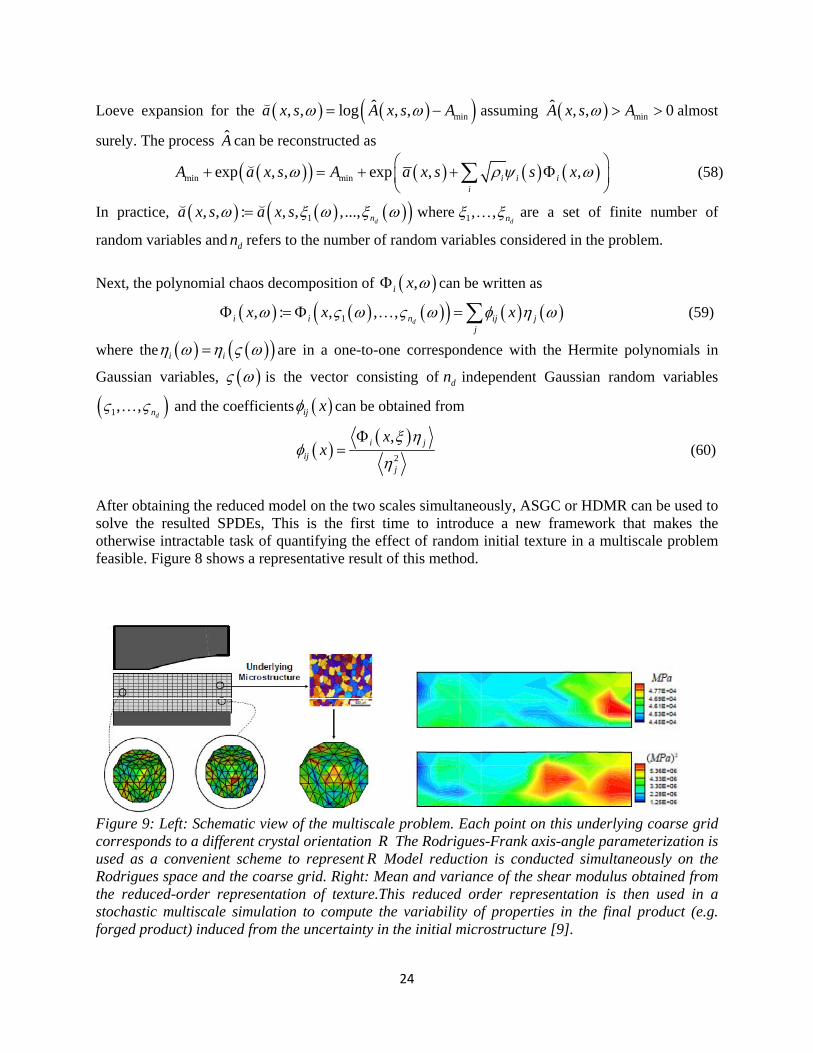
After obtaining the reduced model on the two scales simultaneously, ASGC or HDMR can be used to solve the resulted SPDEs, This is the first time to introduce a new framework that makes the otherwise intractable task of quantifying the effect of random initial texture in a multiscale problem feasible. Figure 8 shows a representative result of this method.

Figure 9: Left: Schematic view of the multiscale problem. Each point on this underlying coarse grid corresponds to a different crystal orientation R The Rodrigues-Frank axis-angle parameterization is used as a convenient scheme to represent R Model reduction is conducted simultaneously on the Rodrigues space and the coarse grid. Right: Mean and variance of the shear modulus obtained from the reduced-order representation of texture.This reduced order representation is then used in a stochastic multiscale simulation to compute the variability of properties in the final product (e.g. forged product) induced from the uncertainty in the initial microstructure [9].

25  

In closing, we note that in [13,14] and in an a number of additional forthcoming publications, we have extended all of the stochastic multiscale polycrystal material models discussed above to include in addition to texture uncertainty also grain size uncertainty. These models are based on enhanced physical modeling to account for the effect of grain size distribution on macroscale properties. The model reduction techniques (manifold learning) have been extended to work on high-dimensional microstructures defined in both the texture and grain size random space. This not only resulted in appropriate definition of distance metrics and properties of the microstructure manifold but also in a number of necessary extensions of the MaxEnt techniques needed to compute the probabilistic distribution of the underlying random variables. At the end of this work, we have managed to produce the convex hull of all material properties that should be expected (with the corresponding probabilities) in the presence of microstructure uncertainty. This has implications in the design of new materials, on prediction of rare events (e.g. failure due to extremal properties), etc. Acknowledgment/Disclaimer This work was sponsored by the Air Force Office of Scientific Research, USAF, under grant/contract number FA9550-07-1-0139. The views and conclusions contained herein are those of the authors and should not be interpreted as necessarily representing the official policies or endorsements, either expressed or implied, of the Air Force Office of Scientific Research or the U.S. Government. References [1] B. Ganapathysubramanian and N. Zabaras, "Modeling diffusion in random heterogeneous media: Data-driven models, stochastic collocation and the variational multiscale method", Journal of Computational Physics, Vol. 226, pp. 326-353, 2007. [2] B. Ganapathysubramanian and N. Zabaras, "A non-linear dimension reduction methodology for generating data-driven stochastic input models", Journal of Computational Physics, Vol. 227, pp. 6612-6637, 2008. [3] B. Ganapathysubramanian and N. Zabaras, "A seamless approach towards stochastic modeling: Sparse grid collocation and data driven input models", Finite Elements in Analysis and Design, Vol. 44, Issue 5, pp. 298-320, 2008. [4] B. Ganapathysubramanian and N. Zabaras, "Sparse grid collocation methods for the stochastic natural convection problems", Journal of Computational Physics, Vol. 225, pp. 652-685, 2007. [5] X. Ma and N. Zabaras, "An adaptive hierarchical sparse grid collocation algorithm for the solution of stochastic differential equations", Journal of Computational Physics, Vol. 228, pp. 3084-3113, 2009. [6] X. Ma and N. Zabaras, An efficient high-dimensional stochastic model representation technique for the solution of stochastic PDEs, J. Comput. Physics, in press. [7] B. Ganapathysubramanian and N. Zabaras, "A stochastic multiscale framework for modeling flow through heterogeneous porous media", Journal of Computational Physics, Vol. 228, pp. 591-618, 2009. [8] B. Kouchmeshky and N. Zabaras, “The effect of multiple sources of uncertainty on the convex hull of material properties of polycrystals”, Computational Materials Science, Vol. 47, pp 342-352, 2009. [9] B. Kouchmeshky and N. Zabaras, “Microstructure model reduction and uncertainty quantification in multiscale deformation processes”, Submitted.

26  

[10] N. Zabaras and B. Ganapathysubramanian, "A scalable framework for the solution of stochastic inverse problems using a sparse grid collocation approach", Journal of Computational Physics, Vol. 227, pp. 4697-4735, 2008. [11] V. Sundararaghavan and N. Zabaras, “A multilength scale continuum sensitivity analysis for the control of texture-dependent properties in deformation processing”, International Journal of Plasticity, Vol. 24, pp. 1581-1605, 2008. [12] X. Ma and N. Zabaras, “An efficient Bayesian inference approach to inverse problems based on adaptive sparse grid collocation method”, Inverse Problems (Institute of Physics), Vol. 25, 035013 (27pp), 2009. [13] B. Win, Z. Li and N. Zabaras, “Heat conduction variability of anisotropic polycrystalline microstructures through dimensionality reduction techniques”, submitted. [14] Z. Li, B. Win and N. Zabaras, “Investigating mechanical response variability of polycrystalline microstructures through dimensionality reduction techniques”, submitted. Personnel Supported During Duration of Grant N. Zabaras (PI), X. Ma (PhD expected 2010), B. Ganapathysubramanian (now Assistant Professor, ISU, Ames, Iowa, PhD awarded 2008), B. Kouchmeshky (PhD awarded 2009) Affiliation: Cornell University. Publications As listed in the references. Additional publications and presentations can be found on our laboratory’s web site (http://mpdc.mae.cornell.edu/). AFRL Point of Contact This work is being communicated with the group of Dr. J. Simmons, AFRL/MLLM. New Discoveries and Software (a) Develop an HDMR framework to address the high-dimensionality of stochastic PDE systems, (b) Non-linear reduced order model that could capture correlations in non-linear spaces and efficiently represent/process information of complex structures, (c) developed a hierarchical adaptive sparse-grid collocation scheme that captures the crucial stochastic dimensions and thus solve problems which were earlier infeasible, (d) developed a variational stochastic multiscale framework for material systems, (e) developed a non-intrusive (collocation) framework for design of complex systems under uncertainty and applied it to the design of deformation processes of polycrystalline materials, (f) used the adaptive sparse grid collocation solver as a surrogate model for accelerating multiscale Bayesian inference approaches and finally (g) developed a maximum entropy based framework for predicting the effects of uncertainty in initial texture on macroscopic property variability in deformation processes of polycrystalline materials.

Several of the computational tools developed have become available to collaborators at other universities as well as to government laboratories.