development of a novel tilt-controlled narrow commuter vehicle
TRANSCRIPT

Development of a Novel Tilt-Controlled Narrow
Commuter Vehicle
Final Report
Prepared by: J. Gohl, R. Rajamani, P. Starr, L. Alexander
Department of Mechanical Engineering
University of Minnesota
CTS 06-05
HUMAN CENTERED TECHNOLOGY TO ENHANCE SAFETY AND TECHNOLOGY

Technical Report Documentation Page 1. Report No. 2. 3. Recipients Accession No.
CTS 06-05 4. Title and Subtitle 5. Report Date
May 2006 6.
Development of a Novel-Tilt Controlled Narrow Commuter Vehicle
7. Author(s) 8. Performing Organization Report No.
J. Gohl, R. Rajamani, P. Starr, L. Alexander 9. Performing Organization Name and Address 10. Project/Task/Work Unit No.
CTS Project Number 2001030 11. Contract (C) or Grant (G) No.
Department of Mechanical Engineering University of Minnesota 111 Church St SE Minneapolis, MN 55455 12. Sponsoring Organization Name and Address 13. Type of Report and Period Covered
Final Report 14. Sponsoring Agency Code
Intelligent Transportation Systems Institute Center for Transportation Studies University of Minnesota 511 Washington Avenue SE, Suite 200 Minneapolis, MN 55455
15. Supplementary Notes
http://www.cts.umn.edu/pdf/CTS-06-05.pdf 16. Abstract (Limit: 200 words)
Traffic congestion is growing in urban areas of every size and is expected to double by 2010. A relatively unexplored but very promising solution to the problem of congestion is the adoption of narrow vehicles for commuter travel. Narrow vehicles like motorcycles can promote significantly improved highway utilization by the use of half-width lanes. However, in order for the general public to adopt this form of personal transportation, narrow vehicles should perceptibly provide the same ease of use and the same level of safety as passenger sedans. The research team in this project has developed a new concept vehicle that is relatively tall compared to its track width so as to provide a travel height that is comparable to that of other vehicles on the highway. To help the driver balance a relatively tall, narrow vehicle, it incorporates an electronic tilt control system that ensures tilt stability. The tilt control system balances the vehicle and improves ease of use, especially on curves where the vehicle must lean into the curve to ensure tilt stability. In this report the design and implementation of a control system that ensures the tilt stability of the prototype narrow vehicle is presented. The control system is based on the use of steer-by-wire technology and is called Steering Tilt Control (STC). The report includes significant details on the design of the prototype narrow vehicle constructed by the research team, on dynamic modeling for narrow tilting vehicles and also includes experimental results on the performance of the control system on the prototype narrow vehicle. 17. Document Analysis/Descriptors 18.Availability Statement
Narrow commuter vehicle, narrow tilting vehicle, tilt control, rollover control, rollover prevention, covered motorcycle
No restrictions. Document available from: National Technical Information Services, Springfield, Virginia 22161
19. Security Class (this report) 20. Security Class (this page) 21. No. of Pages 22. Price
Classified Classified 189

Development of a Novel Tilt-Controlled Narrow Commuter Vehicle
Final Report
Prepared by: J. Gohl
R. Rajamani P. Starr
L. Alexander
Department of Mechanical Engineering University of Minnesota
May 2006
Intelligent Transportation Systems Institute Center for Transportation Studies
University of Minnesota
CTS 06-05

Development of a Novel Tilt-Controlled
Narrow Commuter Vehicle
Final Report
J. Gohl, R. Rajamani, P. Starr and L. Alexander
Department of Mechanical Engineering
University of Minnesota

Executive Summary
Traffic congestion is growing in urban areas of every size and is expected to double by 2010. A
relatively unexplored but very promising solution to the problem of congestion is the adoption of narrow
vehicles for commuter travel. Narrow vehicles like motorcycles can promote significantly improved
highway utilization by the use of half-width lanes. However, in order for the general public to adopt this
form of personal transportation, narrow vehicles should perceptibly provide the same ease of use and the
same level of safety as passenger sedans.
The research team in this project has developed a new concept vehicle that is relatively tall
compared to its track width so as to provide a travel height that is comparable to that of other vehicles on
the highway. To help the driver balance a relatively tall, narrow vehicle, it incorporates an electronic tilt
control system that ensures tilt stability. The tilt control system balances the vehicle and improves ease
of use, especially on curves where the vehicle must lean into the curve to ensure tilt stability.
In this report the design and implementation of a control system that ensures the tilt stability of
the prototype narrow vehicle is presented. The control system is based on the use of steer-by-wire
technology and is called Steering Tilt Control (STC). The STC system uses steer-by-wire operation in
which the front wheel steering angle is used to control tilt while at the same time perceptibly allowing
the driver to use the steering angle for purposes of lateral control. A novel innovative algorithm is
presented for STC that satisfies both the driver handling requirements and the tilt stability re-
quirements.
The report includes significant detail on the design of the prototype narrow vehicle constructed
by the research team. Significant details on dynamic modeling for narrow tilting vehicles are presented.
The report also includes experimental results on the performance of the control system on the
prototype narrow vehicle. Comparisons are made between the simulated system and the experimental
vehicle. This illustrates the limitations encountered in the simulations but also shows
i

similarities that validate the model. Also, experimental results show that the vehicle is stabilized very
well by the controller within the limitations of our prototype hardware.
Future work on the narrow vehicle should include the development of a direct tilt control system in
the vehicle suspension so as to enable good control at low vehicle speeds.
ii

Table of Contents
Page
Executive Summary........................................................................................................................... i
List of Figures ................................................................................................................................ vi
List of Tables ..................................................................................................................................... x
ChapterI. Introduction ................................................................................................................... 1
ChapterII. Dynamic Model .............................................................................................................. 8
2.1 Nonlinear Model.................................................................................................. 8
2.2 Equilibrium Solution .......................................................................................... 9
2.3 Linearized Model................................................................................................. 17
Chapter III. Control Schemes .............................................................................................................. 23
3.1 Lateral Based Control......................................................................................... 25
3.1.1 Steering Assist, Independent Driver and Tilting Controller . . 27
3.1.2 Steer-by-Wire, Lateral State Observer (LSO)...................................... 29
3.2 Steer-by-Wire, Desired Lean Angle (DLA) ..................................................... 35
Chapter IV. Simulations................................................................................................................ ......... 42
4.1 Matlab/Simulink................................................................................................. 42
4.1.1 Lateral Implications ............................................................................. 42
4.1.2 Lateral State Observer......................................................................... 47
4.1.3 Desired Lean Angle, Steer-by-Wire...................................................... 51
4.2 Visual Basic .................................................................................................... 56
4.2.1 Program Description............................................................................ 56
4.2.2 Results ............................................................................................. 58
iii

Page
Chapter V. Experimental Vehicle . . . . .
. . . . . . . . . . . . . . . . . . . . . . . . . . . . 62
5.1 Vehicle Description . . . . . . . . . . . . . . . . . . . . . . . . . . . . . 62
5.1.1 Drive Unit . . . . . . . . . . . . . . . . . . . . . . . . . . . . . 64
5.1.2 Chassis . . . . . . . . . . . . . . . . . . . . . . . . . . . . . . . 64
5.1.3 Outriggers . . . . . . . . . . . . . . . . . . . . . . . . . . . . . . 66
5.1.4 Electrical Power . . . . . . . . . . . . . . . . . . . . . . . . . . 66
5.1.5 Computer . . . . . . . . . . . . . . . . . . . . . . . . . . . . . . 66
5.1.6 Steering . . . . . . . . . . . . . . . . . . . . . . . . . . . . . . . 67
5.1.7 RC User Inputs . . . . . . . . . . . . . . . . . . . . . . . . . . . 70
5.1.8 Sensors . . . . . . . . . . . . . . . . . . . . . . . . . . . . . . . 72
5.1.9 Antialiasing Filters . . . . . . . . . . . . . . . . . . . . . . . . . 75
5.2 Parameter Estimation . . . . . . . . . . . . . . . . . . . . . . . . . . . . 75
Chapter VI. Experimental Results . . . . .
. . . . . . . . . . . . . . . . . . . . . . . . . . . . 84
6.1 Model Validation . . . . . . . . . . . . . . . . . . . . . . . . . . . . . . . 86
6.2 Vehicle Open Loop Response . . . . . . . . . . . . . . . . . . . . . . . . 95
6.3 Vehicle Closed Loop Response . . . . . . . . . . . . . . . . . . . . . . . 99
6.4 Unstable Oscillations . . . . . . . . . . . . . . . . . . . . . . . . . . . . 109
6.5 Unmodeled Dynamics . . . . . . . . . . . . . . . . . . . . . . . . . . . . 117
Chapter VII. Summary and Conclusions . . . . . . . . . . . . . . . . . . . . . . . . . . . . . 122
Appendix A. Coordinate Systems . . . . . . . . . . . . . . . . . . . . . . . . . . . . . 126
Appendix B. Symbols and Notation . . . . . . . . . . . . . . . . . . . . . . . . . . . . 131
B.1 Notation . . . . . . . . . . . . . . . . . . . . . . . . . . . . . . . . . . . 131
B.2 Vehicle Speci…c Symbols . . . . . . . . . . . . . . . . . . . . . . . . . . . 131
B.2.1 Constant Terms . . . . . . . . . . . . . . . . . . . . . . . . . . 131
B.2.2 State and State Dependent Terms . . . . . . . . . . . . . . . . 133
iv

Page
Appendix C. Dynamic Model Derivation . . . . . . . . . . . . . . . . . . . . . . . . . 135
C.1 Vehicle Body . . . . . . . . . . . . . . . . . . . . . . . . . . . . . . . . . 135
C.1.1 Translational Balance . . . . . . . . . . . . . . . . . . . . . . . 135
C.1.2 Moment Balance . . . . . . . . . . . . . . . . . . . . . . . . . . 142
C.2 Front Wheels . . . . . . . . . . . . . . . . . . . . . . . . . . . . . . . . . 144
C.2.1 Translational Balance . . . . . . . . . . . . . . . . . . . . . . . 144
C.2.2 Moment Balance . . . . . . . . . . . . . . . . . . . . . . . . . . 148
C.3 Rear Wheel . . . . . . . . . . . . . . . . . . . . . . . . . . . . . . . . . . 156
C.3.1 Translational Balance . . . . . . . . . . . . . . . . . . . . . . . 156
C.3.2 Moment Balance . . . . . . . . . . . . . . . . . . . . . . . . . . 158
C.4 Total Model . . . . . . . . . . . . . . . . . . . . . . . . . . . . . . . . . 160
C.4.1 Translational Balance . . . . . . . . . . . . . . . . . . . . . . . 160
C.4.2 Moment Balance . . . . . . . . . . . . . . . . . . . . . . . . . . 160
C.4.3 Nonlinear Closed Form . . . . . . . . . . . . . . . . . . . . . . 164
C.5 Model Linearization . . . . . . . . . . . . . . . . . . . . . . . . . . . . . 166
C.6 Error Coordinates . . . . . . . . . . . . . . . . . . . . . . . . . . . . . . 171
References . . . . . . . . . . . . . . . . . . . . . . . . . . . . . . . . . . . . . . . . . . . 175
v

List of Figures
1.1 Tipping Statics Diagram . . . . . . . . . . . . . . . . . . . . . . . . . . . . . . 2
1.2 F 300 Life-Jet front cornering view . . . . . . . . . . . . . . . . . . . . . . . . 4
1.3 F 300 Life-Jet side view . . . . . . . . . . . . . . . . . . . . . . . . . . . . . . . 4
1.4 The GM Lean Machine . . . . . . . . . . . . . . . . . . . . . . . . . . . . . . . 5
2.1 Steady state yaw rate for vehicle based on equation 18 . . . . . . . . . . . . . 12
2.2 Two wheeled ground plane projection . . . . . . . . . . . . . . . . . . . . . . . 13
2.3 Steady state manuever curvature based on equation 38 . . . . . . . . . . . . . 15
2.4 Curvature estimation error by using equation 41 . . . . . . . . . . . . . . . . . 16
3.1 Block diagram of a motorcyle/driver system, (18:pp. 14) . . . . . . . . . . . . 23
3.2 DTC block diagram . . . . . . . . . . . . . . . . . . . . . . . . . . . . . . . . . 24
3.3 STC block diagram . . . . . . . . . . . . . . . . . . . . . . . . . . . . . . . . . 24
3.4 Unstable tilt control con…guration . . . . . . . . . . . . . . . . . . . . . . . . . 27
3.5 Inner loop block diagram . . . . . . . . . . . . . . . . . . . . . . . . . . . . . . 37
3.6 Nyquist plot of G(s)H(s). . . . . . . . . . . . . . . . . . . . . . . . . . . . . . 39
3.7 Closed loop bode diagram without derivative control term . . . . . . . . . . . 40
3.8 Closed loop bode diagram with derivative control term . . . . . . . . . . . . . 41
4.1 Window de…nitions for approximating step curvature input . . . . . . . . . . . 45
4.2 Desired global trajectory for 3 window lengths, R = 7.0m . . . . . . . . . . . . 46
4.3 Desired global trajectory with shifted window, R = 7.0 m . . . . . . . . . . . . 47
4.4 LSO controlled vehicle global trajectory . . . . . . . . . . . . . . . . . . . . . . 48
4.5 LSO controlled vehicle lean angle . . . . . . . . . . . . . . . . . . . . . . . . . 49
4.6 LSO controlled vehicle steering outputs . . . . . . . . . . . . . . . . . . . . . . 50
4.7 LSO controlled vehicle plant input . . . . . . . . . . . . . . . . . . . . . . . . . 51
4.8 DLA controlled vehicle with derivative term, lean angle step response . . . . . 52
4.9 DLA controlled vehicle without derivative term, lean angle step response . . . 53
vi

Figure Page
4.10 DLA controlled vehicle global trajectory . . . . . . . . . . . . . . . . . . . . . 54
4.11 DLA controlled vehicle lean angle . . . . . . . . . . . . . . . . . . . . . . . . . 55
4.12 DLA controlled vehicle plant input . . . . . . . . . . . . . . . . . . . . . . . . 56
4.13 User interface for real time simulator . . . . . . . . . . . . . . . . . . . . . . . 57
4.14 Real time simulator, vehicle global trajectory, 0 - 80s . . . . . . . . . . . . . . 58
4.15 Real time simulator, vehicle global trajectory, 0 - 20s . . . . . . . . . . . . . . 59
4.16 Real time simulator, vehicle lean angle, 0 - 80s . . . . . . . . . . . . . . . . . . 60
4.17 Real time simulator, vehicle lean angle power spectrum . . . . . . . . . . . . . 61
5.1 Vehicle in parking lot . . . . . . . . . . . . . . . . . . . . . . . . . . . . . . . . 62
5.2 Vehicle front view . . . . . . . . . . . . . . . . . . . . . . . . . . . . . . . . . . 63
5.3 Front chassis view . . . . . . . . . . . . . . . . . . . . . . . . . . . . . . . . . . 63
5.4 Schematic view of front chassis . . . . . . . . . . . . . . . . . . . . . . . . . . . 64
5.5 Vehicle Tilting Components . . . . . . . . . . . . . . . . . . . . . . . . . . . . 65
5.6 Steering error PSD for high and low sprocket ratios . . . . . . . . . . . . . . . 69
5.7 User input signal PSD, …ltered and un…ltered . . . . . . . . . . . . . . . . . . 71
5.8 Tilt and tilt rate measurement . . . . . . . . . . . . . . . . . . . . . . . . . . . 74
5.9 Center of gravity height estimation schematic . . . . . . . . . . . . . . . . . . 76
5.10 Center of gravity height estimation data . . . . . . . . . . . . . . . . . . . . . 78
5.11 Predicted tipping response of vehicle for various values of Ixx . . . . . . . . . 79
5.12 Lateral motion parameter estimation block diagram . . . . . . . . . . . . . . . 81
5.13 Simulated vehicle tilt for lateral mode parameter estimation . . . . . . . . . . 82
5.14 Simulated vehicle yaw rate for lateral mode parameter estimation . . . . . . . 82
6.1 Control loop realization . . . . . . . . . . . . . . . . . . . . . . . . . . . . . . . 84
6.2 Actual vehicle tilting response . . . . . . . . . . . . . . . . . . . . . . . . . . . 86
6.3 Actual vehicle speed response . . . . . . . . . . . . . . . . . . . . . . . . . . . 87
6.4 Actual vehicle yaw rate . . . . . . . . . . . . . . . . . . . . . . . . . . . . . . . 88
6.5 Estimated transfer function magnitude: desired steer angle to vehicle tilt . . . 89
vii

Figure Page
6.6 Estimated transfer function phase: desired steer angle to vehicle tilt . . . . . . 90
6.7 Estimated transfer function magnitude: desired steering to yaw rate . . . . . . 91
6.8 Estimated transfer function phase: desired steering to yaw rate . . . . . . . . 91
6.9 Estimated transfer function magnitude: driver output to vehicle tilt . . . . . . 92
6.10 Estimated transfer function phase: driver output to vehicle tilt . . . . . . . . . 93
6.11 Estimated transfer function magnitude: driver output to yaw rate . . . . . . . 94
6.12 Estimated transfer function phase: driver output to yaw rate . . . . . . . . . . 94
6.13 Open loop tilting response . . . . . . . . . . . . . . . . . . . . . . . . . . . . . 96
6.14 Open loop speed response . . . . . . . . . . . . . . . . . . . . . . . . . . . . . 97
6.15 Open loop yaw rate response . . . . . . . . . . . . . . . . . . . . . . . . . . . . 98
6.16 Closed loop tilting response . . . . . . . . . . . . . . . . . . . . . . . . . . . . 99
6.17 Continuous time control loop representation . . . . . . . . . . . . . . . . . . . 100
6.18 Continuous time control loop simpli…cation . . . . . . . . . . . . . . . . . . . . 101
6.19 Relative tilt error magnitude for approximate step input . . . . . . . . . . . . 102
6.20 Closed loop yaw rate response . . . . . . . . . . . . . . . . . . . . . . . . . . . 103
6.21 Closed loop speed response . . . . . . . . . . . . . . . . . . . . . . . . . . . . . 104
6.22 Closed loop steering error data . . . . . . . . . . . . . . . . . . . . . . . . . . . 105
6.23 November 23, 2002 run 2 data . . . . . . . . . . . . . . . . . . . . . . . . . . . 106
6.24 November 23, 2002 run 4 data . . . . . . . . . . . . . . . . . . . . . . . . . . . 106
6.25 November 23, 2002 run 5 data . . . . . . . . . . . . . . . . . . . . . . . . . . . 107
6.26 November 23, 2002 run 16 data . . . . . . . . . . . . . . . . . . . . . . . . . . 107
6.27 November 28, 2002 run 5 data . . . . . . . . . . . . . . . . . . . . . . . . . . . 108
6.28 November 28, 2002 run 14 data . . . . . . . . . . . . . . . . . . . . . . . . . . 108
6.29 Vehicle tilting data, apparent instability . . . . . . . . . . . . . . . . . . . . . 109
6.30 Vehicle tilt angle PSD of unstable region . . . . . . . . . . . . . . . . . . . . . 110
6.31 Vehicle steering error data . . . . . . . . . . . . . . . . . . . . . . . . . . . . . 111
6.32 Steering angle command . . . . . . . . . . . . . . . . . . . . . . . . . . . . . . 112
viii

Figure Page
6.33 Steering error and tilt angle PSD’s . . . . . . . . . . . . . . . . . . . . . . . . 113
6.34 Control loop simpli…cation 1 . . . . . . . . . . . . . . . . . . . . . . . . . . . . 114
6.35 Control loop simpli…cation 2 . . . . . . . . . . . . . . . . . . . . . . . . . . . . 114
6.36 Open loop magnitude data, ue . . . . . . . . . . . . . . . . . . . . . . . . . . . 116
6.37 Open loop phase data, ue . . . . . . . . . . . . . . . . . . . . . . . . . . . . . . 117
6.38 Wobble mode perturbation, Tilt angle response . . . . . . . . . . . . . . . . . 118
6.39 Wobble mode perturbation, tilt angle and yaw rate PSD . . . . . . . . . . . . 119
6.40 Wobble mode in‡uence on tilt angle data . . . . . . . . . . . . . . . . . . . . . 120
6.41 Wobble mode in‡uence on yaw rate data . . . . . . . . . . . . . . . . . . . . . 120
6.42 Open loop yaw rate PSD . . . . . . . . . . . . . . . . . . . . . . . . . . . . . . 121
A.1 Coordinates sytems 1 and 4 . . . . . . . . . . . . . . . . . . . . . . . . . . . . 126
A.2 Vehicle body, body …xed coordinate systems 3 and 4 . . . . . . . . . . . . . . 127
A.3 Vehicle body, body …xed coordinate system 5 with respect to system 3 . . . . 128
A.4 Front wheel, body …xed coordinate system 6 with respect to system 5 . . . . . 128
C.1 Front wheel side view: trail schematic . . . . . . . . . . . . . . . . . . . . . . . 155
C.2 Top view schematic of vehicle with relavent slip angle velocities . . . . . . . . 168
ix

List of Tables
2.1 Plant eigenvalues . . . . . . . . . . . . . . . . . . . . . . . . . . . . . . . . . . 22
3.1 Control loop eigenvalues . . . . . . . . . . . . . . . . . . . . . . . . . . . . . . 29
3.2 Closed loop eigenvalues . . . . . . . . . . . . . . . . . . . . . . . . . . . . . . . 29
3.3 Total closed loop eigenvalues . . . . . . . . . . . . . . . . . . . . . . . . . . . . 34
3.4 Leaning vehicle closed inner loop eigenvalues with PD controller . . . . . . . . 41
5.1 Center of gravity height estimation data . . . . . . . . . . . . . . . . . . . . . 77
5.2 Lateral mode parameter values . . . . . . . . . . . . . . . . . . . . . . . . . . . 81
x

Narrow Tilting Vehicle: Modeling and Control
Chapter I. Introduction
With increased tra¢c congestion on today’s roads comes increased interest in new solutions.
Many solutions rely on increasing person per vehicle statistics by the use of mass transit or
carpooling. This is done, in the case of mass transit, by using larger vehicles to accommodate more
riders per vehicle. In the case of carpooling, the existing vehicles’ person per vehicle number is
increased to be closer to its capacity. The goal of this is to increase the ‡ow rate of a particular
tra¢c artery. A converse approach to increase the ‡ow rate would be not to make the vehicles
larger but to make the vehicles smaller. In this way, although the person per vehicle number might
only be one but the capacity of the smaller vehicle might only be one or two. In this way, the
average person per vehicle number would be over 50% of a vehicle’s capacity. The bene…t to overall
tra¢c ‡ow then, comes from …tting more vehicles on a lane and so increasing the ‡ow rate.
It’s true that there will be many issues to address before wide scale implementation of such a
system could be started. Questions like, what will be the expected increase in ‡ow rate? How will
the smaller vehicles interact or even con‡ict with larger vehicles also using the roads? Along with
these questions are human factors issues. Will there be signi…cant changes to driving habits? What
will be the perception of smaller vehicles? Certainly there are questions of safety. For instance,
what happens in a crash? Also, there are technical questions to ask. How fast can a smaller vehicle
accelerate and travel? What is the most e¢cient propulsion? Finally, there is a question of stabil-
ity. Will the vehicle tip over and what can be done to prevent it? This is the problem of concern in
this paper.
Narrow vehicles that do not lean are unstable when they corner too hard. A simple statics
calculation can illustrate this fact. Imagine looking at the front of a vehicle as it accelerates toward
1

the right as in Figure 1.1. This …gure shows the equipollent moment and force action on the
center of gravity of the vehicle leaning at an angle θ.
Rl
F/2 F/2Rr
2b
mg
θ
h =
TF=hF·cosθ =hma·cosθ
a
TR=(b+h·sinθ)Rl=(b+h·sinθ)mg
Figure 1.1 Tipping Statics Diagram
Label the height of the center of gravity as h, and the wheelbase width as 2b. Then as
the vehicle accelerates to the right in a turn, due to increasing F , Rr approaches zero while Rl
approaches mg. At this limit F = ma so that TF = hF cos θ = hma cos θ and TR = (b + h sin θ)mg.
TR refers to the moment due to the normal reactions and TF refers to the moment due to the lateral
forces. Stability is maintained if TF < TR this implies stability for a < g b+h sin θh cos θ . By introducing
tilt we increase the limit on a. In the next section we will use the nonlinear model to derive a
relation between the lateral acceleration, a , the vehicle’s yaw rate and velocity at steady state. As
expected, this will also be related to the lean and steady state steer angle.
From this discussion, a solution to the tipping problem for a narrow vehicle, it seems, is to lean
while cornering. It turns out that motorcycles have already addressed this issue. Since they are
the limiting case for narrow vehicles, they must lean while cornering. One of the di¢culties of wide
spread implementation for relieving tra¢c in this way is that it takes practice to ride a motorcycle
well, see (29:pp. 68) and (22). In the absence of experience, they can be dangerous. The following
2

statement was taken from a brochure issued by the National Highway Tra¢c Safety Administration
(42):
"...The causes of many motorcycle crashes can be attributed to:
² lack of basic riding skills
² failure to appreciate the inherent operating characteristics
² failure to appreciate the limitations of the motorcycle
² failure to use special precautions while riding
² failure to use defensive driving techniques
² lack of speci…c braking and cornering skills
² failure to follow speed limit"
Now this is not a paper on the dangers of motorcycles but these issues do illustrate the point
that experience and skill is necessary to drive one safely. Also, if wide scale implementation is to
occur for narrow/leaning commuter vehicles, they had better be easy to drive.
There is a fundamental di¤erence between driving a non-leaning vehicle versus a free leaning
vehicle. The second issue stated above regarding the "inherent operating characteristics", is primar-
ily due to counter-steer. A motorcycle requires counter steer to change directions. To maneuver a
non-leaning vehicle, however, simply requires the steering wheel be turned in the desired direction
of travel. This creates problems when switching from one type of vehicle to another, especially
when a fast maneuver is necessary in an emergency situation. The project objective was to design
a controller that would make driving a narrow tilting vehicle as easy for anyone to do without any
motorcycle riding experience. We explored possible controllers and analyzed their usefulness both in
stabilizing the vehicle and in interacting with the driver.
3

Other groups have also studied vehicles of this type. The "F 300 Life-Jet" shown in Figures
1.2 and 1.3 is a three wheeled tilting concept vehicle built by Mercedes-Benz. General Motors was
also involved in some research with leaning vehicles. The "Lean Machine" shown in Fgure 1.4 is a
concept vehicle built by GM. These photos were obtained from the websites listed in references
(43) and
(44), respectively.
Figure 1.2 F 300 Life-Jet front cornering view
Figure 1.3 F 300 Life-Jet side view
4

Figure 1.4 The GM Lean Machine
The design of leaning vehicles is a challenge that goes beyond a simple research project.
Even respected car companies see the possible bene…ts of this type of vehicle.
A narrow tilting vehicle (NTV) has some similarities to the classic control problem of the
inverted pendulum. In the classic inverted pendulum problem, the system dynamics have two real
valued poles with equal magnitude but opposite sign. One pole is stable while the other is unstable.
The magnitude of these poles is determined by the mass, height of the center of gravity, acceleration
of gravity and the moment of inertia. In the NTV, we still have approximately these poles along
with poles due to the lateral dynamics. The tilting poles are shifted slightly due to coupling between
the tilting and lateral modes. With the inverted pendulum, active control must be applied to
stabilize the tilting. This also occurs with an NTV. On a motorcycle, the rider performs this function
in conjunction with controlling the lateral motion. To control the tilting automatically on an NTV,
as we would like to do, there are two distinct methods. The two methods are Direct Tilt Control
(DTC) and Steering Tilt Control (STC), see (2).
Direct tilt control uses an actuator to apply a leaning torque directly to the leaning dynamics
of the vehicle. This allows the controller to position the vehicle at any desired angle. There are two
important issues to address with the DTC method. The …rst is determining the desired lean
angle
5

of the vehicle. In some way, the driver’s actions must determine the required lean angle for a desired
maneuver. Interpreting these intentions is not a trivial task and requires thoughtful consideration.
The second issue is reducing the torque that an actuator needs to exert. Even though a vehicle in
a perfectly coordinated turn is at an equilibrium position (and hence only requires small torque for
small deviations), getting to that point can require large peaks in the applied torque.
The other method, the one studied in this paper, is STC. The control input that balances
the vehicle is the lateral force between the road and the wheels. This is the same lateral force that
controls the lateral modes of the vehicle. In our case we modeled this force with slip angles of the
wheels such that the control input to the system plant is the front wheel angle. Because the input
depends on the steering, this method is called “Steering Tilt Control”, (2). Since the control input
in‡uences both modes, we need to account for this when designing the tilt controller. We need
to be aware that one mode can destabilize the other. This type of control is the same method
used by bicycle and motorcycle riders to balance the vehicle. This active control is most apparent
at slow speeds and becomes less so at higher speeds when the gyroscopic moments are greater.
This is especially true on motorcycles where the wheels can have signi…cant mass. An interesting
phenomenon already hinted at that arises in this system is counter-steering. Experienced motorcycle
riders are often familiar with this such that a negative steering input must be given to attain the
proper lean angle prior to entering a steady state turn. This behavior can be demonstrated from
the dynamic model and is part of the reason that it takes practice to pro…ciently ride a motorcycle.
This is fundamentally di¤erent from driving a non-leaning automobile.
Many of the research projects we found relating to tilting vehicles used either DTC or driver
controlled STC. The F 300 Life-Jet for instance seems to use DTC with an hydraulic actuator.
Most of the details of the F 300 Life-Jet, however, are proprietary. Other leaning vehicle projects
include, but are not limited to, the GM Lean Machine, which uses a driver controlled DTC, and the
Millennium Tracer, (45), which uses driver controlled STC. The website listed in reference (44) is a
6

good source for further information on the subject. The lack of experimental results on automatic
STC is the void this research aims to …ll.
Ultimately, a combination of both DTC and STC would be needed for a useful vehicle. DTC
is needed to keep the vehicle upright at slow speeds and when the vehicle is stopped. This will be
shown from the vehicle model in the next section. STC, conversely, is a good control method at
higher speeds. This paper represents a starting point to implementing STC on a vehicle.
7

Chapter II. Dynamic Model
We started the process of designing a controller by deriving a model for the system. The derivation
of this model is described in appendix C. Some of the highlights of this are shown here.
2.1 Nonlinear Model
The nonlinear equations are derived as equations 311, 315, and 316. By neglecting the terms
Dx5 , Dy
4 , and Dz5 we get the nonlinear dynamic model listed here as equations 1 to 3.
Ä ψ ((cos θ) Izz + (tan θ) (sin θ) Iyy)
= 2_θ _
ψ (sin θ) (Izz ¡ Iyy)
+ (2Ff lf ¡ Frlr) ((tan θ) (sin θ) + (cos θ)) (1)
Ä θ = 1
J
³mgh (sin θ) ¡ h2m (cos θ sin θ) _ θ
2
+ 1
J
³ _ ψ2 (cos θ sin θ) (Iyy ¡ Izz) ¡ h (2Ff + Fr) (cos θ)
´(2)
Ä y = ¡v _ψ ¡ 1
J gh2m cos θ sin θ + h _θ
2µ
(sin θ) + 1
J h2m cos2 θ sin θ
¶
+h _ψ2µ
sin θ + 1
J
¡cos2 θ sin θ
¢ (Izz ¡ Iyy)
¶
+ (2Ff + Fr)
µ 1
J h2 cos2 θ +
1
m
¶(3)
The …rst step in analyzing any nonlinear dynamic equations is usually to search for any equilibrium
solutions. To start this process, let us make the following variable substitutions:
x =
·x1 x2 x3 x4 x5 x6
¸T
(4)
x1 = y, x2 = _ y, x3 = ψ, x4 = _ψ, x5 = θ, x6 = _θ (5)
8

Using these de…nitions with equations 1 - 3, we get the …rst order model equations 6 - 12.
_x1 = f1(x) = x2 (6)
_x2 = f2(x) = ¡v _ψ ¡ 1
Jgh2m cos θ sin θ
+h _θ2µ
(sin θ) +1
Jh2m cos2 θ sin θ
¶
+h _ψ2µ
sin θ +1
J
¡cos2 θ sin θ
¢ ³Iz2 ¡ Iy2
´¶
+(2Ff + Fr)
µ1
Jh2 cos2 θ +
1
m
¶(7)
_x3 = f3(x) = x4 (8)
_x4 = f4 (x) =
³2_θ _ψ (sin θ) (Izz ¡ Iyy) + (2Ff lf ¡ Frlr) ((tan θ) (sin θ) + (cos θ))
´/ (9)
((cos θ) Izz + (tan θ) (sin θ) Iyy) (10)
_x5 = f5(x) = x6 (11)
_x6 = f6 (x) =1
J
³mgh (sin θ) ¡ h2m (cos θ sin θ) _θ
2´
+1
J
³_ψ2(cos θ sin θ) (Iyy ¡ Izz) ¡ h (2Ff + Fr) (cos θ)
´(12)
2.2 Equilibrium Solution
Now, an equilibrium solution, xss, must satisfy _x = 0. The trivial solution is of course one
possibility but the more interesting one comes from neglecting equation 8. In this case we get, from
equations 6 and 11, x2 = _y = 0 and x6 = _θ = 0. To start, we solve the steady state solution of
9

equation 7 for 2Ff + Fr. Doing so, we get:
(2Ff + Fr)
=
µv _ψss +
1
Jgh2m cos θss sin θss
¶1¡
1J h2 cos2 θss + 1
m
¢ (13)
¡µ
h _ψ2
ss
µsin θss +
1
J
¡cos2 θss sin θss
¢ ³Iz2 ¡ Iy2
´¶¶1¡
1J h2 cos2 θss + 1
m
¢ (14)
This expression is then used in the steady state solution to equation 12, f6 (x) = 0. Upon simpli…-
cation, we get:
¡Iyy ¡ Izz + mh2
¢_ψ2
ss sin θss cos θss ¡ mhv (cos θss) _ψss + mgh sin θss = 0 (15)
This becomes:
1
mgh
¡Iyy ¡ Izz + mh2
¢(sin θss) _ψ
2
ss ¡ v
g_ψss + tan θss = 0 (16)
Which is a quadratic expression relating θss and v to _ψss. Assuming that Iyy ' Izz, the solutions
to this equation will have the form:
_ψss =1
2h sin θss
hv +
pv2 ¡ 4gh sin θss tan θss
i(17)
_ψss =1
2h sin θss
hv ¡
pv2 ¡ 4gh sin θss tan θss
i(18)
Observe that the limit of equation 17 as θss ! 0 does not exist. This is obvious by the computing
the limits of the numerator and denominator separately.
limθss!0
hv +
pv2 ¡ 4gh sin θss tan θss
i= 2v (19)
limθss!0
2h sin θss = 0 (20)
10

The limit of the other solution, equation 18, as θss ! 0 on the other hand is indeterminate but can
be shown to exist using L’Hopital’s rule (41:pp. 79).
limθss!0
hv ¡
p v2 ¡ 4gh sin θss tan θss
i= 0 (21)
limθss!0
2h sin θss = 0 (22)
Therefore, L’Hopital’s rule applies.
limθss!0
d
dθss
hv ¡
p v2 ¡ 4gh sin θss tan θss
i = 0 (23)
limθss!0
d
dθss (2h sin θss) = 2h (24)
Using this result:
limθss!0
_ ψss = 0 (25)
Now, for the solution given by equation 18 to be real we must have:
v2 ¡ 4gh sin θss tan θss ¸ 0 (26)
Or:
v ¸p
4 gh sin θss tan θss (27)
A typical value of θss might be 30± in which case with our value of h given in appendix B we get
the following limit on v:
v ¸ 1.68 m
s (28)
This is a lower limit on the velocity for an equilibrium solution to exist beyond 30± of lean. A plot
of equation 18 is shown in Figure 2.1.
11

Figure 2.1 Steady state yaw rate for vehicle based on equation 18
Now, the equilibrium solution to equation 9 is found:
f4 (x) = 0 =
(2Ff lf ¡ Frlr) ((tan θss) (sin θss) + (cos θss)) (29)
With the de…nitions of Ff and Fr given by equations 327 and 328, we get the following expression:
_ ψss ¡Ã
lrλr ¡ 2lf λf
Crl2r ¡ 2Cf l2fθss ¡ 2Cf
lf
Crl2r ¡ 2Cf l2fδss
! v = 0 (30)
Equation 30 along with equation 18 and x2 = _ y = 0 and x6 = _θ = 0 represents the steady
state solution with one degree of freedom. Throughout this project, we considered this solution
12

parameterized by θss. Thus, xss for the state space representation 339 becomes:
xss =
·0 _ ψss θss 0
¸T
(31)
Equation 30 will yield the standard kinematic steady state expressions δss = lR and _ψss = v
R under
certain vehicle con…gurations. First when there is no leaning, θss = 0, equation 30 becomes:
_ ψss = ¡2Cflf
Crl2r ¡ 2Cf l2fδssv (32)
Next, when there are an equal number of wheels on both the front and back all with the same slip
angle gains, Cf = Cr, equation 32 becomes:
_ ψss = ¡ lf
l2r ¡ l2fδssv = ¡ lf
(lr + lf ) (lr ¡ lf )δssv = ¡ lf
l ¢ (lr ¡ lf )δssv (33)
Now, let us look at a projection of a two wheeled vehicle con…guration in the ground plane.
lf
R'
R
R"
lr
l
δss
Front Wheel
Rear Wheel
Figure 2.2 Two wheeled ground plane projection
13

From this diagram, …gure 6, we get:
tan δss = l
R0 (34)
Which approximates to:
tan δss ' δss 'l
R0 (35)
when δss is small. Also, as lf ! l, R ! R0 and so we get:
δss = l
R (36)
Using this approximation equation 33 becomes:
_ ψss = ¡ lf
l ¢ (lr ¡ lf )δssv '
1
l δssv '
v
R = vCv (37)
This expression can be used to re-write equation 18 as:
Cv = 1
2vh sin θss
hv ¡
p v2 ¡ 4gh sin θss tan θss
i(38)
This substitution was made because the curvature is easier to interpret than the yaw rate since it
is simply the inverse of R which is an easy quantity to visualize. A plot of this solution for the
range of velocities and lean angles typical for a leaning vehicle is shown in Figure 2.3.
14

Figure 2.3 Steady state manuever curvature based on equation 38
Thus, the maneuver curvature is a way of parameterizing the equilibrium solution or desired
steady state motion of the vehicle. The last step of this section is to make an approximation to this
solution by assuming the second order term of equation 16 is negligible. This occurs when _ψss and
θss are small. Making this approximation, equation 16 becomes:
¡v
g _ψss + tan θss = 0 (39)
This simpli…es to the typical relation between θss and _ψss:
_ ψss = g
v tan θss (40)
Cv = g
v2 tan θss (41)
15

If equation 40 is linearized about θss = 0, we get:
_ ψss = g
v θss (42)
This shows the approximate linear nature between θss and _ψss via the coe¢cient g v . Also, as v
increases, the slope of this expression approaches zero. The di¤erence between equations 38 and 41
is a way of showing the error imposed by using equation 41 instead of equation 38. This is shown
in Figure 2.4.
Figure 2.4 Curvature estimation error by using equation 41
We see that except for large lean angles at slow speeds, this approximation results in reasonable
estimates of the maneuver curvature.
16

2.3 Linearized Model
The …nal linearized equations are found by evaluating the Jacobian of the system of equations
6 - 12 at the steady state solution. This linearized set of equations is parameterized by θss (and
_ψss which is itself parameterized by θss from equation 30).
_x = Ax + Bδ (43)
Where:
A =
·∂f
∂x
¸
x=xss
=
26666666666666666664
0 1 0 0 0 0
0 A2,2 0 A2,4 A2,5 A2,6
0 0 0 1 0 0
0 A4,2 0 A4,4 A4,5 A4,6
0 0 0 0 0 1
0 A6,2 0 A6,4 A6,5 A6,6
37777777777777777775
(44)
B =
·∂f
∂δ
¸
δ=δss
(45)
=
·0 B2 0 B4 0 B6
¸T
(46)
With the following expressions for the entries of the second row:
A2,2 =
·∂
∂ _yf2
¸
x=xss
= ¡1
v
µh2
Jcos2 θss +
1
m
¶(2Cf + Cr) (47)
A2,4 =
·∂
∂ _ψf2
¸
x=xss
= ¡v + 2
µIzz ¡ Iyy
Jcos2 θss + 1
¶h (sin θss) _ψss (48)
¡2Cf lf ¡ CrlrJv
h2 cos2 θss ¡ 2Cf lf ¡ Crlrvm
(49)
17

A2,5 =
·∂
∂θf2
¸
x=xss
=
µ¡2 (cos θss sin θss) θss + cos2 θss
Jh2 +
1
m
¶(2λf + λr) (50)
+h
µ3Izz ¡ 3Iyy
Jcos3 θss +
µ1 +
¡2Izz + 2Iyy
J
¶cos θss
¶_ψ2
ss (51)
+2h2 2Cf lf ¡ CrlrvJ
(cos θss) (sin θss) _ψss (52)
¡4h2 (cos θss sin θss)Cf
Jδ (53)
+1 ¡ 2 cos2 θss
Jmgh2 (54)
A2,6 =
·∂
∂ _θf2
¸
x=xss
= 0 (55)
For the forth row:
A4,2 =
·∂
∂ _yf4
¸
x=xss
= ¡ 2Cf lf ¡ Crlrv ((Izz ¡ Iyy) cos2 θss + Iyy)
(56)
A4,4 =
·∂
∂ _ψf4
¸
x=xss
= ¡2Cf l2f + Crl
2r
v ((Izz ¡ Iyy) cos2 θss + Iyy)(57)
A4,5 =
·∂
∂θf4
¸
x=xss
= 4 (Izz ¡ Iyy)cos θss
E(sin θss)Cf lfδ (58)
+(Izz ¡ Iyy)
µcos2 θss + 2θss (cos θss sin θss) + Iyy
E
¶(2lfλf ¡ lrλr) (59)
¡2¡2l2fCf + l2rCr
¢µ(Izz ¡ Iyy) (cos θss sin θss)
vE
¶_ψ (60)
With:
E =³¡2IzzIyy + (Izz)
2+ (Iyy)
2´
cos4 θss +³¡2 (Iyy)
2+ 2IzzIyy
´cos2 θss + (Iyy)
2 (61)
A4,6 =
·∂
∂ _θf4
¸
x=xss
= 2 (cos θss) _ψss (sin θss)Izz ¡ Iyy
(Izz ¡ Iyy) cos2 θss + Iyy(62)
For the sixth row:
A6,2 =
·∂
∂ _yf6
¸
x=xss
=1
Jh
2Cf + Cr
vcos θss (63)
18

A6,4 =
·∂
∂ _ψf6
¸
x=xss
= ¡µ
2Izz ¡ Iyy
J_ψss sin θss +
¡2lfCf + lrCr
Jvh
¶cos θss (64)
A6,5 =
·∂
∂θf6
¸
x=xss
=
µIyy ¡ Izz
J
¶¡2 cos2 θss ¡ 1
¢_ψ2
ss (65)
+
µ¡2lfCf + lrCr
Jv
¶h (sin θss) _ψss (66)
+h
µ(sin θss) θss ¡ cos θss
J
¶(2λf + λr) (67)
+2h (sin θss)Cf
Jδ (68)
+mghcos θss
J(69)
A6,6 =
·∂
∂ _θf6
¸
x=xss
= 0 (70)
For the input we have:
B2 =
·∂
∂δf2
¸
δ=δss
= 2
µ1
Jh2 cos2 θss +
1
m
¶Cf (71)
B4 =
·∂
∂δf4
¸
δ=δss
= 2lfCf
(Izz ¡ Iyy) cos2 θss + Iyy(72)
B6 =
·∂
∂δf6
¸
δ=δss
= ¡ 2
Jh (cos θss)Cf (73)
Thus, the system matrices will depend upon the desired steady state maneuver curvature which was
developed in the previous section. When this system is linearized about the upright position, we
19

get for A:
26666666666666666664
0 1 0 0 0 0
0 ¡ 1mvα (2Cf + Cr) 0 ¡
¡v + α
mv (2Cf lf ¡ Crlr)¢
αm (2λf + λr) ¡ mh2
J g 0
0 0 0 1 0 0
0 Crlr¡2Cf lfvIzz 0 ¡2Cf l2f+Crl2r
vIzz1
Izz (2lfλf ¡ lrλr) 0
0 0 0 0 0 1
0 h2Cf+Cr
Jv 0 h2lfCf¡lrCr
Jvmgh
J ¡ hJ (2λf + λr) 0
37777777777777777775
(74)
Where α =³
mh2
J + 1´. For B we get:
·0 2 α
mCf 0 2lfCf
Izz 0 ¡ 2J hCf
¸T
(75)
Equations 332 - 334 represent these equations linearized about the upright, θss = 0, position. Using
the parameter values given in B with a nominal velocity of v = 5.0 ms , we get nominal values of
system.
_x = Ax + Bδ =
26666666666666666664
0 1 0 0 0 0
0 ¡34. 67 0 ¡5. 63 52. 29 0
0 0 0 1 0 0
0 ¡0.76 0 ¡24.00 ¡5.0 0
0 0 0 0 0 1
0 34. 67 0 0.63 ¡42. 48 0
37777777777777777775
x+
26666666666666666664
0
97. 22
0
80. 50
0
¡97. 22
37777777777777777775
δ
y = Cx =
26666664
0 0 0 1 0 0
0 0 0 0 1 0
0 0 0 0 0 1
37777775
x (76)
20

The input to these equations is δ. We need to be aware that this is the angle the front wheels make
about the k5 axis (see appendix A) and not necessarily the steering wheel angle. The steering wheel
angle is a separate quantity that represents the driver’s lateral direction intention. We need to be
explicit about this since we will see in the next section that how we interpret this will determine the
way in which we can de…ne our controller.
We now list A and B partitioned into modes.
A =
2664A11 A12
A21 A22
3775 , B =
2664B1
B2
3775 , x =
2664xlat
xtilt
3775 (77)
d
dt
2664xlat
xtilt
3775 =
2664A11 A12
A21 A22
3775
2664xlat
xtilt
3775 +
2664B1
B2
3775 δ (78)
The size of the A11, A12, and A21 matrices depends on how we treat the global position states y
and ψ. If the concern is about lateral control, these states are included. In this case:
A11 2 R4£4 A12 2 R4£2 B1 2 R4
A21 2 R2£4 A22 2 R2£2 B2 2 R2
(79)
When we are not concerned with the lateral control and so neglect these states, we remove the …rst
and third rows and columns of matrix A and rows of matrix B in equations 74 and 75 respectively.
These are shown in the appendix C as equations 339 and 340. The partitioned matrices change in
size accordingly.
By partitioning this way, the submatrix A11 represents the dynamics for a non-tilting vehicle.
It is also obvious by the forms of A12 and A21 that there is signi…cant coupling between the two
modes as expected. Clearly the vehicle tilting depends on the lateral motion and vice versa since
21

Non leaning Leaning Leaning LeaningVehicle, A11 Vehicle, A 2R6£6 Vehicle, ~A 2R6£6 Vehicle, A 2R4£4
0 0 0 ¡23.30 0 0 ¡33.6¡23.6 ¡23.3 ¡22.7 ¡4.4¡35.1 ¡33.6 ¡34.1 2.7
¡4.4 ¡4.72.7 2.8
Table 2.1 Plant eigenvalues
these two submatrices are not zero. It is now useful to list the eigenvalues for A and A11 to better
understand the dynamics of the vehicle.
We see that the non-leaning vehicle, a vehicle where the tilt angle is held at zero, has two
stable poles along with two poles at the origin. These poles at the origin are associated with the
global lateral motion of the vehicle. For the leaning vehicle, there are two extra …rst order poles.
These are the poles that arise due to the inverted pendulum nature of the vehicle. In a classical
inverted pendulum, these poles would be of equal magnitude along the real axis, symmetric about
the imaginary. In the leaning vehicle however, the lateral dynamics shift these slightly so they are
not of equal magnitude. It is the pole at 2.7 that we must control to make the vehicle stable. The
last thing to notice in this table is the small di¤erence between the eigenvalues of A and ~A. This
will be signi…cant in the controls section 3.1.2.
22

Chapter III. Control Schemes
From the model of the system, for example equation 76, and the eigenvalues as listed in Table 2.1
we see that there is an unstable pole associated with the tilting. We have already shown in the
introduction that tilting will be necessary as the width of the vehicle decreases beyond a certain
limit to prevent tipping of the vehicle. In a typical tilting vehicle like a motorcycle or bicycle the
driver provides the input δ, the front wheel angle, of the vehicle. The driver uses δ to do the lateral
control of the vehicle and to stabilize the unstable tilting mode shown in table 1. This dual control
mode is part of the di¢culty in learning to ride a motorcycle or bicycle and why a control system
would be useful. This was the main design criteria of the project, to design a tilting controller to
stabilize the unstable pole of the model and so make the vehicle laterally controllable for the driver
without any need to account for the leaning. In our model, δ is the input to equation 76 and
in‡uences the leaning through the term B6. Since B6 < 0, a positive steering angle will cause a
negative acceleration of the lean angle. The lateral modes are just the opposite. This is what causes
the phenomenon of counter-steering.
Block diagrams can provide useful insights to a dynamical system. A block diagram of a rider
and motorcycle system is shown in Figure 3.1.
DriverSensor
Driver Control
PδRoad, Cv
Figure 3.1 Block diagram of a motorcyle/driver system, (18:pp. 14)
References (18), (17), and (14) o¤er additional details to a driver’s lateral control loop.
Another type of control that we originally considered studying was Direct Tilt Control (DTC)
(3). In this type of control scheme, a moment is applied between the wheel suspension chassis and
23

the vehicle frame or body. This type of controller requires at least three wheels in order to apply
this moment. Since two wheeled vehicles like motorcycles and bicycles have their wheels in line,
this type of control is not suitable. From a controls point of view, it is easier to implement DTC
since there is an additional system input and the tilting can in general be done independently of
the lateral control performed by the driver. Figure 3.2 shows a block diagram of what this type of
system might resemble.
Driver Sensor
Road, Cv Driver Control
Tilt Control
P
δ
Mt
Figure 3.2 DTC block diagram
In this type of system, there are two inputs that feed into the plant. It is possible that the
front wheel angle, δ, simply passes through the tilt controller una¤ected making the design much
simpler.
The DTC was in contrast to the Steering Tilt Control (STC) (3) we implemented on our
vehicle.
Driver Sensor
Driver Control
Tilt Control P
~ P
δRoad, Cv
Figure 3.3 STC block diagram
24

In this case, the only input to the plant is the front wheel’s angle. This is used to stabilize the
tilting and laterally control the vehicle. The next few sections, elaborate on some of the steering-
tilt-controllers we explored. One of the …rst controllers we explored could have been considered a
steering assist type system.
3.1 Lateral Based Control
We initially spent a fair amount of time trying to design the control system with the assumption
that the controller we implemented needed to stabilize both the lateral motion and the tilting motion
of the vehicle. This presents a few di¢culties. In order to analyze this situation, we need a method
of measuring lateral tracking. To do this, we made the coordinate transformation of the system
model as outlined in appendix C.6. The system equations are given by equations 350 - 352. As a
state space model, these become:
~x =
·e1 _e1 e2 _e2 e3 _e3
¸T
(80)
=
·~xlat ~xtilt
¸T
(81)
~xlat =
·e1 _e1 e2 _e2
¸T
(82)
~xtilt =
·e3 _e3
¸T
(83)
.
ex = ~A~x + ~Bδ + F(Cv)
=
2664
~A11~A12
~A21~A22
3775
2664~xlat
~xtilt
3775 +
2664
~B1
~B2
3775 δ + F(Cv) (84)
25

The last term is due to the desired states of the vehicle as discussed below. With the parameter
values for our vehicle the matrices become:
~A11 =
266666666664
0 1 0 0
0 ¡34. 667 173.3 ¡5. 63
0 0 0 1
0 ¡0.756 3.78 ¡23. 998
377777777775
(85)
~A12 =
266666666664
0 0
52. 286 0
0 0
¡5.0 0
377777777775
(86)
~A21 =
26640 0 0 0
0 34. 667 ¡173.3 0.63
3775 (87)
~A22 =
2664
0 1
¡42. 476 0
3775 (88)
~B1 =
·0 97. 222 0 80. 5
¸T
(89)
~B2 =
·0 ¡97. 222
¸T
(90)
The output equation for this system depends on the lateral or tilt controller. For the driver
performing lateral control, we assumed access to all the lateral mode states, e1, _e1, e2, and _e2.
Since our objective was to remove the driver from the tilting control loop, we assumed the lateral
controller, the driver, did not have access to the tilting states, e3 and _e3. As such, the output for
26

the lateral control took the form:
y =
·I 0
¸2 6 6 4~xlat
~xtilt
3 7 7 5 (91)
The signi…cant feature of this transformation is the inclusion of the desired parameters as shown in
equations 350 - 352. At steady state, the desired values must match the steady state values derived
in the section 2.2. In such a case, the lateral control of the vehicle error coordinates e1, e2 ! 0. This
will also cause e3 ! 0 because _ψss and θss are the steady state solutions to the system equations.
3.1.1 Steering Assist, Independent Driver and Tilting Controller. One of the …rst con-
trollers we tried was a steering assist type controller. In this case, the output from a tilt controller
was superimposed on the driver’s output. The front wheel angle was then based on the sum of these
two signals, see Figure 3.4.
DriverSensor
Driver Control
Tilt Control
PδRoad, Cv
+
Figure 3.4 Unstable tilt control con…guration
With this con…guration, if the tilt controller is designed independently from the lateral control,
we cannot guarantee stability. Recall, the lateral control is performed by the driver as he or she is
maneuvering the vehicle in some desired way. The question was, could we design a tilt controller
to form the signal δtilt based solely on the tilting states and guarantee stability of the tilting mode?
The answer is no. In this case, the front wheel angle input of the vehicle is of the form δ = δlat +δtilt.
The problem is the coupling between modes. The non-zero form of system matrices ~A12 and ~A21
make the independent design impossible. This can be demonstrated in a simple example. Consider
27

a hypothetical case of the driver performing state feedback of the lateral states. Assume that the
driver behaves in such a way that the steering output is δlat = ¡klat~xlat + δff . δff , in this case,
is used to drive the error in on of the lateral modes to zero. In this case, klat makes the following
equation stable.
.
~xlat =³~A11 ¡ ~B1klat
´~xlat (92)
If the tilt controller is designed in the same manner such that, δtilt = ¡ktilt~xtilt we get for the tilting
mode:
.
~xtilt =³~A22 ¡ ~B2ktilt
´~xtilt (93)
The problem is that the o¤ diagonal terms, ~A12 and ~A21 were neglected. In forming the total closed
loop, we get:
δ = ¡·klat ktilt
¸2664~xlat
~xtilt
3775 (94)
.
ex =
2664
~A11~A12
~A21~A22
3775
2664~xlat
~xtilt
3775 ¡
2664
~B1
~B2
3775
·klat ktilt
¸2664~xlat
~xtilt
3775 (95)
=
0BB@
2664
~A11~A12
~A21~A22
3775 ¡
2664
~B1
~B2
3775
·klat ktilt
¸1CCA
2664~xlat
~xtilt
3775 (96)
=
0BB@
2664
~A11~A12
~A21~A22
3775 ¡
2664
~B1klat~B1ktilt
~B2klat~B2ktilt
3775
1CCA
2664~xlat
~xtilt
3775 (97)
=
2664
~A11 ¡ ~B1klat~A12 ¡ ~B1ktilt
~A21 ¡ ~B2klat~A22 ¡ ~B2ktilt
3775
2664~xlat
~xtilt
3775 (98)
Now, we see that the diagonal terms were chosen to be stable however the o¤ diagonal terms were
not considered in the design. As an example consider the case with the parameter values for our
28

~A11 ¡ ~B1klat ~A22 ¡ ~B2ktilt
¡130.8 ¡10.1¡9.5 ¡96.3 ¡4.9
¡22.3
Table 3.1 Control loop eigenvalues
Closed Loop ¡239.6
¡12.8 § 6.9j ¡9.5 ¡1.3
2.1
Table 3.2 Closed loop eigenvalues
vehicle and the assumed and chosen forms of klat and ktilt respectively.
klat =
·1 0 .00 0.66 7.85 0.55
¸(99)
ktilt =
·¡ 9.57 ¡1.09
¸(100)
Then, ~A11 ¡ ~B1klat and ~A22 ¡ ~B2ktilt are stable with the eigenvalues shown in Table 3.1. The
total closed loop equation 98, however, is unstable. These eigenvalues are shown in Table 3.2.
It is possible that the driver might adjust to this since he or she is not limited to using only
state feedback however this would not meet the design criteria for our tilt controller. Recall we
desired a vehicle that anyone could get in and control without requiring any extra learning as is
required with motorcycle. The problem with this method is that the lateral and the tilt controllers
oppose each other because each one needs to control the input in opposite directions to achieve its
control objective. The next controller we experimented with tried to take this into account.
3.1.2 Steer-by-Wire, Lateral State Observer (LSO). This controller was a steer-by-wire
method, (14). The tilt control block, shown in …gure 12, estimated the lateral and tilt states, as
represented by equation 84, to form the front wheel angle δ. From the dynamics of the vehicle we
29

see that the lateral modes are coupled with the tilt modes. This can be seen in the form of matrix
~A. Since ~A12 is nonzero, the tilt modes in‡uence the lateral modes, and since ~A21 is nonzero, the
lateral modes in‡uence the tilt. Without a well de…ned objective, it might seem that any controller
designed for this system needs to control both modes. The problem is that for this project we
are not trying to design an autonomous vehicle that somehow has access to the drivers intentions.
There are two aspects of this. First, with matrix A, the system matrix for the global states, we see
that the …rst and third columns are zeros. This means that the global position variables y, and ψ
do not a¤ect how the state of the vehicle changes except through the lateral controller. Secondly,
from the form of C, we see that we cannot even directly observe these states. Even the laterally
transformed error state space is not fully state observable since:
rank
·CT
³C~A
´T ³C~A
2´T ³
C~A3´T ³
C~A4´T ³
C~A5´T
¸T
(101)
= rank³obsv
³~A,C
´´= 4 (102)
Where C =
·0 0 0 1 1 1
¸. We realized that a possible solution to this was to assume that
the driver was performing some form of stable lateral control. When this was occurring, the lateral
modes were theoretically observable through the rest of the states of the system. If we could assume
some form for the lateral controller like state feedback of the lateral states, then the driver indirectly
acts as a state observer. The trick then would be to design a stable state observer and controller
that stabilized the system. We did try some initial design based on this method. As I will explain,
there were a few problems. First I will show the design.
We start out in a manner similar to the last section. The input from the user is again
considered a steering angle and is summed with the tilt controller output to form the front wheels’
30

angle, δ = δlat + δtilt. If δlat = ¡klat~xlat + δff we get:
.
ex =
2664
~A11~A12
~A21~A22
3775
2664~xlat
~xtilt
3775 +
2664
~B1
~B2
3775 δlat +
2664
~B1
~B2
3775 δtilt + F(Cv) (103)
=
2664
~A11~A12
~A21~A22
3775
2664~xlat
~xtilt
3775 ¡
2664
~B1
~B2
3775
·klat 0
¸2664~xlat
~xtilt
3775 (104)
+
2664
~B1
~B2
3775 δtilt +
2664
~B1
~B2
3775 δff + F(Cv) (105)
.
ex =
2664
~A11 ¡ ~B1klat~A12
~A21 ¡ ~B2klat~A22
3775
2664~xlat
~xtilt
3775 +
2664
~B1
~B2
3775 (δtilt + δff ) + F(Cv) (106)
= ~Afb_lat~x + ~Bδtilt + ~Bδff + F(Cv) (107)
y= C~x (108)
The term δff comes from the steady state solution to the system equations. Recall from section
2.2 that the front wheel has a non-zero steady state value for a non-zero steady state lean. Now, if
C =
·0 0 0 0 1 0
¸, then rank
³obsv
³~Afb_lat,C
´´= 6 and the driver has made the rest of
the states observable. This form of C was chosen because the lean angle of our vehicle was readily
available from the absolute encoder although any of the states could have been used. De…ne the
observer dynamics, with δlat = ¡·klat 0
¸~z = ¡Klat~z and y= C~z, as:
.
ez = ~A~z + ~Bδlat + ~Bδtilt ¡ Ey + Ey + F(Cv)
= ~A~z ¡ ~BKlat~z + ~Bδtilt ¡ EC~z + Ey + F(Cv) (109)
31

Now, de…ne δtilt as, δtilt = ¡K~z. Then we need E chosen to make ~Afb_lat ¡ EC stable and K
chosen to make ~Afb_lat ¡ ~BK stable. This must be done with an assumed form of klat. Using
klat as shown in equation 99 and the "lqr" command in Matlab we get:
K =
·¡ 20.0 ¡6.5 ¡21.9 0.5 ¡22.0 ¡6.7
¸(110)
E =
·9 .0 ¡24.2 0.9 ¡100.3 37.3 194.1
¸T
(111)
The last 2 terms of equation 109, depend on the driver’s intended trajectory. This means that as the
vehicle approaches the intended trajectory, ~x ! 0 (see section C.6), δlat ! δff and if the observer
was chosen correctly, ¡Klat~z = δlat!δff . Thus the driver’s steering output is an indication of the
intended trajectory and we can use the equations of section 2.2 to …nd Cv and y which are needed
for the observer. The problem is that during transient parts of the maneuver, these are not strictly
correct and the observer will yield poor results. The overall system equations are thus:
.
ex = ~A~x + ~Bδtilt + ~Bδlat + F(Cv) (112)
.
~z = ~A~z ¡ ~BKlat~z ¡ EC~z + ~Bδtilt + Ey + F(Cv)
= A~z + ~Bδtilt + Ey + F(Cv) (113)
Neglecting the term F(Cv) which does not a¤ect stability, we can use equation 113 and the control
law, δtilt = ¡K~z, to …nd the form of the tilt controller in …gure 3.4.
δtilt (s)
y (s) =
C (s) = ¡·1 + K
³sI ¡ ^ A
´¡1 ~B
¸¡ 1 K
³sI ¡ A
´¡1
E (114)
32

The augmented state equation becomes:
2664
.
~x
.
~z
3775 =
2664
~A 0
EC ~A ¡ ~BKlat ¡ EC
3775
2664~x
~z
3775 +
2664
~B
~B
3775 δtilt
+
2664
~B
0
3775 δlat +
2664F(Cv)
F(Cv)
3775 (115)
=
2664
~A ¡~BK
EC ~A ¡ EC ¡ ~BKlat ¡ ~BK
3775
2664~x
~z
3775
+
2664
~B
0
3775 δlat +
2664F(Cv)
F(Cv)
3775 (116)
The closed loop becomes:
2664
.
~x
.
~z
3775 =
2664
~A ¡ ~BKlat ¡~BK
EC ~A ¡ ~BKlat ¡ EC ¡ ~BK
3775
2664~x
~z
3775
+
2664
~B
0
3775 δff +
2664F(Cv)
F(Cv)
3775 (117)
= ~Atot
2664~x
~z
3775 +
2664
~B
0
3775 δff +
2664F(Cv)
F(Cv)
3775 (118)
33

¡187.0 ¡130.6 ¡28.1 § 5.0j ¡19.7¡7.9 § 5.8j ¡7.7 § 1.1j ¡3.5 ¡2.2¡1.7
Table 3.3 Total closed loop eigenvalues
We can see that this system is stable by row and column manipulations of ~Atot from which we get:
2 6 6 4
~A ¡ ~BKlat ¡ ~BK
EC ~A ¡ ~BKlat ¡ EC ¡ ~BK
3 7 7 5 (119)
!
2 6 6 4
~A ¡ ~BKlat ¡ ~BK ¡ ~BK
~A ¡ ~BKlat ¡ ~BK ~A ¡ ~BKlat ¡ EC ¡ ~BK
3 7 7 5 (120)
!
2 6 6 4
~A ¡ ~BKlat ¡ ~BK ¡ ~BK
0 ~A ¡ ~BKlat ¡ EC
3 7 7 5 (121)
!
2 6 6 4
~Afb_lat ¡ ~BK ¡ ~BK
0 ~Afb_lat ¡ EC
3 7 7 5 (122)
From this, we see that the closed loop poles are stable. The eigenvalues of the system matrix, ~Atot
with our parameter values are shown in Table 3.3.
There are two problems with this system. The …rst is that we have actually destabilized the
lateral modes of the system. If we look at the closed loop poles of equation 114 or the eigenvalues
of the system matrix in equation 116, we …nd two poles in the right half plane. Recall that in table
1, the non leaning vehicle had two poles at the origin and two stable …rst order poles. With this tilt
controller however, the system to be stabilized by the driver still had two poles at the origin along
with 8 stable poles from the high order tilt controller and two unstable poles. The interesting thing
is that the driver could perform the same type of control to stabilize this vehicle laterally as the
non-leaning vehicle. Remember the form of δlat was δlat = ¡klat~xlat + δff .
34

The second problem is that there is a robustness issue with this controller. When we analyze
the system from the point of view of implementation, we need to replace the system matrix ~A with
A. This is because the matrix ~A was used to simulate the driver’s response. In a real vehicle, we
do not have access to the output e3 but to θ. When this is done, we see that the system matrix given
by equation 116 is no longer stabilized by the lateral controller δlat even though the eigenvalues did
not change signi…cantly, see Table 2.1.
3.2 Steer-by-Wire, Desired Lean Angle (DLA)
In the previous two controllers, the driver output a quantity that we interpreted as a steer
angle. We have seen the di¢culty in translating this into a usable quantity for the tilt controller. In
the …rst section, the lateral and the tilt controllers con‡icted with one another and so destabilized
the system. In the second section, the tilt controller attempted to take the lateral control into
account so that the two separate controllers would not con‡ict. The problem with that controller
was that it was not robust as was shown. The tilt controller that we actually implemented on our
experimental vehicle and had moderate success with was another steer-by-wire approach. In that
scheme, the output from the user was interpreted as the desired vehicle motion parameter, Cv. The
output from the driver did not need to be the front wheel angle, δ as it was considered in the other
control schemes we analyzed. Whatever sensor measured the drivers intentions, steering wheel, joy-
stick, etc., we could interpret it as Cv since both quantities were simply scalars. The tilt controller
then caused the vehicle to track this desired motion. Figure 11 showed the block diagram of this
type of system. The control law that we implemented was a modi…ed version of an STC control law
suggested in (3) - (5):
δ = kp (θdes ¡ θ) ¡ kd _θ (123)
35

Where the desired tilt rate term was dropped to avoid "set-point kick". With respect to equation
339 this becomes:
δ = ¡·0 0 kp kd
¸x + kpθdes (124)
= ¡·0 K
¸2664xlat
xtilt
3775 + kpθdes (125)
Where θdes is solved from equation 41 when we are given Cv as the driver’s input. We could have
used equation 38 but as seen in …gure 8 the approximation should be adequately close for small lean
angles and typical running speeds. Substituting equation 125 into equation 78 we get:
_x =
2664A11 A12
A21 A22
3775
2664xlat
xtilt
3775 ¡
2664B1
B2
3775
·0 K
¸2664xlat
xtilt
3775 +
2664B1
B2
3775kpθdes
=
0BB@
2664A11 A12
A21 A22
3775 ¡
26640 B1K
0 B2K
3775
1CCA
2664xlat
xtilt
3775 +
2664B1
B2
3775kpθdes (126)
=
2664A11 A12 ¡ B1K
A21 A22 ¡ B2K
3775
2664xlat
xtilt
3775 +
2664B1
B2
3775kpθdes = Atiltx + Btiltθdes (127)
The output equation corresponding to equation 127 is:
y = Ctiltx =
·0 0 1 0
¸x = θ (128)
The open loop transfer function P (s) = θ(s)δ(s) of …gure 11 is calculated from:
P (s) =θ (s)
δ (s)= C (sI ¡ A)¡1 B
= ¡ 97s2 + 2282s + 13585
s4 + 59s3 + 870s2 + 682s ¡ 9184(129)
36

The form of the inner loop block, ~P (s), for the control law de…ned as 123 is shown in Figure 3.5.
1+kd kps
kp P(s)θdes θ+
-
P(s) ~
δ
Figure 3.5 Inner loop block diagram
Let the following functions be de…ned as:
G(s) = kpP (s) (130)
H(s) = kd
kp s + 1 (131)
We can calculate the closed loop transfer function θ(s)θdes(s) . This gives us a way of analyzing the ro-
bustness and performance properties of the so de…ned controller. The transfer function is calculated
as:
θ (s)
θdes (s) = Ctilt (sI ¡ Atilt)
¡1 Btilt =G(s)
1 + G(s)H(s) (132)
37

We designed K using Matlab’s "lqr" command with A and B given by equations 339 and 340
respectively with the penalty matrices:
Q =
2 6 6 6 6 6 6 6 6 6 6 4
1 0 0 0
0 1 0 0
0 0 1 0
0 0 0 0.01
3 7 7 7 7 7 7 7 7 7 7 5
, R = 1 (133)
With these values, we get:
kp = ¡3.89, kd = ¡1.16 (134)
θ (s)
θdes (s) =
378s2 + 8872s + 52809
s4 + 171s3 + 3892s2 + 25294s + 43625 (135)
= G(s)
1 + G(s)H(s) (136)
The steady state value of θ(s) for a step in θdes(s) is:
θss = 52809
43625 = 1.21 (137)
Since G(s)H(s) has 1 pole in the right half plane (see table 1) then by the Nyquist stability criterion,
we need 1 counterclockwise encirclement of the -1 point in the Nyquist diagram. Figure 3.6 shows
this for kp and kd given by 134 as the solid line and when kp = ¡3.89 and kd = 0 as the dash-dot line.
The dotted line is the unit circle.
38

Figure 3.6 Nyquist plot of G(s)H(s).
The Nyquist diagram also gives us the relative stability of the closed loop system. We see that
the gain margin under both control systems is 20dB. The phase margin on the other hand is shown
as the intersection of the Nyquist plot with the unit circle. This is indicated as an arrow for each
system. For the system with no derivative term, the phase margin is about 42±. The phase margin
for the other system is much greater, about 107±. This shows that the system should be robustly
stable.
The bode plot of the closed loop system without the derivative term is shown in Figure 3.7.
39

Figure 3.7 Closed loop bode diagram without derivative control term
The bandwidth, the frequencies of θdes (s) that are tracked by the system, can be estimated
from this diagram. The DC gain is about 1.66dB so the bandwidth is calculated as 12.7rad/s for
¡1.34dB. The frequency response with the derivative term is shown in Figure 3.8.
40

Leaning Vehicle Eigenvalues, Atilt 2 R4£4
¡145.8¡16.0¡6.8¡2.7
Table 3.4 Leaning vehicle closed inner loop eigenvalues with PD controller
Figure 3.8 Closed loop bode diagram with derivative control term
For the system with the derivative term, we see an expected decrease in the bandwidth which
was the price for increasing the robustness. The DC gain is still about 1.66dB so the bandwidth is
calculated as 2.6rad/s for ¡1.34dB. It is this limited bandwidth that limits the lateral control.
Lastly, the eigenvalues of Atilt of equation 127 for the controller with the derivative term are
given in Table 3.4. From this, we see con…rmation that we have made the vehicle stable to the input
θdes.
41

Chapter IV. Simulations
Having designed a few control systems, our next step was to implement them in simulation. We did
this with two di¤erent methods. The …rst was to use Matlab/Simulink. The problem in doing this
was that we also needed to simulate the driver’s actions. Since human intention simulation could be
a whole research project in itself, we did not spend too much time with that but chose simple state
feed back of the lateral modes. As a veri…cation that the lateral modes could be stabilized from the
steer-by-wire controller’s desired lean angle, we implemented this controller on a crude simulator in
a Visual Basic program that took a real time input from the user as the driver’s output.
4.1 Matlab/Simulink
4.1.1 Lateral Implications. In order to simulate this system, we needed to use equations
350 - 352 so that a driver model was included. This required deriving an expression for F(Cv) of
equation 84.
F(Cv) = F1 _ ψdes + F2
Äψdes + F3θdes + F4Äθdes (138)
F1 =
26 6 6 6 6 6 6 6 6 6 6 6 6 6 6 6 6 6 4
0
¡α
mv (Crlr ¡ 2Cf lf ) ¡ v¢
0
¡ 1 vIzz
³2 Cf l2f + Crl2r
´
0
h vIxx (2Cf lf ¡ Crlr)
37 7 7 7 7 7 7 7 7 7 7 7 7 7 7 7 7 7 5
(139)
F2 =
·0 0 0 ¡1 0 0
¸T
(140)
42

F3 =
26666666666666666664
0
¡¡
αm (2λf + λr) ¡ g (1 ¡ α)
¢
0
1Izz (lrλr ¡ 2lfλf )
0
hIxx (mg + 2λf + λr)
37777777777777777775
(141)
F4 =
·0 0 0 0 0 ¡1
¸T
(142)
Using the simpli…ed expressions of _ψss and θss, equations 37 and 41 respectively, we get:
_ψss = vCv ´ _ψdes (143)
θss = arctanv2Cv
g´ θdes (144)
Now, for a vehicle that is initially travelling on a straight road, we have Cv ´ 0. When the vehicle
enters a turn, Cv ´ 1R . Thus, Cv goes through a step input. The question is, what is the value of
Äψdes and Äθdes. For the de…nitions given by equations 143 and 144, we get:
Äψdes =d _ψdes
dCv
_Cv = v _Cv (145)
_θdes =dθdes
dCv
_Cv (146)
Äθdes =dθdes
dCv
ÄCv +d
dt
·dθdes
dCv
¸_Cv (147)
d
dt
·dθdes
dCv
¸=
d
dCv
·dθdes
dCv
¸_Cv =
d2θdes
dC2v
_Cv (148)
Äθdes =dθdes
dCv
ÄCv +d2θdes
dC2v
_C2v (149)
As we would expect, these quantities depend on the …rst and second derivatives of Cv. The question
is, what is the second derivative of a step function? The …rst derivative is an impulse but what
43

is the derivative of an impulse? The problem is that a step function is discontinuous and the
quantities involving its …rst and second derivatives will exhibit "set-point kick". To overcome this,
we windowed the step function. Then, if we de…ned the window correctly, we should get a function
that resembles a step but is twice di¤erentiable. We can then decrease the width of the window to
appropriately approximate a step function and its …rst and second derivatives. De…ne the curvature
piecewise continuously as:
Cv =
8 > > > > > > <> > > > > > :
0 for 0 · t < ts
w(t) 1R for ts · t < ts + T
1 R for ts + T · t
(150)
Where ts is the start of the window and T is the width of the window. With this de…nition, we
need Cv twice di¤erentiable at the points ts and ts + T . Let us de…ne Ä w(t) as:
Ä w(t) = 2π
T sin
µ2 π
t ¡ ts
T
¶(151)
Then integrating this expression we get:
_ w(t) = 1
T
·1 ¡ cos
µ2 π
t ¡ ts
T
¶¸(152)
w(t) = t ¡ ts
T +
1
2π sin
µ2 π
ts ¡ t T
¶(153)
Figure 4.1 shows plots of these functions.
44

Figure 4.1 Window de…nitions for approximating step curvature input
This seems like a fair amount of work for some questionably useful terms. These must be
included however otherwise, the results of the simulations using equations 350 - 352 will not match
the results if equations 332 - 334 were used. We would, essentially, be simulating a di¤erent system.
We can plot the global trajectory using the following parametric coordinate de…nitions:
_ xG_des = ¡v sin ψdes (154)
_ yG_des = v cos ψdes (155)
The vehicle which has a lateral velocity _ y has the following coordinate de…nitions:
_ xG = ¡v sin ψ + _ y cos ψ (156)
_ yG = v cos ψ ¡ _ y sin ψ (157)
45

In this case, xG is the horizontal coordinate and yG is the vertical.
Figure 4.2 shows a plot of yG_des versus xG_des, the desired global trajectory, when the cur
vature is de…ned as a step input and when it is de…ned by equation 150 for T = 0.5, 1.0, and 2.0 s.
The curvature starts at time t = 2.0 s and the total simulation time is 8.0 s with the trajectory
proceeding counter-clockwise.
Figure 4.2 Desired global trajectory for 3 window lengths, R = 7.0 m
At …rst glance, this may seem like a poor way of de…ning the desired trajectory since the
trajectory with a window width of only 2.0 s signi…cantly di¤ers from the step input case. We must
remember however that it is the driver that is de…ning the desired trajectory and not the actual
road since the driver could choose to drive into the ditch. When the curvature is windowed, the
driver simply needs to start the turn earlier as is typical when a driving instructor tells the student
to focus beyond the front of the car when driving. Such a result is shown in Figure 4.3.
46

Figure 4.3 Desired global trajectory with shifted window, R = 7.0 m
Now that we have de…ned the curve the driver will try to follow, we can simulate the overall
system.
4.1.2 Lateral State Observer. The system we simulated in this section is equation 115.
Recall that the controllers were de…ned as:
δlat = ¡klat~xlat + δff (158)
δtilt = ¡K~z (159)
47

The parameter values are listed in equations 99 and 110. The values of the observer gain
matrix are listed in equation 111. The term
2 6 6 4F(Cv)
F(Cv)
3 7 7 5 was described above. Finally, the maneuver
radius and vehicle velocity were R = 7.0 m and v = 5.0 ms respectively. Now, let us look at the global
trajectory of the vehicle when the controller is the lateral state observer (LSO) and how it compares
to the desired trajectory as de…ned by the driver. This is shown in Figure 4.4.
Figure 4.4 LSO controlled vehicle global trajectory
This shows the driver successfully following the road as it curves. Another important plot is
the vehicle’s lean angle shown in Figure 4.5.
48

Figure 4.5 LSO controlled vehicle lean angle
There is no con‡ict that the desired and actual steady state lean angles are not equal because
of the term for the desired motion,
26 6 4F(Cv)
F(Cv)
37 7 5. Lastly, we look at the steering outputs in Figures 4.6
and 4.7.
49

Figure 4.6 LSO controlled vehicle steering outputs
Figure 4.6 shows the two separate controllers opposing each other.
50

Figure 4.6 LSO controlled vehicle plant input
Figure 4.7 shows the characteristic counter-steering that is required for an inverted
pendulum type control problem.
4.1.3 Desired Lean Angle, Steer-by-Wire. Next, we simulated the steer-by-wire type con-
troller. This system, recall, was designed to track the driver’s output when it was interpreted as
the vehicle lean angle. A logical response to plot then is the step response of the system. If the
closed loop is de…ned by equation 127, the step response to the desired lean angle is shown in …gure
24. The controller gains were kp = ¡3.89 and kd = ¡1.16.
51

Figure 4.8 DLA controlled vehicle with derivative term, lean angle step response
As was shown in section III , the bandwidth of the system is decreased when the stabilizing
derivative term is included. This decrease in bandwidth is apparent when comparing Figure 4.8 to
Figure 4.9 which had the parameter values of kp = ¡3.89 and kd = 0.0.
52

Figure 4.9 DLA controlled vehicle without derivative term, lean angle step response
Notice the decreased rise time. We can again simulate this response globally. The equation
to simulate was:
.
~x =
2 6 6 4
~A11 ~A12 ¡ B1K
~A21 ~A22 ¡ B2K
3 7 7 5 ~x +
2 6 6 4B1
B2
3 7 7 5kpθdes (160)
Using a lateral controller of the form:
θdes = ¡Klat~x (161)
Where Klat was chosen such that equation 160 is stable.
Klat =
·1.0 1.2 2.8 ¡0.6 5.8 2.0
¸(162)
53

In this case, K =
·kp
kd
¸ =
·¡ 3.9 ¡1.2
¸ is the
tilt controller. The maneuver radius and
vehicle velocity for the last three plots of this section Figures 4.10 - 4.12 were R = 7.0 m and v = 5.0 ms
respectively. Figure 4.10 shows the global trajectory of the vehicle.
Figure 4.10 DLA controlled vehicle global trajectory
Figure 4.11 shows the tilting response compared with the output from the driver, θdes.
54

Figure 4.11 DLA controlled vehicle lean angle
The last …gure of this section, …gure 4.12, shows the front wheel angle for this simulation.
55

Figure 4.12 DLA controlled vehicle plant input
4.2 Visual Basic
It may seem that we are not meeting our objective of removing the driver from the tilt control
loop for the Desired Lean Angle Steer-By-Wire system since the lateral controller of the previous
simulations was designed as state feedback of all the error states. To show that it should still be
possible to laterally control the vehicle when the driver’s output is interpreted as θdes and when the
driver has no observation of the tilt angle, we wrote a real time simulator program with a graphical
user interface.
4.2.1 Program Description. This program was written with Visual Basic to simulate the
states of the vehicle. It continuously plotted a sliding bar to indicate the vehicles lateral translational
position from the center of the lane. The user then positioned a joystick to keep the sliding bar close
to the center stationary bar. Figure 4.13 shows the user interface.
56

Figure 4.13
User interface for real time simulator
The thick vertical line in the center stays stationary and represents the centerline of the desired
trajectory as shown in Figure 4.10. The thinner line on the right slides back and forth, as the user
moved the joystick, indicating the lateral position of the center of gravity of the vehicle with respect
to the centerline.
The plant was simulated as the linear model given by equations 350 to 352. These were
integrated using Euler’s forward method such that for any given state x:
xn = T ¢ f(xn¡1) + xn¡1 (163)
Where T is the sample time of 0.003 s, and f(x) = _ x. The simulator was programmed to stop if
the lean angle exceeded about 40± or the lateral position exceeded the lane width. As we see in
Figure 4.13, the driver can only respond to the vehicle’s lateral position error and no other states
with this simulator. The joystick lean angle was then directly interpreted as θdes for the control law
of equation 123 with the gains kp = ¡3.9 and kd = ¡1.2. Now, if the vehicle line appeared on the
right side of the centerline, the user moved the joystick left pulling the vehicle back to the center.
Likewise, the joystick would be moved right when the vehicle was to the left of the centerline. In
this way, the user could keep the thinner line, indicating the vehicle position, close to the
centerline.
57

If the user provided no input with the joystick, the vehicle line would quickly move to the edge of
the window and the simulation would stop when it reached its limit.
4.2.2 Results. The results of one particular simulation are now presented. The parameters
used in this case were R = 20.0 m, v = 5.0 ms and lane width = 2.0 m. Figure 4.14 shows the global
position of the vehicle for a total running time of about 80 seconds.
Figure 4.14 Real time simulator, vehicle global trajectory, 0 - 80s
The tracking may not be perfect but the lateral response certainly seems bounded and remains
relatively close to the desired centerline trajectory. Figure 4.15 shows the same plot as …gure 30 but
for only the …rst 20 seconds.
58

Figure 4.15 Real time simulator, vehicle global trajectory, 0 - 20s
Figure 4.16 shows the driver’s input and the vehicle’s actual lean angle. It again shows that
there is a di¤erence between the estimated steady state lean angle and the actual steady lean angle
as we discussed in section 4.1.2 above.
59

Figure 4.16 Real time simulator, vehicle lean angle, 0 - 80s
This data is rather oscillatory and future versions of the controller might be able to take this
into account perhaps with Kalman …ltering. The power spectrum of the lean angle data can better
show this. Using the following speci…cations for the "spectrum" command in Matlab we obtained
the power spectra of the tilt and desired tilt angle for the frequency data.
The speci…cations were:
² Sampling rate = 266Hz
² Length of DFT = 16384 for frequency resolution of 266¢2π16384 = 0.1rad/s
² Hanning window of length 12000 samples
² Overlap of adjacent windows of 9000 samples (3/4 window length)
60

This was a long data sample, over 21,000 data points, so we could use long windowing of the
data to include many cycles. We …nd that the desired lean angle has a peak at about 1.3 rad/s
which is shown in Figure 4.17.
Figure 4.17 Real time simulator, vehicle lean angle power spectrum
61

Chapter V. Experimental Vehicle
5.1 Vehicle Description
We initially spent some time brainstorming the basic con…guration to use for the vehicle. Be-
cause of the desire for a vehicle that would ultimately be used by consumers we opted for a vehicle
that could be stable when the vehicle was stopped. This required a three or four wheel
con…guration instead of two. With only two wheels, something needs to hold the vehicle upright at
a stop. On motorcycles, this is the driver’s legs. With three or four wheels, we have the option of
using the side-by-side wheels to hold the vehicle up with direct tilt control. We decided on the three
wheel con…guration with a single rear wheel because this met several objectives. These are discussed
further below. First, we present some photos. Figure 5.1 shows the vehicle in the parking lot where
the experiments were run.
Figure 5.1 Vehicle in parking lot
A front view is shown in Figure 5.2. In this …gure, the vehicle was in the lab.
62

Figure 5.3 Vehicle front view
The last photo of the vehicle, Figure 5.3, is a close up view of the front chassis.
Figure 5.3 Front chassis view
63

5.1.1 Drive Unit. The power train we used was the rear drive unit from a 50cc Honda
Spree scooter. Using this type of unit greatly simpli…ed the design of the drive train since the unit
had only two mount points that the frame needed to be built around. The unit was acquired from
a local scooter scrap yard. This is shown in Figure 5.1.
5.1.2 Chassis. The con…guration of a single rear wheel, necessitated that the front have two
wheels. The end result is shown in Figures 5.1 - 5.3. A schematic view is given in Figure 5.4 and
5.5. A 4-bar linkage accommodated the leaning of the vehicle (numbered links in Figure 5.4). Links
2 and 4 always remain parallel to the ground plane and links 1 and 3 are parallel and at an angle θ
from the vertical. The internal torques Mt, applied only in the Direct Tilt Control scheme, and Mδ
are control inputs. In a non-leaning vehicle, links 1 and 5 form a rigid structure with link 6
providing suspension.
x
y
Top View Rear View
y
z
A-arms
Tie Rods
Mδ
Mt
12
3
4
56
Figure 5.4 Schematic view of front chassis
64

Upper A-arm
Lower A-arm
Fork
Wheel
Spring Link
Frame
Spring Arm
Figure 5.5 Vehicle Tilting Components
The correspondence between the links in Figures 5.4 and 5.5 are:
1. Frame
2. Lower A-arm
3. Fork (and wheel)
4. Upper A-arm
5. Spring arm
6. Spring Link
To link 5 in Figure 5.4, we mounted a 14-inch pitch diameter ‡ex plate gear with 12-pitch.
This is shown in the photos and is easily seen in Figure 5.3. If we were using "Direct Tilt Control",
a torque, Mt, could be applied between links 1 (the vehicle body) and 5 (Spring arm and gear) to
lean the vehicle through the gear. For "Steering Tilt Control", we used this gear to measure the
angle between links 1 and 5 as the vehicle’s lean angle. See the 5.1.8.3 section below.
65

5.1.3 Outriggers. Figure 5.1 shows the left side outrigger and castor wheel which were
mounted directly behind the left front wheel. The upper limit of lean was about §15± due to
these outriggers on each side. The outriggers were a safety precaution to catch the vehicle when it
crashed and acted like training wheels on a child’s bike.
5.1.4 Electrical Power. Two 12 volt lead acid batteries were used to supply the 12 and 24
volt DC power that was required for the various components. These were chosen because of their
ease of recharging and cost e¤ectiveness (cheapest).
5.1.5 Computer.
5.1.5.1 Hardware. The computer components were interfaced using a PC/104 type
bus that allowed for compact stacking of components.
CPU. The CPU card was a VersaLogic model EPM-CPU-6h with a clock speed
of 266 MHz.
Harddrive. The harddrive held the boot …les and operating system for the
computer as well as our program and data …les. See section 5.1.5.2 below for more details on data
logging.
A/D and D/A Card. A VersaLogic model VCM-DAS-1 analog and digital
input/output module was used. The module performed our analog-to-digital conversions, digital-
to-analog conversions, and digital input. The card had a total of 16 A/D channels each with 16-bit
resolution. The range of the channels could be set to either all §5 or all §10 volts. We set this
to §5 with the 1 MHz, on board, low pass …lter enabled. There were 2 D/A channels each with a
resolution of 12-bits and set to 0 -10 volt range. Lastly, this card had 2, 8-bit digital input/output
ports. One of these was used for the lean angle I/O, see 5.1.8.3.
66

RS-232 Card. To accommodate the extra serial connections we needed between
components, we included a PCM-3640, 4-port RS-232 module. This allowed for communication
between the steering motor controllers, digital gyro, and speed sensor microcontroller.
Power Supply. The power for the computer was provided by a Tri-M model
HE104MAN-V4 power supply. The input to this was 12 volts DC from the vehicle batteries.
Miscellaneous. The non-critical components of the system computer included
the keyboard, monitor and ‡oppy drive. Each of these were standard items that need no further
elaboration or speci…cation.
5.1.5.2 Software. The operating system used was standard MS-DOS version 6.20.
The real-time operating software we used for control and storing data to the harddrive was RTKernel
4.5 with the program written in the C language. Initially, the control algorithm was operating at
10Hz. This was determined to be too slow and was ultimately increased to 500 Hz.
The data was logged to RAM as the vehicle was running then transferred to the harddrive
when the vehicle stopped. The data for each sensor was logged to separate, single column, ASCII
…les. The elapsed time was also logged to its own …le. Separate …les were used because each
running log task had a limited amount of allocated memory. Since the time was logged separately
from the data, there was a slight lag between when the time data was logged and when the sensor
data was logged. To determine the signi…cance of this lag, we performed a run of the vehicle while
logging the data as above, with one exception. The logging period was set to about 2 µs in order to
consume as much CPU time as possible. The maximum lag was determined to be less than 0.2µs
in this case. We considered this insigni…cant and the data was analyzed as if it were synchronous.
5.1.6 Steering. Steering was accomplished with a Kollmorgen Goldline Xt model number
MT1506A1-E2C1 servomotor. This motor was controlled by a Kollmorgen Servostar Pico Drive
67

model PE205260 powered at 24 vdc. The position command (desired steering angle) sent to the
ampli…er was generated as a 0 - 10 volt analog signal from the D/A card with 12 bit resolution, see
5.1.5.1. The motor ampli…er then used a 14 bit analog-to-digital conversion of this signal. The error
for the motor’s position control loop was calculated as the di¤erence of the steering command and
the actual position as measured by a 2048 count incremental encoder in the motor. A 1:10 gearhead
on the motor was used to increase the torque and a timing belt connected the tie rod driving link
to the motor. Figure 5.3 shows a zoomed version of the front steering. This view shows the steering
motor along with the timing belt and the low ratio 18:62 sprockets. Along with this low sprocket
ratio, we also tried a high, 1:1 ratio. To compare the torque capabilities of each sprocket ratio we re-
corded the position error, "pe", command from the steering ampli…er for di¤erent runs of the vehicle
with each ratio for the desired lean angle set to zero. The recorded value is the magnitude of the
error between the commanded steering position and the actual steering position. This is converted
to radians of steering and plotted as the power spectral density. Figure 5.6 shows this plot.
68

Figure 5.6 Steering error PSD for high and low sprocket ratios
We initially tried the high sprocket ratio on a few experiments but had poor results since the
vehicle would tip over almost immediately. Figure 5.6 con…rms this by showing the larger steering
error when using the high sprocket ratio. From this, we concluded that the higher sprocket ratio did
not have adequate torque. Because of this, we used the low sprocket ratio for our later experiments.
The motor had a continuous torque rating of 1.35 Nm. The torque applied to the tie-rod linkage
was then 13.5 Nm for the high sprocket ratio and 46.5 Nm for the low sprocket ratio. There was a
trade of however for the increased torque. The trade o¤ was a slower steering rate. The low ratio
slowed down the steering rate considerably. The maximum steering rate was limited by a factor
of10¢6218 or about 34.4. Instead of the maximum steering rate of 750-rpm that the motor was capable
of with the 24 volt bus, we could attain only 21.8-rpm (2.3rad/s) with the gearing. Before any
experiments were run, the unstable pole of the vehicle was estimated by the system model to have a
69

bandwidth of about 2.7rad/s. Thus, we should expect to see instances where the controller cannot
stabilize the system. This is supported by certain results in the experimental section.
5.1.7 RC User Inputs.
5.1.7.1 Throttle and Rear Brake Channel. The throttle and rear brake on the drive
unit was controlled with an RC servomotor from one channel of a Futaba 75 MHz radio transmit-
ter/receiver. The servomotor used PD control to follow input signals from the transmitter. The
servomotor directly controlled the position of the throttle cable on the carburetor. The rear brake
was applied with a 5 resistor in series with a 12 volt DC motor applying tension to the brake cable.
This motor was actuated with a switch that was closed when the RC servomotor was controlled fully
backwards.
5.1.7.2 User Direction Input Channel. The user’s direction command was taken
from a variable potentiometer voltage divider read with the A/D card. The potentiometer was 10
kohm and its position was controlled with another RC servomotor on the other channel of the radio
transmitter/receiver. The current source for the voltage divider was provided by a 5 volt IC
regulator. The servomotor’s full motion was not capable of the full motion of the potentiometer and
so limited the voltage swing to about 1.6 - 3.8 volts. The A/D card with 16 bit resolution and §5
volt range yielding a 0.15 millivolt resolution was used to measure the signal after passing through
an antialiasing …lter, see section 5.1.9 below. To further remove noise in this signal, it was …ltered
through a third order Butterworth …lter with a cuto¤ frequency of 1Hz. Figure 5.7 shows this data
for a typical run of the vehicle.
70

Figure 5.7 User input signal PSD, …ltered and un…ltered
This shows the attenuation of noise in the input signal between 10 and 30 rad/s. Once the
user input signal, u, was …ltered, it was then set to a value between §1. Where +1 is full scale
user input in one direction and ¡1 is full scale in the other. This is then converted to a desired
maneuver curvature, Cv, by the following equation.
Cv = Ku(v)u (164)
Notice that Cv depends on u and the velocity. If the vehicle is moving slowly, the lean angle should
be close to upright. This means:
Ku(v) ! 0 as v ! 0 (165)
71

As the vehicle speeds up, Cv must be limited by the maximum feasible lean angle of the vehicle, 10±
in our case due to the outriggers. Equation 166 relates the maximum curvature to the maximum
lean.
Cmaxv (v) =
g
v2tan (θmax) (166)
This is just equation 41. We then need to …nd a form of Ku(v) to satisfy these conditions. The
following de…nition is adequate.
Ku(v) =
8>>>>>><>>>>>>:
0 for 0 · v < vminwin
Cmaxv (vmax
win ) + Cmaxv (vmax
win ) sin
µπ(2v¡vmin
win¡vmaxwin)
2(vmaxwin¡vmin
win)
¶for vmin
win · v < vmaxwin
gv2 tan (θmax) for v ¸ vmax
win
(167)
The two parameters, vminwin and vmax
win , in this equation were used to make a smooth transition in the
curvature between 0 and the value listed on the last line. To make the transition, a sine window
was used. vminwin is the velocity at the start of the window. In our case this was when the speed
sensor started registering at 1.5m/s, see 5.1.8.2 section below. The other parameter, vmaxwin , was the
end of the windowing function. This was set to be 10m/s. Cmaxv (vmax
win ) is the maximum curvature
at vmaxwin and had a value of 0.00865m¡1.
5.1.8 Sensors.
5.1.8.1 Yaw. The yaw rate of the vehicle was measured with both an analog and
digital gyro.
72

Analog. The analog gyro was a Matsushita angular rate sensor model EWTS.
This was used because it could be sampled faster than the digital gyro. The output range was 0.3
- 4.7 V and was measured with our A/D card. The sensitivity of the sensor was 25 millivolts per
degree per second and had a bandwidth of 7 Hz de…ned as the output being above -7dB. See section
5.1.9 describing the analog …lter.
Digital. An Andrews Autogyro was the digital gyro we used. This signal was
communicated with the computer via an RS-232 port at 9600 baud. A sample rate of about 10 Hz
was the fastest that could be achieved. This is why the analog gyro was also used since this would
be too slow if it were used for a control input.
5.1.8.2 Speed. Vehicle speed was determined by measuring the time between spokes
on the right front wheel. The spokes were sensed with a GS100701 commercial grade hall e¤ect
sensor acting as a current sink. The elapsed time was measured in microseconds with a Domino-52
microcontroller. This number was passed to our computer with a serial connection RS-232 port at
9600 baud rate and having a maximum sample rate of about 10 Hz. Because the time was measured
between spokes, there was a …nite minimum velocity that could be sensed. This was due to the
limitation of the Domino-52 microcontroller’s integer data type counter rolling over. In which case,
the number passed to the computer was zero. The minimum velocity we could measure was about
1.5m/s.
5.1.8.3 Lean Angle. To measure the lean angle of the vehicle, we used an optical
encoder. The encoder was a BEI model number H25D-SS-CW-8GC-7406R-LED-SM20. The
relevant information in this is that it was an 8-bit absolute encoder. This was connected to the
ring gear, listed in section 5.1.2 and shown in …gure 36, with a 12-pitch and 1-inch pitch diameter
pinion. This gave us a 14:1 increase in the resolution of the lean angle resulting in a …nal tilt angle
resolution of about 0.0018-rads or 0.1±. To use the modi…ed PD controller, described in section 3.2,
73

we needed the tilt angle of the vehicle along with the tilt rate. To estimate the tilt rate, we low
pass …ltered the data generated by the following discrete formula:
¢θ
¢t (k) =
θ(k) ¡ θ(k ¡ 1) t(k) ¡ t(k ¡ 1)
(168)
The low pass …lter we used was a second order Butterworth …lter. This form was chosen because
it seemed to …t the data fairly well when graphically comparing the tilt data to the tilt rate data.
Figure 5.8 shows such a case where of the vehicle was oscillated back and forth in the lab. The
Butterworth …lter used in this case had a cuto¤ frequency of 1.25 Hz.
Figure 5.8 Tilt and tilt rate measurement
The data in this graph had a sample rate of 500Hz. It shows the problem with lag associated
with …ltering the derivative term estimate. As a reference, this method is similar to performing the
digital conversion by Euler’s backward method for the following derivative estimation:
74

s
τs + 1(169)
Which is, of course, the derivative action with a …rst order low pass …lter. The butterworth
…lter was tried in an e¤ort to improve on the …rst order …lter.
5.1.9 Antialiasing Filters. The analog signals of user input and analog yaw rate were
sampled at 500 Hz. To reduce aliasing, …rst order low pass RC …lters, were included on each
of these channels. Since these …lters needed to be made before we could run the vehicle, we
needed to estimate the bandwidth of the system to make sure the …lters did not attenuate the
signals signi…cantly. From equation 335 and an initial estimate of the parameters, we estimated the
bandwidth of the system using a bode diagram to be about 30 Hz. From this, we chose the RC
…lter values of R = 988 and C = 4.7 µF for the user input channel. The resulting bandwidth of
this …lter was 34 Hz. For the yaw rate gyro, an RC …lter with values of R = 1.5 k and C = 3.2 µF
was used. This resulted in a …lter bandwidth of 33 Hz. Thus, the system bandwidth of about
30Hz was within the bandwidth of our antialiasing …lters. At the Nyquist frequency for the 500 Hz
sample rate, the …lters provided about 15 dB of attenuation and about 80 degrees of lag.
5.2 Parameter Estimation
The values of each of the parameters in the vehicle model had to be estimated. A brief
description of how each value of the linearized model was estimated is listed.
5.2.0.1 m. The vehicle’s mass was measured with two bathroom scales as the sum
of weights on each tire.
m =2Rf + Rr
g=
2 ¢ 58.0 + 95.0
9.81¢ 4.45 = 96.0 kg (170)
75

The number 4.45 is the conversion from lbf to N.
5.2.0.2 l. This distance was measured with tape measure as the distance between
the contact points of the front and rear tires.
l = 60.0 in = 1.52 m (171)
5.2.0.3 lf , lr. These parameters were estimated with the following formula’s:
lf = Rr
2Rf + Rr l =
95.0
2 ¢ 58.0 + 95.0 ¢ 1.52 = 0.69 m (172)
lr = 2Rf
2Rf + Rr l =
2 ¢ 58.0
2 ¢ 58.0 + 95.0 ¢ 1.52 = 0.84 m (173)
5.2.0.4 h. Estimating this quantity took a little more e¤ort. To do this, we meas-
ured the weight on the rear tire when it was held at various heights. Figure 5.9 shows a schematic
of this process for the wheel reactions Rf and Rr.
Rf
Rr
θ
Figure 5.9 Center of gravity height estimation schematic
76

p § 0.5 (in) ppp2+l2
, (tan θ) Rr § 2.0 (lbs)
0.0 0.0 95.0 20 5/16 0.32 90.0 37 5/8 0.53 80.0 43 5/16 0.59 78.0 48 3/4 0.63 71.0
Table 5.1 Center of gravity height estimation data
The formula that relates h to Rr and p is:
h = W lf ¡ Rrl
W ¢ 1
tan θ =
W lf ¡ Rrl
W ¢p
p2 + l2
p (174)
Where W = 2Rf +Rr, is the total weight of the vehicle or as measured above, 211.0 lbs. By solving
for Rr we get an expression that we can use with least squares to get an estimation of h.
Rr = ¡W h
l tan θ +
W lf
l = ¡W h
l ¢ pp
p2 + l2 +
W lf
l (175)
Which is a linear expression for the pair ( ppp2+l2
, Rr). The slope of the trendline …tting this data
will be an approximation to ¡ Whl . The data we acquired is given in Table 5.1.
Figure 5.10 shows this data along with the least squares …tted trendline.
77

Figure 5.10 Center of gravity height estimation data
The …tted trend line was calculated using Microsoft Excel’s trendline capability which uses
least squares. Doing so, we …nd the parameters with the 95% con…dence levels to be, (¡34.91 §
22.8, 97.24 § 10.9). The so obtained equation was y = ¡34.91x + 97.24. As a check to its validity,
if we calculate the value of Wlfl we get 95.0 lbs which is very close to the value 97.2 lbs as estimated
by the trendline. From this, we can now calculate h.
h = ¡slope ¢ l
W =
34.91 ¢ 60.0
211.0 = 9.9 in = 0.25 m (176)
5.2.0.5 Ixx. To estimate this value, we start the system (vehicle) from the initial
condition x =
·0 0 0 0 ε ε0
¸T
. Since the lateral modes are at a stable equilibrium position,
we have isolated the parameter Ixx from the other unestimated parameters. We plotted data of the
78

vehicle tipping over from upright while the velocity was zero (vehicle stationary). This was done
by holding the vehicle at an initial value and releasing it. Equation 315 then becomes:
θ2d = 1
Ixx + h2m sin2 θ
¡mgh (sin θ) ¡ h2m (cos θ sin θ) θ2
d
¢(177)
Since m, g, and h are now known, we can plot the response of this model to the initial conditions
of the vehicle while varying Ixx to match the actual data. Figure 5.11 shows these results.
Figure 5.11 Predicted tipping response of vehicle for various values of Ixx
From this plot, we estimated Ixx.
Ixx = 18.0 kg m2 (178)
79

5.2.0.6 Izz, Cf , Cr, λf , λr . Unlike Ixx, these parameters needed to be estimated
together. The lateral modes that are a¤ected by these parameters are the vehicle’s lateral trans-
lation and yaw. The limitations of our experiments prevented isolating each lateral mode as we
isolated the tilting mode in estimating Ixx. This would in general be a di¢cult feat because of
the vehicle’s con…guration. It would be theoretically possible to perform an experiment with only
lateral translation if the vehicle had 4-wheel steering since in such a case we might be able to prevent
yaw motion but this is far beyond the scope of this project. It might also be possible to look at the
vehicle when in a steady state turn where there is a steady state yaw but no translation but again,
this is beyond the scope of this project. Finally, since there was no method to lock the vehicle
upright (remove the tipping mode), we could not isolate the lateral modes from the tipping mode.
For this reason, closed loop control needed to be included when estimating these lateral parameters
to get a long enough sample. The estimation of these parameters was then done by varying these
parameters for a simulated model that was tracking the user’s input to an actual vehicle experiment.
Recall that the system block diagram is composed of two loops. The outer lateral loop is controlled
by the driver. The inner tilting loop controls the tilting and so, tracks the response from the driver.
To compare the simulated vehicle’s response to the actual vehicle’s response, we fed the recorded
input of the driver and the recorded vehicle velocity, from an actual test run, into the simulation.
The controller on the simulated vehicle then tracked this input using the same tilt control gains kp,
and kd as was used for that particular experimental run. A block diagram of this setup is shown in
Figure 5.12.
80

Izz 60.0 kg m2
Cf 3500.0 N rad
Cr 5480.0 N rad
λf 1000.0 N rad
λr 2000.0 N rad
Table 5.2 Lateral mode parameter values
Tilt Control
P
~ P
δ
v
θdes
Figure 5.12 Lateral motion parameter estimation block diagram
In Figure 5.12, the plant P is the linearized model given in the section II and derived in appendix
C. The inputs θdes and v were taken from the experimental data. We then varied the values of Izz,
Cf , Cr, λf , and λr to achieve the approximate best …t to the experimental yaw rate data. Using
the values of these parameters given in Table 5.2, we plotted the simulated and actual tilting and
yaw rate data in Figures 5.13 and 5.14.
From these plots we see that tracking fails when the vehicle tilts too far and the outriggers hit
the ground. This occurs at values of about ¡0.25 and 0.35 rad in …gure 46 and can be seen as the
limits of motion.
81

Figure 5.13 Simulated vehicle tilt for lateral mode parameter estimation
Figure 5.14 Simulated vehicle yaw rate for lateral mode parameter estimation
82

A 2nd order digital Butterworth …lter was applied to the actual vehicle yaw rate data to provide
more smoothing. The cuto¤ frequency was 3.8 Hz and the sample rate was 125 Hz.
83

Chapter VI. Experimental Results
The controller we implemented on the vehicle during these experimental runs was the desired lean
angle, steer-by-wire type tilt controller with the gains of kp = ¡1.7 and kd = ¡0.05. The controller
was implemented by interpreting the driver’s output as a desired curvature as described in the
Controls section. Using the approximate steady state lean angle de…nition, equation 41, we
converted that signal to the desired lean angle.
θdes = arctan v2Cv
g (179)
The block diagram of the continuous time controller was shown inFigure 3.5. As described in sec-
tion V, the controller was actually implemented digitally, in software cycling at 500Hz. The block
diagram of the discrete control loop is:
δ
H(z)
~P(s)
-
θdes(k) +ZOH
θP(s)kpe(k)
Gffδff
+ +
u
Figure 6.1 Control loop realization
The important point here is H(z). This is the discrete equivalent of H(s) given by equation
131. The method for estimating the derivative term of θ was described in the 5.1.8.3 section. Using
84

this method with Euler’s backward approximation rule, (38:pp. 192), and the discrete Butterworth
…lter, HB(z), we get an explicit expression for H(z).
H(z) = 1 +kd
kpHB(z)s
¯¯sà z¡1
Tz
= 1 +kd
kpHB(z)
z ¡ 1
Tz(180)
HB(z) =0.0201z2 + 0.0402z + 0.0201
z2 ¡ 1.561z + 0.641(181)
H(z) =1.30z3 ¡ 1.27z2 + 0.35z ¡ 0.30
z3 ¡ 1.561z2 + 0.641z(182)
In this case, and for all the data listed in this section, a Butterworth …lter with a cuto¤ frequency of
25Hz was used. This was done to reduce the lag associated with the estimate of the tilting rate, _θ,
but it also allowed more noise. Because there was more noise, setting kd too large destabilized the
system. This is discussed further in the section 6.4 below. The block Gff creates the feedforward
steering term required to produce a control output even when e(k) was zero. The value of δff was
calculated using equation 36 and 179 above.
δff =l
R= lCv ' lg
v2tan θdes ' kffθdes (183)
When running the vehicle, we started by holding the vehicle upright for a short time while
accelerating. This was done just long enough for the vehicle to be moving when it was released.
All plots shown in this section are of the vehicle in motion. The data logger was setup to start
saving data only when the speed sensor registered a non-zero velocity, see section V.
85

6.1 Model Validation
We have already done some comparison between the simulated model and actual vehicle for
the purpose of parameter estimation. To estimate the moment of inertia, Ixx, we performed an open
loop simulation with a stationary vehicle. Also, to estimate the lateral mode parameters, Izz, Cf , Cr,
λf , λr, we used data taken from a closed loop run and compared it to a simulation with the
estimated parameters. Now in this section, we again used data from a closed loop run of the vehicle
to compare to simulation. The fact that the experiments must be performed on a closed loop system
limits some of the usefulness since the plant cannot be observed explicitly but since we are dealing
with an unstable plant, we have no choice. The driver in this case was giving commands via the
radio controller that were in turn interpreted as a desired curvature, by equation 41, as a desired tilt
angle. The tilt controller then performs the closed loop balancing about this desired tilt angle. Figure
6.2 shows the tilt and desired tilt for one such run.
Figure 6.2 Actual vehicle tilting response
86

In this run, we see that we actually ran out of memory space for data without the vehicle
tipping over. Also, notice the error between the desired tilt and actual tilt. This was due to
disturbances and the errors incurred in the approximations necessary to derive the expression 36.
Figure 6.3 shows the speed of the vehicle for this particular run.
Figure 6.3 Actual vehicle speed response
We can verify equation 18 by plotting the right side of the equation for the tilt and speed data
for this run along with the yaw rate data from the analog gyro. This is shown in Figure 6.4.
87

Figure 6.4 Actual vehicle yaw rate
Thus, we see a good agreement between the estimated yaw rate, from equation 18, and the
actual yaw rate. If we refer back toFigure 2.4, we see that equation 40 given by:
_ ψss =
g v
tan θss
(184)
should be a good approximation to equation 18 and thus equation 40 is valid. Next, we’ll look at
some frequency response data and compare it to the model described in section 3.2.
The computations for this section are performed using Matlab and require some elaboration.
The simulated model’s response calculation is straight forward using the ’Control System Toolbox’,
’bode’ command. The experimental data however required some processing speci…cations. The
command to perform the spectral analysis was the ’spectrum’ command from the ’Signal Processing
Toolbox’ which uses the periodogram method for computing the power spectra and correlation func-
88

tions, see (39:pp. 375-378,516-519). From the ratio of the cross-correlation to the auto-correlation
functions we get the estimate of the transfer function. The speci…cations used for the data in this
section are:
² Sampling rate = 125Hz
² Length of DFT = 4096 for frequency resolution of 125¢2π4096 = 0.2rad/s
² Hanning window of length 700 samples
² Overlap of adjacent windows of 525 samples (3/4 window length)
Figures 6.5 and 6.6 show the transfer function estimated in this way from the desired steering
angle output by the tilt controller to the vehicle tilt data. This is the "P" block shown inFigure 3.3
when the output is the lean angle.
Figure 6.5 Estimated transfer function magnitude: desired steer angle to vehicle tilt
89

Figure 6.6 Estimated transfer function phase: desired steer angle to vehicle tilt
As we will see in the last two sections of this chapter, the deviation of the experimental plot
from the theoretical plot is at frequencies that we can account for by disturbances. Figure 6.6 shows
the non-minimum phase nature of the transfer function θ(s)δ(s) due to the unstable pole. Figures 6.7
and 6.8 show the transfer function estimated from the desired steering angle to the vehicle yaw rate
data. This is the "P" block shown in Figure 3.3 when the output is the yaw rate.
90

Figure 6.7 Estimated transfer function magnitude: desired steering to yaw rate
Figure 6.8 Estimated transfer function phase: desired steering to yaw rate
91

Recall, from the description of the steering, that there were signi…cant dynamics in the steering
due to torque and speed limitations of our steering servomotor. These dynamics are not accounted
for in the simulated model but do a¤ect the measured data. The speed limitation in the steering will
be elaborated upon in section 6.4 below. Also, the simulated model was calculated using a constant
speed and was strictly open loop where as the actual vehicle had varying velocity and needed to be
closed loop to get a long enough sample. The next few plots show the estimated transfer functions
for the diver’s output, θdes(s), to the tilt and yaw rate. In this case, we are
estimating and measuring the transfer function of the closed, tilt controlled, loop which is shown as
the inner loop, ~P , in Figure 3.3. Figures 6.9 and 6.10 are the response of the function, θ(s)θdes(s) .
Figure 6.9 Estimated transfer function magnitude: driver output to vehicle tilt
92

Figure 6.10 Estimated transfer function phase: driver output to vehicle tilt
Notice the di¤erence between Figures 6.10 and 6.6. The controller seems to have corrected the
non-minimum phase nature of the tilting as we desired. Figures 6.11 and 6.12 show the frequency
response of the block " ~P" of Figure 3.3 when the output is the yaw rate.
93

Figure 6.11 Estimated transfer function magnitude: driver output to yaw rate
Figure 6.12 Estimated transfer function phase: driver output to yaw rate
94

There seems to be more di¤erence between the simulated model and the yaw rate response
than for the lean angle. Part of this could be from the fact that we did not have a very reliable
method for estimating the lateral mode parameters, Izz, Cf , Cr, λf , and λr (see section 5.2). From
the measured data, there is some unaccounted dynamics of the yaw rate occurring at around 10rad/s.
The closed loop tilting dynamics though match the model rather well for both the magnitude and
phase. We now move on to describing other runs of the vehicle.
6.2 Vehicle Open Loop Response
In order to demonstrate the unstable nature of the vehicle, we ran a few experiments without
any steering control. This shows the unstable open loop nature of the vehicle and the necessity of
using some form of control, whether it is automatic or driver initiated. To do these runs, the
steering servomotor was simply turned o¤ so that the front wheels were free. The experiment was
then run as any of the other experiments and the vehicle would simply tip over due to the unstable
tilting pole. Figure 6.13 shows the tiltangle from such a run.
95

Figure 6.13 Open loop tilting response
We see that the vehicle immediately starts tipping over similar to an inverted pendulum.
Within about one second, it has already fallen over. The next two plots show the recorded speed
and yaw rate respectively for this particular run.
96

Figure 6.14 Open loop speed response
We can see that the data is not recorded until the speed reaches about 1.5m/s. At this time,
from Figure 6.3, the vehicle is still mostly upright.
97

Figure 6.15 Open loop yaw rate response
In …gure 6.15 the vehicle was initially, slowly yawing in the positive direction while it was
tipping over. This was due, we believe, to a slight amount of positive steer angle in the front wheels.
As expected, this caused the vehicle to tip in the opposite direction. When it tipped far enough, the
trail e¤ect of the steering con…guration caused the wheels to turn in the opposite direction. This only
occurs at larger lean angles because of the friction in the steering joints. When the trail …nally caused
the wheels to turn, the result was the large negative yaw rate at around 82 seconds in the …gure. As
the vehicle slows down, the yaw rate then returns to zero. The actual steering values were not
recorded for this vehicle so we could not verify this with the steering data. Future prototypes should
include a sensor to measure this.
We did a few more similar runs of the vehicle with the steering turned o¤ and had similar
results. This con…rms that the vehicle is indeed unstable in the tilting mode. In terms of dynamical
systems, the upright equilibrium point is unstable and the trajectory quickly diverges from it.
98

6.3 Vehicle Closed Loop Response
To contrast the unstable behavior displayed by the open loop experiment, we now show closed
loop runs where this instability was controlled.
Figure 6.16 Closed loop tilting response
Figure 6.16 shows the actual and desired tilting for one particular run. From the desired tilt
angle in this plot, we see that the driver is indicating both directions and the actual tilt angle is
following. As was shown in equation 137, there should be a steady state error between θdes and
θss for a step input in θdes. This is expected since the closed loop, Figure 3.5, represents a type 0
system. We can elaborate on this for the data of Figure 6.16. The continuous time representation of
Figure 6.1 is:
99

+
δff
H(s)
θdes
u-
+kp
P(s) ~
kff
+δP(s) θ
Figure 6.17 Continuous time control loop representation
The feed forward term is needed to make the desired trajectory from the driver an equilibrium
solution of the dynamics and is not necessarily included to reduce the steady state error as is often
times the case. Recall from section II that the dynamics require a non-zero steady state steer angle
and yaw rate for a non-zero steady state lean angle. Based on the control law equation 123, when
the actual tilt equals the desired tilt the steering is zero. Which, based on equation 30, is not an
equilibrium solution of the dynamics. It is for this reason that the feed forward term is included. We
estimated this feed forward with equation 36 which is a simpli…ed estimate. Now, using block
diagram simpli…cation, Figure 6.17 becomes:
100

G(s)
u
θdes
-
+
H(s)
P(s) δ θ
P(s) ~
Figure 6.18 Continuous time control loop simpli…cation
Where G(s) = H¡1 (s) kff + kp, H(s) is given by equation 131, and P (s) is given by equation
129. Now let us …nd ess, the di¤erence between the desired and actual tilt at steady state. Dropping
the s notation:
e = θdes ¡ θ = θdes ¡GP
1 + GP H θdes
= 1 + GP H ¡ GP
1 + GP H θdes (185)
Now let θdes be a step input with magnitude θdes_ss then with the Final Value Theorem:
ess = lims!0
sE(s) = lims!0
s 1 + GP H ¡ GP
1 + GP H
θdes_ss
s
= θdes_ss lims!0
1 + GP H ¡ GP
1 + GP H (186)
= θdes_ss lims!0
1 + (H ¡ 1) GP
1 + GP H (187)
101

For the data presented in this section, kp = ¡1.46 and kd = ¡0.2. If we refer to the tilt data in
Figure 6.16 between 34 - 38 seconds, the desired tilt angle is approximately a step input with a gain
of -0.02rad. The velocity in this region is about 5m/s, therefore kff = lgv2 ' 0.6. We can now use
this to evaluate equation 186 to get:
ess = ¡3.67 ¢ θdes_ss (188)
To compare this to the data, we plot the expression 189 versus time in Figure 6.19
ess
θdes =
θdes ¡ θ θdes
(189)
Figure 6.19 Relative tilt error magnitude for approximate step input
102

For the data between 34 - 38 seconds, we expect a value of -3.67 instead of the -1.2 as shown.
This di¤erence has two causes. First, the feed forward steering term was an approximation to
the nonlinear equilibrium solution derived in section II. Second, the expected model, P (s), is not
exactly correct due to linearization and inaccuracies in parameter estimation. Both of these issues
combine to make the actual equilibrium solution to the dynamics slightly di¤erent from the value
indicated by the driver’s θdes. This di¤erence, for now, is simply a parameter that the driver would
adjust for as he or she learned how the vehicle responds to steering commands. To compare this
to a typical non-leaning automobile, di¤erent vehicles turn at slightly di¤erent rates for any given
steering wheel angle. Of course, di¤erent tires will in‡uence this but also the di¤erences in gearing
between the steering wheel and the front wheels. This requires some learning on the part of the
driver to account for how di¤erent vehicles behave.
Figure 6.20 Closed loop yaw rate response
103

Figure 6.20 shows the vehicle yaw rate following the driver’s commands. The estimated
yaw rate in this …gure was calculated using the expression _ψ = vCv where the method for obtaining the
signal, Cv, was described in section 5.1.7.2.
Figure 6.21 Closed loop speed response
Figure 6.21 shows the vehicle’s speed throughout this run. This shows that the vehicle ac-
tually tipped over before the vehicle stopped. By about 42 seconds, the vehicle was already tipping
over while the speed was still around 3 m/s. The last two sections of this chapter will discuss in
more detail the failures of the controller. For now, let us focus on the region where the controller
is operating as designed. The next plot of this section is of the noise in the steering positioning for
this run.
104

Figure 6.22 Closed loop steering error data
From …gure 6.22 we see that the noise in the steering is mostly small, around 1± or 2±. It can
however, even in this run with small lean angles, become as much as 4± as seen at around 35 seconds.
Now that we have discussed some of the important details of these closed loop data plots, we can
present some more data from di¤erent closed loop runs. The last 6 plots of this section show the
data of tilt, desired tilt, and yaw rate for 6 separate runs. The units in these plots are radians for the
tilt and desired tilt and radians per second for the yaw rate data.
105

Figure 6.23 November 23, 2002 run 2 data
Figure 6.24 November 23, 2002 run 4 data
106

Figure 6.25 November 23, 2002 run 5 data
Figure 6.26 November 23, 2002 run 16 data
107

Figure 6.27 November 28, 2002 run 5 data
Figure 6.28 November 28, 2002 run 14 data
108

These last few plots show both the stabilization that occurs when the controller is used to close
the loop. They also show some instabilities that usually result in ultimate failure of the system. We
elaborate on these instabilities in the last two sections.
6.4 Unstable Oscillations
A few of the plots show some instability. There seems to be a distinct frequency in the vehicle
tilting that can be excited and causes the controller to lose control. Figure 6.29 shows this happening.
Figure 6.29 Vehicle tilting data, apparent instability
For the time up to about 75s, the system seemed to be behaving well. The controller was
responding to disturbances in the tilt and maintaining a zero lean angle. After 75s however, the
desired lean angle became nonzero and the vehicle started oscillating. When the vehicle was running
upright, the disturbances to the wheel vertical reactions have little e¤ect on the tilting. When the
vehicle starts to tilt at some nominal nonzero angle these disturbances become increasingly more
109

signi…cant because the tilting of the vehicle is inherently nonlinear. The question is why could the
controller not correct for these distrubances? To help answer this, let us look at the resonant
frequency of these oscillations. This can be found with the power spectral density plot, shown in
Figure 6.30.
Figure 6.30 Vehicle tilt angle PSD of unstable region
The same command was used to generate the spectra of this section as in the 6.1 section but
with the following settings:
² Sampling rate = 125Hz
² Length of DFT = 4096 for frequency resolution of 125¢2π4096 = 0.2rad/s
² Hanning window of length 400 samples
² Overlap of adjacent windows of 300 samples (3/4 window length)
110

The oscillations show up as the peak at about 8.0 rad/s. As was shown in the "Steering"
portion of chapter V, the maximum steering rate was about 21 rpm or 2.2 rad/s which is much
too slow to correct for the frequency excited in the tilting. Figure 6.31, shows the steering angle
error (see the "Steering" section of chapter V) along with the vehicle tilt.
Figure 6.31 Vehicle steering error data
This steering error data shown in Figure 6.31 was obtained from the steering servomotor
controller at a rate of about 12.5 Hz. For the vehicle con…guration, the steering was limited to about
§20±. We can see saturation of steering occurring in the plot of the steer command, Figure 6.32, for
the given maneuver.
111

Figure 6.32 Steering angle command
To support that this disturbance is the cause of the oscillations in the tilting, we need to
show that there is signi…cant energy in the power spectrum of the steering error data at 8 rad/s. The
problem is that the steering error data obtained from the steering ampli…er is the absolute value of
the error. This means that the bandwidth of the data could be one half what is actually calculated
(for a recti…ed sine wave, the apparent frequency is twice the actual frequency). Figure 6.33 shows
the PSD of the tilt and the steering error.
112

Figure 6.33 Steering error and tilt angle PSDs
Since the steering error data had a lower sampling rate, 12.5 Hz as compared to the 125 Hz
of the tilt angle, Matlab’s "resample" command was used to increase this rate. Because of this,
we cannot observe frequencies higher than about 6Hz (37rad/s) in the error data. Notice the peak
in the error spectrum at about 16.0 rad/s. This is twice the frequency of the tilt data peak and
suggests that if the actual steering error could be recorded instead of its absolute value, the peak in
the spectrum would be at about 8.0 rad/s. The next useful step is to analyze the open loop frequency
response data.
To show that the closed loop actually contains an unstable pole from the frequency response
data in this region, we need to do some manipulation of the signals of θ and θdes. Start by
manipulating the block diagram, Figure 6.1 to get Figure 6.34.
113

+
H(z)
θdes(k) e(k)
u-
+kp ZOH
+ δP(s) θ
-H (z)Gff-1P(s) ~
Figure 6.34 Control loop simpli…cation 1
Now, let the inner feedforward loop be G1(z).
H(z)
θdes(k)
P(s)
+
u-
~
e(k)G1(z) ZOH
δP(s) θ
Figure 6.35 Control loop simpli…cation 2
Then the closed loop is:
θ
θdes =
G1P
1 + G1P H (190)
For the frequency data to yield information on the stability, we need to determine when 1 + G1P H
approaches a singularity. This occurs when G1P H = ¡1. So, we need to plot the frequency data
of, G1P H. We now need the signals that will estimate this quantity. Since u = H(z)θ we get:
114

u
θdes =
G1P H
1 + G1P H (191)
The error signal e(k) is:
e = θdes ¡ Hθ = θdes ¡ H G1P
1 + G1P H θdes (192)
e
θdes = 1 ¡ G1P H
1 + G1P H =
1
1 + G1P H (193)
By combining equations 191 and 193 we get:
u
e =
u
θdes ¢ µ
e
θdes
¶¡ 1 =
G1P H
1 + G1P H ¢ 1 + G1P H
1 = G1P H (194)
Therefore, we need to use the spectra of the signals u and e to determine the stability of the closed
loop. Both these signals are readily available. H(z) is known from equation 182. θ and θdes
are the recorded data. Figures 6.36 and 6.37 show these frequency response plots for the
estimate of G1P H.
115

Figure 6.36 Open loop magnitude data, ue
116

Figure 6.37 Open loop phase data, ue
The phase plot may seem unusual since it is always around 180± but recall that the data used
in this section was from the unstable region between 75 and 81 seconds as shown in Figure 6.29. This
shows that the signal u always lags signal e by very close to 180± when the oscillations start, meaning
that there is a poor phase margin. From the two plots, we can see the instability is just above the
steering motor’s rate limit. The phase becomes 180± at around 3 rad/s at which frequency the
magnitude plot is at about 0.4dB which indicates instability.
6.5 Unmodeled Dynamics
Another source of noise to the system was from the connection between the front chassis and
the rear frame. This connection had a signi…cant wobble mode due to ‡exing that was not modeled
but showed up in the data. In order to estimate the frequency of this noise source, I performed
an
117

experiment in the lab that consisted of forcing the front chassis of the vehicle in order to perturb
this dynamic mode at its resonant frequency. The resulting tilt angle data is shown in Figure 6.38.
Figure 6.38 Wobble mode perturbation, Tilt angle response
The power spectrum of this data indicates the resonant frequency of this particular unmodeled
dynamic mode.
118

Figure 6.39 Wobble mode perturbation, tilt angle and yaw rate PSD
The sample rate for this data was 500Hz. The resonant frequency of the wobble mode shows
up around 30rad/s or between 4 and 5 Hz. Referring back to Figure 6.5 we see this showing up in
the tilting power spectrum. The last few plots of this section show the a¤ects of this mode in the
data for a separate run of the vehicle.
119

Figure 6.40 Wobble mode in‡uence on tilt angle data
Figure 6.41 Wobble mode in‡uence on yaw rate data
120

The base 10 logarithm of the power spectrum of the wobble mode is shown in the upper plot
of these two …gures along with the estimated open loop transfer function, seen in …gures 87 and 88.
The lower plot shows the power spectra of the tilt and steer data and the yaw rate and steer data.
The estimated transfer function is the ratio of these two. The a¤ect of the wobble mode seems more
signi…cant in the yaw rate data than the tilt data. By comparing the two spectra in the lower plot
of the tilt data, we see the tilting PSD follows the steering PSD quite closely. Thus, frequencies in
the tilt data are mostly accounted for by the steering. Looking however to the yaw data, we see
some energy in the frequencies around 30 rad/s that is not accounted for by the steering spectrum.
This is at the frequency of the wobble mode and so, seems to be the source of this noise. This is
further supported by Figure 6.15 which was an open loop run of the vehicle. The oscillations are
evident in the time plot of the data and is shown in the power spectrum as well at around 30rad/s
in Figure 6.42.
Figure 6.42 Open loop yaw rate PSD
121

Chapter VII. Summary and Conclusions
Starting with the assumption that we wanted to design a narrow vehicle, as discussed in the
introduction section, we saw that ultimately leaning would be required. The objective was to design
a …rst iteration steering based tilt controller to use to further analyze vehicle leaning and increase
our understanding of the requirements for tilt control. A model of such a leaning vehicle was
developed and a discussion of the expected equilibrium states followed. In that discussion, we found
that the expected relation between yaw rate and lean angle was a natural result of the system
model, see equation 41.
We then went on to explore possible controllers to stabilize this model. The …rst controller
we analyzed, the independent lateral and tilt controller, had problems due to the strict
independence of the controllers. The next controller we analyzed was a classical state estimator.
The idea was for the tilt controller to know what the lateral controller was doing. This required
some creative modeling to make the system observable and made for a large sixth order controller.
Since this was a new project, we wanted to start with a controller that was not so complex. The
controller we spent the most time analyzing was a modi…ed version of a controller suggested in (4).
In that steer-by-wire design, the user’s output was interpreted as a desired lean angle. A modi…ed
PD control was implemented so that the vehicle tracked the user’s signal.
This interpretation was the most useful shift in our understanding during this project. This
interpretation was that the user’s output could be considered a desired quantity for any scalar signal
describing the vehicle’s trajectory. In our case a natural signal to use was the lean angle since it was
easily measured and with little noise. The controller then caused the vehicle to track this signal.
With a vehicle model developed, we went on to explore the a¤ects of these controllers in sim-
ulation. The systems were implemented in Simulink and also with a real time simulator in Visual
Basic. Counter steering, which is a general behavior of the inverted pendulum type problem,
122

was seen in each of the systems as expected. Refer to Figures 4.7 and 4.12. Also, the tracking
nature of the PD control was shown in Figure 4.11. The ability for the driver to perform lateral
control of the vehicle by outputting a signal interpreted as a desired lean angle was not obvious. To
demonstrate that this could work, we programmed a real time simulator in Visual Basic. From that
section, we saw that lateral tracking could be achieved.
While this control design and analysis was occurring, we also started work on constructing
our experimental vehicle. The three wheeled design included a single rear drive wheel consisting of
a 50cc scooter drive train and a two-wheeled front chassis. The vehicle was an invaluable tool in
analyzing the control system and highlighting the fundamental challenges of such a narrow vehicle.
From the experimental section, we veri…ed that the controller did indeed provide stability. The
vehicle, which simply tipped over without the steering control, was stable when the steering was on.
For modest inputs, the vehicle followed the user direction commands as a desired lean angle. Refer
to sections 6.1, 6.2, and 6.3.
Fundamental problems were also noticed from the experiments. One problem was that
signi…cant unmodeled dynamics existed in the vehicle. This mode of motion was not accounted for
in the modeling or simulation sections, but was easily seen in the experimental vehicle. This motion
was evident in a few of the power spectra of the experiments. For example in Figure 6.5 there was
some energy appearing at around 30 rad/s, the frequency of this mode. Although this appeared to
be at a high enough frequency not to signi…cantly a¤ect the leaning of the vehicle, see Figure 6.39,
it did have signi…cant a¤ects on the yaw rate. If a controller were designed to include the yaw rate
data, this disturbance would need to be corrected.
The most serious problem however was the limitations of the steering loop. The steering motor
and controller were setup as a position control loop to track the output from the tilt controller. The
motor itself had a turning rate limit of about 750 rpm, so that with the gearing, the steering loop
velocity saturated at about 21 rpm. The gearing was necessary as shown in Figure 5.6 to achieve
the
123

required torque. When trying to follow a user’s input, an unstable motion could be excited that
was at a frequency too fast for our steering motor to control but within the bandwidth of the plant,
refer to Figures 6.33 and 6.5. Obviously this is not a satisfactory situation and needs to be cor-
rected. This was the reason for using strong …ltering on the driver’s input and then also windowing
the signal in an e¤ort to prevent the excitation of this mode. Unfortunately the excitation of this
mode was most likely from external disturbances such as the road as the vehicle was in motion.
Future work on this project needs to start with correcting this steering problem. The steering
loop should be able to track the input from the driver for frequencies up to the bandwidth of the
plant. This bandwidth was around 10 rad/s. We need to be sure our steering motor can turn the
front wheels at a rate of at least 100 rpm. From Figure 6.30 the disturbance in the lean angle has a
frequency of 8 rad/s which is about 76 rpm. The torque requirements were between 13.5 Nm for
the high ratio and 50 Nm, the rated torque with the low steering sprocket ratio. With this higher
bandwidth, we should see signi…cant improvement in the vehicle handling since this was the main
cause for instability.
Along with improving the steering bandwidth, another improvement could be made in
measuring the front wheel angle. With the current vehicle only the steering error magnitude is
obtained and only at a low sample rate. By obtaining the actual front wheel angle at the same
sample rate as the tilt angle, we could perform better analysis of the data. This is not a strict
requirement for the implementation but a practical improvement that would make experimentation
and analysis of the data easier.
The steering loop is the …rst and most important correction to the vehicle. The next should be
the wobble mode between the front and rear frames. This creates noticeable disturbances and can
easily be corrected by sti¤ening this connection. Lastly, a method for measuring the actual angle of
the front wheels is needed. When this is done, the yaw rate will be a reliable signal and it
124

might be possible to incorporate this signal into the controller. This brings up the last suggestion
for future work, improving the robustness.
After these improvements are made, more experiments should be run to evaluate the robustness
and performance of the system. It’s possible that the robustness will be adequate but in the likely
event that it’s not, further work on the controller design will be required. Work can also be done on
improving the performance of the controller. With corrections to the hardware problems, it might
be possible to implement a PID controller to reduce the steady state error in the lean angle and so
improve performance.
In closing, our initial runs of the vehicle may have seemed mediocre. However, these problems
were attributable to easily corrected problems. This means that steering tilt control of a narrow
vehicle should be feasible and work should continue towards the practical implementation on a
vehicle.
125

Appendix A. Coordinate Systems
In order to derive the dynamic model, we need to …rst de…ne our coordinate systems. We start our
de…nitions at the inertial frame origin point P . This is de…ned to be at a point directly below the
center of gravity, point B, when the vehicle is upright. This is shown in …gure A1.
Figure A-1 Coordinates sytems 1 and 4
We consider system 1 to be the inertial frame while system 4 is non-inertial in that it has an
instantaneous rotation of _ψ in the k1 direction and instantaneous translation of _ y in the j1 direction.
The next useful coordinate system is system 3. This system is …xed to the vehicle body and is
formed by a rotation of θ in the ¡i4 direction. This is shown in Figure A-2.
126

Figure A-2 Vehicle body, body …xed coordinate systems 3 and 4
Coordinate frame 4 rotates with the yawing motion of the body while frame 3 rotates with the
rolling motion of the body. The directions of i3 and i4 are parallel. The last two coordinate frames
that are signi…cant for this paper are associated with the front wheels. The front wheels have one
degree of freedom with respect to the vehicle body. We de…ne two more coordinate frames to deal
with this. The …rst is the steering axis of the front wheels which is oriented at an angle β from the
k3 axis. This is shown in Figure A-3 as k5.
127

Figure A-3 Vehicle body, body …xed coordinate system 5 with respect to system 3
The j direction for both systems in Figure A-3 is into the page. This is normal to the plane of
symmetry of the wheel as shown. The last system is de…ned from the steering angle δ as shown in
Figure A-4. When the front wheel is steered about axis k5, this allows us to de…ne the last
coordinate frame, system 6. This frame is viewed in the next …gure from the i ¡ j plane.
Figure A-4
Front wheel, body …xed coordinate system 6 with respect to system 5
The motion of the vehicle is most often described using vectors in 3D space. Often these
vectors will be listed in column form with the coordinate system basis listed as a subscript, see
appendix section B. This is shown in the last two expressions in the following example where the
vector is shown as a linear combination of basis vectors i3, j3, k3 and as a column vector.
128

x ¢ i3 + y ¢ j3 + z ¢ k3 =
·x y z
¸T
3
(195)
To convert from one coordinate system to another we use rotation matrices. The rotation matrices
for these coordinate frames are:
R43 =
26666664
1 0 0
0 cos θ ¡ sin θ
0 sin θ cos θ
37777775
, R35 =
26666664
cosβ 0 sinβ
0 1 0
¡ sinβ 0 cosβ
37777775
, R56 =
26666664
cos δ sin δ 0
¡ sin δ cos δ 0
0 0 1
37777775
(196)
As an example, consider the column vector notation of the height of the center of gravity in system
3 and system 4. In system 3 the height is given as:
P rB =
·0 0 h
¸T
3
See appendix section B. To express this vector in system 4 we multiply by the rotation matrix
R34 =
26666664
1 0 0
0 cos θ sin θ
0 ¡ sin θ cos θ
37777775
which is the transpose of matrix R43.
P rB = R34 ¢
·0 0 h
¸T
3
=
·0 h sin θ h cos θ
¸T
4
Thus we can represent any vector quantity in any convenient coordinate frame. Changing between
multiple frames is accomplished by successive multiplications by rotation matrices. For example,
to change from system 4 to system 6 requires the composite rotation matrix R46.
129

R46 = R5
6R35R
43 =
26666664
cosβ cos δ cos θ sin δ + cos δ sin θ sinβ ¡ sin θ sin δ + cos θ cos δ sinβ
¡ cosβ sin δ cos θ cos δ ¡ sin θ sinβ sin δ ¡ cos δ sin θ ¡ cos θ sinβ sin δ
¡ sinβ cosβ sin θ cos θ cosβ
37777775
(197)
We can verify that this is an orthogonal transformation matrix by multiplying R46 by its transpose
R64. The result should be the identity matrix, I, since there should be no change to the representation
of the vector. This is indeed the case since:
R46R
64 =
26666664
1 0 0
0 1 0
0 0 1
37777775
(198)
130

Appendix B. Symbols and Notation
B.1 Notation
² in, jn,kn – Unit vectors in right hand coordinate system n
² [x]n – Column vector coordinates with respect to coordinate basis n
² Rnm – Rotation matrix, converts coordinates in system n to coordinates in system m
² rI , vI – Position and velocity of point I respectively
² JrI , JvI – Position and velocity of point I with respect to J respectively
² m!n – Angular velocity of frame n with respect to frame m
² nddt x – Time derivative of vector x with respect to frame n
² b, flw, frw, rw – Subscripts indicating vehicle body, front left or right wheels, and rear wheel
respectively
² Qn – Quantity for body n, eg. mb is the mass of the vehicle body
² Q – Intermediate de…nition, expressions as listed
² ξ - Temporary place keeper variables
B.2 Vehicle Speci…c Symbols
B.2.1 Constant Terms.
² fw – Subscript indicating either or both front wheels
² Gb, Gflw, Gfrw, Grw – Point of of center of gravity of individual bodies
² B – Point of center of gravity of the total vehicle
² P – Point in ground plane directly below B (parallel to k3 direction) in coordinate basis 3
131

² h – Distance in k3 direction from point P to point B, h = 0.25m
² ~h – Distance in k3 direction from point P to point Gb
² gx – Distance in i3 direction from point B to point Gb
² gz – Distance in k3 direction from point B to point Gb
² lf , lr – Distance in i3 direction from points B to Gfw and B to Grw respectively, lf = 0.69 m,
lr = 0.84m
² ~lf , ~lr – Distance in i3 direction from points Gb to Gfw and Gb to Grw respectively
² rfw – Radius of front wheels
² rrw – Radius of rear wheel
² b – Wheel stance
² mb,mfw,mrw – Mass of individual bodies, mb = 190.4 lb,mfw = 7.8 lb,mrw = 5.0 lb
² m – Total mass of vehicle (m = mb + 2mfw + mrw), m = 211.0 lb = 96 kg
² Rf , Rr – Measured weights at each front and rear wheel respectively, Rf = 58.0 lb, Rr = 95.0 lb
² Ixxb , Iyy
b , Izzb – Moments of inertia of vehicle body about i3, j3, and k3 directions
² Ixzb – This term was included in the model derivation but was ultimately dropped by assuming
² Ixxfw, Iyy
fw, Izzfw – Moments of inertia of front wheels about i6, j6, and k6 directions
² Ixxrw, Iyy
rw, Izzrw – Moments of inertia of rear wheel about i3, j3, and k3 directions
² Ixx – Sum of moments of inertia of individual bodies about each body …xed i direction (Ixx =
Ixxb + 2Ixx
fw + Ixxrw), Ixx ' 18.0 kg m2
² Iyy – Sum of moments of inertia of individual bodies about each body …xed j direction (Iyy =
Iyyb + 2Iyy
fw + Iyyrw)
132

² Izz – Sum of moments of inertia of individual bodies about each body …xed k direction (Izz =
Izzb + 2Izz
fw + Izzrw), Izz ' 60.0 kg m2
² J – Intermediate de…nition for nonlinear model, J = Ixx + mh2 sin2 θ
² κ – Intermediate de…nition for linear model, κ = 1 + mh2
Ixx
² Cf , Cr – Tire slip angle gains for front and rear tires respectively, Cf ' 3500.0 Nrad , Cr '
5480.0 Nrad
² λf , λr – Tire camber gains for front and rear tires respectively, λf ' 1000.0 Nrad , λr ' 2000.0 N
rad
B.2.2 State and State Dependent Terms.
² v – Vehicle velocity, parallel to i4 direction, considered a parameter
² R – Turn radius of vehicle maneuver, see (7)
² Cv – Curvature of maneuver, Cv = 1R , for straight roads, Cv = 0, see (7)
² ~Cv – Input from user indicating desired vehicle trajectory, (interpret as desired road curvature)
² y, _y, Äy – Vehicle lateral displacement, velocity, and acceleration, parallel to j4 direction
² ψ, _ψ, Äψ – Vehicle yaw, yaw velocity, and yaw acceleration, parallel to k4 direction
² θ, _θ, Äθ – Vehicle lean, lean velocity, and lean acceleration, parallel to i4 direction
² δ, _δ, Äδ – Front wheel angle, angular velocity, and acceleration, parallel to k6 direction
² x – State variables x =
·_y _ψ θ _θ
¸T
² ψdes – Desired vehicle yaw rate for particular road curvature, ψdes = v ¢ Cv
² θdes – Desired vehicle lean for particular road curvature, tan θdes = v2¢Cv
g
² e1, _e1, Äe1 – Lateral position error
² e2, _e2, Äe2 – Yaw error
133

² e3, _e3, Äe3 – Lean angle error
² !b,!flw,!frw,!rw – Angular velocity of individual vehicle bodies
² ωspinfw , ωspin
rw – Angular velocity of front and rear wheels about axes j6 and j3 respectively
² Hb,Hflw,Hfrw,Hrw – Angular momentum of individual vehicle bodies
² Pyflw, P y
frw, P yrw – Wheel/body reactions in j4 direction
² P zflw, P z
frw, P zrw – Wheel/body reactions in k4 direction
² Mxflw,Mx
frw – Front wheel/body moments in i6 direction
² Mxrw – Rear wheel/body moments in i3 direction
² Mzrw – Rear wheel/body moments in k3 direction
² Mδ – Input steering torque on front wheels combined
² Ff , Fr – Lateral forces between tires and road, acting in j4 direction
² Nfw, Nrw – Normal reaction forces between tires and road, acting in k4 direction
² g – Acceleration of gravity (9.81 ms )
134

Appendix C. Dynamic Model Derivation
The development of the general equations of motion is illustrated for each body. After these
equations are listed I use a few simplifying assumptions to make the problem more tractable and to
develop the …rst iteration controller for the problem. The equations are developed in terms of the
state variables y, _y, ψ, _ψ, θ, _θ, δ, and _δ, see section B.
General equations of motion using Newton-Euler Method are (34:pp. 431):
maG = F (199)
d
dtHG = M (200)
In these equations, each term is a vector in 3D space. Finding expressions for these can be quite
complex and tedious. To simplify the process, assumptions must be made. These assumptions will
be explained as the equations are developed.
C.1 Vehicle Body
C.1.1 Translational Balance. The body is considered rigid and to have motion in three
dimensions. Equation 199 for the vehicle body is derived by di¤erentiating the velocity of the body’s
center of gravity, vGb . The expression is found explicitly by using the Transport Theorem (34:pp.
117).
vGb = vB + BvGb , BvGb =1d
dtBrGb =
3d
dtBrGb + !b £ BrGb (201)
vB = vP + PvB, PvB =1d
dtP rB =
3d
dtP rB + !b £ P rB (202)
The cross product terms arise due to the Transport Theorem. It is not immediately obvious, but
the time derivatives,3ddt
BrGb , and3ddt
P rB are both zero. We can show that this is true by calculating
135

the position of point B, the center of gravity, with respect to some other known, constant point.
Consider the point directly below the center of gravity of the vehicle body in system 3 (this is not
point P which is directly below point B). Let the position vectors of each body be de…ned from
this point as:
~rGflw =
26666664
~lf
¡ b2 cos θ
rfw ¡ b2 sin θ
37777775
3
, ~rGfrw =
26666664
~lf
b2 cos θ
rfw + b2 sin θ
37777775
3
(203)
~rGrw =
26666664
¡~lr
0
rrw
37777775
3
, ~rGb =
26666664
0
0
~h
37777775
3
(204)
Using these expressions, we can use the de…nition of the center of gravity to calculate its position.
Doing this, we get:
~rB =1
m
26666664
2mfw~lf ¡ mrw
~lr
0
mb~h + 2mfwrfw + mrwrrw
37777775
3
(205)
Thus, the relative position of the center of gravity of the overall vehicle with respect to the center
of gravities of the other bodies is constant in leaning. The relative position vector from point B to
point Gb is then found to be:
B~rGb =1
m
26666664
mrw~lr ¡ 2mfw
~lf
0
2(~h ¡ rfw)mfw + (~h ¡ rrw)mrw
37777775
3
=
26666664
gx
0
_gz
37777775
3
(206)
136

Next make the following observations:
lf = ~lf ¡ gx (207a)
lr = ~lr + gx (207b)
h = ~h ¡ gz (207c)
With these substitutions, we get:
gx =1
mb(mrwlr ¡ 2mfwlf ) (208a)
gz =1
mb(2(h ¡ rfw)mfw + (h ¡ rrw)mrw) (208b)
h =1
m
³mb
~h + 2mfwrfw + mrwrrw
´(208c)
Next we can express the positions of each body’s center of gravity with respect to the overall vehicle’s
center of gravity.
P rB =
26666664
0
0
h
37777775
3
, BrGb =
26666664
gx
0
gz
37777775
3
(209a)
BrGflw =
26666664
lf
b2 cos θ
rfw + b2 sin θ ¡ h
37777775
3
, BrGfrw =
26666664
lf
¡ b2 cos θ
rfw ¡ b2 sin θ ¡ h
37777775
3
(209b)
BrGrw =
26666664
¡lr
0
rrw ¡ h
37777775
3
(209c)
137
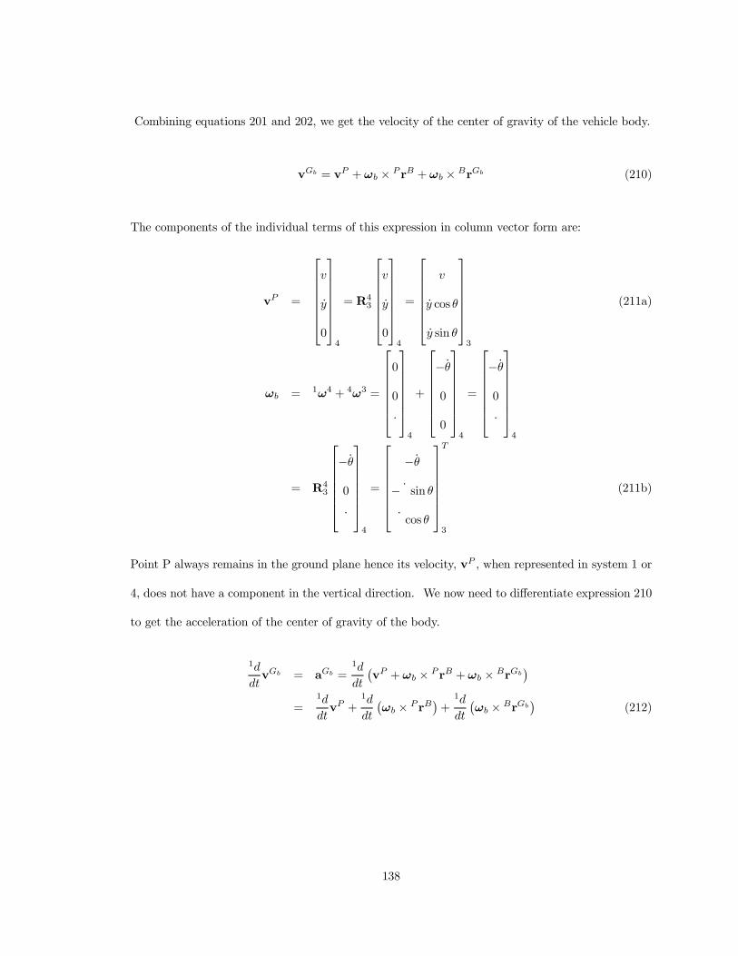
Combining equations 201 and 202, we get the velocity of the center of gravity of the vehicle body.
vGb = vP + !b £ P rB + !b £ BrGb (210)
The components of the individual terms of this expression in column vector form are:
vP =
26666664
v
_y
0
37777775
4
= R43
26666664
v
_y
0
37777775
4
=
26666664
v
_y cos θ
_y sin θ
37777775
3
(211a)
!b = 1!4 + 4!3 =
26666664
0
0
_ψ
37777775
4
+
26666664
¡ _θ
0
0
37777775
4
=
26666664
¡ _θ
0
_ψ
37777775
4
= R43
26666664
¡ _θ
0
_ψ
37777775
4
=
26666664
¡ _θ
¡ _ψ sin θ
_ψ cos θ
37777775
T
3
(211b)
Point P always remains in the ground plane hence its velocity, vP , when represented in system 1 or
4, does not have a component in the vertical direction. We now need to di¤erentiate expression 210
to get the acceleration of the center of gravity of the body.
1d
dtvGb = aGb =
1d
dt
¡vP + !b £ P rB + !b £ BrGb
¢
=1d
dtvP +
1d
dt
¡!b £ P rB
¢+
1d
dt
¡!b £ BrGb
¢(212)
138

We di¤erentiate each term to get:
1d
dtvP = aP =
4d
dtvP + 1!4 £ vP
=
26666664
_v
Äy
0
37777775
4
+
26666664
0
0
_ψ
37777775
4
£
26666664
v
_y
0
37777775
4
=
·_v ¡ _ψ _y v _ψ + Äy 0
¸T
4
(213)
To di¤erentiate the cross product terms, we again apply the transport theorem and the product rule
to get:
1d
dt
¡!b £ P rB
¢=
3d
dt
¡!b £ P rB
¢+ 1!3 £
¡!b £ P rB
¢
=3d
dt
¡!b £ P rB
¢+ !b £
¡!b £ P rB
¢(214)
Using the product rule, the …rst term on the right becomes:
3d
dt
¡!b £ P rB
¢= !b £
µ3d
dtP rB
¶+
µ3d
dt!b
¶£ P rB (215)
Using the fact that3ddt
P rB = 0,1ddt
¡!b £ P rB
¢becomes:
1d
dt
¡!b £ P rB
¢=
µ3d
dt!b
¶£ P rB + !b £
¡!b £ P rB
¢(216)
Explicitly, these terms are:
3d
dt!b =
26666664
¡Äθ
¡ (sin θ) Äψ ¡ _ψ _θ (cos θ)
(cos θ) Äψ ¡ _ψ _θ (sin θ)
37777775
3
(217)
139

µ3d
dt!b
¶£ P rB =
26666664
h³¡ (cos θ) _ψ _θ ¡ (sin θ) Äψ
´
hÄθ
0
37777775
3
=
26666664
h³¡ (cos θ) _ψ _θ ¡ (sin θ) Äψ
´
h (cos θ) Äθ
¡h (sin θ) Äθ
37777775
4
(218)
!b £¡!b £ P rB
¢=
26666664
¡h (cos θ) _ψ _θ
¡h (cos θ sin θ) _ψ2
¡ht2d ¡ h¡sin2 θ
¢_ψ2
37777775
3
=
26666664
¡h (cos θ) _ψ _θ
¡h (sin θ) _ψ2 ¡ h (sin θ) _θ
2
¡h (cos θ) _θ2
37777775
4
(219)
Equation 217 is found by di¤erentiation of the coordinates of !b when expressed in system 3. With
these de…nitions, equation 216 is:
1d
dt
¡!b £ P rB
¢=
26666664
¡h (cos θ) _ψ _θ + h³¡ (cos θ) _ψ _θ ¡ (sin θ) Äψ
´
h (cos θ) Äθ ¡ h (sin θ) _ψ2 ¡ h (sin θ) _θ
2
¡h (sin θ) Äθ ¡ h (cos θ) _θ2
37777775
4
(220)
We use the same process to get a similar expression for the last term of equation 212:
140

1d
dt
¡!b £ BrGb
¢=
26666664
¡2 (cos θ) _ψ _θgz ¡ _ψ2gx ¡ (sin θ) gz
Äψ
gxÄψ + (cos θ) gz
Äθ ¡ (sin θ) _ψ2gz ¡ (sin θ) _θ
2gz
¡ (sin θ) gzÄθ ¡ (cos θ) _θ
2gz
37777775
4
(221)
Combining equations 213, 220, and 221 we get the …nal expression for the acceleration of the center
of gravity of the vehicle body.
aGb =1d
dtvGb
=
26666664
_v ¡ _ψ _y ¡ _ψ2gx ¡ ξz
Äψ sin θ ¡ 2ξz_ψ _θ cos θ
v _ψ + Äy + gxÄψ + ξz
Äθ cos θ ¡ ξz_ψ2sin θ ¡ ξz
_θ2sin θ
¡ξz
³Äθ sin θ + _θ
2cos θ
´
37777775
4
(222)
ξz = h + gz (223)
C.1.1.1 Resultant Force. The A-arms of the vehicle chassis are approximated as
massless bodies and together with the forks and the vehicle body, form a parallelogram linkage, see
section V. This allows us to assume that they (the A-arms) work to create an independent force
and a couple acting on the vehicle body. In system 4, the resultant force is:
Fb = bPflw + bPfrw + bPrw + bFgrav
=
26666664
Pxflw
P yflw
P zflw
37777775
4
+
26666664
Pxfrw
Pyfrw
P zfrw
37777775
4
+
26666664
Pxrw
P yrw
P zrw
37777775
4
+
26666664
0
0
¡mbg
37777775
4
(224a)
C.1.1.1 Resultant Force.
mbaGb = bPflw + bPfrw + bPrw + bFgrav (225)
141

C.1.2 Moment Balance. The next step is to …nd an expression for equation 200 for the
vehicle body. To do this, we need an expression for Hb.
Hb = Ib!b =
26666664
Ixxb 0 ¡Ixz
b
0 Iyyb 0
¡Ixzb 0 Izz
b
37777775
3
¢
26666664
¡ _θ
¡ (sin θ) _ψ
(cos θ) _ψ
37777775
3
=
26666664
¡ (cos θ) _ψIxzb ¡ _θIxx
b
¡ (sin θ) _ψIyyb
_θIxzb + (cos θ) _ψIzz
b
37777775
3
(226)
The inertia tensor is de…ned with respect to the body …xed coordinates system 3 (see appendix A).
The axes of this system are not necessarily the principle axes. This is because there is only one plane
of symmetry, at the (x, z)3 plane. This plane of symmetry allows us to assume that the products
of inertia involving the y term are zero. If either of the (x, y)3 or (y, z)3 planes were also planes
of symmetry, then the system 3 axes would be principle axes and hence the quantity Ixzb would be
zero. We will, however, ultimately assume that the system 3 coordinates are su¢ciently close to
the principle axes. This will allow us to approximate Ixzb to be zero.
To di¤erentiate Hb in the inertial frame and …nd Euler’s equations of motion, we again use
the Transport Theorem ((34:pp. 117)).
1d
dtHb =
3d
dtHb + !b £ Hb (227)
3d
dtHb =
26666664
¡³(cos θ) Äψ ¡ _ψ _θ sin θ
´Ixzb ¡ ÄθIxx
b
¡³(sin θ) Äψ + _ψ _θ cos θ
´Iyyb
ÄθIxzb +
³(cos θ) Äψ ¡ _ψ _θ sin θ
´Izzb
37777775
3
(228)
142

!b £ Hb =
26666664
¡ (sin θ) _ψ _θIxzb + (sin θ) _ψ
2(cos θ) (¡Izz
b + Iyyb )
³_θ2 ¡
¡cos2 θ
¢_ψ2´
Ixzb + _θ (cos θ) _ψ (Izz
b ¡ Ixxb )
(Iyyb ¡ Ixx
b ) _ψ _θ sin θ ¡ (sin θ) _ψ2(cos θ) Ixz
b
37777775
3
(229)
Equation 227 then becomes:
1d
dtHb =
26666664
¡Ixzb (cos θ) Äψ ¡ ÄθIxx
b + (sin θ) _ψ2(cos θ) (¡Izz
b + Iyyb )
¡ξ1Iyyb +
h_θ2 ¡
¡cos2 θ
¢_ψ2iIxzb + _θ (cos θ) _ψ (Izz
b ¡ Ixxb )
ξ2Izzb + (Iyy
b ¡ Ixxb ) _ψ _θ sin θ +
³Äθ ¡ (sin θ) _ψ
2(cos θ)
´Ixzb
37777775
3
(230)
ξ1 = (sin θ) Äψ + _ψ _θ cos θ (231)
ξ2 = (cos θ) Äψ ¡ _ψ _θ sin θ (232)
C.1.2.1 Resultant Moment.
Mb = bMflw + bMfrw + bMrw ¡ Mδ +
BrGb £ bFgrav + BrGflw £ bPflw + BrGfrw £ bPfrw + BrGrw £ bPrw
=
26666664
Mxflw
0
0
37777775
6
+
26666664
Mxfrw
0
0
37777775
6
+
26666664
Mxrw
0
Mzrw
37777775
3
¡
26666664
0
0
Mδ
37777775
5
+BrGb £ bFgrav + BrGflw £ bPflw + BrGfrw £ bPfrw + BrGrw £ bPrw (233)
The moment is given in system 6 for simplicity sake. It becomes very complicated in system 3
and will require some simplifying assumptions before it can be used. This is postponed until the
equations for the wheels are developed.
143

C.1.2.2 Moment Balance Expression.
1d
dtHb = bMflw + bMfrw + bMrw ¡ Mδ
+BrGb £ Fgravb + BrGflw £ bPflw + BrGfrw £ bPfrw + BrGrw £ bPrw (234)
C.2 Front Wheels
The explicit expressions for the front wheels moment balance, become far too complex to be
usable for this paper. Some of the steps are listed however to illustrate both how the procedure
could be completed and why the simplifying assumptions need to be made.
C.2.1 Translational Balance. The translational balance, equation 199 for each of the front
wheels, is found in a similar manner as for the vehicle body by replacing BrGb with BrGflw and
BrGfrw . Restating equation 209b.
BrGflw =
26666664
lf
b2 cos θ
rfw + b2 sin θ ¡ h
37777775
3
, BrGfrw =
26666664
lf
¡ b2 cos θ
rfw ¡ b2 sin θ ¡ h
37777775
3
Starting with equation 201 for the front left wheel.
vGflw = vB + BvGflw , BvGflw =1d
dtBrGflw =
3d
dtBrGflw + !b £ BrGflw (235)
3d
dtBrGflw =
26666664
0
¡ b2_θ sin θ
b2_θ cos θ
37777775
3
(236)
144

In this case,3ddt
BrGflw is not zero because the con…guration of the vehicle is changing as it leans.
Combining this with equation 202 and again using the fact that3ddt
P rB = 0 we get:
vGflw = vP + !b £ P rB +3d
dtBrGflw + !b £ BrGflw (237)
Di¤erentiating this expression:
1d
dtvGflw = aGflw =
1d
dt
µvP + !b £ P rB +
3d
dtBrGflw + !b £ BrGflw
¶
=1d
dtvP +
1d
dt
¡!b £ P rB
¢+
1d
dt
µ3d
dtBrGflw
¶+
1d
dt
¡!b £ BrGflw
¢(238)
Next, we need expressions for the last 2 terms on the right.
1d
dt
µ3d
dtBrGflw
¶=
3d
dt
µ3d
dtBrGflw
¶+ !b £
3d
dtBrGflw (239)
3d
dt
µ3d
dtBrGflw
¶=
3d2
dt2BrGflw =
26666664
0
¡ b2
³_θ2sin θ + Äθ sin θ
´
b2
³¡ _θ
2sin θ + Äθ cos θ
´
37777775
3
(240)
!b £3d
dtBrGflw =
26666664
0
12_θ2b cos θ
12_θ2b sin θ
37777775
3
=
26666664
0
12_θ2b
0
37777775
4
(241)
1d
dt
¡!b £ BrGflw
¢=
3d
dt
¡!b £ BrGflw
¢+ !b £
¡!b £ BrGflw
¢(242)
3d
dt
¡!b £ BrGflw
¢= !b £
3d
dtBrGflw +
µ3d
dt!b
¶£ BrGflw (243)
145

Listed explicitly, these terms are:
1d
dt
¡!b £ BrGflw
¢= !b £
3d
dtBrGflw +
µ3d
dt!b
¶£ BrGflw + !b £
¡!b £ BrGflw
¢
µ3d
dt!b
¶£ BrGflw =
26666664
_θ (h ¡ rfw) cos θ _ψ ¡¡
12b ¡ (h ¡ rfw) sin θ
¢Äψ
³(cos θ) Äψ ¡ _ψ _θ sin θ
´lf ¡ Äθ
¡h ¡ rfw ¡ 1
2b sin θ¢
¡12Äθb cos θ +
³(sin θ) Äψ + _ψ _θ cos θ
´lf
37777775
3
=
26666664
_ψ _θ (h ¡ rfw) cos θ + Äψ (h ¡ rfw) sin θ ¡ 12Äψb
Äθ (rfw ¡ h) cos θ + lf Äψ
lf _ψ _θ ¡ Äθ¡
12b ¡ (h ¡ rfw) sin θ
¢
37777775
4
(244)
!b £¡!b £ BrGflw
¢=
26666664
ξ4_ψ _θ cos θ ¡ _ψ
2lf
³_ψ2ξ4 cos θ + lf _ψ _θ
´sin θ ¡ 1
2bξ3 cos θ
¡ξ4_ψ2cos2 θ ¡ _θ _ψ (cos θ) lf + ξ3
¡ξ4 ¡ 1
2 (sin θ) b¢
37777775
3
=
26666664
ξ4_ψ _θ cos θ ¡ _ψ
2lf
³_ψ2+ _θ
2´¡
h sin θ ¡ rfw ¡ 12b
¢
³¡ _θ
2rfw + _θ
2h´
cos θ ¡ lf _ψ _θ
37777775
4
(245)
ξ3 = _ψ2+ _θ
2(246)
ξ4 = h ¡ rfw (247)
146

Equation 238 then becomes:
aGflw =1d
dtvP +
1d
dt
¡!b £ P rB
¢+
3d2
dt2BrGflw + 2!b £
3d
dtBrGflw
+
µ3d
dt!b
¶£ BrGflw + !b £
¡!b £ BrGflw
¢(248)
Explicitly this is:
aGflw =
26666664
_v ¡ _ψ _y ¡ 2 _ψ _θ (cos θ) rfw ¡ (sin θ) Äψrfw ¡ 12Äψb ¡ _ψ
2lf
v _ψ + Äy + (cos θ) Äθrfw + lf Äψ ¡ _ψ2rfw sin θ ¡ (sin θ) _θ
2rfw ¡ 1
2_ψ2b
¡ (sin θ) Äθrfw ¡ (cos θ) _θ2rfw
37777775
4
(249)
Using the same process for the front right wheel, we get:
aGfrw =
26666664
_v ¡ _ψ _y ¡ 2 _ψ _θ (cos θ) rfw ¡ (sin θ) Äψrfw + 12Äψb ¡ _ψ
2lf
v _ψ + Äy + (cos θ) Äθrfw + lf Äψ ¡ _ψ2rfw sin θ ¡ (sin θ) _θ
2rfw + 1
2_ψ2b
¡ (sin θ) Äθrfw ¡ (cos θ) _θ2rfw
37777775
4
(250)
C.2.1.1 Resultant Force.
Ffw = fwPb + Fextfw
= fwPb +
26666664
0
Ff
Nfw ¡ mfwg
37777775
4
(251a)
147

C.2.1.1 Resultant Force.
mflwaGflw = flwPb + Fextflw (252a)
mfrwaGfrw = frwPb + Fextfrw (252b)
C.2.2 Moment Balance. Next, we need an expression for equation 200 for the front wheels.
It is this expression that becomes too complicated to use without any simplifying assumptions. For
completeness however, the steps are shown as to how this expression would be found. We start by
…nding !fw in the body …xed coordinate system 6.
!fw = 1!4 + 4!3 + 3!6 + !spinfw = !b + 3!6 + !spin
fw = 1!6 + !spinfw (253)
1!6 = !b +
26666664
0
0
_δ
37777775
6
=
26666664
¡ (cosβ cos δ) _θ ¡ (sin δ sin θ) _ψ + (sinβ cos δ cos θ) _ψ
(cosβ sin δ) _θ ¡ (cos δ sin θ) _ψ ¡ (sinβ sin δ cos θ) _ψ
(sinβ) _θ + (cosβ cos θ) _ψ + _δ
37777775
6
(254)
!spinfw =
26666664
0
ωspinfw
0
37777775
6
(255)
148

!fw =
26666664
¡ (cosβ cos δ) _θ ¡ (sin δ) _ψ sin θ + (sinβ cos δ) _ψ cos θ
ωspinfw + (cosβ sin δ) _θ ¡ (cos δ) _ψ sin θ ¡ (sinβ sin δ) _ψ cos θ
_δ + (sinβ) _θ + (cosβ) _ψ cos θ
37777775
6
(256)
Notice that ωspinfw > 0 when the vehicle has forward velocity. This is then used to …nd Hflw and
Hfrw.
Hfw = Ifw!fw
=
26666664
Ixxfw
³¡ (cosβ cos δ) _θ ¡ (sin δ) _ψ sin θ + (sinβ cos δ) _ψ cos θ
´
Iyyfw
³ωspin
fw + (cosβ sin δ) _θ ¡ (cos δ) _ψ sin θ ¡ (sinβ sin δ) _ψ cos θ´
Izzfw
³_δ + (sinβ) _θ + (cosβ) _ψ cos θ
´
37777775
6
(257)
The axes of system 6 are principle axes so the products of inertia are 0. The next step is to …nd
1ddt Hfw. As we did with the vehicle body, we use the transport theorem.
1d
dtHfw =
6d
dtHfw + 1!6 £ Hfw (258)
The cross product term involves the rotation of coordinate system 6. As we can see from the
expression for Hfw, the derivative and cross product terms in equation 258 will be quite complex.
For the sake of completeness, and that alone, they are listed here.
1!6 £ Hfw =
26666664
³Iyyfw ¡ Izz
fw
´Ax
7 ¡ IyyfwAx
6ωspinfw
³Ixxfw ¡ Izz
fw
´Ay
³Ixxfw ¡ Iyy
fw
´Az
9 + Iyyfw
³Az
7 + Az8
´ωspin
fw
37777775
6
(259)
149

Where the coe¢cients for the x term are:
Ax1 = cos δ sin θ sinβ +
¡1 ¡ 2 cos2 β
¢sin δ cos θ (260a)
Ax2 = cos δ sin θ + cos θ sinβ sin δ (260b)
Ax3 = ¡ cosβ sin δ (260c)
Ax4 = ¡ cosβ sinβ sin δ (260d)
Ax5 =
¡cos θ cos δ sin θ + cos2 θ sinβ sin δ
¢cosβ (260e)
Ax6 = _δ + _θ sinβ + _ψ cos θ cosβ (260f)
Ax7 =
³Ax
1_ψ _θ + Ax
2_ψ _δ + Ax
3_θ _δ + Ax
4_θ2
+ Ax5
_ψ2´
(260g)
For the y term:
Ay =³
_δ + _θ sinβ + _ψ cos θ cosβ´
¢³
_ψ cos θ cos δ sinβ ¡ _ψ sin θ sin δ ¡ _θ cosβ cos δ´
(261)
150

For the z term:
Az1 = cosβ sin θ ¡ 2 cos θ cosβ cos δ sinβ sin δ ¡ 2 cosβ cos2 δ sin θ (262a)
Az2 = cos2 β cos δ sin δ (262b)
Az3 = ¡ cos δ sin δ ¡ cos θ sin θ sinβ (262c)
Az4 = 2cos2 θ cos δ sin δ (262d)
Az5 = 2cos θ cos2 δ sin θ sinβ (262e)
Az6 = ¡ cos2 θ cos2 β cos δ sin δ (262f)
Az7 = ¡ _θ cosβ cos δ (262g)
Az8 = (cos θ cos δ sinβ ¡ sin θ sin δ) _ψ (262h)
Az9 =
³Az
1_θ _ψ + Az
2_θ2
+³Az
3 + Az4 + Az
5 + Az6
´_ψ2´
(262i)
The derivative term is:
6d
dtHfw =
26666664
Ixxfw
³Bx
1Äθ + Bx
2Äψ + Bx
3_θ _ψ + Bx
4_θ _δ + Bx
5_ψ _δ
´
Iyyfw
³_ωspinfw + By
1Äθ + By
2Äψ + By
3_θ _ψ + By
4_θ _δ + By
5_ψ _δ
´
Izzfw
³δ2d + Äθ sinβ + Äψ cos θ cosβ ¡ _ψ _θ sin θ cosβ
´
37777775
6
(263)
For the x term:
Bx1 = ¡ cosβ cos δ (264a)
Bx2 = sinβ cos δ cos θ ¡ sin δ sin θ (264b)
Bx3 = ¡ sin δ cos θ ¡ sinβ cos δ sin θ (264c)
Bx4 = cosβ sin δ (264d)
Bx5 = ¡ sin θ cos δ ¡ sinβ sin δ cos θ (264e)
151

For the y term:
By1 = Bx
4 = cosβ sin δ (265a)
By2 = Bx
5 = ¡ sin θ cos δ ¡ sinβ sin δ cos θ (265b)
By3 = ¡ cos θ cos δ + sinβ sin δ sin θ (265c)
By4 = ¡Bx
1 = cosβ cos δ (265d)
By5 = ¡Bx
2 = ¡ sinβ cos δ cos θ + sin δ sin θ (265e)
C.2.2.1 Simpli…ed Moment Balance. This form of the moment balance for the front
wheels is too cumbersome to be useful. There are 2 sources to the complexity. They are the
front wheels being steered and that they are steered about an axis that is not parallel to the k3
axis. To make the problem tractable, the approximation is made that the front wheels have zero
steering angle, δ ´ 0. The approximation is justi…ed partly because the mass of the front wheels
is only around 5% of the total mass of the vehicle in our case and because the equations would be
too complex without it. When this simpli…cation is made, coordinate system 6, the front wheels’
principle coordinate system, becomes the same as system 3. The angular momentum then becomes:
Hfw = Ifw!fw
152

!fw = 1!6 + !spinfw =
26666664
¡ _θ ¡ (sinβ) _δ
¡ (sin θ) _ψ
(cos θ) _ψ + (cosβ) _δ
37777775
3
+
26666664
0
ωspinfw
0
37777775
3
=
26666664
¡ _θ ¡ (sinβ) _δ
ωspinfw ¡ (sin θ) _ψ
(cos θ) _ψ + (cosβ) _δ
37777775
3
(266)
Hfw =
26666664
Ixxfw
³¡ _θ ¡ (sinβ) _δ
´
Iyyfw
³ωspin
fw ¡ (sin θ) _ψ´
Izzfw
³(cos θ) _ψ + (cosβ) _δ
´
37777775
3
(267)
Using this for equation 258 we get:
6d
dtHfw =
26666664
Ixxfw
³¡Äθ ¡ (sinβ) δ2d
´
Iyyfw
³_ωspinfw ¡ (sin θ) Äψ ¡ _ψ _θ (cos θ)
´
Izzfw
³(cos θ) Äψ ¡ _ψ _θ (sin θ) + (cosβ) Äδ
´
37777775
3
(268)
The cross product term is:
1!6 £ Hfw =
26666664
Cx1
³Iyyfw ¡ Izz
fw
´¡ ωspin
fw IyyfwCx
2
Cy³Izzfw ¡ Ixx
fw
´
Cz1
³Iyyfw ¡ Ixx
fw
´+ Cz
2
³Iyyfw ¡ Ixx
fw
´+ Cz
3 Iyyfw
37777775
3
(269)
For the x term:
Cx1 = _ψ (sin θ)
h(cosβ) _δ + (cos θ) _ψ
i(270a)
Cx2 = (cos θ) _ψ + (cosβ) _δ (270b)
153

For the y term:
Cy = _θ _ψ (cos θ) + _δ2(cosβ sinβ) + _θ _δ (cosβ) + _ψ _δ (cos θ sinβ) (271a)
For the z term:
Cz1 = _ψ _δ (sin θ sinβ) (272a)
Cz2 = _θ _ψ (sin θ) (272b)
Cz3 = ¡ωspin
fw
³_θ + (sinβ) _δ
´(272c)
C.2.2.2 Resultant Moment. The resultant moment is found about the center of
gravity of each front wheel. This is due to the moments from the vehicle body on the front wheels
and any moments due to external forces. The translational reactions from the vehicle body on the
front wheels as well as gravity are assumed to act at the center of gravity of the front wheels and so
have no a¤ect on the resultant moment.
Mfw = fwMb + rFfw £ Fextfw +
1
2Mδ (273)
Where:
Fextfw = Fext
fw ¡ Fgravfw =
26666664
0
Ff
Nfw
37777775
4
(274)
rFfw=
26666664
0
0
¡rfw
37777775
3
=
26666664
¡ (sinβ cos δ) rfw
(sinβ sin δ) rfw
¡ (cosβ) rfw
37777775
6
(275)
154

rFfw £ Fextfw =
2 6 6 6 6 6 6 4
(cos β) rfwFf cos θ cos δ ¡ (cos β) rfwNfw cos δ sin θ
(cos β) rfwFf sin δ cos θ + (cos β) rfwNfw sin θ sin δ
¡ (sin β) rfwFf cos θ + (sin β) rfwNfw sin θ
3 7 7 7 7 7 7 5
6
=
2 6 6 6 6 6 6 4
¡ (sin θ) Nfwrfw + (cos θ) Ff rfw
¡¡ cos2 β
¢ ¡¡2 sin2 δ
¢+ 1
¢
2 (cos δ cos θ cos β sin δ) Ff rfw
¡2¡sin2 δ
¢ Ff rfw cos θ cos β sin β
3 7 7 7 7 7 7 5
3
(276)
The cross product, k6, term matches Mtrail for reference (33) when rfw sin β = γ cos β.
t
Front Wheel
Steer Axis
γ
rfw
β
Figure C-1 Front wheel side view: trail schematic
The trail a¤ects and model dynamics are discussed in more detail the following references (7),
(12), (18:pp. 19), (23), (25), (28), (32), and (33).
155

C.2.2.3 Moment Balance Expression.
1d
dtHflw = flwMb + rFflw £ Fext
flw +1
2Mδ (277a)
1d
dtHfrw = frwMb + rFfrw £ Fext
frw +1
2Mδ (277b)
C.3 Rear Wheel
C.3.1 Translational Balance. We proceed as before. The relative position vector was
given in equation 209c.
BrGrw =
26666664
¡lr
0
rrw ¡ h
37777775
3
(278)
vGrw = vB + BvGrw , BvGrw =1d
dtBrGrw =
3d
dtBrGrw + !b £ BrGrw (279)
Since,3ddt
BrGrw =3ddt
P rB = 0 we get:
vGrw = vP + !b £ P rB + !b £ BrGrw (280)
Where we used equation 202. Again, the next step is to di¤erentiate this.
1d
dtvGrw = aGrw =
1d
dtvP +
1d
dt
¡!b £ P rB
¢+
1d
dt
¡!b £ BrGrw
¢(281)
156

The last term is found as we did before. Explicitly, it is:
1d
dt
¡!b £ BrGrw
¢=
26666664
_ψ2lr + ξ5
³(cos θ) 2 _ψ _θ + (sin θ) Äψ
´
¡ξ5
³Äθ ¡ (cos θ sin θ) _ψ
2´
¡ (cos θ) lr Äψ
ξ5
³_θ2
+¡sin2 θ
¢_ψ2´
¡ lr (sin θ) Äψ
37777775
3
(282)
=
26666664
_ψ2lr + ξ5
³2 (cos θ) _ψ _θ + (sin θ) Äψ
´
ξ5
³¡Äθ (cos θ) + (sin θ)
³_ψ2
+ _θ2´´
¡ lr Äψ
ξ5
³Äθ sin θ + _θ
2cos θ
´
37777775
4
(283)
ξ5 = h ¡ rrw (284)
Combining equations 213, 220, and 282 we get the acceleration of the rear wheel.
aGrw =
26666664
_v ¡ _ψ _y + _ψ2lr ¡ 2 (cos θ) _ψ _θrrw ¡ (sin θ) Äψrrw
³¡ _ψ
2 ¡ _θ2´
rrw sin θ + v _ψ + Äy + Äθ (cos θ) rrw ¡ lr Äψ
¡ (cos θ) _θ2rrw ¡ (sin θ) Äθrrw
37777775
4
(285)
C.3.1.1 Resultant Force.
Frw = rwPb + Fextrw = rwPb +
26666664
0
Fr
Nrw ¡ mrwg
37777775
4
(286)
C.3.1.2 Translational Balance Expression.
mrwaGrw = rwPb + Fextrw (287)
157

C.3.2 Moment Balance. The moment balance for the rear wheel is signi…cantly more
simple than that of the front wheels.
!fw = 1!4 + 4!3 + !spinrw = !b + !spin
rw = !b +
26666664
0
ωspinrw
0
37777775
3
=
26666664
¡ _θ
¡ _ψ sin θ
_ψ cos θ
37777775
3
+
26666664
0
ωspinrw
0
37777775
3
=
26666664
¡ _θ
¡ _ψ sin θ + ωspinrw
_ψ cos θ
37777775
3
(288)
The angular momentum Hrw is the product of the inertia tensor and the angular velocity in system
3. System 3 is the principle axis system so that the inertia tensor is again diagonal.
Hrw = Irw!rw =
26666664
¡Ixxrw
_θ
Iyyrw
³¡ _ψ sin θ + ωspin
rw
´
Izzrw
_ψ cos θ
37777775
3
(289)
Using the transport theorem for the time derivative of Hrw:
1d
dtHrw =
3d
dtHrw + !b £ Hrw (290)
3d
dtHrw =
26666664
¡Ixxrw
Äθ
Iyyrw
³¡ _ψ _θ cos θ ¡ Äψ sin θ + _ωspin
rw
´
Izzrw
³¡ _ψ _θ sin θ + Äψ cos θ
´
37777775
3
(291)
158

!b £ Hrw =
26666664
(¡Izzrw + Iyy
rw) (sin θ cos θ) _ψ2 ¡ _ψ (cos θ) Iyy
rwωspinrw
(¡Ixxrw + Izz
rw) (cos θ) _ψ _θ
(Iyyrw ¡ Ixx
rw) _θ _ψ sin θ ¡ _θIyyrwωspin
rw
37777775
3
(292)
Thus1ddt Hrw is:
1d
dtHrw =
26666664
¡Ixxrw
Äθ + (¡Izzrw + Iyy
rw) (sin θ cos θ) _ψ2 ¡ _ψ (cos θ) Iyy
rwωspinrw
Iyyrw
³¡ _ψ _θ cos θ ¡ Äψ sin θ + _ωspin
rw
´+ (¡Ixx
rw + Izzrw) (cos θ) _ψ _θ
Izzrw
³¡ _ψ _θ sin θ + Äψ cos θ
´+ (Iyy
rw ¡ Ixxrw) _θ _ψ sin θ ¡ _θIyy
rwωspinrw
37777775
3
(293)
C.3.2.1 Resultant Moment.
Mrw = rwMb + rFrw £ Fextrw (294)
Where:
Fextrw = Fext
rw ¡ Fgravrw =
26666664
0
Fr
Nrw
37777775
4
(295)
rFrw =
26666664
0
0
¡rrw
37777775
3
(296)
rFrw £ Fextrw =
26666664
rrw ((cos θ) Fr ¡ (sin θ)Nrw)
0
0
37777775
3
159

C.3.2.2 Moment Balance Expression.
1d
dtHrw = rwMb + rFrw £ Fext
rw (297)
C.4 Total Model
At this point, we have, 2 vector equations for each of the 4 bodies with the constraint equations:
fwPb = ¡bPfw (298a)
rwPb = ¡bPrw (298b)
fwMb = ¡bMfw (298c)
rwMb = ¡bMrw (298d)
We use these constraints to outline the procedure to derive the …nal equations of motion.
C.4.1 Translational Balance. Combining equations 225,252a,252b, and 287 we get the
overall translational balance expression, equation 299.
mbaGb + mflwaGflw + mfrwaGfrw + mrwaGrw = Fext
b + Fextflw + Fext
frw + Fextrw (299)
Explicitly, this simpli…es to equation 300.
m
26666664
_v ¡ _ψ _y ¡ hÄψ sin θ ¡ 2h _ψ _θ cos θ
v _ψ + Äy ¡ h _θ2sin θ + hÄθ cos θ ¡ h _ψ
2sin θ
¡h³Äθ sin θ + _θ
2cos θ
´
37777775
4
=
26666664
0
2Ff + Fr
2Nfw + Nrw ¡ mg
37777775
4
(300)
C.4.2 Moment Balance. This is where our ability to be explicit ends. The literal ex-
pressions for the total moment balance without any more simpli…cations becomes too complex to
160

calculate or manipulate explicitly. With the following de…nitions, we combine equations 234, 277a,
277b, and 297 to get
1d
dtH =
1d
dtHb + 2
1d
dtHfw +
1d
dtHrw
= BrGflw £ Fextflw + BrGfrw £ Fext
frw + BrGrw £ Fextrw
+BrGflw £ Fgravflw + BrGfrw £ Fgrav
frw + BrGrw £ Fgravrw
+rFfw £ Fextflw + rFfw £ Fext
frw + rFrw £ Fextrw
¡BrGflw £ mfwaGflw ¡ BrGfrw £ mfwaGfrw
¡BrGrw £ mrwaGrw (301)
1d
dtH =
¡rFfw + BrGflw
¢£ Fext
flw +¡rFfw + BrGfrw
¢£ Fext
frw
+¡rFrw + BrGrw
¢£ Fext
rw + BrGflw £ Fgravflw
+BrGfrw £ Fgravfrw + BrGrw £ Fgrav
rw
¡BrGflw £ mfwaGflw ¡ BrGfrw £ mfwaGfrw
¡BrGrw £ mrwaGrw (302)
The complication arises because of the front wheels’ principle coordinate system 6. We simplify
this expression by assuming that the mass of the wheels is negligible compared with the total mass
of the vehicle. When this is done, the last line of equation 302 disappears and we get equation 303.
1d
dtH =
1d
dtHb + 2
1d
dtHfw +
1d
dtHrw
=¡rFfw + BrGflw
¢£ Fext
flw +¡rFfw + BrGfrw
¢£ Fext
frw
+¡rFrw + BrGrw
¢£ Fext
rw + BrGb £ Fgravb
+BrGflw £ Fgravflw + BrGfrw £ Fgrav
frw + BrGrw £ Fgravrw (303)
161

An explicit expression for the left side of equation 303, is found by converting the expression
for1ddtHfw which is listed in system 6, to the system in which
1ddt Hb and
1ddtHrw are given, system 3.
By doing this, we get equation 304.
1d
dtH =
26666664
¡IxxÄθ + Dx1 (Iyy ¡ Izz) ¡ (cos θ) Ixz
bÄψ + Dx
5
¡Äψ (sin θ) Iyy + (cos θ) _θ _ψ (Izz ¡ Ixx ¡ Iyy) + Dy4
Äψ (cos θ) Izz + (sin θ) _θ _ψ (Iyy ¡ Ixx ¡ Izz) + Dz5
37777775
3
(304)
With the following de…nitions.
Dx1 = _ψ
2(cos θ sin θ) (305a)
Dx2 = (cosβ) _δωspin
fw Iyyfw + (sinβ) δ2dI
xxfw (305b)
Dx3 = 2 _ψ _δ (cosβ sin θ)
³Iyyfw ¡ Izz
fw
´(305c)
Dx4 = (cos θ) _ψ
³2ωspin
fw Iyyfw + ωspin
rw Iyyrw
´(305d)
Dx5 = ¡2Dx
2 + Dx3 ¡ Dx
4 (305e)
Dy1 = Ixz
b
³_θ2 ¡
¡cos2 θ
¢_ψ2´
+ 2ωsdfwIyy
fw + ωsdrwIyy
rw (306a)
Dy2 = _δ
2(cosβ sinβ)
¡Izzfw ¡ Ixx
fw
¢(306b)
Dy3 =
³(cosβ) _θ _δ + (cos θ sinβ) _ψ _δ
´ ¡Izzfw ¡ Ixx
fw
¢(306c)
Dy4 = Dy
1 + 2Dy2 + 2Dy
3 (306d)
162

Dz1 = Ixz
b
³Äθ ¡ (cos θ sin θ) _ψ
2´
(307a)
Dz2 = (cosβ) δ2dI
zzfw ¡ (sinβ) _δωspin
fw Iyyfw (307b)
Dz3 = _ψ _δ (sin θ sinβ)
³Iyyfw ¡ Ixx
fw
´(307c)
Dz4 = _θ
³2ωspin
fw Iyyfw + ωspin
rw Iyyrw
´(307d)
Dz5 = Dz
1 + 2Dz2 + 2Dz
3 ¡ Dz4 (307e)
These last three terms are due to the spinning and steering of the front wheel. Because the wheels
are signi…cantly lighter than the body, we neglect these terms when using the dynamic model. The
right side of equation 303 is listed explicitly as equations 308a and 308b.
¡rFfw + BrGflw
¢£ Fext
flw +¡rFfw + BrGfrw
¢£ Fext
frw +¡rFrw + BrGrw
¢£ Fext
rw
=
26666664
h (cos θ) (2Ff + Fr) ¡ h (sin θ) (2Nfw + Nrw)
(sin θ) (Frlr ¡ 2Ff lf ) + (cos θ) (lrNrw ¡ 2lfNfw)
(sin θ) (lrNrw ¡ 2lfNfw) + (cos θ) (2Ff lf ¡ Frlr)
37777775
3
(308a)
BrGb £ Fgravb + BrGflw £ Fgrav
flw + BrGfrw £ Fgravfrw + BrGrw £ Fgrav
rw = 0 (308b)
163

The …nal explicit expression for the moment balance is found by combining equations 304, 308a,
and 308b along with equations 305 through 307.
26666664
¡IxxÄθ + Dx1 (Iyy ¡ Izz) ¡ (cos θ) Ixz
bÄψ + Dx
5
¡Äψ (sin θ) Iyy + (cos θ) _θ _ψ (Izz ¡ Ixx ¡ Iyy) + Dy4
Äψ (cos θ) Izz + (sin θ) _θ _ψ (Iyy ¡ Ixx ¡ Izz) + Dz5
37777775
3
=
26666664
h (cos θ) (2Ff + Fr) ¡ h (sin θ) (2Nfw + Nrw)
(sin θ) (Frlr ¡ 2Ff lf ) + (cos θ) (lrNrw ¡ 2lfNfw)
(sin θ) (lrNrw ¡ 2lfNfw) + (cos θ) (2Ff lf ¡ Frlr)
37777775
3
(309)
Equations 300 and 309 describe the motion of the vehicle in terms of the state variables. The
state equation describing the front wheel angle, δ , which is one degree of freedom, comes from the
moment balance in the k6 direction of equation 258.
Izzfw
³δ2d + Äθ sinβ + Äψ cos θ cosβ ¡ _ψ _θ sin θ cosβ
´
+³Ixxfw ¡ Iyy
fw
´³Az
1_θ _ψ + Az
2_θ2+
³Az
3 + Az4 + Az
5 + Az6
´_ψ2´
+Iyyfw
³Az
7 + Az8
´ωspin
fw
= ¡ (sinβ) rfwFf cos θ + (sinβ) rfwNfw sin θ +1
2Mδ (310)
For our purposes, this equation is not important since there was too much friction in the motion of
the front wheels to be able to use Mδ as a control input. Instead, we used the front wheel angle, δ ,
from the position control command of the steering motor ampli…er to control δ directly.
C.4.3 Nonlinear Closed Form. We can now obtain a closed form, one that does not contain
the normal forces, Nn, with some manipulations and simpli…cations. We start by …nding the closed
form for the vehicle’s yaw motion by combining the scalar moment balance equations for the j3 and
164

k3 directions of equation 309 to obtain:
Äψ ((cos θ) Izz + (tan θ) (sin θ) Iyy)
=Dy
4
cos θsin θ ¡ Dz
5 + 2_θ _ψ (sin θ) (Izz ¡ Iyy)
+ (2Ff lf ¡ Frlr) ((tan θ) (sin θ) + (cos θ)) (311)
The closed form equation describing the vehicle’s tilt motion is found by combining the scalar
moment balance equation in the i3 direction of equation 309, with the scalar translational balance
equation in the k4 direction of equation 300.
Äθ¡¡Ixx ¡ h2m sin2 θ
¢
= h (cos θ) (2Ff + Fr) + h2m (cos θ sin θ) _θ2 ¡ mgh sin θ
¡ _ψ2(cos θ sin θ) (Iyy ¡ Izz) + (cos θ) Ixz
bÄψ ¡ Dx
5 (312)
let J = Ixx + h2m sin2 θ, then: (313)
Äθ =1
J
³mgh (sin θ) ¡ h2m (cos θ sin θ) _θ
2´
+1
J_ψ2(cos θ sin θ) (Iyy ¡ Izz)
¡ 1
J
³Ixzb
Äψ (cos θ) + Dx5 ¡ h (2Ff + Fr) (cos θ)
´(314)
Neglecting the product of inertia we get the nonlinear closed form equation of tilting motion.
Äθ =1
J
³mgh (sin θ) ¡ h2m (cos θ sin θ) _θ
2´
+1
J
³_ψ2(cos θ sin θ) (Iyy ¡ Izz) ¡ h (2Ff + Fr) (cos θ)
´
+1
JDx
5 (315)
165

The lateral translation equation is now found as:
Äy = ¡v _ψ ¡ 1
Jgh2m cos θ sin θ
+h _θ2µ
(sin θ) +1
Jh2m cos2 θ sin θ
¶
+h _ψ2µ
sin θ +1
J
¡cos2 θ sin θ
¢(Izz ¡ Iyy)
¶
+(2Ff + Fr)
µ1
Jh2 cos2 θ +
1
m
¶
¡ 1
JhDx
5 cos θ (316)
C.5 Model Linearization
In order to make the control design and simulation process more tractable (we are not concerned
with strict simulation accuracy), we linearize the above derived model. The equations are linearized
about the nominal values of θ = _θ = _ψ = _y = _δ = 0. When this is done, equations 300 and 309
respectively become: 26666664
m _v ¡ mhÄψθ
mv _ψ + mÄy + mhÄθ
¡mhÄθθ
37777775
4
=
26666664
0
2Ff + Fr
mg + 2Nfw + Nrw
37777775
4
(317)
26666664
¡IxxÄθ ¡ Ixzb
Äψ + Dx
¡ÄψθIyy + Dy
ÄψIzz + Ixzb
Äθ + Dz
37777775
3
=
26666664
h (2Ff + Fr) ¡ hθ (2Nfw + Nrw)
θ (Frlr ¡ 2Ff lf ) + (lrNrw ¡ 2lfNfw)
θ (lrNrw ¡ 2lfNfw) + (2Ff lf ¡ Frlr)
37777775
3
(318)
166

Dx = ¡2 (cosβ) _δωspinfw Iyy
fw ¡ 2 (sinβ) δ2dIxxfw ¡ _ψ
³2ωspin
fw Iyyfw + ωspin
rw Iyyrw
´(319a)
Dy = 2ωsdfwIyy
fw + ωsdrwIyy
rw (319b)
Dz = ¡2 (sinβ) _δωspinfw Iyy
fw + 2 (cosβ) δ2dIzzfw ¡ _θ
³2ωspin
fw Iyyfw + ωspin
rw Iyyrw
´(319c)
This yields the scalar equations:
m _v = mhÄψθ (320a)
mv _ψ + mÄy + mhÄθ = 2Ff + Fr (320b)
m³g ¡ hÄθθ
´= 2Nfw + Nrw (320c)
¡IxxÄθ ¡ Ixzb
Äψ + Dx = h (2Ff + Fr) ¡ hθ (2Nfw + Nrw) (320d)
¡ÄψθIyy + Dy = θ (Frlr ¡ 2Ff lf ) + (lrNrw ¡ 2lfNfw) (320e)
ÄψIzz + Ixzb
Äθ + Dz = θ (lrNrw ¡ 2lfNfw) + (2Ff lf ¡ Frlr) (320f)
Combining equations 320c and 320d gives equation 321.
IxxÄθ + Ixzb
Äψ ¡ Dx = ¡2hFf ¡ hFr + mghθ (321)
Equations 320e and 320f combine.
ÄψIzz + Ixzb
Äθ + Dz = θDy + 2Ff lf ¡ Frlr (322)
Using the approximation that the rotation of the wheels is related to the wheel radius and vehicle
velocity with together with equation 320a, the term involving Dy, is seen to be nonlinear in θ.
ÄψIzz + Ixzb
Äθ + Dz = 2Ff lf ¡ Frlr (323)
167

If we have an expression for the tire forces Ff , and Fr, in terms of the state variables, we will be in
a position to de…ne a closed form linear model that we can use to design our controller. The tire
forces were modeled linearly with tire slip angles. Figure 95 shows the important dimensions.
y
v
ψ
α
lf
lr
δ
..
Figure C-2 Top view schematic of vehicle with relavent slip angle velocities
tan α = _ y + lf
_ψ
v (324)
Since for moderate velocities, α is small, we can make the approximation that tan α ' α so that the
slip angle becomes:
δ ¡ _ y + lf _ψ
v (325)
For the rear wheel this is:
¡ _ y ¡ lr _ψ
v (326)
168

A camber e¤ect term was also included in the …nal expressions for the lateral tire forces.
Ff = Cf
Ãδ ¡ _y + lf _ψ
v
!+ λfθ (327)
Fr = Cr
á _y ¡ lr _ψ
v
!+ λrθ (328)
Cf and Cr were the proportionality gains from the slip angle and λf and λr are the proportionality
gains from the lean angle. The …nal linear model is now found using equations 320b, 321, and 323
while neglecting the product of inertia and the gyroscopic in‡uences of the tires.
Äψ =1
Izz(2Ff lf ¡ Frlr) (329)
Äθ =1
Ixx(mghθ ¡ 2hFf ¡ hFr) (330)
Äy = v _ψ ¡ hÄθ +1
m(2Ff + Fr)
= v _ψ ¡ gh2mθ
Ixx+ (2Ff + Fr)
µ1
m+
h2
Ixx
¶(331)
Using equations 327 and 328:
Äψ
=Crlr ¡ 2Cf lf
vIz_y ¡
2Cf l2f + Crl2r
vIz
_ψ
+1
Iz(2lfλf ¡ lrλr) θ + 2
lfIz
Cfδ (332)
Äθ
= h2Cf + Cr
Ixxv_y + h
2lfCf ¡ lrCr
Ixxv_ψ
+
µmgh
Ixx¡ h
Ixx(2λf + λr)
¶θ ¡ 2
h
IxxCfδ (333)
169

Let α = 1 + mh2
Ixx then:
Äy
= ¡ 1
mvα (2Cf + Cr) _y ¡
³v +
α
mv(2Cf lf ¡ Crlr)
´_ψ
+
µα
m(2λf + λr) ¡ mh2
Ixxg
¶θ + 2
α
mCfδ (334)
For consistency with other work we have done and to make cross-referencing easier, these equations
are re-ordered and listed in linear matrix form.
x =
·y _y ψ _ψ θ _θ
¸T
_x = Ax + Bδ (335)
A =
26666666666666666664
0 1 0 0 0 0
0 ¡ αmv (2Cf + Cr) 0 ¡
¡v + α
mv (2Cf lf ¡ Crlr)¢
αm (2λf + λr) ¡ mh2
Ixx g 0
0 0 0 1 0 0
0Crlr¡2Cf lf
vIz0 ¡2Cf l2f+Crl2r
vIz
1Iz
(2lfλf ¡ lrλr) 0
0 0 0 0 0 1
0 h2Cf +Cr
Ixxv 0 h2lfCf¡lrCr
IxxvmghIxx ¡ h
Ixx (2λf + λr) 0
37777777777777777775
(336)
B =
·0 2 α
mCf 0 2lfCf
Iz0 ¡ 2
IxhCf
¸T
(337)
The output of this state space depends on whether or not you can assume the driver’s intentions
known or not. In our case, we are not concerned with lateral control or global vehicle position but
only with tilting stabilization. In this case, the tilting is not dependent on the state variables y or
ψ so we can re-write these equations as:
x =
·_y _ψ θ _θ
¸T
(338)
170

A =
266666666664
¡ αmv (2Cf + Cr) ¡
¡v + α
mv (2Cf lf ¡ Crlr)¢
αm (2λf + λr) ¡ mh2
Ixx g 0
Crlr¡2Cf lfvIz
¡2Cf l2f +Crl2rvIz
1Iz
(2lfλf ¡ lrλr) 0
0 0 0 1
h2Cf +Cr
Ixxv h2lf Cf ¡lrCr
IxxvmghIxx ¡ h
Ixx (2λf + λr) 0
377777777775
(339)
B =
·2 α
mCf 2lfCf
Iz0 ¡ 2
IxhCf
¸T
(340)
With the output equation:
y = Cx =
26666664
0 1 0 0
0 0 1 0
0 0 0 1
37777775
x (341)
C.6 Error Coordinates
The last step is to derive a lateral mode error coordinate transformation similar to (8). The
coordinate transformations we used were:
Äe1 = Äy + v _ψ ¡ v _ψdes = Äy + v _e2 (342a)
_e1 = _y + vψ ¡ vψdes = _y + ve2 (342b)
e2 = ψ ¡ ψdes (342c)
e3 = θ ¡ θdes (342d)
Where the subscripted des terms are the properties of the vehicle trajectory the driver is trying to
follow. This trajectory can be parameterized by the maneuver curvature Cv, using the equations
developed in the section 2.2. By combining these transformation equations with equations 320b, 321,
and 323 and making the simplifying assumptions we used in the other models, we get the equations
for the regulator model laterally tracking a maneuver with a curvature, Cv. These coordinates are
171

useful for analyzing the …rst two control systems we designed which relied heavily on the lateral
control of the vehicle.
The assumptions are as such. The wheels are considered to have negligible mass and inertia
compared with the vehicle. This allows for the approximation, Dx ' Dz ' 0. Lastly, the axes
of coordinate system 3 are considered principle. When this is done, the product of inertia for the
vehicle body, Ixzb , is zero. Using these assumptions, we get equation 323 to be:
ÄψIzz = 2Ff lf ¡ Frlr (343)
In terms of error coordinates:
IzzÄe2 = 2Ff lf ¡ Frlr ¡ Izz Äψdes (344)
The term Äψdes is zero in a steady state turn but is certainly not zero in a transient maneuver. Next,
equation 321, with the simplifying assumptions becomes:
IxxÄθ = ¡2hFf ¡ hFr + mghθ (345)
Again, with error coordinates:
IxxÄe3 = ¡2hFf ¡ hFr + mgh (e3 + θdes) ¡ IxxÄθdes (346)
Lastly, we use equation 345 with equation 320b to get the lateral equation of motion.
mÄe1 = αFr + 2αFf ¡ mve2 ¡ mv _ψdes ¡ m2 h2
Ixxge3 ¡ m2 h2
Ixxgθdes (347)
172

Where we de…ned α = 1 + mh2
Ixx . Using equations 342a - 342d, equations 327 and 328 become:
Ff = Cf
0@δ ¡
( _e1 ¡ ve2) + lf³
_e2 + _ψdes
´
v
1A + λf (e3 ¡ θdes) (348)
Fr = Cr
0@¡
( _e1 ¡ ve2) ¡ lr³
_e2 + _ψdes
´
v
1A + λr (e3 ¡ θdes) (349)
We can now use equations 348 and 349 in the equations 344, 346, and 347.
Äe1 = ¡ α
mv(2Cf + Cr) _e1 +
α
m(2Cf + Cr) e2 +
³ α
mv(Crlr ¡ 2Cf lf ) ¡ v
´_e2
+³ α
m(2λf + λr) + g (1 ¡ α)
´e3 +
2α
mCfδ
+³ α
mv(Crlr ¡ 2Cf lf ) ¡ v
´_ψdes ¡
³ α
m(2λf + λr) ¡ g (1 ¡ α)
´θdes (350)
The yaw equation becomes:
Äe2 =1
vIzz(Crlr ¡ 2Cf lf ) _e1 +
1
Izz(2Cf lf ¡ Crlr) e2 ¡ 1
vIzz
¡2Cf l2f + Crl
2r
¢_e2
+1
Izz(2lfλf ¡ lrλr) e3 + 2Cf
lfIzz
δ ¡ 1
vIzz
¡2Cf l2f + Crl
2r
¢_ψdes
¡Äψdes +1
Izz(lrλr ¡ 2lfλf ) θdes (351)
Finally, the leaning equation becomes:
Äe3 =h
vIxx(2Cf + Cr) _e1 ¡ h
Ixx(2Cf + Cr) e2 +
h
vIxx(2Cf lf ¡ Crlr) _e2
+h
Ixx(mg ¡ 2λf ¡ λr) e3 ¡ 2h
Cf
Ixxδ
+h
vIxx(2Cf lf ¡ Crlr) _ψdes +
h
Ixx(gm + 2λf + λr) θdes ¡ Äθdes (352)
173

These transformations are valuable for designing an autonomous vehicle performing lateral as well
as tilt control. With this transformation, the driver will be laterally controlling the vehicle if the
error coordinates tend to zero, e1, e2, e3 ! 0.
174

References
1. Hibbard, R. and Karnopp, D., “The Dynamics of Small, Relatively Tall and Narrow Tilting Ground Vehicles”, ASME 1993, Advanced Automotive Technologies, DSC-Vol 52, 1993 pp. 397-417.
2. Hibbard, R. and Karnopp, D., (1993) “Methods of Controlling the Lean Angle of Tilting Vehicles”, ASME 1993, Advanced Automotive Technologies, DSC-Vol 52, pp. 311-320.
3. So, S. G., Karnopp, D., (1997) “Active Dual Mode Tilt Control for Narrow Ground Vehicles”, Vehicle System Dynamics, v. 27 1997, pp. 19-36.
4. Karnopp, D., Fang, C., (1992) “A Simple Model of Steering-Controlled Banking Vehicles”, ASME 1992, Transportation Systems, DSC-Vol 44, pp. 15-28.
5. So, S.G. and Karnopp, D., “Switching Strategies for Narrow Ground Vehicles with Dual Mode Automatic Tilt Control”, Int. J. of Vehicle Design v. 18 No. 5 (Special Issue), 1997, pp. 518 – 533.
6. Karnopp, D. Hibbard, R., (1992) “Optimum Roll Angle Behavior for Tilting Ground Vehicles”, ASME 1992, Transportation Systems, DSC-Vol 44, pp. 29-37.
7. Cossalter, V., Doria, A., Lot, R., (1999) “Steady Turning of Two-Wheeled Vehicles”, Vehicle System Dynamics, v. 31 1999, pp. 157-181.
8. Cossalter, V., Lio, M. D., Lot, R., Fabbri, L., “A General Method for the Evaluation of Vehicle Manoevrability with Special Emphasis on Motorcycles”, Vehicle System Dynamics, 31 1999, pp. 113-135.
9. Cossalter, V. and Lot, R., (2002) “A Motorcycle Multi-Body Model for Real Time Simulations Based on the Natural Coordinates Approach”, Vehicle System Dynamics, v. 37 No. 6 2002, pp. 423-447.
10. Lee, Allan Y., (1997) “Matching Vehicle Responses Using the Model-Following Control Method”, SAE SP-1228 Research into Vehicle Dynamics and Simulation, pp. 57-69.
11. Lee, A. Y., “Emulating the Lateral Dynamics of a Range of Vehicles Using a Four-Wheel-Steering Vehicle”, SAE 950304, 1995, pp. 11 – 22.
12. Nishimi, T., Aoki, A., and Katayama, T., “Analysis of Straight Running Stability of Motorcycles”, 10th International Technical Conference on Experimental Safety Vehicles, July 1985, pp. 1080 – 1094.
13. Aoki, A., “Experimental Study on Motorcycle Steering Performance”, SAE 790265, 1979, 16 pp.
14. Yuhara, N., Tajima, J., Sano, S., and Takimoto, S., “Steer-by-Wire-Oriented Steering System Design: Concept and Examination”, Vehicle System Dynamics suppl. 33, 1999, pp. 692 – 703.
15. Bundorf, R. T. and Le¤ert, R. L., “The Cornering Compliance Concept for Description of Vehicle Directional Control Properties”, SAE 760713, 1976, 14 pp.
16. Ryu, J. and Kim, H., “Virtual Environment for Developing Electronic Power Steering & Steer-by-Wire Systems”, Proceedings of the 1999IEEE/RSJ International Conference on Intelligent Robots and Systems, 1999, pp. 1374 – 1379.
17. Weir, D. H. and McRuer, D. T., “A Theory for Driver Steering Control of Motor Vehicles”, Highway Research Record No. 247, 1968, pp. 7 – 28.
175

18. Weir, D.H., and Zellner, J.W., “Lateral-Directional Motorcycle Dynamics and Rider Control”, SAE 780304, 1978 25 pp., (also in SP-428, pp. 7 – 31).
19. Zellner, J. W. and Weir, D. H., “Development of Handling Test Procedures for Motorcycles”, SAE 780313, 1978 (also in SP-428, pp. 91 – 100), 10 pp.
20. Weir, D. H. and Zellner, J. W., “Experimental Investigation of the Transient Behavior of Mo-torcycles”, SAE 790266, 1976, 17 pp.
21. Post, J. W., Burke, R. J., Drexel, M. V., and Robertson, J. D., “An Adaptive Control Model for Lateral Path Following with Closed-Loop Handling Simulations”, SAE 971061, 1997, pp. 217 – 231.
22. Rice, R. S., “Rider Skill In‡uences on Motorcycle Maneuvering”, SAE Transactions, v. 87 section 2, 1978, pp.1419 – 1430.
23. Sharp, R.S., “The Stability and Control of Motorcycles”, Journal of Mechanical Engineering Science v. 13 No. 5 1971, pp. 316 – 329.
24. Sharp, R. S., “The Dynamics of Single Track Vehicles”, Vehicle System Dynamics 5, 1975-1976, pp. 67 – 77.
25. Sharp, R. S., “Stability, Control and Steering Responses of Motorcycles”, Vehicle System Dynamics, v. 35 No. 4 – 5, 2001, pp. 291 – 318.
26. Sharp, R. S., “Research Note: The In‡uence of Frame Flexibility on the Lateral Stability of Motorcycles”, J. Mechanical Engineering Science, v. 16 No. 2, 1974, pp. 117 – 120.
27. Sharp, R. S., “A Review of Motorcycle Steering Behavior and Straight Line Stability Characteristics”, SAE 780303, 1978 (also in SP-428, pp. 1 – 6), 6 pp.
28. Sharp, R. S., “The Lateral Dynamics of Motorcycles and Bicycles”, Vehicle System Dynamics, 14 1985, pp. 265 – 283.
29. McKibben, J. S., “Motorcycle Dynamics-Fact, Fiction and Folklore”, SAE 780309, 1978 (also in SP-428, pp. 63 – 71), 9 pp.
30. Roe, G. E., Pickering, W. M., and Zinober, A., “The Oscillations of a Flexible Castor, and the E¤ect of Front Fork Flexibility on the Stability of Motorcycles”, SAE 780307, 1978 (also in SP-428, pp. 41 – 52), 12 pp.
31. Kane, T. R., The E¤ect of Frame Flexibility on High Speed Weave of Motorcycles”, SAE 780306, 1978 (also in SP-428, pp. 33 – 40), 8 pp.
32. Kane, T. R., “Fundamental Kinematical Relationships For Single-Track Vehicles”, International Journal of Mechanical Science v. 17, 1975, pp. 499 – 504
33. Rajamani, R., Gohl J., Alexander L., and Starr P., “Dynamics of Narrow Tilting Vehicles”, Mathematical and Computer Modelling of Dynamical Systems, Swets and Zeitlinger.
34. Baruh, Haim, Analytical Dynamics, McGraw-Hill 1999.
35. Shabana, Ahmed A., “Dynamics of Multibody Systems” 2nd ed., Cambridge University Press 1998.
36. Gillespie, Thomas D., “Fundamentals of Vehicle Dynamics”, SAE 1992.
37. Ogata, Katsuhiko, “Modern Control Engineering” 3rd ed., Prentice Hall 1997.
176

38. Franklin, Gene F., Powell, J. David, and Workman, Michael, “Digital Control of Dynamic Systems” 3rd ed., Addison Wesley 1998.
39. Beauchamp, K. G., Signal Processing Using Analog and Digital Techniques, John Wiley and Sons 1973.
40. Tewari, Ashish, Modern Control Design with Matlab and Simulink, John Wiley and Sons 2002.
41. Fitzpatrick, Patrick M., Advanced Calculus: A course in Mathematical Analysis, PWS Publishing Co. 1996.
42. “Motorcycle Safety”, NHTSA DOT HS 807 709, October1999.
43. Mercedes-Benz website, http://www.mercedes-benz.com/e/innovation/fmobil/f300_mobilitaet.htm, March 11, 2003.
44. Tilting Three-Wheelers reference website, http://www.maxmatic.com/ttw_index.htm, March 22, 2003.
45. Millennium Motorcycle’s website, http://members.iinet.net.au/126jsulman/tracer/, March 22, 2003.
177