development of a sun-tracker
TRANSCRIPT

UNIVERSIDADE FEDERAL DE VIÇOSA
CENTRO DE CIÊNCIAS EXATAS E TECNOLÓGICAS
DEPARTAMENTO DE ENGENHARIA ELÉTRICA
DEVELOPMENT OF A SUN-TRACKER
GABRIEL AKIRA GOMES RIBEIRO
VIÇOSA
MINAS GERAIS – BRAZIL
SEPTEMBER / 2012
GABRIEL AKIRA GOMES RIBEIRO
DEVELOPMENT OF A SUN-TRACKER
Final paper presented to the Department of Electrical
Engineering of the Center for Science and
Technology, Federal University of Viçosa, for
crediting the discipline ELT 490 - Monograph and
Seminary and partial fulfillment of the requirement
for the degree of Bachelor in Electrical Engineering.
Leader: Prof. Ms. Heverton Augusto Pereira.
VIÇOSA
MINAS GERAIS – BRAZIL
SEPTEMBER / 2012

3

4
GABRIEL AKIRA GOMES RIBEIRO
DEVELOPMENT OF A SUN-TRACKER
Final paper presented to the Department of Electrical Engineering of the Center for Science
and Technology, Federal University of Viçosa, for crediting the discipline ELT 490 -
Monograph and Seminary and partial fulfillment of the requirement for the degree of
Bachelor in Electrical Engineering.
COMMISSION EXAMINER
Prof. M.Sc. Heverton Augusto Pereira - Orientador
Departamento de Engenharia Elétrica
Universidade Federal de Viçosa
Prof.ª – D. Sc. Joyce Correna Carlo - Membro
Departamento de Arquitetura e Urbanismo
Universidade Federal de Viçosa
Prof. ª – D. Sc. Olga Moraes Toledo - Membro
Coordenação de Eletrotécnica / Automação Industrial
CEFET-MG campus III - Leopoldina
M.Sc. – José Vitor Nicácio – Membro
Doutorando no Departamento de Engenharia Agrícola
Universidade Federal de Viçosa

5
“To my dear family Dida, Zene and Sâmia”
6
Acknowledgment
Agradeço a Deus, fonte de toda sabedoria e luz, sempre presente em minha vida. Aos
meus pais Djalma e Maria Zene pelo carinho, apoio incondicional, palavras de sabedoria e por
sempre batalharem em prol dos meus estudos acreditando em mais esta conquista. A minha
irmã Sâmia, pela amizade e companheirismo durante esses anos. Ao meu tio Edson, por
sempre me auxiliar antes e durante a graduação, me mostrando o melhor caminho a seguir. Ao
Afrânio, pela amizade e companheirismo durante o tempo de república.
Ao professor Heverton, pela amizade, orientação, motivação e principalmente por sempre
acreditar na conclusão deste trabalho. A minha equipe do GESEP, pela troca de experiências e
sempre me apoiarem no meu projeto, especialmente ao Lucas Queiroz, Guilherme Vianna e
Guilherme Martins pelo auxílio durante esse trabalho. Aos professores do Departamento de
Engenharia Elétrica pelos ensinamentos e por me guiarem durante esta caminhada.
A todos os meus colegas da Engenharia Elétrica e amigos de Viçosa que dividiram
momentos de muita alegria e fizeram valer cada minuto nesta cidade maravilhosa. A toda
minha família e amigos de Araçuaí pela torcida, diálogo e incentivo durante estes anos, o meu
MUITO OBRIGADO!!

7
“The good idea is not discovered or undiscovered, it comes, it happens.”
Johan Galtung

8
Abstract
The power generated by a solar panel is directly related to the level of solar radiation
falling on it. The most advanced solar panels convert 20% to 25% of irradiance energy,
besides, a steady panel has a decrease in its production and in certain moments of the day it
doesn't produce. Therefore, it is necessary get more radiation to increase the generated power
by the panel and a system able to follow the sun's movement could improve efficiency in this
point. But the cost is an important variable to consider due to the enhancement of the final
system This paper presents a study and construction of a prototype for solar tracking during
the day in order to increase the power generated by the panel. The main objectives were to
build a simplified, robust and low cost of production and marketing potential on a large scale.
The tests showed an increase of 12 % to 18 % of the energy produced.

9
List of Figures
Figure 1 - Evolution of global cumulative installed capacity 2000-2011 (MW) [1]. .............. 14 Figure 2 - Variation of solar radiation incidence in Brazil [2]. ................................................ 15 Figure 3 – Pulse width modulation [5]. .................................................................................... 17 Figure 4 – Buck converter [5]. ................................................................................................. 17
Figure 5 - Boost converter [5]. ................................................................................................. 17
Figure 6 – The sun’s position can be described by its altitude angle β and its azimuth angle
[8]. .................................................................................................................................... 18 Figure 7 –A south-facing collector tipped up to an angle equal to its latitude angle [8]. ........ 19
Figure 8 - Parts of one-axis sun tracker [12]. ........................................................................... 20 Figure 9 - One-axis sun tracker [13]. ....................................................................................... 20 Figure 10 - Two-axis sun tracker [12]. ..................................................................................... 20
Figure 11 - Sample two-axis sun tracker [14]. ......................................................................... 20 Figure 12 – Parts of two-axis sun tracker [15]. ........................................................................ 20 Figure 13 - Variation of solar angles during the year for Viçosa-MG. .................................... 23 Figure 14 – Parts of prototype. ................................................................................................. 24 Figure 15 - Tilt adjustment. ...................................................................................................... 24
Figure 16 – Prototype with the motor and fixed on wood support. ......................................... 25
Figure 17 – Motor and gear system. ......................................................................................... 25 Figure 18 – Drive control. ........................................................................................................ 26 Figure 19 – Built control circuit. .............................................................................................. 26
Figure 20 – Box built. .............................................................................................................. 26 Figure 21 – Initial message. ..................................................................................................... 27
Figure 22 – Timer. .................................................................................................................... 27 Figure 23 – Data acquisition. ................................................................................................... 28
Figure 24 – Current sensor circuit. ........................................................................................... 28 Figure 25 – Panels under the same conditions. ........................................................................ 29
Figure 26 – Panels with same tilt. ............................................................................................ 29 Figure 27 – Build System. ........................................................................................................ 29 Figure 28 – Panel in same conditions. ...................................................................................... 31
Figure 29 – Voltage and current in August 20. ........................................................................ 31 Figure 30 – Power Track x Static System in August 20. ......................................................... 31
Figure 31 – Voltage and current in August 21. ........................................................................ 32 Figure 32 – Power Track x Static System in August 21. ......................................................... 32
Figure 33 – Voltage and current in August 22. ........................................................................ 32 Figure 34 – Power Track x Static System in August 22. ......................................................... 32 Figure 35 – Power gain percentage in comparison to the panel nominal power for August
20th. .................................................................................................................................. 33
Figure 36 – Power gain percentage in comparison to the panel nominal power for August
21st. .................................................................................................................................. 33 Figure 37 – Power gain percentage in comparison to the panel nominal power for August
22nd. ................................................................................................................................. 33 Figure 36 – Power Track x Static System in July 29. .............................................................. 38 Figure 37 – Power Track x Static System at the night in August 19. ...................................... 39

10

11
List of Tables
Table 1 – Current Sensor Specifications [22] .......................................................................... 28 Table 2 – Panel Technnical Features ........................................................................................ 29 Table 3 – Experimental conditions ........................................................................................... 30 Table 4 – Average Power During conditions ........................................................................... 33
12
SUMMARY
1. Introduction and Objective ............................................................................................... 13 2. Literature Review ............................................................................................................. 14
2.1. Perspective of Solar Energy in the world ................................................................. 14 2.2. Solar Energy in Brazil .............................................................................................. 15 2.3. Types of PV Systems ............................................................................................... 16 2.4. Static Converters ...................................................................................................... 16 2.5. Sun Tracking ............................................................................................................ 17
3. Metodology ...................................................................................................................... 23 3.1. Study of the Sun ....................................................................................................... 23 3.2. Building the prototype .............................................................................................. 24 3.3. Motor ........................................................................................................................ 25 3.4. Drive and control strategy ........................................................................................ 26
3.4.1. Drive control .................................................................................................... 26 3.4.2. Control strategy ................................................................................................ 27
3.5. System data acquisition ............................................................................................ 27 3.6. Complete system ...................................................................................................... 28 3.7. Weather conditions ................................................................................................... 30
4. Results .............................................................................................................................. 31
5. Conclusion ........................................................................................................................ 35 Bibliography ............................................................................................................................. 36 Appendix A .............................................................................................................................. 38
Appendix B .............................................................................................................................. 40

13
1. Introduction and Objective
The increase in energy demand together with the appeal for the use of less polluting
sources lead research centers to seek new forms of energy production. One is the photovoltaic
solar energy which appears as very promising renewable resource, it depends on the sun that
is an inexhaustible resource of light.
Solar energy reaches the Earth in the thermal and lighting forms. However, it does not
reach uniformly throughout its surface. It depends on the latitude, the season and weather
conditions such as cloudiness and relative humidity.
In this context it is necessary to increase the power generated by the solar panel. An
alternative and low cost is the use of structures that follow the sun. Thus it is possible to vary
the position of the solar panel during the day and to increase the intensity of received rays on
its surface. This is an alternative for projects to supply isolated locations.
One strategy is to move the structure based on the movement of the sun during the day
eliminating the use of sensors. In this case, variation of the sun angles during the day is
evaluated.
In order to build the solar tracker it was necessary to evaluate the kind of material
structure, a motor torque and ensures precision and control system effectively. In this study, a
stepper motor controlled by a PIC microcontroller was used.
The main objective of this work is to study and build a low cost sun tracker and compare
the power generated with a static panel.
The development of this work provided the following publication:
1. A Low-Cost Prototype for Sun Tracking. 10th
IEEE/IAS International Conference on
Industry Applications, 2012, Fortaleza, Brazil.
The organization of this work was done as follows: Literature Review (Chapter 2),
Methodology (Chapter 3) Experimental results (Chapter 4) and Conclusion (Chapter 5).
14
2. Literature Review
2.1. Perspective of Solar Energy in the world
In the last years, PV technology has shown the potential to become a major source of
power generation for the world with robust and continuous growth. PV is now, behind hydro
and wind power, the third most important renewable energy in terms of globally installed
capacity [1].
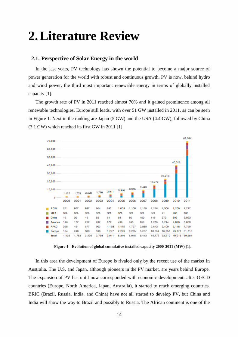
The growth rate of PV in 2011 reached almost 70% and it gained prominence among all
renewable technologies. Europe still leads, with over 51 GW installed in 2011, as can be seen
in Figure 1. Next in the ranking are Japan (5 GW) and the USA (4.4 GW), followed by China
(3.1 GW) which reached its first GW in 2011 [1].
Figure 1 - Evolution of global cumulative installed capacity 2000-2011 (MW) [1].
In this area the development of Europe is rivaled only by the recent use of the market in
Australia. The U.S. and Japan, although pioneers in the PV market, are years behind Europe.
The expansion of PV has until now corresponded with economic development: after OECD
countries (Europe, North America, Japan, Australia), it started to reach emerging countries.
BRIC (Brazil, Russia, India, and China) have not all started to develop PV, but China and
India will show the way to Brazil and possibly to Russia. The African continent is one of the

15
last of the list of recent development, although there is some potential for short-term in South
Africa [1].
2.2. Solar Energy in Brazil
As with the winds, Brazil is privileged in terms of solar radiation. The Northeast has
radiation comparable to the best parts of the world as the city of Dongola, in the desert of
Sudan and the region of Dagget, in the Mojave Desert, California. Figure 2 can be seen as
solar radiation varies in Brazil [2].
Figure 2 - Variation of solar radiation incidence in Brazil [2].
Currently, there are several projects using solar energy in Brazil, mainly for the attend
isolated communities of energy networks and regional development. The main types of
projects are: pumping water for domestic supply, irrigation and fish farming; lighting;
institutional buildings, such as electrification of schools, health centers and community
centers; dwellings [3].
The Brazilian National Electric Energy Agency was expected to introduce two regulations
in 2012 designed to promote the deployment of solar power in Brazil. One of the regulations
has introduced in April 2012 a net-metering system for micro generation up to 100 kW and
for mini systems up to 1 MW. The other regulation should provide an 80% tax break to
utilities companies that purchase electricity generated by large-scale solar parks (for systems
16
up to 30 MW). The first 1 MW plant was commissioned in 2011 and could have been
expanded if the regulation were consolidated. With a growing demand for electricity in the
country and good incidence of radiation, the development of PV systems is simply a question
of adequate regulation and awareness. The market can reach more than 1 GW by 2016 [1].
It can see that solar energy is not deeply explored in Brazil and according to [2] the total
installed capacity in the country is still very small beside its potential. This is because to the
country has enough water resources, resulting in investment in electricity generation from
hydroelectric plants. But this concept is already changing mainly because the cost, time and
environmental impacts on building hydroelectric power plants. And there are isolated places,
far from the grid, where the photovoltaic generation becomes viable, since it does not require
the implementation of transmission lines to reach these communities.
2.3. Types of PV Systems
Photovoltaic systems can be ranked into three main categories: isolated, grid connected or
hybrid. Each one may have different complexity depending on the application and the specific
constraints of each project.
The isolated systems are typically used in regions where the grid is not accessible. They
may not use or storage of energy through batteries, feeding a DC load or AC load using an
inverter [4].
In grid connect the PV array represents an additional source for a large electrical system to
which it is connected. Usually, it does not use energy storage, because all the power generated
is delivered to the network instantly. Installations of this type are becoming increasingly
popular in many European countries, Japan, USA and more recently in Brazil. The powers
range from a few kWp installed in residential facilities, until a few MWp in systems operated
by large companies [4].
Hybrid systems are those where more than one way of generating energy is available, for
example diesel generator, wind turbines and photovoltaic modules. These are more complex
and require a type of control can integrate the various generators optimizing the operation to
the user [4].
2.4. Static Converters
The output voltage generated in the panels is still, depending on the application, is
required to regulate the inverter output voltage. To achieve it, it can be used DC-DC
converters buck or boost. DC-DC converters are used for transferring electrical energy from a
17
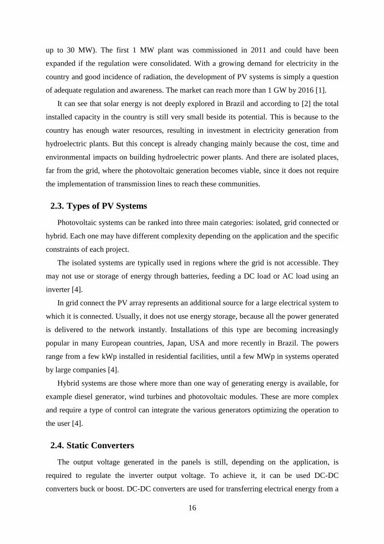
DC source into another DC source. These converters are widely used in regulated switching
power supplies and DC motor drive applications. The method used to control the output
voltage is called a pulse width modulation (PWM) and changes the duty cycle D which is the
ratio between the on-time key and the total period (TON + TOF) as can be seen in Figure 3
[5].
Figure 3 – Pulse width modulation [5].
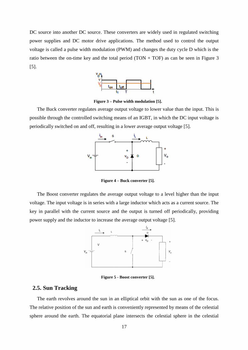
The Buck converter regulates average output voltage to lower value than the input. This is
possible through the controlled switching means of an IGBT, in which the DC input voltage is
periodically switched on and off, resulting in a lower average output voltage [5].
Figure 4 – Buck converter [5].
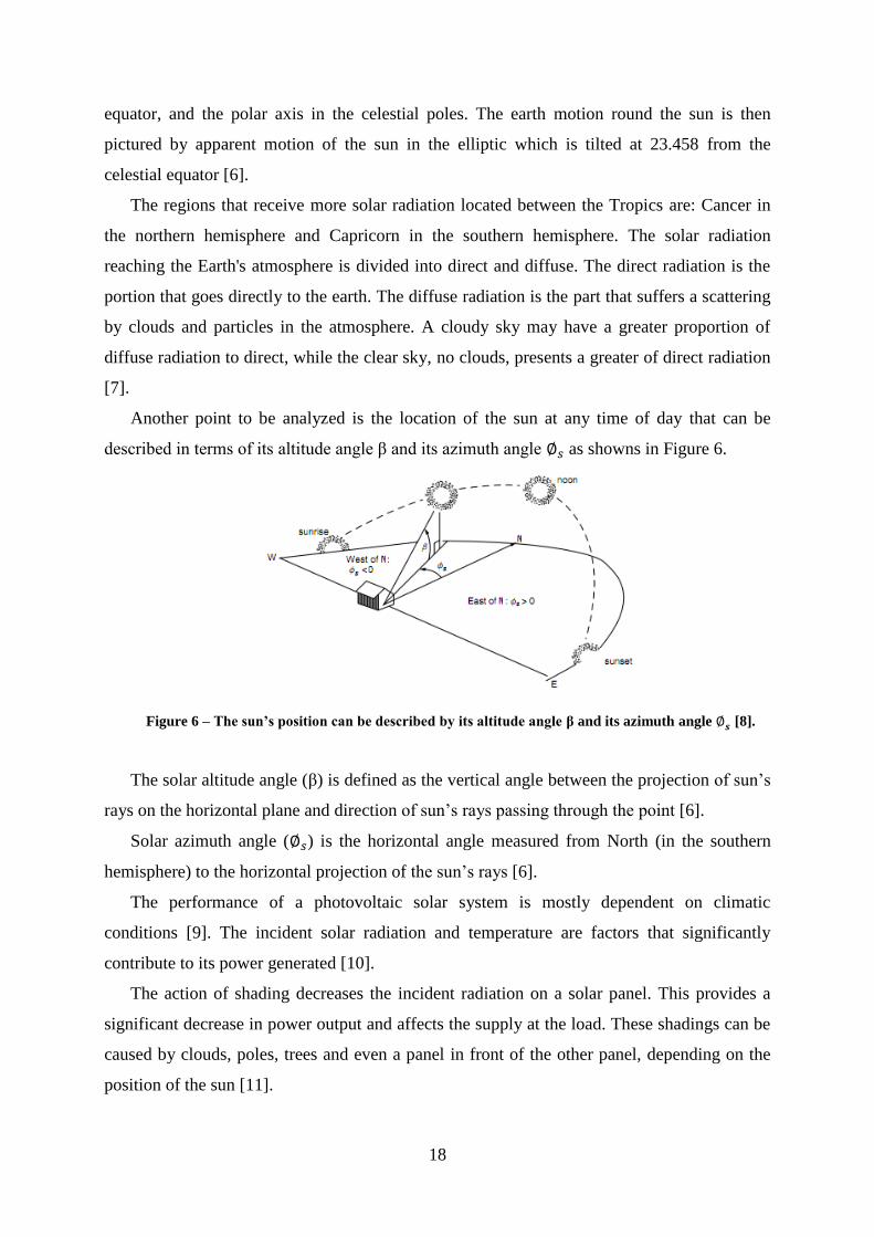
The Boost converter regulates the average output voltage to a level higher than the input
voltage. The input voltage is in series with a large inductor which acts as a current source. The
key in parallel with the current source and the output is turned off periodically, providing
power supply and the inductor to increase the average output voltage [5].
Figure 5 - Boost converter [5].
2.5. Sun Tracking
The earth revolves around the sun in an elliptical orbit with the sun as one of the focus.
The relative position of the sun and earth is conveniently represented by means of the celestial
sphere around the earth. The equatorial plane intersects the celestial sphere in the celestial
18
equator, and the polar axis in the celestial poles. The earth motion round the sun is then
pictured by apparent motion of the sun in the elliptic which is tilted at 23.458 from the
celestial equator [6].
The regions that receive more solar radiation located between the Tropics are: Cancer in
the northern hemisphere and Capricorn in the southern hemisphere. The solar radiation
reaching the Earth's atmosphere is divided into direct and diffuse. The direct radiation is the
portion that goes directly to the earth. The diffuse radiation is the part that suffers a scattering
by clouds and particles in the atmosphere. A cloudy sky may have a greater proportion of
diffuse radiation to direct, while the clear sky, no clouds, presents a greater of direct radiation
[7].
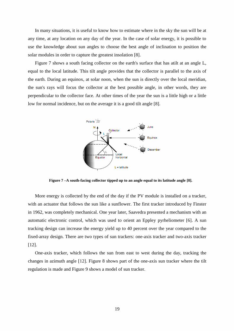
Another point to be analyzed is the location of the sun at any time of day that can be
described in terms of its altitude angle β and its azimuth angle as showns in Figure 6.
Figure 6 – The sun’s position can be described by its altitude angle β and its azimuth angle [8].
The solar altitude angle (β) is defined as the vertical angle between the projection of sun’s
rays on the horizontal plane and direction of sun’s rays passing through the point [6].
Solar azimuth angle ( ) is the horizontal angle measured from North (in the southern
hemisphere) to the horizontal projection of the sun’s rays [6].
The performance of a photovoltaic solar system is mostly dependent on climatic
conditions [9]. The incident solar radiation and temperature are factors that significantly
contribute to its power generated [10].
The action of shading decreases the incident radiation on a solar panel. This provides a
significant decrease in power output and affects the supply at the load. These shadings can be
caused by clouds, poles, trees and even a panel in front of the other panel, depending on the
position of the sun [11].
19
In many situations, it is useful to know how to estimate where in the sky the sun will be at
any time, at any location on any day of the year. In the case of solar energy, it is possible to
use the knowledge about sun angles to choose the best angle of inclination to position the
solar modules in order to capture the greatest insolation [8].
Figure 7 shows a south facing collector on the earth's surface that has atilt at an angle L,
equal to the local latitude. This tilt angle provides that the collector is parallel to the axis of
the earth. During an equinox, at solar noon, when the sun is directly over the local meridian,
the sun's rays will focus the collector at the best possible angle, in other words, they are
perpendicular to the collector face. At other times of the year the sun is a little high or a little
low for normal incidence, but on the average it is a good tilt angle [8].
Figure 7 –A south-facing collector tipped up to an angle equal to its latitude angle [8].
More energy is collected by the end of the day if the PV module is installed on a tracker,
with an actuator that follows the sun like a sunflower. The first tracker introduced by Finster
in 1962, was completely mechanical. One year later, Saavedra presented a mechanism with an
automatic electronic control, which was used to orient an Eppley pyrheliometer [6]. A sun
tracking design can increase the energy yield up to 40 percent over the year compared to the
fixed-array design. There are two types of sun trackers: one-axis tracker and two-axis tracker
[12].
One-axis tracker, which follows the sun from east to west during the day, tracking the
changes in azimuth angle [12]. Figure 8 shows part of the one-axis sun tracker where the tilt
regulation is made and Figure 9 shows a model of sun tracker.
20
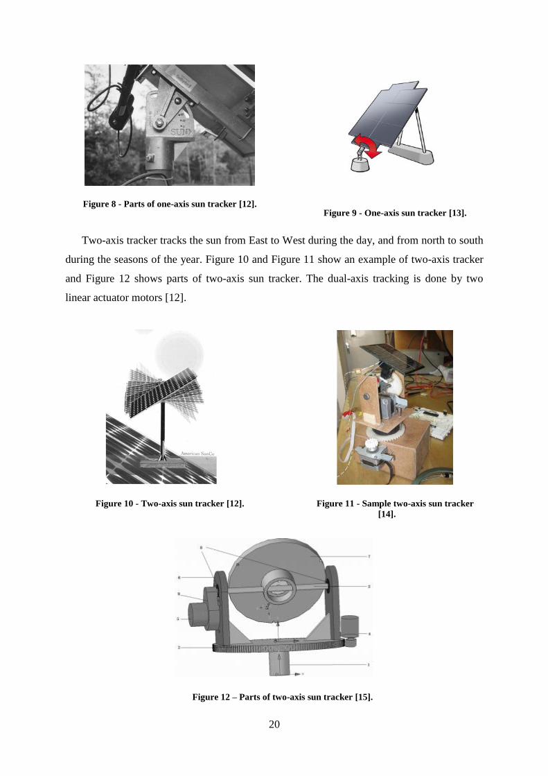
Figure 8 - Parts of one-axis sun tracker [12].
Figure 9 - One-axis sun tracker [13].
Two-axis tracker tracks the sun from East to West during the day, and from north to south
during the seasons of the year. Figure 10 and Figure 11 show an example of two-axis tracker
and Figure 12 shows parts of two-axis sun tracker. The dual-axis tracking is done by two
linear actuator motors [12].
Figure 10 - Two-axis sun tracker [12].
Figure 11 - Sample two-axis sun tracker
[14].
Figure 12 – Parts of two-axis sun tracker [15].

21
In [16] are compared results of a water pumping system driven by static, tracking and
tracking with concentration PVs in Recife (PE-Brazil) for one day. The PV generator consists
of four cavities and two PV modules tracking along its North–South axis, tilted at an angle of
20° towards the north. The advantage in terms of solar radiation, for tracking collectors is
equal to 1.23 and for concentrating collectors, is equal to 1.74. Those values for water volume
are 1.41 and 2.49 respectively.
Tomson compare the performance of PV modules with daily two-positional tracking. The
symmetrical and asymmetrical positions about the North–South axis are analyzed,
corresponding to the positions of sun in the morning and in the afternoon. According to this,
the effect of different tilt angles, initial tilt angle, initial azimuth, and azimuth angle of the
deflected plane on the daily and seasonal gain were evaluated. Results show that energy was
increase by 10–20% over the yield from a fixed south-facing collector tilted at an optimal
angle [17].
Michaelides studied the thermal performance and effective cost of thermosyphon solar
water heaters with different solar collector tracking modes under the weather and
socioeconomic conditions of Nicosia (Cyprus) and Athens (Greece). He compare the system
using the TRNSYS simulation program in four ways: fixed at 40° from the horizontal, the
single-axis tracking with vertical axis, fixed slope and variable azimuth and the seasonal
tracking mode where the collector slope is changed twice per year. The simulation results
showed that the best thermal performance was obtained with the single-axis tracking. In
Nicosia, the annual solar radiation with this mode was 87.6% compared to 81.6% with the
seasonal mode and to 79.7% with the fixed surface mode, while the corresponding figures for
Athens were 81.4%, 76.2% and 74.4%, respectively. From the economic point of view, the
fixed surface mode was found to be the most cost effective [18].
Farzin show in [14] a sample biaxial sun tracker with three algorithms of control from step
motors. The first algorithm proposes moving the structure in circular coordinates in the small
ranges and finding the point with the best voltage. The second algorithm finds the tilt of the
voltage and use it to find its way. Third algorithm is similar to second but use it to find some
appropriate points that are distinctly in different times.
Chen compares the solar irradiation for fixed bracket and uniaxial automatic solar
tracking. The system was produced by Kunming green electrical science and technology Ltd,
its name is Rack Sun. There were made three days of test with good weather conditions to

22
show that the system proposed can improve electricity quantity of solar PV system to 25~28%
[19].
Ponniran designed the single axis sun tracking system for residential usage and compared
it to static solar panel. It was used the microcontroller PIC16F877A and the control is based
in signals from the two different Light Dependent Resistor (LDR). The results show that the
system allows a considerable gain of energy during the day mainly in the morning [20].
23
3. Metodology
The purpose of this study was to build a solar tracker easily controlled, low cost, capable
of tracking the sun and increase the power available in the system. Based on this, it was
decided to study how the sun focus on the earth during each month of the year. Build a simple
prototype with resistant materials able to give support to the solar panel. In the end it was
define the drive and the control strategy based on studies of movement of the sun.
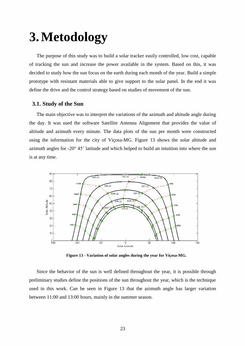
3.1. Study of the Sun
The main objective was to interpret the variations of the azimuth and altitude angle during
the day. It was used the software Satellite Antenna Alignment that provides the value of
altitude and azimuth every minute. The data plots of the sun per month were constructed
using the information for the city of Viçosa-MG. Figure 13 shows the solar altitude and
azimuth angles for -20° 45’ latitude and which helped to build an intuition into where the sun
is at any time.
Figure 13 - Variation of solar angles during the year for Viçosa-MG.
Since the behavior of the sun is well defined throughout the year, it is possible through
preliminary studies define the positions of the sun throughout the year, which is the technique
used in this work. Can be seen in Figure 13 that the azimuth angle has larger variation
between 11:00 and 13:00 hours, mainly in the summer season.

24
The months with the highest incidence of rays are November, December and January.
However, in this period there is a great could concentration in the atmosphere, resulting in a
diffuse radiation component greater than direct radiation.
3.2. Building the prototype
The initial idea was to build a simple prototype using a few resistant materials. So, it was
decided that a first design would be built with one-axis sun tracker. But the structure was
designed with a manual inclination.
The base was made of iron because it is heavier and helps lifting. Next, a bearing for the
motor force was added, which required to move the structure. Just above the bearing, a gear
similar to the ones found in a washing machine was installed as seen in Figure 14. This gear is
connected to the motor through a smaller attached to a belt. The rest of structure was made of
aluminum, lightweight and sturdy material able to withstand the solar panel and to suffer less
damage over time. Figure 15 shows the location of the inclination adjustment which is made
manually and the Figure 16 the complete structure fixed to a wood support by means of
screws.
Figure 14 – Parts of prototype.
Figure 15 - Tilt adjustment.
Bearing
Base
Gear
25
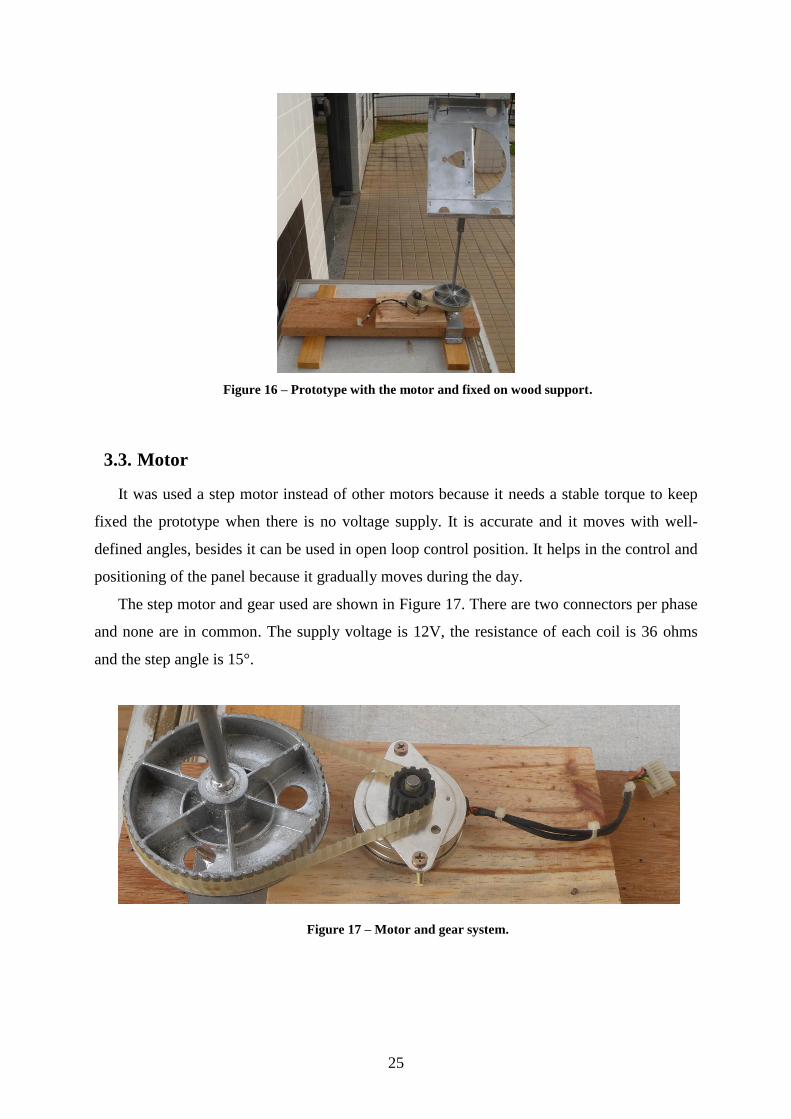
Figure 16 – Prototype with the motor and fixed on wood support.
3.3. Motor
It was used a step motor instead of other motors because it needs a stable torque to keep
fixed the prototype when there is no voltage supply. It is accurate and it moves with well-
defined angles, besides it can be used in open loop control position. It helps in the control and
positioning of the panel because it gradually moves during the day.
The step motor and gear used are shown in Figure 17. There are two connectors per phase
and none are in common. The supply voltage is 12V, the resistance of each coil is 36 ohms
and the step angle is 15°.
Figure 17 – Motor and gear system.
26
3.4. Drive and control strategy
A Microchip PIC 16F877 was used to control the solar tracker. A Integrated Circuit (IC)
ULN2004 was used to drain the current required for operation of the engine and a LCD
display shows the timing. The control system is based on time of day, in each hour the
prototype movement 15°.
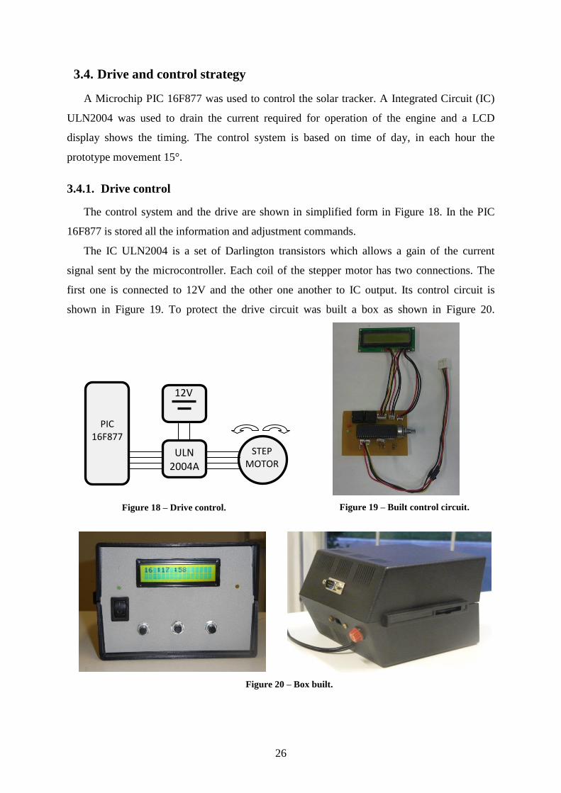
3.4.1. Drive control
The control system and the drive are shown in simplified form in Figure 18. In the PIC
16F877 is stored all the information and adjustment commands.
The IC ULN2004 is a set of Darlington transistors which allows a gain of the current
signal sent by the microcontroller. Each coil of the stepper motor has two connections. The
first one is connected to 12V and the other one another to IC output. Its control circuit is
shown in Figure 19. To protect the drive circuit was built a box as shown in Figure 20.
Figure 18 – Drive control.
Figure 19 – Built control circuit.
Figure 20 – Box built.
12V
PIC 16F877
ULN 2004A
STEP MOTOR

27
3.4.2. Control strategy
Once the system is started a welcome message request that the timer is set, Figure 21.
There is a button for set each minute and another for set each hour. When adjusted, the clock
operates normally and it is displayed on a 16x2 LCD display, Figure 22.
Figure 21 – Initial message.
Figure 22 – Timer.
After set the clock the algorithm makes the decision according to time-of-day. The initial
position is at 7 A.M. and the final position is at 6 P.M. Decisions are made as follows:
1- If the system is started between 7 A.M. and 6 P.M. the program calculates how much
the engine must act. If it is at 7 A.M., the structure keep in original position, otherwise
goes to the position corresponding to the time-of-day. Thereafter the panel begins to
follow the sun moving 15° every hour.
2- At 6:10 P.M. the microcontroller sends a command to the engine to return the panel to
the starting position.
3- If the clock is set to any range of different time from 7 A.M to 6 P.M the panel keeps
in the initial position until 8 A.M when it moves for the first time.
3.5. System data acquisition
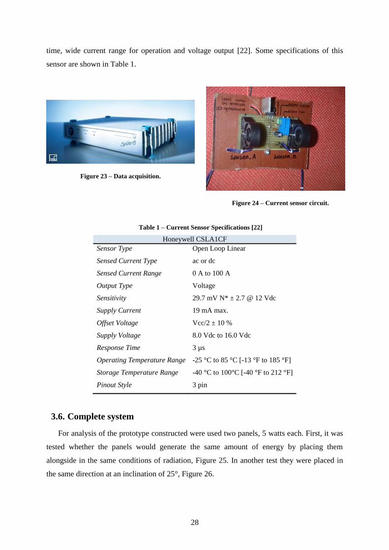
The Figure 23 show the acquisition system (SPIDER 8) used to allows measuring the
current and voltage in the experiment. The Spider 8 is an electronic measuring system for PCs
and is intended for measurement as voltage, power, pressure, acceleration and temperature.
The equipment has eight analog channels for data acquisition, a printer port, a PC/Master
connection, a socket with 25 pins (8 digital inputs and 8 digital inputs/outputs), a RS-232 port
and a connection to external power [21].
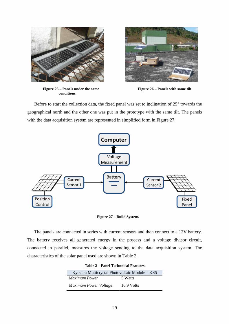
To measure the current generated by solar panel it was used a Honeywell CSLA1CF
current sensor, Figure 24. It is capable of measuring AC and DC current, it has a fast response
28
time, wide current range for operation and voltage output [22]. Some specifications of this
sensor are shown in Table 1.
Figure 23 – Data acquisition.
Figure 24 – Current sensor circuit.
Table 1 – Current Sensor Specifications [22]
Honeywell CSLA1CF
Sensor Type Open Loop Linear
Sensed Current Type ac or dc
Sensed Current Range 0 A to 100 A
Output Type Voltage
Sensitivity 29.7 mV N* ± 2.7 @ 12 Vdc
Supply Current 19 mA max.
Offset Voltage Vcc/2 ± 10 %
Supply Voltage 8.0 Vdc to 16.0 Vdc
Response Time 3 µs
Operating Temperature Range -25 °C to 85 °C [-13 °F to 185 °F]
Storage Temperature Range -40 °C to 100°C [-40 °F to 212 °F]
Pinout Style 3 pin
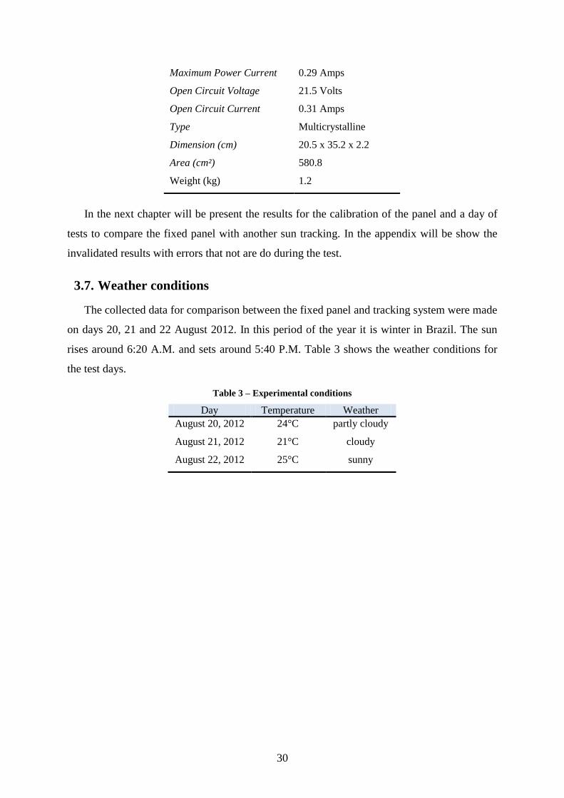
3.6. Complete system
For analysis of the prototype constructed were used two panels, 5 watts each. First, it was
tested whether the panels would generate the same amount of energy by placing them
alongside in the same conditions of radiation, Figure 25. In another test they were placed in
the same direction at an inclination of 25°, Figure 26.
29
Figure 25 – Panels under the same
conditions.
Figure 26 – Panels with same tilt.
Before to start the collection data, the fixed panel was set to inclination of 25° towards the
geographical north and the other one was put in the prototype with the same tilt. The panels
with the data acquisition system are represented in simplified form in Figure 27.
Figure 27 – Build System.
The panels are connected in series with current sensors and then connect to a 12V battery.
The battery receives all generated energy in the process and a voltage divisor circuit,
connected in parallel, measures the voltage sending to the data acquisition system. The
characteristics of the solar panel used are shown in Table 2.
Table 2 – Panel Technnical Features
Kyocera Multicrystal Photovoltaic Module – KS5
Maximum Power 5 Watts
Maximum Power Voltage 16.9 Volts
Battery
Voltage Measurement
Computer
Current Sensor 1
Current Sensor 2
Position Control
Fixed Panel
30
Maximum Power Current 0.29 Amps
Open Circuit Voltage 21.5 Volts
Open Circuit Current 0.31 Amps
Type Multicrystalline
Dimension (cm) 20.5 x 35.2 x 2.2
Area (cm²) 580.8
Weight (kg) 1.2
In the next chapter will be present the results for the calibration of the panel and a day of
tests to compare the fixed panel with another sun tracking. In the appendix will be show the
invalidated results with errors that not are do during the test.
3.7. Weather conditions
The collected data for comparison between the fixed panel and tracking system were made
on days 20, 21 and 22 August 2012. In this period of the year it is winter in Brazil. The sun
rises around 6:20 A.M. and sets around 5:40 P.M. Table 3 shows the weather conditions for
the test days.
Table 3 – Experimental conditions
Day Temperature Weather
August 20, 2012 24°C partly cloudy
August 21, 2012 21°C cloudy
August 22, 2012 25°C sunny
31
4. Results
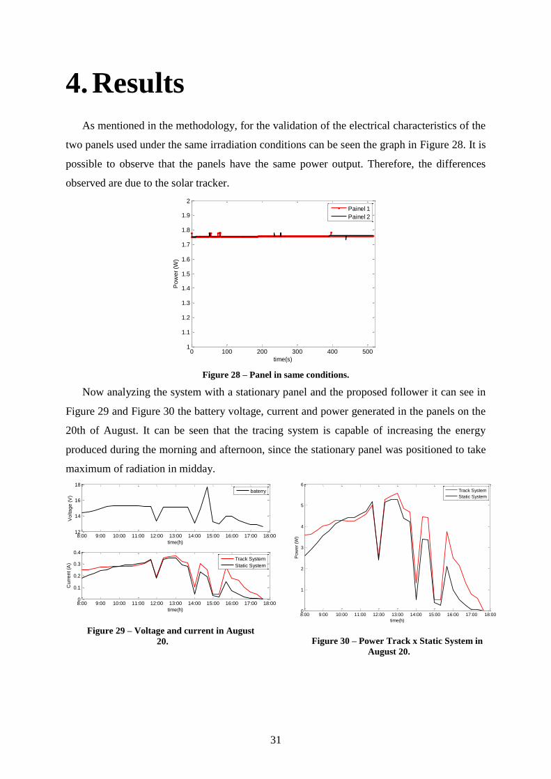
As mentioned in the methodology, for the validation of the electrical characteristics of the
two panels used under the same irradiation conditions can be seen the graph in Figure 28. It is
possible to observe that the panels have the same power output. Therefore, the differences
observed are due to the solar tracker.
Figure 28 – Panel in same conditions.
Now analyzing the system with a stationary panel and the proposed follower it can see in
Figure 29 and Figure 30 the battery voltage, current and power generated in the panels on the
20th of August. It can be seen that the tracing system is capable of increasing the energy
produced during the morning and afternoon, since the stationary panel was positioned to take
maximum of radiation in midday.
Figure 29 – Voltage and current in August
20.
Figure 30 – Power Track x Static System in
August 20.
0 100 200 300 400 5001
1.1
1.2
1.3
1.4
1.5
1.6
1.7
1.8
1.9
2
Po
we
r (W
)
time(s)
Painel 1
Painel 2
8:00 9:00 10:00 11:00 12:00 13:00 14:00 15:00 16:00 17:00 18:0012
14
16
18
Vo
lta
ge
(V
)
time(h)
baterry
8:00 9:00 10:00 11:00 12:00 13:00 14:00 15:00 16:00 17:00 18:000
0.1
0.2
0.3
0.4
Cu
rre
nt (A
)
time(h)
Track System
Static System
8:00 9:00 10:00 11:00 12:00 13:00 14:00 15:00 16:00 17:00 18:000
1
2
3
4
5
6
Po
we
r (W
)
time(h)
Track System
Static System
32
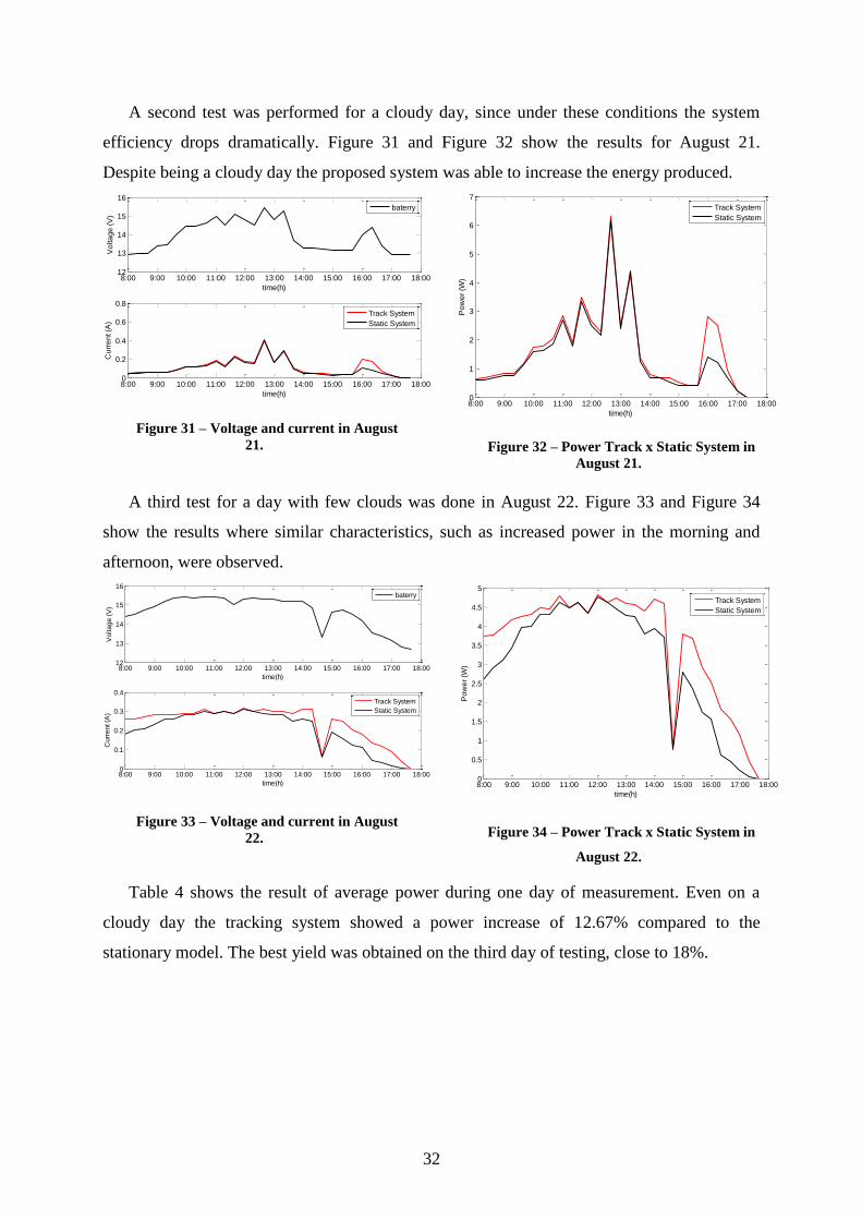
A second test was performed for a cloudy day, since under these conditions the system
efficiency drops dramatically. Figure 31 and Figure 32 show the results for August 21.
Despite being a cloudy day the proposed system was able to increase the energy produced.
Figure 31 – Voltage and current in August
21.
Figure 32 – Power Track x Static System in
August 21.
A third test for a day with few clouds was done in August 22. Figure 33 and Figure 34
show the results where similar characteristics, such as increased power in the morning and
afternoon, were observed.
Figure 33 – Voltage and current in August
22.
Figure 34 – Power Track x Static System in
August 22.
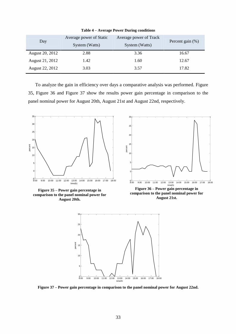
Table 4 shows the result of average power during one day of measurement. Even on a
cloudy day the tracking system showed a power increase of 12.67% compared to the
stationary model. The best yield was obtained on the third day of testing, close to 18%.
8:00 9:00 10:00 11:00 12:00 13:00 14:00 15:00 16:00 17:00 18:0012
13
14
15
16
Vo
lta
ge
(V
)
time(h)
baterry
8:00 9:00 10:00 11:00 12:00 13:00 14:00 15:00 16:00 17:00 18:000
0.2
0.4
0.6
0.8
Cu
rre
nt (A
)
time(h)
Track System
Static System
8:00 9:00 10:00 11:00 12:00 13:00 14:00 15:00 16:00 17:00 18:000
1
2
3
4
5
6
7
Po
we
r (W
)
time(h)
Track System
Static System
8:00 9:00 10:00 11:00 12:00 13:00 14:00 15:00 16:00 17:00 18:0012
13
14
15
16
Vo
lta
ge
(V
)
time(h)
baterry
8:00 9:00 10:00 11:00 12:00 13:00 14:00 15:00 16:00 17:00 18:000
0.1
0.2
0.3
0.4
Cu
rre
nt (A
)
time(h)
Track System
Static System
8:00 9:00 10:00 11:00 12:00 13:00 14:00 15:00 16:00 17:00 18:000
0.5
1
1.5
2
2.5
3
3.5
4
4.5
5
Po
we
r (W
)
time(h)
Track System
Static System
33
Table 4 – Average Power During conditions
Day Average power of Static
System (Watts)
Average power of Track
System (Watts) Percent gain (%)
August 20, 2012 2.88 3.36 16.67
August 21, 2012 1.42 1.60 12.67
August 22, 2012 3.03 3.57 17.82
To analyze the gain in efficiency over days a comparative analysis was performed. Figure
35, Figure 36 and Figure 37 show the results power gain percentage in comparison to the
panel nominal power for August 20th, August 21st and August 22nd, respectively.
Figure 35 – Power gain percentage in
comparison to the panel nominal power for
August 20th.
Figure 36 – Power gain percentage in
comparison to the panel nominal power for
August 21st.
Figure 37 – Power gain percentage in comparison to the panel nominal power for August 22nd.
8:00 9:00 10:00 11:00 12:00 13:00 14:00 15:00 16:00 17:00 18:00-5
0
5
10
15
20
25
30
35
perc
ent
time(h) 8:00 9:00 10:00 11:00 12:00 13:00 14:00 15:00 16:00 17:00 18:00-5
0
5
10
15
20
25
30
perc
ent
time(h)
8:00 9:00 10:00 11:00 12:00 13:00 14:00 15:00 16:00 17:00 18:000
5
10
15
20
25
30
perc
ent
time(h)

34
It was possible to see that largest increases in yield occur in the morning and afternoon,
when the stationary panel is no longer in its optimal position relative to the sun. The
construction’s price of the structure was approximately $20.00 and the drivers and
components $10.00.

35
5. Conclusion
This work shows the design, construction and validation of a one-axis Sun tracker. The
focus of the study was to develop a differentiated product of low cost, robust, able of tracking
the sun during the day and in the future could be easily earn different dimensions. These
characteristics provide conditions for it to be used in different types of environments and
applications.
The main difference of this work is the non-use of sensor. The use of this enhances the
equipment cost, in addition to increasing vulnerability due to some defect. Since the behavior
of the sun is well defined throughout the year, it is possible through preliminary studies define
the positions of the sun throughout the year, which is the technique used in this work. In turn,
the results showed that the model is effective even on a cloudy day of winter and the best
result was close to 18% on a sunny day.
More studies are needed mainly for large-scale construction.
36
Bibliography
[1] EUROPEAN PHOTOVOLTAIC INDUSTRY ASSOCIATION - EPIA. Global Market
Outlook for Photovoltaics Until 2015. 2012.
[2] AGÊNCIA NACIONAL DE ENERGIA ELÉTRICA - ANEEL. Atlas de Energia
Elétrica do Brasil. 3ª Edição. ed. Brasília, 2008.
[3] A. ELISEU BURDA, B. P. M. B. C. J. I. B. Evolution of Renewable Energy in Brazil.
International Conference on Clean Electrical Power (ICCEP), 2011. 316 - 319.
[4] CEPEL - CRESESB. Manual de Engenharia para Sistemas Fotovoltaicos. Rio de
Janeiro, 2004.
[5] SKVARENINA, T. L. The Power Electronics. Indiana: Purdue University, 2002.
[6] HOSSEIN MOUSAZADEH, A. K. A. J. H. M. K. A. A. S. A review of principle and
sun-tracking methods for maximizing solar systems output. Renewable and Sustainable
Energy Reviews, October 2009. 1800–1818.
[7] LAMBERTS, R. DESEMPENHO TÉRMICO DE EDIFICAÇÕES. 3ª. ed.
Florianópolis, 2005.
[8] MASTERS, G. M. Renewable and Efficient Electric Power Systems. 2004.
[9] DORADO, E. D. et al. Influence of the PV modules layout in the power losses of a PV
array with shadows. EPE, 2010.
[10] KARAZHANOV, S. Z. Temperature and doping level dependence of solar cell
performace including excitons. Solar Energy and Materials & Solar Cells, v. 63, n. 2,
p. 149-163, 2000.
[11] BRECL, K.; TOPIC, M. Self-shading losses of fixed free-standing PV arrays.
Renewable Energy, v. 36, n. 11, p. 3211 - 3216, 2011.
[12] PATEL, M. R. Wind and Solar Power Systems. 1999.
[13] MOORE'S Law for Solar - 30c watt in years to come, 2009. Disponivel em:
<http://www.dailykos.com/story/2009/12/15/807173/-Moore-s-Law-for-Solar-30c-watt-
in-years-to-come>. Acesso em: 2012.
[14] FARZIN SHAMA, G. H. R. A. A. S. R. A Novel Design and Experimental Study for a
Two-Axis Sun Tracker. Asia-Pacific Power and Energy Engineering Conference
(APPEEC), Wuhan, 2011.
[15] HAN DONG, W. Z. S. H. X. G. L. F. Research and Design on a Robust Sun-tracker.
International Conference on Sustainable Power Generation and Supply -
SUPERGEN, 2009. 1-6.
[16] J. BIONE, O. C. V. N. F. Comparison of the performance of PV water pumping systems
driven by fixed, tracking and V-trough generators. Solar Energy, n. 76, p. 703 - 711,
2004.
[17] TOMSON, T. Discrete two-positional tracking of solar collectors. Renewable Energy,
2008. 400 - 405.
[18] I.M. MICHAELIDES, S. A. K. I. C. G. R. A. H. Comparison of performance and cost
effectiveness of solar water heaters at different collector tracking modes in Cyprus and
Greece. Energy Conversion & Management, 1999. 1287 - 1303.
[19] CHEN, X. et al. Experimental Study of the Uniaxial Automatic Solar Tracking Device
Towards Sun Comparison with Fixed Bracket. Asia-Pacific Power and Energy

37
Engineering Conference (APPEEC), Wuhan, April 2011. 1-4.
[20] PONNIRAN, A.; HASHIM, A.; MUNIR, H. A. A design of single axis sun tracking
system. 5th International Power Engineering and Optimization Conference
(PEOCO), Shah Alam, June 2011. 107-110.
[21] HBM, H. B. M.-. Eletrônica de medição para PC, Spider8 - Manual de Operação.
[22] HONEYWELL. CSLA1CF - Datasheet. Disponivel em:
<http://www.compel.ru/images/catalog/334/CSLA1CF.htm>.
38
Appendix A
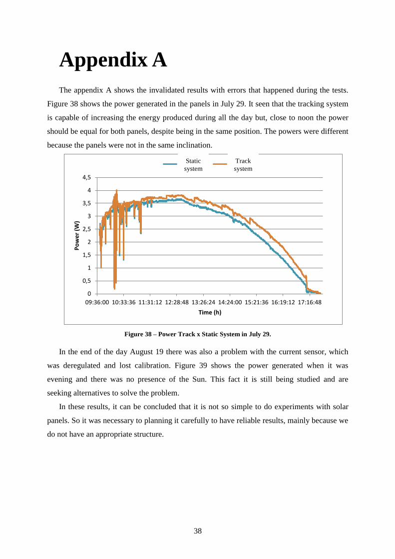
The appendix A shows the invalidated results with errors that happened during the tests.
Figure 38 shows the power generated in the panels in July 29. It seen that the tracking system
is capable of increasing the energy produced during all the day but, close to noon the power
should be equal for both panels, despite being in the same position. The powers were different
because the panels were not in the same inclination.
Figure 38 – Power Track x Static System in July 29.
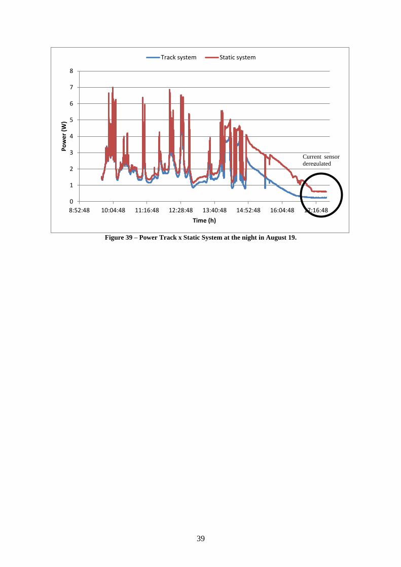
In the end of the day August 19 there was also a problem with the current sensor, which
was deregulated and lost calibration. Figure 39 shows the power generated when it was
evening and there was no presence of the Sun. This fact it is still being studied and are
seeking alternatives to solve the problem.
In these results, it can be concluded that it is not so simple to do experiments with solar
panels. So it was necessary to planning it carefully to have reliable results, mainly because we
do not have an appropriate structure.
0
0,5
1
1,5
2
2,5
3
3,5
4
4,5
09:36:00 10:33:36 11:31:12 12:28:48 13:26:24 14:24:00 15:21:36 16:19:12 17:16:48
Po
we
r (W
)
Time (h)
Power Not PowerTrack
system
Static
system
39
Figure 39 – Power Track x Static System at the night in August 19.
0
1
2
3
4
5
6
7
8
8:52:48 10:04:48 11:16:48 12:28:48 13:40:48 14:52:48 16:04:48 17:16:48
Po
we
r (W
)
Time (h)
Track system Static system
Current sensor
deregulated

40
Appendix B
In this appendix is shown the paper, “A Low-Cost Prototype for Sun Tracking”, based on
this work that was published in 10th IEEE/IAS International Conference on Industry
Applications, 2012, Fortaleza, Brazil.
1
Resumo Expandido
Desenvolvimento de um Seguidor Solar
Gabriel Akira Gomes Ribeiro, Heverton Augusto Pereira
1. Introdução
O aumento na demanda energética, juntamente
com o apelo para o uso de fontes menos poluentes
leva os principais centros de pesquisa a buscarem
novas formas de produção de energia. Uma delas é a
tecnologia de painéis fotovoltaicos (PV), que nos
últimos anos, devido ao crescimento robusto e
contínuo, mostrou o potencial para se tornar uma
fonte importante de geração de energia para o
mundo. PV é agora, depois de hidrelétricas e energia
eólica, a energia renovável mais importante e a
terceira em termos de capacidade instalada a nível
mundial [1].
Atualmente, existem vários projetos utilizando
energia solar no Brasil, principalmente para o
atendimento de comunidades isoladas das redes de
energia e desenvolvimento regional. Os principais
tipos de projetos são: o bombeamento de água para
abastecimento doméstico, irrigação e piscicultura;
Iluminação, sistemas de uso coletivo, tais como
eletrificação de escolas, centros de saúde e centros
comunitários; instalação em casa [2].
A energia solar chega à Terra nas formas
térmica e luminosa. No entanto, não atinge de
maneira uniforme toda a crosta terrestre. Ela
depende da latitude, da época e das condições
climáticas, como nebulosidade e umidade relativa.
As regiões que recebem mais radiação solar
estão localizadas entre os Trópicos: Câncer no
hemisfério norte e Capricórnio no hemisfério sul. A
radiação solar que atinge a atmosfera terrestre é
dividida em direta e difusa. A radiação direta é a
parte que vai diretamente para a terra. A radiação
difusa é a parte que sofre um espalhamento por
nuvens e partículas na atmosfera. Um céu nublado
pode ter uma maior proporção de radiação difusa,
enquanto o céu claro, sem nuvens, apresenta maior
de radiação direta [3].
Em muitas situações é útil saber como estimar
no céu, em determinada hora e dia do ano, onde o
sol vai estar. No caso da energia solar, a fim de
capturar maior insolação, é possível utilizar o
conhecimento sobre ângulos solares para escolher o
melhor ângulo de inclinação para posicionar os
módulos solares, pois quanto mais se aproveitar a
radiação solar melhor, já que os painéis solares mais
avançados convertem de 10% a 15% de radiação em
energia.
A localização do sol durante do dia pode ser
descrita em termos do ângulo de altitude (β) e o
ângulo de azimute (ϕs), como é mostrado na Figura
1.
O ângulo β é definido como o ângulo vertical
entre os raios solares e a projeção dos mesmos no
plano horizontal.
O ângulo ϕs é o ângulo horizontal medido a
partir do sul (no hemisfério norte) para a projeção
horizontal dos raios do sol [4].
Figura 1: Posição do Sol descrita pelo ângulo de
altitude (β) e o ângulo de azimute (ϕs).
Mais energia é recolhida no final do dia se o
módulo PV é instalado sobre um rastreador solar que
funcionará como um girassol. O rastreador
2
introduzido pela primeira vez por Finster, em 1962,
era completamente mecânico. Um ano mais tarde,
Saavedra apresentou um mecanismo com um
controle eletrônico automático utilizando um
piranômetro, instrumento usado para medir radiação
[4]. Um projeto de monitoramento do sol pode
aumentar a energia gerada em até 40 por cento ao
longo do ano em relação a outro com painel fixo. O
seguidor solar pode ser de um ou dois eixos [5].
O seguidor solar de um eixo segue o sol de leste
a oeste durante o dia, acompanhando as mudanças
no ângulo de azimute [5]. A Figura 2 mostra
exemplos deste tipo de seguidor.
Figura 2: Seguidor solar de um eixo.
Um seguidor solar de dois eixos localiza o sol
de leste a oeste durante o dia, e de norte a sul
durante as estações do ano, na Figura 3 são
apresentados exemplos de seguidor solar de dois
eixos. O rastreamento de duplo eixo é feita por dois
motores atuação linear [5].
Figura 3: Seguidor solar de dois eixos.
Em [6] comparou-se resultados de um sistema
de bombeamento de água, em Recife (PE-Brasil),
alimentado por painel fixo, painel com rastreamento
e um terceiro utilizando espelhos para concentrar os
raios solares e rastreamento. O modelo PV gerador
com concentrador é constituído por quatro pares de
espelhos e quatro painéis, os modelos com seguidor
fazem o rastreamento ao longo do eixo Norte-Sul,
inclinados em um ângulo de 20° em direção ao
norte. A vantagem em termos de radiação solar, para
painéis com rastreamento é igual a 1,23 e para o
seguidor com coletores de concentração, é igual a
1,74. Estes valores para o volume de água são 1,41 e
2,49, respectivamente.
Tomson comparou diariamente o desempenho
de um sistemas PV com rastreamento de dois eixos.
As posições simétricas e assimétricas em torno do
eixo norte-sul, correspondentes às posições de sol de
manhã e à tarde, foram analisadas. De acordo com
isto, foram avaliados os efeitos de diferentes ângulos
de inclinação e azimute iniciais, durante o dia e em
diferentes estações. Os resultados mostram que o
aumento de energia foi de 10-20% sobre o
rendimento de um painel fixo com ângulo de
inclinação ideal [7].
Michaelides estudou o desempenho térmico e o
custo efetivo de aquecedores de água solares com
diferentes modos de rastreamento solar sob o clima e
as condições socioeconômicas de Nicósia (Chipre) e
Atenas (Grécia). Ele fez comparações de quatro
diferentes maneiras usando o programa de simulação
TRNSYS: um sistema fixo inclinado 40°, um
segundo utilizando rastreamento com o eixo vertical,
o terceiro com variação do ângulo de azimute e
outro com modo de rastreamento sazonal onde a
inclinação do coletor é trocada duas vezes por ano.
Os resultados de simulação mostraram que o melhor
desempenho térmico foi obtido com o controle do
eixo vertical. Em Nicosia, a radiação solar anual
com este modo foi de 87,6% comparado com 81,6%
com o modo de sazonal e para 79,7% com o modo
fixo, enquanto que os valores correspondentes para a
Athens foi 81,4%, 76,2% e 74,4%, respectivamente.
3
Do ponto de vista econômico, o modo de captação
com painel fixo para ser o mais rentável [8].
Farzin mostrou em [9] um pequeno rastreador
solar de dois eixos com três algoritmos de controle
para motores de passo. O primeiro algoritmo propõe
mover a estrutura com pequenos passos em
coordenadas circulares e encontrar o ponto com a
melhor tensão gerada. O segundo algoritmo,
encontra a inclinação da melhor tensão e o terceiro é
semelhante ao segundo, mas é usado para encontrar
alguns pontos distintos em épocas diferentes.
Chen compara a irradiação solar para um painel
fixo e um seguidor solar de um eixo com controle
automático. O sistema foi produzido pela Kunming
green electrical science and technology Ltd, seu
nome é Rack Sun. Foram feitas três dias de teste
com boas condições climáticas para mostrar que o
sistema proposto pode aumentar a quantidade de
eletricidade gerada em 25 ~ 28% [10].
Ponniran projetou um seguidor solar de um eixo
para uso residencial e comparou com painel solar
parado. No protótipo foi utilizado um
microcontrolador PIC16F877A e o controle é
baseado em sinais de dois Resistor Dependente de
Luz diferente (LDR). Os resultados mostram que o
sistema permite um ganho considerável de energia
durante o dia, principalmente no período da manhã
[11].
2. Metodologia
2.1. Estudo do movimento aparente do Sol
O objetivo principal foi interpretar as variações
do ângulo de azimute e altitude durante o dia. Para
isto, foi utilizado o software Satellite Antenna
Alignment que fornece o valor de altitude e azimute
cada minuto. Com os dados foram construídos
gráficos para cada mês utilizando a informação para
a cidade de Viçosa-MG, latitude -20° 45'. A Figura 4
mostra o gráfico construído e permite uma visão
mais clara de como ocorre a variação na posição do
sol durante o dia em diferentes épocas do ano.
O ângulo de azimute tem maior variação entre
11:00-13:00 horas, principalmente durante o verão.
Os meses com maior incidência de raios solares são
Novembro, Dezembro e Janeiro. No entanto, durante
este período, há uma grande concentração de
nuvens, resultando numa componente de radiação
difusa maior do que a radiação direta.
2.2. Construção do protótipo
A ideia inicial foi construir um protótipo
simples, resistente e utilizando poucos materiais.
Assim, para um primeiro projeto, optou-se por
construir um seguidor solar de um eixo com
regulagem manual para inclinação.
A base foi feita de ferro, porque é mais pesado e
ajuda na sustentação. Em seguida foi adicionado um
rolamento para reduzir a força motriz necessária
para mover a estrutura. Logo acima do rolamento há
uma engrenagem, semelhante ao encontrado em uma
máquina de lavar roupa, que está em contato com o
motor por meio de outra menor ligada a uma correia,
sendo a relação de engrenagem igual a 24:1. O
restante da estrutura é feita de alumínio, material
leve e resistente, capaz de suportar o painel solar e
sofrer menos danos ao longo do tempo.
4
Figura 4: Variação de azimute e altura solar durante o ano para a cidade de Viçosa-MG.
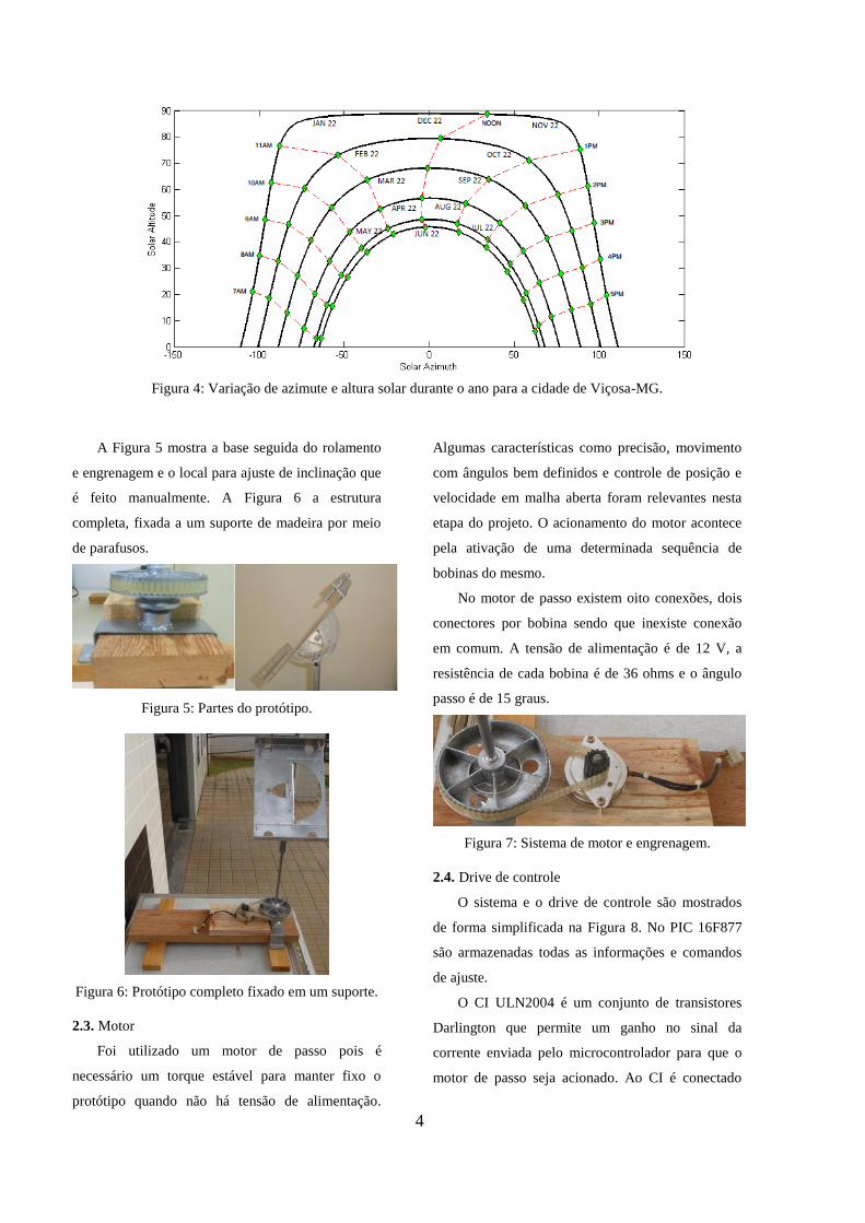
A Figura 5 mostra a base seguida do rolamento
e engrenagem e o local para ajuste de inclinação que
é feito manualmente. A Figura 6 a estrutura
completa, fixada a um suporte de madeira por meio
de parafusos.
Figura 5: Partes do protótipo.
Figura 6: Protótipo completo fixado em um suporte.
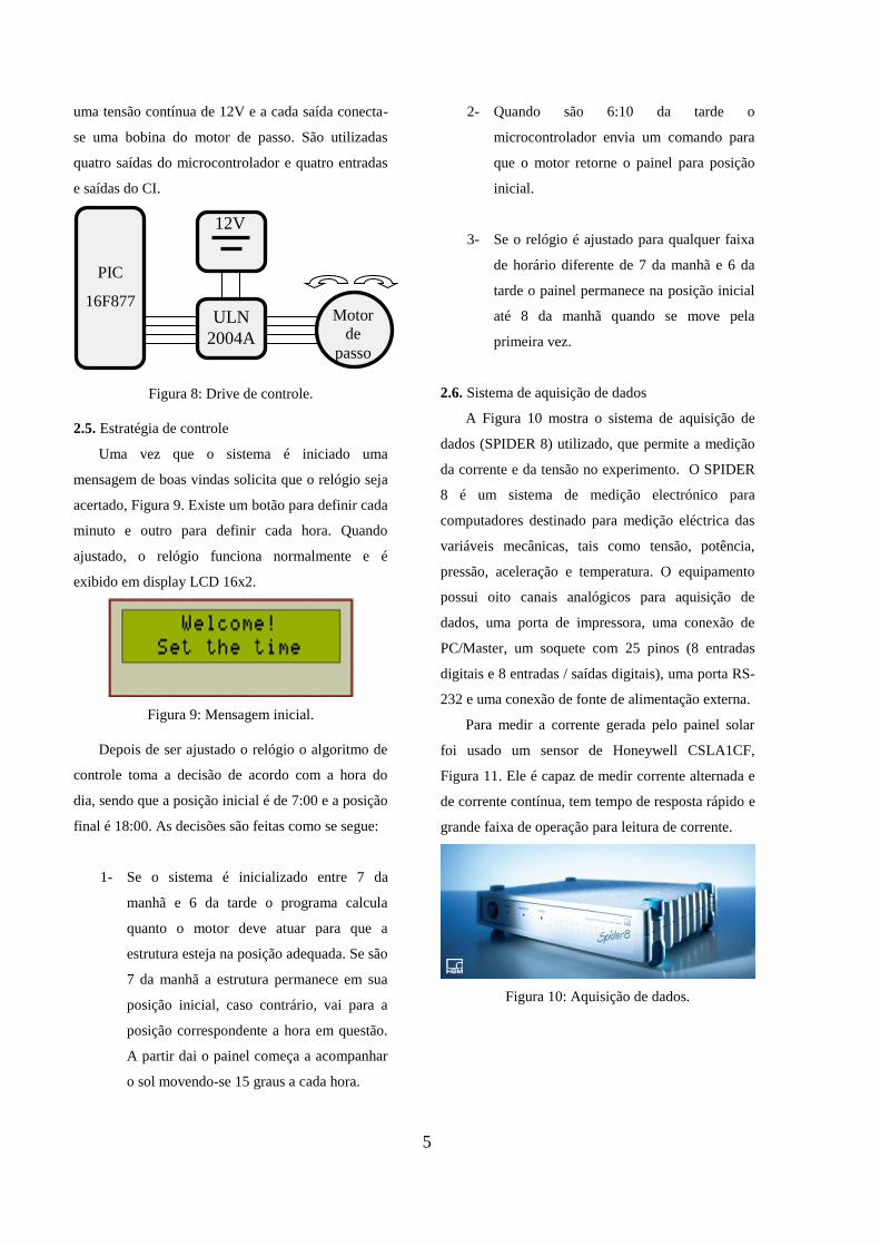
2.3. Motor
Foi utilizado um motor de passo pois é
necessário um torque estável para manter fixo o
protótipo quando não há tensão de alimentação.
Algumas características como precisão, movimento
com ângulos bem definidos e controle de posição e
velocidade em malha aberta foram relevantes nesta
etapa do projeto. O acionamento do motor acontece
pela ativação de uma determinada sequência de
bobinas do mesmo.
No motor de passo existem oito conexões, dois
conectores por bobina sendo que inexiste conexão
em comum. A tensão de alimentação é de 12 V, a
resistência de cada bobina é de 36 ohms e o ângulo
passo é de 15 graus.
Figura 7: Sistema de motor e engrenagem.
2.4. Drive de controle
O sistema e o drive de controle são mostrados
de forma simplificada na Figura 8. No PIC 16F877
são armazenadas todas as informações e comandos
de ajuste.
O CI ULN2004 é um conjunto de transistores
Darlington que permite um ganho no sinal da
corrente enviada pelo microcontrolador para que o
motor de passo seja acionado. Ao CI é conectado
5
uma tensão contínua de 12V e a cada saída conecta-
se uma bobina do motor de passo. São utilizadas
quatro saídas do microcontrolador e quatro entradas
e saídas do CI.
Figura 8: Drive de controle.
2.5. Estratégia de controle
Uma vez que o sistema é iniciado uma
mensagem de boas vindas solicita que o relógio seja
acertado, Figura 9. Existe um botão para definir cada
minuto e outro para definir cada hora. Quando
ajustado, o relógio funciona normalmente e é
exibido em display LCD 16x2.
Figura 9: Mensagem inicial.
Depois de ser ajustado o relógio o algoritmo de
controle toma a decisão de acordo com a hora do
dia, sendo que a posição inicial é de 7:00 e a posição
final é 18:00. As decisões são feitas como se segue:
1- Se o sistema é inicializado entre 7 da
manhã e 6 da tarde o programa calcula
quanto o motor deve atuar para que a
estrutura esteja na posição adequada. Se são
7 da manhã a estrutura permanece em sua
posição inicial, caso contrário, vai para a
posição correspondente a hora em questão.
A partir dai o painel começa a acompanhar
o sol movendo-se 15 graus a cada hora.
2- Quando são 6:10 da tarde o
microcontrolador envia um comando para
que o motor retorne o painel para posição
inicial.
3- Se o relógio é ajustado para qualquer faixa
de horário diferente de 7 da manhã e 6 da
tarde o painel permanece na posição inicial
até 8 da manhã quando se move pela
primeira vez.
2.6. Sistema de aquisição de dados
A Figura 10 mostra o sistema de aquisição de
dados (SPIDER 8) utilizado, que permite a medição
da corrente e da tensão no experimento. O SPIDER
8 é um sistema de medição electrónico para
computadores destinado para medição eléctrica das
variáveis mecânicas, tais como tensão, potência,
pressão, aceleração e temperatura. O equipamento
possui oito canais analógicos para aquisição de
dados, uma porta de impressora, uma conexão de
PC/Master, um soquete com 25 pinos (8 entradas
digitais e 8 entradas / saídas digitais), uma porta RS-
232 e uma conexão de fonte de alimentação externa.
Para medir a corrente gerada pelo painel solar
foi usado um sensor de Honeywell CSLA1CF,
Figura 11. Ele é capaz de medir corrente alternada e
de corrente contínua, tem tempo de resposta rápido e
grande faixa de operação para leitura de corrente.
Figura 10: Aquisição de dados.
12V
PIC
16F877 ULN
2004A
Motor
de
passo
6
Figura 11: Circuito do sensor de corrente.
2.7. Sistema completo
Para a análise do protótipo construído foram
usados dois painéis, cada um de cinco watts.
Primeiro, testou se os painéis geravam a mesma
quantidade de energia colocando-os em paralelo
sobre mesmas condições de radiação. Num outro
teste, estas foram colocadas na mesma direção com
uma inclinação de 25°.
Antes de iniciar a coleta de dados, o painel fixo
foi colocado com uma inclinação de 25° para o norte
geográfico e o outro sobre o protótipo com a mesma
inclinação. Os painéis com o sistema de aquisição de
dados estão representados de forma simplificada na
Figura 12.
Os painéis são ligados em série com sensores de
corrente que, em seguida, conectam-se a uma bateria
de 12V. A bateria recebe toda a energia gerada no
processo e de um circuito divisor de tensão, ligados
em paralelo, é medida a tensão e feita a leitura pelo
sistema de aquisição de dados. As características dos
painéis utilizados são mostradas na Tabela 1.
Figura 12: Sistema completo para medições.
Tabela 1 – Características do painel solar
Painel fotovoltaico Kyocera – KS5
Potência máxima 5 Watts
Tensão de máxima potência 16.9 Volts
Corrente de máxima potência 0.29 Amps
Tensão de circuito aberto 21.5 Volts
Corrente de circuito aberto 0.31 Amps
Tipo Multicristalino
Dimensão (cm) 20.5 x 35.2 x 2.2
Área (cm²) 580.8
Peso (kg) 1.2
2.8. Condições climáticas
As medições para a comparação entre o painel
fixo e sistema de rastreamento foram feitas nos dias
20, 21 e 22 agosto de 2012. Neste período do ano é
inverno no Brasil, na cidade de Viçosa o sol nasce
em torno de 6:20 da manhã e se põe perto de 05:40
da tarde. A Tabela 2 mostra as condições do tempo
para os dias de teste.
Tabela 2 – Condições climáticas
Dia Temperatura Tempo
20/08/2012 24°C Parcialmente nublado
21/08/2012 21°C Nublado
22/08/2012 25°C Ensolarado
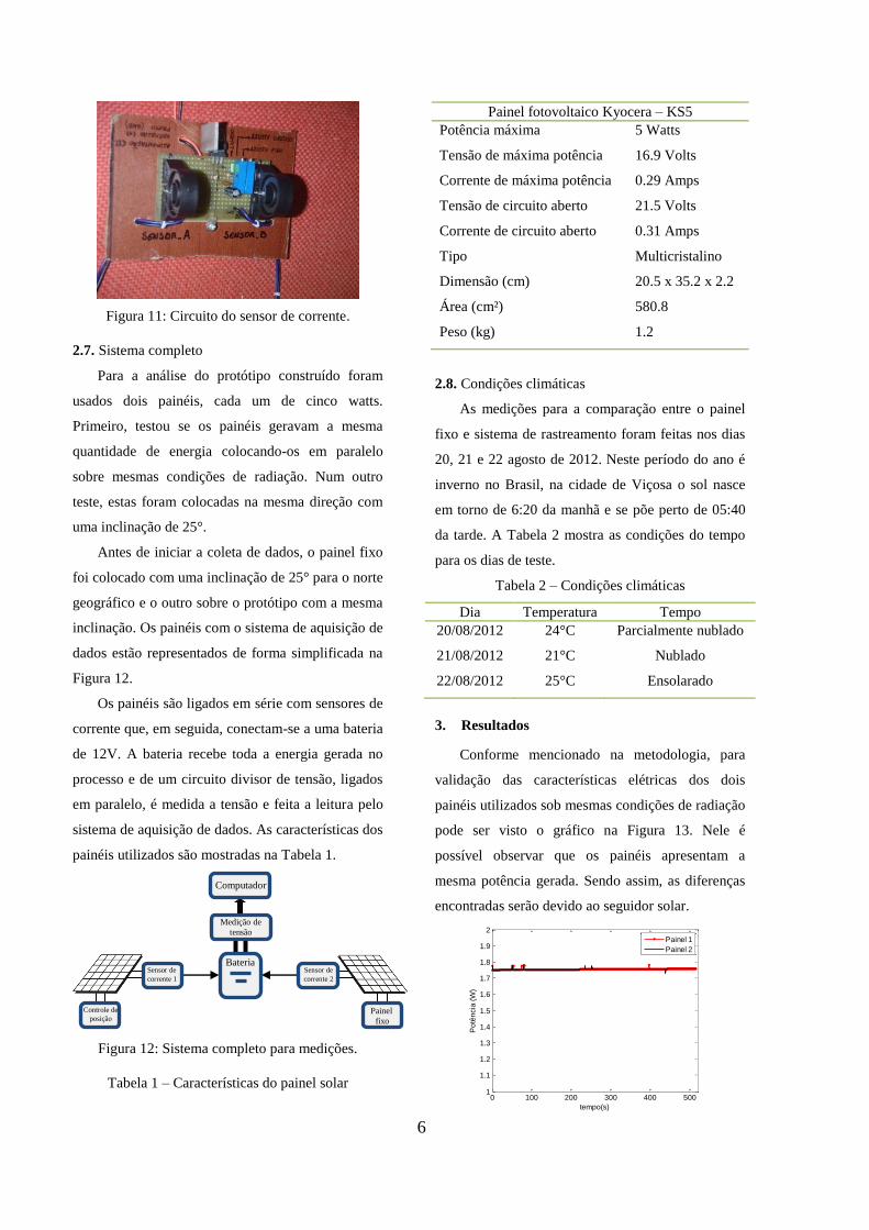
3. Resultados
Conforme mencionado na metodologia, para
validação das características elétricas dos dois
painéis utilizados sob mesmas condições de radiação
pode ser visto o gráfico na Figura 13. Nele é
possível observar que os painéis apresentam a
mesma potência gerada. Sendo assim, as diferenças
encontradas serão devido ao seguidor solar.
0 100 200 300 400 500
1
1.1
1.2
1.3
1.4
1.5
1.6
1.7
1.8
1.9
2
Po
tên
cia
(W
)
tempo(s)
Painel 1
Painel 2
Bateria
Medição de
tensão
Computador
Sensor de
corrente 1 Sensor de
corrente 2
Controle de
posição Painel
fixo

7
Figura 13: Potência dos painéis em mesmas
condições.
Agora analisando o sistema com um painel
estacionário e o seguidor proposto é possível
observar na Figura 14 a potência gerada no dia 20 de
Agosto. Pode ser visto que o sistema de rastreio é
capaz de aumentar a energia produzida durante o
período da manhã e da tarde, já que o painel
estacionário foi posicionado para ter máximo
aproveitamento ao meio dia.
Figura 14: Potência painel com seguidor x painel
fixo em 20 de Agosto.
Um segundo teste foi realizado para um dia
nublado, já que nessas condições a eficiência do
sistema cai drasticamente. A Figura 15 mostra o
resultado para o dia 21 de agosto. Apesar de ser um
dia nublado o sistema proposto foi capaz de
aumentar a energia produzida.
Figura 15: Potência painel com seguidor x painel
fixo em 21 de Agosto.
Um terceiro teste para um dia com poucas
nuvens foi realizado em 22 de Agosto. A Figura 16
mostra o resultado onde características semelhantes,
como aumento de potência de manha e a tarde,
foram observadas.
Figura 16: Potência painel com seguidor x painel
fixo em 22 de Agosto.
A Tabela 3 mostra o resultado da potência
média durante um dia de medição. Mesmo em um
dia nublado o sistema de rastreamento mostrou um
aumento de potência de 12,67% em relação ao
modelo estacionário. O melhor rendimento foi
obtido no terceiro dia de testes, próximo a 18%.
Tabela 3 – Potência média durante o dia
Dia
Potência média
– painel fixo
(Watts)
Potência média
– painel com
rastreamento
(Watts)
Ganho
percentual (%)
20/08/2012 2,88 3,36 16,67
21/08/2012 1,42 1,60 12,67
22/08/2012 3,03 3,57 17,82
Para analisar o ganho em eficiência ao longo do
dia, as Figura 17, Figura 18 e Figura 19 mostram a
percentagem do ganho de potência do sistema com
rastreamento solar em relação a potência nominal do
painel para os dias de teste.
8:00 9:00 10:00 11:00 12:00 13:00 14:00 15:00 16:00 17:00 18:000
1
2
3
4
5
6
Po
tên
cia
(W
)
tempo(h)
Seguidor solar
Painel fixo
8:00 9:00 10:00 11:00 12:00 13:00 14:00 15:00 16:00 17:00 18:000
1
2
3
4
5
6
7
Po
tên
cia
(W
)
tempo(h)
Seguidor solar
Painel fixo
8:00 9:00 10:00 11:00 12:00 13:00 14:00 15:00 16:00 17:00 18:000
0.5
1
1.5
2
2.5
3
3.5
4
4.5
5
Po
tên
cia
(W
)
tempo(h)
Seguidor solar
Painel fixo

8
Figura 17: Ganho de potência em função da potência
máxima do painel para 20 de Agosto.
Figura 18: Ganho de potência em função da potência
máxima do painel para 21 de Agosto.
Figura 19: Ganho de potência em função da potência
máxima do painel para 22 de Agosto.
Como foi possível perceber os maiores
aumentos de rendimento ocorrem na parte da manhã
e da tarde, quando o painel estacionário não está
mais em sua posição ótima em relação ao sol.
O preço de construção da estrutura foi de
aproximadamente R$40,00 e os drivers e
componentes R$20,00.
4. Conclusion
Este trabalho mostra o projeto, construção e
validação de um seguidor solar de um eixo. O foco
do trabalho foi desenvolver um produto diferenciado
de baixo custo, robusto, capaz de rastrear o sol
durante o dia e que posteriormente pudesse
facilmente ganhar diferentes dimensões. Essas
características dão condições para que o mesmo seja
utilizados em diferentes tipos de ambientes e
aplicações.
A principal diferença deste trabalho é a não
utilização do uso do sensor, pois o mesmo
aumentaria a vulnerabilidade devido a algum
defeito. Como o comportamento do sol é bem
definido ao longo do ano, é possível através de
estudos preliminares definir as posições do sol ao
longo do ano, sendo esta a técnica utilizada neste
trabalho. Por sua vez, os resultados mostraram que o
modelo apresenta eficácia mesmo em um dia
nublado de inverno e o melhor resultado ficou
próximo a 18% num dia ensolarado.
Mais estudos precisam ser realizados
principalmente para a construção em larga escala.
8:00 9:00 10:00 11:00 12:00 13:00 14:00 15:00 16:00 17:00 18:00-5
0
5
10
15
20
25
30
35
Ganho p
erc
entu
al
tempo(h)
8:00 9:00 10:00 11:00 12:00 13:00 14:00 15:00 16:00 17:00 18:00-5
0
5
10
15
20
25
30
Ganho p
erc
entu
al
tempo(h)
8:00 9:00 10:00 11:00 12:00 13:00 14:00 15:00 16:00 17:00 18:000
5
10
15
20
25
30
Ganho p
erc
entu
al
tempo(h)