development of an energy management model for chalmers...

Development of an energy managementmodel for Chalmers’ microgrid:Application for cost-benefit analysis of battery energy stor-age

Master’s thesis in Electric Power Engineering

MARTIN GÖRANSSONNIKLAS LARSSON

Department of Energy and EnvironmentCHALMERS UNIVERSITY OF TECHNOLOGYGothenburg, Sweden 2016

Master’s thesis 2016

Development of an energy management model forChalmers’ microgrid: Application for cost-benefit

analysis of battery energy storage

MARTIN GÖRANSSONNIKLAS LARSSON

Department of Energy and EnvironmentDivision of Electric Power Engineering

Chalmers University of TechnologyGothenburg, Sweden 2016

Development of an energy management model for Chalmers’ microgridApplication for cost-benefit analysis of battery energy storageMartin GöranssonNiklas Larsson

© Martin GöranssonNiklas Larsson, 2016.

Supervisor and Examiner: Anh Tuan Le, Division of Electric Power Engineering

Department of Energy & EnvironmentDivision of Electric Power EngineeringChalmers University of TechnologySE-412 96 GothenburgSwedenTelephone +46 31 772 1000

iv

Development of an energy management model for Chalmers’ microgrid: Applicationfor cost-benefit analysis of battery energy storageNiklas LarssonMartin GöranssonDepartment of Energy & EnvironmentChalmers University of Technology

AbstractA microgrid is a portion of a larger grid which can be operated independently, thus itis seen as a single entity from the main grid which can be operated in grid connectedor island mode. The microgrid consists of distributed energy resources (DER), en-ergy storage system (ESS) and loads which can be controllable. This thesis is apre-study regarding Chalmers’ grid as a microgrid. The aim of this thesis is toevaluate the technical and economical performance of Chalmers’ microgrid. In thisthesis, a database containing grid data and load profiles for the Chalmers’ grid wasestablished. This database was used as input in the developed energy managementmodel (EMM) for the microgrid, which is a planning model used to schedule andoptimize own generation, flexible loads and energy storage within the microgrid. Amicrogrid simulation platform (MSP) was developed containing the EMM in GAMSand data handling in MATLAB enabling simulations with varying input parameterssuch as ESS capacity and its location.

The MSP is used for benefit-cost analysis of different ESS sizes and locations, andfinally for case studies regarding increased amounts of renewable energy (solar PV),island mode operation and vehicle to grid technology (V2G). Results from the anal-ysis show that the total annual cost of electricity can be reduced by 8.43% byincluding 6 MWh of Li-ion battery storage and increasing the amount of local solarenergy to 3 MWp, while also enabling the grid to be operated in island mode for1 hour periods. With today’s battery prices and expected lifetime, investing in ahigher amount of solar PVs and a smaller ESS yields the best investment. The casestudies show that running the microgrid in island operation is possible, however todo so for a long time requires a large size of ESS. By running part of Chalmers’ gridas a microgrid, thus having a higher generation to load ratio, the ESS size couldbe decreased. With increases in renewable energy capacity at Chalmers, the size ofbatteries to accomplish island-mode operation is reduced. The V2G technology en-ables the batteries of the vehicles to act as a distributed ESS. The results show thatthe benefits gained by including electric vehicles are less than the benefits gainedby stationary battery storage. This is due to the vehicles being present within thegrid during daytime, thus the batteries cannot be charged during the night whenelectricity prices are lower. There are economical benefits to be gained from oper-ating Chalmers’ grid as a microgrid, however, the investment cost in battery energystorage today is high compared to the benefits gained. Other benefits gained bymicrogrid operation include enhanced reliability and increased local control.Keywords: Optimal power flow (OPF), Microgrid, Campus, Energy storage system(ESS), Cost-benefit analysis

v

AcknowledgementsFirstly, we would like tot thank our supervisor Anh Tuan Le for all his help andsupport. We would also like to thank Richard Block, Per Löveryd and their col-leagues at Akademiska Hus for helping out with measurements and grid data forChalmers. Finally we would like to thank David Steen for his help and expertiseregarding GAMS modeling.

Niklas Larsson & Martin Göransson, Gothenburg, December 2016

vii

Contents

List of Figures xiii

List of Tables xv

List of Abbreviations xvii

List of Symbols xix

1 Introduction 11.1 Background and Motivations . . . . . . . . . . . . . . . . . . . . . . . 11.2 Objectives . . . . . . . . . . . . . . . . . . . . . . . . . . . . . . . . . 21.3 Specific tasks . . . . . . . . . . . . . . . . . . . . . . . . . . . . . . . 21.4 Scope . . . . . . . . . . . . . . . . . . . . . . . . . . . . . . . . . . . 31.5 Thesis outline . . . . . . . . . . . . . . . . . . . . . . . . . . . . . . . 3

2 Technical background 52.1 The microgrid concept . . . . . . . . . . . . . . . . . . . . . . . . . . 52.2 Key components of a typical microgrid . . . . . . . . . . . . . . . . . 6

2.2.1 Electrical distribution grid . . . . . . . . . . . . . . . . . . . . 62.2.2 Distributed power generation . . . . . . . . . . . . . . . . . . 7

2.2.2.1 Combined heat and power . . . . . . . . . . . . . . . 72.2.2.2 Solar Photovoltaics generation . . . . . . . . . . . . . 72.2.2.3 Wind power . . . . . . . . . . . . . . . . . . . . . . . 8

2.2.3 Energy storage . . . . . . . . . . . . . . . . . . . . . . . . . . 82.2.3.1 Batteries . . . . . . . . . . . . . . . . . . . . . . . . 92.2.3.2 Vehicle to grid (V2G) . . . . . . . . . . . . . . . . . 92.2.3.3 Flywheel . . . . . . . . . . . . . . . . . . . . . . . . 92.2.3.4 Supercapacitors . . . . . . . . . . . . . . . . . . . . . 10

2.3 Features of microgrids . . . . . . . . . . . . . . . . . . . . . . . . . . 102.3.1 Demand response . . . . . . . . . . . . . . . . . . . . . . . . . 102.3.2 Energy management system in microgrids . . . . . . . . . . . 11

2.4 Previous Work . . . . . . . . . . . . . . . . . . . . . . . . . . . . . . 112.4.1 Sizing of Energy Storage Systems . . . . . . . . . . . . . . . . 112.4.2 Experimental Microgrids . . . . . . . . . . . . . . . . . . . . . 12

2.4.2.1 CERTS testbed US . . . . . . . . . . . . . . . . . . . 122.4.2.2 University of Texas at Arlington microgrid testbed . 12

ix

Contents

2.4.2.3 Microgrid design considerations for Eindhoven Uni-versity of Technology campus . . . . . . . . . . . . . 12

2.4.3 Economic analysis of microgrid including EVs . . . . . . . . . 132.4.4 AC and DC microgrids . . . . . . . . . . . . . . . . . . . . . . 13

2.4.4.1 DC microgrids . . . . . . . . . . . . . . . . . . . . . 132.4.4.2 AC microgrids . . . . . . . . . . . . . . . . . . . . . 142.4.4.3 Hybrid microgrid . . . . . . . . . . . . . . . . . . . . 14

3 Chalmers’ grid database and model developments 153.1 Database development . . . . . . . . . . . . . . . . . . . . . . . . . . 15

3.1.1 Load Data . . . . . . . . . . . . . . . . . . . . . . . . . . . . . 153.1.2 Measurements . . . . . . . . . . . . . . . . . . . . . . . . . . . 173.1.3 Grid data . . . . . . . . . . . . . . . . . . . . . . . . . . . . . 203.1.4 Generation data . . . . . . . . . . . . . . . . . . . . . . . . . . 203.1.5 Load profiles . . . . . . . . . . . . . . . . . . . . . . . . . . . 24

3.2 Modeling . . . . . . . . . . . . . . . . . . . . . . . . . . . . . . . . . . 263.2.1 Power flow in PSS/E . . . . . . . . . . . . . . . . . . . . . . . 263.2.2 OPF-based EMM for microgrids . . . . . . . . . . . . . . . . . 263.2.3 Stationary battery energy storage system . . . . . . . . . . . . 293.2.4 Electric vehicles . . . . . . . . . . . . . . . . . . . . . . . . . . 303.2.5 Island mode constraints . . . . . . . . . . . . . . . . . . . . . 313.2.6 Microgrid simulation platform . . . . . . . . . . . . . . . . . . 31

3.3 Short-term model (24-hour) . . . . . . . . . . . . . . . . . . . . . . . 313.4 Mid-term model (One year) . . . . . . . . . . . . . . . . . . . . . . . 313.5 Validation of load flow model . . . . . . . . . . . . . . . . . . . . . . 32

4 Cost-benefit analysis for selection of battery energy storage options 354.1 Investment cost evaluation . . . . . . . . . . . . . . . . . . . . . . . . 354.2 Optimal selection criterion . . . . . . . . . . . . . . . . . . . . . . . . 354.3 Energy storage system sizing and location . . . . . . . . . . . . . . . 36

4.3.1 Optimal location . . . . . . . . . . . . . . . . . . . . . . . . . 374.3.2 Optimal size . . . . . . . . . . . . . . . . . . . . . . . . . . . . 37

4.3.2.1 Sensitivity analysis . . . . . . . . . . . . . . . . . . . 38

5 Evaluation of Chalmers microgrid operation scenarios 415.1 Case study . . . . . . . . . . . . . . . . . . . . . . . . . . . . . . . . . 41

5.1.1 Grid connected mode (Base case) . . . . . . . . . . . . . . . . 415.1.2 Island mode . . . . . . . . . . . . . . . . . . . . . . . . . . . . 415.1.3 Increased renewable generation . . . . . . . . . . . . . . . . . 415.1.4 Vehicle to grid . . . . . . . . . . . . . . . . . . . . . . . . . . . 42

5.2 Case study results . . . . . . . . . . . . . . . . . . . . . . . . . . . . . 425.2.1 Grid connected mode (Base case) . . . . . . . . . . . . . . . . 425.2.2 Island mode . . . . . . . . . . . . . . . . . . . . . . . . . . . . 435.2.3 Renewable energy sources . . . . . . . . . . . . . . . . . . . . 455.2.4 Vehicle to grid . . . . . . . . . . . . . . . . . . . . . . . . . . . 45

5.3 Reliability analysis . . . . . . . . . . . . . . . . . . . . . . . . . . . . 46

x

Contents

6 Conclusions and Future work 516.1 Conclusion . . . . . . . . . . . . . . . . . . . . . . . . . . . . . . . . . 516.2 Future Work . . . . . . . . . . . . . . . . . . . . . . . . . . . . . . . . 52

References 53

A Appendix 1 IA.1 GAMS Code . . . . . . . . . . . . . . . . . . . . . . . . . . . . . . . . IA.2 Summarized paper . . . . . . . . . . . . . . . . . . . . . . . . . . . . VIIA.3 Load Profile . . . . . . . . . . . . . . . . . . . . . . . . . . . . . . . . XII

xi

Contents

xii

List of Figures

1.1 Overview of the tasks . . . . . . . . . . . . . . . . . . . . . . . . . . . 2

2.1 A conceptual microgrid with DERs and energy storage . . . . . . . . 62.2 Working principle of CHP . . . . . . . . . . . . . . . . . . . . . . . . 72.3 Working principle of solar PV . . . . . . . . . . . . . . . . . . . . . . 8

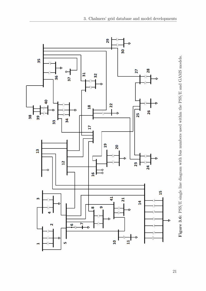
3.1 12 kV grid at Chalmers. . . . . . . . . . . . . . . . . . . . . . . . . . 163.2 Load profile methodology flowchart . . . . . . . . . . . . . . . . . . . 173.3 Overview of Chalmers grid within the Microscada system. . . . . . . 183.4 Estimated and measured load profile at bus 07:11B 13/5-2016 . . . . 193.5 Measured voltages 13/5-2016 . . . . . . . . . . . . . . . . . . . . . . . 203.6 PSS/E single line diagram with bus numbers used within the PSS/E

and GAMS models. . . . . . . . . . . . . . . . . . . . . . . . . . . . . 213.7 Normalized solar output profile . . . . . . . . . . . . . . . . . . . . . 243.8 Irradiance data for Landvetter Göteborg . . . . . . . . . . . . . . . . 253.9 Load profile . . . . . . . . . . . . . . . . . . . . . . . . . . . . . . . . 263.10 Load scaling factor for the extended microgrid model. . . . . . . . . . 273.11 Flowchart of the microgrid simulation platform . . . . . . . . . . . . 31

4.1 Flowchart of storage system design methodology . . . . . . . . . . . . 364.2 Benefits of battery storage for one year, displayed for different ESS

sizes . . . . . . . . . . . . . . . . . . . . . . . . . . . . . . . . . . . . 384.3 Benefit to investment cost ratio for different amount of installed storage. 394.4 Benefit to investment cost ratio for different interest rates and ex-

pected lifetimes of storage. . . . . . . . . . . . . . . . . . . . . . . . . 394.5 Benefit to investment cost ratio for different battery prices. . . . . . . 40

5.1 Power bought from the grid when EMM is used including ESS andwithout EMM. . . . . . . . . . . . . . . . . . . . . . . . . . . . . . . 43

5.2 Island mode operation with two 1-hour outages . . . . . . . . . . . . 445.3 Benefits to investment cost ratio for different ESS sizes, with varying

amount of installed solar power. . . . . . . . . . . . . . . . . . . . . . 455.4 Total cost for one year vs number of EVs. . . . . . . . . . . . . . . . 465.5 Output power PEV and SOC during one day of operation. . . . . . . 475.6 Island mode operation time for different ESS sizes with 3 MWp solar

PV installed . . . . . . . . . . . . . . . . . . . . . . . . . . . . . . . . 48

xiii

List of Figures

5.7 Total energy cost compared to base case for different configurationsincluding battery storage, solar power and EVs. . . . . . . . . . . . . 49

A.1 Load data for all buses in Chalmers grid 17/3-2016 . . . . . . . . . . XIIIA.2 Load data for all buses in Chalmers grid 17/3-2016 . . . . . . . . . . XIV

xiv

List of Tables

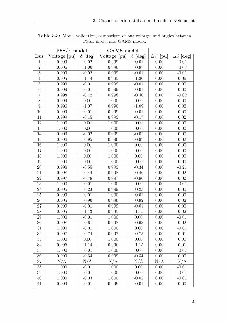
3.1 Branch Data . . . . . . . . . . . . . . . . . . . . . . . . . . . . . . . . 223.2 Transformer Data . . . . . . . . . . . . . . . . . . . . . . . . . . . . . 233.3 Model validation, comparison of bus voltages and angles between

PSSE model and GAMS model. . . . . . . . . . . . . . . . . . . . . . 33

4.1 Total cost for one day with different ESS locations . . . . . . . . . . . 37

5.1 Total energy cost for 24-hours for normal operation and with two1-hour outages. . . . . . . . . . . . . . . . . . . . . . . . . . . . . . . 44

5.2 Comparison of different investment costs, annual revenues and islandmode operation times for different ESS and solar PV sizes . . . . . . 47

A.1 Load profile for each hour of a day, 17/3-2016 . . . . . . . . . . . . . XII

xv

List of Tables

xvi

List of Abbreviations

CF Voltage Correction Factor.

CHP Combined Heat and Power.

CRF Capital Recovery Factor.

DER Distributed Energy Resources.

DNI Direct Normal Irradiance.

EMM Energy Management Model.

ESS Energy Storage System.

EV Electric Vehicle.

GAMS General Algebraic Modeling System.

MSP Microgrid Simulation Platform.

NRMSE Normalized Root Mean Square Error.

OPF Optimal Power Flow.

PCC Point of Common Coupling.

PSS/E Power System Simulator for Engineering.

PV Photovoltaics.

RES Renewable Energy Sources.

SAM System Advisor Model.

SOC State of Charge.

V2G Vehicle to Grid.

xvii

List of Abbreviations

xviii

List of Symbols

B Susceptance.

CESS Total cost of energy storage system.

Erated Rated energy capacity of batteries.

Elprice Electricity spot market price.

E Energy.

GCCHP Generation cost for CHP.

G Conductance.

I Current.

PF Penalty factor associated with load curtailment.

PCHP Power output from CHP.

PLoad,est Estimated power.

PLoad,meas Measured load.

Pbattery Active power output from batteries.

Pchr Charge power from storage.

Pdis Discharge power form storage.

Pfan Ventilation power.

Pflex Flexible active load.

Pgrid Power from the main grid.

Pload Active power load.

xix

List of Symbols

Ppv Active power from solar PV.

Psolar,rated Rated power output for PV.

Psolar Normalized power output from PV.

Qflex Flexible reactive load.

SF Scaling factor for load profile.

V Voltage.

∆Pload Active load regulation.

∆Qload Reactive load regulation.

cos(φ) Power factor.

ηchr Charge efficiency.

ηdis Discharge efficiency.

θi,j Voltage angle between bus i and j.

h Hour h.

i Bus i.

m Number of days.

xx

1Introduction

1.1 Background and Motivations

There are several reasons small-scale Distributed Energy Resources (DER) are beingmore and more utilized within the distribution grid. A more liberated energy market,higher demand for reliable electric power and new policies regarding environmentalfriendly power are major factors for this increase [1]. DERs include wind power,solar Photovoltaics (PV), the Electric Vehicle (EV) fleet etc. The distribution gridoperator is then faced with a great challenge when trying to operate and control thesystem. A microgrid aims to help the operator with these issues.The microgrid consists of locally grouped generation, storage and load within thedistribution grid. The local energy resources can be operated to supply the localdemand in the most beneficial way. A microgrid can also be disconnected from thedistribution grid and be operated independently from the main grid, in the so calledisland mode. Operating a grid as a microgrid gives more control over the DERsto the microgrid operator and it is easier to include new DERs which might leadto a more economically beneficial operation of the system. The reliability is alsoincreased since the microgrid can be operated independently of the main grid.There are several challenges when implementing a microgrid. It is important to havea reliable power quality by controlling the voltage and the frequency, which is difficultwhen many small-scale DERs are used. There is also a need for a sufficient controlstrategy when the microgrid is operated in island mode in order to keep the systemoperational. Additional challenges comes in the form of protection requirements andeconomical challenges [2].The internal grid at Chalmers has a lot of similarities with a microgrid. It is a clearlydefined area with some generation in the form of a Combined Heat and Power (CHP)unit and solar PV. The CHP plant has an electrical power output of maximum 1MW while the solar PV is rated at 15.7 kW. There are also EVs used at Chalmerswhich can represent distributed energy storage, although they are not used for thispurpose at the moment. Together, the local generation and energy storage couldpossibly be used to operate part of Chalmers’ grid as an autonomous microgrid.The ventilation at Chalmers also has down regulating possibilities, where the total500 kW of ventilation load can be down regulated by approximately 20% if needed.The interest to develop microgrids at Chalmers is strong and it is therefore valuableto evaluate how operating Chalmers’ grid as a microgrid would benefit the gridowner as well as the grid users. To evaluate and further study the benefits ofrunning Chalmers’ grid as a microgrid, there is a need for a model of the internal

1

1. Introduction

grid at Chalmers, including the grid data and load profiles for all buses. Alterationsin the microgrid, such as increased PV capacity, is also important to evaluate to seewhich benefits the grid operator could possibly receive.

1.2 ObjectivesThe objectives of this project include:

• Development of a database for the consumption load profile and grid data forthe Chalmers’ electrical grid

• Development of an Energy Management Model (EMM).• Determining the best location and size of battery energy storage for Chalmers’

microgrid using a cost-benefit analysis approach based on the EMM.• Performing a benefit assessment for operating the microgrid for various case

studies on PV capacity and EV usage using the developed EMM.

1.3 Specific tasksIn order to achieve the projects’ objectives, the thesis is divided into three specifictasks. An overview of these tasks can be seen in Figure 1.1.

Figure 1.1: Overview of the tasks

Task 1. Load profile and data collection/measurements

Knowledge about the grid and load profiles are necessary to create a model of theinternal grid at Chalmers. This needs to be measured in order to acquire datawhich can be used to obtain accurate and relevant simulations. This task will aim

2

1. Introduction

to measure and develop a database of the load profile within Chalmers’ grid, as wellas data on the internal generation and energy storage units present in the grid.

Task 2. Development of energy management model

In order to simulate the Chalmers’ grid a model of it must first be developed. Thismodel will be based on an Optimal Power Flow (OPF) framework which can be usedto schedule the local energy resources, which are the flexible loads, local generationand the energy storage. A cost-benefit analysis approach to determine how muchenergy storage is needed and where it should be placed will be developed. The OPFmodel, contains constraints such as power flow, flexible load and Energy StorageSystem (ESS) constraints. The model could be used to evaluate, for example, howthe system should be controlled to minimize the cost for the grid owner.

Task 3. Case study using the developed EMM

Several case studies for various configurations of Chalmers’ microgrid will be madebased on the developed EMM. A base case when the Chalmers’ grid is operatedas a microgrid will first be evaluated. Island mode operation, an increased amountof solar PV present in the grid and utilizing Vehicle to Grid (V2G) will also beevaluated. These case studies will provide a benefit assessment when running theChalmers’ grid as a microgrid.

1.4 ScopeThe project will consider the already existing grid at Chalmers with its currentlyinstalled power production (CHP and solar PV). Alterations to the grid will onlybe considered in the case studies and only in forms of increased generation. Theprotection system of the grid is assumed to be sufficient and changes in the protectionsystem as a result of the grid being operated as an autonomous microgrid will notbe considered. Energy storage in the microgrid will be taken into consideration,that is, location and size of energy storage to achieve a certain amount of time ofoperation for the Chalmers’ grid when disconnected from the main grid. The systemis considered in steady state, therefore transient studies will not be conducted. Thetime resolution of the model will be 1-hour, thus the model will be a planning modelsince a higher resolution would be necessary for controlling a microgrid.

1.5 Thesis outlineThe thesis consists of six chapters including the introduction. The chapters aresummarized below:

• Chapter 2 provides a technical background to the project, including previouswork on the subject of Microgrids.

• Chapter 3 handles the database development, model formulation and the struc-ture of the Microgrid simulation platform used in the project.

3

1. Introduction

• Chapter 4 explains the cost-benefit analysis which has been performed to findthe optimal energy storage from an economical point of view. It also presentsresults of simulations to obtain the optimal energy storage size and location.

• Chapter 5 handles case studies which have been performed regarding Islandmode operation, increased renewable energy generation and implementationof V2G with electric vehicles in the microgrid. The case studies are explainedand their results are presented.

• Chapter 6 consists of a conclusion of the thesis and some proposals of futurework.

4

2Technical background

This chapter aims to discuss the theory behind the microgrid concept, its compo-nents and discussions about previous microgrid studies. The chapter also discussesdifferent energy storage possibilities and features of a microgrid.

2.1 The microgrid conceptThe microgrid concept revolves around the use of local energy resources, such asgeneration and storage, to supply a local demand, thus forming a smaller grid withinthe main grid. This smaller grid is viewed as a subsystem to the main grid withits own control system and is connected at the Point of Common Coupling (PCC).This allows for individual scheduling of local generation and load which in turn canlead to a lower operating cost for the microgrid. An overview of a general microgridlayout is illustrated in Figure 2.1 [3].A microgrid can be operated both in conjunction with and independently of themain grid provided enough local generation and storage is present to supply thedemand. The option to run independently from the main grid, so called islandmode, will increase reliability for the microgrid since it can be operational during afault in the main grid. Microgrids can also disable non essential loads during maingrid faults and load peaks in order to prevent local failure and thus keeping thesystem operational [4].There are economical aspects to the microgrid concept, in the way that it could po-tentially be beneficial to transform a small section of the main grid into a microgrid.Since a microgrid is locally controlled, the local energy resources can be scheduledto operate in such a way so the energy cost is minimized. One such energy resourceis an ESS, which can be charged during low market price and discharged duringhigh market prices thus lowering the operational cost of the microgrid.Small scale local energy resources can easily be implemented in a microgrid as longas sufficient control schematics are in place. This can in turn be used to achieve ahigh renewable penetration by including for example solar and wind power withinthe microgrid. These types of energy resources can also lower the operating costsince they provide energy from free resources when they are in place [3].There are several challenges to the microgrid concept which needs to be dealt withbefore it can be widely implemented. A local control system which makes surethe voltage and frequency fulfill the power quality standards needs to be in place.There are also synchronization issues when connecting to the main grid after beingoperated in island mode. Another issue with microgrids is the need for ESS which

5

2. Technical background

Figure 2.1: A conceptual microgrid with DERs and energy storage

comes with a high investment cost which might exceed the benefits for creating amicrogrid, thus making it inefficient from an economical point of view [5].

2.2 Key components of a typical microgrid

This section treats the key components usually present in a microgrid. This includesgeneration and storage technologies.

2.2.1 Electrical distribution grid

The most key component to a microgrid is having an electrical distribution gridwhere part of it can be transformed into a microgrid. The microgrid does notinclude the transmission grid but simply a portion of the distribution grid, whereDERs and energy storage can be included to form a microgrid. The distributiongrid forms the role of distributing power to the end customers, for example feedingindustries or facilities.

6


2.2.2 Distributed power generationThere are several different methods to generate power within the power grid. How-ever, only small scale energy resources is appropriate in a microgrid since the localenergy demand usually is small in a microgrid. At Chalmers there is currently aCHP-plant and solar PV installed which are both suitable energy resources in amicrogrid.

2.2.2.1 Combined heat and power

Combined heat and power is a method of creating heat as well as electric powerwithin the same plant. CHP systems deliver the majority of its output energyas heat with a smaller portion of electrical energy. This can be accomplished bythe utilization of a stream turbine where high pressured steam is forced througha turbine which is connected to a synchronous generator. The generator producesthe electrical part of the generated power. The heat is extracted in the form of hotwater which comes from low-pressure steam utilization in heat exchangers [6]. Thisprocess is illustrated in Figure 2.2.

Figure 2.2: Working principle of CHP

2.2.2.2 Solar Photovoltaics generation

Photovoltaics technology, or solar cells, can be used to generate electricity fromsolar irradiation. Since solar cells are possible to mount on top of buildings theycould be a suitable technology for microgrids where the area available for generationunits could be limited. Another benefit of solar PV is the fact that it can be easilyscaled by simply increasing the amount of solar cells to obtain the desired powergeneration. The general working principle of solar photovoltaics is shown in Figure2.3. If there are any DC loads such as battery storage, the energy from the solarpanels can be directly transferred to the battery storage instead of going throughthe conversion process shown in 2.3 to supply the AC loads.

7


Figure 2.3: Working principle of solar PV

2.2.2.3 Wind power

Wind power is a renewable energy resource which can be implemented in a microgrid.In a similar matter as solar power, the generation is dependent on weather conditionsand can therefore not be relied on to produce a constant power output. Wind powercomes with a downside of creating noise which can be disturbing depending onthe location of the microgrid. Although Wind power is currently not included inChalmers grid it is a possible DER to be used within microgrids.

2.2.3 Energy storageEnergy storage is an important part of the microgrid system. It serves severaldifferent purposes such as frequency regulation, reliability improvement, peak powershaving and energy management applications leading to a lower cost for the system.The main purpose of energy storage is different depending on the conditions themicrogrid is operated under. In a microgrid with high amounts of Renewable EnergySources (RES), that are unreliable by nature, the energy storage systems are mainlyused to improve the reliability of the system by storing excess power when availableand supplying it when the power production is low.In a microgrid without sufficient generation to operate independently, the storagecan be used to achieve operation in island mode for a certain amount of time. It canalso be used for peak power shaving in all types of microgrids making the systemmore economical to operate. Energy storage may also simplify black starting of themicrogrid since the energy stored can be supplied to the grid during this event [7].The energy storage can be constructed in either an aggregated manner or as adistributed energy storage system. The difference between the two is that the ag-gregated ESS has all the storage placed at the microgrid terminal so that the powerflow to the microgrid can be controlled at the point of common coupling (PCC)while in a distributed ESS the storage is spread out between different generationunits within the microgrid. The distributed ESS enables optimization of storagedepending on generation type.

8


2.2.3.1 Batteries

Batteries are a well known way of storing electrical energy and has been used fora long time. There are different types of batteries, such as Lead-acid, Sodium-Sulfur (NaS), Nickel-Cadmium (NiCd), Nickel-MetalHydride (NiMh) and Lithium-ion (Li-ion) batteries. The efficiency of battery storage can be estimated to 60-80%depending on type and depth of discharge. There are several aspects to factor inwhen choosing a battery type, such as price, energy density, power density and howenvironmental friendly the batteries are [7]. The advantages of li-ion batteries comesin the form of high power and energy density but with the drawback of having arelatively high cost [8]. When looking at battery storage for microgrids, it is shownthat the discount rate used for economical analysis influences which battery typeis the most suitable. For discount rates above 4% li-ion is shown to be the mostcost effective battery storage alternative [9]. The investment cost for batteries hasdeclined by 8% annually and was around 300$/kWh in 2015 [10]. Since the EVindustry is growing, the need for better and cheaper batteries is growing with it.For EVs to be cost competitive with the classical combustion vehicles the batterycost need to be lower than 150 $/kWh [10]. Out of all commercially availible batterystorage technologies, the Li-ion battery is the best choice for high power and highenergy applications [3].

2.2.3.2 Vehicle to grid (V2G)

The concept of V2G is based on the energy stored in the EVs. Electric vehiclescan be of different types, such as plug in hybrid EV, fuel cell EVs and battery EVs.For hybrid EVs and battery EVs, the energy is stored in batteries, and for batteryEVs a connection to the grid is required for charging. Electric vehicles that aregrid connected enables the energy stored in the batteries to be supplied to the grid.Vehicle to grid is thereby a type of battery energy storage which can be used formicrogrid applications [11].With an increasing amount of EVs, possibilities in generation are increasing. Forthe USA, assuming a car fleet consisting of 25 % EVs the total power generation canbe estimated to 660 GW. It is shown that the vehicles are used about 4 % of thetime on average, meaning that the energy stored within the vehicles can possibly beused for other purposes such as V2G [12].

2.2.3.3 Flywheel

Flywheel energy storage is based on storing energy as kinetic energy within a flywheelwhich can then be converted to electrical energy though an electric machine whenneeded. Flywheels have a very short response time and are capable of delivering highpower levels. This makes them useful for protecting critical loads since they are ableto respond quickly and keep the system operating until other forms of generationcan be online. The lifetime of a flywheel is long compared to batteries and is almostindependent of the charge/discharge pattern. This allows for many charge cyclesand there is no need for periodic maintenance [13].The drawbacks with flywheels as a type of energy storage are the storage capability,

9


large size and high standby losses. This makes flywheels unsuitable for long timeenergy storage [7].In today’s grid, flywheels are used to protect critical loads, such as hospitals, fromsystem failures. They are able to prevent failures without additional generation inmost cases as 97% of all AC outages lasts for less than 3 seconds. However, forlonger failures other energy sources need to be activated in order to keep the systemoperational [14].

2.2.3.4 Supercapacitors

Supercapacitors (also know as ultracapacitors) operate under the same principles asregular capacitors in that they store energy by separating charge. However, superca-pacitors have a much higher capacitance for its size compared to regular capacitors.By separating the charge, the energy storage is made without the chemical processrequired by batteries thus supercapacitors can achieve a very fast response time [7].Supercapacitors have a high power density comparing to batteries and can thuscharge and discharge quickly. However, batteries can store more energy than asupercapcitor and also have a lower self-discharge rate when storing energy overlonger time periods [7], [15].It has been shown that supercapacitors have a high cycle lifetime, typically hun-dreds of thousands cycles, for a 100 % discharge depth. These advantages makessupercapacitors ideal when dealing with frequency control, transients and short-termstorage [15].

2.3 Features of microgridsThe benefits of running a section of a grid as a microgrid come in different forms. Forinstance, one can schedule the local energy resources in such a way that the operatingcost is minimized. This includes scheduling the use of ESS and controllable loads.Other benefits comes in the form of control over the grid and what energy resourcesthat can be included.

2.3.1 Demand responseThe principle of demand response is based on evening out the hourly demand ofpower. By shifting the demand from the demand peaks to off-peaks the total cost ofenergy can be lowered. This can be done by moving the controllable loads in timeto when the electricity price is lower thus reducing the total cost. Demand responsecan also be used in emergencies, for example in hospitals, to lower the total load byonly operating the essential loads and thus keeping the system operational [16]. Forindustrial users the price paid for electricity is also determined partly by the peakdemand of the facility, thus lowering the peak demand can further decrease the cost[17].In a grid with a high renewable penetration it could be beneficial to shift demand tohours where the generation is high. However, this might increase the peak demandwhich requires a higher capability system [16].

10


One way of implementing demand response in a local power system is to include anESS unit. The grid can then use the ESS as a generating unit when the demandis high thus lowering the total power provided by the main grid. The ESS willthen recharge when the demand is low in order to be ready for use during the nextdemand peak.

2.3.2 Energy management system in microgridsAn energy management system (EMS) is a software which controls the DERs, loadsand their scheduling within the microgrid. Knowledge about grid states and marketprices are necessary to schedule generation and load, therefore communication be-tween the EMS and generation and load units are necessary. The aim of the energymanagement system is to optimize the controls of load, generation units and powerflow [18]. This means that scheduling of units within the microgrid can be con-sidered an optimization problem, where the objective can be to minimize the totalenergy cost for example. The EMS is located within the microgrid central control(MCC) as shown in figure 2.1.

2.4 Previous WorkThis section discusses some previous work on the subject of microgrids, as well asexperimental microgrids that have been tested.

2.4.1 Sizing of Energy Storage SystemsSizing of energy storage systems designed for microgrid applications is relevant froma cost-benefit point of view. Determining the optimal size of the energy storageincludes considering the minimal size of the energy storage. The minimum size of thestorage depends on the application, but for island mode microgrids, the possibilityof running the microgrid independently must be considered. With the objective ofminimizing the total cost for an island mode microgrid and maximizing the totalbenefits for a grid-connected microgrid a study was made resulting in two modelswith the aim of finding a solution to both objective functions [19]. These methodsaims to find the optimal size for both island mode and grid connected operation. Thesolver used was a MILP solver and the method aims to evaluate different storage sizesbetween a chosen minimum and maximum size and find which the most beneficialsize is. The study shows that an optimal solution to sizing of energy storage existswhere the solution is different for grid-connected and island mode microgrids. Thestudy shows that the total cost could be reduced by 8.64% per day for the islandmode microgrid [19].Another method of finding the optimal size of energy storage could be to utilizegenetic algorithm (GA) which has been used for unit commitment and other powersystem problems. GA is based on natural evolution and natural selection, andthere is a probabilistic approach to the solution. The benefits of using GA is thatit provides several solutions, and that the iterative search of an optimal solutionis conducted over a population of solutions rather than one [20]. There is also a

11


method called multiobjective particle swarm optimization (MOPSO) which can beused to solve problems including several objectives [3].

2.4.2 Experimental MicrogridsTesting of the microgrid technology has been conducted in several places over theworld, where evaluation of its functionality has been done.

2.4.2.1 CERTS testbed US

The CERTS testbed was built near Columbus Ohio US, where the microgrid conceptwas tested at a full scale with 3x60 kW generation units, each with an energystorage located at its DC bus. The aim of the project was to test the possibilityof a smooth transition between grid-connected and island mode, having a reliableprotection system and finally a stable system with regards to voltage and frequencyin both operation modes. The testing was found to fulfill all set goals regardingpower quality standards and the protection system and controls were found to befunctioning according to the set goals [21], [22].

2.4.2.2 University of Texas at Arlington microgrid testbed

The university of Texas at Arlington have developed and constructed a microgridtestbed used for research purposes. It consists of three different microgrids placed ina ring layout which allows them to operate separately or together with each other.This allows for simulations on how microgrids can help support other microgridsand thus increasing the reliability of the local power system.The microgrids consists of solar PV, wind turbines and an ESS. There is also a fuelcell installed in one of the three microgrids and a diesel generator located at thePCC. Each grid is equipped with a flexible load and can further be equipped withconventional loads if deems necessary [23].

2.4.2.3 Microgrid design considerations for Eindhoven University of Tech-nology campus

The transitioning of a university campus grid into a microgrid was considered, wherethe goal was to propose a design of said microgrid [24]. The consumption of thecampus grid was 52 GWh excluding the natural gas consumption of 79 GWh. Therewas also an already existing thermal energy storage of 20 MWt which in the thesisis assumed to be increased to 30 MWt. There is also a planned installation of 10.5MWp of solar PV to supply the electrical load at the campus. It is concluded thatthe RES are producing a power surplus for 220 hours of the year, meaning thatthis surplus could be exported or stored within the microgrid. Both mobile storagein the form of vehicles and battery storage are also considered within the grid forsimulations. The battery storage is assumed to consist of Li-ion batteries with a costof 500 €/MWh, and a lifetime of 15 years. To ensure the lifetime the State of Charge(SOC) is limited between 0.2 and 0.8. Simulations show that it is only beneficial toinclude battery storage for limited sizes. It is concluded that battery storage is not

12


beneficial with the investment cost and electricity prices used from 2014. However,with higher electricity prices and cheaper batteries the battery storage is consideredto have future potential [24].

2.4.3 Economic analysis of microgrid including EVs

A study from 2011 was conducted regarding the economic benefits of a microgridincluding EVs as part of its generation [25]. The study was conducted by simulationsusing particle swarm optimization which is an iterative optimization method, toschedule the unit commitment within the microgrid. The power flow is bidirectionalin the study meaning that the EVs are used for both injecting and taking power fromthe microgrid. The microgrid studied has an electrical demand of 5.9 GWh/yearand a peak demand of 950 kW. The control strategy of EVs is based on generationexcess or deficit. When the total generation within the microgrid is greater than theload, the energy is stored within the batteries of EVs and when the generation isless, the batteries of the EVs is used to inject power to the microgrid. The electricvehicles are assumed to have a SOC of 73% when owners arrive at the office. TheSOC is limited to not go below 33% during the day. By the proposed contract themicrogrid owner and the car owners share the benefits obtained by including EVsin the microgrid. The operational cost of the grid is shown to decrease by 5.02%which is the benefit seen by the grid owner. The car owners get their benefit from aconnection payment which is suited to compensate for battery degradation. Batterydegradation is increased due to the charging cycles taking place within the microgrid.The study concludes that it is beneficial for both car owners and microgrid operatorto include EVs as a part of the microgrid [25].

2.4.4 AC and DC microgrids

Since the main grids around the world are dominated by an AC infrastructure itis easy to implement AC in the microgrids. As more and more power sources thatgenerate DC power are utilized, DC microgrids become more and more attractive.However, the DC technology needs to mature before it can be used as a reliablepower system [26].

2.4.4.1 DC microgrids

The reasons why DC microgrids could be a valid option to AC microgrids are several.Many of the customer loads of today are DC powered, and the increase in renewableenergy sources is another reason why DC microgrid could be viable. Solar PV andfuel cells are naturally producing DC power, thus it is more efficient to utilize themin a DC grid. Regarding other RESs such as wind turbines, they are often connectedto the AC grid via a DC-link, thus by cutting out the conversion stage the efficiencycould be increased [27]. There are also challenges associated with DC microgrids,such as protection. It is challenging to construct a protection system for DC sincethere is no natural zero crossing in DC current [27].

13


2.4.4.2 AC microgrids

The more conventional AC grid is dominant as of today due to its efficient transfor-mations in voltage level, and also due to fossil fueled generation being well suited forAC [28]. Since a microgrid is often aimed towards including RES, these need to beconnected to the grid. Solar PV is naturally producing DC current thus conversionis needed in order to connect them to an AC grid. On the other hand, with in-creasing amounts of local RES the need for long transmission lines could be reducedin the future [28]. Protection systems can easily be adapted from todays AC gridstandards into a microgrid. The case is the same regarding frequency and voltagecontrol, thus making the transition somewhat simple [29].

2.4.4.3 Hybrid microgrid

A study on a hybrid AC/DC microgrid was made in 2011 [28]. This study proposesthe use of a AC/DC microgrid to minimize the AC to DC transformations in thegrid. An investigation on a hypothetical microgrid consisting of 40 kW PV connectedto the DC side, 50 kW wind connected to the AC side and a variable load of 20-40kW connected on both sides of the microgrid. The study evaluates the stability ofthe microgrid in both grid connected and island mode operation.It is concluded that the hybrid AC/DC microgrid proposed offers satisfactory sta-bility both when operated in grid connected and island mode. However, due to theAC infrastructure of the main grids, it is difficult to apply a AC/DC microgrid intoday’s society [28].

14

3Chalmers’ grid database and

model developments

This chapter describes how the database for the Chalmers’ electrical grid and themicrogrid simulation platform are developed. The database consists of network data,which was provided by Akademiska Hus, and load data which was taken from differ-ent measurements to create load profiles for the grid. These load profiles are thenused as input in the EMM which was developed using General Algebraic ModelingSystem (GAMS) software. The objective of the EMM is to minimize the total en-ergy cost of the system and it is solved with constraints such as power flow equations,network constraints and ESS constraints. The simulated results are then validatedby comparing acquired voltages from the grid model to values taken from PSS/Esoftware.

3.1 Database developmentA database has been developed consisting of load profiles of the Chalmers grid, gridand generation data. The 12 kV chalmers grid is presented in figure 3.1, howeverthe loads connected to each transformer in the grid were unknown hence a databasewith this information needed to be developed.The system consists of of 22 buses of which 17 are load buses. Connection to themain grid is located at bus 07:8 and the CHP plant is located at bus 07:8.1.1, bothwithin the building Kraftcentral. There is also solar PV located at bus 07:8.1.1 notshown in the single line diagram. A backup connection to the main grid is connectedto bus 07:35, however, this bus is normally disconnected and is therefore not usedin any simulations.

3.1.1 Load DataIn order to create a database of the different loads within the Chalmers grid threedifferent methods to collect data have been used. These are own measurements ata substation, the energy usage in all the buildings measured by Akademiska hus,responsible for the power grid at Chalmers, and current measurements taken fromMicroscada, also provided by Akademiska hus. By combining these measurements,an accurate load distribution have been created.Akademiska hus provided a database with the energy consumption within eachbuilding for each hour of the day for 2015. This database gives a picture of how

15

3. Chalmers’ grid database and model developments

Figure

3.1:12

kVgrid

atChalm

ers.

16


the energy demand varies during the day but since not all buildings have their ownsubstations, these values can not readily be inserted into the model. Thereforecurrents from Microscada are included to construct the load profiles.Microscada is the software used to monitor the grid within Chalmers and can alsobe used to monitor the currents within the system. These currents can then beused to calculate the power demand at the substations within the system. However,not all currents are being measured so complementary data has been taken fromAkademiska hus database. By comparing the energy consumption data over theyear, a scaling factor is determined which is then used to extend the 24-hour loadprofile to be valid for an entire year. The methodology of constructing the loadprofiles is shown in Figure 3.2.

Figure 3.2: Load profile methodology flowchart

The estimated load power, PLoad,est, for each node i in the grid at every hour h isexpressed in Equation 3.1. The voltage V is assumed to be 1 p.u, the load powerfactor cos(φ) is assumed to 0.98 and the current I is taken from Microscada.

PLoad,est(i, h) =√

3|V (i, h)||I(i, h)|cos(φ) (3.1)

3.1.2 MeasurementsMeasurements have been conducted in substation 07:11B located in the EDIT-building. The voltage, current, power output and power factor have been monitoredfor half a day between 07:00 and 17:00. These measured values are then used tovalidate and improve the load profile. By comparing the load profile obtained bythe estimation, PLoad,est, and the actual measured values, PLoad,meas, the NormalizedRoot Mean Square Error (NRMSE) ,as described by Equation 3.2, can be calculated.

NRMSE =

√1n

∑nh=1(PLoad,meas(h)− PLoad,est(h))2

PLoad,meas

(3.2)

The voltage is measured which in the estimated value of the load is assumed to 1p.u. By defining a Voltage Correction Factor (CF) as described in Equation 3.3 the

17


Figure

3.3:Overview

ofChalm

ersgrid

within

theMicroscada

system.

18


model can be refined.

CF = Vmeasured(h)Vestimated(h) (3.3)

where Vmeasured is the mean value of the measured line-to-line voltages and Vestimated

is the assumed constant voltage of 400V line-to-line.The results of the measurements are presented, where the voltages, currents andactive power have been measured during half a day, with 1-hour resolution. Figure3.4 shows the estimated and measured load profiles. It is visible that the two profilesare similar although some differences are seen. These might be due to measurementspoints being hourly, meaning that the instantaneous values of power differ from themean power over the actual hour. The voltages shown in Figure 3.5 are experiencingsmall variations between 404 and 394 voltage, where the voltage is decreasing duringhigh demand hours.

6 7 8 9 10 11 12 13 14 15 16 17

Hour

0

50

100

150

200

250

300

350

400

Active

Po

we

r [k

W]

Estimated load profile

Measured load profile

Figure 3.4: Estimated and measured load profile at bus 07:11B 13/5-2016

The NRMSE was calculated to 6.83%, and with the correction factor CF account-ing for the voltage difference this error was reduced to 6.71%. This suggests thatthe cause of the error is not the assumption of 1 p.u voltage level. The fact thatmeasurements were conducted taking one value per hour might affect the resultssince variations during each hour are not taken into account, thus it could be apossible cause of the error. Errors in current monitoring by Microscada could alsobe affecting the result.

19


7 8 9 10 11 12 13 14 15 16 17392

394

396

398

400

402

404

Hour

Vo

lta

ge

[V

]

L1

L2

L3

Figure 3.5: Measured voltages 13/5-2016

3.1.3 Grid data

The data required to create models of the network are acquired from AkademiskaHus. The data consists of cable dimensions, lengths, types of cables and transformerdata such as ratings and impedance values. These data are necessary to construct anaccurate model of the grid which is necessary in the optimal power flow calculations.The branch data for the network is shown in Table 3.1 and the transformer dataare shown in Table 3.2. Note that the transformers do not have any resistance andare thereby assumed to be lossless. The bus numbers are according to the modeldeveloped in PSS/E which can be seen in Figure 3.6.

3.1.4 Generation data

There are currently three types of generation available in Chalmers’ grid. These arepower from the main grid and local generation with the CHP plant or the solar PV.

From grid

When operated under normal conditions Chalmers’ grid receives power from themain grid operated by Göteborg Energi. This connection is seen as an endlesspower supply from the microgrid and can be bought using Nordpool day-ahead spotmarket prices [30].

20


Figure3.6:

PSS/

Esin

glelin

ediagram

with

busnu

mbe

rsused

with

inthePS

S/E

andGAMSmod

els.

21


Table 3.1: Branch Data

From bus- To bus

Line-length [m] R [mΩ] X [mΩ] Line-

charging [µF ]Current-limits [A]

1-3 75 9.4 6.4 0.030 3851-5 70 8.8 5.9 0.028 3855-6 40 7.0 3.4 0.014 3005-12 275 34.4 23.3 0.11 3855-41 250 14.4 6.4 0.0245 3858-17 110 13.8 9.3 0.0440 38510-41 100 20.6 9.3 0.035 30012-13 25 1.6 1.1 0.005 77012-16 15 1.9 1.3 0.006 38512-17 20 2.5 1.7 0.008 38512-18 25 3.1 2.1 0.010 38513-14 420 52.5 35.6 0.168 38516-19 25 3.1 2.1 0.010 38517-31 330 41.3 28.0 0.132 38517-33 80 10.0 6.8 0.032 38518-23 225 28.1 19.1 0.090 38518-35 400 50.0 33.9 0.16 38523-25 300 37.5 25.4 0.12 38525-27 165 20.6 14 0.066 38529-35 400 51.3 34.8 0.164 38535-38 10 1.3 0.9 0.004 38538-39 25 4.0 1.2 0.004 205

CHP plant

The CHP plant at Chalmers has a maximum electrical output power of 1 MW. Toproduce this amount of power there will also be heat generated, which has to beeither used or sold. The cost of generation of the CHP plant, GCCHP , is estimated to600 SEK/MWh according to Akademiska Hus, not taking into account the benefitsof possibly selling the produced heat.

Solar PV

A solar PV panel with a rated power of 15.7 kW is installed at a wall at Chalmerswhich is a part of the local generation and is assumed to have no cost associatedwith it. Two different methods have been used to get the power output from thissolar PV depending on the time span the simulation is run for.

Short-term solar estimation

When the simulations are run for the short-term, 24 hours are considered. Theoutput power profile seen in figure 3.7 is then used for estimate the solar poweroutput and is a normalized output profile for three days during spring 2016, 22th

22


Table 3.2: Transformer Data

From-To X [%] Rating [kVA]1-2 4.8 8001-2 5.0 8001-2 5.2 8003-4 5.69 8006-7 5.8 10008-9 5.8 80010-11 4.82 80014-15 5.0 125014-15 5.0 125014-15 4.9 125018-22 5.5 125019-20 6.31 80019-20 5.0 80021-41 5.7 80021-41 6.3 100023-24 4.27 40025-26 4.8 80027-28 4.9 80029-30 5.8 80031-32 4.5 125033-34 6.3 80033-34 6.3 80035-36 5.2 80035-36 4.9 60039-40 5.2 125039-40 5.2 1250

of february, 30th of april and 12th of may. The data for these days is based ona 5.5 kW rated solar farm located in Gothenburg. It can be seen that the day inApril is poor in solar irradiation while the day in February is a sunny day, thus thebig difference between the two. The power output is calculated using equation 3.4where Ppv is the output power from the solar cells, Psolar is the power output forhour h from figure 3.7. Psolar,rated is the rated power of the solar panels.

Ppv(h) = Psolar(h) · Psolar,rated (3.4)

Medium-term solar estimation

Due to limitations in the data available from the solar panels used for the short-termmodel, the total beam irradiance is instead used to estimate the output power ofthe solar panels when the medium-term model is ran. The irradiance data is takenfrom System Advisor Model (SAM), which is a model software which also consists

23


0 5 10 15 20

Hour

0

0.2

0.4

0.6

0.8

1N

orm

aliz

ed

Po

we

r O

utp

ut

22 Feb

30 Apr

12 May

Figure 3.7: Normalized solar output profile

of a database with for example irradiance data. An irradiance profile for an averageday for each month of the year is used to estimate the power output of the solarpanels, giving a model which accounts for the changes in irradiation over the year.The irradiance data is presented in figure 3.8, where the Direct Normal Irradiance(DNI) for four months of the year is shown.The power output of the solar cells is estimated using equation 3.5 where DNIST C

is the irradiance used for standard test conditions to calculate the rated power ofsolar cells, which is 1000 W/m2 according to IEC 60904-3 [31]. DNI(h) denotes theirradiance for each hour as shown in figure 3.8 and Prated is the rated power of theinstalled solar cells.

Ppv(h) = DNI(h)DNIST C

· Prated (3.5)

3.1.5 Load profilesTwo different load profiles have been developed, one for the short-term model andan extended load profile for the medium-term model.

Short-term model

The simulations have been carried out based on a load profile for Thursday 17th ofmarch 2016. This profile can be seen in table figure 3.9. It can be observed thatthere is a higher demand during the workday and the peak of 5472.9 kW occurs athour 14. The total energy demand for 24 hours is calculated to be 105.5 MWh.

24


0 10 20 30

Hour

0

100

200

300

400

500D

ire

ct

No

rma

l Ir

rad

ian

ce

[W

/m2

]January

0 10 20 30

Hour

0

100

200

300

400

500

Dire

ct

No

rma

l Ir

rad

ian

ce

[W

/m2

]

May

0 10 20 30

Hour

0

100

200

300

400

500

Dire

ct

No

rma

l Ir

rad

ian

ce

[W

/m2

]

September

0 10 20 30

Hour

0

100

200

300

400

500

Dire

ct

No

rma

l Ir

rad

ian

ce

[W

/m2

]

December

Figure 3.8: Irradiance data for Landvetter Göteborg

Medium-term model

To extend the load profile to be valid for the medium-term model, which has a timespan of one year, the load profile presented for the one-day model was scaled with afactor based on the energy consumption variations over the year. This scaling factoris calculated by comparing the energy consumption for all buildings with the onesduring the day which the short-term load profile was extracted. The scaling factorSF is then expressed as in equation 3.6.

SF (h) = E(h, d)E(h, 76) (3.6)

where day 76 denotes the example day used for the one-day model.The load is then estimated according to equation 3.7.

Pload(i, h, d) = Pload(i, h, 76) · SF (h) (3.7)

This load scaling factor is presented in figure 3.10. It is shown that the load isreduced during the summer when the activity at campus is naturally lower. Thevariations between days is due to weekends having a lower energy consumption sincethere is no education being held at weekends.

25


5 10 15 203

3.5

4

4.5

5

5.5

6

Hour

To

tal L

oa

d [

MW

]

Figure 3.9: Load profile

3.2 Modeling

The modeling consists of three models, one load flow model in PSS/E and twoOPF-based microgrid energy management models, one to simulate for one day andan extended model for one year simulations. The models consist of an optimizationmodel in GAMS [32] and data management in MATLAB.

3.2.1 Power flow in PSS/EA model of the network was constructed using Power System Simulator for Engi-neering (PSS/E) to visualize the network. The model includes grid data such asline impedance, transformer data and voltage levels. The PSS/E model is used torun a power flow with fixed values for loads to establish a base case for how the gridworks. The model can later be used to validate the results from the EMM.The one-line diagram of the PSS/E model is shown in Figure 3.6. It can be notedthat the PSS/E model has 41 buses which is more than the single line diagramprovided by Akademiska Hus. This is because extra buses are used to connect theload to the low voltage side of the transformers. Bus 13 is considered the slack bus ofthe system since this is the PCC where the main grid is connected to the microgrid.

3.2.2 OPF-based EMM for microgridsThe EMM model is constructed in GAMS to schedule generation and storage in themost efficient way based on the objective function which in this case is the total

26


0 1000 2000 3000 4000 5000 6000 7000 80000.2

0.4

0.6

0.8

1

1.2

1.4

1.6

1.8

Hour

Sca

ling

Fa

cto

r

Figure 3.10: Load scaling factor for the extended microgrid model.

cost of electricity for campus Johanneberg at Chalmers. The objective function isminimized with respect to several constraints due to the characteristics of the grid.The constraints consist of power flow equations, transmission constraints, generationand load constraints and finally constraints regarding energy storage such as SOCconstraints. Since some of the constraints are nonlinear the MINOS NLP (nonlinearprogramming) solver is used.

Objective Function

The objective function is expressed as seen in equation 3.8.

Cost =n∑

h=1

k∑i=1

PCHP (i, h)GCCHP (i) + Pgrid(i, h)Elprice(h) + PF∆Pload(i, h) (3.8)

where Elprice denotes the price from Nordpool day-ahead market for the grid powernot including taxes. Taxes and other grid costs where not accounted for due tounavailability of data. PCHP and GCCHP denotes the generation and its cost of thelocal CHP generation. Pgrid denotes the power injected by the main grid and PFdenotes the penalty factor associated with load curtailment. The penalty factor is afictive cost which is added in the objective function to control the load curtailment.This penalty factor determines when the flexible load should be activated so it isonly used the most beneficial hours. It is assumed to be 240 SEK/MWh, meaningthat the load curtailment will be activated only when the electricity price exceeds themean electricity price with 20%. ∆Pload describes the down regulation possibilities

27


at Chalmers which is estimated to 20% of the total ventilation power Pfan. Thetotal power of the fans is 500 kW and is assumed to be distributed according to loadlevels. It is described by equation 3.13.

Power flow equations

PCHP (i, h) + Pgrid(i, h)− [Pload(i, h)− Ppv(i, h)] + Pflex(i, h) =

=k∑

j=1|Vi||Vj|(Gi,j cos θi,j +Bi,j sin θi,j)

(3.9)

QCHP (i, h) +Qgrid(i, h)−Qload(i, h) +Qflex(i, h) =

=k∑

j=1|Vi||Vj|(Gi,j cos θi,j −Bi,j sin θi,j)

(3.10)

where G and B are the real and imaginary parts of the admittance between bus iand j respectively, θ is the voltage angle difference between bus i and j, Vi and Vj

are the voltages at bus i and j respectively. Pload is the static load for each hour hand bus i. [Pload-Ppv] denotes the residual load which is the total load Pload minusthe generated power from solar PV Ppv. Pflex is the flexible load which consists ofthe battery storage power Pbattery and regulating power ∆Pload.

Flexible load constraints

Pflex and Qflexcan be expressed as seen in equation 3.11 and 3.12.

Pflex(i, h) = ηdis · Pdis(i, h) + Pchr(i, h) + ∆Pload(i, h) (3.11)

Qflex(i, h) = Qbattery(i, h) + ∆Qload(i, h) (3.12)

where Pdis and Pchr is the power drawn or injected to the grid depending on chargingor discharging of batteries and ηdis is the discharging efficiency.

Down-regulating constraints

0 ≤ ∆Pload(i, h) ≤ 0.2Pfan(i, h) (3.13)

A change in active power ∆Pload also results in a change in reactive power ∆Qload

as described by equation 3.14

∆Qload(i, h) = ∆Pload(i, h) · tanφload(i, h) (3.14)

where φload(i, h) denotes the power factor. The power factor cosφload(i, h) = 0.98lagging, according to measurements from substation 07:11B which gives the powerfactor φload. Since the power factor is difficult to measure at all buses at the sametime is assumed to be constant for all buildings at Chalmers for every hour.

28


Generation and voltage constraints

The generation constraints sets the limit for the grid power and the CHP plantoperation. During normal conditions there are no constraints on the grid power ascan be seen in Equation 3.15 and 3.16.

Pgrid(i, h) ≤ ∞ (3.15)

Qgrid(i, h) ≤ ∞ (3.16)

The limitation on the CHP generation is given by

0 ≤ PCHP (i, h) ≤ PmaxCHP (3.17)

− 0.3 · PmaxCHP ≤ QCHP (i, h) ≤ 0.3 · Pmax

CHP (3.18)

where PmaxCHP is 1 MW.

The battery can act as both generation and load and the power output is limitedby the maximum power output of the batteries. This is seen in Equation 3.19, 3.20and 3.21.

Pchr(i, h) ≤ Pchr,max(h) (3.19)

Pdis(i, h) ≤ Pdis,max(h) (3.20)

− 0.3 · Pbattery,max(h) ≤ Qbattery(i, h) ≤ 0.3 · Pbattery,max(h) (3.21)

There are also constraints on the voltage levels within the grid which is seen inEquation 3.22.

Vmin(i) ≤ V (i) ≤ Vmax(i) (3.22)

where Vmin(i) is 0.95 and Vmax(i) is 1.05.

Power flow constraints

The apparent power limitations are implemented as a current limitation which isprovided by the cable manufacturer. The power limitation is described by equation3.23.

− Ilim(i, j) ≤ I(i, j) ≤ Ilim(i, j) (3.23)

3.2.3 Stationary battery energy storage systemThe ESS in the grid enables demand response as well as functioning as a backupgeneration in case of a disconnection from the main grid. The microgrid is assumedto be able to function for one hour in island mode, thus the minimum size of the

29


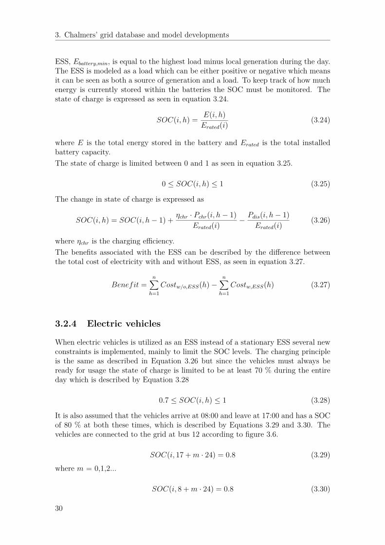
ESS, Ebattery,min, is equal to the highest load minus local generation during the day.The ESS is modeled as a load which can be either positive or negative which meansit can be seen as both a source of generation and a load. To keep track of how muchenergy is currently stored within the batteries the SOC must be monitored. Thestate of charge is expressed as seen in equation 3.24.

SOC(i, h) = E(i, h)Erated(i) (3.24)

where E is the total energy stored in the battery and Erated is the total installedbattery capacity.The state of charge is limited between 0 and 1 as seen in equation 3.25.

0 ≤ SOC(i, h) ≤ 1 (3.25)

The change in state of charge is expressed as

SOC(i, h) = SOC(i, h− 1) + ηchr · Pchr(i, h− 1)Erated(i) − Pdis(i, h− 1)

Erated(i) (3.26)

where ηchr is the charging efficiency.The benefits associated with the ESS can be described by the difference betweenthe total cost of electricity with and without ESS, as seen in equation 3.27.

Benefit =n∑

h=1Costw/o,ESS(h)−

n∑h=1

Costw,ESS(h) (3.27)

3.2.4 Electric vehicles

When electric vehicles is utilized as an ESS instead of a stationary ESS several newconstraints is implemented, mainly to limit the SOC levels. The charging principleis the same as described in Equation 3.26 but since the vehicles must always beready for usage the state of charge is limited to be at least 70 % during the entireday which is described by Equation 3.28

0.7 ≤ SOC(i, h) ≤ 1 (3.28)

It is also assumed that the vehicles arrive at 08:00 and leave at 17:00 and has a SOCof 80 % at both these times, which is described by Equations 3.29 and 3.30. Thevehicles are connected to the grid at bus 12 according to figure 3.6.

SOC(i, 17 +m · 24) = 0.8 (3.29)

where m = 0,1,2...

SOC(i, 8 +m · 24) = 0.8 (3.30)

30


3.2.5 Island mode constraintsTo be able operate the microgrid in island mode additional constraints on the ESSis required. The energy in the ESS must always be enough to supply the microgridfor the desired island mode operation time. The SOC limit is then updated withrespect of this required limitation as can be seen in equation 3.31

6 · tErated(i) ≤ SOC(i, h) ≤ 1 (3.31)

where t is the time of desired island mode operation in hours. For the worst casescenario, the ESS must supply 6 MWh to the grid for each hour the microgrid isoperated in island mode.

3.2.6 Microgrid simulation platformThe Microgrid Simulation Platform (MSP) is built up with both GAMS and MAT-LAB where all input and output data can be viewed and processed within MATLAB.The MSP structure is shown in figure 3.11. The reason for using both programs is thepossibility of changing input data and running numerous simulations with varyinginput in a simple way. The MSP consists of the MATLAB scripts, excel files con-taining input data and the EMM within GAMS. Other parameters such as storagelocation or size can also be altered from MATLAB.

Figure 3.11: Flowchart of the microgrid simulation platform

3.3 Short-term model (24-hour)When the EMM is run for a short-term time period, which is 24-hours, the suitableload profile and solar PV generation is used, as described in Section 3.1.5 and 3.1.4.The constraints used are Equation 3.8 to 3.27. The island mode simulations are alsomade using the short-term model and for those cases the Equation 3.31 replacesEquation 3.25.

3.4 Mid-term model (One year)The medium-term model, , which use a time period of one year, is used to evaluatethe optimal sizing of the ESS, as well as studying the behavior of the microgrid in amore detailed manner. This led to adjustments in load profile and solar PV power

31


which is described in Section 3.1.5 and 3.1.4. The same equations as in the short-term model are used, however, due to simulation difficulties the line constraints,given by Equation 3.23, are excluded. Due to complexity of running simulationsover the whole year at once, the model was designed to run the EMM for each monthindividually, thus running 12 separate simulations after each other to simulate anentire year.

3.5 Validation of load flow modelThe PSS/E model is used to validate the accuracy of the GAMS model. A snapshotof the power flow for one hour from the PSS/E model is used to compare the busvoltages and angles in the grid to the values obtained from the GAMS model whilerunning a power flow with the same load. The results are presented in figure 3.3.The results from the two simulations show that there is no difference in voltage levelsfor any bus and there are some slight difference for the voltage angle. The largestdifferences in angle occurs at bus 20 where the difference is −0.21 degrees. This ismost probably due to differences in the matter of solving the power flow equations.This shows that the EMM solves the power flow as intended.

32


Table 3.3: Model validation, comparison of bus voltages and angles betweenPSSE model and GAMS model.

PSS/E-model GAMS-modelBus Voltage [pu] δ [deg] Voltage [pu] δ [deg] ∆V [pu] ∆δ [deg]1 0.999 -0.02 0.999 -0.01 0.00 -0.012 0.996 -1.00 0.996 -0.97 0.00 -0.033 0.999 -0.02 0.999 -0.01 0.00 -0.014 0.995 -1.14 0.995 -1.20 0.00 0.065 0.999 -0.01 0.999 -0.01 0.00 0.006 0.999 -0.01 0.999 -0.01 0.00 0.007 0.998 -0.42 0.998 -0.40 0.00 -0.028 0.999 0.00 1.000 0.00 0.00 0.009 0.996 -1.07 0.996 -1.09 0.00 0.0210 0.999 -0.01 0.999 -0.01 0.00 0.0011 0.999 -0.15 0.999 -0.17 0.00 0.0212 1.000 0.00 1.000 0.00 0.00 0.0013 1.000 0.00 1.000 0.00 0.00 0.0014 0.999 -0.02 0.999 -0.02 0.00 0.0015 0.996 -0.95 0.996 -0.97 0.00 0.0216 1.000 0.00 1.000 0.00 0.00 0.0017 1.000 0.00 1.000 0.00 0.00 0.0018 1.000 0.00 1.000 0.00 0.00 0.0019 1.000 0.00 1.000 0.00 0.00 0.0020 0.998 -0.55 0.999 -0.34 0.00 -0.2121 0.998 -0.44 0.998 -0.46 0.00 0.0222 0.997 -0.78 0.997 -0.80 0.00 0.0223 1.000 -0.01 1.000 0.00 0.00 -0.0124 0.996 -0.23 0.999 -0.23 0.00 0.0025 0.999 -0.01 1.000 -0.01 0.00 0.0026 0.995 -0.90 0.996 -0.92 0.00 0.0227 0.999 -0.01 0.999 -0.01 0.00 0.0028 0.995 -1.13 0.995 -1.15 0.00 0.0229 1.000 -0.01 1.000 0.00 0.00 -0.0130 0.998 -0.61 0.998 -0.63 0.00 0.0231 1.000 -0.01 1.000 0.00 0.00 -0.0132 0.997 -0.74 0.997 -0.75 0.00 0.0133 1.000 0.00 1.000 0.00 0.00 0.0034 0.996 -1.14 0.996 -1.15 0.00 0.0135 1.000 -0.01 1.000 0.00 0.00 -0.0136 0.999 -0.34 0.999 -0.34 0.00 0.0037 N/A N/A N/A N/A N/A N/A38 1.000 -0.01 1.000 0.00 0.00 -0.0139 1.000 -0.01 1.000 0.00 0.00 -0.0140 1.000 -0.03 1.000 -0.02 0.00 -0.0141 0.999 -0.01 0.999 -0.01 0.00 0.00

33


34

4Cost-benefit analysis for selectionof battery energy storage options

This chapter treats the cost-benefit analysis used to establish the optimal location andsize of the ESS. This analysis compares the annual energy cost based on a CapitalRecovery Factor (CRF) for different configurations of the ESS. First the location isevaluated based on the short-term model with respect to both energy cost and losses.Then a cost-benefit analysis is made with different ESS sizes to evaluate the bestsize.

4.1 Investment cost evaluation

To evaluate the present value of an annuity, the CRF described in 4.1 can be used.

CRF = i(1 + i)n

(1 + i)n − 1 (4.1)

where i is the interest rate, and n denotes the depreciation period. Assuming abattery lifetime of 5 years and a interest rate of 5%, using equation 4.1, the CRFis calculated to 0.231. The ratio between the investment cost and benefits of theinvestment is a deciding factor regarding ESS. By multiplying the investment costwith the CRF the annuity of the investment can be calculated and compared tothe annual revenue gained from the ESS. The annual investment cost, CESS, iscalculated as shown in equation 4.2. The investment cost, CE, is multiplied by thecapital recovery factor to get the annual cost which can be compared to the annualbenefits of the ESS.

CESS = CRF · ERated · CE (4.2)

Li-ion batteries are considered due to their high energy density compared to otherbatteries, which is beneficial in large scale storage systems [7]. The cost of Li-ionbattery storage is estimated to $300 per kWh for the leading manufacturers of BEVs[10].

4.2 Optimal selection criterion

The sizing is composed of two parts, maximum power output and energy capacity.

35

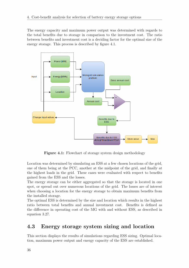
4. Cost-benefit analysis for selection of battery energy storage options

The energy capacity and maximum power output was determined with regards tothe total benefits due to storage in comparison to the investment cost. The ratiobetween benefits and investment cost is a deciding factor for the optimal size of theenergy storage. This process is described by figure 4.1.

Figure 4.1: Flowchart of storage system design methodology

Location was determined by simulating an ESS at a few chosen locations of the grid,one of them being at the PCC, another at the midpoint of the grid, and finally atthe highest loads in the grid. These cases were evaluated with respect to benefitsgained from the ESS and the losses.The energy storage can be either aggregated so that the storage is located in onespot, or spread out over numerous locations of the grid. The losses are of interestwhen choosing a location for the energy storage to obtain maximum benefits fromthe installed storage.The optimal ESS is determined by the size and location which results in the highestratio between total benefits and annual investment cost. Benefits is defined asthe difference in operating cost of the MG with and without ESS, as described inequation 3.27.

4.3 Energy storage system sizing and locationThis section displays the results of simulations regarding ESS sizing. Optimal loca-tion, maximum power output and energy capacity of the ESS are established.

36


4.3.1 Optimal locationTo evaluate the optimal location of the ESS, losses and total benefits of the ESS wascompared for 8 different cases containing both aggregated and distributed energystorage, however, the total ESS size is the same for all cases. These locations chosento be evaluated was the PCC, the two highest loads, L1 and L2, and the bus 07:8.1.Due to the size of the model while using line constraints, it was not possible tosimulate for the whole year. Instead the short-term model was used to simulate thedifferent cases. The size of the ESS during these simulations was chosen to be 6MWh and the results can be seen in table 4.1.Having the ESS at the PCC was found to provide the lowest total cost of energyand losses while having it at L2 proved to be the worst location in both total energycost and losses. There is little difference between having the ESS as a distributedstorage and having it installed as a central ESS at the PCC. This is due to the lowlosses within the system, which is reasonable considering the cables in the grid areover dimensioned. With an increase in battery size the current limits of the cablesmight be exceeded during charging and discharging of the ESS for certain locationsleading to a higher cost since the ESS cannot be operated optimally. At the PCCthis issue will never occur which further implies the optimal location of ESS is atthe PCC.

Table 4.1: Total cost for one day with different ESS locations

Storage Location Benefit [SEK] Loss [kW]PCC 1078.50 40

PCC,07:8.1 1078.40 41L1,L2,PCC,07:8.1 1078.20 43

07:8.1 1078.00 43L1,PCC 1077.40 46L2,PCC 1077.30 48

L1 1072.30 69L2 1071.10 75

4.3.2 Optimal sizeThe total benefits is determined using the EMM, simulating a year of operation.Benefits due to energy storage for different battery capacities is shown in figure 4.2and it is shown that they are increasing with an increased ESS capacity, howeverwith a decreasing rate.The benefits to investment cost ratio is shown in figure 4.3. For the investment tobe economically beneficial the ratio would need exceed to 1. However, as can beseen, the ratio is much lower than 1 meaning that the investment is, from a pureeconomical point of view, not beneficial. There is a decreasing trend in ratio as theESS size increases which means that an increase in installed ESS capacity increasesthe investment cost more than the benefits are increased. The variations seen inthe figure could be due to simulation issues, at some months the GAMS-model was

37


0 2 4 6 8 10 12 14 16 18

Installed Battery Capacity [MWh]

0

0.5

1

1.5

2

2.5

3

3.5

4

4.5

To

tal B

en

efits

[S

EK

]

×105

Figure 4.2: Benefits of battery storage for one year, displayed for different ESSsizes

not able to find an optimal solution due to a high number of non-linearities in themodel formulation. However, the trend is clear despite these variations. This meansthat the optimal ESS size will depend on the island mode operation that is desirablesince simulations do not show a profitable benefit to cost ratio. Instead the optimalsize comes down to what cost the grid operator is willing to pay for the increasedreliability of enabling island mode operation.

4.3.2.1 Sensitivity analysis

A sensitivity analysis is based on changing the parameters used to calculate the CRFfor the investment. With varying lifetime and interest rate the benefit to investmentcost ratio is calculated and shown in figure 4.4. It is shown that with a lower interestrate as well as a longer lifetime of batteries, the investment is considerably better.With dropping prices of energy storage the benefit to cost ratio could be furtherincreased.Figure 4.5 shows the benefit to cost ratio with different prices of batteries, in$/MWh. The lifetime is assumed to 10 years and an interest rate of 3% is used inthis case. It is also shown from figure 4.5 that the benefit to cost ratio is nonlinearfor different prices since the ratio between $200 and $100 is larger than that between$300 and $200. This implies that the lower the prices get the better the investment,thus it could have future economical potential to include ESS in the grid.

38


0 2 4 6 8 10 12 14 16 18


0

0.01

0.02

0.03

0.04

0.05

0.06

0.07

0.08

Be

ne

fit

to C

ost

Ra

tio

Figure 4.3: Benefit to investment cost ratio for different amount of installedstorage.

0 5 10 150

0.05

0.1

0.15Interest rate 3%

0 5 10 150

0.05

0.1

0.15Interest rate 5%

0 2 4 6 8 10 12 14 16 18


0

0.05

0.1

0.15

Be

ne

fit

to C

ost

Ra

tio

Interest rate 7%

n = 10 years

n = 7 years

n = 5 years

Figure 4.4: Benefit to investment cost ratio for different interest rates andexpected lifetimes of storage.

39


0 2 4 6 8 10 12 14 16 18


0

0.05

0.1

0.15

0.2

0.25

0.3

0.35

0.4

0.45

Be

ne

fit

to C

ost

Ra

tio

100 $/kWh

200 $/kWh

300 $/kWh

Figure 4.5: Benefit to investment cost ratio for different battery prices.

40

5Evaluation of Chalmers microgrid

operation scenarios

In this chapter the different cases are described and evaluated. There are four casessimulated, the first one is the base case when the grid is operated with and withoutany storage. The second is island mode to illustrate how the batteries operate duringa disconnection from the main grid. The third one is when an increased renewableenergy generation is present and finally the fourth case is when there is an EV fleetavailable to act as an ESS.

5.1 Case study

The case studies uses the MSP to evaluate how the system will behave and whatbenefits there are by operating the grid as a microgrid during certain circumstances.

5.1.1 Grid connected mode (Base case)

The grid is simulated using the EMM both with and without an ESS and the gainedbenefits are then evaluated. An evaluation of the benefits for running Chalmers’gird as a microgrid in its current state and with an ESS is then made.

5.1.2 Island mode

If there is an outage in the main grid the microgrid can be switched to island mode.To evaluate this, two 1-hour outages where simulated and the grid behavior wasobserved. The ESS together with the local generation is then expected to keep themicrogrid running for the duration of these outages.

5.1.3 Increased renewable generation

With an increased amount of renewable generation the benefit of having a microgridis expected to be higher. In order to verify this, different levels of generation fromsolar PV was simulated to compare the benefits gained with the base case. Theamount of solar PV generation is currently 15.7 kW. Besides from this value, arange from 0 to 3MW are simulated.

41

5. Evaluation of Chalmers microgrid operation scenarios

5.1.4 Vehicle to gridIf there was a significant electric vehicle fleet located at Chalmers, their batteriescould be used as distributed ESS within the microgrid. However, this type of ESSis mobile and might not be available when desired. The vehicles also need to beavailable for driving during all hours of the day so only a portion of their energy canbe used within the microgrid. Assumptions for these simulations are as following:

• Number of vehicles simulated where 25-300, each with a 90 kWh battery in-stalled [33]. Theses vehicles provide a total of 27 MWh of energy when allvehicles are connected.

• The vehicles are available within the grid between hour 8 and 17.• The SOC equations are updated in order to ensure that the vehicles can be

utilized during the day. The new equations specify that the batteries can bevaried between 70 and 100% of their full capacity and they need to be at80% charge at hour 17 which is seen in equation 3.28 and 3.29. The averagecharge is assumed to be 80% when the vehicles arrive in the morning which isdescribed by equation 3.30.

• The net charge gain is assumed to be 0 which means that the vehicles leavewith the same charge as they have when they arrive. It is modeled like thisto simulate the benefits of energy exchange between the vehicles and the grid,not including the cost of charging vehicles to full.

5.2 Case study results

This section handles the case studies conducted in the project. The results of thecase studies are presented and discussed.

5.2.1 Grid connected mode (Base case)The results for different cases where the grid is operated in grid connected mode ispresented in this section. The cases investigated are when no management is doneand when the EMM is implemented, both with and without storage.

• The total annual energy cost for the case where no energy management is doneis 7.0119 MSEK.

• When load curtailment is utilized the total annual energy cost is 7.0062 MSEK,a reduction of 5700 SEK/year.

• For the case when both load curtailment and a 2 MWh ESS is utilized thetotal annual energy cost is 6.9324 MSEK, a reduction of 79500 SEK/year.

The benefits when simulating the microgrid without any storage is small comparedto the total energy cost and thus a poor incentive to implement it. However, theonly load reduction taken into consideration is the ventilation power which couldbe reduced by 20 %, resulting in a total of 100 kW load reduction. If more flexibleloads could be identified the total benefits would be expected to increase. Anotherfactor which affects the benefits is the penalty factor which decides when the loadcurtailment is activated. This factor was set to 240 SEK/MWh, which is 20 %

42


higher than the mean electricity price for 2015. By lowering this factor the annualbenefits would increase by operating the load curtailment more frequently.Power bought from the grid for the cases without EMM and with EMM where a 2MWh ESS is installed for 24-hours (based on data from 17/3-2016) can be seen inFigure 5.1. It can be noted that the ESS has two charging patterns during the day,one in the morning and one in the afternoon, and load curtailment is activated athour 10.

Figure 5.1: Power bought from the grid when EMM is used including ESS andwithout EMM.

5.2.2 Island modeThe minimum sizing of energy storage is determined by its ability to enable themicrogrid to operate in island mode for a certain time. When the microgrid operatesin island mode, the ESS must be able to supply enough power so that the the ESStogether with local generation can supply the demand. Thereby the minimum powerand energy capacity are determined by the maximum load and for how long themicrogrid is to be operated in island mode. The minimum power and energy for theESS are determined by equation 5.1 and 5.2.

PESS,min = Pload,max − PCHP − 0.2Pfan (5.1)

EESS,min = PESS,min · h (5.2)

where h denotes the amount of hours for which the microgrid is operated in islandmode.

43


A fault at the PCC means that no power can be delivered to the microgrid from themain grid. This is simulated by setting the grid power to 0 for hour 4 and 17, thusforcing the ESS to supply the load together with local generation. Figure 5.2 showsthe supply of power within the microgrid for 24 hours with the grid power outageexplained. It can be seen that the ESS is operated to supply the loads when the gridpower is set to zero. It can also be seen from the simulated fault in the afternoonthat the CHP plant is operated in order to supply the loads, since the power fromthe battery is not enough to supply the entire load.

0 5 10 15 20 25

Hour

-5

0

5

10

Active

po

we

r [M

W]

Grid power

ESS power

CHP power

Flexible load

Figure 5.2: Island mode operation with two 1-hour outages

The total energy cost for 24-hours, both in normal conditions and with two 1-houroutages, can be seen in Table 5.1. It can be seen that the cost when island modeis utilized is 224 SEK higher than for normal operations. This cost increase willheavily depend on when the faults occur during the day since both the total loadand the electricity price varies. In this case the disconnection was forced due to afault but it might also be beneficial from an economical point of view to disconnectduring certain hours if the ESS is large enough.

Table 5.1: Total energy cost for 24-hours for normal operation and with two1-hour outages.

Normal operation Two 1-hour faultsCost [SEK] 22400 22624

44


5.2.3 Renewable energy sourcesAn increase in the amount of renewable energy sources within the microgrid wasinvestigated, where the solar PV output power was increased. Simulations usingthe EMM were conducted for values between 0 and 3 MWp from solar PV. Thelifetime of solar cells used in the simulation is 20 years, and for the batteries 5years. An interest rate of 5% is assumed and the cost associated with solar PVinstallation is 1€/Wp [34]. However, the price of solar power is not including anygovernment grants, thus the total investment cost could be decreased further. As forother simulations the battery cost is 300$/MWh. The results are displayed in figure5.3. It is shown that the maximum benefit to cost ratio is obtained with no ESSinstalled, but with increased solar power. It is also shown that for a fixed batterysize, an increase in solar power also increases the benefits gained from ESS. Sincethe solar PV output power is depending on the radiation, the location is of greatimportance. In Sweden solar power is not as beneficial as in other countries withmore sun hours during the year, which could explain why the benefits to cost ratiois not higher than what is shown in figure 5.3.

Installed Solar PV [MWp]

0 0.5 1 1.5 2 2.5 3

Be

ne

fits

to

Co

st

Ra

tio

0

0.05

0.1

0.15

0.2

0.25

No ESS

6 MWh

4 MWh

2 MWh

Figure 5.3: Benefits to investment cost ratio for different ESS sizes, with varyingamount of installed solar power.

5.2.4 Vehicle to gridThe total cost for one year is shown in figure 5.4 assuming the EVs arrive at hour 8and leave at hour 17. The cost is decreasing with an increased amount of EVs, whichis essentially the same as increasing the ESS size. It can be seen that the benefits of

45


having 300 EVs is approximately 100 000 SEK annually, which corresponds to 330SEK per car owner. Such a benefit is a quite poor incentive for car owners to takepart in the V2G system since it will cause the lifetime of their batteries to decrease.The cost reduction is lower than what is accomplished by installing battery storage,and is likely because the EVs are not present during nighttime, therefore the benefitsgained by charging batteries during the low price at night cannot be accomplishedwhen using V2G.The charging pattern is displayed in figure 5.5 where both SOC and power outputfrom the EV fleet is shown. It can be seen that the EVs always have at least 70%charge left during the day so they can be operated if needed. The EVs are alsocharged up to 80 % before they leave so the resulting change of energy during oneday is 0.

Number of EVs

25 50 75 100 125 150 175 200 225 250 275 300

To

tal e

ne

rgy c

ost

for

on

e y

ea

r [S

EK

]

×106

6.9

6.91

6.92

6.93

6.94

6.95

6.96

6.97

6.98

6.99

7

7.01

Figure 5.4: Total cost for one year vs number of EVs.

5.3 Reliability analysisA microgrid should be able to operate independently from the main grid, and there-fore increase its reliability. The amount of local generation and installed ESS willincrease the ability to operate in island mode. Different levels of local generationand ESS sizes where evaluated based on the annual investment cost, annual benefitsand their ability to operate in island mode. The results can be seen in table 5.2.Since solar power is an unreliable resource it might not be available during discon-nection from the main grid, hence the total time in island mode will therefore varyfor the same installed solar capacity. It can be noted that the system can’t be op-

46


Hour

0 5 10 15 20 25

Po

we

r o

utp

ut

[MW

]

-1

-0.5

0

0.5

1

Hour

0 5 10 15 20 25

SO

C

0.6

0.7

0.8

0.9

1

Figure 5.5: Output power PEV and SOC during one day of operation.

erated in island mode without any ESS for the solar levels tested. This is due tothe power levels the peak load requires to operate. There is a possibility to operateparts of the microgrid with only solar installed at these levels, however, this has notbeen investigated further.The enhancement of reliability within the system comes from the battery storage,and can be associated with a cost which comes from the annual investment cost andthe annual benefit. By subtracting the benefits from the annual investment cost, thetotal cost per hour of island mode can be calculated. For battery storage of 6 MWhthis cost is calculated to 1.684 MSEK/year for one hour of island mode capability.

Table 5.2: Comparison of different investment costs, annual revenues and islandmode operation times for different ESS and solar PV sizes

Installed batterycapacity [MWh]

Installed solarpower [MWp]

Annual investmentcost [MSEK]

Annual benefit[MSEK]

Island modeoperation [h]

0 0 0 0 00 3 2.17 0.432 02 1.5 1.70 0.287 0.33-0.52 3 2.79 0.490 0.33-0.664 1.5 2.33 0.345 0.66-0.84 3 3.41 0.560 0.66-1.06 0 1.86 0.176 16 3 4.03 0.590 1-1.33

The different sizes for the ESS investigated were 2, 4 and 6 MWh. Paired with 3MWp solar PV installed, the island mode operation time can be seen in Figure 5.6.

47


There are two contributions to the total island mode time: first the reliable timewhich comes from batteries and secondly the unreliable time from solar PVs. Thesetimes are based on a worst case scenario meaning that the load is at its peak value.Other means of improving island mode operation time could be to increase reliablelocal generation, such as CHP. However, no investigation on this has been made.

Installed ESS size [MWh]

2 4 6

Ho

urs

of

isla

nd

mo

de

op

era

tio

n

0

0.2

0.4

0.6

0.8

1

1.2

1.4

Time from ESS

Time from solar

Figure 5.6: Island mode operation time for different ESS sizes with 3 MWp solarPV installed

The total energy cost can be reduced by introducing battery storage in the microgrid,or by investing in increasing the amount of solar PV. Figure 5.7 compares the totalenergy cost for one year. The base case is compared to different ESS sizes, withEVs and also for one case with 6 MWh of battery storage and 3 MWp of solarpower. The total energy cost is reduced when more energy storage is installed,however the maximum cost reduction is obtained by including both battery storageand increasing the amount of solar PV. Including EVs as a mean of storage withinthe grid reduces the cost by 2.49%. The total energy cost can be reduced by asmuch as 8.43% when including both battery storage and increasing the amount ofsolar PV.

48


Base case 300 EVs 2,4 and 6MWh 6MWh and 3MWp75

80

85

90

95

100

To

tal co

st

[%]

EVs

ESS and solar PV

ESS

Figure 5.7: Total energy cost compared to base case for different configurationsincluding battery storage, solar power and EVs.

49


50

6Conclusions and Future work

6.1 Conclusions∗

This thesis was focused on three different objectives. Firstly, a database of the griddata and load profiles for each bus in the Chalmers microgrid was developed. A loadprofile for 24 hours was extracted from measurements and then extended to cover anentire year. The second objective was to use the database to create an EMM in orderto simulate the grid operating as a microgrid. This model involves local generation,variable loads, fixed loads, grid data and ESS. It was realized using GAMS and themodels validity was then confirmed by using PSS/E. The final objective was to usethe model in order to observe the benefits by operating the grid as a microgrid.This was accomplished by several case studies where the grid was operated underdifferent circumstances.

• Base case operation when the grid was run as a microgrid was compared to thecurrent operating state. Here, no ESS was available so the benefits originatefrom scheduling the local generation and the flexible loads. It is shown thatthe total cost can be lowered by 5700 SEK.

• Part of operating a grid as a microgrid is the ability to run it in island mode.This was implemented and tested for two one-hour outages where the grid wasoperated independently for one hour. The simulation results shows that witha proper ESS size the grid can withstand a disconnection to the main grid forone hour.

• More renewable energy resources, in the form of solar PV, were implementedin the grid and the benefits were evaluated for different ESS sizes. It was foundthat the optimal solution was to only invest in solar since the cost of ESS isvery high compared to the benefits. However, by only investing in solar PVthe ability to operate in island mode is lost due to the unreliable nature ofsolar power. Therefore, an investment in both solar and ESS is more suitablefor this microgrid.

• By using an EV fleet in place of an ESS, the total energy cost can be reducedby approximately 100 000 SEK annually for 300 vehicles. This eliminates theneed to invest in additional ESS but the grid infrastructure needs to be furtherdeveloped to realize this. There is also the matter of battery degradation whenusing EVs in a microgrid and the owners must therefore be compensated for

∗The results from this thesis has been summarized in the paper: "Cost-benefit analysis of batterystorage investment for microgrid of Chalmers university campus using OPF framework" shown inappendix A.2

51

6. Conclusions and Future work

this to be a viable option.The study shows that there is value in operating the grid as a microgrid and withadditional local generation and ESS the total energy cost for the system can belowered by 8.43% while being able to operate in island mode for a minimum of 1hour.

6.2 Future Work• Linearization of the EMM - The power flow equations and other constraints are

highly non-linear which causes high simulation time. By linearizing constraintsthe medium-term model could be used for energy storage location studies andalso reduce the simulation time overall.

• Energy storage alternatives - Further investigation of cheaper alternatives toenergy storage and comparisons of investment in storage and local generationcould be conducted.

• Load control in MG - Investigation of flexible load possibilities could also beinteresting since the battery size could be reduced if only critical loads were tobe supplied during island mode operation. To gain a more accurate model ofwhen the ventilation power can act as a flexible load, measurements regardingtemperature and carbon dioxide in the buildings need to be incorporated in themodel. The Ventilation can only be down regulated if the levels of temperatureand carbon dioxide are within acceptable limits.

• Taxes and grid tariff - Including taxes, peak power cost and fixed grid costsin the model would give a more accurate representation of the energy cost.This could have an impact on how beneficial the ESS would be and how it isutilized.

• Utilization of CHP - The usage of the heat distribution from the CHP plantcould also be investigated to reduce the cost of operating the plant. As itlooks now, all the heat is assumed to be wasted and the cost for electricityproduction is therefore high. Also ramp-up and ramp-down constraints for theCHP plant needs to be incorporated for a more accurate model.

• Load profile resolution - To actually be able to operate Chalmers’ grid as amicrogrid, the load profile needs to be on a shorter time scale. This needs tobe measured on each individual bus, and these kind of measurements does notexist today.

52

References

[1] G. Pepermans et al., "Distributed generation: definition, benefits and issues."Energy policy, vol. 33, no. 6, pp.787-798, April 2005.

[2] A.A Salam et al., "Technical challenges on microgrids," in ARPN Journal ofEngineering and Applied Sciences, vol.3, no. 6, pp. 64-69, December 2008.

[3] Q. Fu et al., "The Role of Energy Storage in a Microgrid Concept: Examiningthe opportunities and promise of microgrids.," in IEEE Electrification Maga-zine, vol. 1, no. 2, pp. 21-29, Dec. 2013.

[4] R. H. Lasseter and P. Paigi, "Microgrid: a conceptual solution," 2004 IEEE 35thAnnual Power Electronics Specialists Conference (IEEE Cat. No.04CH37551),2004, pp. 4285-4290 Vol.6.

[5] B. S. Hartono et al., "Review of microgrid technology," QiR (Quality in Re-search), 2013 International Conference on, Yogyakarta, 2013, pp. 127-132.

[6] J. Marecki "Combined heat & power generating systems," IET; 1988, (Vol.3 pp.1-2).

[7] X.Tan, Q.Li,H.Wang, "Advances and trends of energy storage technology inMicrogrid," International Journal of Electrical Power & Energy Systems, Vol.44, no 1, pp. 179-191, January 2013.

[8] A. Poullikkas, "A comparative overview of large-scale battery systems for elec-tricity storage," Renewable and Sustainable Energy Reviews, vol. 27, pp.778-788, November 2013.

[9] R.E. Chiez, J.F. Whitacre, "Comparative techno-economic analysis of hybridmicro-grid systems utilizing different battery types," Energy Conversion andManagement, Vol. 112, pp. 435-444, March 2016.

[10] B. Nykvist, M- Nilsson, "Rapidly falling costs of battery packs for electric ve-hicles," Nature Climate Change, Vol 5, no 4, pp. 329-332, 2015.

[11] W. Kempton, J. Tomić, "Vehicle-to-grid power fundamentals: Calculating ca-pacity and net revenue," Journal of power sources, Vol 144, no 1, pp. 268-279,2005.

[12] W. Kempton, J. Tomić, "Vehicle-to-grid power implementation: From stabi-lizing the grid to supporting large-scale renewable energy," Journal of powersources, Vol 144, no 1, pp. 280-294, 2005.

[13] B. Bolund, H. Bernhoff, M. Leijon, "Flywheel energy and power storage sys-tems." Renewable and Sustainable Energy Reviews, vol 11, no 2, pp. 235-258,February 2007.

[14] R. Sebastián, RP. Alzola, "Flywheel energy storage systems: Review and simu-lation for an isolated wind power system," Renewable and Sustainable EnergyReviews, Vol 16, no 9, pp. 6803-6813, December 2012.

53

References

[15] I. Hadjipaschalis, A. Poullikkas, V. Efthimiou, "Overview of current and futureenergy storage technologies for electric power applications," Renewable and sus-tainable energy reviews, vol 13, no 6, pp. 1513-1522, September 2009.

[16] D. Steen., "Modelling of Demand Response in Distribution Systems." Ph.D.dissertation, Dept of Energy and Environment, Chalmers University of Tech-nology, Gothenburg, Sweden, 2014.

[17] A. Oudalov, R. Cherkaoui and A. Beguin, "Sizing and Optimal Operation ofBattery Energy Storage System for Peak Shaving Application," Power Tech,2007 IEEE Lausanne, Lausanne, 2007, pp. 621-625.

[18] Su, Wencong, and Jianhui Wang. "Energy management systems in microgridoperations," The Electricity Journal, vol. 25, no 8, pp.45-60, October 2012.

[19] S. X. Chen et al., "Sizing of Energy Storage for Microgrids," in IEEE Transac-tions on Smart Grid, vol. 3, no. 1, pp. 142-151, March 2012.

[20] C. Chen et al., "Optimal Allocation and Economic Analysis of Energy StorageSystem in Microgrids," in IEEE Transactions on Power Electronics, vol. 26, no.10, pp. 2762-2773, Oct. 2011.

[21] N.W.A Lidula, A.D Rajapakse, "Microgrids research: A review of experimentalmicrogrids and test systems," Renewable and Sustainable Energy Reviews,Vol15, no 1, pp. 186-202, 2011.

[22] R.Lasseter, A.Khalsa. (2016, May 13). CERTS Microgrid Test Bed [Online].Availible: https://certs.lbl.gov/initiatives/certs-microgrid-test-bed

[23] G. Turner, J. P. Kelley, C. L. Storm, D. A. Wetz and W. J. Lee, "Design andActive Control of a Microgrid Testbed," in IEEE Transactions on Smart Grid,vol. 6, no. 1, pp. 73-81, Jan. 2015.

[24] R. M. González, T. A. J. van Goch, M. F. Aslam, A. Blanch and P. F. Ribeiro,"Microgrid design considerations for a smart-energy university campus," IEEEPES Innovative Smart Grid Technologies, Europe, Istanbul, 2014, pp. 1-6.

[25] M. Meiqin, S. Shujuan and L. Chang, "Economic analysis of the microgridwith multi-energy and electric vehicles," 8th International Conference on PowerElectronics - ECCE Asia, Jeju, 2011, pp. 2067-2072.

[26] E. Hossain, E. Kabalci, R. Bayindir , R. Perez, "Microgrid testbeds around theworld: State of art," Energy Conversion and Management, vol 86, pp.132-153,October 2014.

[27] Elsayed et al., "DC microgrids and distribution systems: An overview." in Elec-tric Power Systems Research, vol.119, pp. 407-419, February 2015.

[28] X. Liu, P. Wang and P. C. Loh, "A Hybrid AC/DC Microgrid and Its Coordina-tion Control," in IEEE Transactions on Smart Grid, vol. 2, no. 2, pp. 278-286,June 2011.

[29] Justo, Jackson John, et al. "AC-microgrids versus DC-microgrids with dis-tributed energy resources: A review," Renewable and Sustainable Energy Re-views, vol. 24, pp.387-405, August 2013.

[30] Nordpool web page (2016, May 27) [Online].Available: http://www.nordpoolspot.com/

[31] International Electrotechnical Commission. Photovoltaic devices—Part 3: mea-surement principles for terrestrial photovoltaic (PV) solar devices with referencespectral irradiance data. IEC 60904–3 ed2, 2008

54

References

[32] GAMS web page (2016, September 16) [Online].Available: http://www.gams.com/

[33] Model S Specifications (2016, Aug 31) [Online].Avalible: https://www.tesla.com/support/model-s-specifications?redirect=no

[34] Mayer JN, Simon P, Philipps NS, Schlegl T, Senkpiel C. "Current and futurecost of photovoltaics," Long-term Scenarios for Market Development, SystemPrices and LCOE of Utility-Scale PV Systems (Fraunhofer ISE, Study on behalfof Agora Energiewende, Freiburg, 2015). 2015 Mar.

55

References

56

AAppendix 1

A.1 GAMS Code

*Defining setsset i buses /1*41/;alias(i,j);set h hour;set d(h) daytime;set Head2 Line data table headings / Re, Xe, Ch /;

*Parameter definitions$parameter P_load(i,h) load at bus i and hour h;$$parameter Q_load(i,h) img load at bus i and hour h;$$parameter Elprice(h) electricity cost at hour h;$$parameter Pmax(i) max Pgen at bus i /13 inf, 16 1/;$$parameter Qmax(i) max Qgen at bus i /13 inf, 16 0.3/;$$parameter Pemax(i);$$parameter Ilim(i,j);$$parameter Pfan(i,h);$$parameter Psolar(i,h);$

*Scalar definitionsscalar Emax;scalar phi /3.141592654 /;scalar Sbase base in MVA /1/;scalar CostCHP SEK per MW /600/;scalar chr efficiency of energy storage /0.95/;scalar dis efficiency of energy storage /0.95/;

*Input data loaded from MATLAB code\$GDXIN Z:\.win\Desktop\GAMS\1year_model.gdx\$LOAD h=Hour\$LOAD d=Daytime\$LOAD Elprice=Elspot\$LOAD P_load=Load_real\$LOAD Q_load=Load_img

I

A. Appendix 1

\$LOAD Pemax=Pemax\$LOAD Emax=E_max\$LOAD Ilim=I_lim\$LOAD Pfan=Pfan\$LOAD Psolar=Psolar\$GDXIN

display Elprice,P_load,Q_load,Pemax,Emax;

*Line data for the grid in p.u, used to form an admittance matrixTable LineData(i,j,Head2)

Re Xe Ch1.2 0.0000000 0.0208110 0.000001.3 0.0000853 0.0000580 0.001001.5 0.0000798 0.0000535 0.000973.4 0.0000000 0.0737500 0.000005.6 0.0000635 0.0000308 0.000485.12 0.0003120 0.0002113 0.003805.41 0.0001306 0.0000580 0.000856.7 0.0000000 0.0580000 0.000008.9 0.0000000 0.0725000 0.000008.17 0.0001252 0.0000844 0.0015010.11 0.0000000 0.0602500 0.0000010.41 0.0001868 0.0000825 0.0012012.13 0.0000145 0.0000010 0.0001712.16 0.0000172 0.0000118 0.0002112.17 0.0000227 0.0000154 0.0002812.18 0.0000281 0.0000190 0.0003513.14 0.0004762 0.0003229 0.0058014.15 0.0000000 0.0132430 0.0000016.19 0.0000281 0.0000190 0.0003517.31 0.0003746 0.0002540 0.0046017.33 0.0000907 0.0000617 0.0011018.22 0.0000000 0.0440000 0.0000018.23 0.0002549 0.0001732 0.0031018.35 0.0004535 0.0003075 0.0055019.20 0.0000000 0.0223170 0.0000023.24 0.0000000 0.1067500 0.0000023.25 0.0003401 0.0002304 0.0042025.26 0.0000000 0.0600000 0.0000025.27 0.0001868 0.0001270 0.0023027.28 0.0000000 0.0612500 0.0000029.30 0.0000000 0.0725000 0.0000029.35 0.0004653 0.0003156 0.0057031.32 0.0000000 0.0360000 0.00000

II

A. Appendix 1

33.34 0.0000000 0.0393750 0.0000035.36 0.0000000 0.0361930 0.0000035.38 0.0000118 0.0000082 0.0001438.39 0.0000363 0.0000109 0.0001239.40 0.0000000 0.0208000 0.0000041.21 0.0000000 0.0334360 0.00000;

*Admittance matrixParameter Z(i,j), GG(i,j), BB(i,j), YCL(i);Parameter G(i,j), B(i,j), Y(i,j), ZI(i,j), Theta(i,j);

LineData(j,i,"Re")$(LineData(i,j,"Re") gt 0.00) = LineData(i,j,"Re");LineData(j,i,"Xe")$(LineData(i,j,"Xe") gt 0.00) = LineData(i,j,"Xe");LineData(j,i,"Ch")$(LineData(i,j,"Ch") gt 0.00) = LineData(i,j,"Ch");

Z(i,j) = (LineData(i,j,"Re"))**2 + (LineData(i,j,"Xe"))**2 ;GG(i,j)$(Z(i,j) ne 0.00) = LineData(i,j,"Re")/z(i,j) ;

BB(i,j)$(Z(i,j) ne 0.00) = -LineData(i,j,"Xe")/Z(i,j);BB(j,i)$(Z(i,j) ne 0.00) = -LineData(i,j,"Xe")/Z(i,j);

YCL(i) = sum(j, LineData(i,j,"Ch"));

B(i,i) = sum(j, BB(i,j)) + YCL(i);G(i,i) = sum(j, GG(i,j));G(i,j)$(ord(i) ne ord(j)) = -GG(i,j);B(i,j)$(ord(i) ne ord(j)) = -BB(i,j);

Y(i,j) = sqrt(G(i,j)*G(i,j) + B(i,j)*B(i,j));

ZI(i,j)$(G(i,j) ne 0.00) = abs(B(i,j))/abs(G(i,j));

Theta(i,j) = arctan(ZI(i,j));Theta(i,j)$((B(i,j) eq 0) and (G(i,j) gt 0)) = 0.0;Theta(i,j)$((B(i,j) eq 0) and (G(i,j) lt 0)) = -0.5*phi;Theta(i,j)$((B(i,j) gt 0) and (G(i,j) gt 0)) = Theta(i,j);Theta(i,j)$((B(i,j) lt 0) and (G(i,j) gt 0)) = 2*phi - Theta(i,j);Theta(i,j)$((B(i,j) gt 0) and (G(i,j) lt 0)) = phi - Theta(i,j);Theta(i,j)$((B(i,j) lt 0) and (G(i,j) lt 0)) = phi + Theta(i,j);Theta(i,j)$((B(i,j) gt 0) and (G(i,j) eq 0)) = 0.5*phi;Theta(i,j)$((B(i,j) lt 0) and (G(i,j) eq 0)) = -0.5*phi;Theta(i,j)$((B(i,j) eq 0) and (G(i,j) eq 0)) = 0.0 ;

Display Y, Theta

III

A. Appendix 1

*Variable definitionsVARIABLESQ(i,h) Reactive power generation at bus i and hour hP(i,h) Active power generation at bus i and hour hV(i,h) Voltage at bus i and hour hCost Total system costLoss Total system transmission lossesDelta(i,h) Voltage angle in radiansSOC(i,h) State of charge at bus iPec(i,h) Charge power from ESS at bus i and hour hPed(i,h) Discharge power from ESS at bus i and hour hRevenue Total revenue of storageReI(i,j,h) Real part of current between bus i and j at hour hImI(i,j,h) Imaginary part of current between bus i and j at hour hPflex(i,h) Amount of flexible load at bus i and hour hQbatt(i,h) Reactive power from batteries at bus i and hour hIabs(i,j,h) Absolute current;

*Equation definitionsEQUATIONSCostFn Total system generation cost in $Equn1(i,h) Real power load flow equationEqun2(i,h) Reactive power load flow equationSOC1(i,h) SOC equationSOC2(i,h) SOC equationTotgen(h) Total power generatedTotrev Total revenueRI(i,j,h) Real part of current between busesII(i,j,h) Imaginary part of current between busesFlexeq(i,h) Equation to limit load curtailmentChargeEq(i,h) Charge equationItot(i,j,h) Absolute currentIli Current limitation equationIli2 Current limitation equation;

*Constraints on variablesV.up(i,h) = 1.05;V.lo(i,h) = 0.95;

Q.up(i,h) = Qmax(i);

IV

A. Appendix 1

P.up(i,h) = Pmax(i);

Pflex.lo(i,h) = 0;Pflex.up(i,h) = 0;Pflex.up(i,d)= 0.2*Pfan(i,d);

Qbatt.up(i,h) = 0.3*Pemax(i);Qbatt.lo(i,h) = -0.3*Pemax(i);

SOC.up(i,h) = 1;SOC.lo(i,h+1)$(Pmax(’13’) gt 0) = 6/Emax;SOC.lo(i,h+1)$(Pmax(’13’) eq 0) = 0;SOC.fx(i,’1’)$(Pemax(i) ne 0) = 6/Emax;

Pec.up(i,h) = Pemax(i);Pec.lo(i,h) = 0;Ped.up(i,h) = Pemax(i);Ped.lo(i,h) = 0;

*Equation limiting to load curtailmentFlexeq(i,h)$(ord(h) ne card(h)).. Pflex(i,h)*Pflex(i,h+1)*10000000 =e= 0;

*Load flow equationsEqun1(i,h).. P(i,h) - P_load(i,h) + dis*Ped(i,h) - Pec(i,h) + Psolar(i,h) +Pflex(i,h) =e= Sum(j, Y(i,j)*V(i,h)*V(j,h)*Cos(theta(i,j) + Delta(j,h) -Delta(i,h)));Equn2(i,h).. Q(i,h) - Q_load(i,h) + Qbatt(i,h) + tan(arccos(0.98))*Pflex(i,h)=e= -Sum(j, Y(i,j)*V(i,h)*V(j,h)*Sin(theta(i,j) + Delta(j,h) - Delta(i,h)));

*SOC equationsSOC1(i,h)$(ord(h) ne 1).. SOC(i,h) =e= SOC(i,h-1)+chr*Pec(i,h-1)/(Emax)-Ped(i,h-1)/(Emax);SOC2(i,h)$(ord(h) eq card(h)).. Pe(i,h) =e= (SOC(i,h)-SOC.lo(i,h))*Emax;

*Charge equationChareEq(i,h).. Pec(i,h)*Ped(i,h) =e= 0;

*Calculation of revenueTotRev.. Revenue =e= sum((i,h),Pe(i,h)*Elprice(h))*Sbase;

*Equations for line constraints

V

A. Appendix 1

RI(i,j,h).. ReI(i,j,h) =e=V(j,h)*Y(i,j)*COS(Theta(i,j)+Delta(j,h)) -V(i,h)*Y(i,j)*COS(Theta(i,j)+Delta(i,h)) +V(i,h)*LineData(i,j,"ch")*SIN(Delta(i,h));

II(i,j,h).. ImI(i,j,h) =e= V(j,h)*Y(i,j)*SIN(Theta(i,j)+Delta(j,h))- V(i,h)*Y(i,j)*SIN(Theta(i,j)+Delta(i,h)) +V(i,h)*LineData(i,j,"ch")*COS(Delta(i,h));

Itot(i,j,h).. Iabs(i,j,h) =e= sqrt(power(ReI(i,j,h),2) + power(ImI(i,j,h),2));

Ili(i,j,h).. Iabs(i,j,h) =l= Ilim(i,j);Ili2(i,j,h).. Iabs(i,j,h) =g= -Ilim(i,j);

*Objective function - Total costCostFn.. Cost =e= (sum(h,P(’13’,h)*Elprice(h)+P(’16’,h)*CostCHP)+sum((i,h),Pflex(i,h)*240))*Sbase;

*Model formulation describing which equations are included in the modelmodel OPF /Equn1Equn2CostFnChargeEqSOC1SOC2TotrevFlexeqRIIIItotIliIli2/;

*Solve statementsolve OPF using NLP minimizing Cost;

*Output data to MATLABexecute_unload ’results’,Cost,SOC,Pec,Ped,Revenue;

VI

Cost-benefit analysis of battery storage investmentfor microgrid of Chalmers university campus using

OPF frameworkMartin Goransson, Niklas Larsson and Le Anh Tuan

Department of Energy and EnvironmentChalmers University of Technology

Gothenburg, SwedenEmail: [email protected]

Abstract—This paper presents a cost-benefit approach forevaluation of battery energy storage (BES) options to be installedin the electrical distribution grid of Chalmers University from themicrogrid perspective. The evaluation is based on a multi-periodac optimal power flow (OPF) model applied for microgrid, whichis referred to as the µ-OPF, with the objective function being thetotal grid operation cost. The model is developed for the real 12kV grid of Chalmers. The µ-OPF is used as the calculation toolfor the cost-benefit analysis where the benefit-to-cost ratios (BCR)of battery options in the grid in a year over the annualized costof battery are evaluated for various options of battery placementsin the grid. The BCRs demonstrate the cost-effectiveness ofthe battery in microgrid operation. Battery options consideredinclude both distributed option and a centralized option. Ithas been found that the optimal location of battery storage atChalmers grid is at the point of connection to upstream gridof Gothenburg Energy distribution system. The study resultsshow that the benefit gained from using battery storage increaseswith the size of battery, and the size with the highest BCR wasfound to be 2 MWh when considering the grid-connected modeof operation. The optimal size when the grid is in island modeis however dependent on island mode capability.

Index Terms—Microgrid, Battery energy storage (BES), Flexi-ble demand, Solar PV, Cost-benefit analysis, University Campus

NOMENCLATURE

SetsH Total number of hours in the simulation time-

horizonK Total number of buses in the microgridIndicesh Hourd Hour during day-timei, j Indices for busesV ariablesTC Total grid operation costP gridh Power from the main gridPCHPh Power from the combined heat and power

(CHP) plant

The work presented in this paper is partly funded by Energy Area ofAdvance of Chalmers University of Technology.

∆P loadi,h Active load curtailment

∆Qloadi,h Reactive load curtailment

P geni,h Active power generation at bus i and hour hQgen

i,h Reactive power generation at bus i and hour hV Voltage magnitudeI Current magnitudeSOC State of charge of batteryP eci,h Active power to battery storage during chargingP edi,h Active power from battery storage during dis-

chargingQBES

i,h Reactive power from battery storageEi,h Stored energy at bus i for hour hParametersErated

i Installed battery energy storage at bus iBi,j Imaginary element of the admittance matrixGi,j Real element of the admittance matrixCgrid

h Cost to buy power from main gridGCHP Unit generation cost of the CHP plantPF Penalty factor for load curtailmentP fani,d Total fan load for bus i and hour dP loadi,h Active power load at bus i and hour hQload

i,h Reactive power load at bus i and hour hV mini Minimum voltage magnitudeV maxi Maximum voltage magnitudeI limi,j Maximum current limit on line i-jeff chr Charging efficiency of battery storageeffdis Discharging efficiency of battery storage

I. INTRODUCTION

The increasing penetration of small-scale distributed energyresources (DERs), including wind power, solar photovoltaics(PV), micro combined heat and power (CHP) units, etc. andthe electric vehicles (EVs) in the distribution system put aquite challenging task to the distribution system operator tocontrol and operate the system in a reliable manner. Themicrogrid concept has been introduced to partially addressthis challenge [1]. A microgrid is generally defined as alocal cluster with a clear geographical boundary within a

A. Appendix 1

A.2 Summarized paper

VII

distribution system, which can coordinate the operation ofDERs and energy storage to supply the local load demandin an economic and reliable manner [2], [3]. Microgrids offerboth technical and economic benefits to the distribution systemoperators. With many microgrids developed, the control ofDERs in the distribution system can be passed on to the localcontrol in the microgrids. Microgrids can be operating in grid-connected as well as off-grid (island) modes. Microgrids thushelp to utilize the DERs to their fullest extent. Customerswithin microgrid would expect to have more reliable electricitysupply service, thanks to the capability to operate in bothmodes. The distribution system will benefit from microgridsince it will minimize the peak power demand in the distribu-tion system, reduce the need for power transmission, and thusincrease the overall efficiency.

Microgrid development has recently been taking place atseveral university campus environment, including Eindhovenuniversity of technology [4], university of Genoa [5], [6]. Thecommon goals for these university campuses’ microgrid are toimprove the economic performance of the grid and to reducethe use of fossil-based generation. Chalmers University ofTechnology has identified microgrid as one of its strategicresearch areas. One of the projects in microgrid which hasrecently received funding from EU Urban Innovative Actionprogram [9] would focus on transformaing electrical gridof Chalmers University of Technology into an intelligentmicrogrid which can be used as microgrid test bed. This testbed will support investigations of methods and strategies fordesign, control, protection, operation of microgrids. The aimis also to demonstrate a concept of fossil-free energy district inmodern urban context. As a first step in this project, an initialinvestigation of microgrid design has to be perform. One ofthe tasks in this step is to identify the optimal placement ofbattery energy storage (BES) within the microgrid.

Energy storage is an important component in a microgrid,which can be used for demand response, storing excess energyand support island mode operation. Cost-benefit analysis is oneof common approaches to evaluate the cost-effectiveness of theinvestment which can be applied for the case of battery energystorage in microgrid. A number of work has been presented inthis topic. The most relevant work was found in [7] in whicha method for choosing the optimal size was developed basedon a cost-benefit analysis for both islanded and grid connectedmicrogrids. The total benefits are calculated for values betweena chosen minimum and maximum energy storage size in orderto obtain the most beneficial size. However, constraints onphysical electrical grid were not considered. Also, the modelused is only for 24-hour period. This present paper proposed acost-benefit analysis which is based on a multi-period optimalpower flow model built on the one developed in [8] withdetailed ac load flow constraints and the model is applied forthe whole year (8760 hours) to evaluate the benefit of differentcandidates of battery storage. The main contributions of thispresent paper can be summarized below:• Development of the grid model: Data for Chalmers’ inter-

nal electrical distribution grid was not readily available

for grid simulation. This data has been acquired throughdifferent methods and used for simulating the grid. Also,collection and evaluation of whole-year demand profilesat building levels and solar generation data of Chalmerscampus has been made.

• Development of µ-OPF model: The µ-OPF model forChalmers microgrid was developed with the objectivefunction being the total grid operation cost (i.e., cost ofenergy imported which is considered to be dependent ofthe spot price electricity plus the cost of own productionfrom the CHP plant). Technical constraints in the modelsinclude power flow constraints, battery state of chargelimits, as well as other constraints of flexible demands inthe grid. A simulation platform was created using GAMS[10] as the modeling and optimization tool and MATLAB[11] for data handling and automation.

• Proposed cost-benefit analysis for BES: The paper hasproposed to use cost-benefit analysis approach basedon µ-OPF model for 1-year simulation study period toevaluate the battery energy storage candidates which canreflect the variations in load and solar energy as well asweather conditions over the whole year.

II. DEVELOPMENT CHALMERS’ DISTRIBUTION GRIDMODEL AND DATABASE

A. Grid data

The internal electrical grid at Chalmers is used to distributepower to the campus and consists of 22 buses where 17 areload buses and can be seen in Fig. 1. Akademiska Hus [12]provided data of cables and transformers, from which a loadflow model of Chalmers grid has been implemented.

B. Load profile and flexible demand

Demand profiles for each bus (i.e., building) in the grid havebeen extracted based on current (I) measurements by the ABBMicro-SCADA system and energy demand for each buildingprovided by Akademiska Hus [12]. The current (I) measure-ments are extracted and stored for every 10-minute intervalwith a backlog for only 24 hours. Therefore, a scaling factorbased on the energy consumption was used to approximatethe demand profile for one year. A load profile was measuredfor a day in March 2016, with peak load of 5.5 MW at hour14. The total power demand at Chalmers varies between 2.5and 7.0 MW and the annual energy consumption is 32000MWh. The main loads in the campus include e.g., lighting,computers, ventilation, and electric machines in laboratories.There are a number of EVs currently in use in the campuswhich represents distributed BES.

Flexible demand due to adjustments in the ventilation powerwithin building in Chalmers grid is possible to a certain extent.The ventilation power is a total of 500 kW spread out overthe campus and can be reduced temporarily by 20%. This loadreduction can only occur during the day-time, between whenthe ventilation is operating at maximum capacity and only forone hour at a time so that the working environment remainscomfortable. Activation of the load curtailment is assumed

A. Appendix 1

VIII

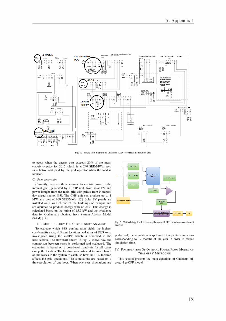
Fig. 1. Single line diagram of Chalmers 12kV electrical distribution grid

to occur when the energy cost exceeds 20% of the meanelectricity price for 2015 which is at 240 SEK/MWh, seenas a fictive cost paid by the grid operator when the load isreduced.

C. Own generation

Currently there are three sources for electric power in theinternal grid, generated by a CHP unit, from solar PV andpower bought from the main grid with prices from Nordpoolday ahead market [13]. The CHP unit can produce up to 1MW at a cost of 600 SEK/MWh [12]. Solar PV panels areinstalled on a wall of one of the buildings on campus andare assumed to produce energy with no cost. This energy iscalculated based on the rating of 15.7 kW and the irradiancedata for Gothenburg obtained from System Advisor Model(SAM) [14].

III. METHODOLOGY FOR COST-BENEFIT ANALYSIS

To evaluate which BES configuration yields the highestcost-benefits ratio, different locations and sizes of BES wereinvestigated using the µ-OPF, which is described in thenext section. The flowchart shown in Fig. 2 shows how thecomparison between cases is performed and evaluated. Theevaluation is based on a cost-benefit analysis for all casesexcept the location. The location was instead determined basedon the losses in the system to establish how the BES locationaffects the grid operations. The simulations are based on atime-resolution of one hour. When one year simulations are

Fig. 2. Methodology for determining the optimal BES based on a cost-benefitanalysis

performed, the simulation is split into 12 separate simulationscorresponding to 12 months of the year in order to reducesimulation time.

IV. FORMULATION OF OPTIMAL POWER FLOW MODEL OFCHALMERS’ MICROGRID

This section presents the main equations of Chalmers mi-crogrid µ-OPF model.

A. Appendix 1

IX

• Objective function: The objective of the model is tominimize the total operation cost of the system includingthe cost of energy import, cost of own production as wellas the cost of demand control.

TC =∑

h∈H

∑

i∈KPCHPh CCHP

+ P gridh Cgrid

h + PF∆P loadi,h (1)

• Power flow equations with battery storage and flexibledemand:

P geni,h − P load

i,h + P eci,h − effdis ∗ P ed

i,h + ∆P loadi,d

=∑

j∈K|Vi||Vj |(Gi,j cos θi,j +Bi,j sin θi,j) (2)

Qgeni,h −Qload

i,h +QBESi,h + ∆Qload

i,d

=∑

j∈K|Vi||Vj |(Gi,j cos θi,j −Bi,j sin θi,j) (3)

The voltage magnitudes, Vi, and current magnitudes, Ii,j ,are limited according to (4) and (5).

V mini ≤ Vi ≤ V max

i (4)

|Ii,j | ≤ I limi,j (5)

where, V mini and V max

i are the minimum and maximumvoltage levels and I limi,j is the maximum allowed currentbetween bus i and j.

• Flexible demand constraints:Installed ventilation power is currently 500 kW and canbe reduced by 20 % when desired according to (6).

∆P loadi,d ≤ 0.2 ∗ P fan

i,d (6)

The frequency at which the load curtailment occurs islimited to every other hour as seen in (7).

∆P loadi,d ∗∆P load

i,d+1 = 0 (7)

• Battery energy storage constraints:The BES is modeled as either a charging or dischargingpower. Monitoring is done by observing the state ofcharge (SOC), which is defined by (8) and limited by(9).

SOCi,h =Ei,h

Emaxi

(8)

0 ≤ SOCi,h ≤ 1 (9)

Variations of the SOC over the simulation period iscalculated as seen in (10). Since the model uses a onehour data resolution the power utilized by the BES canbe compared to the energy capacity of the BES.

SOCi,h = SOCi,h−1+eff chr ∗ P ec

i,h−1Erated

i

−P edi,h−1

Eratedi

(10)

The µ-OPF model is of non-linear programming type. It hasbeen implemented in GAMS environment [10] and solvedusing MINOS solver [15].

V. SUMMARY OF STUDY RESULTS

This section presents preliminary results of the paper includ-ing optimal location for BES and total benefits for differentsizes of BES for a 1-year period. In the full version of thepaper, the following results will be discussed and presented:

• Optimal configuration of BES, including location andsize, based on a cost-benefit analysis and island modecapabilities.

• Energy scheduling during island mode operation• A more accurate load profile including different load

within each building to establish more flexible loads• Sensitivity analysis of benefits of storage with respect to

changes in capacity of local generation, solar PVs, andprices of battery storage.

Different aspects of the BES were varied to achieve anoptimal configuration with regards to the total energy costand island mode capabilities. Four different locations forconnection of battery storage were investigated for both anaggregated and a distributed BES, yielding a total of eightcases which where evaluated regarding the line losses. Theconsidered connection point for BES are shown by the circlesin Fig. 1. Those include point of common coupling (PCC) (i.e.,the main grid connection point), the two most heavily loadedbuses (L1 and L2) to enable the highest loads to be efficientlysupplied. The introduction of BES at the high load buseswould further increase the load when the batteries are charged,however the batteries are charged during low price hours whichcorrelates to the hours with lower demand. Finally, bus 07:8.1was also investigated. These simulations have been carried outfor a time span of 24 hours with a total installed BES size of6 MWh.

TABLE IBES LOCATION COMPARISON

Location Loss [kW]

PCC 40

PCC, 07:8.1 41

PCC, 07:8.1, L1, L2 43

07:8.1 43

PCC, L1 46

PCC, L2 48

L1 69

L2 75

A. Appendix 1

X

0 2 4 6 8 10 12 14 16 18


0

0.5

1

1.5

2

2.5

3

3.5

4

4.5

Tota

l B

enefits

[S

EK

]

×105

Fig. 3. Total benefits for different BES capacities

As shown in Table I, the configuration which yields thelowest losses is to place the entire BES at the PCC which isused for all further simulations. The worst cases are to havethe BES entirely at L1 or L2, due to the higher loading on thelines during charging and discharging of the BES.

When the microgrid is operated in grid-connect mode, theBES is used for demand response by charging when the energyprice is low and discharging when the price is high. This willreduce the total energy cost which is a benefit to the microgridoperator (Akademiska Hus in this case). The total benefit fordifferent BES sizes has been shown in Fig. 3. It can be seenfrom the figure that total benefits increase as the BES capacityincreases, however at a decreasing rate. This means that itmight not be beneficial to invest in more storage than necessaryfor the desired island mode operation time.

Operation in island mode is possible when an BES isinstalled with enough capacity to supply the demand, togetherwith local generation, for the duration of an outage due tofault in the upstream grid. During that time, the BES issupplying the demand together with the local generation andbeing recharged during the succeeding hours to be ready foranother possible outage.

VI. CONCLUSIONS

This section presents preliminary conclusions from thework. More concrete conclusions will be made in the fullversion of the paper.

In this paper, a multi-period optimal power flow model formicrogrid has been developed using the real data from theelectrical distribution grid of Chalmers university campus. Themodel has been used in the pre-design phase of microgrid forChalmers to evaluate cost-effectiveness of the battery storageoptions. It has been found that the operation of Chalmers as amicrogrid as scheduled by the µ-OPF model for the operationof battery storage, demand responses as well as own generationwould reduce the total operation cost as well as the total energyloss in the grid. The optimal battery storage option has been

suggested based on the highest benefit-to-cost ratio obtainedover the whole year. It was shown in the study that the benefitfrom battery has not outweighed its investment cost, giventhe high market price of the battery storage at the present.It can be expected that the price of the battery storage willgo further down in the future which will improve the cost-effectiveness of the battery. In this study, the battery storagehas only been considered for supplying energy in Chalmersmicrogrid, consideration of other use of battery storage, suchas grid support services to the distribution system and powerbalancing services could further enhance the battery cost-effectiveness. This is however the subject of further study.

ACKNOWLEDGMENT

The authors would like to thank Per Loveryd, Richard Blockand their colleagues at Akademiska Hus for providing the dataof Chalmers’ grid. Thanks are also extended to David Steenat Chalmers for his discussions and support with the work.

REFERENCES

[1] Hatziargyriou, N.; Asano, H.; Iravani, R.; Marnay, C., ”Microgrids,”in IEEE Power and Energy Magazine, vol.5, no.4, pp.78-94, July-Aug.2007.

[2] Parhizi, S.; Lotfi, H.; Khodaei, A.; Bahramirad, S., ”State of the Artin Research on Microgrids: A Review,” in Access, IEEE , vol.3, no.,pp.890-925, 2015

[3] Eklas Hossain, Ersan Kabalci, Ramazan Bayindir, Ronald Perez, Mi-crogrid testbeds around the world: State of art, Energy Conversion andManagement, Volume 86, October 2014, Pages 132-153, ISSN 0196-8904,

[4] R. Morales Gonzalez, T. A. J. van Goch, M. F. Aslam, A. Blanch,and P. F. Ribeiro, ”Microgrid design considerations for a smart-energyuniversity campus,” IEEE PES Innovative Smart Grid Technologies,Europe, Oct. 2014.

[5] S. Bracco, F. Delfino, F. Pampararo, M. Robba, and M. Rossi, ”Theuniversity of Genoa smart polygeneration microgrid test-bed facility:The overall system, the technologies and the research challenges,”Renewable and Sustainable Energy Reviews, vol. 18, pp. 442459, Feb.2013.

[6] S. Bracco, F. Delfino, F. Pampararo, M. Robba, and M. Rossi, ”Eco-nomic and environmental performances quantification of the universityof Genoa smart Polygeneration Microgrid,” 2012 IEEE InternationalEnergy Conference and Exhibition (ENERGYCON), Sep. 2012.

[7] S. X. Chen, H. B. Gooi, and M. Q. Wang, ”Sizing of energy storagefor Microgrids,” IEEE Transactions on Smart Grid, vol. 3, no. 1, pp.142151, Mar. 2012.

[8] W. Feng, L. A. Tuan, L. B. Tjernberg, A. Mannikoff and A. Bergman,”A New Approach for Benefit Evaluation of Multiterminal VSCHVDCUsing A Proposed Mixed AC/DC Optimal Power Flow,” in IEEETransactions on Power Delivery, vol. 29, no. 1, pp. 432-443, Feb. 2014.

[9] Urban Innovative Actions web page (2016) [Online].Available: http://www.uia-initiative.eu/en

[10] General Algebraic Modeling System (GAMS) Version 23.9.5. Washing-ton, DC: GAMS Development Corporation., 2012.

[11] MATLAB, Version R2014b. Natick, Massachusetts: The MathWorksInc., 2014.

[12] Akademiska Hus web page (2016) [Online].Available: http://www.akademiskahus.se/en/

[13] Nordpool web page (2016, May 27) [Online].Available: http://www.nordpoolspot.com/

[14] System Advisor Model (SAM) Version 2016.3.14 Washington, DC:National Renewable Energy Laboratory., 2016.

[15] MINOS solver manual, [Online].Available: https://www.gams.com/

A. Appendix 1

XI

A. Appendix 1

A.3 Load Profile

Table A.1: Load profile for each hour of a day, 17/3-2016

Hour Load [kW]1 3519.52 3521.83 3534.64 3546.75 3579.36 3672.97 4206.08 4679.39 5059.410 5325.911 5367.712 5413.913 5454.814 5472.915 5461.416 5293.817 4884.018 4545.519 4215.720 3974.821 3817.522 3718.323 3610.524 3534.2

XII

A. Appendix 1

Figure A.1: Load data for all buses in Chalmers grid 17/3-2016

XIII

A. Appendix 1

Figure A.2: Load data for all buses in Chalmers grid 17/3-2016

XIV

development of an energy management model for chalmers...

Documents