Development of Components to

Realize Control of an Electrostatic

Actuator

TOMMY TRAM

Master of Science Thesis

Stockholm, Sweden 2011

Development of Components to Realize

Control of an Electrostatic Actuator

Tommy Tram

Master of Science Thesis MMK 2011:48 MDA 417

KTH Industrial Engineering and Management

Machine Design

SE-100 44 STOCKHOLM

Master of Science Thesis MMK 2011:48 MDA 417

Development of Components to Realize Control

of an Electrostatic Actuator

Tommy Tram

Approved

2011-06-17

Examiner

Mats Hanson

Supervisor

Bengt Eriksson

Commissioner

The University of Tokyo

Contact person

Akio Yamamoto

Abstract

At the University of Tokyo, Higuchi and Yamamoto lab, there is an electrostatic actuator that is

capable of moving sheet-like semi-conductive material by electrostatic force.

This thesis presents the development of a set of basic components to realize control of the

electrostatic actuator. The position of the object that is moved by the actuator is tracked by using

a camera and image processing algorithms.

Two approaches are presented, one by using OpenCV to track a specific color and one by using

ARtoolkit to track a specific marker. The ARtoolkit method is chosen because it is less sensitive

to noise and is more stable than the OpenCV method.

A PIC micro-controller with an interface on a PC is implemented to allow a computer program

to control the electrostatic actuator. Using only the PIC controller and a computer program, the

actuator could operate at about 86 mm/s as its maximum speed. The combination of the PIC

controller and the position detection program module will allow various motions of the

electrostatic motor.

Examensarbete MMK 2011:48 MDA 417

Utveckling av komponenter för att realisera

reglering av ett elektrostatiskt ställdon

Tommy Tram

Godkänt

2011-06-17

Examinator

Mats Hanson

Handledare

Bengt Eriksson

Uppdragsgivare

The University of Tokyo

Kontaktperson

Akio Yamamoto

Sammanfattning

I Higuchi och Yamamoto laboratoriet på Tokyo Universitetet har det utvecklats en elektrostatiskt

ställdon som kan förflytta pappersliknande halvledande material med hjälp av elektrostatiska

fält.

I denna rapport presenteras utvecklingen av ett antal grundlägande komponenter för att realisera

reglering av ett elektrostatiskt ställdon. Genom att använda bildbehandlig samt en kamera kan

man fastställa positionen av objektet som styrs av det elektrostatiska ställdonet.

Två alternativa bildbehandlings algoritmer studeras, en som använder sig av OpenCV för att

filtrera ut en specifik färg och en som använder sig av ARtoolkit för att hitta ett specifikt

mönster. ARtoolkit metoden valdes på grund av att den är mindre kännslig till störningar och

stabilare än OpenCV metoden.

Ett grafiskt gränsnitt samt en PIC mikrokontroller används för att styra det elektrostatiska

ställdonet från en dator, med hjälp av USB kommunikation. Den elektrostatiska ställdonet

förflyttar objeket med en tophastighet på 86 mm/s. Kombinationen av posisionerings systemet

och styrelektroniken möjligör reglering av det elektrostatiska ställdonet.

Acknowledgements

I would like to thank Associate Professor Yamamoto Akio for guiding me through the

electrostatic experiments and Professor Mats Hanson for making it possible to continue the thesis

at The Royal Institute of Technology after returning from Japan.

I would also like to thank Mr. Nils Emil Söderbäck for helping me integrate the GUI with

OpenGL and ARtoolkit, and PhD. Masayuki Hara for the color detection algorithm.

I am also grateful to the finical support of the Interdisciplinary Global Mechanical Engineering

(IGM) Project under the Industrialized Countries Instrument Education Cooperation Program

(ICIECP) from the European Community (Agreement number ICI - 2008 - JAP – 146129).

Tommy Tram

Stockholm, May 2011

Abbreviations

ARtoolkit Augmented Reality Toolkit

GLUT OpenGL Utility Toolkit

OpenCV Open Source Computer Vision Library

OpenGL Open Graphics Library

PC Personal Computer

PIC Peripheral Interface Controller

USB Universal Serial Bus

Table of Contents

1. Introduction ................................................................................................................... 1

1.1. Background ................................................................................................................. 1

1.2. Problem ....................................................................................................................... 1

1.3. Purpose ....................................................................................................................... 2

1.4. Delimitation ................................................................................................................ 2

1.5. Method ........................................................................................................................ 2

1.6. Reference Literature ................................................................................................... 2

2. Tools to Develop Components......................................................................................... 3

2.1. Design Concept of the Entire System......................................................................... 3

2.2. Electrostatic Actuator ................................................................................................. 3

2.3. Electrical Components ................................................................................................ 5

2.4. Program Library ......................................................................................................... 5

2.4.1 OpenGL ................................................................................................................ 5

2.4.2 OpenCV ................................................................................................................ 5

2.4.3 ARtoolkit .............................................................................................................. 5

3. Development of Components .......................................................................................... 6

3.1. Drive Circuit for the Electrostatic Actuator............................................................... 6

3.2. Control Signal Logic from the PIC ............................................................................. 7

3.3. Graphical User Interface ............................................................................................ 8

3.4. Computer Animation .................................................................................................. 8

3.5. Position Tracking of the Slider ................................................................................... 9

3.5.1. Color Tracking using OpenCV............................................................................. 9

3.5.2. Marker Detection Using ARtoolkit ................................................................... 10

4. Evaluation of the Designed Components ...................................................................... 11

4.1. Animation and Slider Tracking Integration ............................................................ 11

4.1.1. Collision Detection with ARtoolkit .................................................................... 11

4.1.2. Comparing with OpenCV .................................................................................. 12

4.2. Experiment Setup for Testing of Drive Circuit ........................................................ 12

4.3. Setting up Drive Circuit, PIC and PC ...................................................................... 13

4.4. Driving the Slider ..................................................................................................... 14

4.5. Reversing the Motion of the Slider ........................................................................... 15

4.6. Limitations of the System ........................................................................................ 16

4.7. Maximum Speed ....................................................................................................... 17

4.8. Recover Slider Motion ............................................................................................... 19

5. Conclusions, Discussion and Recommendation for Future Work .................................. 21

5.1. Conclusion ................................................................................................................. 21

5.2. Discussion ................................................................................................................. 21

5.3. Recommendation for Future Work ........................................................................... 22

6. References .................................................................................................................... 23

1

1. Introduction

1.1. Background

An electrostatic motor has been developed at The University of Tokyo, Higuchi and Yamamoto

lab, which can transport light semi-conductive material, such as plastic sheet. The object that is

transported on an electrostatic actuator is referred to as a slider. The actuator is made out of

transparent material, as shown in Figure 1, and is driven by applying a high-voltage three-phase

signal. Although this technology has existed from 1990 [1], it does not yet have an effective

application.

Figure 1. Transparent Electrostatic Actuator and Slider

1.2. Problem

Recently, an application has been proposed for this electrostatic actuator, which is a new type of

human-computer interface [2]. In the proposed application, a transparent electrostatic actuator is

set on a surface of a computer screen. Using the electrostatic actuation, a PC program can move

sheet-like objects on the screen, which can also be moved by a user. A user and a PC program

can share the same physical object, through which they can interact each other in a very different

way from the conventional human-computer interactions.

To realize such an application, several components need to be developed. The electrostatic

actuator today has no sensors that can track the position of an object on the actuator. For the new

human-computer interaction, a sensor needs to detect the position of the object on the actuator.

Another important component is a drive circuit. In previous research, the actuator was mostly

driven by using a signal generator that can generate predefined signal patterns. To facilitate the

human-computer interaction, a drive circuit that allows control of the actuator from a PC

program is needed.

2

1.3. Purpose

The goal of this thesis is to provide components for the above-mentioned application. The

components include a visual tracking program that allows tracking the motion of the objects on

the electrostatic actuator. For this purpose a simple web-camera is used as an input device.

Another component to be developed is a drive circuit that has an interface with Windows-based

computer to allow control of the actuator from a PC program. Some other components which

will be required to realize the human-computer interaction are also included in this thesis.

1.4. Delimitation

This thesis presents the development of the components needed to control the electrostatic

motor. The components that re developed can be used to control an electrostatic actuator. The

evaluation of the actuators performance will be based on the system setup explained in chapter

4.2. The PC program will use functions from program libraries to design the components.

1.5. Method

The development process consists of planning, literature study, technology evaluation, concept

generation, concept evaluation, analyze and validation. Several conference proceedings about the

electrostatic technology were studied to understand the driving of the actuator. Studies about

OpenGL and other libraries were also done to design possible solutions for this application.

1.6. Reference Literature

The conference paper by Yamamoto, A., Yoshioka, H. and Higuchi, T. (2006) A 2-DOF

Electrostatic Sheet Conveyer Using Wire Mesh for Desktop Automation [2] was mainly studied

to understand the technology behind the electrostatic actuator. Because the technology is

relatively new, other conference papers were also studied and can be found at the end of this

report.

The book by Shreiner, D. and Woo, M. OpenGL programming guide: the official guide to

learning OpenGL [3] was studied to learn how to make computer animations and also to explore

the animation possibilities.

For computer vision, the book by Bradski, G., and Kaehler, A. Learning OpenCV: Computer

vision with the OpenCV library [4] was studied to understand the fundamentals behind the image

processing.

3

2. Tools to Develop Components

This chapter explains the tools and methods needed to develop components to realize the control

of an electrostatic motor.

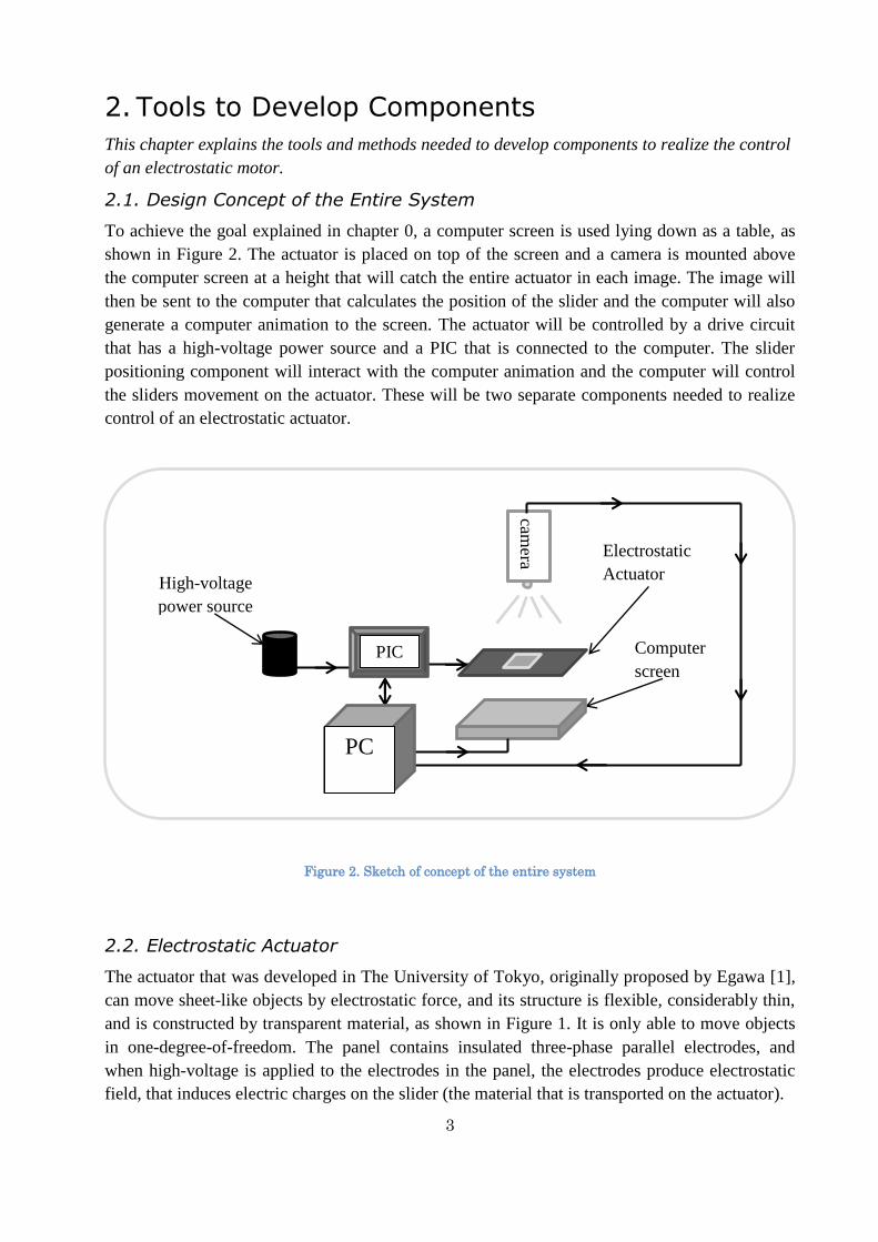
2.1. Design Concept of the Entire System

To achieve the goal explained in chapter 0, a computer screen is used lying down as a table, as

shown in Figure 2. The actuator is placed on top of the screen and a camera is mounted above

the computer screen at a height that will catch the entire actuator in each image. The image will

then be sent to the computer that calculates the position of the slider and the computer will also

generate a computer animation to the screen. The actuator will be controlled by a drive circuit

that has a high-voltage power source and a PIC that is connected to the computer. The slider

positioning component will interact with the computer animation and the computer will control

the sliders movement on the actuator. These will be two separate components needed to realize

control of an electrostatic actuator.

Figure 2. Sketch of concept of the entire system

2.2. Electrostatic Actuator

The actuator that was developed in The University of Tokyo, originally proposed by Egawa [1],

can move sheet-like objects by electrostatic force, and its structure is flexible, considerably thin,

and is constructed by transparent material, as shown in Figure 1. It is only able to move objects

in one-degree-of-freedom. The panel contains insulated three-phase parallel electrodes, and

when high-voltage is applied to the electrodes in the panel, the electrodes produce electrostatic

field, that induces electric charges on the slider (the material that is transported on the actuator).

camera

Computer

screen

High-voltage

power source

Electrostatic

Actuator

PC

PIC

4

The driving procedure is done by applying three different voltages to the three electrodes

positive voltage, negative voltage and ground [1]. This set of charges is referred to as [+,-,0], as

displayed in Figure 3. As an initial step the actuator needs to keep (1) charge setting for a short

while so the slider can generate a mirrored charge pattern (to the actuators charge pattern) in the

surface of the slider (2). To then drive the slider, the charges on the electrode shift places from

[+, -, 0] to [0, +, -] (3). The different charges between actuator and slider will cause the slider to

attract toward the later pattern (4) in this case to the right. Repeating pattern (2)-(4) will cause

the slider to move. The actuator is controlled by applying a three-phase high-voltage waveform

signal like in Figure 4.

Figure 3. Principle of actuation [1]

Figure 4. Voltage waveforms for driving [1]

5

2.3. Electrical Components

A PIC will be used to control the actuator with commands given from a PC. The PIC used in this

project is named PIC18F4550 and is a 40-pin microcontroller with integrated USB 2.0 module.

The PIC itself is powered by the voltage supplied by the computer via USB but the high-voltage

needed to control the actuator is supplied by two DC-DC converters that amplify 12V into 600V,

this driving voltage is also discussed in chapter 5.1. Nine AVQ258 relays are used to switch

between the positive and negative high-voltage sources, to generate the necessary signal shown

in Figure 4.

2.4. Program Library

The program language C++ is used to design the PC program, because there are several useful

libraries to develop this application. Libraries are sets of functions defined so that any developer

can select and use them to create their own applications. Different libraries contain different sets

of functions and are developed for different applications. Three libraries are studied in this

thesis; OpenGL that can be used to generate a computer animation, OpenCV and ARToolKit that

can both be used to localize the position of the slider.

2.4.1 OpenGL

OpenGL is a library for writing applications that produce 2D and 3D computer animations.

There are over 250 different functions that can be used to draw the complex three dimensional

structures [3]. There is an additional library called GLUT that uses a combination of OpenGL

functions to handle computer windows and commonly used animations, e.g., it is possible in

GLUT to draw a sphere with just one function, while in OpenGL, the user has to define all the

circles adding up to one sphere. This can be used to show the interaction between a PC program

and the physical slider.

2.4.2 OpenCV

The OpenCV library consists of programming functions, mainly aiming at real time image

processing [4]. This library can handle the camera and the image taken from it, e.g., OpenCV can

be used in face recognition or motion tracking. The functions are easily combined with a camera

and are compatible with OpenGL. It can be used to process the images taken from the camera to

track the sliders position.

2.4.3 ARtoolkit

The final library is a high level library used to build augmented realities applications, these

applications involve overlaying of virtual imagery on the real world [5]. The virtual images are

usually displayed based on a markers position in the real world. ARtoolkit has many tracking

and features i.e., it can track position and orientation of a marker, an example of a marker is

displayed in Figure 11. ARtoolkit can be used for detecting and localize the object moved by the

actuator by placing a marker on top of the object.

6

3. Development of Components

This chapter explains how the components for this project are developed.

3.1. Drive Circuit for the Electrostatic Actuator

To generate the control signal explained in chapter 2.2, two DC-DC converters are used to

generate the high voltage sources [+,-,0]. One is used to generate the positive (+) signal, the

other to generate the negative (–) signal and their ground signal are connected together to

generate a common ground. Relays are used to switch between the three different voltage

sources and to generate the phase pattern in chapter 2.2. Each phase has three relays and each

relay is connected to a signal source, a total of nine relays. The relays are then controlled by a

PIC controller that uses three output pins total to manage the relays. Every control pin is

connected to three relays and each connected to different power sources, i.e., the PIC control pin

RD7 is connected to the three relays K1-K3, as shown in Figure 5. This will work as a controlled

switch between the power source HV and the electrode PH. Where the HV is the high voltage

signals generated from the amplifiers and PH is the connection to the electrodes. This means that

each control pin will release 3 relay switches and generate one type of signal to each electrode,

e.g., when the RD7 pin gives a low signal (0V), the relay K1 will connect the high-voltage

positive source to electrode-phase A, while the relay K2 connects the ground signal to electrode-

phase B and finally the relay K3 will connect electrode-phase C with the negative high-voltage

source.

Figure 5. Driving Circuit with PIC and relays

Input high-votage signals

Control pins

Relays K1-K3

7

3.2. Control Signal Logic from the PIC

The computer together with a PIC controls the actuators movement by sending control bits from

the computer to the PIC, via USB connection. The PIC controls the relays to generate the three-

phase signal explained in chapter 3.1. The start block Figure 6 represents when power is supplied

to the PIC and from there the PIC does the necessary initiations to establish a communication.

The “communication task” handles the communication buffers on the PIC, i.e., it sends the data

stored in the send buffer and reads the data in the receive buffer. Depending on the information

in the receive buffer, the “I/O process” will execute the necessary settings to move the actuator.

Figure 6. PIC flow chart from powering the PIC to shutting it down

Figure 7 displays the “I/O process”, from Figure 6, in more detail. It starts by checking if the

USB connection is correctly configured and if the data are received from the PC, before making

any changes to the actuator. Depending on what command code is received from the buffer, the

PIC will switch the relays, from chapter 3.1, to make the actuator act as commanded.

Figure 7. I/O Process block in more detail

8

3.3. Graphical User Interface

A GUI is developed to control the PIC by USB communication. The PC program sends

predefined command bits to the PIC to control the systems actions and the PIC receives these

commands and acts according to them, this can be viewed in chapter 3.2. The GUI can make the

PIC change the acceleration, speed and direction of the actuator, each action sends its own

command byte. It can also receive the current values from the PIC and display them, as shown in

Figure 8. This GUI is used in chapter 0 to evaluate the performance of the actuator and the drive

circuit.

Figure 8. The graphical user interface used in the experiments

3.4. Computer Animation

A simple animation program is written, with the OpenGL library, to demonstrate interactions

between physical object on the actuator and computer animation. The program starts by initiating

the window’s size and position using GLUT. The animation is similar to a planet orbiting around

the sun, with a smaller sphere rotating round the sphere in the middle. The whole animation will

constantly move back and forth in the horizontal direction, when it hits a certain x-coordinate it

will enter a function which reveres the direction, as shown in Figure 9. This function can later be

triggered depending on the position of the slider. The x-coordinates have a default value at the

end of the arrows.

Figure 9. OpenGL animation

Movement direction

9

3.5. Position Tracking of the Slider

Two ways of tracking the position of an object on the electrostatic actuator are studied. Both

methods use a camera mounted above the actuator. The first method is to put a strong color on

the object and use the images to filter out the central position of that color. The other method is

to use a predefined marker, a picture which the camera can recognize. A simple USB web-

camera, QuickCam Pro 4000 from Logitech, is used to capture the images of the slider to the

computer.

3.5.1.Color Tracking using OpenCV

The first method starts by capturing an image using the camera. From OpenCV, the function

“cvSplit” is used to split the image into three separate images [4]. Each image contain red, green

or blue channel. The image with the red channel is then made in to a binary image with a defined

threshold, as shown in Figure 10. Then the blue and green images are made into an inverted

binary image, with the same function “cvThreshold”. The next step is to use the function

“cvAnd” and match the three binary images to sort out the color red. The last image in Figure 10

shows the binary red image.

Figure 10. Color filtering process

Also in OpenCV there is a function, “cvMoments”, that calculates the moment of each pixel in

the image, moment is the calculated sum of the distance from the upper right corner to an

existing binary white pixel.

10

This is then used to calculate the center of the binary red image by using equation (1). Where

Mp,q are values given by the function “cvMoments”, xp is the x-coordinate of the pixel and xg is

the x-coordinate for the pixel placed in the center of the white area, the same thing is then done

for the y-coordinate. The first image in Figure 10 shows a yellow dot at the center part of the red

object.

3.5.2.Marker Detection Using ARtoolkit

The marker is a predefined figure or a sign in a black square, as displayed in Figure 11. What

ARtoolkit does is very similar to the previous method. It takes a picture with the camera and

generates a binary image, and in that image ARtoolkit finds and locates the 3D coordinate of the

black square so it can match the symbol inside the figure with the predefined one [5]. With this

ARtoolkit can evaluate the orientation of the marker. The pixel coordinates are then transferred

to matrix coordinates that can be used in OpenGL as a set point for where to draw the animation.

Figure 11. ARtoolkit marker, where the triangle is the predefined figure

xMM g0010

MMy

g00

01

n

i

qp

qp yxM yxI1

,,

n

i

yxIM1

00,

n

ixM yxI

1

1

10,

xMM

g

00

10

(1)

11

4. Evaluation of the Designed Components

This chapter evaluates the components from chapter 3. The animation is integrated with the

slider positioning algorithms and experiments are done on the drive circuit integrated with the

PC program to evaluate the performance of the system. It will check if the voltage signals given

from the drive circuit explained in chapter 3.1 are correct and the performance of the whole

system, in terms of speed and stability.

4.1. Animation and Slider Tracking Integration

Both methods to track the sliders positions are tested with an animation that will be generated by

using GLUT and OpenGL functions, explained in chapter 3.4. Slider tracking and computer

animation will be combined to create a system that allows a computer animation to interact with

a sliders position. Collision detection is done first by using ARtoolkit and OpenGL, where

ARtoolkit locates the slider by mapping out the marker coordinates while the OpenGL keeps

track of the animations coordinates.

4.1.1.Collision Detection with ARtoolkit

With the sliders coordinates form the ARtoolkit, the camera constantly updates the position of

the slider. The sliders position is then compared to the position on the animation, if the slider is

within the range of the animations moving area in the y-plane. Step 1 in Figure 12 marks the red

area as a non-collision zone. This means that if the marker is inside the red area it cannot collide

with the animation, the white arrows shows the movement direction of the objects. If the slider is

within the collision range in the y axis, then the program will compare the x-coordinate of the

marker and the animation. If the marker and the animation are in close range of each other as

displayed in step 3. The animation will change direction, as shown in step 4, and a signal will be

given to the GUI indicating a collision between animation and the physical sheet.

Figure 12. Collision step by step

2.

3. 4.

1.

12

4.1.2. Comparing with OpenCV

The color tracking method gives the coordinates in form of pixel coordinates. This will make the

integration with OpenGL animation a bit more difficult. Also the color filtering method is very

dependent on light. If there is too much light the positioning will be inaccurate but with too little

light the coordinates will be very noisy. The ARtoolkit-method is also dependent on light, but

not as much as the color tracking. Because the ARtoolkit method matches a more complex shape

and form the coordinates are more stable than the color tracking method. ARtoolkit is easy to use

but very difficult to modify. This application is simple enough to just use the marker detection

functions without modifying. The coordinates that are given are compatible with the coordinates

used to define the location of the animation.

4.2. Experiment Setup for Testing of Drive Circuit

These experiments are done with the drive circuit explained in chapter 3.1, the PIC commands

from chapter 3.2 and a GUI from chapter 3.3. The displacement laser, LM10 ANR1215, has a

±50 mm measuring range measuring object for the displacement laser. An oscilloscope, that can

read 4 inputs simultaneously, is used that corresponds to a -5/+5V signal. A plastic object is

placed on top of the slider as to reflect the light from the laser displacement sensor. Probes are

used to measure voltage and current on the drive circuit.

Figure 13. Experiment setup to evaluate the performance of the drive circuit together with the GUI

Displacement Laser

Slider

Measuring Object

Drive circuit

13

4.3. Setting up Drive Circuit, PIC and PC

After connecting the PC and PIC together, three probes are connected from the oscilloscope to

the output voltages from the drive circuit, marked as PH_A, PH_B and PH_C in Figure 5. The

results are displayed in Figure 14 where each plot corresponds to the voltage supplied to an

electrode on the actuator. This experiment is done without the actuator connected.

Figure 14. Output signal from drive circuit

The three graphs in Figure 14 show that the drive circuit, PIC and PC successfully generated the

voltage pattern explained chapter 2.2.

14

4.4. Driving the Slider

The setup for the next measurements are done with two probes measuring the high-voltage the

same way as in previous experiment, but the third probe is measuring the current in PH_A, from

Figure 5. and the fourth input to the oscilloscope is from the displacement laser. The actuator is

connected for this experiment, the measurement values are shown in Figure 15. In this

experiment, the “current for Phase A” graph illustrates the current for one electrode input on the

actuator and the “Displacement Laser” graph shows the displacement of the slider, measured

with the displacement laser.

How many pitches the slider transports each phase change can be calculated with (2), where y1 is

the position of the slider before moving one pitch and y2 is the position after moving step. One

pitch p is the distance between the electrodes and d is the number of pitches. This is interesting

to monitor the limitations of the pitch distance.

Figure 15. Actuator voltage input, current and displacement

As shown in Figure 15, the “Phase A” and “Phase B” graph, the input signal is much slower

from a -600V to 0V. The difference came from the capacitance of the electrostatic actuator.

Since the actuator is a capacitance load, it increases the time constant of the charging and

discharging of voltages. But because the charges from the other electrodes are dominant, the

slider can still move. The “Current for Phase A” graph shows the current applied to the actuator,

where a current displacement occurs due to phase changes.

(2)

15

4.5. Reversing the Motion of the Slider

To study the behavior of the actuator when reversing direction of the slider while moving, the

actuator is driven at a constant speed and from the GUI inverts the phase shift to change

direction. The setup is the same as previous chapter and the measurements are shown in Figure

16.

Figure 16. Inverting the phase while in movement

No unexpected changes were discovered in this experiment and can therefore say that it is safe

for the system to invert the phase while moving the slider.

16

4.6. Limitations of the System

The limitations of drive circuit can be observed by accelerating the phase shift, for the control

signals given by the PIC, at the fastest frequency possible. For this experiment the second probe

is changed to measure the control PIN on the PIC, it measures the control signal given from RD7

and are shown in “Output PIC RD7”. The measurements are shown in Figure 17.

Figure 17. Moving with acceleration

“Displacement Laser” graph shows that the slider stopped moving after accelerating. “Phase A”

shows that the actuator doesn’t get the high-voltage needed to drive although “Output PIC RD7”

graph shows the control signal is given from the PIC. This means the relays on the drive circuit

are too slow for the frequency changes received from the PIC control signal.

17

4.7. Maximum Speed

The next experiment determines what the highest possible speed is for the slider, with this setup.

The speed of the slider is decided by the frequency of the phase changes. Because the actuator

needs to start at a low frequency, the slider is driven with acceleration up to different values of

maximum frequencies. The value that can maintain the slider in motion after the acceleration can

be determined as the maximum speed.

Several experiments are done with different frequencies on the control signal, from the PIC.

Figure 18 shows the measurements from the actuator at the frequency where the slider does not

move after the acceleration. The frequency can be calculated in both Figure 18 and Figure 19 by

inverting the time it takes to get a new signal by using equation (3) on the “Output High

Voltage” graph, where x1 is the time from first signal and x2 is the time from the second signal.

Figure 18. Slider stopped moving after acceleration

Figure 18 show that the slider lost contact and conductivity due to the high frequency. This

experiment is repeated until a stable frequency is found.

(3)

18

After running the actuator at the same frequency five times without the slider stopping, the

measurement is recorded in Figure 19. It shows that the actuator still moving after the

acceleration at the fastest frequency possible. Observation showed the slider still moving even

outside of the laser measurement area.

Figure 19. Slider moving at maximum speed

This experiment is able to drive the slider at a maximum speed without losing connection to the

actuator. The constant speed can be determined by calculating the derivative in the fourth graph

in Figure 19, while the slider is keeping constant speed. This makes it possible to calculate the

speed with (4) at the time 2.5 and 3 seconds.

[

]

(4)

19

4.8. Recover Slider Motion

The next experiment will try to recover moment of the slider after it is lost due to too high

frequency phase shifts. When the slider loses motion it will cause the charges on the slider to

lose it pattern, the charge pattern has to be restored to regain motion. This is done by charging

the sliders charges at low frequency, this experiment will run the slider at a speed that makes the

slider lose motion. The actuator will then, from the GUI, restart the acceleration at from a lower

frequency and accelerate up to a higher speed, the measurements are shown in.

Figure 20. Restarting the Acceleration to Recover Motion on the Slider

The slider couldn’t recover motion just by restarting the acceleration, as shown in Figure 20. The

motion can be recovered, by turning the control signal off for a second and afterwards restart the

acceleration. It takes a couple of seconds for the actuator to charge the slider back into motion.

20

21

5. Conclusions, Discussion and Recommendation

for Future Work

This chapter summarizes the projects results and conclusions, discussions about the project and

recommendations for future work.

5.1. Conclusion

Chapter 4.1 showed that ARtoolkit was more stable than the color tracking method. With the

color tracking method the coordinate was easily disrupted if a hand was captured in the image,

and also very sensitive to light. The ARtoolkit library was much more difficult and complicated

to apply, but once the installation and initiations was complete, the functions that are supplied by

that library were very useful.

The precision of the drive circuit could be evaluated from chapter 4.6. The “Displacement Laser”

graph in Figure 17 shows that the slider has stopped moving around the “2 seconds” mark, while

the PIC is still giving output signals. This was because the slider moved too fast and the slider

lost the electrostatic charge. The “Phase A” and “Current for RD7” graph shows that the input to

the actuator is at zero. The relays were not able to switch on before the phase changed again.

That lead to that no current or voltage could pass through to the actuator. The conclusion that the

drive circuit has an upper frequency limit due to the relays was be made.

The maximum speed that the slider could traveled by this actuator could be calculated with

equation (4) at the time interval 2.5 seconds and 3 seconds, from Figure 19. The maximum speed

measured up to 84.9 mm/s. The frequency in Figure 18 and Figure 19 is the fastest frequency the

relay can switch between. This is the frequency limit for the system to be able to move the slider.

From the “Output High Voltage” graph in Figure 19 and equation (3) a frequency of 55 Hz was

calculated for the input signal while the PIC had 83 Hz output.

Two major components have been developed to realize control of an electrostatic actuator. The

collision detection program can be used as a sensor for the slider, to keep track of the sliders

position anywhere within the image captured by the camera. The second component is the drive

circuit combined with the PIC and GUI allows free control of the actuator from a computer. The

position of the slider can be controlled by using these two components.

5.2. Discussion

The driving voltage at 600V is limited by breakdown, in theory we could apply up to

approximately 1000V. If higher voltage is applied, then there is a change of electrical discharge

in the air. This actuator was specially fabricated from a company that no longer makes it, that’s

why 600V was a safe driving voltage was applied so that it would not risk breakdown of the

actuator.

Many planned experiments could not be done due to an earthquake accident in Japan that caused

me to return to Sweden. The equipment stayed in The University of Tokyo but the thesis

finalized at The Royal Institute of Technology in Stockholm. Experiments on the electrostatic

actuator were not done after returning to Sweden which limited many of finding for this thesis.

22

5.3. Recommendation for Future Work

By combining the components developed in this thesis project a feedback controller for the

electrostatic actuator can easily be made. By using the slider tracking as a feedback value for the

controller, the PIC and GUI can be used to move the slider to target position from a computer

command. This could be made as an entirely embedded system.

The animation can be made with stereo vision, so that it will seem like the animation is outside

the screen pushing the slider. This can be done by rendering the animation at 120Hz switching

between images for the left eye with an image for the right eye. Combining this with the 3D

glasses will make the image seem like it is appearing in front of the screen.

Another recommendation is to make the program look for different markers, where each marker

is a signature. E.g., if marker 1 is detected, then move maker and slider to the left side. If marker

2 is detected move it to the right side instead. This can be combined with a 2DOF actuator

mentioned in [2] and move the markers anywhere on the 2 dimensional plane.

If an application for the actuator does not need a display, then it could be replaced by a

transparent table with the actuator placed on top. With this setting everything would be

transparent and the camera could be mounted from underneath the transparent table, with a

marker facing downwards through the transparent material. This would make the area above the

actuator free and allow more freedom of motion for the human user.

The experiments from chapter 0 showed that the actuator was working proportionally to the

signals given from the PIC, this lead to the possibility of confirming a controller by only

measuring the control signals given from the PIC. An SISO (single input single output) position

controller can be designed from this. The slider can only move with one degree of freedom. The

reference signal would be given as an x coordinate in the ARtoolkit coordinate plane. The

current position of the slider would be given by the ARtoolkit from chapter 4.1.1. The speed will

then be adjusted to move the slider to the given position. The difference in reference signal and

the sensor value will decide the speed of the actuator.

23

6. References

1. Multi-Layered Electrostatic Film Actuator. Egawa, S. & Higuchi, T. Napa valley :

Institute of Industrial Science, University of Tokyo, 1990. Proc. IEEE Micro Electro

Mechanical Systems Workshop 1990. pp. 166-171.

2. A 2-DOF Electrostatic Sheet Conveyer Using Wire Mesh for Desktop Automation.

Yamamoto, A., Yoshioka, H. and Higuchi, T. Orlando : Department of Precision

Engineering, University of Tokyo, 2006. 2006 IEEE International Conference on Robotics

and Automatio. pp. 2208-2213.

3. Shreiner, D. & Woo, M. OpenGL programming guide: the official guide to learning

OpenGL, version 2. Boston : Upper Saddle River, NJ : Addison-Wesley, 2006. 0321335732

9780321335739.

4. Bradski, G., & Kaehler, A. Learning OpenCV : computer vision with the OpenCV library.

Cambridge : O'Reilly Media, 2008. 9780596516130 0596516134.

5. Marker Tracking and HMD Calibration for a video-based Augmented Reality

Conferencing System. Kato, H. & Billinghurst, M. San Francisco : Human Interface

Technology Laboratory, University of Washington, 1999. 2nd International Workshop on

Augmented Reality (IWAR 99). pp. 85 - 94.

6. Film actuators: Planar, electrostatic surface-drive actuators. Egawa, S., Niino, T. &

Higuchi, T. Nara, Japan : Institute of Industrial Science, University of Tokyo, 1991. pp. 9-

14.

7. Takafumi, A, Hiroshi, I., Kazuyuki, A., Hironori, M., Yuichiro, I,. Rikiya, A., Takatsugu,

K., Toshihiro, K. Itaru, M., Takashi, M., Takashi, T., Shoichi, H., Makoto, S. Kobiti- Virtual

Brownie. Nagatsuta : Tokyo Institute of Technology, 2005.