development of pre-stressed retrofit strategies for
TRANSCRIPT

University of Arkansas, FayettevilleScholarWorks@UARK
Theses and Dissertations
12-2017
Development of Pre-Stressed Retrofit Strategies forMitigating Fatigue Cracking in Steel WaterwayLock Gate ComponentsChristine Michelle LozanoUniversity of Arkansas, Fayetteville
Follow this and additional works at: http://scholarworks.uark.edu/etd
Part of the Civil Engineering Commons, Construction Engineering and Management Commons,and the Environmental Engineering Commons
This Thesis is brought to you for free and open access by ScholarWorks@UARK. It has been accepted for inclusion in Theses and Dissertations by anauthorized administrator of ScholarWorks@UARK. For more information, please contact [email protected], [email protected].
Recommended CitationLozano, Christine Michelle, "Development of Pre-Stressed Retrofit Strategies for Mitigating Fatigue Cracking in Steel Waterway LockGate Components" (2017). Theses and Dissertations. 2541.http://scholarworks.uark.edu/etd/2541

Development of Pre-Stressed Retrofit Strategies for Mitigating Fatigue Cracking in Steel
Waterway Lock Gate Components
A thesis submitted in partial fulfillment
of the requirements for the degree of
Master of Science in Civil Engineering
by
Christine Lozano
LeTourneau University
Bachelor of Science in Engineering, 2016
December 2017
University of Arkansas
This thesis is approved for recommendation to the Graduate Council.
__________________________________
Gary S. Prinz, Ph.D
Thesis Director
__________________________________
Guillermo Riveros, Ph.D
Committee Member
__________________________________
Micah Hale, Ph.D
Committee Member

Abstract
Lock gates are an important part of the transportation infrastructure within the United
States (US), having many economic, safety, and environmental benefits over rail and highway
transportation systems. Unfortunately, many existing lock gates throughout the US have
reached or exceeded their initial design life and require frequent repairs to remain in service.
Unscheduled repairs often increase as gates age, having a local economic impact on freight
transport which can create economic ripples throughout the nation. Fatigue and corrosion are
key causes of unscheduled service interruptions, degrading lock gate components over time.
Additionally, because lock gates are submerged during operation, crack detection prior to
component failure can be difficult, and repair costs can be high.
This thesis presents an analytical and experimental investigation into fatigue damage
within common lock gate geometries, and develops fatigue mitigation strategies capable of
extending gate service-life. The goal of the research program is to identify critical fatigue
regions and locally extend gate component fatigue life. Detailed finite element analyses are
combined with fatigue and fracture mechanics theories to predict critical fatigue regions within
common gate details and develop retrofit strategies for mitigating fatigue cracking. Full-scale
experimental fatigue testing of a critical lock gate component is conducted to provide a baseline
for evaluation of retrofit strategies. Retrofit strategies using carbon fiber reinforced polymer
(CFRP) plates having optimized pre-stress levels are discussed.

Acknowledgements
This report presents the results of a research project sponsored by Maritime
Transportation Research & Education Center (MarTREC). We acknowledge the financial and
material support provided by MarTREC as well as the assistance and encouragement of Dr.
Guillermo Riveros from the US Army Corps of Engineers. The research was conducted in the
Steel Structures Research Laboratory (SSRL) at the University of Arkansas. Laboratory staff
and graduate students instrumental in the completion of this work include: Maggie Langston,
David Peachee, Diego Real and Mark Kuss.
This material is based on work supported by the U.S. Department of Transportation
under Grant Award Number DTRT13-G-UTC50. The work was conducted through MarTREC
at the University of Arkansas.

Table of Contents
1. Introduction ...................................................................................................................... 1
1.1. Overview ......................................................................................................................... 1
2. Review of relevant literature........................................................................................... 7
2.1. Fatigue in steel lock gates and review of analysis methods............................................ 7
2.2. Review of fatigue retrofit methods ................................................................................. 8
2.2.1. Weld surface treatment ............................................................................................ 8
1.1.1. Hole-drilling in steel sections ................................................................................ 8
2.2.2. Vee-and-weld ........................................................................................................... 9
2.2.3. Doubler/splice plates ............................................................................................... 9
2.2.4. Post-tensioning ........................................................................................................ 9
2.3. Overview of cfrp and review applications in structural retrofits .................................. 10
3. Analytical investigation into lock gate component fatigue ......................................... 13
3.1. Selection of lock gate for analysis ................................................................................ 13
3.2. Modeling techniques ..................................................................................................... 13
3.2.1. Geometry and boundary conditions ....................................................................... 13
3.2.2. Loading .................................................................................................................. 17
3.3. Determination of fatigue damage .................................................................................. 18
3.3.1. Miner’s total damage ............................................................................................. 18
3.3.2. Cycle counting ....................................................................................................... 19
4. Results and discussion from gate analyses................................................................... 20
4.1. Fatigue life evaluation................................................................................................... 20
5. Description of detailed fatigue investigation for critical component ........................ 22
5.1. Fatigue endurance from constant life diagrams: the goodman criterion ....................... 23
6. Required pre-stressing force from goodman constant life diagram ......................... 26
6.1. Transfer of pre-stress through friction clamping .......................................................... 28
7. Effect of pre-stress on component fatigue susceptibility ............................................ 30
7.1. Revised calculations following retrofit simulations ..................................................... 31
7.2. Pre-stress simulation results .......................................................................................... 32
8. Fatigue retrofit prototype for later experimental testing ........................................... 34
9. Preliminary experimental verification ......................................................................... 36
9.1. Test matrix and experimental setup .............................................................................. 36
9.2. Loading ......................................................................................................................... 38
9.3. Test specimen no. 1....................................................................................................... 38
9.3.1. Model of test specimen ........................................................................................... 39

9.4. Instrumentation and monitoring .................................................................................... 40
9.5. Preliminary test results .................................................................................................. 41
9.5.1. Observations .......................................................................................................... 41
9.5.2. Strain gage measurements ..................................................................................... 42
9.5.3. Dye penetrant ......................................................................................................... 43
10. Summary and conclusions ............................................................................................. 44
11. References ....................................................................................................................... 46
APPENDIX A. Identification of critical sections ................................................................ 50
APPENDIX B. Reservoir cycle counting procedure ........................................................... 54
APPENDIX C. Goodman se calculations ............................................................................ 56
APPENDIX D. Friction test derivation ................................................................................ 61
APPENDIX E. Friction clamp calculations ......................................................................... 62
APPENDIX F. Cycle estimation for experimental test....................................................... 63

List of Figures
Figure 1. Function of lock gates within the lock system. 1) the lower gate is lowered allowing
entrance to the lock. 2) the lower gate closes and the water level changes. 3) the upper gate
opens allowing the vessel access to the higher water elevation. ......................................... 1
Figure 2. Marine highway routes within the us (marad, 2017) .................................................. 2
Figure 3. Transportation costs per ton (port of pittsburg, 2014) ................................................ 2
Figure 4. Cargo capacity equivalency (us army corps, 2017).................................................... 2
Figure 5. Elevation view of greenup lock and dam geometry ................................................... 5
Figure 6. Example of an un-bonded cfrp retrofit (prinz, 2016) ................................................. 6
Figure 7. Project task timeline ................................................................................................... 6
Figure 8. Stress flow and concentration around a hole (adapted from figure in (anderson, 2005))
............................................................................................................................................. 7
Figure 9. Vee and weld fatigue repair method ........................................................................... 9
Figure 10. Stress amplitude reduction (doubler/splice plates) and shifted mean stress (post-
tensioning) ......................................................................................................................... 10
Figure 11. Section view diagram of cfrp ................................................................................. 11
Figure 12. Bonded cfrp strips used to strengthen concrete structure (alkhrdaji, 2015) ........... 12
Figure 13. Cfrp vs steel elastic modulus .................................................................................. 12
Figure 14. Upstream elevation and top view of a lock gate (greenup lock and dam, ohio river)
........................................................................................................................................... 14
Figure 15. Section through leaf and recess of lock gate #1 (greenup lock and dam, ohio river)
........................................................................................................................................... 14
Figure 16. Lock gate #1: detail of diagonal connection........................................................... 15
Figure 17. Lock gate #1: section view of the quoin end .......................................................... 16
Figure 18. Lock gate #1: section view of miter end ................................................................ 16
Figure 19. Lock gate #1: upstream elevation diagram and applied boundary conditions for one
lock gate leaf ..................................................................................................................... 16
Figure 20. Lock gate in empty lock ......................................................................................... 17
Figure 21. Different hydrostatic load levels applied on the gate (ft. – in.) And simulation of
water level elevation change through hydrostatic load amplitude triggering ................... 17

Figure 22. Greenup lock and dam von misses stress contour and numbered sections of high
stress concentrations with stress graphs ............................................................................ 18
Figure 23. Von misses stress concentrations at the point of highest loading and the connection
detail for the section .......................................................................................................... 20
Figure 24. A) a submodel embedded in gate model with mesh view; b) 3-d of submodel with
contours from loading applied to gate ............................................................................... 22
Figure 25. Triangular (fillet) weld geometry modeled as part of the solid element model ..... 23
Figure 26. Components of cyclic stress ................................................................................... 25
Figure 27. A) unmodified goodman diagram and yield line; b) modified goodman life diagram.
........................................................................................................................................... 25
Figure 28. Modified goodman life diagram with data point and stress shift ........................... 27
Figure 29. Free body diagram of the pre-stress force .............................................................. 28
Figure 30. Free body diagram of clamp, retrofit, and section 13 to determine the required
friction force from known pre-stress force ........................................................................ 28
Figure 31. Corroded (bottom) and uncorroded (top) steel surfaces ......................................... 29
Figure 32. Static coefficient of friction test: a) static coefficient of friction free body diagram;
b) test materials ................................................................................................................. 29
Figure 33. Retrofit application on section f13 in the fea model .............................................. 30
Figure 34. New pre-stress force cross-section ......................................................................... 31
Figure 35. Free body diagram used to calculate the pre-stress force ....................................... 31
Figure 36. Stress range shift, in section f13, due to applied cfrp pre-stress (1 lockage cycle) 32
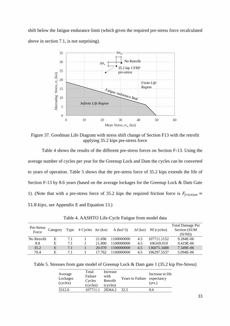
Figure 37. Goodman life diagram with stress shift change of section f13 with the retrofit
applying 35.2 kips pre-stress force .................................................................................... 33
Figure 38. Retrofit components and assembled cfrp retrofit ................................................... 35
Figure 39. Cross-section of pre-stress bearing mechanism with forces applied by bolts to create
the pre-stress ...................................................................................................................... 35
Figure 40. Cross-section view of retrofit friction grip mechanism .......................................... 35
Figure 41. Diagram of top view test setup and test matrix ...................................................... 37
Figure 42. Diagram of test-setup side view ............................................................................. 37
Figure 43. Test setup ................................................................................................................ 37
Figure 44. 3-d of the specimen with attachment plates, load, and boundary condition........... 38

Figure 45. Section 13 specimen fabrication details ................................................................. 39
Figure 46. Boundary conditions for abaqus simulation of test setup ....................................... 40
Figure 47. A) stresses from submodel of lock gate; b) stresses from model of test specimen 40
Figure 48. A) strain gage location; b) specimen with attached strain gages............................ 41
Figure 49. Dye penetrant application steps (ovouba, 2017) .................................................... 41
Figure 50. Notch at weld corner (8 million cycles) ................................................................. 42
Figure 51. Recorded strains, a) pre-notch; b) post-notch ......................................................... 42
Figure 52. Dye penetrant progression: a) 6 million cycles; b) 10 million cycles .................... 43
List of Tables
Table 1. List of gates on the arkansas river system, completed date, and date of repair ........... 3
Table 2. Types of cfrp based on modulus of elasticity and strength (kopeliovich, 2012) ....... 11
Table 3. Fatigue damage calculations of critical sections........................................................ 21
Table 4. Aashto life-cycle fatigue from model data ................................................................ 33
Table 5. Stresses from gate model of greenup lock & dam gate 1 (35.2 kip pre-stress) ......... 33

Notation
The following terms are used in the text of this report:
γ = fatigue load factor;
∆f = live load stress range due to the passage of the fatigue load;
∆𝐹𝑛 = nominal fatigue resistance;
∆𝐹𝑇𝐻 = constant amplitude fatigue threshold;
𝐴 = detail category AASHTO Table 6.6.1.2.3-1 (𝑘𝑠𝑖3);
𝑁 = number of expected cycles to reach the nominal fatigue resistance;
𝐷𝑖 = total damage;
𝑛𝑖 = number of cycles;
𝑁𝑖 = number of cycles to failure;
∆𝜎 = applied stress range;
𝑆𝑒 = fatigue endurance limit;
𝑆𝑒′ = estimated fatigue endurance limit;
𝑘 = modification factors in the Marin Equation;
Ω = unit of electrical resistance;

Disclaimer
The contents of this report reflect the views of the authors, who are responsible for the
facts and the accuracy of the information presented herein. This document is disseminated
under the sponsorship of the U.S. Department of Transportation’s University Transportation
Centers Program, in the interest of information exchange. The U.S. Government assumes no
liability for the contents or use thereof.

1
1. Introduction
1.1. Overview
Locks are essential for waterway transport along many river and canal systems,
allowing passage of ships through regions of differing water elevation. Locks operate by
creating a chamber of water that can be lowered or raised independently from the upstream or
downstream elevations. Figure 1 shows a typical miter lock gate and the water elevation
change process. As shown in Figure 1, two sets of gates open and close in sequence as the ship
transitions to a higher water elevation.
Figure 1. Function of lock gates within the lock system. 1) The lower gate is lowered
allowing entrance to the lock. 2) The lower gate closes and the water level changes. 3) The
upper gate opens allowing the vessel access to the higher water elevation.
The United States waterway transportation infrastructure (including lock gates) is
extensive, including over 12,000 miles of waterway (see Figure 2), and has economic, security,
and environmental benefits over traditional rail or highway transport systems (U.S. Army
Corps of Engineers, 1999). Other forms of transport such as rail or truck can be 5-10 times
more expensive than waterway transport respectively (see Figure 3) (The Port of Pittsburgh
Commision, 2017). As an example, barge transport along inland waterways of the upper

2
Mississippi River generates a transportation cost savings of nearly $1 billion dollars annually
(U.S. Army Corps of Engineers Mississippi Valley Division, 2016). The most common type of
barge used to transport goods along the major waterways is a 15-barge tow, which is equivalent
to nearly 5 unit trains and 870 trucks (see Figure 4)
Figure 2. Marine highway routes within the US (MARAD, 2017)
Figure 3. Transportation costs per ton (Port of Pittsburg, 2014)
Figure 4. Cargo capacity equivalency (US Army Corps, 2017)

3
While locks are essential to waterway transport, many of the lock gates within the
United States have reached or exceeded their design life. Many of the existing lock gates were
designed for a service life of 50 years (U.S. Army Corps of Engineers, 2017) but have aged
beyond this service-life expectancy, with additional locks getting older each year. Some locks
have even doubled their expected service life, having been constructed in the early 1900’s. The
Hiram M. Chittenden Locks in Seattle, Washington, will turn 100 years old in 2017. As lock
gates reach their design life, costly repairs are often needed to maintain waterway access. Table
1 shows, the scheduled repairs for the locks on the Arkansas River System, with required
repairs occurring after forty years of service (on average) (U.S. Army Corps of Engineers,
2017).
Table 1. List of gates on the Arkansas River System, completed date, and date of repair
Lock/Dam Started/Completed Repairs
Years Before
Repairs (yrs.)
Arthur V. Ormond Lock and Dam No. 9 1965/1969 N/A N/A
Choteau Lock No. 17 1967/1970 2012 42
Dardanelle Lock and Dam No. 10 1957/1969 2017 48
David D. Terry Lock and Dam No. 6 1965/1968 2009 41
Emmett Sanders Lock and Dam No. 4 1964/1968 N/A N/A
J. W. Trimble Lock and Dam No. 13 1965/1969 N/A N/A
Joe Hardin Lock and Dam No. 3 1963/1968 2013 45
Lock and Dam No. 5 1964/1968 N/A N/A
Montgomery Point Lock and Dam 1998/2004 2015 11
Murray Lock and Dam No. 7 1964/1969 2015 46
Newt Graham Lock No. 18 1967/1970 N/A N/A
Norrell Lock and Dam No. 1 1963/1967 N/A N/A
Norrell Lock No. 2 1963/1968 2013 45
Ozark-Jeta Taylor Lock and Dam No. 12 1964/1969 N/A N/A
Robert S. Kerr Lock and Dam No. 15 1964/1970 N/A N/A
Toad Suck Ferry Lock and Dam No. 8 1965/1969 Canceled Canceled
W. D. Mayo Lock No. 14 1966/1970 2014 44
Webber Falls Lock and Dam No. 16 1965/1970 2016 46
Average age before repair 40
Unscheduled repairs often increase as gates age, having a local economic impact on
freight transport and creating economic ripples throughout the national infrastructure.
Regarding the economic impact of service interruptions, temporary structural repairs to the
Montgomery Lock & Dam on the Ohio River totaled over $3.5 million, and were intended as

4
a short term solution only to last 5 years (Hawk 2011). Note that this $3.5 million cost does
not include the economic losses associated with transport rerouting. Lock gate fatigue failures
in the Algiers Lock along the Mississippi River resulted in $5.2 million of required repairs, and
interrupted waterway transport (McKee 2013). Aging of existing locks and service
interruptions can ripple through other aspects of our nation’s infrastructure. For example, aging
locks along the Mongongahela River Navigation System facilitate transport of approximately
20M tons of cargo annually (most of which is coal to generate electric power), with the
potential for a significant economic and power-grid impact given a gate failure or unscheduled
maintenance closure (Hawk 2011). An unscheduled extension of repairs on the Greenup Lock
and Dam (which occurred during winter months) caused energy plants to ship coal by alternate
means as stockpiles became depleted (Glass, 2012). During these extended repairs on the
Greenup Lock and Dam the MEMCO Barge Line company lost $1.3 million (Glass, 2012).
Fatigue and corrosion are key causes of lock gate component failures leading to
unscheduled service interruptions. Fatigue damage occurs as structural components are
subjected to frequently repeated loads, which in the case of a lock gate may include frequent
water elevation changes or gate openings. Figure 5 shows a typical miter gate section and
water elevation changes that occur during normal operation. Specific parameters leading to
fatigue damage include the applied component stress range ( 𝜎𝑎), applied mean stress (𝜎𝑚), as
well as the aggressiveness of the structural environment. Typically, increases in stress range,
mean stress, or the aggressiveness of the environment will lead to increased fatigue damage.
Submerged water environments where lock gates are required to operate, promotes corrosion
and unlike many other steel structures subjected to repeated loading, corrosion promoted
fatigue does not have a fatigue limit, so failures are difficult to predict (NACE International,
2017). Fatigue tends to occur first in connection details, especially those containing welds, due
to locked-in residual stresses or geometry induced stress concentrations which shift locally the

5
applied mean stress. Lock gates are primarily constructed of welded steel sections and many
gates are at high risk for fatigue failures following years of service in a corrosive environment
(U.S. Army Corps of Engineers, 2017).
Figure 5. Elevation view of Greenup Lock and Dam geometry
Additionally, lock gates are partially submerged in water which can make it difficult to
detect existing cracks. Because of this, existing cracks are often allowed to grow until failure
disrupts normal gate service. Once a gate has experienced cracking and needs repair, the lock
must be de-watered to allow access and favorable repair conditions.
The difficulty of crack detection and high repair costs have led to research on lock gate
fatigue cracking and failures. Carbon fiber reinforced polymer (CFRP) materials have been
used successfully as a crack mitigation method as they have a high strength to weight ratio,
high resistance to environmental corrosion, and a high ease of onsite implementation (Prem
Pal Bansal, 2016) (Alaa AL-Mosawe, 2015). Additional CFRP research involving post-
tensioned retrofits seems promising. Post-tensioned CFRP has been used in two different
applications: 1) bonded to existing cracks, like a patch (Prem Pal Bansal, 2016) (Alaa AL-
6
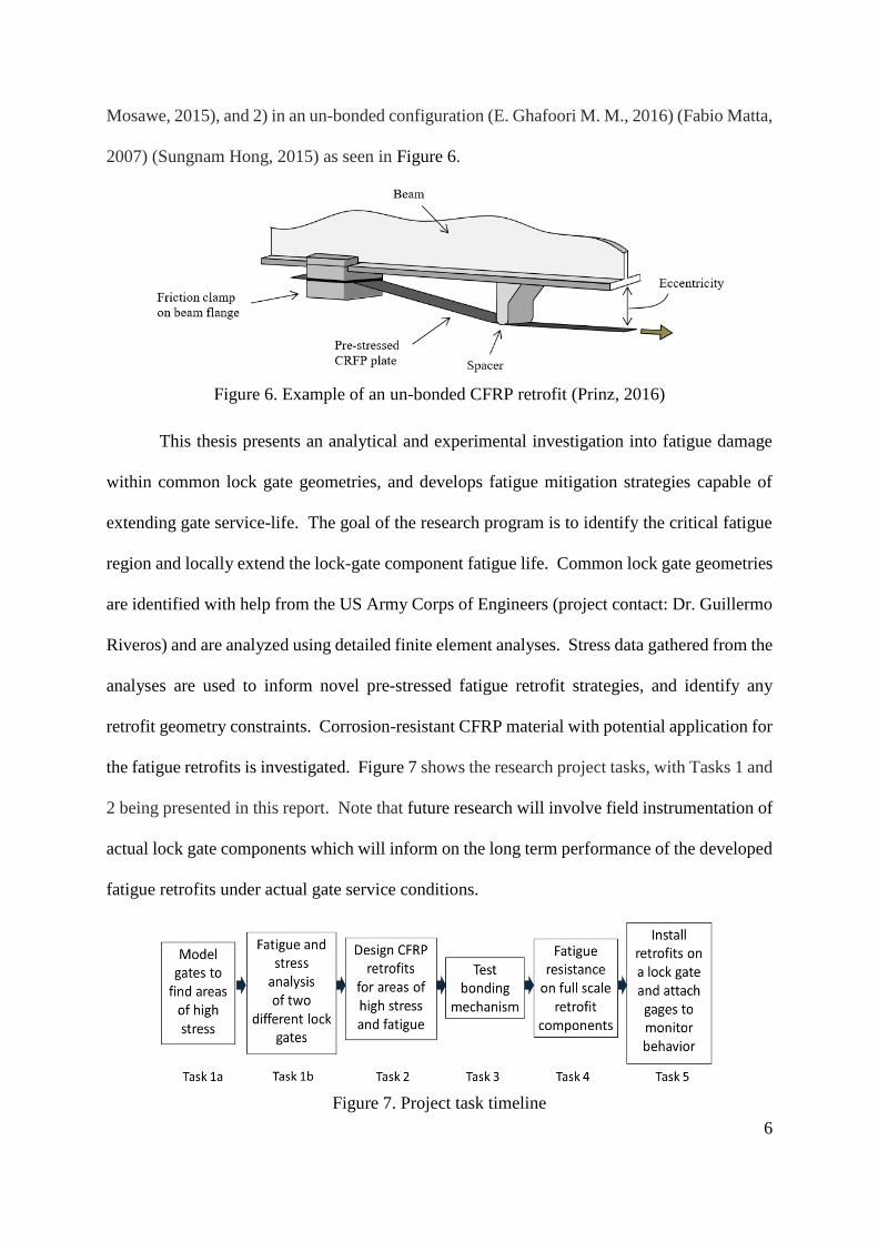
Mosawe, 2015), and 2) in an un-bonded configuration (E. Ghafoori M. M., 2016) (Fabio Matta,
2007) (Sungnam Hong, 2015) as seen in Figure 6.
Figure 6. Example of an un-bonded CFRP retrofit (Prinz, 2016)
This thesis presents an analytical and experimental investigation into fatigue damage
within common lock gate geometries, and develops fatigue mitigation strategies capable of
extending gate service-life. The goal of the research program is to identify the critical fatigue
region and locally extend the lock-gate component fatigue life. Common lock gate geometries
are identified with help from the US Army Corps of Engineers (project contact: Dr. Guillermo
Riveros) and are analyzed using detailed finite element analyses. Stress data gathered from the
analyses are used to inform novel pre-stressed fatigue retrofit strategies, and identify any
retrofit geometry constraints. Corrosion-resistant CFRP material with potential application for
the fatigue retrofits is investigated. Figure 7 shows the research project tasks, with Tasks 1 and
2 being presented in this report. Note that future research will involve field instrumentation of
actual lock gate components which will inform on the long term performance of the developed
fatigue retrofits under actual gate service conditions.
Figure 7. Project task timeline

7
2. Review of Relevant Literature
2.1. Fatigue in Steel Lock Gates and Review of Analysis Methods
Lock gates are prone to fatigue cracking due to the severity of the applied cyclic loads
and aggressiveness of the corrosive environment. Connection regions where members are
welded, bolted, and contain irregular geometric features often create stress concentrations that
lead to high stress fluctuations and fatigue damage. Figure 8 shows how stress concentrations
can develop around geometric features, as the stresses “flow” around geometric features
(Anderson, 2005). Welded sections also tend to be more susceptible to fatigue cracking as they
introduce heat-induced flaws in the metal microstructure. (Mertz, 2012).
Figure 8. Stress flow and concentration around a hole (adapted from figure in (Anderson,
2005))
While it can be difficult to account for local geometric features and their effects on local
stress ranges, the American Association of State Highway Transportation Officials (AASHTO)
has developed common component details and their corresponding fatigue capacities based on
applied nominal stresses (American Association of State Highway and Transportation
Officials, 2012). The detail categories (A, B, B’, C, C’, D, E, and E’) found in (American
Association of State Highway and Transportation Officials, 2012) are determined based largely
on experimental testing of different component geometries. All fatigue detail capacities take
the form of Equation 1:
(∆𝐹)𝑛 = (𝐴/𝑁)1
3 Equation 1
where 𝐴 is a constant representing the intercept of the stress versus number of cycles to failure
(S-N) curve taken from AASHTO Table 6.6.1.2.5-1 based on the detail type; 𝑁 is the number

8
of expected cycles to reach the nominal fatigue resistance ((∆𝐹)𝑛) (American Association of
State Highway and Transportation Officials, 1988).
2.2. Review of Fatigue Retrofit Methods
There are many different fatigue retrofit methods currently in use; however, all methods
aim to do one of two things: 1) reduce the applied component stress range (often by stiffening
or softening the section), or 2) reduce the applied component mean stress (often through an
induced pre-stress). Common methods include weld surface treatments, hole-drilling, vee-and-
weld, adding doubler/splice plates, and post-tensioning. The following sections give a review
of each of these methods.
2.2.1. Weld Surface Treatment
Surface treatments improve un-cracked weld strength by reducing abrupt geometric
changes or removing locked-in tensile residual stresses. Surface treatments include grinding,
gas tungsten arc or plasma re-melting of the weld toe, and impact treatments. Surface
treatments improve fatigue strength by improving the weld geometry and reducing stress
concentrations, eliminating discontinuities where fatigue cracks may propagate, and reducing
residual tensile stresses. After the surface treatment has been applied, the damaging effects of
any prior loading cycles are removed, and the next greatest S-N curve can be used to predict
the life of the section. Surface treatments only affect the weld toes (Robert J. Dexter, 2013).
1.1.1. Hole-Drilling in Steel Sections
Hole drilling is a common method for alleviating high stress concentrations at the tip
of existing fatigue cracks. This method incorporates fatigue analysis fundamentals, by
removing the sharp notch at the crack tip, stopping the propagation of the crack under Mode 1
loadings but less effective for mixed mode loading. The hole also lessens the stress
concentration by shifting the stresses around the sides of the hole, see again Figure 8. The hole
size must be large enough to contain the full crack tip with required hole sizes sometimes

9
ranging between 2-4 inches (Robert J. Dexter, 2013). The hole drilling method is a simple way
of slowing down crack growth by re-directing the stress path.
2.2.2. Vee-and-Weld
The vee-and-weld method is often used in conjunction with other methods to reduce
the actual stress range experienced by the original crack (Robert J. Dexter, 2013). Once a crack
has been found, the area around the crack length is removed in a “V” shape and then refilled
with weld metal, see Figure 9. One drawback of this method is that the weld must be done by
a certified welder, and significant care must be taken to produce a quality weld. Additionally,
studies conducted on the vee-and-weld method concluded that the resulting repaired fatigue
life is only as good as the original detail (Robert J. Dexter, 2013) (Stefano Caramelli, 1997)
(Kentaro Yamada, 1986)
Figure 9. Vee and weld fatigue repair method
2.2.3. Doubler/Splice Plates
The addition of doubler or splice plates near fatigue prone details aim to reduce the
applied stress range within the original component (Robert J. Dexter, 2013) . As the section
area increases, the applied stress range is reduced (see Figure 10) and fatigue life is extended.
One of the drawbacks of the doubler/splice plate method is the significant addition of weight
to the structure.
2.2.4. Post-Tensioning
Fatigue cracks form by repeated stresses in tension causing a section to open and close.
Post-tensioning considers the tensile stresses needed to create and propagate cracks by shifting

10
the effective mean stress into a region of slight compression. Pre-stressed retrofits are placed
on the section and introduce the tension required to shift the mean stress, see Figure 10. There
are different methods to apply post-tension: pre-stressing strands, post-tensioning bars, or nuts
torqued on high-strength rods. All the previously stated methods add tension to shift the
effective mean stress partly or completely into compression (Robert J. Dexter, 2013).
Figure 10. Stress amplitude reduction (Doubler/Splice Plates) and Shifted Mean Stress (Post-
Tensioning)
2.3. Overview of CFRP and Review Applications in Structural Retrofits
CFRP is a composite material made of carbon fiber strands within a resin matrix, see
Figure 11. As seen in Figure 11, the carbon fiber strands are laid laterally and longitudinally.
The weave pattern allows CFRP to be flexible and moldable while still having significant
strength in tension. Additionally, CFRP is corrosion resistant and has a high fatigue life. There
are different types of CFRP with varying properties allowing for a broader use of the material.
Table 2 gives a list of five of the most readily available types of CFRP. CFRP is currently used
within different fields including the automotive, aerospace, sporting goods, and infrastructure
because of its strength, flexibility, corrosion resistance, high strength to weight ratio, and
moldability.

11
Figure 11. Section view diagram of CFRP
Table 2. Types of CFRP based on modulus of elasticity and strength (Kopeliovich, 2012)
Type Main Property
Ultra-High Modulus (UHM) Modulus of Elasticity: >65,400 ksi
High Modulus (HM) Modulus of Elasticity: 51,000-65,400 ksi
Intermediate Modulus (IM) Modulus of Elasticity: 29,000-51,000 ksi
High Tensile, Low Modulus (HT) Tensile Strength: >436 ksi
Modulus of Elasticity: <14,500 ksi
Super High Tensile (SHT) Tensile Strength: >650 ksi
Recently CFRP has been introduced as a strength and crack reduction retrofit in
concrete and steel sections. CFRP has been used in concrete as a wrap-like retrofit to improve
the tensile capacity of the section, see Figure 12. Current research has been conducted to
determine the capacity of CFRP compared to steel and see how it works as a fatigue or
strengthening retrofit (E. Ghafoori M. M., 2016) (Fabio Matta, 2007) (M. Tavakkolizadeh,
2003). The elastic modulus of CFRP is similar to that of steel, but CFRP has a higher ultimate
strength, see Figure 13. CFRP is less prone to corrosion than steel and has a lower weight to
strength ratio (CFRP is about 20% of the mass of steel but with the same strength and elastic
modulus (Alkhrdaji, 2015)). Several studies have shown the advantages of using CFRP to
increase flexural performance, by reinforcing tensile components, and extending fatigue life,
by reducing the stress range or shifting the mean stress down (A. Peiris, 2015) (D. Schnerch,
2008) (T.C. Miller, 2001) (B. Kaan, 2012) (Y. Huawen, 2010) (E. Ghafoori M. M., 2015)
(Hussam Mahmoud, 2017).

12
Figure 12. Bonded CFRP strips used to strengthen concrete structure (Alkhrdaji, 2015)
Figure 13. CFRP vs Steel elastic modulus
Pre-stressed CFRP has successfully been used, by Ghafoori et al (2016), to shift the
mean stress in railroad bridges below the fatigue endurance limit increasing fatigue life.
Research has proven that pre-stressed CFRP has increased the fatigue life of a steel section by
up to 20 times (E. Ghafoori M. M., 2011) (Y. Huawen, 2010) with the thickness and pre-stress
level of the CFRP being two important factors that influence how the retrofit performs. The
current research aims to develop CFRP retrofits to reinforce critical fatigue details on lock
gates.

13
3. Analytical Investigation into Lock Gate Component Fatigue
3.1. Selection of Lock Gate for Analysis
The selection of lock gates for analysis in this thesis were conducted with the assistance
of the Army Corps of Engineers; the Corps oversees 239 lock systems throughout the United
States. All lock gates considered are in-service, and in difficult environments to study without
dewatering. The gate selection for this research project was based on maintenance and
dewatering schedules of existing gates in conjunction with the project timeline. One gate
selected for this project was the Greenup Lock and Dam on the Ohio River.
3.2. Modeling Techniques
3.2.1. Geometry and Boundary Conditions
A detailed finite element model considering local geometric features was created from
construction documents obtained for the Greenup Lock and Dam on the Ohio River. All
boundary conditions considered represent the operation of the constructed gate. The gate was
modeled using the commercial finite element software ABAQUS (Abaqus, 2017). Only one
side of the lock gate was modeled due to symmetry. The dimensions of the gate are 63.5 feet
by 61.5 feet by 5.71 feet, see Figure 14 and Figure 15. The gate was constructed from Grade
50 steel sections welded together. The gate diagonals (constructed from pre-tensioned rods)
were simulated using linear spring elements pre-stressed to 22.9 ksi following the gate
construction documents.

14
Figure 14. Upstream elevation and top view of a lock gate (Greenup Lock and Dam, Ohio
River)
Figure 15. Section through leaf and recess of Lock Gate #1 (Greenup Lock and Dam, Ohio
River)
Shell elements were used to simulate the gate geometric features. A general mesh size
of 2.5inches was used throughout, balancing computation expense and stress accuracy near
geometric features having high stress gradients. In locations where the diagonal spring
elements connect to the gate structure, nodes were tied to create rigid body regions simulating
the details seen in Figure 16, and avoid local stress concentrations at the spring gate attachment.
At the gudgeon pin and pintle (see again Figure 14) nodes were tied to create rigid bodies to

15
simulate the quoin blocks that are the point of rotation (shown in construction details of Figure
17 and Figure 18).
Boundary conditions chosen followed previous analyses performed by (Riveros, 2009).
The boundary conditions were added to the following sections: the gudgeon pin was restrained
in the X and Y directions as shown in Figure 19; the quoin and lock ends were restrained in the
Y and Z directions; and the pintle was restrained in the X, Y, Z, XR, and YR, see Figure 19.
The boundary conditions on the quoin and miter ends were applied along the full length of the
gate. The quoin and miter end boundary conditions restrict movement in the X and Y directions
simulating the concrete dam on the quoin end and the other lock gate leaf on the miter end, see
Figure 19 and Figure 20.
Figure 16. Lock Gate #1: detail of diagonal connection
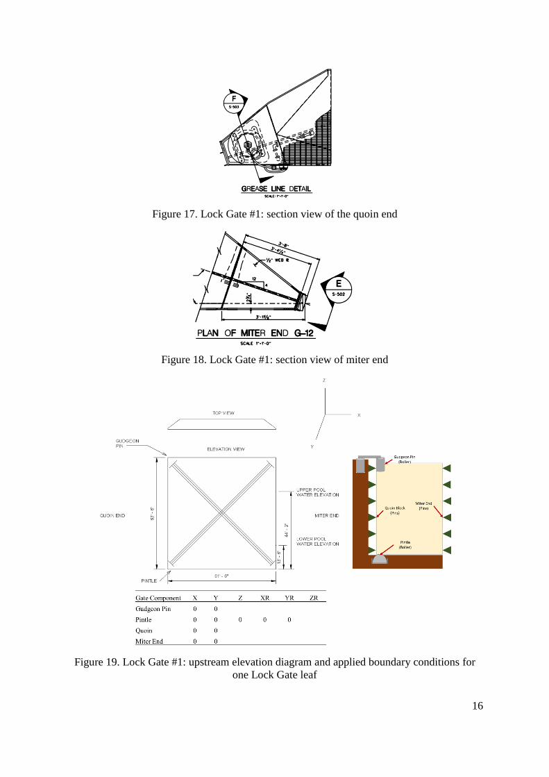
16
Figure 17. Lock Gate #1: section view of the quoin end
Figure 18. Lock Gate #1: section view of miter end
Figure 19. Lock Gate #1: upstream elevation diagram and applied boundary conditions for
one Lock Gate leaf

17
Figure 20. Lock gate in empty lock
3.2.2. Loading
All gate analyses consider gravity and hydrostatic loading. Changing water levels
during lock operation are modeled using hydrostatic loads applied in sequential amplitudes to
simulate a continuous rising water elevation. The load on the downstream face was set at the
highest water level and remained constant during the analyses (see Figure 21). In Figure 21 the
varying hydrostatic pressures applied to the upstream face are illustrated as a sequence of
applied triangular ramping loads which provide a constantly increasing hydrostatic pressure
corresponding to the increasing water level. The various load amplitudes turn one load on and
off at different analysis “steps”; however, the magnitude of any two amplitudes always adds to
one, allowing smooth transition from elevation to elevation.
Figure 21. Different hydrostatic load levels applied on the gate (ft. – in.) and simulation of
water level elevation change through hydrostatic load amplitude triggering
Concrete
Dam
Miter
End
Quoin
End

18
3.3. Determination of Fatigue Damage
The purpose of the gate model is to determine regions of high fatigue susceptibility.
This is achieved by first identifying regions of high local stress fluctuation. As seen in Figure
22, high-stress regions can be determined from stress contours. The regions of high stress are
compared to the AASHTO fatigue categories considering nominal applied stress ranges.
Twenty-seven sections were determined to have high-stress concentrations. These sections are
presented in Appendix A.
Figure 22. Greenup Lock and Dam von Misses Stress contour and numbered sections of high
stress concentrations with stress graphs
3.3.1. Miner’s Total Damage
The damage caused by one water elevation-change cycle for each gate component was
determined using Miner’s linear damage accumulation rule (referred hereafter as Miner’s rule).
When using Miner’s rule, higher stress ranges cause greater fatigue damage and fatigue damage
is inversely related to the fatigue capacity. Miner’s rule is presented in Equation 4:
∑𝐷𝑖 = ∑𝑛𝑖
𝑁𝑖 Equation 4

19
where 𝐷𝑖 is the total damage, 𝑛𝑖 is the number of cycles, and 𝑁𝑖 is the number of cycles to
failure. 𝑁𝑖 can be calculated from the AASHTO fatigue capacity equation, here re-arranged as
Equation 5:
𝑁𝑖 = 𝐴 ∗ (∆𝜎)−3 Equation 5
where 𝐴 is the detail category acquired from AASHTO Table 6.6.1.2.3-1, and ∆𝜎 is the applied
stress range (determined from the finite element simulations).
3.3.2. Cycle Counting
In order to evaluate fatigue damage using Equations 4 and 5, stress cycle counts and
corresponding stress ranges from the analyses must be known. Two common methods of cycle
counting are the rain-flow counting method and the reservoir method (see Appendix B for
details on each method). Based on the graphs generated from the stress-time data (shown in
Figure 22), the reservoir method was chosen and the amount of damage per section was
calculated using Miner’s Rule.

20
4. Results and Discussion from Gate Analyses
The fatigue analyses conducted for this research use the stress based method provided
by AASHTO and Miner’s linear damage accumulation rule. Note that the AASHTO stress
based method has been used successfully to design fatigue prone bridge components
(American Association of State Highway and Transportation Officials, 1988).
4.1. Fatigue Life Evaluation
Table 3 presents the accumulated fatigue damage during water-elevation change
throughout the various gate components. From Table 3, and based on the applied stress range
and detail category, Section F13 of Figure 22 accumulates the most fatigue damage during one
water-elevation change cycle. Figure 23 shows the von Mises stress concentrations within the
gate (at the stage of largest water elevation difference) along with the welded connection detail
for the area with the highest fatigue damage.
Figure 23. von Misses Stress concentrations at the point of highest loading and the
connection detail for the section
Section F13 was similar in detail to sections F7-F11, F13-F14, and F20. These sections
were all characterized as having the same detail category, AASHTO detail category E, but
Section F13 was identified as the area of highest fatigue damage due to a high-stress
concentration coupled with a small cross-sectional area when compared to the other detail

21
sections on the gate. Section F13 is also situated in the middle near the bottom of the gate where
the hydrostatic pressure difference is the greatest. Section F13 also has a smaller cross-sectional
area than section F20 (the point of highest hydrostatic pressure).
Table 3. Fatigue damage calculations of critical sections
Location Category Type
No.
Cycles Δσ A (ksi^3)
Δf
(ksi) Nf (cycles)
Damage
(N/Nf)
Total Damage
Per Section
Section F7 E 7.1 1 5.945 1.10E+09 4.5 5.235E+06 1.910E-07 1.910E-07
Section F9 E 7.1 1 7.093 1.10E+09 4.5 3.082E+06 3.244E-07 3.244E-07
Section F10 E 7.1 1 22.732 1.10E+09 4.5 9.364E+04 1.068E-05 1.068E-05
Section F11 E 7.1 1 22.52 1.10E+09 4.5 9.631E+04 1.038E-05 1.038E-05
Section F12 E 7.1 1 21.584 1.10E+09 4.5 1.094E+05 9.141E-06 9.141E-06
Section F13 E 7.1 1 23.444 1.10E+09 4.5 8.537E+04 1.171E-05 1.171E-05
Section F14 E 7.1 1 23.301 1.10E+09 4.5 8.695E+04 1.150E-05 1.150E-05
Section F15 E 7.1 1 22.022 1.10E+09 4.5 1.030E+05 9.709E-06 9.709E-06
Section F16 E 7.1 1 9.807 1.10E+09 4.5 1.166E+06 8.574E-07 8.574E-07
Section F17 E 7.1 1 9.807 1.10E+09 4.5 1.166E+06 8.574E-07 8.574E-07
Section F20 E 7.1 1 22.411 1.10E+09 4.5 9.773E+04 1.023E-05 1.023E-05
Section F21 E 7.1 1 21.916 1.10E+09 4.5 1.045E+05 9.570E-06 9.570E-06
Section F22 E 7.1 1 19.854 1.10E+09 4.5 1.406E+05 7.114E-06 7.114E-06
Section Inside 1 D 1.5 1 12.534 2.20E+09 7 1.117E+06 8.950E-07 8.950E-07
Section Inside 2 D 1.5 1 10.37 2.20E+09 7 1.973E+06 5.069E-07 5.069E-07

22
5. Description of Detailed Fatigue Investigation for Critical Component
While the nominal stress based approach in AASHTO is useful for comparing the
propensity for fracture between various details, more detailed fatigue investigations are useful
for understanding the underlying fatigue causes and identifying strategies for damage
prevention. For this purpose, a submodel of Section F13 is created to acquire more refined
stress data from solid element types (ABAQUS element type C3D8R) within the specific
section. The submodel boundary conditions are informed from the main gate model
deformations such that compatibility is ensured and the submodel represents the same loading
as provided for the entire gate model. Figure 24a) shows the Section F13 submodel integrated
with the larger gate model while Figure 24b) shows the submodel without the gate. In addition
to the refined stress data, the submodel allows simulation of weld geometry effects within the
component that are impractical to include in the larger-scale gate simulations. For the
submodel, section welds are modeled as triangular fillet welds, within the same submodel part,
corresponding to the construction documents provided (see Figure 25).
(a) (b)
Figure 24. a) A submodel embedded in gate model with mesh view; b) 3-D of submodel with
contours from loading applied to gate

23
Figure 25. Triangular (fillet) Weld geometry modeled as part of the solid element model
In addition to local geometric features, the submodel considers a more refined mesh of
0.25in for capturing detailed stress information within regions having high stress gradients.
Note that the main gate model had a mesh size equal to 2.5in.
A mesh convergence study helped determine the appropriate mesh size for the
submodel used in this study, balancing computational expense and accuracy. In the mesh
convergence study, mesh sizes at 0.25in, 0.13in, and 0.1in resulted in similar stresses (less than
0.3% difference) near the component corner (see again Figure 24(b)) indicating that the
considered 0.25in mesh fully captures the stress gradient present in the component detail.
5.1. Fatigue Endurance from Constant Life Diagrams: The Goodman Criterion
Different from the nominal stress analysis using the AASHTO detail categories, local
stress-states within the gate component (as informed by the submodel) can help determine
fatigue damage from interacting mean stresses and stress ranges. This information is helpful
in identifying strategies for fatigue mitigation within local component regions. Constant life
diagrams provide the mean stress and stress range interactions for determining the fatigue
endurance limit, with the Goodman criterion (see Equation 6) being commonly used for low
carbon structural steels. In Equation 6, Se is the fatigue endurance limit (having zero mean
stress), Sult is the material ultimate strength, and a and m are the stress range and mean stress
as provided in Equation 6 and Equation 7 respectively.

24
1ult
m
e
a
SS
Equation 6
𝜎𝑚 =𝜎𝑚𝑎𝑥+𝜎𝑚𝑖𝑛
2 Equation 7
𝜎𝑎 = 𝜎𝑚𝑎𝑥 + 𝜎𝑚𝑖𝑛 Equation 8
In Equations 7 and 8, 𝜎𝑚𝑎𝑥 is the maximum stress while 𝜎𝑚𝑖𝑛 is the minimum stress,
experienced during the loading cycles. The fatigue endurance limit (𝑆𝑒) was determined using
the Marin equation, shown in Equation 9 (Marin, 1962).
𝑆𝑒 = 𝑘𝑎𝑘𝑏𝑘𝑐𝑘𝑑𝑘𝑓𝑆𝑒′ . Equation 9
where the modification factors 𝑘𝑎, 𝑘𝑏 , 𝑘𝑐, 𝑘𝑑 , and 𝑘𝑓 are respectively based on surface
condition, size, load, temperature, reliability, and miscellaneous effects. 𝑆𝑒′ is estimated using
Equation 10 given by (Shigley & Mischke, 1989).
𝑆𝑒′ = {
0.5 ∗ 𝑆𝑢𝑙𝑡 𝑆𝑢𝑙𝑡 ≤ 200 𝑘𝑠𝑖100 𝑘𝑠𝑖 𝑆𝑢𝑙𝑡 > 200 𝑘𝑠𝑖
Equation 10
The calculated fatigue endurance limit for the lock gate components in this study
is 𝑆𝑒 = 18.8 𝑘𝑠𝑖. The detailed procedure used to determine 𝑆𝑒 and the modification factors is
provided in Appendix C.
For graphical reference, Figure 26 shows the various stress components used in the
Goodman criterion and Figure 27 shows an example Goodman constant life diagram bound the
yield stress, referred to as a “modified” Goodman diagram. In Figure 27, the yield stress bound
prevents fatigue infinite life determination under high plasticity, as different fracture
mechanisms participate in the damage. Note also in Figure 27, that m – a combinations that
fall underneath the modified Goodman diagram line result in an infinite fatigue life, prior to
corrosion effects.
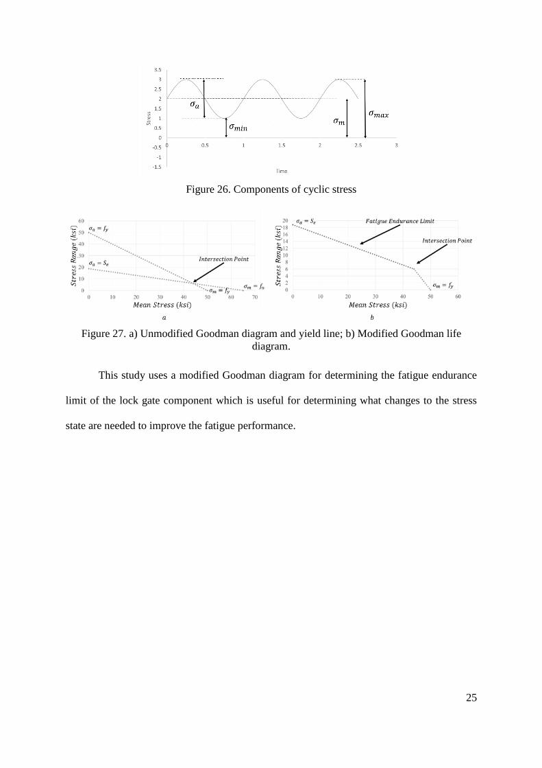
25
Figure 26. Components of cyclic stress
Figure 27. a) Unmodified Goodman diagram and yield line; b) Modified Goodman life
diagram.
This study uses a modified Goodman diagram for determining the fatigue endurance
limit of the lock gate component which is useful for determining what changes to the stress
state are needed to improve the fatigue performance.

26
6. Required Pre-Stressing Force from Goodman Constant Life Diagram
Figure 28 shows the Goodman life diagram created using the data from the submodel
and 𝑆𝑒 = 18.8 𝑘𝑠𝑖. The max principal stress data from the submodel is analyzed to determine
a max amplitude and mean stress using Equations 7 and 8. Section F13 has a maximum mean
stress of 22.32 ksi and a maximum stress range amplitude of 21.58 ksi resulting in a finite
fatigue life (as expected) as shown on the diagram (note in Figure 28 the values fall outside the
Goodman line). The stress data from the submodel corresponds to one water change cycle
(lockage); however, the Lockages are repeated thousands of times throughout a year, and over
a period of 50 years (the design life of the gate), the amount of cycles the section experiences
outside of the fatigue endurance limit can lead to cracking.
This Goodman diagram is useful in determining the required mean stress shift such that
the component falls within the Goodman line and experiences infinite fatigue life, regardless
of past damaging cycles. The retrofit strategy taken herein considers an external applied pre-
stress such that the mean stress shift transitions the stress state to the edge of the endurance
limit. The total amount of pre-stress needed for this can be found by calculating the m change
needed on the Goodman diagram. As a bonus, when the mean stress shifts the amplitude of the
stress range also decreases as 40% of the compressive stress cycles are not considered in the
fatigue evaluation (Eurocode 3: Design of Steel Structures - Part 1-9: Fatigue, 2005). Figure
28 shows the shift in the mean stress along with the reduction of amplitude which is calculated
to be Equation 11.
𝜎𝑎𝑓 =𝜎𝑚𝑎𝑥−(𝜎𝑚𝑜−𝜎𝑚)−((𝜎𝑚𝑖𝑛+1)−(𝜎𝑚𝑜−𝜎𝑚))∗60%
2 Equation 11
In Equation 11, 𝜎𝑚𝑎𝑥is the maximum principle stress from the submodel analysis, 𝜎𝑚𝑜is
the initial mean stress, 𝜎𝑚𝑖𝑛is the minimum principle stress from the submodel analysis, 𝜎𝑚 is
the new mean stress, and 𝜎𝑎𝑓 is the newly calculated amplitude stress. The change in mean

27
stress, ∆𝜎𝑚, for gate Section F13 (based on the submodel analysis) is calculated to be 18.78ksi
(which is rather large).
Figure 28. Modified Goodman Life Diagram with data point and stress shift
The required tension force to shift the mean stress by 18.78ksi can be found from the
geometry of section and pre-stress application strategy. A free body diagram of the pre-stress
retrofit configuration considered is shown in Figure 29. In Figure 29, steel plates clamp to the
gate section and a pre-stressing force applied at an eccentricity (e) from the gate section.
Equation 12 calculates the pre-stress force, based on the resulting section stress, pre-stress
force, applied moment (from the eccentricity), and section area.
Fprestress =∆σm
(e∗tp
2∗I)+(
1
A) Equation 12
In Equation 12, 𝐹𝑝𝑟𝑒𝑠𝑡𝑟𝑒𝑠𝑠 is the pre-stress force, ∆𝜎𝑚 is the change in stress, 𝑒 is the
moment arm, 𝑡𝑝 is the thickness of the gate component, 𝐼 is the moment of inertia, and 𝐴 is
the area of the plate. The pre-stress force is 𝐹𝑝𝑟𝑒𝑠𝑡𝑟𝑒𝑠𝑠 = 8.8 𝑘𝑖𝑝𝑠. The pre-stress force is
applied to the CFRP to shift the mean stress.

28
Figure 29. Free body diagram of the pre-stress force
6.1. Transfer of Pre-Stress through Friction Clamping
To transfer the required pre-stress into the gate component, a friction clamp is designed.
The free body diagram shown in Figure 30 is used to assist in the calculation of the friction
force, which is given by Equation 13:
𝐹𝑓𝑟𝑖𝑐𝑡𝑖𝑜𝑛 = 𝜇 ∗ 𝑁 Equation 13
where the static coefficient of friction is 𝜇, and 𝑁 is the normal force. The total required friction
force to avoid slippage of the retrofit is one half the required prestress force (see Appendices
D and E for additional calculations).
Figure 30. Free body diagram of clamp, retrofit, and section 13 to determine the required
friction force from known pre-stress force
The static coefficient of friction required in Equation 13 is dependent on the interaction
between surfaces. Corrosion changes the surface roughness of the steel plate, therefore the

29
static coefficient of friction for an un-corroded and corroded steel plate must be determined,
see Figure 31. As shown in Figure 32, an experiment was conducted to determine an estimate
for the static coefficient of friction between A36 steel and an uncorroded steel plate and a
corroded steel plate. The static coefficient of friction for stainless steel and an uncorroded steel
plate was 𝜇 = 0.297 and for a corroded steel plate was 𝜇 = 0.343, see Appendix D for the
derivation of static coefficient of friction.
Figure 31. Corroded (bottom) and uncorroded (top) steel surfaces
(a) (b)
Figure 32. Static coefficient of friction test: a) static coefficient of friction free body diagram;
b) test materials

30
7. Effect of Pre-Stress on Component Fatigue Susceptibility
To evaluate the effectiveness of the developed retrofit prestress, the designed pre-stress
level of 8.8kips is applied to the critical gate component (Section F13) in the full gate finite
element simulation. Figure 33 shows the application method for the pre-stress, involving
nonlinear springs and rigid body connection regions (simulating plate attachments). Stiffness
of the nonlinear springs considers high modulus CFRP (E = 51,000ksi). Also shown in Figure
33, the simulated pre-stress is applied in the horizontal and vertical directions at section F13.
In the simulation, the double configuration was chosen to counteract the multi-axial stresses
induced by the hydrostatic pressure difference on either side of the gate. Note that the nonlinear
springs are arbitrarily attached to the gate section 16-3/8 in. from the component corners that
experience the high stress concentration.
Resulting stress states within gate component indicate a slight reduction in mean stress
(see later “Prestress Simulation Results” section); however, the shift was lower than predicted
by the Goodman diagram and the component remained within the finite life region. This result
indicates that higher pre-stress values are need for significant fatigue life improvement and
suggests a revision is needed to the pre-stress force calculation.
Figure 33. Retrofit application on Section F13 in the FEA model

31
7.1. Revised Calculations Following Retrofit Simulations
The pre-stress calculations from Section 6 were based on stress shifts within a flat steel
plate; however, the geometry of the gate sections differ greatly from this assumption. A revised
calculation is needed that considers the entire Section F13 cross section as seen in Figure 34
and Figure 35. From the section stresses created from the free body diagram shown in Figure
35, the new cross-section requires a larger pre-stress force of 366.6 kips (nearly 42 times greater
than previously predicted). Note that this pre-stress level is required for infinite life; however,
given the large force required, increases to the finite life within the critical component may be
more practical.
Figure 34. New Pre-stress force cross-section
Figure 35. Free body diagram used to calculate the pre-stress force
As the required pre-stress force changes, the required friction force also changes due to
the increased required pre-stress force. The greater pre-stress force creates a greater normal
e ec
Mpre-stress
Fpre-stress
Fpre-stress

32
force, 𝑁 = 540 𝑘𝑖𝑝𝑠, see Appendix E for calculations. The increased normal force increases
the friction force to, 𝐹𝑓𝑟𝑖𝑐𝑡𝑖𝑜𝑛 = 183.6 𝑘𝑖𝑝𝑠 (with a 𝜇 = 0.34), see again Equation 13.
7.2. Pre-Stress Simulation Results
Figure 36 shows the effects of different pre-stress levels (8.8 kips, 35.2 kips, and 70.4
kips) on the stress range resulting from one lockage cycle. From Figure 36, the retrofit pre-
stress level of 8.8 kips does not significantly shift the applied mean stress to have any impact
on the component fatigue life. Higher pre-stress levels (arbitrarily chosen beyond 8.8kips) at
35.2 kips and 70.4 kips are capable of shifting the mean stress enough to move a portion of the
stress range into compression (see Figure 36) therein prolonging the component fatigue life.
Figure 36. Stress range shift, in Section F13, due to applied CFRP pre-stress (1 lockage
cycle)
Both the Goodman Life Diagram and the AASHTO life-cycle fatigue method were
implemented using the data from the 3 different pre-stress force analyses. The two different
methods help determine the effect of the retrofit on the stresses on gate Section F-13. Figure
37 shows a Goodman Life Diagram for Section F-13 with the mean and amplitude stresses of
the section with and without the retrofit pre-stress forces. While the pre-stress forces shift the
stress state in Section F13 towards the endurance limit, see Figure 37, the stress levels do not
-10
-5
0
5
10
15
20
25
0 10 20 30 40 50 60
Str
ess
(ksi
)
Analysis Step
Increasing
Pre-Stress
Level
Compression Zone
No Retrofit
8.8 kip pre-stress
35.2 kip pre-stress
70.4 kip pre-stress
DReduced
33
shift below the fatigue endurance limit (which given the required pre-stress force recalculated
above in section 7.1, is not surprising).
Figure 37. Goodman Life Diagram with stress shift change of Section F13 with the retrofit
applying 35.2 kips pre-stress force
Table 4 shows the results of the different pre-stress forces on Section F-13. Using the
average number of cycles per year for the Greenup Lock and Dam the cycles can be converted
to years of operation. Table 5 shows that the pre-stress force of 35.2 kips extends the life of
Section F-13 by 8.6 years (based on the average lockages for the Greenup Lock & Dam Gate
1). (Note that with a pre-stress force of 35.2 kips the required friction force is 𝐹𝑓𝑟𝑖𝑐𝑡𝑖𝑜𝑛 =
51.8 𝑘𝑖𝑝𝑠, see Appendix E and Equation 13.)
Table 4. AASHTO Life-Cycle Fatigue from model data
Pre-Stress
Force Category Type # Cycles Δσ (ksi) A (ksi^3) Δf (ksi) Nf (cycles)
Total Damage Per
Section (SUM
(N/Nf))
No Retrofit E 7.1 1 21.696 1100000000 4.5 107711.1152 9.284E-06
8.8 E 7.1 1 21.800 1100000000 4.5 106169.019 9.419E-06
35.2 E 7.1 1 20.070 1100000000 4.5 136075.3488 7.349E-06
70.4 E 7.1 1 17.762 1100000000 4.5 196297.5537 5.094E-06
Table 5. Stresses from gate model of Greenup Lock & Dam gate 1 (35.2 kip Pre-Stress)
Average
Lockages
(cycles)
Total
Failure
Cycles
(cycles)
Increase
with
Retrofit
(cycles)
Years to Failure
Increase in life
expectancy
(yrs.)
3312.6 107711.1 28364.2 32.5 8.6
0
5
10
15
20
25
30
35
0 10 20 30 40 50 60
Alter
nat
ing
Str
ess,
a
(ksi
)
Mean Stress, m (ksi)
No Retrofit
35.2 kip CFRP
pre-stress
Da
Dm
Infinite Life Region
Finite Life
Region
34
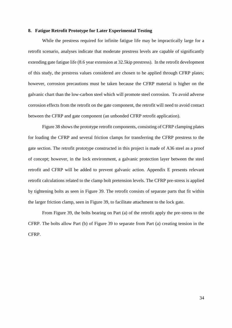
8. Fatigue Retrofit Prototype for Later Experimental Testing
While the prestress required for infinite fatigue life may be impractically large for a
retrofit scenario, analyses indicate that moderate prestress levels are capable of significantly
extending gate fatigue life (8.6 year extension at 32.5kip prestress). In the retrofit development
of this study, the prestress values considered are chosen to be applied through CFRP plates;
however, corrosion precautions must be taken because the CFRP material is higher on the
galvanic chart than the low-carbon steel which will promote steel corrosion. To avoid adverse
corrosion effects from the retrofit on the gate component, the retrofit will need to avoid contact
between the CFRP and gate component (an unbonded CFRP retrofit application).
Figure 38 shows the prototype retrofit components, consisting of CFRP clamping plates
for loading the CFRP and several friction clamps for transferring the CFRP prestress to the
gate section. The retrofit prototype constructed in this project is made of A36 steel as a proof
of concept; however, in the lock environment, a galvanic protection layer between the steel
retrofit and CFRP will be added to prevent galvanic action. Appendix E presents relevant
retrofit calculations related to the clamp bolt pretension levels. The CFRP pre-stress is applied
by tightening bolts as seen in Figure 39. The retrofit consists of separate parts that fit within
the larger friction clamp, seen in Figure 39, to facilitate attachment to the lock gate.
From Figure 39, the bolts bearing on Part (a) of the retrofit apply the pre-stress to the
CFRP. The bolts allow Part (b) of Figure 39 to separate from Part (a) creating tension in the
CFRP.

35
Figure 38. Retrofit components and assembled CFRP retrofit
Figure 39. Cross-section of pre-stress bearing mechanism with forces applied by bolts to
create the pre-stress
The retrofit uses a friction-grip clamping mechanism to keep the CFRP plate from
slipping. The grated surfaces increase the coefficient of friction between the metal and CFRP
material such that the pre-stress force can be transferred. As the retrofit is clamped the normal
forces induced by the bolt pre-tension increases the friction force between the steel retrofit and
CFRP preventing slippage. Figure 40 demonstrates the forces acting within the retrofit to keep
the CFRP from slipping.
Figure 40. Cross-section view of retrofit friction grip mechanism
CFRP Clamp
Friction clamp
Assembled retrofit

36
9. Preliminary Experimental Verification
To verify the effectiveness of the prestressing strategy and evaluate the performance of
the developed retrofit, four experimental fatigue tests are proposed. This thesis will describe
the four experimental tests, including the experimental setup, loading, test specimens,
instrumentation, and preliminary test results from an uncracked gate specimen. Testing of the
additional test specimens falls outside the scope of this work and will be presented in
subsequent works by others. The following sections describe the experimental verification.
9.1. Test Matrix and Experimental Setup
A total of four full-scale component fatigue tests are proposed, representing uncracked,
cracked, cracked-with-retrofit, and uncracked-with-retrofit configurations to measure the
effects of the retrofit strategy. Figure 41 shows the full test matrix with the four proposed
configurations, along with the experimental setup consisting of a self-reacting frame, servo-
hydraulic actuator, and test specimen. The first specimen in the matrix (which will be described
in this thesis) has no retrofit and is tested to determine the cycles required to initiate a crack
within the gate component. The second and third specimens are on an un-cracked specimen
with a retrofit, to measure retrofit effects on extending the time to crack initiation. The fourth
specimen considers a fatigue crack and pre-stressed retrofit for measuring retrofit effects on
crack arrest. Given the often long duration of fatigue testing, Tests 2, 3, and 4 fall outside the
scope of this thesis and will be performed by others. Test 1 (on an uncracked gate specimen)
will be described herein.
The self-reacting frame used to load each gate specimen (shown in Figure 41, Figure
42, and Figure 43) was stiffened for this study to reduce deflections during loading therein
allowing higher frequency loadings. The frame consists of two W12×210 beam sections
connected to four W12×120 column sections to create a stiff frame as seen in Figure 41 and

37
Figure 42. The specimen is connected to both the actuator and reaction frame (providing a load
path that must travel through the specimen) with four high-strength 1-1/4” A490 bolts.
Figure 41. Diagram of top view test setup and test matrix
Figure 42. Diagram of test-setup side view
Figure 43. Test Setup
Test Specimen
Hydraulic
Actuator
Reaction
Frame

38
Figure 44. 3-D of the specimen with attachment plates, load, and boundary condition
9.2. Loading
Constant amplitude unidirectional tensile loading (where the specimen is loaded and
unloaded during each cycle) is considered in this study, simulating normal stresses within the
gate component during hydrostatic pressure changes in lock operation. To maintain a constant
amplitude nominal stress within the component, all specimens are loaded in force-control. For
the first specimen test, a 50 kip force is applied at a frequency of 6 Hz until fatigue cracks are
detected, see Appendix F for the calculations on expected cycles to failure considering the
AASHTO nominal stress approach.
9.3. Test Specimen no. 1
The full-scale specimen geometry is based on the critical fatigue detail determined from
the finite element simulations. This geometry is identical to Section F13 and is fabricated from
design details of the Greenup Lock and Dam provided by the United States Army Corps of
Engineers. The test specimen (shown in Figure 45) is 36 inches by 30 inches by 10-3/4 inches,
representing a section of gate near the critical region. Two different weld types join the test
specimen plates. As shown in Figure 46, the welds consist of double-sided 3/4in bevel welds
and 5/16in. fillet welds. The specimen is designed with two attachment plates connected to

39
each end as seen in Figure 45. These attachment plates are 2in. in thickness to avoid prying
effects.
Figure 45. Section 13 specimen fabrication details
9.3.1. Model of Test Specimen
To verify that the tensile loading of the test specimen creates a similar stress state
observed during gate operation, a simulation of the test specimen was performed. Boundary
conditions similar to those imposed by the test setup are shown in Figure 46, and a comparison
of stress contours between the full gate model and experimental setup is shown in Figure 47.
From Figure 47, similar stress concentrations are observed at the test specimen corners while
larger stresses are observed near the center of the plate. The stresses near the plate center are
of little concern as a crack is unlikely to initiate at this location. Contours presented in Figure

40
47 confirm that the tensile loading imposed during by the test setup is sufficient for recreating
the stress state observed at the detail corners of the actual gate.
Figure 46. Boundary conditions for ABAQUS simulation of test setup
Figure 47. a) Stresses from submodel of Lock Gate; b) Stresses from model of test specimen
9.4. Instrumentation and Monitoring
The purpose of Test 1 is to measure the time required to initiate a crack within the gate
specimen. In order to determine when cracking has occurred, the specimen must be monitored.
The crack detection method used in this study involves visual inspection aided by dye penetrant
testing and strain gage readings. While the dye penetrant allows for visual inspection of crack
initiation and propagation, the strain gages help understanding of force transfer during
cracking.
The gages are applied to the top and bottom of the flange plate of the specimen as shown
in Figure 48. The linear gages are attached using glue and then the DAQ’s wires are soldered
Stress contours from
gate analysis Stress contours from analysis
of experimental setup
Similar concentration location
near weld (different magnitude due to test load)
Actuator
loading

41
to gage’s wires. The gages are only applied to one-half of the specimen due to the symmetry
of the specimen and available DAQ connections.
(a) (b)
Figure 48. a) strain gage location; b) Specimen with attached strain gages
Dye penetrant is a two-part process used to detect and monitor surface cracks, see
Figure 49. Before applying the penetrant, the surface should be cleaned of any dirt, grease, or
oil. Then the red penetrant dye is applied on the surface and allowed to soak in for 10-30
minutes. After 10-30 minutes have passed the extra penetrant is wiped off and the white
developer is sprayed on the surface. The developer draws out the penetrant from the cracks,
allowing for visual inspection of the surface.
Figure 49. Dye penetrant application steps (Ovouba, 2017)
9.5. Preliminary Test Results
9.5.1. Observations
Specimen 1 achieved 8 million cycles at a force range of 50 kips before the specimen
was notched (1/4in) at a weld corner to aid in crack initiation, see Figure 50. The goal of the
notch was to simulate poor detailing (common in many existing gate components) and to

42
reduce the time required to initiate a crack for future verification of retrofit performance.
Following the specimen pre-notch, 14.4 million cycles have been applied for a total of 22.4
million cycles with no observable crack detected (to date). The estimated fatigue life of the
un-notched section under a 50 kip force range is 17.2 million cycles.
Figure 50. Notch at weld corner (8 million cycles)
9.5.2. Strain Gage Measurements
The strain gage data were collected every 24 hours for a period of 30 seconds.
Comparisons between the pre-notch and post-notch strain results are presented in Figure 51(a)
and Figure 51(b) respectively. Note that the gauge results presented are averages between
gauges on the top and bottom plate sides (to cancel out any bending strains accidentally
induced). As seen in Figure 51, the average strains in gauges 7 and 3 (in the direction of loading
on the side of the notch) increased by more than 4.5 times after notching.
Figure 51. Recorded strains, a) pre-notch; b) post-notch
0
0.00002
0.00004
0.00006
0.00008
0.0001
0.00012
0 0.2 0.4 0.6 0.8 1
Str
ain (
in/i
n)
Time (sec.)
0
0.00002
0.00004
0.00006
0.00008
0.0001
0.00012
0 0.2 0.4 0.6 0.8 1
Str
ain (
in/i
n)
Time (sec.)
G (9&5)
G (7&3)
G (8&4)
G (6&2)
a) b)

43
9.5.3. Dye Penetrant
Figure 52 shows the different stages of testing and dye penetrant visual inspection
before and after notching of the specimen. The dye penetrant was applied at 6 million cycles
(pre-notch) and at 10 million cycles (post-notch) with no visible cracks detected. The specimen
will continue to be loaded by others until a crack is initiated.
Figure 52. Dye penetrant progression: a) 6 million cycles; b) 10 million cycles

44
10. Summary and Conclusions
This study analytically and experimentally investigated fatigue damage within common
lock gate geometries, and developed fatigue mitigation strategies using tuned pre-stress levels
capable of extending gate service-life. In this study, detailed finite element analyses were used
to identify critical lock gate fatigue regions and evaluate pre-stress effects on locally extending
component fatigue life. Fatigue and fracture mechanics theories related to constant life
diagrams were used to develop retrofit strategies for preventing fatigue cracking and full-scale
experimental fatigue testing of a critical lock gate component was conducted to provide a
baseline for evaluation of retrofit strategies. Retrofit strategies using carbon fiber reinforced
polymer (CFRP) plates having optimized pre-stress levels were created. The following
conclusions result from the analytical and experimental study:
Fatigue analysis using Miner’s linear damage accumulation rule determines gate
Section F13 of the Greenup Lock and Dam (see again Figure 22), as the critical
fatigue region.
Considering only the outer flange when determining the required pre-stress level
for infinite fatigue using the Goodman Constant Life Diagram results in an
inaccurately low estimation of required retrofit pre-stress (the required prestress
force of 8.8kips was determined as too low from finite element and fatigue
evaluations). The likely cause is prestress force lag into adjacent component
stiffeners.
Considering the stiffened component geometry results in a more accurate estimate
of required prestress; however, the required value for the Greenup Lock and Dam
is impractically large to apply in a retrofit situation (for infinite life a prestress
force of 366.6kips is required).
Pre-stress levels lower than those required for infinite life are still capable of
extending gate life by several years. Simulations indicate that a pre-stress force of

45
35.2 kips extends the fatigue life of Section F13 in the Greenup Lock & Dam Gate
by 8.6 years.
Lock gate components fabricated using modern certified welding procedures are
resilient, test Specimen 1 was subjected to 22.4 million cycles at a load range of
50kips (stress range of 4 ksi) with no observable cracks. Testing is ongoing by
others continuing with the project.

46
11. REFERENCES
A. Peiris, I. H. (2015). Steel Bridge Girder Strengthening Using Postinstalled Shear Connectors
and UHM CFRP Laminates. J. Perform. Constr. Facil.
Abaqus. (2017). Abaqus/CAE User's Guide, 6.14. Retrieved from Abaqus:
http://abaqus.software.polimi.it/v6.14/books/usi/default.htm
Alaa AL-Mosawe, R. A.-M.-L. (2015). Effect of CFRP properties on the bond characteristics
between steel and CFRP laminate under quasi-static loading. Construction and
Building Materials, 98, 489-501.
Alkhrdaji, T. (2015, June). Strengthening of Concrete Structures usin FRP Composites.
Structure Magazine, pp. 18-20. Retrieved from Structure Magazine.
American Association of State Highway and Transportation Officials. (1988). AASHTO LRFD
Bridge Design Specifications (2nd ed.). AASHTO.
American Association of State Highway and Transportation Officials. (2012). AASHTO LRFD
Bridge Design Specifications (6th ed.). AASHTO.
Anderson, T. (2005). Fracture Mechanics Fundamentals and Applications (Third ed.). Boca
Raton: CRC Press.
B. Kaan, F. A.-G. (2012). Fatigue Enhancement of Welded Details in Steel Bridges using
CFRP Overlay Elements. ASCE Journal of Composites for Construction, 16(2).
Barbara A. Kelly, R. J. (1997). Restored Fatigue Life with Repair Welds. International Society
of Offshore and Polar Engineers.
D. Schnerch, A. R. (2008). Flexural Strengthening of Steel Bridges with High Modulus CFRP
Strips. Journal of Bridge Engineering, 13(2), pp. 192-201.
E. Ghafoori, M. M. (2011). Analytical calculation of stress intensity factor of cracked steel I-
beams with experimental analysis and 3D digital image correlation measurements.
Engineering Fracture Mechanics, 3226-3242.
E. Ghafoori, M. M. (2015, January). Design criterion for fatigue strengthening of riveted beams
in a 120-year-old railway metallic bridge using pre-stressed CFRP plates. Composites,
68, pp. 1-13. Retrieved 2016
E. Ghafoori, M. M. (2016). Fatigue strengthening of riveted girders in a historic railway
metallic bridge in Switzerland using pre-stressed un-bonded CFRP laminates.
International Conference on Bridge Maintenance, Safety and Management.
E.N. Gregory, G. S. (n.d.). Welded repair of cracks in steel bridge members. National
Cooperative Highway Research Program. Washington D.C.: Transportation Research
Board.
Eurocode 3: Design of Steel Structures - Part 1-9: Fatigue. (2005). Brussels, Belgium:
European Committee for Standardization .

47
Fabio Matta, C. A. (2007). Unbonded CFRP Bar System for External Post-Tensioning.
Composites and Polycon.
Gangloff, R. (2005). Environmental Cracking. In R. Gangloff, Corrosion Tests and Standards
(2nd ed.).
Glass, P. (2012, July 25). Head Lock. Retrieved from Workboat:
https://www.workboat.com/archive/head-lock/
Grimwood, H. (2016, September 8). Corps of Engineers ready to open lock and dam. Retrieved
from NewsOK: http://newsok.com/article/feed/1071404
Hussam Mahmoud, A. C. (2017). Fatigue and Fracture life-cycle Cost Assessment of A Miter
Gate with Multiple Cracks. Engineering Failure Analysis.
James, M. (2016, April 7). Lock repair to start at Greenup: Slower traffic for five months,
recreational locking restricted. Retrieved from The Daily Independent:
http://www.dailyindependent.com/news/lock-repair-to-start-at-
greenup/article_2017f136-fcf8-11e5-af38-2349aba4c350.html
Kentaro Yamada, Y. S. (1986). Weld Repair of Cracked Beams and Residual Fatigue Life.
JSCE Structural Engineering/Earthquake Engineering, 3(2), 373-382.
Kopeliovich, D. (2012). Carbon Fiber Reinforced Polymer Composites. Retrieved from
SubsTech Sustances & Technologies:
http://www.substech.com/dokuwiki/doku.php?id=carbon_fiber_reinforced_polymer
M. Tavakkolizadeh, H. S. (2003, February 1). Fatigue Strength of Steel Girders Strengthened
with Carbon Fiber Reinforced Polymer Patch. Journal of Structural Engineering,
129(2), pp. 186-196. doi:10.1061/(ASCE)0733-9445(2003)129:2(186)
MARAD. (2017). Ships and Shipping. Retrieved from MARAD-Maritime Administration:
https://www.marad.dot.gov/ships-and-shipping/dot-maritime-administration-
americas-marine-highway-program/
Marin, J. (1962). Mechanical Behavior of Engineering Materials. Englewood Cliffs, NJ:
Prentice-Hall.
Merriam Webster. (2017). Merriam Webster. Retrieved from Lockage: https://www.merriam-
webster.com/dictionary/lockage
Mertz, D. (2012). Design for Fatigue. In D. Mertz, Steel Bridge Design Handbook (Vol. 12).
NACE International. (2017). Corrosion Fatigue. Retrieved from NACE International:
https://www.nace.org/Corrosion-Central/Corrosion-101/Corrosion-Fatigue/
Ovouba, B. (2017). On the Fatigue of Headed Shear Studs in Steel-Concrete Composite Bridge
Girders. Fayetteville: University of Arkansas. Retrieved October 6, 2017
Prem Pal Bansal, R. S. (2016). Retrofitting of RC girders using pre-stressed CFRP sheets. Steel
and Composite Structures, 20(4), 833-849. Retrieved 2017

48
Riveros, G. (2009). Numerical Investigation of Miter Gates. U.S. Army Corp of Engineers.
Robert J. Dexter, J. M. (2013). Manual for Repair and Retrofit of Fatigue Cracks in Steel
Bridges. Minneapolis: U.S. Department of Transportation Federal Highway
Administration.
Shigley, J. E., & Mischke, C. R. (1989). Mechanical Engineering Design (5th ed.). New York:
McGraw-Hill.
Stefano Caramelli, P. C. (1997). Repair techniques for the rehabilitation of. Proceedings IABSE
Workshop: Evaluation of Existing Steel and Composite Bridges, (pp. 161-169).
Lausanne.
Sungnam Hong, S.-K. P. (2015). Concrete beams strengthened with prestressed unbonded
carbon-fiber-reinforced polymer plates: An experimental study. Polymer Composites.
doi:10.1002/pc.23833
T.C. Miller, M. C. (2001). Strengthening of a Steel Bridge Girder usin CFRP Plates. Journal
of Bridge Engineering, 6(6), pp. 514-522.
The Port of Pittsburgh Commision. (2017). The Port District and the Inland Waterway System.
Retrieved from Port of Pittsburg Commission:
http://www.port.pittsburgh.pa.us/index.aspx?page=127
U.S. Army Corps of Engineers. (1999). Inland Waterway Navigation: Value to the Nation. U.S.
Army Corps of Engineers. Retrieved from
http://www.sas.usace.army.mil/Portals/61/docs/lakes/thurmond/navigate.pdf
U.S. Army Corps of Engineers. (2017). Braddock Locks and Dams. Retrieved from U.S. Army
Corps of Engineers-Pittsburg District:
http://www.lrp.usace.army.mil/Missions/Navigation/Locks-and-Dams/Braddock-
Locks-Dam/
U.S. Army Corps of Engineers. (2017). Emsworth Locks and Dams. Retrieved from U.S. Army
Corps of Engineers: http://www.lrp.usace.army.mil/Missions/Navigation/Locks-and-
Dams/Emsworth-Locks-Dams/
U.S. Army Corps of Engineers. (2017). Hildebrand Lock Dam. Retrieved from U.S. Army
Corps of Engineers- Pittsburg District:
http://www.lrp.usace.army.mil./Missions/Navigation/Locks-and-Dams/Hildebrand-
Lock-Dam/
U.S. Army Corps of Engineers. (2017). Infrastructure Report Card: Inland Waterways. ASCE.
U.S. Army Corps of Engineers Mississippi Valley Division. (2016). Illinois Waterway Locks
and Dams: Rock Island District. Chicago: U.S. Army Corps of Engineers.
United States Army Corps of Engineers. (2015, February 27). Lock and Dam Winter
Maintenancs. St. Paul District Projects. Retrieved from
http://www.mvp.usace.army.mil/Home/Projects/ARticle/571183/lock-and-dam-
winter-maintenance/

49
Y. Huawen, C. K. (2010). Fatigue Performance of Tension Steel Plates Strengthened with
Prestressed CFRP Laminates. ASCE Journal of Composites for Construction, 14(5), pp.
609-615.
Y. Huawen, C. K. (2010). Fatigue Performance of Tension Steel Plates Strengthened with
Prestressed CFRP Laminates. Journal of Composites for Construction.
Yail J. Kim, K. A. (2011, February 21). Fatigue Behavior of Damaged Steel Beams Repaired
with CFRP Strips. Engineering Structures, 33, pp. 1491-1502.
doi:10.1016/j.engstruct.2011.01.019
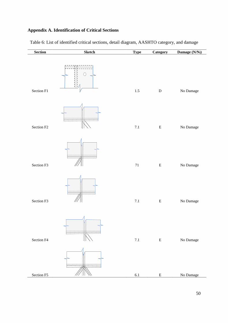
50
Appendix A. Identification of Critical Sections
Table 6: List of identified critical sections, detail diagram, AASHTO category, and damage
Section Sketch Type Category Damage (N/Nf)
Section F1
1.5 D No Damage
Section F2
7.1 E No Damage
Section F3
71 E No Damage
Section F3
7.1 E No Damage
Section F4
7.1 E No Damage
Section F5
6.1 E No Damage

51
Section F6
7.1 E No Damage
Section F6
7.1 E No Damage
Section F7 6.1 E 1.91032E-07
Section F8
6.1 E No Damage
Section F9
6.1 E 3.24412E-07
Section F10
6.1 E 1.06787E-05
Section F11
6.1 E 1.03828E-05
Section F12
7.1 E 9.1412E-06

52
Section F13
6.1 E 1.17139E-05
Section F14
6.1 E 1.15013E-05
Section F15
7.1 E 9.70907E-06
Section F16
7.1 E 8.57359E-07
Section F17
7.1 E 8.57359E-07
Section F18
5.3 C No Damage
Section F19
7.1 E No Damage
Section F20
6.1 E 1.02327E-05
Section F21
6.1 E 9.56954E-06

53
Section F22
7.1 E 7.11418E-06
Section F23
5.3 C No Damage
Section F24
7.1 E 1.37003E-06
Section Inside
Hole 1
1.5 D 8.95048E-07
Section Inside
Hole 2
1.5 D 5.0689E-07

54
Appendix B. Reservoir Cycle Counting Procedure
Cycle counting is used to get data from stress-time graph for fatigue analysis. There are two
methods for cycle counting: reservoir cycle counting and rain flow cycle counting. The
reservoir counting method was chosen because it was a better fit for the stress-time graphs from
the output data.
1. Shift part of the cycles so that the highest peaks are the starting point and ending point.
2. Imagine that the new graph is a reservoir filled with water.
3. Drain the reservoirs from the bottom of each valley.

55
a. Note the stress range from each drainage
b. Note the number of cycles per drainage. (Each valley is a cycle)
4. Create a table with the number of cycles at each stress range. No.
Cycles Stress Range [ksi]
3 10
1 30
2 20

56
Appendix C. Goodman Se Calculations
This section describes how to calculate the fatigue endurance limit (𝑆𝑒) using the Marin
Equation. The 5th edition of Mechanical Engineering Design describes the process used to
acquire the fatigue endurance limit (Shigley & Mischke, 1989). The Marin equation is shown
here as Equation 14.
𝑆𝑒 = 𝑘𝑎𝑘𝑏𝑘𝑐𝑘𝑑𝑘𝑓𝑆𝑒′ . Equation 14
The endurance limit, 𝑆𝑒′ , is based on results from a rotating beam specimen, and is calculated
using Equation 15.
𝑆𝑒′ = {
0.5 ∗ 𝑆𝑢𝑙𝑡 𝑆𝑢𝑙𝑡 ≤ 200 𝑘𝑠𝑖100 𝑘𝑠𝑖 𝑆𝑢𝑙𝑡 > 200 𝑘𝑠𝑖
Equation 15
Modification Factors
Surface factor 𝒌𝒂
Cracks often initiate at the surface of the material. The surface modification factor assesses the
quality of the finished surface along with the tensile strength of the material. Equation 16
calculates the factor 𝑘𝑎.
𝑘𝑎 = 𝑎𝑆𝑢𝑙𝑡𝑏 Equation 16
Table 7 determines the coefficients 𝑎 and 𝑏. The component is hot-rolled with corresponding
values for the coefficients determined from Table 7, and an ultimate strength of 𝑆𝑢𝑡 = 65 𝑘𝑠𝑖
for A572 steel. The surface factor is 𝑘𝑎 = 0.7189.
Table 7: Parameters for Marin surface modification factor
Surface Finish Factor a,
Sut given in ksi Exponent b
New Ground 1.43 -0.085
Machined or cold-drawn 2.7 -0.265
Hot-rolled 14.4 -0.718
As-forged 39.9 -0.995

57
Size factor 𝒌𝒃
The size factor is based on volume. The size factor for the rotating bar specimen is determined
by fitting a curve to experimental results. Volume affects the probability of failure as the
probability of stress interaction with a critical flaw increases as the volume increases decreasing
the endurance limit (Marin, 1962). Equation 17 calculates 𝑘𝑏 for members that are subjected
to bending and torsion.
𝑘𝑏 = {0.879𝑑−0.107
0.91𝑑−0.1570.11 ≤ 𝑑 ≤ 2 𝑖𝑛2 < 𝑑 ≤ 10 𝑖𝑛
Equation 17
There is no size effect for axial loading, therefore 𝑘𝑏 = 1. An effective diameter, 𝑑𝑒 is used in
place of 𝑑, in Equation 4, when the member is non-circular. The effective diameter 𝑑𝑒is
calculated in Equation 18.
𝑑𝑒 = 0.808√𝑏ℎ Equation 18
The variable 𝑏 is the base and ℎ is the height of the member’s cross-section. Equations for other
cross-sections are given in Mechanical Engineering Design, 5th Ed (Shigley & Mischke, 1989).
The component is under bending and has a rectangular cross-section. The variables 𝑏 = 10 𝑖𝑛
and ℎ =3
4𝑖𝑛, therefore the effective diameter is 𝑑𝑒 = 2.21 𝑖𝑛2. The size factor is 𝑘𝑏 = 0.803.
Load factor 𝒌𝒄
The way a component is loaded affects its fatigue strength. The load factor 𝑘𝑐 considers axial,
bending, or torsional loading, see Equation 19. Estimated values for 𝑘𝑐 are given below. The
component experiences bending therefore 𝑘𝑐 = 1.0.

58
𝑘𝑐 = {1.0
0.850.59
𝐵𝑒𝑛𝑑𝑖𝑛𝑔
𝐴𝑥𝑖𝑎𝑙𝑇𝑜𝑟𝑠𝑖𝑜𝑛
Equation 19
Temperature factor 𝒌𝒅
Surface temperature affects the endurance limit of the component because the ultimate
strength, 𝑆𝑢𝑡, varies with temperature. Higher temperatures cause the yield strength to decrease
leading to ductile failure. Lower temperatures can cause a brittle failure. Equation 20 calculates
the temperature factor.
𝑘𝑑 = 0.975 + 0.432(10−3)𝑇𝑓 − 0.115(10−5)𝑇𝐹2
+0.104(10−8)𝑇𝐹3 − 0.595(10−12)𝑇𝐹
4 Equation 20
The temperature variable, 𝑇𝐹 , is in Fahrenheit and within the range 70 ≤ 𝑇𝐹 ≤ 1000 ℉. The
temperature factor, at the average water temperature 𝑇𝐹 = 75℉ , is 𝑘𝑑 = 1.001.
Reliability factor 𝒌𝒆
As the percent of reliability increases the reliability factor 𝑘𝑒 decreases. Fatigue is based on the
number of cycles a component is subjected to and the S-N curves used to determine fatigue
endurance limits are based on statistical data. Figure 59 shows the uncertainty of the S-N curve
data leads to a mean strength value within a standard deviation in a normal distribution plot.
Reliability is the degree that a measurement, data, or calculation can be trusted. As reliability
increases the component failure area, illustrated in Figure 59, decreases and along with the
reliability factor. Table 8 gives percentages of reliability with the corresponding reliability
factor, 𝑘𝑒. A conservative estimate of 50% reliability was chosen for section 13, and the
reliability factor is, 𝑘𝑒 = 1.0.

59
Figure 59: Mean stress and strength curves
Table 8: Reliability factors corresponding to 8% standard deviation of the endurance limit
Reliability, % Reliability Factor, 𝑘𝑒
50 1.000
90 0.897
95 0.868
99 0.814
99.9 0.753
99.99 0.702
99.999 0.659
99.9999 0.620
Miscellaneous-Effects factor 𝒌𝒇
The miscellaneous-effects factor takes into consideration other environmental factors that can
affect the fatigue endurance limit. Miscellaneous-effects factor considers influences such as
corrosion, electrolytic plating, metal spraying, cyclic frequency, and frottage corrosion
(Shigley & Mischke, 1989). Since these values are environmentally dependent and hard to
determine the miscellaneous-effects factor is assumed to be 𝑘𝑓 = 1.0.
Calculating 𝑺𝒆
The endurance limit, 𝑆𝑒, is calculated for section 13. Assumptions were made about the type
of steel, temperature, reliability percentage, and other environmental factors to determine the
different factors. The cross-sectional area of section 13 was calculated to determine the size

60
factor. Section 13 is in bending and therefore the load factor coefficient chosen corresponds
with bending. Table 9 summarizes the different factors.
Table 9: Calculated Marin modification factors summary and modified endurance limit
Factor Value
𝑘𝑎 0.719
𝑘𝑏 0.803
𝑘𝑐 1.000
𝑘𝑑 0.999
𝑘𝑒 1.000
𝑘𝑓 1.000
𝑆𝑒′ 32.500 ksi
The calculated endurance limit, using Equation 21, is 𝑆𝑒 = 18.8 𝑘𝑠𝑖.
𝑆𝑒 = 𝑘𝑎𝑘𝑏𝑘𝑐𝑘𝑑𝑘𝑓𝑆𝑒′ . Equation 21

61
Appendix D. Friction Test Derivation
The coefficient of static friction between rusted steel and stainless steel is determined through
an experiment. The rusted steel is used as a ramp that the stainless-steel block slides down. The
test consists of raising the ramp until the stainless piece begins to move. Once the stainless-
steel block begins to move the gravity force on the block overcomes the friction force, see
Figure 60 b. Figure 60 demonstrates how the ramp experiment allows for the static friction of
coefficient to be calculated. Figure 33 in Section 8.1 shows the two steel blocks used for the
test (non-corroded and corroded) and the stainless-steel ramp.
Figure 60: Static friction of coefficient test and derivation

62
Appendix E. Friction Clamp Calculations
The friction force is calculated using a free body diagram (Figure 61), a known static coefficient
of friction (μ), and a known pre-stress force (𝐹𝑝𝑟𝑒). There are two planes of friction, as seen in
Figure 56. The two planes of friction divide the required clamping force (𝑁) in half. The static
coefficient of friction derived in Appendix D is 𝜇 = 0.34. The previously derived pre-stress,
Section 8, force is 𝐹𝑝𝑟𝑒 = 366.57 𝑘𝑖𝑝𝑠 The calculated downward force is 𝑁 = 540 𝑘𝑖𝑝𝑠, see
Figure 61.
Figure 61: Free body diagram of friction clamp and derivation

63
Appendix F. Cycle Estimation for Experimental Test
The estimated number of cycles to reach damage is determined using AASHTO chapter 6.
Table 6.6.1.2.3-1 from AASHTO chapter 6 gives the category, constant (𝐴 ) (ksi3), and
threshold (∆𝐹𝑇𝐻) (ksi). The stress range (∆𝐹𝑁) is determined from the gate model max-in-plane
stress data. Equation 22, from AASHTO chapter 6 equation 6.6.1.2.5-2, is used to calculate the
number of cycles to damage at the given stress range.
𝑁 =𝐴
∆𝐹𝑁3 Equation 22
At the stress range ∆𝐹 = 24.467 𝑘𝑠𝑖 , calculated from the gate model, the number of cycles
is 𝑁 = 73,468. Due to the capability of the hydraulic actuator the tensile force applied during
testing is 50 kips. The area the load is applied to is 𝐴𝑎𝑟𝑒𝑎 = 12.5 𝑖𝑛2. At the tensile load of
𝑃 = 50 𝑘𝑖𝑝𝑠 and 𝐴𝑎𝑟𝑒𝑎 = 12.5 𝑖𝑛2 the stress ∆𝐹 = 4 𝑘𝑠𝑖. The number of cycles to damage at
∆𝐹 = 4 𝑘𝑠𝑖 is 𝑁 = 17.2 ∗ 106.