Did U.S. Politicians Expect the China Shock?

Matilde Bombardini, Bingjing Li

and Francesco Trebbi*

January 2021

Abstract

In the two decades straddling China’s WTO accession, the China Shock, i.e. the rapidtrade integration of China in the early 2000s, has had a profound economic impact acrossU.S. regions. It is now both an internationally litigated issue and the casus belli for a globaltrade war. Were its consequences unexpected? Did U.S. politicians have imperfect informa-tion about the extent of China Shock’s repercussions in their district at the time when theyvoted on China’s Normal Trade Relations status? Or did they have accurate expectations,yet placed a relatively low weight on the subconstituencies that ended up being adverselyaffected? Information sets, expectations, and preferences of politicians are fundamental, butunobserved determinants of their policy choices. We apply a moment inequality approachdesigned to deliver unbiased estimates under weak informational assumptions on the informa-tion sets of members of Congress. This methodology offers a robust way to test hypothesesabout the expectations of politicians at the time of their vote. Employing repeated rollcall votes in the U.S. House of Representatives on China’s Normal Trade Relations status,we formally test what information politicians had at the time of their decision and con-sistently estimate the weights that constituent interests, ideology, and other factors had incongressional votes. We show how assuming perfect foresight of the shocks biases the roleof constituent interests and how standard proxies to modeling politician’s expectations biasthe estimation. We cannot reject that politicians could predict the initial China Shock inthe early 1990s, but not around 2000, when China started entering new sectors, and find amoderate role of constituent interests, compared to ideology. Overall, U.S. legislators appearto have had accurate information on the China Shock, but did not place substantial weighton its adverse consequences.

* Bombardini: UC Berkeley Haas School of Business, CEPR and NBER; Li: National University ofSingapore; Trebbi: UC Berkeley Haas School of Business, CEPR and NBER. We would like to thankBen Faber, Gordon Hanson, Andres Rodriguez-Clare, Gerard Roland, Peter Schott, and seminarparticipants at UC Berkeley, Johns Hopkins, NBER ITI Fall 2020 Meeting, Shanghai University ofFinance and Economics Summer Trade Workshop, the Federal Reserve Board of Governors, the U.S.Census Bureau, and Yale University for their comments and discussion. Leopoldo Gutierre providedexcellent research assistance.

1 Introduction

The China Shock, the large surge in imports from China that started in the 1990s and that has

turned China into one of the U.S. main trading partners, has received broad attention in academia

and policy making. Although early research by Autor et al. (2013, 2016) and Pierce and Schott

(2016) focused mainly of its employment effects, a large literature has expanded the analysis to

health, social, and political consequences of the shock.1 While in hindsight China’s entry in the

U.S. market may seem like a preordained outcome, in a series of roll call votes during the 1990s

members of Congress were faced with the choice of allowing China to maintain its Normal Trade

Relations (NTR), and ultimately obtain Permanent NTR, status.

In this paper we ask to what degree U.S. politicians were informed about the consequences of

the China Shock for their voters and how much the expected impact on their constituents affected

their support in favor or against China’s NTR status.2 These two questions are intrinsically related

and point to the difficulty of modeling forward-looking expectations and decisions by policy makers

in a context where these choices depend on consequences that are not known at the time of the

vote. We present a model and an estimation strategy of the decisions and expectations of law

makers. In this, we depart from the empirical political economy literature on legislative voting

(Poole and Rosenthal, 1997; Heckman and Snyder, 1997; Clinton et al., 2004; Canen et al., 2020)

and extend it in a distinct direction, as a formal analysis of law makers’ information sets and

expectations does not typically figure in standard empirical models of voting.

To provide intuition, consider the following. A naıve approach to estimating the importance of

constituent interests may be the replacement of the politician’s expectations of the China Shock

with their realized values. However, assuming that politicians are perfectly informed about future

shocks when they are not, necessarily implies a downward bias in the coefficient that measures the

preference weight placed on constituent interests within a discrete choice voting model. This is

due to an intuitive error-in-variables argument (i.e. the mechanical negative covariance between

the expectational error and the realized future value of the shock). Without correction, a small

coefficient may be interpreted as low responsiveness of politicians to subconstituents’ fortunes,

possibly indicating a political accountability problem (Kalt and Zupan, 1984, 1990). In reality, a

small coefficient may be as well the result of assuming that politicians are better informed than

they truly are. Yet, this rather points to a limited expertise or insufficient information acquisition

of legislators (Krehbiel, 1992). Because these interpretations have distinct policy implications and

1Among the others, see Greenland and Lopresti (2016), Feler and Senses (2017), Autor et al. (2019), Greenlandet al. (2019), Autor et al. (2019) and Autor et al. (2020a).

2The role of electoral constituencies and subconstituencies in driving the behavior of members of Congress hasplayed a central role in the analysis of policy support in Washington at least since Fenno (1978); Peltzman (1984).See also Mian et al. (2010, 2014) for more recent applications.

1

they call for different remedies, it seems relevant to be able to distinguish between them.

To address the estimation challenge, we link the political economy literature to a separate

strand of the international trade literature. The novel moment inequality methodology of Dickstein

and Morales (2018), developed in the context of the decision of firms to export to foreign markets,

allows us to consistently operate within an expectational environment where what belongs to the

information set of the decision maker is only partially observed. That is, this moment inequality

approach only requires the econometrician to know a subset of the information available to the

politician at the time of his or her vote for consistent estimation of parameters – a much less

demanding restriction. This approach turns out to be particularly informative in our context. It

allows us to estimate a voting model under general assumptions about the politician’s information

set and expectations, and therefore to answer the question of how much politicians cared about

the China Shock in the first place.

Naturally, economic consequences on their voters were not the only considerations affecting

individual law makers’ support for NTR and our model accommodates these features.3 It is

generally believed that several members of Congress voted to withhold NTR status in order to

affect China’s position on human rights, as the series of yearly roll call votes on China’s NTR

status between 1990 and 2001 started after the Tiananmen Square events of 1989. We therefore

also allow the voting behavior to depend on the ideological position of the legislator and the

expected electoral cost of supporting China’s NTR status, taking into consideration the district-

specific impact of China’s continued and growing exports to the U.S.. Further, in the utility

function, ideology also captures the position of the legislator towards free trade policy, that is the

value the politician places on the collective gains from maintaining low import tariffs.

We establish two main results. The first result is a moderate role of constituent interests. An

interquartile difference in the value of the the shock decreases the probability of voting in favor

of NTR for China by roughly 3-5 percentage points, while an analogous difference in ideology

creates a 13-17 percentage point increase in the probability of supporting NTR for China. In

our heterogeneity analysis, we show that constituent interests are more important for Democrats

than for Republicans, and for politicians that were elected with small vote margins (a margin of

responsiveness supported by other studies, see discussion in Mian et al. 2010; Ladewig 2010).

The second main result of our analysis is that politicians possessed a significant amount of

knowledge about the future China Shock. In some years we cannot reject that they perfectly

forecasted the shock that would hit their district in the next five years. More precisely, for all

years from 1990 to 2001 we cannot reject that politicians had, at least, enough information to

3There is a vast literature discussing pure economic models of voting where electoral constituents (Peltzman,1984) or subconstitutents matter for roll call voting in Congress versus ideology of members of Congress (Kalt andZupan, 1984, 1990; Levitt, 1996). For a recent review see (Mian et al., 2014).

2

forecast 55 percent of the variation in the China Shock. Perhaps surprisingly, our findings imply

that knowledge decreases over the 1990s, a result that is plausible given that China’s comparative

advantage shifted substantially during the late 1990s and early 2000s. Comparing legislators across

parties, we find that Democrats were systematically more informed than Republicans, with the

exception of the early 1990s, a period when they are both equally informed. We also present several

validation exercises for our approach, including a comparison of the NTR voting for China to the

NTR voting for the case of Vietnam, showing how the moment inequality estimation highlights

similar patterns in terms of information sets and preferences for comparable votes. Our findings

on the extent of the information sets of U.S. politicians (and their fairly accurate expectations)

appear in line with the extent of information inferred from stock price responses around the China

permanent NTR vote (e.g. Greenland et al., 2020).

Finally, we employ the estimated model to perform counterfactual exercises in which we give

politicians perfect information about the upcoming shocks and calculate the change in voting

behavior that would have resulted from the additional information. We find that overall support for

China’s NTR status would not have changed substantially in the presence of perfect information.

In essence, to the question in the title “Did U.S. politicians expect the China Shock?” our

answer is “Yes, but they did not give it substantial weight.” Counterfactual simulations in section

6.2, where such weight is increased for all lawmakers in our sample for given baseline information,

show that pro-China legislation would have been overturned.

One important premise to the question we are posing is the assumption that the electorate is

generally attuned to trade policy positions of their representatives. It would otherwise be unclear

why politicians would care about the reaction of voters. While it is implausible to assume that

voters have a complete command of specific trade policy measures, a number of papers have docu-

mented the impact of the China shock and the recent trade war on electoral outcomes. Autor et al.

(2020b) find that districts more affected by the China shock saw an increase in Fox News viewer-

ship and elected more conservative Republicans and, to a lesser extent, more liberal Democrats,

thus inducing more polarization.4 Another recent contribution by Che et al. (2020) finds that

the 2010’s reaction to the China shock is due to the anti-trade turn taken by the Republican

party after the appearance of the Tea Party. The same paper finds that, during the 2000s, the

areas affected by the China shock voted more in favor of Democrats. Blanchard et al. (2019) also

document a significant electoral impact of the trade war on the vote share of Republicans in 2018.

Interestingly, the negative effect on GOP vote share coming from retaliatory tariffs imposed by

U.S. trading partners is not mirrored by a positive effect due to the protection offered by import

tariffs. In sum, these recent papers offer a clear justification for making constituent interests a

major component of the decision to vote on an important trade policy measure, like maintaining

4Colantone and Stanig (2018) document a similar result for Western European countries.

3

and expanding China’s Normal Trade Relations status.5

This paper contributes directly to the literature on Congressional voting, in particular on trade

policy. An example is Baldwin and Magee (2000), which estimates the importance of constituent

interests and campaign contributions from business and labor groups in three trade bill votes in the

1990s. Relative to Baldwin and Magee (2000), we sharpen the estimation of the role of constituent

interests by employing a more precise measure of how constituents were impacted by the policy, but

mostly by applying a new econometric methodology to expectations of politicians. A more recent

paper by Feigenbaum and Hall (2015) studies the impact of the China Shock on congressional

voting on trade bills in general and finds that congressmen in districts more negatively affected are

less likely to vote in favor of trade promoting bills, as classified by the Cato Institute, a think-tank

in Washington DC. Differently from Feigenbaum and Hall (2015)’s retrospective view, we take a

prospective angle in modeling voting behavior, where law makers are deciding to vote based on the

future electoral consequences of their decision. In the broader literature on the political economy

of trade policy, Rodrik (1995) offers a more conceptual framework and depicts trade policy as

emerging from demand (interest groups, grassroots, etc) and supply (government) factors. This

paper’s contribution sheds light on the individual behavior of legislators that constitutes a crucial

element of the policy “supply side”.

Beyond the trade policy literature, this paper speaks to the established empirical literature

focused on modeling voting in legislatures. The elements of this vast scholarship that are closer

to our paper span political economy and political science (Poole and Rosenthal, 1984; Levitt,

1996; Heckman and Snyder, 1997; Poole and Rosenthal, 1997; Jenkins, 2000; Clinton et al., 2004;

McCarty et al., 2006; Canen et al., 2020). Modeling prospective behavior of legislators does

figure in this strand of research, as it is often postulated that a representative politician acts

by “determining her roll-call vote choice based on which legislative options will maximize her

future utility” (Ladewig, 2010). Stimson et al. (1995) argue that in congressional voting “elected

politicians. . . sense the mood of the moment, assess its trends, and anticipate its consequences for

future elections”. However, expectations and information sets of lawmakers are rarely explicitly

modeled as part of the empirical approach. The more complex exercise of assessing whether a

politician may not be responding to prospective constituent conditions in her or his vote because

of limited information or because of policy preferences appears unexplored. We contribute to this

by showing how this moment inequality approach provides a useful stepping stone in estimating

prospective behavior of law makers.

Less directly, our application offers an alternative and complementary view to the empirical

5A recent paper by Fajgelbaum et al. (2020) points to the importance of constituent interests in the structureof tariffs in the Trade War the US started in 2018. U.S. import tariffs are such that marginal counties (those witha Republican vote share of around 50 percent) receive the highest level of protection.

4

literature focused on modeling the expectations of policy makers. This analysis has traditionally

found important applications in Macroeconomics (Primiceri, 2006; Sargent et al., 2006), and in

this sense, the paper connects to a broader set of questions than congressional voting alone. Our

estimates also speak to the modeling of government preferences, a key area of political economy.6

The rest of the paper proceeds as follows. Section 2 builds a baseline model of probabilistic

voting useful for rationalizing the data. Section 3 lays out the estimation methodology including

appropriate model specification tests, while section 4 describes the data on roll call votes and the

China Shock. Section 5 reports estimation results and the following section presents counterfactual

analysis based on our baseline estimates. Section 7 concludes.

2 Empirical model

This section presents a simple model of probabilistic voting for members of Congress. Indicate a

congressional cycle with t = 1, 2, ...., T . Each period a single bill focused on a main policy issue is

introduced – in this application maintaining Normal Trade Relations with China. As previously

discussed, such bills were typically presented to the U.S. legislative branch and voted upon once

per congressional cycle, so that t may equivalently indicate time and bill number.

Let us indicate with xt ∈ R a policy position favorable to trade normalization, so that a

Yes vote will indicate a vote for xt. Consequently, one interprets a No vote as a vote against

normal trade relations, qt ∈ R. This notation allows for the two positions to be affected by some

nuance over time and neither position is assumed to be exactly constant in time. In the empirical

analysis we will simply make sure that a Yes vote will be consistently labeled to the support for

the alternative xt.

Indicate by i = 1, ..., N individual legislators, where N is large.7 We will assume that individ-

ual i’s preferences are described by a random utility framework. We also posit a spatial voting

environment for the members of Congress. Spatial voting is a successful and informative modeling

approach to the description of congressional behavior and it has found substantial support in the

literature (Poole and Rosenthal 1997; Heckman and Snyder 1997; Clinton et al. 2004; McCarty

et al. 2006; Bateman et al. 2017).

For simplicity of exposition (relaxed in the empirical application later), the deterministic com-

ponent of the politician’s utility is assumed to depend on: (i) the distance of the bill from his/her

ideological position θi; (ii) an electoral motive, summarized by his/her expected future electoral

support Vi,t+1 (for example, due to the employment consequences of i’s voting behavior from the

6For early applications, see Alesina (1988); Alesina and Tabellini (1990); Drazen and Masson (1994).7What follows can be applied to each chamber independently at the cost of omitting interactions between the

two chambers, such as resolutions and conferences. N = 435 for the House and N = 100 for the Senate.

5

perspective of his/her constituents).

Concerning (i), political ideology θi ∈ R is a unidimensional and fixed characteristic of i. The

assumption of unidimensionality is appropriate in the time period under analysis (see McCarty

et al. 2006). The assumption of constant policy preferences has been validated repeatedly in the

literature on Congress (Moskowitz et al. 2017 for a discussion). We use the ideological positions

θi from DW-Nominate first dimension scores (Poole and Rosenthal, 1997).8 This follows a com-

mon approach in modeling congressional voting when the explicit estimation of such preference

parameters is peripheral to the main empirical analysis like in this case (e.g., Mian et al. 2010,

2014).9

Concerning (ii), let us indicate by Si,t a proxy for the degree of exposure of the local labor

market in the district represented by i at time t to increasing imports from China (the China

Shock as presented in Autor et al. 2016). Assume the potential electoral impact of the China

Shock in the district represented by politician i at time t+ 1 is defined by:

Vi,t+1 = ht(di,t, Si,t+1) + ei,t+1,

where di,t is the voting decision made by the politician, and

E [ei,t+1|di,t, Si,t+1, Ii,t] = 0

ht(di,t, Si,t+1) = γ0t + γ1

t Si,t+1×1 di,t = vote forxt (1)

+γ2t Si,t+1 × 1 di,t = vote for qt

= γ0t + γ2

t Si,t+1 +(γ1t − γ2

t

)Si,t+1 × 1 di,t = vote forxt

where 1 . is an indicator function and Ii,t is the information set of politician i at t. Note that the

function ht(.) introduces both a direct effect of the China Shock on electoral support independently

of i’s vote and a component that depends on the interpretation by the voters of their representative

i’s decision. These electoral effects are allowed to vary over time. Note further that we introduce

the China Shock directly in the electoral outcome for politician i, but such effect can be interpreted

as the composite of two forces: the impact of the shock on employment outcomes and the impact

of employment outcomes on electoral results.10

8For further reference, see www.voteview.com9The reader interested in the estimation of θi can find a detailed analysis in Canen et al. (2020) and references

therein. Due to lack of sample overlap the Canen et al. (2020) estimates cannot be used in our application.10When considering the economic effects of trade with China, it may be natural to consider the role of exports,

and not only imports. Recent work by Feenstra et al. (2019) shows that the exports-led increase in the demandfor labor has almost matched the negative employment effects of the China Shock. An important observation inthis regard is that Feenstra et al. (2019) consider U.S. exports not only to China, but to all its trading partners.When considering only China as a destination market, exports and export growth were markedly smaller and didnot have as large a positive effect on employment, as initially shown in Autor et al. (2013). Since NTR votes did

6

The expected utility for a politician i of taking decision dt, given information set Ii,t is:

U(ξi,t, di,t; θi, Ii,t)

= u (‖ di,t − θi ‖) + δE [Vi,t+1|di,t, Ii,t] +

ξi,t,x if di,t = vote forxt

ξi,t,q if di,t = vote for qt,

where u (‖ . ‖) indicates an ideological loss that is function of the distance of the policy from the

ideal point of i. The term Vi,t+1 indicates the future electoral outcome for the district represented

by i. We assume a quadratic loss function u(.) and i.i.d. Gaussian term ξi,t,d ∼ N(0, σ2ξ ). This

implies the useful convolution ξi,t = ξi,t,q−ξi,t,x ∼ N(0, 2σ2ξ ). A standard identification requirement

in discrete choice problems with Gaussian shocks (e.g. in probit) further requires the normalization

2σ2ξ = 1, which we impose.

We define the variable Yi,t as an indicator function that is equal to 1 when legislator i decides

to vote Yes on xt and 0 when the legislator votes in favor of qt :

Yi,t = 1U(ξi,t, xt; θi, Ii,t) > U(ξi,t, qt; θi, Ii,t) (2)

= 1

−1

2

((xt − θi)2 − (qt − θi)2)+ δ (E [Vi,t+1|xt, Ii,t]− E [Vi,t+1|qt, Ii,t]) ≥ ξit

.

We can write the probability of Yi,t = 1 as:

Pr(Yi,t = 1|Ii ,t)

= Φ

(−1

2

((xt − θi)2 − (qt − θi)2)

+δ (E [Vi,t+1|xt, Ii,t]− E [Vi,t+1|qt, Ii,t])

), (3)

where Φ is the standard normal cumulative density function and E [Vi,t+1|xt, Ii,t]−E [Vi,t+1|qt, Ii,t] is

the expected net loss (or net gain) of electoral support due to the China Shock in the constituency

represented by politician i in the future electoral cycle, given the information available to i at

t. This implies that the probability of voting Yes depends on the expectations of the electoral

consequences of voting Yes relative to voting No, which are unobserved by the econometrician.

The higher is the expected electoral gain of voting Yes, the higher the likelihood of voting Yes.

It follows from (1) that:

E [Vi,t+1|xt, Ii,t]− E [Vi,t+1|qt, Ii,t] =(γ1t − γ2

t

)E [Si,t+1|Ii,t] .

Setting δt = δ (γ1t − γ2

t ) and simplifying the relative loss function −12

((xt − θi)2 − (qt − θi)2) as

not have obvious implications for the U.S. worldwide export prospects, we exclude exports from our main analysisof voting decisions, but include them in a robustness sectin in Appendix E.4.

7

atθi + bt, where at = xt − qt and bt = 12(q2t − x2

t ), we can further rewrite (2) and (3), respectively,

as:

Yi,t = 1atθi + bt + δtE [Si,t+1|Ii,t] ≥ ξi,t, (4)

Pr(Yi,t = 1|Ii,t) = Φ (atθi + bt + δtE [Si,t+1|Ii,t]) . (5)

A key parameter is δt, which gauges the weight in the politician’s vote choice of his/her expectations

about the future China Shock, E [Si,t+1|Ii,t]. We discuss two distinct approaches to the estimation

of this and the other parameters in the next section.

3 Expectations and information set of politicians: Esti-

mation

A key contribution of this paper is the analysis of the information set available to politicians to

forecast the labor market effects of the China Shock at the time of a roll call vote. There are two

fundamentally different approaches, which in turn hinge on the answer to the following question:

is the politician’s information set Ii,t known to the econometrician? When the answer is in the

affirmative, then estimation can be performed by maximum likelihood or method of moments.

When the econometrician knows only a subset of the information available to politicians, then one

can adopt a moment inequality estimator. We discuss these two approaches in turn, but we first

start with describing the three benchmark information sets that we will consider throughout the

paper:

(i) Minimal Information: the politician knows his own ideological position θi, but the only infor-

mation a politician has about the economic impact of the China Shock is the current share

of population employed in manufacturing in district i, ShareMfgi,t;

(ii) Baseline Information: the politician has access to the minimal information set, plus the

current period China Shock Si,t;

(iii) Perfect Foresight: the politician has perfect foresight of the labor market consequences of

the China Shock, so that E [Si,t+1|Ii,t] = Si,t+1.

3.1 Politician’s information set fully known to the econometrician:

MLE

When the econometrician knows the content of the politician’s information set, then the parameter

vector ωt = at, bt, δt can be estimated by maximum likelihood for each cycle. Based on expression

8

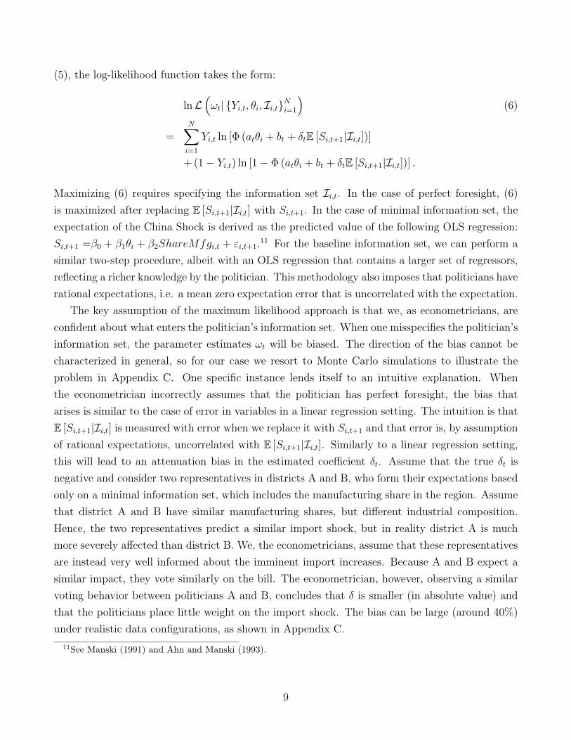
(5), the log-likelihood function takes the form:

lnL(ωt| Yi,t, θi, Ii,tNi=1

)(6)

=N∑i=1

Yi,t ln [Φ (atθi + bt + δtE [Si,t+1|Ii,t])]

+ (1− Yi,t) ln [1− Φ (atθi + bt + δtE [Si,t+1|Ii,t])] .

Maximizing (6) requires specifying the information set Ii,t. In the case of perfect foresight, (6)

is maximized after replacing E [Si,t+1|Ii,t] with Si,t+1. In the case of minimal information set, the

expectation of the China Shock is derived as the predicted value of the following OLS regression:

Si,t+1 =β0 + β1θi + β2ShareMfgi,t + εi,t+1.11 For the baseline information set, we can perform a

similar two-step procedure, albeit with an OLS regression that contains a larger set of regressors,

reflecting a richer knowledge by the politician. This methodology also imposes that politicians have

rational expectations, i.e. a mean zero expectation error that is uncorrelated with the expectation.

The key assumption of the maximum likelihood approach is that we, as econometricians, are

confident about what enters the politician’s information set. When one misspecifies the politician’s

information set, the parameter estimates ωt will be biased. The direction of the bias cannot be

characterized in general, so for our case we resort to Monte Carlo simulations to illustrate the

problem in Appendix C. One specific instance lends itself to an intuitive explanation. When

the econometrician incorrectly assumes that the politician has perfect foresight, the bias that

arises is similar to the case of error in variables in a linear regression setting. The intuition is that

E [Si,t+1|Ii,t] is measured with error when we replace it with Si,t+1 and that error is, by assumption

of rational expectations, uncorrelated with E [Si,t+1|Ii,t]. Similarly to a linear regression setting,

this will lead to an attenuation bias in the estimated coefficient δt. Assume that the true δt is

negative and consider two representatives in districts A and B, who form their expectations based

only on a minimal information set, which includes the manufacturing share in the region. Assume

that district A and B have similar manufacturing shares, but different industrial composition.

Hence, the two representatives predict a similar import shock, but in reality district A is much

more severely affected than district B. We, the econometricians, assume that these representatives

are instead very well informed about the imminent import increases. Because A and B expect a

similar impact, they vote similarly on the bill. The econometrician, however, observing a similar

voting behavior between politicians A and B, concludes that δ is smaller (in absolute value) and

that the politicians place little weight on the import shock. The bias can be large (around 40%)

under realistic data configurations, as shown in Appendix C.

11See Manski (1991) and Ahn and Manski (1993).

9

3.2 Politician’s information set partially known to the econometrician:

Moment inequality approach

In the previous section we have shown that the maximum likelihood approach relies on an accurate

knowledge by the econometrician of the information set possessed by the politician. The alternative

estimation method proposed by Dickstein and Morales (2018), based on moment inequalities,

does not require full knowledge of Ii,t, but rather of a subset of variables Zi,t ⊆ Ii,t. That

is, the politician may know more than Zi,t in forming his/her forecast, but she knows at least

the covariates Zi,t. Assuming only partial knowledge of Ii,t comes at the cost of less precise

identification. We will not be able to point identify the elements of the parameter vector ωt,

but only to set identify them. Whether these sets are sufficiently tight to be informative will be

carefully discussed in the results section.

The second important goal of our analysis is to ascertain the extent of the information set

of legislators. This, in turn, involves a formal analysis of which subset of variables a politician

considers at the time of his/her vote through an application of specification selection tests proposed

by Bugni et al. (2015). Being able to reject that certain variables are used in the politician’s forecast

allows us to learn about the process of decision making of legislators in this particular setting:

what they knew and considered relevant at the time of their vote. In this exercise the voting

model and data are kept constant, but the subset of variables assumed part of the information set

is varied.

We will allow politicians to have time varying information sets and we will formally test whether

certain groups of legislators have identical information sets or not. For instance, we assess whether

members of higher levels of chamber seniority have broader information sets than lower seniority

members, or whether members of opposing parties share the same information set. Questions of

asymmetry of information sets across party lines are increasingly common in the political economy

literature focused on polarization12 and our application offers a formal approach to this problem

for members of Congress.

A final question that the approach allows us to answer is whether, had politicians had a more

complete information set, their votes for trade normalization with China would have been different.

These counterfactuals are simulated within the same structure of expectations and information

we just described.

Throughout, we maintain the assumption of rational expectations on the part of politicians,

that is the expectational error εi,t+1 = Si,t+1 − E [Si,t+1|Ii,t] has mean zero, E [εi,t+1|Ii,t] = 0

and is uncorrelated with E [Si,t+1|Ii,t]. This means that politicians do not systematically skew

their prediction or ignore elements of their information set which would systematically help in

12See Alesina et al. (2020).

10

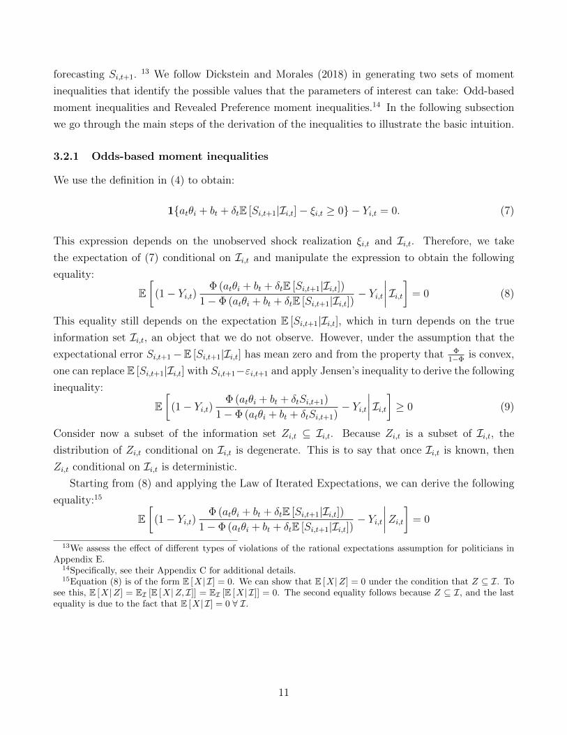
forecasting Si,t+1.13 We follow Dickstein and Morales (2018) in generating two sets of moment

inequalities that identify the possible values that the parameters of interest can take: Odd-based

moment inequalities and Revealed Preference moment inequalities.14 In the following subsection

we go through the main steps of the derivation of the inequalities to illustrate the basic intuition.

3.2.1 Odds-based moment inequalities

We use the definition in (4) to obtain:

1atθi + bt + δtE [Si,t+1|Ii,t]− ξi,t ≥ 0 − Yi,t = 0. (7)

This expression depends on the unobserved shock realization ξi,t and Ii,t. Therefore, we take

the expectation of (7) conditional on Ii,t and manipulate the expression to obtain the following

equality:

E[

(1− Yi,t)Φ (atθi + bt + δtE [Si,t+1|Ii,t])

1− Φ (atθi + bt + δtE [Si,t+1|Ii,t])− Yi,t

∣∣∣∣ Ii,t] = 0 (8)

This equality still depends on the expectation E [Si,t+1|Ii,t], which in turn depends on the true

information set Ii,t, an object that we do not observe. However, under the assumption that the

expectational error Si,t+1−E [Si,t+1|Ii,t] has mean zero and from the property that Φ1−Φ

is convex,

one can replace E [Si,t+1|Ii,t] with Si,t+1−εi,t+1 and apply Jensen’s inequality to derive the following

inequality:

E[

(1− Yi,t)Φ (atθi + bt + δtSi,t+1)

1− Φ (atθi + bt + δtSi,t+1)− Yi,t

∣∣∣∣ Ii,t] ≥ 0 (9)

Consider now a subset of the information set Zi,t ⊆ Ii,t. Because Zi,t is a subset of Ii,t, the

distribution of Zi,t conditional on Ii,t is degenerate. This is to say that once Ii,t is known, then

Zi,t conditional on Ii,t is deterministic.

Starting from (8) and applying the Law of Iterated Expectations, we can derive the following

equality:15

E[

(1− Yi,t)Φ (atθi + bt + δtE [Si,t+1|Ii,t])

1− Φ (atθi + bt + δtE [Si,t+1|Ii,t])− Yi,t

∣∣∣∣Zi,t] = 0

13We assess the effect of different types of violations of the rational expectations assumption for politicians inAppendix E.

14Specifically, see their Appendix C for additional details.15Equation (8) is of the form E [X| I] = 0. We can show that E [X|Z] = 0 under the condition that Z ⊆ I. To

see this, E [X|Z] = EI [E [X|Z, I]] = EI [E [X| I]] = 0. The second equality follows because Z ⊆ I, and the lastequality is due to the fact that E [X| I] = 0 ∀ I.

11

which, by the same arguments employed to obtain (9), yields the inequality:

E[mobl

∣∣Zi,t] ≥ 0 (10)

mobl = (1− Yi,t)

Φ (atθi + bt + δtSi,t+1)

1− Φ (atθi + bt + δtSi,t+1)− Yi,t

Notice that (10) is increasing in δt, so this condition identifies a lower bound for this parameter.

We use the subscripts l, u to indicate the lower bound and upper bound inequalities.

Following a similar logic, one can derive a moment condition that further bounds the parame-

ters of interest ωt:

E[mobu

∣∣Zi,t] ≥ 0 (11)

mobu = Yi,t

1− Φ (atθi + bt + δtSi,t+1)

Φ (atθi + bt + δtSi,t+1)− (1− Yi,t)

Notice that mobu is decreasing in δt and therefore moment inequality (11) identifies an upper bound

for this parameter.

3.2.2 Revealed preference moment inequalities

The second set of moment inequalities derives from the revealed preference argument that a

politician will vote Yes if and only if the benefit from doing so is positive, hence:

Yi,t (atθi + bt + δtE [Si,t+1|Ii,t]− ξi,t) ≥ 0 (12)

Because, again, ξi,t is unobserved, we take the expectation of (12), conditional on θi and Ii,t and

obtain the following inequality:

E [Yi,t (atθi + bt + δtE [Si,t+1|Ii,t]) + Γi,t| Ii,t] ≥ 0 (13)

where Γi,t = −E [Yi,tξi,t| Ii,t] = (1− Yi,t) φ(atθi+bt+δtE[Si,t+1|Ii,t])1−Φ(atθi+bt+δtE[Si,t+1|Ii,t]) , and φ is the standard normal

probability density function. Once again the expression in inequality (13) contains the unobserved

expectation E [Si,t+1|Ii,t]. Because φ1−Φ

is convex, we can apply the same logic as for equation (9).

The resulting inequality will be weaker than (13) and is given by:

E [mrpl |Zi,t] ≥ 0 (14)

mrpl = Yi,t (atθi + bt + δtSi,t+1) + (1− Yi,t)

φ (atθi + bt + δtSi,t+1)

1− Φ (atθi + bt + δtSi,t+1)

12

Starting from another revealed preference inequality:

(1− Yi,t) (ξi,t − atθi − bt − δtE [Si,t+1|Ii,t]) ≥ 0,

we can obtain a second revealed-preference moment inequality in a similar manner:

E [mrpu |Zi,t] ≥ 0 (15)

mrpu = − (1− Yi,t) (atθi + bt + δtSi,t+1) + Yi,t

φ (atθi + bt + δtSi,t+1)

Φ (atθi + bt + δtSi,t+1).

The moment inequalities defined by (10), (11), (14) and (15) are conditional on values of the vectors

Zi,t, which we allow to contain different variables, characterizing different possible information

sets possessed by politicians. The following theorem indicates that the true parameter vector

ωt = at, bt, δt is contained in the set of parameters that are in compliance with the odds-based

and revealed preference moment inequalities. Hence, the parameters of interest are partially

identified:16

Theorem 1. (Dickstein and Morales, 2018) At the true value of the parameter vector ωt =

at, bt, δt the following four moment inequalities are satisfied:

E[mobu

∣∣Zi,t] ≥ 0

E[mobl

∣∣Zi,t] ≥ 0

E [mrpu |Zi,t] ≥ 0

E [mrpl |Zi,t] ≥ 0

where Zi,t is the set of variables known by politician i at time t.

3.3 Estimation implementation

In this section we lay out the steps to construct confidence sets for the parameters of interest

at, bt, δt. Conditional moments (10), (11), (14) and (15) cannot be directly employed for empir-

ical applications because conditioning on each possible value of Zi,t is computationally unfeasible.

The standard solution in the moment inequality literature, which we adopt, is to transform con-

ditional into unconditional moment inequalities, which can be directly employed in estimation.17

This is not innocuous in that information is lost in transitioning from conditional inequalities

16See Appendix C in Dickstein and Morales (2018) for the proof of this result.17Starting from a moment inequality of the form E[m|Z] ≥ 0, let us consider an instrument function g (Z) > 0.

Multiplying the two and taking expectation yields E [g (Z)E[m|Z]] ≥ 0 which implies E [g (Z)m] ≥ 0 wheneverg (Z) is Z-measurable.

13

to a relatively smaller set of unconditional inequalities. As a result, the parameters that satisfy

conditional moment inequalities may be a small subset of those that satisfy the unconditional

moments. Whether these larger confidence sets remain sufficiently informative is again an issue

to be reckoned with once we discuss our results.

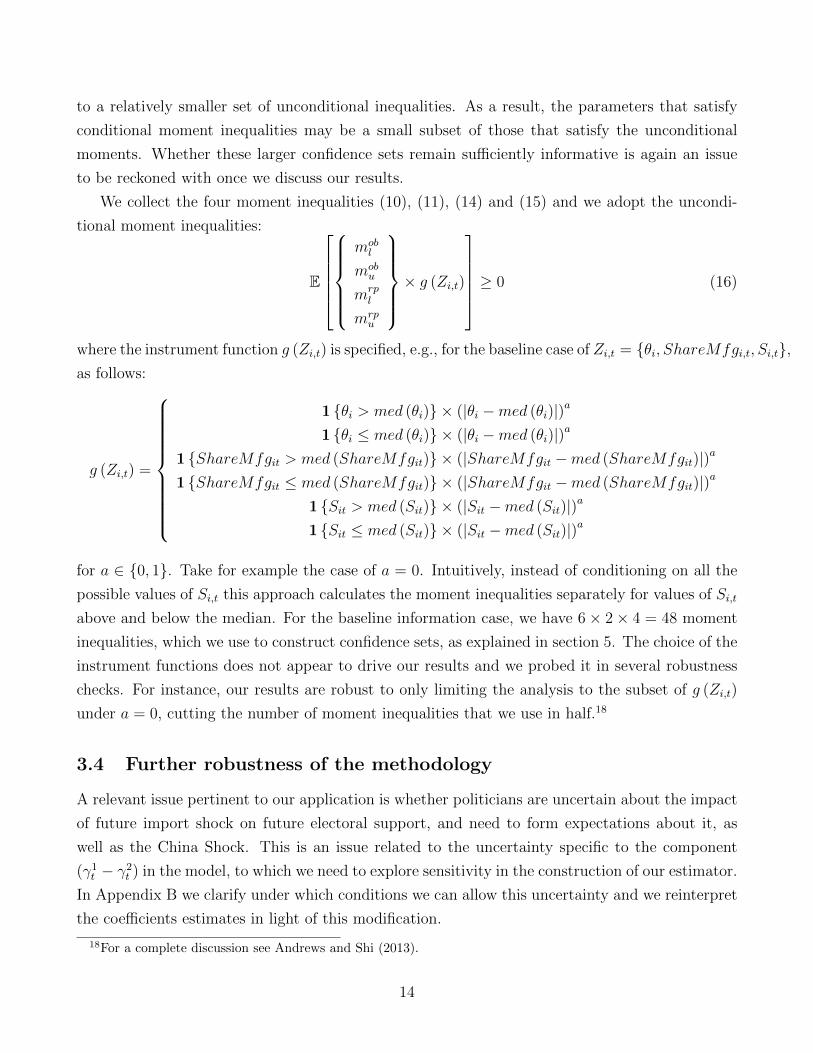
We collect the four moment inequalities (10), (11), (14) and (15) and we adopt the uncondi-

tional moment inequalities:

E

mobl

mobu

mrpl

mrpu

× g (Zi,t)

≥ 0 (16)

where the instrument function g (Zi,t) is specified, e.g., for the baseline case of Zi,t = θi, ShareMfgi,t, Si,t,as follows:

g (Zi,t) =

1 θi > med (θi) × (|θi −med (θi)|)a

1 θi ≤ med (θi) × (|θi −med (θi)|)a

1 ShareMfgit > med (ShareMfgit) × (|ShareMfgit −med (ShareMfgit)|)a

1 ShareMfgit ≤ med (ShareMfgit) × (|ShareMfgit −med (ShareMfgit)|)a

1 Sit > med (Sit) × (|Sit −med (Sit)|)a

1 Sit ≤ med (Sit) × (|Sit −med (Sit)|)a

for a ∈ 0, 1. Take for example the case of a = 0. Intuitively, instead of conditioning on all the

possible values of Si,t this approach calculates the moment inequalities separately for values of Si,t

above and below the median. For the baseline information case, we have 6× 2× 4 = 48 moment

inequalities, which we use to construct confidence sets, as explained in section 5. The choice of the

instrument functions does not appear to drive our results and we probed it in several robustness

checks. For instance, our results are robust to only limiting the analysis to the subset of g (Zi,t)

under a = 0, cutting the number of moment inequalities that we use in half.18

3.4 Further robustness of the methodology

A relevant issue pertinent to our application is whether politicians are uncertain about the impact

of future import shock on future electoral support, and need to form expectations about it, as

well as the China Shock. This is an issue related to the uncertainty specific to the component

(γ1t − γ2

t ) in the model, to which we need to explore sensitivity in the construction of our estimator.

In Appendix B we clarify under which conditions we can allow this uncertainty and we reinterpret

the coefficients estimates in light of this modification.

18For a complete discussion see Andrews and Shi (2013).

14

4 Institutional background and data

The background for the series of roll call votes that we employ in this paper is the extension of

Normal Trade Relations to the People’s Republic of China, after their suspension in 1951. NTR

status was restored in 1980 under Title IV of the Trade Act of 1974 and was dependent on the

presence of a bilateral trade agreement to be renewed every three years and on compliance with

the Jackson-Vanik amendment on freedom of emigration, required for Non-Market Economies.19

China’s NTR status would be renewed automatically every year upon the President recommen-

dation unless Congress disapproved it by enacting a joint resolution. It is widely recognized that

these resolutions were spurred by humanitarian and foreign policy considerations following the

Tiananmen Square events of 1989 (Pregelj, 1998). Congress sought to provide incentives, through

withholding of NTR status, to the Chinese government to address issues of human rights. In this

effort, it clashed with the executive branch, a fact reflected in the several episodes in which the

resolutions to disapprove NTR passed in the House, but died in the Senate or were overturned by

a Presidential veto. In light of these considerations, it should be clear that we do not view the

threat to local economic interests as the only driver of the legislators’ roll call votes, and ideological

considerations in the utility function of legislators account for this.

4.1 Roll call votes

The sample for our estimation includes individual legislator roll call votes for 12 House Joint

Resolutions that took place every year from 1990 to 2001, as listed in Table 1. Three of these

Joint Resolutions to disapprove NTR extension were passed by the House in the years 1990, 1991

and 1992, but not voted on or struck down in the Senate.20

The website voteview.com provides the roll call votes, together with the ICPSR code for each

legislator, the congressional district, the Party, and the first two dimensions of the DW-Nominate

score, a multidimensional scaling application developed by Poole and Rosenthal (1997) and the

first dimension of which is our proxy for θi.21 Instead of “Yea” and “Nay”, we indicate all votes

as Pro and Against China (NTR) for ease of interpretation (a “Yea” vote in favor of disapproving

China’s NTR is a vote against China).

Figure 1 shows that support for NTR is not purely along party lines and changes over time.

Democrats are relatively more supportive of NTR in the middle of the sample period, while

19See CRS Report for Congress Pregelj (2001) for further details.20Two House Resolutions, HR2212 and HR5318, in the 102nd Congress during the same period passed both in

the House and the Senate and were vetoed by President G.H.W. Bush.21voteview.com represents one of the most comprehensive and popular sources of measures of ideological positions

in American politics and is a standard reference in the political economy literature on Congress. See the Introductionfor references.

15

Republicans become increasingly supportive of NTR over time. There is substantial switching

of positions within individual legislators as well. Figures 2 and 3 show, by party, how many

legislators switch position or maintain their vote relative to the previous year. On average, every

year 15 percent (17 percent) of Republican (Democratic) legislators change their position relative

to the previous year. In sum, there is sufficient heterogeneity in positions across parties and within

legislators over time to justify that the changes in the electoral effects of the vote could play a role

beyond constant preferences and ideology of legislators.

We also include in the data the voting outcomes of the bill HR 4444 in 2000 which would grant

China permanent normal trade relations (PNTR) conditional on China’s accession to the WTO.

The results are stable regardless of the inclusion or exclusion of this bill.

Note that the period 1990-1992 covers the final years of the George H.W. Bush administration.

The period 1993-1996 coincides with the first Bill Clinton administration and the the period 1997-

2001 covers the second Clinton administration and the first year of the George W. Bush presidency.

Given the important role played by the executive branch in the legislative evolution of China’s

NTR status, this subdivision of the sample period is explored in our analysis, by allowing for

different parameters and expectations during each administration.

4.2 The China Shock

The exposure to the China Shock at the district level is generated from the import shocks in

different local labor markets nested within the district. We start with constructing the import

shocks at the level of commuting zones (CZs), which are clusters of adjoining counties characterized

by strong commuting ties and have been conceptualized as local labor markets in the literature

(Autor et al., 2013; Acemoglu et al., 2016). The shocks from different CZs are then aggregated to

congressional districts (CDs) similarly to Autor et al. (2020a).

4.2.1 Exposure to import shock at the commuting zone level

Future supply shocks from China faced by the commuting zone j is constructed according to:

Sj,t+1 =∑k

Ljk,tLj,t

∆M othk,t+1

Yk,t +Mk,t −Xk,t

. (17)

In this expression, ∆M othk,t+1 is the change in import of good k from China by eight other (non-U.S.)

high-income countries over 5 years in the future.22 It reflects the rising supply capacity of China

due to its economic reforms, and is arguably exogenous to the U.S. product-demand shocks from

22The eight other high-income countries are Australia, Denmark, Finland, Germany, Japan, New Zealand, Spain,and Switzerland.

16

the perspectives of the U.S. local economies (Autor et al., 2013; Acemoglu et al., 2016; Autor

et al., 2020b). The future import growth is then normalized by the contemporaneous absorption

(U.S. industry output plus net imports, Yk,t +Mk,t−Xk,t) at the industry level. Ljk,t/Lj,t denotes

the share of industry k in CZ j’s total employment in period t.

The Bartik-style measure (17) summarizes the exposure of CZ j to China’s future supply shocks

from the standpoint of t. Having a perfect foresight of (17) not only requires the information on

contemporaneous employment composition of the local labor market and domestic absorption of

different industries, but also knowledge on supply shocks from China 5 years in the future. In our

analysis, the future shocks correspond to the import supply growth over the period 1990-1995,

1991-1996, ..., 2001-2006, which overlaps with China’s post-WTO-accession period when the U.S.

witnessed the most intense increase in import competition from China.

While the congressional representatives may not have full knowledge of future import shocks

as in (17), they may use the information of the past shocks to form expectations. For the years

1993-2001, we construct import shock in the past 5 years analogously as follows:

Sj,t =∑k

Lik,t−5

Li,t−5

∆M othk,t

Yk,t−5 +Mk,t−5 −Xk,t−5

, (18)

where ∆M othk,t denotes the change in import of good k from China by eight other (non-U.S.)

high-income countries over the previous 5 years.23

The baseline measures (17) and (18) follow the specification in Acemoglu et al. (2016) and

Autor et al. (2020b), and can be derived from workhorse trade models with a gravity structure.

However, differently from the literature focusing on the impacts of contemporaneous trade shocks

on local economies, our study aims at evaluating the extent to which politicians foresaw the future

import shock from China in (17), and whether they acted on the relevant information when setting

China-specific trade policies.

23Due to data constraints, for years 1990-1992, we use the 2-year-lagged variables to construct the past shocks.To be specific, for t = 1990, 1991, 1992

Si,t =∑k

Lik,t−2

Li,t−2

∆Mothk,t

Yk,t−2 +Mk,t−2 −Xk,t−2,

where ∆Mothkt denotes the change in import of good k from China by eight other (non-US) high-income countries

over the past 2 years. As is discussed below, we use the data from County Business Patterns (CBP) to constructemployment shares. For 1990-1992, calculating Lik,t−5/Li,t−5 requires the 1985-1987 CBP data with industriesclassified based on 1977 SIC codes. For the purpose of analysis, the data needs to be mapped to the 1987 SICcodes. However, the crosswalk from 1977 SIC to 1987 SIC involves many splits of industries. As a result, theconcordance leads to a structural break in the employment measures for some localities over 1987-1988. For theconcern of systematic measurement errors, we don’t use the CBP data prior to 1988 for the main analysis.

17

4.2.2 Trade, employment and output data

This subsection describes the data sources that we employ to construct the commuting-zone-level

measures (17) and (18). Data on bilateral trade flows over the period 1988-2006 for the 4-digit

Standard International Trade Classification (SITC) industries are obtained from UN Comtrade

Database. We concord these data to four-digit Standard Industry Classification (SIC) industries.24

Following Autor et al. (2013) and Acemoglu et al. (2016), we aggregate together a few four-digit

industries to ensure compatibility with the additional data on employment discussed below. Our

final data set contains 397 manufacturing industries. We complement the trade data by the output

data obtained from the NBER-CES data. All import, export and output amounts are inflated to

2007 US dollars using the Personal Consumption Expenditure (PCE) deflator.

Information on industry employment structure by CZs over 1988-2001 is derived from the

County Business Patterns (CBP) data published by the US Census Bureau. The CBP tracks

employment, firm size distribution, and payroll by county and industry annually. To protect

confidentiality, employment for county-industry cells is sometimes reported as an interval instead

of exact count. We use the fixed-point imputation algorithm developed by Autor et al. (2013)

to derive employment for each county-industry cell. The county-level data is then aggregated to

commuting zones using the concordances provided by Autor et al. (2013).25

4.2.3 Exposure to import shocks at the congressional district level

Following Autor et al. (2020b), we map economic outcomes in CZs to CDs as follows. We start with

the geographic relationships between counties and congressional districts provided by the Missouri

Census Data Center (MCDC).26 Counties are sometimes split across different CDs, and the MCDC

concordance provides information on the distribution of the county population in each CD. We then

ascribe to each county-by-congressional district cell the CZ-level import shock that corresponds

to the county, and weight each cell by its share of population in the district. Lastly, we aggregate

the weighted shocks across cells to the CD level. By construction, if a district spans multiple CZs,

its exposure to China’s rising import competition is the population-share-weighted average of the

24The crosswalk that cross-matches the four-digit SITC (Rev.2) industries and the four-digit SIC (1987 version) isconstructed as follows. (1) We first map the four-digit SITC industries to the corresponding six-digit HarmonizedCommodity Description and Coding System (HS) products based on the concordance provided by UN WITS(https://wits.worldbank.org/product concordance.html). (2) We then apply the crosswalk from Autor et al. (2013),which assigns 6-digit HS products to 4-digit SIC industries. (3) Lastly, the four-digit SITC codes are cross-matchedwith the four-digit SIC codes based on their relations with the six-digit HS codes.

25Industry classifications in CBP changed periodically — over 1988-1997, employment is classified using theSIC (1987 version) codes, while employment thereafter is expressed according to the North American IndustryClassification System (NAICS). Using the crosswalk in Autor et al. (2013), we concord the post-1997 data to thefour-digit SIC industries.

26http://mcdc.missouri.edu/applications/geocorr1990.html

18

import shocks in these CZs. Since congressional districts, by construction, have similar population

size, they have roughly the same weight in our analysis. In the empirical analysis, we denote the

future and past import shocks at the CD level by Si,t+1 and Si,t, respectively.

During the sample period 1990-2001, the boundaries of county-by-congressional district cells

experienced a major change in 1993 but remained stable afterwards. Therefore, for 1990-1992, we

map the CZ-level import shocks to congressional districts as defined for the 102nd Congress. For

1993-2001, the mapping is based on the configuration of the 103rd Congress. This treatment does

not affect the consistency of our baseline analysis, because as is discussed below, we conduct the

estimation by periods based on presidential administrations, and none of the subsamples spans

over 1992-1993.

Figure 4 shows the cross-district averages of past and future import shocks. The import shocks

are always positive throughout the sample period, but the future shocks move less in tandem with

the past shocks in the later years. For the moment inequality estimation discussed in the following

section, we detrend the import shocks. The corresponding distributions reported in Table 2 reveal

a substantial heterogeneity in exposures across districts. For the periods 1997-2001, 1993-1996,

and 1990-1992, the interquartile ranges of future shock are 0.154, 0.078, and 0.143, respectively.

5 Results from congressional voting on trade relations with

China

5.1 Estimation results

This section reports our main results. To benchmark our approach to more standard methods

using incorrect proxies for the information set of politicians, we start by reviewing estimates of a

voting model using a maximum likelihood approach.

Table 3 shows that results substantially vary depending on the informational assumptions

made. An important parameter of interest is the weight placed by politicians on their affected

subconstituencies δt. A reasonable prior for this parameter would be a negative utility weight, δt <

0, placed on electoral groups adversely affected by the China Shock in the politician’s congressional

district (ceteris paribus, the politician wishes to minimize these adverse effects). While occasionally

the parameter estimates for δ are negative and sometimes of magnitude similar to those obtained

using the moment inequality approach, often the coefficients are economically insignificant and

not statistically different from zero. For example, for the period 1997-2001 the estimate for

δ is 0.018, which is small in absolute value relative to consistent estimates obtained with the

moment inequality method. The risk of attenuation from misspecification of the information set

of politicians is therefore evident in the MLE case. To further consolidate the intuition we also

19

offer Monte Carlo evidence of the problem in Appendix C.

We now proceed to the results of estimating of equation (5) using the three information sets

Zi,t: Minimal; Baseline; and Perfect Foresight. The 95% confidence sets that we report are built

through a grid search implementing the Generalized Moment Selection (GMS) method in Andrews

and Soares (2010) as detailed in Dickstein and Morales (2018). For each value of ωt we build a

modified method of moments (MMM) statistic, which tends to be large when, on average, the

moment inequalities are not satisfied at that value of the parameters. This is formally tested

by constructing the asymptotic distribution of the MMM statistic and rejecting ωt when the

MMM statistic is above the critical value corresponding to the 95th percentile of that distribution.

Incidentally, empty confidence sets instead have to be interpreted as highly significant rejection

(p-value < 0.05) of the corresponding information set. The steps to construct the 95% confidence

sets are detailed in Appendix D.

Table 5 reports estimation results splitting the NTR votes by presidential administration and

for the full sample 1990-2001. The first period 1990-1992 covers the George H.W. Bush adminis-

tration, the second period 1993-1996 coincides with the first Clinton administration, and the third

period 1997-2001 covers the second Clinton administration.27 Focusing on sub-periods allows for

heterogeneity in information and flexibility of the parameters with respect to the behavior of exec-

utive branch/agenda setting – a more robust approach that we prefer. Table 5 presents estimates

for the parameters at, bt and δt. We will mostly discuss results for the importance of constituency

interests δ, but we will gauge its magnitude in relation to the role of ideology parameter a.

Consider the pooled 1990-2001 results first. Panel A reports estimation results under the

assumption that the politicians’ information set includes at least the manufacturing share in their

district and their own ideology. Under this assumption we report a confidence set [−1.188,−0.137],

so that all values in the confidence set are negative, as we would expect if politicians are more

likely to vote against China’s NTR status when they expect their constituency to be exposed to

a larger shock. The confidence set is quite similar under the assumption of baseline information,

which includes also the current shock Si,t, [−1.275,−0.825].

The magnitude of the parameter δ can be illustrated as follows. Considering two districts

whose value of the China Shock are at the 25th and 75th percentile. The probability of voting in

favor of China’s NTR status decreases by between 0.035 and 0.053 when the value of the expected

China shock goes from its 25th percentile to its 75th percentile.28 This is a moderate effect,

27As a robustness check, we drop the year 2001, which overlaps with George W. Bush’s first year in office duringwhich the final vote took place, but was related to the previous administration’s efforts (Pregelj, 2001). The resultsremain similar.

28In particular, we calculate these percentage points as the minimum and maximum of

Φ(b+ δE

[Si,t+1|IBi,t

]75th)− Φ

(b+ δE

[Si,t+1|IBi,t

]25th)

evaluated at the mean θi = 0 and ωt ∈ Ω95%t ,

where Ω95%t is the 95 percent confidence set of the underlying parameters.

20

especially considering the role of ideology. If we perform the analogous exercise, we find that an

interquartile range shift in ideology (from relatively liberal to relative conservative) calculated at

the mean expected China shock value produces an increase in the probability of voting in favor of

China of between 0.134 and 0.174 in 1990-2001. In sum, these comparisons allow us to conclude

that the effect of ideology is much larger than the effect of constituent interests. These results line

up with common findings in the congressional voting literature for most bills (as early as Kalt and

Zupan (1984) and for a recent discussion see Poole and Rosenthal (2017)).

We will discuss differences in the parameters estimates between subsets of legislators after

introducing specification tests that allow us to gauge the information possessed by politicians.

5.2 Testing for different information sets

A fundamental first step in the analysis of politicians’ decisions is to assess the exact extent of

their information sets at the moment of the vote. A valid statistical approach to this form of

specification test is presented in Bugni et al. (2015). The test proposed by Bugni et al. (2015)

allows us to reject the null hypothesis that there exists a value of ωt within the parameter space

that can rationalize the set of moment inequalities presented in section 3.3. Specifically, consider

two alternative information sets Z1i,t and Z2

i,t. Intuitively, suppose there is no value of the parameter

vector for which the set of moment inequalities hold given Z1i,t, yet there are values of ωt within

the parameter space that can rationalize the set of moment inequalities given Z2i,t. Then one infers

that Z1i,t * Ii,t and cannot reject Z2

i,t ⊆ Ii,t. The rejection of the null in this framework may

also indicate misspecification of the original model of decision, so simple rejection of Z1i,t cannot

exclude misspecification per se. What is crucial in this application is that the failure to reject Z2i,t

eliminates this second interpretation of the test. Misspecification of the original model would affect

the analysis under both Z1i,t and Z2

i,t, as the decision model is unchanged and only the information

set varies across tests, and model misspecification would imply rejection in both instances.

Appendix D reports the full details for the construction of the BP, RC and RS specification

test statistics following Bugni et al. (2015) and the corresponding p-values. Generally speaking,

the test BP is less powerful than RC and RS, and rejection of the null hypothesis in any of these

tests indicates a rejection of the hypothesis that specific information belongs to the information

set of the members of Congress.

We report results for all three tests in Table 5. Columns 4, 5, and 6 report the p-values for BP,

RC and RS respectively. For the full sample and for two of the three presidential administration

periods we reject that politicians have perfect foresight, with p-values of 0.01-0.015 depending on

the test. For all periods we cannot reject that the politicians had at least the baseline information

set. While it is not obvious whether the baseline information set represents an optimal amount

21

of knowledge, we believe Table 4 is informative. It shows that the manufacturing employment

share and past import shock have significant explanatory power in predicting future shocks. The

R-squared is generally around 55 percent and is lower in the later period, suggesting that the

variance of the expectational errors have increased over time and close to the end of the sample.

Our results point to information used by politicians worsening over time and their capacity of

forecasting the China Shock in the following five years deteriorating. Why would legislators be

better informed in the earlier part of the period? We hypothesize that this is due to the more

predictable nature of the shocks in the early 1990s, when China was specialized in relatively less

complex and more labor intensive products. In Figure 5 we report the autocorrelation of the

China Shock at the industry level and it is clear that in the earlier years the shock was more

predictable from year to year as the autocorrelation was above 0.3. In the second half of the 1990s

the autocorrelation progressively drops to zero, a fact that could justify why politicians were less

than perfectly informed as the 2000s approached. This is compatible with the evolution of China’s

comparative advantage from low value-added to more complex products over time.

Our evidence on the extent of the information set of U.S. politicians and our assessment of

their (fairly accurate) predictions on the sectoral consequences of the China Shock is in line with

evidence concerning expectations of other types of actors. Greenland et al. (2020) find that equity

valuations around the key PNTR vote in Congress correlated with US firms’ exposure to trade

liberalization with China, supporting the view that stock market participants were systematically

pricing firms and sectors exposure to the shock.29 It is therefore not completely implausible that

U.S. legislators had information sets comparable with those of financial agents.

5.3 Heterogeneity across groups of politicians

5.3.1 Party

The estimates and tests presented so far were performed in the universe of the members of Congress

during the 1990-2001 period under an assumption of common information sets. It is plausible to

hypothesize that politicians from different parties, and with different electoral prospects, might

have had varying degrees of knowledge and different expectations.

In this section we analyze three dimensions of heterogeneity: political party, tenure in office

(i.e., experience), and margin of victory in the most recent election. For all tests we report the

results for the baseline information set. To anticipate our findings, the picture that will emerge

from this heterogeneity analysis is that Democrats at the time of NTR votes were both more

informed and more sensitive to constituent interests than Republicans, and that legislators in

29For a discussion on the degree of predictability of trade policy change effects based on stock reactions of bothdomestic and foreign firms see also Breinlich (2014).

22

tighter electoral races placed a heavier weight on the China Shock.

In Table 6 we find that Democrats are more informed than Republicans, as we cannot reject

that Democrats had at least the baseline information set in all time periods, but we can reject

at standard levels of significance that Republicans know the baseline information in all periods,

but 1990-1992. When we obtain non-empty parameter estimates, we find that Democrats display

higher (in absolute value) sensitivity to the China Shock. Republicans’ confidence set for δ strad-

dles zero, while the entire confidence set for the Democratic members of the House is comprised

of negative values. This is in line with Democratic legislators historical alignment with workers’

interests and placing more weight on the affected subconstituencies (Poole and Rosenthal, 1997).30

To further establish the relevance of this dimension of heterogeneity, we also considered be-

havior of politicians beyond voting, particularly congressional speech (number of speeches related

to the “China and trade” issue or the “China and labor” issue delivered). We can see that the

non-voting data aligns with preference and information patterns that we reported. We only focus

on two corroborating findings here and present a full analysis in Appendix A.2. First, as the China

Shock over 2001-2006 is realized, representatives from districts in the top tercile of the exposure

to import shock from China raise the related trade and labor issues more often in their speeches,

but such response is stronger for Democrats than Republicans. Second, consistently with their

higher information and preference weights, Democrats start taking actions earlier. Specifically, for

Democrats the congressional speech on China starts surging during the 106th Congress, 1999-2000,

while for Republicans, the effect picks up in the 108th, 2001-2002.

5.3.2 Vote margins and tenure

In Table 7 we also explore whether politicians with above-median victory margins in the previous

election display differences in the sensitivity to constituent interests. The literature has found

higher sensitivity for legislators in tighter races (Mian et al., 2010). We indeed find that, across

different periods, legislators in tighter races display confidence sets for δ that are entirely composed

of negative values, whereas confidence sets for politicians in safe races often cover both positive

and negative values, consistent with lower preference weights. It does not appear to be the case,

however, that politicians in tight races were differentially informed relative to politicians elected

by larger margins. While it is not an objective of this section to identify whether the heightened

sensitivity to the China Shock was due to state dependent preferences of politicians, changing with

electoral conditions, or due to selection (although this should also reflect in different information

sets), the analysis does display a potential for our approach to pick up differential elements of the

behavior and knowledge of sub-groups of politicians.

30In Appendix E.2 we further discuss through Monte Carlo simulations the role of misspecifications of informationsets with respect to heterogeneity across levels of ideology θ.

23

Finally, we explore the role of experience. In Table 8 we divide the sample in two according to

whether House members tenure is above or below the median. One may imagine that politicians

that are very experienced have better access to various sources of information. We do not find

support for this conjecture, as confidence sets for δ of junior legislators appear not systematically

different from those of senior ones.

5.4 Validation: NTR votes for Vietnam

As validation of our model and methodology, we briefly compare the results for the analysis of

the NTR votes for China to a set of similar, but distinct NTR votes for the case of Vietnam. The

goal here is to establish comparability in the responses of politicians across sets of votes. We view

this as a way of supporting external validity of our findings.

The analysis covers the votes on Vietnam’s Jackson-Vanik Waiver (necessary to extend Viet-

nam’s NTR status) that took place over the period 1998 to 2002. Based on a report by the

Congressional Research Services, disapproval resolutions were not introduced in 2003, 2004, or

2005 (i.e. there is no voting data over 2003-05). In 2006, the House passed legislation to grant

Vietnam permanent normal trade relations (PNTR) status as part of a more comprehensive trade

bill and Vietnam accessed the WTO in 2007.31

In Table 9 the coefficient δ appears larger in magnitude than for the China Shock case. Specif-

ically, the baseline confidence set is [−74.075,−6.700]. However, this is because, as expected, the

magnitude of the import shock from Vietnam is several orders smaller than that from China. The

standard deviation of future import shock from Vietnam is 0.006, while that from China in the

same period is 0.129. Adjusted for this scaling, the economic significance of constituency interests

appears small for the Vietnam case as well, consistent with our findings of a low constituent weight

estimated with the China NTR votes.

Concerning information sets, Table 9 confirms that members of Congress were informed about

the impact of Vietnamese imports to some extent, as they were for China.32 We cannot reject at

standard significance levels the baseline information set, however, we reject that politicians have

perfect foresight. Overall, across the sets of NTR votes for Vietnam and China, we do not find

salient differences both in terms of economic magnitude of constituent weights and information

sets.

31See Appendix A for additional details on the data. Due to the congressional redistricting in 2002, for theanalysis in this section, we only include the bills over 1998-2001. The past and future import supply shocks fromVietnam are constructed analogously to the China Shock in section 4.2.

32The manufacturing employment share and past import shock also have significant explanatory power in pre-dicting future shocks for the case of Vietnam. The R-squared is generally around 53 percent.

24

5.5 Role of special interests

Special interests’ contributions33 are often listed within the set of potential drivers of congressional

voting, but not without substantial uncertainty about the economic magnitude of their effect.

There is evidence of a prominent role of special interest giving in certain votes (e.g. the EESA

of 2008, see Mian et al., 2010), but no consensus in the political economy literature on its role

for the bulk of all congressional activity (Stratmann, 2005). In the case of China’s NTR, we find

no clear evidence that special interests, both in terms of campaign contributions from business

organizations (corporations and business associations) or from labor unions, played a crucial role

in driving congressional votes, beyond ideology and constituent interests in our main specification.

We base this assessment on three main sets of empirical evidence which we report below.

First, as an extra dimension of heterogeneity, we separated politicians into two groups, depend-

ing on whether the campaign contributions from business interests are above or below the median

in the sample. The degree of heterogeneity found in Table 10 is minimal, with marginally more

negative estimates of constituent weights for politicians with contributions above the median in

later periods. This may suggest that money in politics may target politicians with some type of

characteristics, but ultimately the confidence sets do not point to substantial differences.

Second, we augmented our specification with campaign contributions. It has to be noted that

adding elements to the vector of parameters within the moment inequality approach is extremely

costly, due to the grid search process necessary for inference and hypothesis testing. Further,

contributions could be endogenous to NTR votes, and hence it may be difficult to interpret the

additional parameters. Table A.1 in Appendix F report the results. Due to the computational

burden, we consider the following specifications, each with four parameters to estimate and infor-

mation sets to assess: (a) Baseline specification + campaign contributions from business organi-

zations (Panel A); (b) Baseline specification + campaign contributions from labor unions (Panel

B); (c) Baseline specification + the second principal component of contributions from business

organizations and labor unions34 (Panel C). Our main results appear robust to this inclusion and

its additional explanatory power is limited.

Third, we explore the congressional committees closer to the policy decision and likely the

33The data on campaign donations employed in the analysis of special interests are obtained from opensecrets.org,based on official Political Action Committee disclosure forms from the U.S. Federal Election Commission. opense-crets.org is a website run by the Center for Responsive Politics, one of the main nonpartisan organizations inWashington DC, dedicated to electoral transparency and to the collection of information related to campaignspending and lobbying disclosures.

34Note that for the first principal component, the loadings on contributions from business and labor are bothpositive. Hence, the first component may just capture the fact that both interest groups are trying to curry favorfrom more influential representatives. For the second principal component, the loading on money from businessis positive and the loading on money from labor is negative. So, it may be a summary statistics for the specialinterests in favor of a normal trade relationship with China.

25

most important targets for special interests. In particular, we exclude the politicians working in

influential committees (including the Commerce, and Ways and Means committees), who may be

more influenced by money in politics. As is reported in Table A.2 in Appendix F, our results

remain robust to this approach.

5.6 Further robustness

In Appendix E, we enrich the results by presenting a number of extensions and robustness analysis.

Appendix E.1 discusses through Monte Carlo simulations the potential biases in our analysis due to

violations of the rational expectation assumption. In particular, it introduces a constant under- or

over-prediction of the China Shock, expectational errors correlated with Si,t and errors correlated

with θi. In this particular setting, estimation based on moment inequalities and specification

tests appear to be robust to moderate violations of rational expectations. Exceptions typically

emerge in cases where the variation in irrational expectational errors is larger than the variation in

unpredictable components of the China Shock (i.e., the component of Si,t+1 that is unexplained by

elements in I). Appendix E.3 introduces the “NTR gap” as defined by Pierce and Schott (2016)

in the formulation of the China Shock. This takes into account that votes to remove NTR status

would be more effective at reducing imports from China for goods where the difference between

the MFN tariff and the “Column 2” tariff was larger. Appendix E.4 introduces export shocks and

finds a positive effect of export opportunities on the probability of a vote in favor of China’s NTR

status. Yet, the information tests and the other parameters remain largely consistent with the

main findings.

6 Counterfactuals

In this section we employ the estimated parameters of the model to perform two counterfactuals

that answer the following questions: (i) Would giving full information to legislators have changed

the results of the NTR roll call votes? (ii) Would the results of the NTR votes have changed if

legislators placed a larger weight on the labor market consequences of the China Shock?

6.1 Legislators receiving information about the China Shock

After establishing that, for most of the time period in our sample, politicians had less than perfect

knowledge of the labor market consequences of China’s export expansion, a natural question we

can ask is whether providing more accurate information to politicians would have changed their

vote, and the overall passage of certain bills. The answer, for the case of China NTR votes, is not

substantially.

26

As the construction of the counterfactual is not trivial and not commonplace in the literature,

we provide some details. Conditional on a particular value of the parameter vector ωt = at, bt, δt,and information set Ii,t, the decision of voting in favor of China is given by:

Yi,t(ωt, Ii,t, ξi,t) = atθi + bt + δtE[Si,t+1|Ii,t]− ξi,t ≥ 0 .

Integrating Yi,t(ωt, Ii,t, ξi,t) over ξi,t generates the probability that politician i casts a pro-China

vote in period t. In particular,∫ξi,t

Yi,t(ωt, Ii,t, ξi,t)φ(ξi,t)dξi,t =

∫ξi,t

1 atθi + bt + δtE[Si,t+1|Ii,t]− ξi,t ≥ 0φ(ξi,t)dξi,t.

Denote by Nt the set of politicians in period t, the share of votes in favor of China is then given

by:

Π+(ωt, Ii,t,Nt) =1

Nt

∑i∈Nt

∫ξi,t

Yi,t(ωt, Ii,t, ξi,t)φ(ξi,t)dξi,t.

The corresponding 95 percent confidence set of the number of politicians vote in favor of China is:[min

ωt∈Ω95%t

Π+(ωt, Ii,t,Nt)

, maxωt∈Ω95%

t

Π+(ωt, Ii,t,Nt)

],

where Ω95%t is the 95 percent confidence set for the underlying parameters.

We simulate Π+(ωt, Ii,t,Nt) under the case of baseline information Ibi,t and the case of perfect

foresight Ipi,t. The change in share of votes (in percentage point) in favor of China when we provide

politicians with full information is:[min

ωt∈Ω95%t

Π+(ωt, Ipi,t,Nt)− Π+(ωt, Ibi,t,Nt)

× 100, max

ωt∈Ω95%t

Π+(ωt, Ipi,t,Nt)− Π+(ωt, Ibi,t,Nt)

× 100

].

Before we delve into the specific results, it is worth pointing out that the effect of information

provision on NTR votes is ambiguous, and depends on (i) the underlying distribution of the

expectational errors G(εi,t+1), (ii) the weight on constituent interests that is governed by δt, and

(iii) the policy position relative to individual ideology atθi + bt. To see this, given the assumption

of normal distribution and with a large sample, the change of vote share in favor of NTR with

China can be written as:

27

Π+(ωt, Ipi,t,Nt)− Π+(ωt, Ibi,t,Nt)

=1

Nt

∑i∈Nt

[Φ(atθi + bt + δtSi,t+1)− Φ(atθi + bt + δtE[Si,t+1|Ibi,t])]

=

∫εi,t+1

[Φ(atθi + bt + δtE[Si,t+1|Ibi,t] + δtεi,t+1)− Φ(atθi + bt + δtE[Si,t+1|Ibi,t])]dG(εi,t+1)(19)

Regarding (i), our assumption of rational expectations dictates that εi,t+1 has a mean zero, condi-

tional on Ibi,t. Moreover, as is shown in Figure 6, the expectation errors are more or less symmet-

rically distributed in different sample periods. In Figure 7, we illustrate the roles of (ii) and (iii)

given a symmetric distribution of εi,t+1. Point A represents the probability of casting a pro-China

vote for legislators who are endowed with θi and have an expectation E[Si,t+1|Ibi,t]. Note that

in this scenario, the general policy position is in favor of China, and point A is located in the

concave segment of Φ(·). (This scenario is likely the case during 1993-1996 when the vote share

in favor of China was above 70 percent on average.) When these politicians are supplied with

complete information, they are facing import shocks Si,t+1 that are dispersed around E[Si,t+1|Ibi,t]in a mean-preserving way. As is represented by point B, the share of pro-China vote will be lower

in the counterfactual due to the concavity of Φ(·) at this segment. The magnitude of the counter-

factual change hinges on the dispersion of δtεi,t+1, which in turn depends on δt and the variation

of εi,t+1. In section 5, we show that the effect of constituent interests reflected by the estimate of

δ is moderate, and that the covariates in the baseline information set have significant explanatory

power in predicting future shock especially in the earlier period (i.e., the variation of expectational

errors is also moderate). These findings indicate that the effect of improving information could

be small. Points C and D in Figure 7 depict the case in which general policy position is against

China, and point C is located in the convex segment of Φ(·). (This is related to the scenario in

1990-1992 when the vote share in favor of China was around 40 percent on average.) Under this

case, had the politicians been provided with complete information on Si,t+1, the pro-China vote

share would have increased. The magnitude of the counterfactual change again depends on δt and

the variance of εi.t+1.

We also simulate the number of politicians who vote for China in the baseline, but switch vote

28

in the counterfactual according to

N+−(ωt, Ibi,t → Ipi,t,Nt)

=

∫ξ,t

Yi,t(ωt, Ibi,t, ξi,t)(1− Yi,t(ωt, Ipi,t, ξi,t))φ(ξi,t)dξi,t

=

∫ξi,t

1atθi + bt + δtE[Si,t+1|Ibi,t]− ξi,t ≥ 0

1atθi + bt + δtE[Si,t+1|Ipi,t]− ξi,t < 0

φ(ξi,t)dξi,t.

Analogously, we can derive the number of politicians in the other categories: vote in favor of China

in both the baseline and the counterfactual, vote against China in the baseline and switch in the

counterfactual, and vote against China in both scenarios. The share of politicians for each of the

cases, and the corresponding confidence sets are defined accordingly.

Table 11 shows the results of this counterfactual exercise. There are only a few small changes

in the voting patterns across politicians who now possess full information, a result of the fact

that they already possess a substantial amount of information to begin with and that the weight

on constituent interests is moderate. Moreover, the vote share in favor of China’s NTR status

appears unaffected.35

6.2 Counterfactual: Heightened constituent interests

Another counterfactual that we explore here involves increasing the legislator’s weight placed on

his or her local constituents. Specifically, we apply the lower bounds of δt corresponding to the

confidence sets of two groups of politicians (i) Democrats and (ii) politicians with below median

victory margins in the previous election to all politicians, and then simulate the NTR votes. As is

demonstrated in section 5.3, both these groups place high weight on the subconstituencies affected

by the China Shock. By setting δt at the highest possible (absolute) values, we assess whether

this margin of preferences may have played an important role in driving legislative outcomes for

given expectations of the legislators.

Table 12 reports the confidence sets of the simulated vote shares. For all the simulations,

we assume that politicians have access to the baseline information set and make voting decisions

based on E[Si,t+1|Ibi,t]. In Panel A, we simulate the shares of pro-China votes based on the baseline

estimates reported in Table 5. The predicted vote shares in favor of China align with the actual

shares.

In Panel B, we apply the largest possible weight that Democrats place on the expected China

shock to all politicians. The counterfactual weight in 1997-2001 (respectively, 1993-1996 and 1990-

1992) is nearly three times (respectively, two times and three times) larger than the lower bound

35Also note that in aggregate the counterfactual change in pro-China vote share in 1993-1996 is negative, whilethat in 1990-1992 is positive, which is consistent with the scenarios depicted in Figure 7.

29

of the baseline estimates of δt. The simulated vote share is in the range of [15.711, 30.443] in 1997-

2001, indicating that bills in favor of NTR with China would have not passed in this counterfactual

scenario during this period. The only caveat is that the confidence set of the counterfactual vote

share still straddles 50 percent for the period 1993-1996.

Panel C applies to all legislators the largest possible weight placed by the politicians facing

high electoral pressure (i.e., winning margins below median). In this counterfactual, the passage

of the bills in favor of NTR with China would have been overturned in 1993-1996, but not in

1997-2001.

7 Conclusion

China’s permanent NTR status in the U.S. and its accession to the WTO possibly represent one

of the most salient critical junctures in international trade (and certainly in trade policy decisions)

of the last fifty years. This paper investigates whether U.S. politicians had imperfect information

about the extent of China Shock’s repercussions in their home district at the time when they

repeatedly voted on China’s Normal Trade Relations status between 1990 and 2001.

To isolate the role of preferences versus information of members of Congress, we present a

voting model and an application of a method of moment inequality approach designed to estimate

expectations in decision making and to formally test for the content of information sets of legis-

lators. We find that U.S. legislators had imperfect, but fairly accurate expectations, yet placed a

relatively low weight on the constituencies that ended up being adversely affected by the China

Shock.

The approach discussed in this paper may be a general and informative avenue for the study of

policy decisions made by politicians and to understand their expectations. Being able to resolve

across preference and information margins is a valuable step forward for political economy and po-

litical science scholars interested in both questions of political accountability and learning in policy

making. Future research should implement and extend our application outside the consequential

questions of trade policy that we address in this paper, including labor, housing, healthcare, and

fiscal policy.

30

References

Acemoglu, D., Autor, D., Dorn, D., Hanson, G. H., Price, B., 2016. Import competition and the

great us employment sag of the 2000s. Journal of Labor Economics 34 (S1), S141–S198.

Ahn, H., Manski, C. F., 1993. Distribution theory for the analysis of binary choice under uncer-

tainty with nonparametric estimation of expectations. Journal of Econometrics 56 (3), 291–321.

Alesina, A., 1988. Macroeconomics and politics. NBER macroeconomics annual 3, 13–52.

Alesina, A., Miano, A., Stantcheva, S., 2020. The polarization of reality. In: AEA Papers and

Proceedings. Vol. 110. pp. 324–28.

Alesina, A., Tabellini, G., 1990. A positive theory of fiscal deficits and government debt. The

Review of Economic Studies 57 (3), 403–414.

Andrews, D. W., Shi, X., 2013. Inference based on conditional moment inequalities. Econometrica

81 (2), 609–666.

Andrews, D. W., Soares, G., 2010. Inference for parameters defined by moment inequalities using

generalized moment selection. Econometrica 78 (1), 119–157.

Autor, D., Dorn, D., Hanson, G., 2019. When work disappears: Manufacturing decline and the

falling marriage market value of young men. American Economic Review: Insights 1 (2), 161–78.

Autor, D., Dorn, D., Hanson, G., Majlesi, K., 2020a. Importing political polarization? the electoral

consequences of rising trade exposure. American Economic Review 110 (10), 3139–83.

Autor, D., Dorn, D., Hanson, G., Majlesi, K., 2020b. Importing political polarization? the electoral

consequences of rising trade exposure. American Economic Review 110 (10), 3139–83.

Autor, D. H., Dorn, D., Hanson, G. H., 2013. The china syndrome: Local labor market effects of

import competition in the united states. American Economic Review 103 (6), 2121–68.

Autor, D. H., Dorn, D., Hanson, G. H., 2016. The china shock: Learning from labor-market

adjustment to large changes in trade. Annual Review of Economics 8, 205–240.

Baldwin, R. E., Magee, C. S., 2000. Is trade policy for sale? congressional voting on recent trade

bills. Public Choice 105 (1-2), 79–101.

Bateman, D. A., Clinton, J., Lapinski, J. S., 2017. A house divided? political conflict and polar-

ization in the u.s. congress, 1877- 2011. American Journal of Political Science 61 (3), 698–714.

31

Blanchard, E. J., Bown, C. P., Chor, D., 2019. Did trump’s trade war impact the 2018 election?

Tech. rep., National Bureau of Economic Research.

Breinlich, H., 2014. Heterogeneous firm-level responses to trade liberalization: A test using stock

price reactions. Journal of International Economics 93 (2), 270–285.

Bugni, F. A., Canay, I. A., Shi, X., 2015. Specification tests for partially identified models defined

by moment inequalities. Journal of Econometrics 185 (1), 259–282.

Canen, N., Kendall, C., Trebbi, F., 2020. Unbundling polarization. Econometrica 88 (3), 1197–

1233.

Che, Y., Lu, Y., Pierce, J. R., Schott, P. K., Tao, Z., 2020. Does trade liberalization with china

influence us elections? Tech. rep., National Bureau of Economic Research.

Clinton, J., Jackman, S., Rivers, D., 2004. The statistical analysis of roll call data. American

Political Science Review 98 (2), 355–370.

Colantone, I., Stanig, P., 2018. The trade origins of economic nationalism: Import competition

and voting behavior in western europe. American Journal of Political Science 62 (4), 936–953.

Dickstein, M. J., Morales, E., 2018. What do exporters know? The Quarterly Journal of Economics

133 (4), 1753–1801.

Drazen, A., Masson, P. R., 1994. Credibility of policies versus credibility of policymakers. The

Quarterly Journal of Economics 109 (3), 735–754.

Fajgelbaum, P. D., Goldberg, P. K., Kennedy, P. J., Khandelwal, A. K., 2020. The return to

protectionism. The Quarterly Journal of Economics 135 (1), 1–55.

Feenstra, R. C., Ma, H., Xu, Y., 2019. Us exports and employment. Journal of International

Economics 120, 46–58.

Feigenbaum, J. J., Hall, A. B., 2015. How legislators respond to localized economic shocks: Evi-

dence from chinese import competition. The Journal of Politics 77 (4), 1012–1030.

Feler, L., Senses, M. Z., 2017. Trade shocks and the provision of local public goods. American

Economic Journal: Economic Policy 9 (4), 101–43.

Fenno, R. F., 1978. Home Style: House Members in their Districts. Boston: Little, Brown.

Gentzkow, M., Shapiro, J. M., Taddy, M., 2019. Measuring group differences in high-dimensional

choices: method and application to congressional speech. Econometrica 87 (4), 1307–1340.

32

Greenland, A., Ion, M., Lopresti, J., Schott, P., 2020. Using equity market reactions to infer

exposure to trade liberalization.

Greenland, A., Lopresti, J., 2016. Import exposure and human capital adjustment: Evidence from

the us. Journal of International economics 100, 50–60.

Greenland, A., Lopresti, J., McHenry, P., 2019. Import competition and internal migration. Review

of Economics and Statistics 101 (1), 44–59.

Heckman, J. J., Snyder, J. M., 1997. Linear probability models of the demand for attributes with

an empirical application to estimating the preferences of legislators. The RAND Journal of

Economics 28.

Ho, K., Pakes, A., 2014. Hospital choices, hospital prices, and financial incentives to physicians.

American Economic Review 104 (12), 3841–84.

Jenkins, J. A., 2000. Examining the robustness of ideological voting: evidence from the confederate

house of representatives. American Journal of Political Science, 811–822.

Jones, B. D., Baumgartner, F. R., 2005. The politics of attention: How government prioritizes

problems. University of Chicago Press.

Kalt, J. P., Zupan, M. A., 1984. Capture and ideology in the economic theory of politics. The

American Economic Review 74 (3), 279–300.

Kalt, J. P., Zupan, M. A., 1990. The apparent ideological behavior of legislators: Testing for

principal-agent slack in political institutions. The Journal of Law and Economics 33 (1), 103–

131.

Krehbiel, K., 1992. Information and legislative organization. University of Michigan Press.

Ladewig, J. W., 2010. Ideological polarization and the vanishing of marginals: Retrospective roll-

call voting in the us congress. The Journal of Politics 72 (2), 499–512.

Levitt, S. D., 1996. How do senators vote? disentangling the role of voter preferences, party

affiliation, and senator ideology. The American Economic Review 86 (3), 425–441.

Manski, C., 1991. Nonparametric estimation of expectations in the analysis of discrete choice under

uncertainty. In: nonparametric and Semiparametric methods in Econometrics and Statistics:

proceedings of the fifth International Symposium in Economic Theory and Econometrics. Vol. 5.

Cambridge University Press, p. 259.

33

McCarty, N., Poole, K. T., Rosenthal, H., 2006. Polarized America: The Dance of Ideology and

Unequal Riches. Cambridge: MIT Press.

Mian, A., Sufi, A., Trebbi, F., December 2010. The political economy of the us mortgage default

crisis. American Economic Review 100 (5).

Mian, A., Sufi, A., Trebbi, F., 04 2014. Resolving debt overhang: Political constraints in the

aftermath of financial crises. American Economic Journal: Macroeconomics 6 (2), 1–28.

Moskowitz, D. J., Rogowski, J., Jr., J. M. S., 2017. Parsing party polarization, mimeo.

Peltzman, S., 1984. Constituent interest and congressional voting. The Journal of Law and Eco-

nomics 27 (1), 181–210.

Pierce, J. R., Schott, P. K., 2016. The surprisingly swift decline of us manufacturing employment.

American Economic Review 106 (7), 1632–62.

Poole, K., Rosenthal, H., 2017. Ideology and Congress: A Political Economic History of Roll Call

Voting. 2nd Edition Routledge.

Poole, K. T., Rosenthal, H., 1984. The polarization of american politics. Journal of Politics 46 (4),

1061–1079.

Poole, K. T., Rosenthal, H., 1997. Congress: A Political-Economic History of Roll Call Voting.

New York: Oxford University Press.

Pregelj, V. N., 1998. Most-favored-nation status: Congressional consideration, 1989-1998. Tech.

rep., Congressional Research Service.

Pregelj, V. N., 2001. Most-favored-nation status of the people’s republic of china. Tech. rep.,

Congressional Research Service.

Primiceri, G. E., 2006. Why inflation rose and fell: policy-makers’ beliefs and us postwar stabi-

lization policy. The Quarterly Journal of Economics 121 (3), 867–901.

Rodrik, D., 1995. Political economy of trade policy. Handbook of international economics 3, 1457–

1494.

Sargent, T., Williams, N., Zha, T., 2006. Shocks and government beliefs: The rise and fall of

american inflation. American Economic Review 96 (4), 1193–1224.

Stimson, J. A., MacKuen, M. B., Erikson, R. S., 1995. Dynamic representation. American political

science review, 543–565.

34

Stratmann, T., 2005. Some talk: Money in politics. a (partial) review of the literature. In: Policy

challenges and political responses. Springer, pp. 135–156.

35

Figure 1: Roll call votes Pro China by Party

84 90 92

112

56

79

210

108

215

141 143

178

119

167

112

147

115

149

110

150

117

164

102

157

050

100

150

200

1990 1991 1992 1993 1994 1995 1996 1997 1998 1999 2000 2001

Votes pro China NTR RepublicanVotes pro China NTR Democrat

36

Figure 2: Roll call vote switching - Democrats

050

100

150

200

1991 1992 1993 1994 1995 1996 1997 1998 1999 2000 2001

Con → Pro Pro → ConStay Pro Stay Con

Figure 3: Roll call vote switching - Republicans

050

100

150

1991 1992 1993 1994 1995 1996 1997 1998 1999 2000 2001

Con → Pro Pro → ConStay Pro Stay Con

37

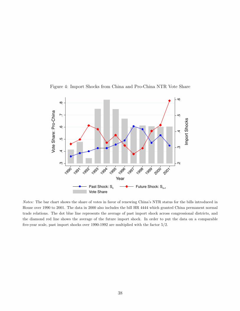
Figure 4: Import Shocks from China and Pro-China NTR Vote Share

.2.3

.4.5

.6

Impo

rt Sh

ocks

.3.4

.5.6

.7.8

Vote

Sha

re: P

ro-C

hina

1990

1991

1992

1993

1994

1995

1996

1997

1998

1999

2000

2001

Year

Past Shock: Sit Future Shock: Sit+1

Vote Share

Notes: The bar chart shows the share of votes in favor of renewing China’s NTR status for the bills introduced in

House over 1990 to 2001. The data in 2000 also includes the bill HR 4444 which granted China permanent normal

trade relations. The dot blue line represents the average of past import shock across congressional districts, and

the diamond red line shows the average of the future import shock. In order to put the data on a comparable

five-year scale, past import shocks over 1990-1992 are multiplied with the factor 5/2.

38

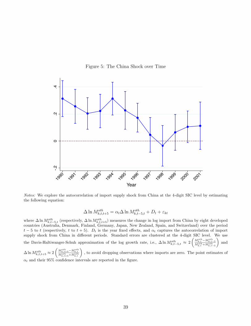
Figure 5: The China Shock over Time

-.20

.2.4

1990

1991

1992

1993

1994

1995

1996

1997

1998

1999

2000

2001

Year

Notes: We explore the autocorrelation of import supply shock from China at the 4-digit SIC level by estimatingthe following equation:

∆ lnM othk,t,t+5 = αt∆ lnM oth

k,t−5,t +Dt + εkt

where ∆ lnMothk,t−5,t (respectively, ∆ lnMoth

k,t,t+5) measures the change in log import from China by eight developedcountries (Australia, Denmark, Finland, Germany, Japan, New Zealand, Spain, and Switzerland) over the periodt − 5 to t (respectively, t to t + 5). Dt is the year fixed effects, and αt captures the autocorrelation of importsupply shock from China in different periods. Standard errors are clustered at the 4-digit SIC level. We use

the Davis-Haltiwanger-Schuh approximation of the log growth rate, i.e., ∆ lnMothk,t−5,t ≈ 2

(Moth

k,t −Mothk,t−5

Mothk,t +Moth

k,t−5

)and

∆ lnMothk,t,t+5 ≈ 2

(Moth

k,t+5−Mothk,t

Mothk,t+5+Moth

k,t

), to avoid dropping observations where imports are zero. The point estimates of

αt and their 95% confidence intervals are reported in the figure.

39

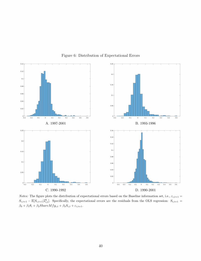
Figure 6: Distribution of Expectational Errors

-0.3 -0.2 -0.1 0 0.1 0.2 0.3 0.4 0.5 0.60

0.02

0.04

0.06

0.08

0.1

0.12

0.14

A. 1997-2001

-0.3 -0.2 -0.1 0 0.1 0.2 0.3 0.4 0.50

0.05

0.1

0.15

0.2

0.25

B. 1993-1996

-0.3 -0.2 -0.1 0 0.1 0.2 0.3 0.4 0.50

0.05

0.1

0.15

0.2

0.25

C. 1990-1992

-0.4 -0.3 -0.2 -0.1 0 0.1 0.2 0.3 0.4 0.5 0.60

0.02

0.04

0.06

0.08

0.1

0.12

0.14

0.16

D. 1990-2001

Notes: The figure plots the distribution of expectational errors based on the Baseline information set, i.e., εi,t+1 =

Si,t+1 − E[Si,t+1|Ibi,t]. Specifically, the expectational errors are the residuals from the OLS regression: Si,t+1 =

β0 + β1θi + β2ShareMfgi,t + β3Si,t + εi,t+1.

40

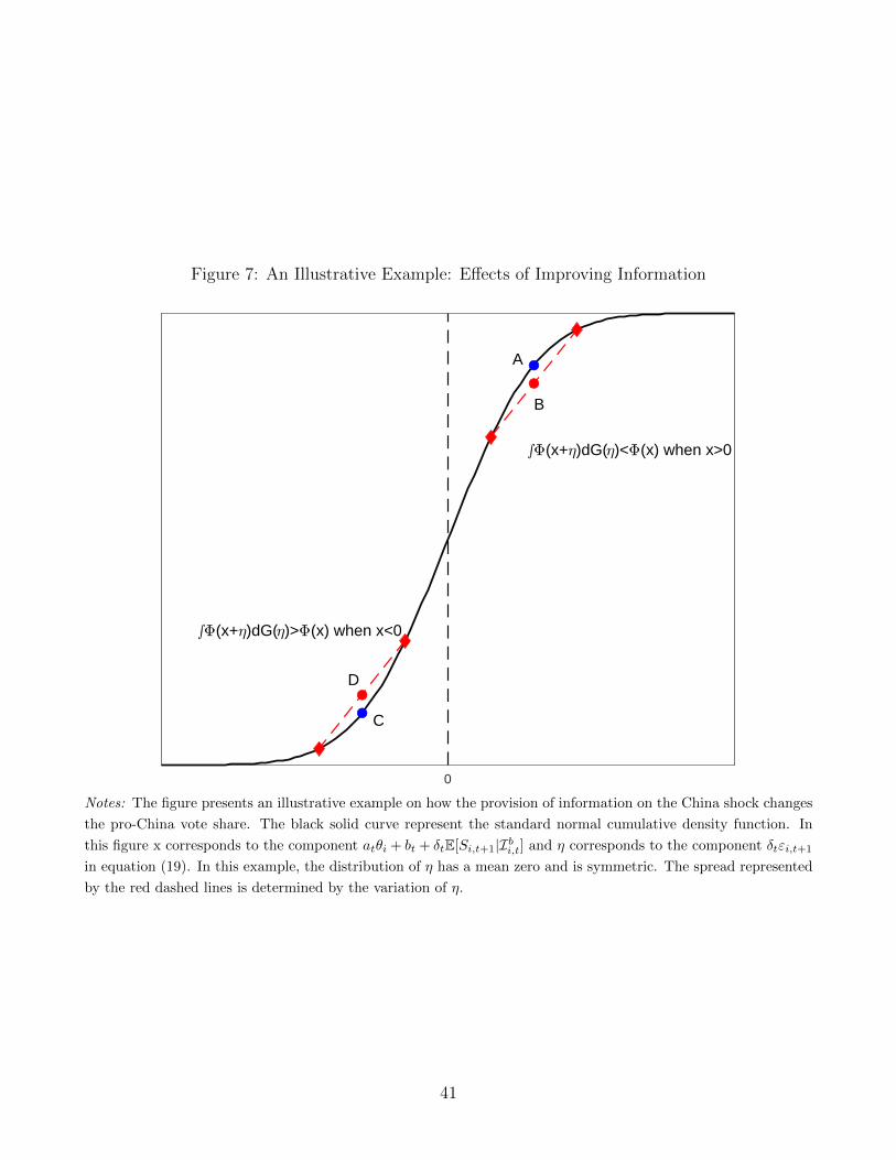
Figure 7: An Illustrative Example: Effects of Improving Information

0

(x+ )dG( )< (x) when x>0

(x+ )dG( )> (x) when x<0

A

B

C

D

Notes: The figure presents an illustrative example on how the provision of information on the China shock changes

the pro-China vote share. The black solid curve represent the standard normal cumulative density function. In

this figure x corresponds to the component atθi + bt + δtE[Si,t+1|Ibi,t] and η corresponds to the component δtεi,t+1

in equation (19). In this example, the distribution of η has a mean zero and is symmetric. The spread represented

by the red dashed lines is determined by the variation of η.

41

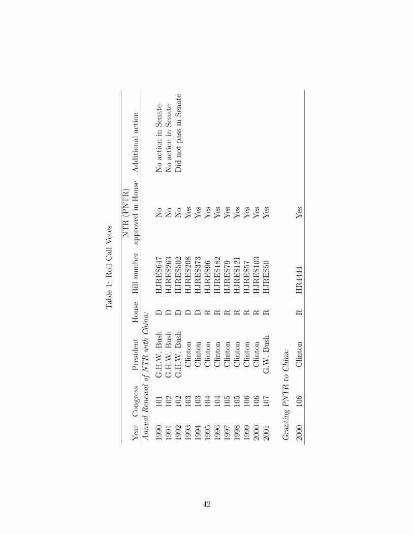
Tab

le1:

Rol

lC

all

Vot

es

NT

R(P

NT

R)

Yea

rC

ongr

ess

Pre

siden

tH

ouse

Bill

num

ber

appro

ved

inH

ouse

Addit

ional

acti

onA

nn

ual

Ren

ewal

ofN

TR

wit

hC

hin

a:

1990

101

G.H

.W.

Bush

DH

JR

ES64

7N

oN

oac

tion

inSen

ate

1991

102

G.H

.W.

Bush

DH

JR

ES26

3N

oN

oac

tion

inSen

ate

1992

102

G.H

.W.

Bush

DH

JR

ES50

2N

oD

idnot

pas

sin

Sen

ate

1993

103

Clinto

nD

HJR

ES20

8Y

es19

9410

3C

linto

nD

HJR

ES37

3Y

es19

9510

4C

linto

nR

HJR

ES96

Yes

1996

104

Clinto

nR

HJR

ES18

2Y

es19

9710

5C

linto

nR

HJR

ES79

Yes

1998

105

Clinto

nR

HJR

ES12

1Y

es19

9910

6C

linto

nR

HJR

ES57

Yes

2000

106

Clinto

nR

HJR

ES10

3Y

es20

0110

7G

.W.

Bush

RH

JR

ES50

Yes

GrantingPNTR

toChina:

2000

106

Clinto

nR

HR

4444

Yes

42

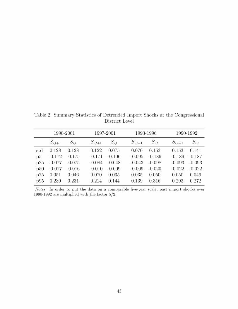
Table 2: Summary Statistics of Detrended Import Shocks at the CongressionalDistrict Level

1990-2001 1997-2001 1993-1996 1990-1992

Si,t+1 Si,t Si,t+1 Si,t Si,t+1 Si,t Si,t+1 Si,t

std 0.128 0.128 0.122 0.075 0.070 0.153 0.153 0.141p5 -0.172 -0.175 -0.171 -0.106 -0.095 -0.186 -0.189 -0.187p25 -0.077 -0.075 -0.084 -0.048 -0.043 -0.098 -0.093 -0.093p50 -0.017 -0.016 -0.010 -0.009 -0.009 -0.020 -0.022 -0.022p75 0.051 0.046 0.070 0.035 0.035 0.050 0.050 0.049p95 0.239 0.231 0.214 0.144 0.139 0.316 0.293 0.272

Notes: In order to put the data on a comparable five-year scale, past import shocks over1990-1992 are multiplied with the factor 5/2.

43

Tab

le3:

ML

EE

stim

ates

Bas

edon

Diff

eren

tIn

form

atio

nSet

s

a(s

e.)

b(s

e.)

δ(s

e.)

Pan

el

A:

1997-2

001

Min

imal

info

rmat

ionZi,t

=ShareMfg i,t,θi

0.65

0(0

.063

)0.

262

(0.0

25)

-0.8

10(0

.314

)B

asel

ine

info

rmat

ionZi,t

=S

i,t,ShareMfg i,t,θi

0.64

3(0

.062

)0.

263

(0.0

25)

-0.7

86(0

.279

)P

erfe

ctfo

resi

ght

0.61

9(0

.062

)0.

263

(0.0

25)

-0.0

18(0

.211

)

Pan

el

B:

1993-1

996

Min

imal

info

rmat

ionZi,t

=ShareMfg i,t,θi

-0.0

46(0

.084

)0.

678

(0.0

33)

-0.4

40(0

.611

)B

asel

ine

info

rmat

ionZi,t

=S

i,t,ShareMfg i,t,θi

-0.0

43(0

.084

)0.

679

(0.0

33)

-1.1

16(0

.549

)P

erfe

ctfo

resi

ght

-0.0

51(0

.083

)0.

678

(0.0

33)

-0.5

17(0

.452

)

Pan

el

C:

1990-1

992

Min

imal

info

rmat

ionZi,t

=ShareMfg i,t,θi

1.01

9(0

.104

)-0

.179

(0.0

37)

0.06

5(0

.351

)B

asel

ine

info

rmat

ionZi,t

=S

i,t,ShareMfg i,t,θi

1.00

0(0

.105

)-0

.181

(0.0

37)

-0.9

81(0

.288

)P

erfe

ctfo

resi

ght

1.01

3(0

.104

)-0

.180

(0.0

37)

-0.6

69(0

.244

)

Pan

el

D:

1990-2

001

Min

imal

info

rmat

ionZi,t

=ShareMfg i,t,θi

0.53

2(0

.044

)0.

280

(0.0

17)

-0.4

53(0

.222

)B

asel

ine

info

rmat

ionZi,t

=S

i,t,ShareMfg i,t,θi

0.53

4(0

.044

)0.

280

(0.0

17)

-0.8

56(0

.198

)P

erfe

ctfo

resi

ght

0.52

3(0

.044

)0.

280

(0.0

17)

-0.3

33(0

.147

)

Notes:

This

table

rep

orts

the

ML

Ees

tim

ate

sbas

edon

equat

ion

(6).

For

the

case

ofm

inim

al

info

rmat

ion,

we

repla

ceth

ete

rmE

[Si,t+

1|Ii,t]

by

the

pre

dic

ted

valu

eof

the

OL

Sre

gres

sion:Si,t+

1=β

0+β

1θ i

+β

2ShareMfg i,t

+ε i,t

+1.

For

the

case

ofbas

elin

ein

form

atio

n,

the

term

isre

pla

ced

by

the

pre

dic

ted

valu

eof

the

OL

Sre

gres

sion:Si,t+

1=

β0

+β

1θ i

+β

2ShareMfg i,t

+β

3Si,t

+ε i,t

+1.

For

the

case

ofp

erfe

ctfo

resi

ght,

the

term

isre

pla

ced

bySi,t+

1.

Rob

ust

stan

dar

der

rors

are

rep

orte

din

par

enth

eses

.

44

Table 4: Relevance of Manufacturing Employment Share and Past ImportShock in Explaining Future Import Shocks

Sample Period: 1990-2001 1997-2001 1993-1996 1990-1992Dependent Variable: Si,t+1 (1) (2) (3) (4)

Si,t 0.256*** 0.735*** 0.214*** 0.636***(0.011) (0.041) (0.013) (0.032)

ShareMfgi,t 0.753*** 0.683*** 0.455*** 0.695***(0.020) (0.036) (0.020) (0.045)

Observations 5,573 2,572 1,713 1,288R2 0.555 0.586 0.673 0.684

Notes: In order to put the data on a comparable five-year scale, past import shocks over1990-1992 are multiplied with the factor 5/2. Robust standard errors in parentheses. ***p<0.01, ** p<0.05, * p<0.1.

45

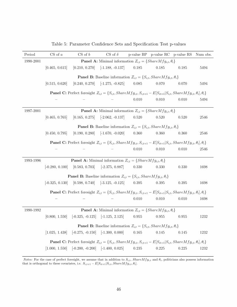
Table 5: Parameter Confidence Sets and Specification Test p-values

Period CS of a CS of b CS of δ p-value BP p-value RC p-value RS Num obs.

1990-2001 Panel A: Minimal information Zi,t = ShareMfgi,t, θi[0.465, 0.615] [0.210, 0.270] [-1.188, -0.137] 0.185 0.185 0.185 5494

Panel B: Baseline information Zi,t = Si,t, ShareMfgi,t, θi[0.515, 0.620] [0.240, 0.270] [-1.275, -0.825] 0.085 0.070 0.070 5494

Panel C: Perfect foresight Zi,t = Si,t, ShareMfgi,t, Si,t+1 − E[Sit+1|Si,t, ShareMfgi,t, θi], θi– – – 0.010 0.010 0.010 5494

1997-2001 Panel A: Minimal information Zi,t = ShareMfgi,t, θi[0.465, 0.765] [0.165, 0.275] [-2.062, -0.137] 0.520 0.520 0.520 2546

Panel B: Baseline information Zi,t = Si,t, ShareMfgi,t, θi[0.450, 0.795] [0.190, 0.280] [-1.670, -0.020] 0.360 0.360 0.360 2546

Panel C: Perfect foresight Zi,t = Si,t, ShareMfgi,t, Si,t+1 − E[Sit+1|Si,t, ShareMfgi,t, θi], θi– – – 0.010 0.010 0.010 2546

1993-1996 Panel A: Minimal information Zi,t = ShareMfgi,t, θi[-0.280, 0.100] [0.583, 0.703] [-2.375, 0.887] 0.330 0.330 0.330 1698

Panel B: Baseline information Zi,t = Si,t, ShareMfgi,t, θi[-0.325, 0.130] [0.598, 0.740] [-3.125, -0.125] 0.395 0.395 0.395 1698

Panel C: Perfect foresight Zi,t = Si,t, ShareMfgi,t, Si,t+1 − E[Sit+1|Si,t, ShareMfgi,t, θi], θi– – – 0.010 0.010 0.010 1698

1990-1992 Panel A: Minimal information Zi,t = ShareMfgi,t, θi[0.800, 1.550] [-0.325, -0.125] [-1.125, 2.125] 0.955 0.955 0.955 1232

Panel B: Baseline information Zi,t = Si,t, ShareMfgi,t, θi[1.025, 1.438] [-0.275, -0.150] [-1.300, 0.000] 0.165 0.145 0.145 1232

Panel C: Perfect foresight Zi,t = Si,t, ShareMfgi,t, Si,t+1 − E[Sit+1|Si,t, ShareMfgi,t, θi], θi[1.000, 1.550] [-0.200, -0.200] [-1.400, 0.025] 0.235 0.225 0.225 1232

Notes: For the case of perfect foresight, we assume that in addition to Si,t, ShareMfgi,t and θi, politicians also possess informationthat is orthogonal to these covariates, i.e. Si,t+1 − E[Sit+1|Si,t, ShareMfgi,t, θi].

46

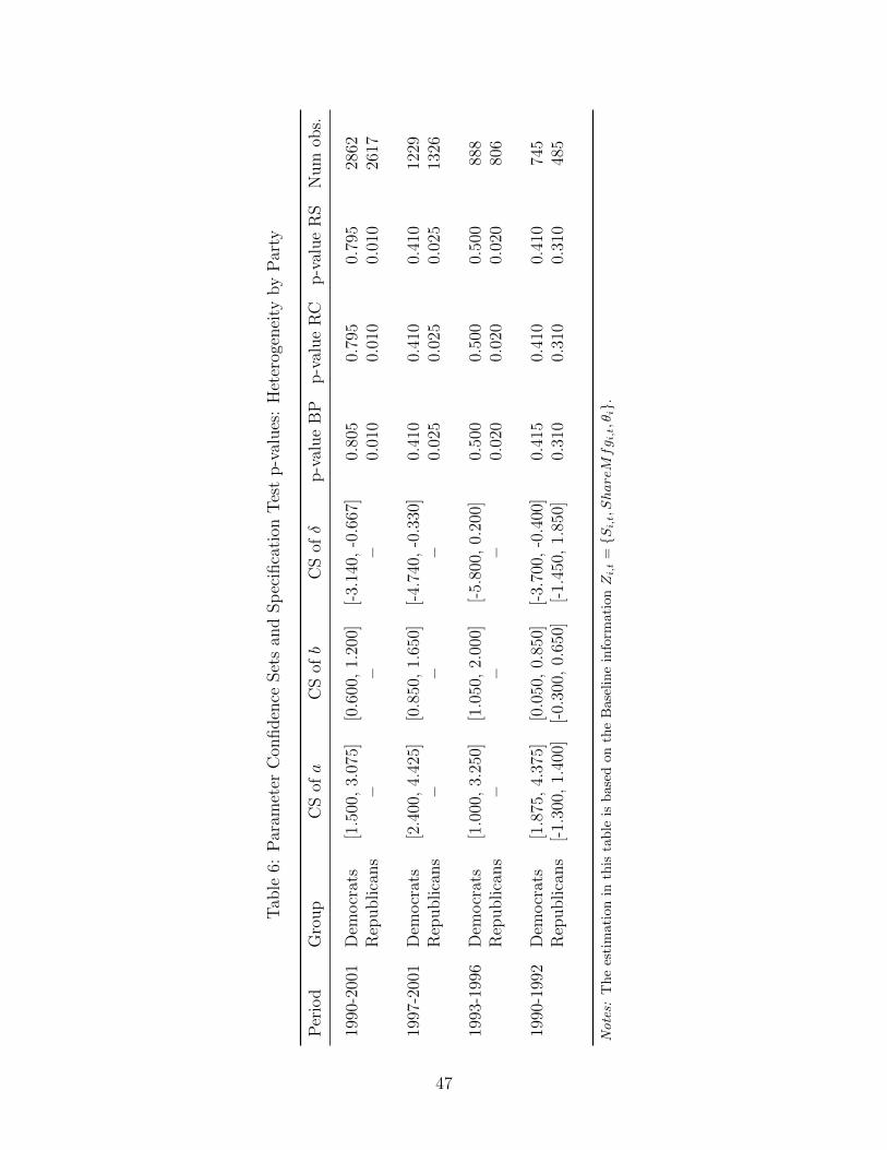
Tab

le6:

Par

amet

erC

onfiden

ceSet

san

dSp

ecifi

cati

onT

est

p-v

alues

:H

eter

ogen

eity

by

Par

ty

Per

iod

Gro

up

CS

ofa

CS

ofb

CS

ofδ

p-v

alue

BP

p-v

alue

RC

p-v

alue

RS

Num

obs.

1990

-200

1D

emocr

ats

[1.5

00,

3.07

5][0

.600

,1.

200]

[-3.

140,

-0.6

67]

0.80

50.

795

0.79

528

62R

epublica

ns

––

–0.

010

0.01

00.

010

2617

1997

-200

1D

emocr

ats

[2.4

00,

4.42

5][0

.850

,1.

650]

[-4.

740,

-0.3

30]

0.41

00.

410

0.41

012

29R

epublica

ns

––

–0.

025

0.02

50.

025

1326

1993

-199

6D

emocr

ats

[1.0

00,

3.25

0][1

.050

,2.

000]

[-5.

800,

0.20

0]0.

500

0.50

00.

500

888

Rep

ublica

ns

––

–0.

020

0.02

00.

020

806

1990

-199

2D

emocr

ats

[1.8

75,

4.37

5][0

.050

,0.

850]

[-3.

700,

-0.4

00]

0.41

50.

410

0.41

074

5R

epublica

ns

[-1.

300,

1.40

0][-

0.30

0,0.

650]

[-1.

450,

1.85

0]0.

310

0.31

00.

310

485

Notes:

The

esti

mat

ion

inth

ista

ble

isbas

edon

the

Bas

elin

ein

form

ati

onZi,t

=S

i,t,ShareMfg i,t,θi

.

47

Tab

le7:

Par

amet

erC

onfiden

ceSet

san

dSp

ecifi

cati

onT

est

p-v

alues

:H

eter

ogen

eity

by

Win

Mar

gin

Per

iod

Gro

up

CS

ofa

CS

ofb

CS

ofδ

p-v

alu

eB

Pp

-val

ue

RC

p-v

alu

eR

SN

um

obs.

1990

-200

1W

inm

argi

n>

med

ian

[0.6

00,

0.60

0][0

.150

,0.

200]

[-0.

555,

0.24

0]0.

115

0.11

50.

115

2551

Win

mar

gin<

med

ian

[0.1

50,

0.37

5][0

.300

,0.

400]

[-2.

495,

-0.8

82]

0.43

50.

435

0.43

525

51

1997

-200

1W

inm

argi

n>

med

ian

[0.8

25,

1.05

0][0

.075

,0.

275]

[-1.

985,

0.93

5]0.

685

0.68

50.

685

1182

Win

mar

gin<

med

ian

[0.1

50,

0.37

5][0

.250

,0.

375]

[-1.

905,

-0.1

73]

0.17

50.

175

0.17

511

84

1993

-199

6W

inm

argi

n>

med

ian

[-0.

250,

0.25

0][0

.475

,0.

700]

[-3.

000,

2.75

0]0.

525

0.52

00.

520

799

Win

mar

gin<

med

ian

[-1.

000,

0.25

0][0

.650

,0.

950]

[-8.

550,

-0.2

25]

0.95

00.

950

0.95

080

0

1990

-199

2W

inm

argi

n>

med

ian

[0.8

25,

2.10

0][-

0.45

0,-0

.100

][-

2.95

0,2.

650]

0.75

50.

755

0.75

556

8W

inm

argi

n<

med

ian

[0.4

50,

1.70

0][-

0.30

0,-0

.050

][-

4.37

5,-0

.750

]0.

495

0.48

50.

485

569

Notes:

Th

ees

tim

atio

nin

this

tab

leis

base

don

the

Bas

elin

ein

form

atio

nZi,t

=S

i,t,ShareMfg i,t,θi

.

48

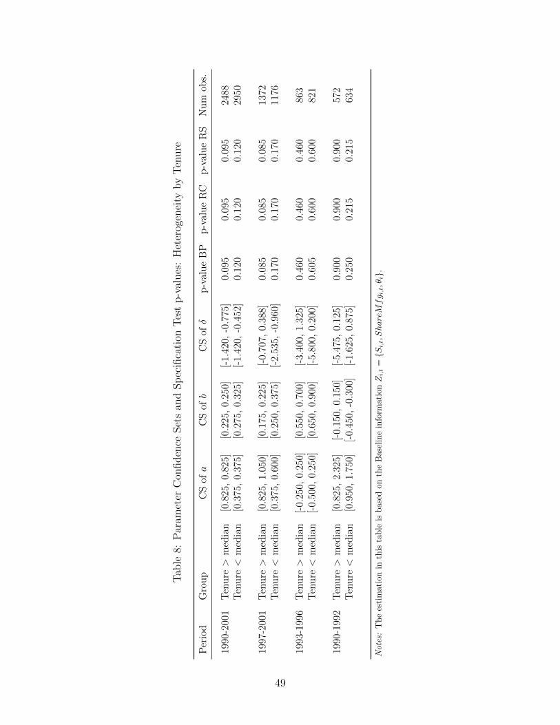
Tab

le8:

Par

amet

erC

onfiden

ceSet

san

dSp

ecifi

cati

onT

est

p-v

alues

:H

eter

ogen

eity

by

Ten

ure

Per

iod

Gro

up

CS

ofa

CS

ofb

CS

ofδ

p-v

alu

eB

Pp

-val

ue

RC

p-v

alu

eR

SN

um

obs.

1990

-200

1T

enu

re>

med

ian

[0.8

25,

0.82

5][0

.225

,0.

250]

[-1.

420,

-0.7

75]

0.09

50.

095

0.09

524

88T

enu

re<

med

ian

[0.3

75,

0.37

5][0

.275

,0.

325]

[-1.

420,

-0.4

52]

0.12

00.

120

0.12

029

50

1997

-200

1T

enu

re>

med

ian

[0.8

25,

1.05

0][0

.175

,0.

225]

[-0.

707,

0.38

8]0.

085

0.08

50.

085

1372

Ten

ure<

med

ian

[0.3

75,

0.60

0][0

.250

,0.

375]

[-2.

535,

-0.9

60]

0.17

00.

170

0.17

011

76

1993

-199

6T

enu

re>

med

ian

[-0.

250,

0.25

0][0

.550

,0.

700]

[-3.

400,

1.32

5]0.

460

0.46

00.

460

863

Ten

ure<

med

ian

[-0.

500,

0.25

0][0

.650

,0.

900]

[-5.

800,

0.20

0]0.

605

0.60

00.

600

821

1990

-199

2T

enu

re>

med

ian

[0.8

25,

2.32

5][-

0.15

0,0.

150]

[-5.

475,

0.12

5]0.

900

0.90

00.

900

572

Ten

ure<

med

ian

[0.9

50,

1.75

0][-

0.45

0,-0

.300

][-

1.62

5,0.

875]

0.25

00.

215

0.21

563

4

Notes:

The

esti

mat

ion

inth

ista

ble

isbas

edon

the

Bas

elin

ein

form

ati

onZi,t

=S

i,t,ShareMfg i,t,θi

.

49

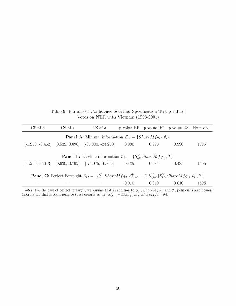
Table 9: Parameter Confidence Sets and Specification Test p-values:Votes on NTR with Vietnam (1998-2001)

CS of a CS of b CS of δ p-value BP p-value RC p-value RS Num obs.

Panel A: Minimal information Zi,t = ShareMfgi,t, θi[-1.250, -0.462] [0.532, 0.890] [-85.000, -23.250] 0.990 0.990 0.990 1595

Panel B: Baseline information Zi,t = SVi,t, ShareMfgi,t, θi[-1.250, -0.613] [0.630, 0.792] [-74.075, -6.700] 0.435 0.435 0.435 1595

Panel C: Perfect Foresight Zi,t = SVi,t, ShareMfgit, SVi,t+1 − E[SVi,t+1|SVi,t, ShareMfgi,t, θi], θi

– – – 0.010 0.010 0.010 1595

Notes: For the case of perfect foresight, we assume that in addition to Si,t, ShareMfgi,t and θi, politicians also possessinformation that is orthogonal to these covariates, i.e. SVi,t+1 − E[SVit+1|SVi,t, ShareMfgi,t, θi].

50

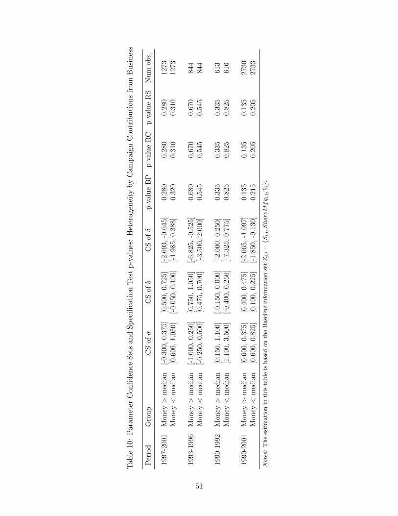
Tab

le10

:P

aram

eter

Con

fiden

ceSet

san

dSp

ecifi

cati

onT

est

p-v

alues

:H

eter

ogen

eity

by

Cam

pai

gnC

ontr

ibuti

ons

from

Busi

nes

s

Per

iod

Gro

up

CS

ofa

CS

ofb

CS

ofδ

p-v

alue

BP

p-v

alue

RC

p-v

alue

RS

Num

obs.

1997

-200

1M

oney

>m

edia

n[-

0.30

0,0.

375]

[0.5

00,

0.72

5][-

2.69

3,-0

.645

]0.

280

0.28

00.

280

1273

Mon

ey<

med

ian

[0.6

00,

1.05

0][-

0.05

0,0.

100]

[-1.

985,

0.38

8]0.

320

0.31

00.

310

1273

1993

-199

6M

oney

>m

edia

n[-

1.00

0,0.

250]

[0.7

50,

1.05

0][-

6.82

5,-0

.525

]0.

680

0.67

00.

670

844

Mon

ey<

med

ian

[-0.

250,

0.50

0][0

.475

,0.

700]

[-3.

500,

2.00

0]0.

545

0.54

50.

545

844

1990

-199

2M

oney

>m

edia

n[0

.150

,1.

100]

[-0.

150,

0.00

0][-

2.00

0,0.

250]

0.33

50.

335

0.33

561

3M

oney

<m

edia

n[1

.100

,3.

500]

[-0.

400,

0.25

0][-

7.32

5,0.

775]

0.82

50.

825

0.82

561

6

1990

-200

1M

oney

>m

edia

n[0

.600

,0.

375]

[0.4

00,

0.47

5][-

2.06

5,-1

.097

]0.

135

0.13

50.

135

2730

Mon

ey<

med

ian

[0.6

00,

0.82

5][0

.100

,0.

225]

[-1.

850,

-0.1

30]

0.21

50.

205

0.20

527

33

Notes:

Th

ees

tim

atio

nin

this

tab

leis

bas

edon

the

Bas

elin

ein

form

atio

nse

tZi,t

=S

i,t,ShareMfg i,t,θi

.

51

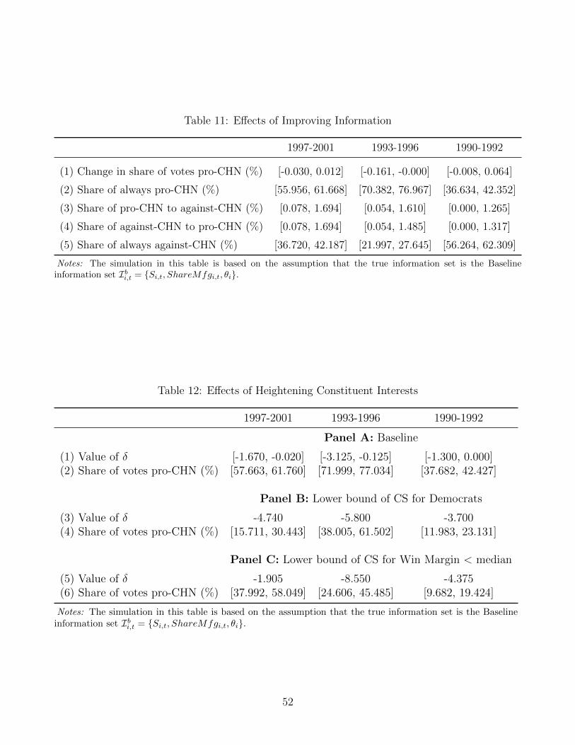
Table 11: Effects of Improving Information

1997-2001 1993-1996 1990-1992

(1) Change in share of votes pro-CHN (%) [-0.030, 0.012] [-0.161, -0.000] [-0.008, 0.064]

(2) Share of always pro-CHN (%) [55.956, 61.668] [70.382, 76.967] [36.634, 42.352]

(3) Share of pro-CHN to against-CHN (%) [0.078, 1.694] [0.054, 1.610] [0.000, 1.265]

(4) Share of against-CHN to pro-CHN (%) [0.078, 1.694] [0.054, 1.485] [0.000, 1.317]

(5) Share of always against-CHN (%) [36.720, 42.187] [21.997, 27.645] [56.264, 62.309]

Notes: The simulation in this table is based on the assumption that the true information set is the Baselineinformation set Ibi,t = Si,t, ShareMfgi,t, θi.

Table 12: Effects of Heightening Constituent Interests

1997-2001 1993-1996 1990-1992

Panel A: Baseline

(1) Value of δ [-1.670, -0.020] [-3.125, -0.125] [-1.300, 0.000](2) Share of votes pro-CHN (%) [57.663, 61.760] [71.999, 77.034] [37.682, 42.427]

Panel B: Lower bound of CS for Democrats

(3) Value of δ -4.740 -5.800 -3.700(4) Share of votes pro-CHN (%) [15.711, 30.443] [38.005, 61.502] [11.983, 23.131]

Panel C: Lower bound of CS for Win Margin < median

(5) Value of δ -1.905 -8.550 -4.375(6) Share of votes pro-CHN (%) [37.992, 58.049] [24.606, 45.485] [9.682, 19.424]

Notes: The simulation in this table is based on the assumption that the true information set is the Baselineinformation set Ibi,t = Si,t, ShareMfgi,t, θi.

52

Online Appendix

Not for Publication

53

A Data appendix and additional results

A.1 Other data

Roll call votes on NTR with Vietnam. We collect data on voting outcomes of bills related to

the renewal of Vietnam’s Jackson-Vanik Waiver (i.e., whether to extend Vietnam’s NTR status)

that existed over the period 1998 to 2002. Due to the congressional redistricting in 2002, we only

include the bills over 1998-2001. These bills are HJRES120, HJRES58, HJRES99 and HJRES55.

The share of votes in favor of NTR with Vietnam are 61.47%, 69.63%, 78.54% and 78.12% in 1998,

1999, 2000 and 2001, respectively.

Import shock from Vietnam. Analogous to the China shock, we construct the future

import supply shocks from Vietnam at the CZ level according to

SVj,t+1 =∑k

Ljk,tLj,t

∆M oth,Vk,t+1

Yk,t +Mk,t −Xk,t

,

where ∆M oth,Vk,t+1 is the change in import of good k from Vietnam by eight other (non-U.S.) high-

income countries over 5 years in the future. The past import shock from Vietnam is

SVj,t =∑k

Lik,t−5

Li,t−5

∆M oth,Vk,t

Yk,t−5 +Mk,t−5 −Xk,t−5

,

where ∆M oth,Vk,t denotes the change in import of good k from Vietnam by eight other (non-U.S.)

high-income countries over the past 5 years. We aggregate the CZ-level measures to congressional

districts using the same procedure in section 4.2. The CD-level measures are denoted by SVi,t+1

and SVi,t. The magnitude of the import shock from Vietnam is several orders smaller than that

from China. The standard deviation of SVi,t+1 over 1998-2001 is 0.0057. As with China, local man-

ufacturing share and past import shock have a large predicting power for future shock. Regressing

(de-trended) SVi,t+1 on (de-trended) SVi,t and ShareMfgi,t yields a R-squared of 0.528.

A.2 Evidence from congressional speech

The data on congressional speech is obtained from (Gentzkow et al., 2019). For each congressional

district×year cell, we count the number of speeches that refer “China” together with a mention of

trade issues or a mention of labor issues.36 The number of relevant speeches is related to import

36We identify the issues that each speech cover by keywords. The keywords for trade issues include trade,export/exports and import/imports. The keywords for labor issues include labor, employment, unemployment,and job/jobs.

54

shocks from China according to:

yit =∑c

βc1(t ∈ c)HighExposurei + γXit +Dt + εit, (A.1)

where yit is the number of speeches related to the “China and trade” issue or the “China and

labor” issue delivered by the representative of i in year t. Congressional districts are classified

into groups based on their exposure to the increase in China’s import penetration over the period

2001-2006. HighExposurei is an indicator variable equaling to 1 if i belongs to the top tercile of

the exposure to import shock from China. We allow its effect to vary across different congressional

sessions, and the differential effects are captured by coefficients βc. Xi represents the total number

of speeches delivered by the representative in district i and year t, and Dt denotes the year fixed

effects. Standard errors are clustered at the congressional district level.

Panel A of Figure A.1 reports the estimates of βc and the corresponding 90% confidence

intervals. The estimated coefficients become positively significant from the 107th congress (2001-

02) and on, when the China Shock over 2001 to 2006 gradually revealed itself. In contrast, the

estimates are smaller in magnitude and statistical insignificant over the earlier period 1989-1998.

In panels B and C, we estimate equation (A.1) for Democrats and Republicans separately. For

the purpose of comparison, y-axes in these two panels share the same scale. Two results emerge.

First, after the China Shock is realized, the representatives from the high-exposure districts raise

the related trade and labor issues more often in their speeches, but such response is stronger for

Democrats than Republicans. Second, it appears that Democrats started taking actions before

the China shock is realized. Specifically, for Democrats the estimated βc surged in 1999-2000

(i.e., the 106th congress), while for Republicans, the effect started picking up in 2001-2002. These

patterns are consistent with the findings in section 5 that (i) Democrats are more informed than

Republicans about the China shock before it was fully realized, and (ii) Democratic legislators

place more weights on the subconstituencies that would be adversely impacted by the future

import penetration from China.

55

Figure A.1: Number of Speeches with Mentions of China & Labor or China & Trade Issues

-.50

.51

Coe

ffici

ents

89-90

(101

)

91-92

(102

)

93-94

(103

)

95-96

(104

)

97-98

(105

)

99-00

(106

)

01-02

(107

)

03-04

(108

)

05-06

(109

)

07-08

(110

)

A. All Politicians

-.50

.51

1.5

Coe

ffici

ents

89-90

(101

)

91-92

(102

)

93-94

(103

)

95-96

(104

)

97-98

(105

)

99-00

(106

)

01-02

(107

)

03-04

(108

)

05-06

(109

)

07-08

(110

)

B. Democrats

-.50

.51

1.5

Coe

ffici

ents

89-90

(101

)

91-92

(102

)

93-94

(103

)

95-96

(104

)

97-98

(105

)

99-00

(106

)

01-02

(107

)

03-04

(108

)

05-06

(109

)

07-08

(110

)

C. Republicans

Notes: This figure plots the estimated coefficients βc in equation (A.1). Error bands show 90% confidence intervals.

Standard errors are clustered at the congressional district level. The vertical red dashed line indicates the time of

China’s accession to the WTO.

56

Tab

leA

.1:

Par

amet

erE

stim

ates

and

Con

tent

ofIn

form

atio

nSet

s(E

xte

nded

Model

:In

cludin

gC

ampai

gnC

ontr

ibuti

ons

from

Inte

rest

Gro

ups)

Per

iod

CS

ofa

CS

ofb

CS

ofδ

CS

ofχ

p-v

alu

eB

Pp

-val

ue

RC

p-v

alu

eR

SN

um

obs.

(Id

eolo

gy)

(Con

stan

t)(I

mp

ort

Sh

ock

)(M

oney

)

Pan

el

A:

Incl

ud

ing

Cam

paig

nC

ontr

ibu

tion

sfr

om

Bu

sin

ess

1997

-200

1[-

0.34

0,0.

940]

[0.2

67,

0.50

0][-

5.00

0,-0

.200

][0

.133

,0.

333]

0.82

50.

820

0.82

025

4619

93-1

996

[-1.

200,

0.00

0][0

.627

,0.

840]

[-8.

267,

1.06

7][0

.033

,0.

333]

0.73

00.

660

0.66

016

8819

90-1

992

[0.8

33,

1.43

3][-

0.23

3,-0

.133

][-

1.40

0,0.

000]

[0.0

00,

0.10

0]0.

110

0.10

00.

100

1229

Pan

el

B:

Incl

ud

ing

Cam

paig

nC

ontr

ibu

tion

sfr

om

Lab

or

1997

-200

1[-

0.70

0,0.

740]

[0.1

67,

0.26

7][-

1.93

3,-0

.067

][-

0.20

0,0.

000]

0.14

50.

145

0.14

525

4619

93-1

996

[-3.

667,

0.00

0][0

.307

,0.

893]

[-14

.733

,1.

733]

[-0.

600,

0.00

0]0.

750

0.69

00.

690

1688

1990

-199

2[-

4.00

0,5.

000]

[-0.

587,

0.20

7][-

7.00

0,5.

000]

[-0.

780,

0.66

0]0.

455

0.45

50.

455

1229

Pan

el

C:

Incl

ud

ing

the

2n

dP

rin

cip

al

Com

pon

ent

of

Cam

paig

nC

ontr

ibu

tion

sfr

om

Bu

sin

ess

an

dL

ab

or

1997

-200

1[-

2.91

3,-0

.273

][0

.100

,0.

600]

[-8.

133,

4.00

0][0

.667

,2.

167]

0.91

50.

900

0.90

025

4619

93-1

996

[-4.

667,

-0.6

67]

[0.4

40,

1.04

0][-

16.0

00,

6.00

0][0

.467

,2.

567]

0.60

50.

605

0.60

516

8819

90-1

992

[-4.

500,

0.30

0][-

0.50

0,0.

000]

[-6.

000,

-0.4

00]

[0.7

00,

3.03

3]0.

765

0.76

50.

765

1229

Notes:

The

esti

mat

ion

inth

ista

ble

isb

ased

onth

eas

sum

pti

on

that

the

info

rmat

ion

set

poss

esse

dby

pol

itic

ians

conta

insSi,t,ShareMfg i,t

,θ i

,and

the

cam

pai

gnco

ntr

ibu

tion

sfr

omth

eco

rres

pon

din

gin

tere

stgro

up

sd

uri

ng

the

con

gres

sion

alcy

cle.

57

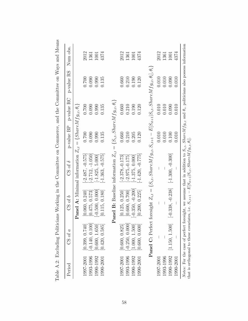
Tab

leA

.2:

Excl

udin

gP

olit

icia

ns

Wor

kin

gin

the

Com

mit

tee

onC

omm

erce

,an

dth

eC

omm

itte

eon

Way

san

dM

eans

Per

iod

CS

ofa

CS

ofb

CS

ofδ

p-v

alu

eB

Pp

-val

ue

RC

p-v

alu

eR

SN

um

obs.

Panel

A:

Min

imal

info

rmat

ionZi,t

=ShareMfg i,t,θi

1997

-200

1[0

.399

,0.

740]

[0.0

60,

0.24

0][-

2.48

7,-0

.575

]0.

700

0.70

00.

700

2012

1993

-199

6[-

0.14

0,0.

100]

[0.4

75,

0.57

3][-

2.71

2,-1

.050

]0.

090

0.09

00.

090

1361

1990

-199

2[0

.600

,1.

650]

[-0.

500,

0.00

0][-

1.82

5,5.

000]

0.99

00.

990

0.99

010

0119

90-2

001

[0.4

20,

0.58

5][0

.115

,0.

180]

[-1.

363,

-0.5

75]

0.13

50.

135

0.13

543

74

Panel

B:

Bas

elin

ein

form

atio

nZi,t

=S

i,t,ShareMfg i,t,θi

1997

-200

1[0

.600

,0.

825]

[0.1

25,

0.25

0][-

2.37

8,-0

.173

]0.

660

0.66

00.

660

2012

1993

-199

6[-

0.25

0,0.

000]

[0.6

00,

0.70

0][-

2.97

5,-0

.175

]0.

210

0.21

00.

210

1361

1990

-199

2[1

.000

,1.

500]

[-0.

350,

-0.2

00]

[-1.

375,

0.00

0]0.

205

0.19

00.

190

1001

1990

-200

1[0

.600

,0.

600]

[0.2

00,

0.22

5][-

1.42

0,-0

.775

]0.

120

0.12

00.

120

4374

Panel

C:

Per

fect

fore

sigh

tZi,t

=S

i,t,ShareMfg i,t,S

i,t+

1−E

[Sit

+1|Si,t,ShareMfg i,t,θi],θi

1997

-200

1–

––

0.01

00.

010

0.01

020

1219

93-1

996

––

–0.

010

0.01

00.

010

1361

1990

-199

2[1

.150

,1.

500]

[-0.

338,

-0.2

38]

[-1.

300,

-0.3

00]

0.10

00.

090

0.09

010

0119

90-2

001

––

–0.

010

0.01

00.

010

4374

Notes:

For

the

case

ofp

erfe

ctfo

resi

ght,

we

assu

me

that

inad

dit

ion

toSi,t,ShareMfg i,t

an

dθ i

,p

olit

icia

ns

als

op

oss

ess

info

rmati

on

that

isor

thog

onal

toth

ese

cova

riat

es,

i.e.Si,t+

1−E

[Sit

+1|Si,t,ShareMfg i,t,θi]

.

58

B Role of expectations about electoral sensitivity (γ)

Our baseline model assumes that politicians have full knowledge of the electoral consequences of

the China Shock that are dependent on the NTR voting decisions. In this appendix, we relax

this assumption. Denote γt = γ1t − γ2

t as the electoral sensitivity to the China Shock. Suppose

politicians form expectation on both γt and Si,t+1. Then the voting decision is determined by

Yi,t = 1atθi + bt + δE[γtSi,t+1|Ii,t]− ξi,t > 0.

The corresponding odds-based moment equality analogous to (8) is given by

E

[(1− Yi,t)

Φ(atθi + bt + δE[γtSi,t+1|Ii,t]

)1− Φ

(atθi + bt + δE[γtSi,t+1|Ii,t]

) − Yi,t∣∣∣∣∣Ii,t

]= 0. (B.1)

Here we make two assumptions: (i) γt and Si,t+1 are uncorrelated conditional on Iit, and (ii) the

distribution of γt conditional on Iit is equal to its distribution conditional on an information set

common to all politicians at time t, It. Under these assumptions we can rewrite (B.1) as:

E

[(1− Yi,t)

Φ(atθi + bt + δE [γt|It]E[Si,t+1|Ii,t]

)1− Φ

(atθi + bt + δE [γt|It]E[Si,t+1|Ii,t]

) − Yi,t∣∣∣∣∣Ii,t

]= 0

It is straightforward to redefine the coefficient δt = δE [γt|It] and reinterpret all the results we re-

port under this slightly different definition. We believe assumptions (i) and (ii) are not implausible

because the sensitivity of voting to economic shocks is a common parameter that does not depend

on the individual politician’s characteristics. We see γt as a parameter that politicians estimate

from voter surveys on the importance of certain issues in an election.37 The independence of the

China Shock from this parameter γt is also reasonable once we consider that this is a common

parameter that does not depend on specific constituencies.

C Monte Carlo simulation: MLE bias

In this Appendix, we adopt Monte Carlo simulations to illustrate the bias that emerges when

estimating ωt by maximum likelihood in equation (6). We adopt a time horizon of 5 years to

define a future import shock, so that Si,t+1 corresponds to the increase in import penetration

in the next 5 years. The true information set throughout the exercise is what we have defined

37See Jones and Baumgartner (2005).

59

as baseline information set Ibi,t = Sit,, ShareMfgi,t, θi. More specifically, Si,t+1 is simulated

according to the following linear model:

Si,t+1 = β0 + β1Si,t + β2ShareMfgi,t + β3θi︸ ︷︷ ︸E[Si,t+1|Ibi,t]

+εi,t+1,

where εi,t+1 is the expectational error. To simulate Si,t+1, we set β0 = 0, β1 = 0.721, β2 = 0.184,

β3 = 0. Expectational errors εi,t+1 are drawn from the normal distribution with mean 0 and

standard deviation of σε = 0.525.38 We take Si,t, ShareMfgi,t and θi from the real data over 1998-

2001. Then, the voting decision is simulated according to Yi,t = 1aθi+b+δE[Si,t+1|Ibi,t]−ξi,t > 0.We set a = 0.5 and b = 0.3 and present two sets of results based on δ = −1.3 and δ = 0.

We will evaluate the bias that arises when an econometrician mistakenly assumes that politi-

cians have minimal information Imi,t or perfect foresight Ipi,t. For the case of minimal information

set, we estimate ωt by maximizing the following log-likelihood:

lnL(ωt| Yi,t, θi, Ii,tNi=1

)(C.1)

=N∑i=1

Yi,t ln[Φ(atθi + bt + δtE

[Si,t+1|Imi,t

])]+ (1− Yi,t) ln

[1− Φ

(atθi + bt + δtE

[Si,t+1|Imi,t

])].

where the expectation is estimated as:

Si,t+1 = µ0 + µ1ShareMfgi,t + µ2θi︸ ︷︷ ︸E[Si,t+1|Imi,t]

+ui,t+1

For the case of perfect foresight the log-likelihood is maximized after replacing the expected future

shocks with Si,t+1.

Table C.1 reports the mean and the standard deviation of MLE estimates for 500 simulated

datasets. First, the simulations clearly indicate that when the model is correctly specified, the

average parameter estimates are very close to the true parameters. Second, when we assume the

politician has perfect foresight, i.e. more information than she actually does, there is a clear

attenuation bias. The average δ is -0.813 (the true δ is -1.3). We discussed the intuition for this

attenuation bias as related to classical measurement error in the main text. A more nuanced

case is the one in which the politician is assumed to have a Minimal information set, i.e. the

38The parameters β’s are estimated based on the actual data over 1998-2001. σε is set based on the empiricaldistribution of the regression residuals.

60

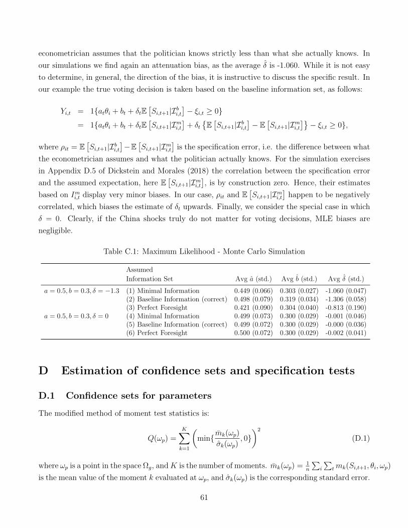
econometrician assumes that the politician knows strictly less than what she actually knows. In

our simulations we find again an attenuation bias, as the average δ is -1.060. While it is not easy

to determine, in general, the direction of the bias, it is instructive to discuss the specific result. In

our example the true voting decision is taken based on the baseline information set, as follows:

Yi,t = 1atθi + bt + δtE[Si,t+1|Ibi,t

]− ξi,t ≥ 0

= 1atθi + bt + δtE[Si,t+1|Imi,t

]+ δt

E[Si,t+1|Ibi,t

]− E

[Si,t+1|Imi,t

]− ξi,t ≥ 0,

where ρit = E[Si,t+1|Ibi,t

]−E

[Si,t+1|Imi,t

]is the specification error, i.e. the difference between what

the econometrician assumes and what the politician actually knows. For the simulation exercises

in Appendix D.5 of Dickstein and Morales (2018) the correlation between the specification error

and the assumed expectation, here E[Si,t+1|Imi,t

], is by construction zero. Hence, their estimates

based on Imi,t display very minor biases. In our case, ρit and E[Si,t+1|Imi,t

]happen to be negatively

correlated, which biases the estimate of δt upwards. Finally, we consider the special case in which

δ = 0. Clearly, if the China shocks truly do not matter for voting decisions, MLE biases are

negligible.

Table C.1: Maximum Likelihood - Monte Carlo Simulation

Assumed

Information Set Avg a (std.) Avg b (std.) Avg δ (std.)

a = 0.5, b = 0.3, δ = −1.3 (1) Minimal Information 0.449 (0.066) 0.303 (0.027) -1.060 (0.047)(2) Baseline Information (correct) 0.498 (0.079) 0.319 (0.034) -1.306 (0.058)(3) Perfect Foresight 0.421 (0.090) 0.304 (0.040) -0.813 (0.190)

a = 0.5, b = 0.3, δ = 0 (4) Minimal Information 0.499 (0.073) 0.300 (0.029) -0.001 (0.046)(5) Baseline Information (correct) 0.499 (0.072) 0.300 (0.029) -0.000 (0.036)(6) Perfect Foresight 0.500 (0.072) 0.300 (0.029) -0.002 (0.041)

D Estimation of confidence sets and specification tests

D.1 Confidence sets for parameters

The modified method of moment test statistics is:

Q(ωp) =K∑k=1

(minmk(ωp)

σk(ωp), 0)2

(D.1)

where ωp is a point in the space Ωg, andK is the number of moments. mk(ωp) = 1n

∑i

∑tmk(Si,t+1, θi, ωp)

is the mean value of the moment k evaluated at ωp, and σk(ωp) is the corresponding standard error.

61

When Q(ωp) = 0, it indicates that all the moment listed in (16) are satisfied at ωp, and hence

ωp could be included in the identified set. If Q(ωp) > 0, it indicates that some sample moment

inequalities are violated when evaluated at ωp. This may result from two independent cases: (i)

some population moment inequalities are indeed violated at ωp; and (ii) some sample moment

inequalities are violated because of sampling variation (Ho and Pakes, 2014).

To account for the sampling variation, we adopt the Generalized Moment Selection (GMS)

test in Andrews and Soares (2010) which simulates the asymptotic distribution of Q(ωp) under

the null hypothesis Ho : ω∗ = ωp. Here, ω∗ denotes the true parameter vector. More specifically,

the simulation is based on R draws from the multivariate normal distribution N(0K , IK), where

IK is the identity matrix of dimension K. Each draw ζr yields the following statistics:

QAAr (ωp) =

K∑k=1

((minΛ

12 (ωp)ζr]k, 0

)2

× 1√nmk(ωp)

σk(ωp)≤√

lnn)

(D.2)

where Λ(·) is the estimate of the variance-covariance matrix of mk(ωp)

σk(ωp). [Λ

12 (ωp)ζr]k is the kth

element of the vector Λ12 (ωp)ζr, and it is the simulated counterpart of mk(ωp)

σk(ωp)in equation (D.1).39

Pooling all QAAr (ωp) together renders the simulated distribution denoted by QAA(ωp).

Let cAA(ωp, 1 − α) denote the (1 − α)-quantile of QAA(ωp). ωp is included in the (1 − α)%

confidence set (CS) if Q(ωp) ≤ cAA(ωp, 1−α). By repeating the procedure for each point ωp in the

grid space Ωp, we derive the (1− α)% CS denoted by Ω1−α.40 In the main text, we set α = 0.05,

and report the 95% confidence sets.

D.2 BP, RC, and RS test statistics and corresponding p-values

This appendix details the statistical tests of whether covariates in Zi,t are contained in the infor-

mation set possessed by politicians when they vote on the NTR with China. Intuitively, when the

original voting model is correctly specified, but the information set is misspecified by researchers,

i.e Zi,t * Ii,t, some moment inequalities will be violated and the confidence set is likely to be

empty. In the following, we discuss the BP, RS and RS tests based on Bugni et al. (2015).

39The component 1√nmk(ωp)σk(ωp) ≤

√lnn is the generalized moment selection function which selects the moment

that are almost binding.40We conduct the grid search within a predefined grid space Ωg. If some of the points in Ω1−α are at the boundary

of Ωg, we expand the limits of the grid space and repeat the procedure described above. For our baseline model, wefill the 3-dimensional space with 64,000 equidistant grids. For the augmented model in section 5.5 and AppendixE.4, we fill the 4-dimensional space with 160,000 equidistant grids.

62

D.2.1 P-value of the Test BP

The test statistics for the Test BP is defined as in equation (D.1). For a given value of λ, we infer

whether ∀ ωp ∈ Ωg, Q(ωp) > cAA(ωp, 1− λ). If so, we lower λ by a small amount, and repeat the

procedure until reaching the value λBP such that ∃ ωp ∈ Ωg such that Q(ωp) ≤ cAA(ωp, 1− λBP ).

λBP is then the p-value for the test BP.41 As pointed out by Bugni et al. (2015), this test is too

conservative. Therefore, we turn to the test RC and the test RS proposed by the authors as

follows.

D.2.2 P-value of the Test RC

To conduct the test RC, we first calculate the minimum of test statistics (D.1) across all ωp ∈ Ωg.

Denote the minimum by T = minω∈Ωg

Q(ωp), and Ω∗g = arg minΩp

(Q(ωp)).42 The p-value of the test RC

is constructed as follows. For a given value of λ, we compute cRC(1− λ) = minωp∈Ω∗

g

cAA(ωp, 1− λ). If

T > cRC(1− λ), we lower λ by a small amount, and repeat the procedure until reaching the value

λRC such that T ≤ cRC(1− λRC). Then, λRC is the corresponding p-value.

D.2.3 P-value of the Test RS

Similar to the test RC, to conduct the test RS, we first compute T and derive Ω∗g as defined above.

Then, we use the R draws from the multivariate normal distribution N(0K , IK). For each draw ζr,

we compute QAAr (ωp) for each ωp ∈ Ω∗g according to equation (D.2), and derive the corresponding

minimum Tr = minωp∈Ω∗

g

QAAr (ωp). The p-value of the test RS is constructed as follows. For a given

value of λ, we find the (1 − λ)-quantile of Tr, denoted by cRS(1 − λ). If T > cRS(1 − λ), we

lower λ by a small amount, and repeat the procedure until reaching the value λRS such that

T ≤ cRS(1− λRS). Then, λRS is the corresponding p-value.

Note that the test RC and the test RS are different in the following way. For the test RC,

to derive the critical value cRC(1− λ), we first compute the (1− λ)-quantile for each asymptotic

distributions QAA evaluated at each ωp ∈ Ω∗g, and then take the minimum across these quantiles.

For the RS test, to derive the critical value cRS(1−λ), we first compute the minimum of QAAr (ωp)

across ωp ∈ Ω∗g, and then derive the (1− λ)-quantile of these minimums. When Ω∗g contains only

41In practice, we start the algorithm with λ = 0.99 and reduce it by 0.005 at a time. We stop when λ reaches0.01. Hence, p-value=0.01 (respectively, 0.99) in our tables indicates that the p-value is less than or equal to 0.01(respectively, greater than or equal to 0.99).

42As discussed in Ho and Pakes (2014) (pg. 3868), Ω∗g could be a set of values all of which make (D.1) zero(i.e., all the moments are satisfied), or it could be a point, indicating that no value of ω satisfies all the momentconditions. The latter case could be a result of sampling error, which is accounted for by the GMS approachproposed by Andrews and Soares (2010). In our case, Ω∗g contains only one point as the case in Ho and Pakes(2014).

63

one point, cRC(1− λ) = cRS(1− λ), and the p-values from the two tests are the same. When Ω∗g

contains multiple points, cRC(1−λ) ≥ cRS(1−λ), and the p-value of the test RS will be no larger

than that of the test RC.

E Further Robustness

E.1 Robustness to Violations of the Rational Expectation Assumption

Consider that the data generating process of future shock from China is

Si,t+1 = β0 + β1ShareMfgi,t + β2Si,t + εi,t+1, (E.1)

where E(εi,t+1|ShareMfgi,t, Si,t) = 0. In this exercise, we assume that Ii,t = θi, ShareMfgi,t, Si,t.

E.1.1 Case I: Expectational Errors Correlated with Si,t

Now, suppose that politicians form expectation in the following way:

E(Si,t+1|Ii,t) = β0 + β1ShareMfgi,t + (β2 + ρs)Si,t. (E.2)

When ρs < 0, it implies that politicians in the regions with a positive (respectively, negative) past

shock under-predict (respectively, over-predict) the future shock. The opposite is the case when

ρs > 0. The expectational error is then:

νi,t+1 = Si,t+1 − E(Si,t+1|Ii,t) = εi,t+1 − ρsSi,t.

In such scenario, the rational expectation assumption is violated, i.e., E(νi,t+1|Ii,t) 6= 0.

We infer the potential bias when the rational expectation assumption is violated by con-

ducting a Monte Carlo simulation as follows. First, we simulate the data on voting outcomes

based on the expected value in equation (E.2). Second, we then naively estimate our base-

line model. To simulate Si,t+1, we set β0 = 0, β1 = 0.721, β2 = 0.184. εi,t+1 are drawn

from the normal distribution with mean 0 and standard deviation of σε = 0.525. We take

Si,t, ShareMfgi,t and θi from the real data over 1998-2001, and simulate different cases with

ρs = −0.8,−0.6,−0.4,−0.2, 0, 0.2, 0.4, 0.6, 0.8. The deviation from the rational expectation as-

sumption is more severe the larger the absolute value of ρs is. Figure F.1 presents the estimated

confidence sets of the parameters a, b and δ corresponding to different ρs under Zi,t = Ii,t.There are four main findings. First, when ρs = 0 (i.e., the rational expectation assumption

holds), the 95% CS always contain the true parameters. Second, when ρs > 0, we find that (i)

64

confidence sets get wider for all parameters, and (ii) for δ, the CS shifts downward, and may not

cover the true value of δ when ρs is large enough. The intuition for (i) can be illustrated by the

mobl inequality. We start from the identity function

E

[(1− Yi,t)

Φ(atθi + bt + δtSi,t+1 − δtνi,t+1)

1− Φ(atθi + bt + δtSi,t+1 − δtνi,t+1)− Yi,t

∣∣∣∣∣Ii,t]

= 0. (E.3)

Setting aside the problem that vi,t+1 and Si,t+1 are correlated for now, a larger ρs increases the

variation of νi,t+1, which mechanically raises the left-hand-side of the following inequality and

hence reduces the obtained lower bounds:

E

[(1− Yi,t)

Φ(atθi + bt + δtSi,t+1)

1− Φ(atθi + bt + δtSi,t+1)− Yi,t

∣∣∣∣∣Ii,t]> 0.

A similar argument applies to inequalities mobu , mrp

l and mrpu . To glean some intuitions for (ii), we

note that when ρs > 0, vi,t+1 and Si,t+1 are negatively correlated. When we replace E(Si,t+1|Ii,t)by Si,t+1, the standard omitted variable bias problem drives the estimate of δ downward.

Third, when ρs < 0, we find that (i) confidence set of δ shits upward and may not cover the true

value of δ when ρs is negative enough, and (ii) the specification is rejected (i.e., the CS is empty)

when ρs = −0.8. On (i), the bias is induced by the similar omitted variable problem discussed

above. On (ii), it is because we set β2 = 0.721, and β2 +ρs ≈ 0 when ρs = −0.8. Note that in such

a case, Si,t takes little role in forming expectation on Si,t+1 (see equation E.2), and hence it is as if

politicians have no information on Si,t. (More precisely, it is as if politicians only have information

on θi, ShareMfgi,t, while researchers mistakenly assume Zi,t = θi, ShareMfgi,t, Si,t. Hence,

the specification is rejected.)

Fourth, even when ρs 6= 0, the confidence sets of a and b always contain the true values. This is

because in our data, the correlation between θi and Si,t is only 0.06. Therefore, an error correlated

with Si,t is unlikely to lead to a severe bias in the estimated coefficient for θi.

How likely are our baseline estimates of δ to be severely biased due to a violation of the rational

expectation assumption? Based on the simulated results in Figure F.1, the potential biases are

more concerning when |ρs| > 0.4. We also note that the standard deviation of εi,t+1 in equation

(E.1) is 0.525 (which is set to match the empirical distribution of the regression residuals), while

the standard deviation of Si,t is around 1. This implies that the standard deviation of ρsSi,t is

approximately ρs. In other words, the biases are more severe when the variation of irrational

expectational errors is at least as large as the variation of future China shock that is unexplained

by observables ShareMfgi,t and Si,t.

We now turn the attention to the case Zi,t 6⊆ Ii,t. Specifically, we use the simulated data with

65

different values of ρs, and estimate the model based on the assumption of perfect foresight. We

always reject the case of perfect foresight. In sum, it does not seem that the violation of rational

expectation assumption hinders our ability to reject the model with misspecified information set.

E.1.2 Case II: Expectational Errors Correlated with θi

We next consider the scenario in which the expectational errors are systematically correlated with

ideology. Specifically, the expectation of future China shock is given by

E(Si,t+1|Ii,t) = β0 + β1ShareMfgi,t + β2Si,t + ρθθi. (E.4)

The corresponding expectational error is

νi,t+1 = Si,t+1 − E(Si,t+1|Ii,t) = εi,t+1 − ρθθi.

When ρθ < 0, politicians with a positive (respectively, negative) θ under-predict (respectively,

over-predict) the future shock. This case implies that Republicans are more likely to under-predict

the future shock than Democrats. The opposite is the case when ρθ > 0. In such scenarios, the

rational expectation assumption is again violated, i.e., E(νi,t+1|Ii,t) 6= 0.

Based on the same parameterization of a, b, δ, σε, β0, β1, β2 as in section E.1.1 and the as-

sumption that Zi,t = Ii,t, we simulate data for different cases with ρθ = −1.6,−1.2,−0.8,−0.4,

0, 0.4, 0.8, 1.2, 1.6. The deviation from the rational expectation assumption is more severe the

larger the absolute value of ρθ is. Figure F.2 shows the estimated confidence sets of the parameters

a, b and δ corresponding to different ρθ under Zi,t = Ii,t.Two patterns emerge. First, the confidence sets are wide when ρθ is further away from 0.

Again, this is because the variation of νi,t+1 is larger when |ρθ| is larger. Second, the CS of a

shifts downward (respectively, upward) when ρθ becomes more positive (respectively, negative).

Specifically, when ρθ > 0, vi,t+1 = εi,t+1 − ρθθi and θi are negatively correlated. When we replace

E(Si,t+1|Ii,t) by Si,t+1 in the estimating equation, the standard omitted variable bias problem

drives the estimate of a downward. The opposite is the case when ρθ < 0.

Importantly, even when ρθ 6= 0, the confidence sets of b and δ always contain the true values.

Moreover, for the range of ρθ under consideration, we never reject the specification that politicians

have information on Zi,t = θi, ShareMfgi,t, Si,t. This is because in our data, the correlation

between θi and Si,t+1 is statistically zero, and the potential omitted variable correlated with θi has

little impact on estimating δ and inferring the information set. How severe is the bias associated

with the estimate of a? Based on the simulated results in Figure F.2, the potential biases are

more concerning when |ρθ| ≥ 1.2. In our data, the standard deviation of θi is 0.412. When

66

|ρθ| = 1.2, the standard deviation of ρθθi is 0.494, which is almost as large as the total variation

of future China shock that is unexplained by observables ShareMfgi,t and Si,t. Therefore, with

the presence of irrational expectational errors that are moderately correlated with ideology, the

baseline estimated CS of a is unlikely to be severely biased.

For a wide range of ρθ, we always reject the case of perfect foresight. Hence, the violation of

rational expectation assumption due to the correlation between expectational errors and ideology

does not seem to affect the power of the specification tests that we employ.

E.1.3 Case III: Expectation Error is a Non-Zero Constant

We now consider the case when all politicians under-predict (or over-predict) the China Shock

simultaneously. To probe this question, we simulate data assuming that the expectation on future

China shock conditional on Ii,t takes the following form:

E(Si,t+1|Ii,t) = β0 + ρ0 + β1ShareMfgi,t + β2Si,t. (E.5)

Hence, the expectational error in this case is

νi,t+1 = Si,t+1 − E(Si,t+1|Ii,t) = εi,t+1 − ρ0.

The rational expectation assumption is again violated, i.e., E(νi,t+1|Ii,t) 6= 0.

Figure F.3 presents the confidence sets for the simulated data for different cases with ρ0 =

−0.8,−0.6,−0.4,−0.2, 0, 0.2, 0.4, 0.6, 0.8. The simulation is based on the same parameterization

of a, b, δ, σε, β0, β1, β2 as in section E.1.1 and the assumption that Zi,t = Ii,t. Again, the absolute

value of ρ0 governs the extent to which the rational expectation assumption is violated. We find

that (i) the confidence sets are wider the larger is |ρ0|, and (ii) the confidence set of b shifts when

ρ0 6= 0, and does not cover the true value of b when |ρ0| gets larger.

Importantly, even when ρ0 6= 0, the confidence sets of a and δ always contain the true values.

Intuitively, this is analogous to the scenario that the OLS estimates other than the constant

coefficient remain consistent when the explanatory variable is changed by a constant. Since main

parameters of interest in our analysis are a and δ, we consider the case with ρ0 6= 0 less concerning.

As with aforementioned cases, we always reject the specification with perfect foresight. Hence,

the violation of rational expectation assumption due to a constant expectational error does not

seem to affect the power of the specification test.

67

E.2 Ideology-Dependent Information Sets

In this subsection, we simulate the data where politicians with θ ≤ 0 have access to information

on Ibi,t = θi, ShareMfgi,t, Si,t, while a share (π) of politicians with θ > 0 only have information

on Imi,t = θi, ShareMfgi,t. Their expectations on the future China Shock are rational, and are

given respectively by:

E(Si,t+1|Imi,t) = β0 + β1ShareMfgi,t + β2Si,t,

and

E(Si,t+1|Ibi,t) = β0 + β1ShareMfgi,t.

We simulate different cases with π = 0.5, 0.66, 0.75, 0.9, 1. We pool the data and test the

specification with baseline information set Ibi,t. Hence, the model is misspecified for some individ-

uals. Specifically, the case π = 1 is to capture the scenario that none of the Republicans have the

baseline information.

The results are reported in Figure F.4. We find that for the extreme case π = 1, the 95%

confidence set of δ is biased towards 0. The corresponding p-value of the RC test is 0.065. For

more realistic values of π (i.e, 0.5, 0.66 and 0.75), the CS of δ still covers the true value. In sum,

the estimation based on moment inequalities is largely robust to the case where the information

set is partially specified.

E.3 Import Shock including “NTR gap”

We consider an alternative measure that captures the potential impact on the electoral support

in commuting zone j if a politician voted in favor of China:

Sj,t+1 =∑k

Ljk,tLj,t

(NTRGapk,t ×

∆M othk,t+1

Yk,t +Mk,t −Xk,t

), (E.6)

where NTRGapk,t = ln(1 +NonNTR Tariffk,t)− ln(1 +NTR Tariffk,t). Specifically, the term

NTRGapk,t ×∆Moth

k,t+1

Yk,t+Mk,t−Xk,tis proportional to the potential reduction in the China shock at the

industry level if imports from China had faced the non-MFN tariffs. Therefore, ceteris paribus,

legislators are less likely to vote for China if the local economy specializes more in industries that

face larger supply shocks from China, but could receive more tariff protection if China’s NTR

status was revoked. The past shock is constructed analogously according to:

Sj,t =∑k

Ljk,t−5

Lj,t−5

(NTRGapk,t ×

∆M othk,t

Yk,t−5 +Mk,t−5 −Xk,t−5

). (E.7)

68

These the CZ level measures are then mapped to the CD level based on the procedure described

in the main text.

The correlation between the baseline measure and the alternative measure is 0.987 for the

future shock (Si,t+1) and 0.986 for the past shock (Si,t). The summary statistics of the alternative

measures described above are reported in Table F.1. Table F.2 repeats our baseline analysis using

the alternative measures (E.6) and (E.7). The results remains similar. Note that the estimate of

δ is larger in magnitude in Table. But it is due to the fact that the standard deviation of (E.6) is

about one third of the baseline measure.

E.4 Introducing Export Shocks

We construct the future export shock from China in CZ j according to:

SXj,t+1 =∑k

Ljk,tLj,t

∆Xothk,t+1

Yk,t +Mk,t −Xk,t

.

As with import shocks, we use the change in export of good k to China from eight other (non-U.S.)

high-income countries over 5 years in the future to capture the shift in export demand from China.

The past export shock are constructed accordingly. These the CZ level measures are then mapped

to the CD level based on the procedure in the main text.

In Table F.3, we augment the baseline model with export shocks. In the specification, we

assume Zi,t = Si,t, SXi,t, ShareMfgi,t, θi. The confidence sets get wider, and hence become less

informative. As is shown in Table F.4, past export shock is either uncorrelated (in 1997-2001) or

negatively correlated with future export shock (in 1993-1996, and 1990-1992). In addition, as is

reflected by the R-squared, the explanatory power of past export shock is weak especially in the

earlier period. This is in sharp contrast with findings related to the import shock – past import

shock is positively correlated with future shock, and together with local manufacturing employment

explains at least 55% of the variation in future shock. Hence, it appears that import shocks across

periods are more likely to reveal steady productivity growth in China, while export shock may

contain more time-varying idiosyncratic demand shocks. (At the industry-level, we find a negative

autocorrelation between past and future export shock over 1990-1999, the autocorrelation becomes

positive but statistically insignificant over 2000-2001.) Perhaps this partly explains why from the

reduced-form regression, we obtain a statistically insignificant effect of past export shock on voting

outcome. Specifically, using the data over 1990-2001, we regress a dummy variable indicating

voting in favor of China on past import shock, past export shock, manufacturing employment

share, ideology, and year dummies. The estimated coefficients (standard errors) are -0.401 (0.125),

-0.099 (0.103), 0.302 (0.257), and 0.183 (0.039), respectively.

69

To reduce the dimensionality of the model, we also consider a measure of future net import

shocks at CZ j as follows:

SNMj,t+1 =∑k

Ljk,tLj,t

∆M othk,t+1 −∆Xoth

k,t+1

Yk,t +Mk,t −Xk,t

.

The past net import shock are constructed accordingly. The CZ level measures are then mapped

to the CD level based on the procedure in the paper. Columns 1-4 of Table F.5 relate the future

net import shock SNMi,t+1 to the net past shock SNMi,t . We find that for the later periods, past net

import shock has weak predictive power on future shock. It is due to the fact that export shocks

are embedded in the net import measures, and the autocorrelation of export shocks is non-positive.

In columns (5)-(8), we regress the future net import shock SNMi,t+1 to the past import shock Si,t. It

is noted that import shock by itself has a significant predictive power.

Table F.6 employs the net import shock measure SNMi,t+1, and re-estimates the model. In light of

the findings in Table F.5, we assume Zi,t = Si,t, ShareMfgi,t, θi. The confidence sets are wider

compared to the baseline, but the results remain largely consistent with our main findings.

70

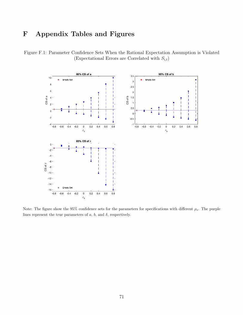
F Appendix Tables and Figures

Figure F.1: Parameter Confidence Sets When the Rational Expectation Assumption is Violated(Expectational Errors are Correlated with Si,t)

Note: The figure show the 95% confidence sets for the parameters for specifications with different ρs. The purple

lines represent the true parameters of a, b, and δ, respectively.

71

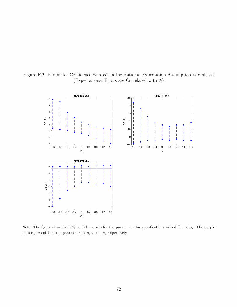
Figure F.2: Parameter Confidence Sets When the Rational Expectation Assumption is Violated(Expectational Errors are Correlated with θi)

Note: The figure show the 95% confidence sets for the parameters for specifications with different ρθ. The purple

lines represent the true parameters of a, b, and δ, respectively.

72

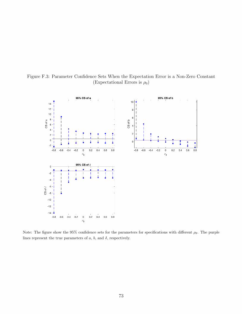
Figure F.3: Parameter Confidence Sets When the Expectation Error is a Non-Zero Constant(Expectational Errors is ρ0)

Note: The figure show the 95% confidence sets for the parameters for specifications with different ρθ. The purple

lines represent the true parameters of a, b, and δ, respectively.

73

Figure F.4: Parameter Confidence Sets When the Information Set is Misspecified for SomePoliticians with θ > 0

Note: The figure show the 95% confidence sets for the parameters for specifications with different ρθ. The purple

lines represent the true parameters of a, b, and δ, respectively.

74

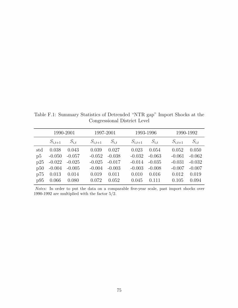
Table F.1: Summary Statistics of Detrended “NTR gap” Import Shocks at theCongressional District Level

1990-2001 1997-2001 1993-1996 1990-1992

Si,t+1 Si,t Si,t+1 Si,t Si,t+1 Si,t Si,t+1 Si,t

std 0.038 0.043 0.039 0.027 0.023 0.054 0.052 0.050p5 -0.050 -0.057 -0.052 -0.038 -0.032 -0.063 -0.061 -0.062p25 -0.022 -0.025 -0.025 -0.017 -0.014 -0.035 -0.031 -0.032p50 -0.004 -0.005 -0.004 -0.003 -0.003 -0.008 -0.007 -0.007p75 0.013 0.014 0.019 0.011 0.010 0.016 0.012 0.019p95 0.066 0.080 0.072 0.052 0.045 0.111 0.105 0.094

Notes: In order to put the data on a comparable five-year scale, past import shocks over1990-1992 are multiplied with the factor 5/2.

75

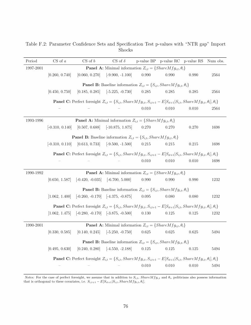
Table F.2: Parameter Confidence Sets and Specification Test p-values with “NTR gap” ImportShocks

Period CS of a CS of b CS of δ p-value BP p-value RC p-value RS Num obs.

1997-2001 Panel A: Minimal information Zi,t = ShareMfgi,t, θi[0.260, 0.740] [0.060, 0.270] [-9.900, -1.100] 0.990 0.990 0.990 2564

Panel B: Baseline information Zi,t = Si,t, ShareMfgi,t, θi[0.450, 0.750] [0.185, 0.285] [-5.225, -0.730] 0.285 0.285 0.285 2564

Panel C: Perfect foresight Zi,t = Si,t, ShareMfgi,t, Si,t+1 − E[Sit+1|Si,t, ShareMfgi,t, θi], θi– – – 0.010 0.010 0.010 2564

1993-1996 Panel A: Minimal information Zi,t = ShareMfgi,t, θi[-0.310, 0.140] [0.507, 0.688] [-10.875, 1.875] 0.270 0.270 0.270 1698

Panel B: Baseline information Zi,t = Si,t, ShareMfgi,t, θi[-0.310, 0.110] [0.613, 0.733] [-9.500, -1.500] 0.215 0.215 0.215 1698

Panel C: Perfect foresight Zi,t = Si,t, ShareMfgi,t, Si,t+1 − E[Sit+1|Si,t, ShareMfgi,t, θi], θi– – – 0.010 0.010 0.010 1698

1990-1992 Panel A: Minimal information Zi,t = ShareMfgi,t, θi[0.650, 1.587] [-0.420, -0.035] [-6.700, 5.000] 0.990 0.990 0.990 1232

Panel B: Baseline information Zi,t = Si,t, ShareMfgi,t, θi[1.062, 1.400] [-0.260, -0.170] [-4.375, -0.875] 0.095 0.080 0.080 1232

Panel C: Perfect foresight Zi,t = Si,t, ShareMfgi,t, Si,t+1 − E[Sit+1|Si,t, ShareMfgi,t, θi], θi[1.062, 1.475] [-0.280, -0.170] [-3.875, -0.500] 0.130 0.125 0.125 1232

1990-2001 Panel A: Minimal information Zi,t = ShareMfgi,t, θi[0.330, 0.585] [0.140, 0.245] [-5.250, -0.750] 0.625 0.625 0.625 5494

Panel B: Baseline information Zi,t = Si,t, ShareMfgi,t, θi[0.495, 0.630] [0.240, 0.280] [-4.550, -2.188] 0.125 0.125 0.125 5494

Panel C: Perfect foresight Zi,t = Si,t, ShareMfgi,t, Si,t+1 − E[Sit+1|Si,t, ShareMfgi,t, θi], θi– – – 0.010 0.010 0.010 5494

Notes: For the case of perfect foresight, we assume that in addition to Si,t, ShareMfgi,t and θi, politicians also possess informationthat is orthogonal to these covariates, i.e. Si,t+1 − E[Sit+1|Si,t, ShareMfgi,t, θi].

76

Tab

leF

.3:

Par

amet

erE

stim

ates

and

Con

tent

ofIn

form

atio

nSet

s:M

odel

Incl

udin

gE

xp

ort

Shock

s

Per

iod

CS

ofa

CS

ofb

CS

ofδ

CS

ofχ

p-v

alu

eB

Pp

-val

ue

RC

p-v

alu

eR

SN

um

obs.

(Id

eolo

gy)

(Con

stan

t)(I

mp

ort

Sh

ock

)(E

xp

ort

Sh

ock

)

1997

-200

1[-

1.27

3,1.

673]

[-0.

067,

0.60

0][-

10.7

00,

-3.5

67]

[2.5

33,

9.50

0]0.

990

0.99

00.

990

2564

1993

-199

6[-

0.82

0,0.

993]

[0.4

00,

0.90

0][-

11.2

00,

2.05

3][3

.067

,11

.500

]0.

990

0.99

00.

990

1698

1990

-199

2[-

1.50

0,2.

700]

[-0.

667,

0.16

7][-

10.4

00,

3.00

0][-

5.00

0,9.

300]

0.99

00.

990

0.99

012

3219

90-2

001

[-1.

200,

2.00

0][-

0.33

3,0.

667]

[-11

.800

,1.

080]

[2.6

13,

9.80

0]0.

990

0.99

00.

990

5494

Notes:

The

esti

mat

ion

inth

ista

ble

isbas

edon

the

ass

um

pti

on

that

the

info

rmat

ion

set

pos

sess

edby

politi

cian

sco

nta

insSi,t,SX i,t,ShareMfg i,t

,andθ i

.

77

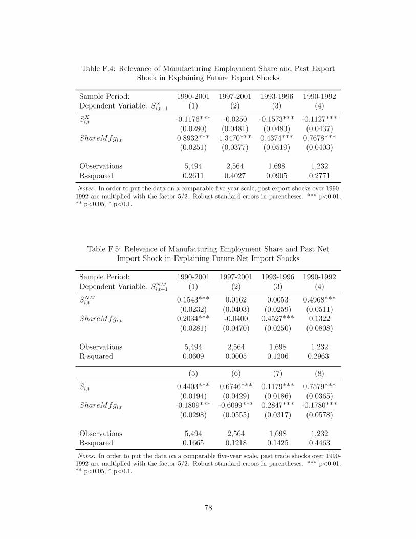
Table F.4: Relevance of Manufacturing Employment Share and Past ExportShock in Explaining Future Export Shocks

Sample Period: 1990-2001 1997-2001 1993-1996 1990-1992Dependent Variable: SXi,t+1 (1) (2) (3) (4)

SXi,t -0.1176*** -0.0250 -0.1573*** -0.1127***(0.0280) (0.0481) (0.0483) (0.0437)

ShareMfgi,t 0.8932*** 1.3470*** 0.4374*** 0.7678***(0.0251) (0.0377) (0.0519) (0.0403)

Observations 5,494 2,564 1,698 1,232R-squared 0.2611 0.4027 0.0905 0.2771

Notes: In order to put the data on a comparable five-year scale, past export shocks over 1990-1992 are multiplied with the factor 5/2. Robust standard errors in parentheses. *** p<0.01,** p<0.05, * p<0.1.

Table F.5: Relevance of Manufacturing Employment Share and Past NetImport Shock in Explaining Future Net Import Shocks

Sample Period: 1990-2001 1997-2001 1993-1996 1990-1992Dependent Variable: SNMi,t+1 (1) (2) (3) (4)

SNMi,t 0.1543*** 0.0162 0.0053 0.4968***(0.0232) (0.0403) (0.0259) (0.0511)

ShareMfgi,t 0.2034*** -0.0400 0.4527*** 0.1322(0.0281) (0.0470) (0.0250) (0.0808)

Observations 5,494 2,564 1,698 1,232R-squared 0.0609 0.0005 0.1206 0.2963

(5) (6) (7) (8)

Si,t 0.4403*** 0.6746*** 0.1179*** 0.7579***(0.0194) (0.0429) (0.0186) (0.0365)

ShareMfgi,t -0.1809*** -0.6099*** 0.2847*** -0.1780***(0.0298) (0.0555) (0.0317) (0.0578)

Observations 5,494 2,564 1,698 1,232R-squared 0.1665 0.1218 0.1425 0.4463

Notes: In order to put the data on a comparable five-year scale, past trade shocks over 1990-1992 are multiplied with the factor 5/2. Robust standard errors in parentheses. *** p<0.01,** p<0.05, * p<0.1.

78

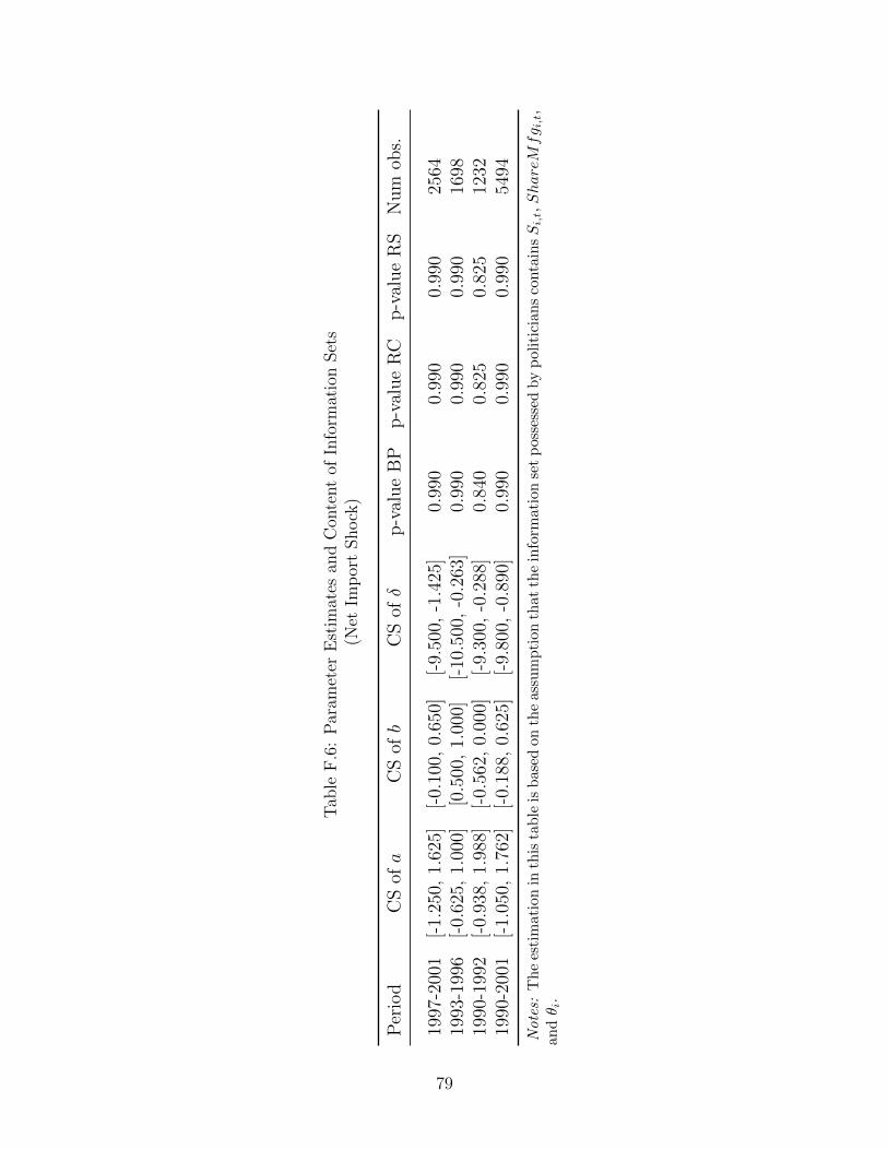
Tab

leF

.6:

Par

amet

erE

stim

ates

and

Con

tent

ofIn

form

atio

nSet

s(N

etIm

por

tShock

)

Per

iod

CS

ofa

CS

ofb

CS

ofδ

p-v

alue

BP

p-v

alue

RC

p-v

alue

RS

Num

obs.

1997

-200

1[-

1.25

0,1.

625]

[-0.

100,

0.65

0][-

9.50

0,-1

.425

]0.

990

0.99

00.

990

2564

1993

-199

6[-

0.62

5,1.

000]

[0.5

00,

1.00

0][-

10.5

00,

-0.2

63]

0.99

00.

990

0.99

016

9819

90-1

992

[-0.

938,

1.98

8][-

0.56

2,0.

000]

[-9.

300,

-0.2

88]

0.84

00.

825

0.82

512

3219

90-2

001

[-1.

050,

1.76

2][-

0.18

8,0.

625]

[-9.

800,

-0.8

90]

0.99

00.

990

0.99

054

94

Notes:

Th

ees

tim

atio

nin

this

tab

leis

bas

edon

the

ass

um

pti

on

that

the

info

rmati

on

set

poss

esse

dby

poli

tici

an

sco

nta

insSi,t,ShareMfg i,t

,an

dθ i

.

79