differential equations also known as engineering analysis or engiana

Differential Equations

Also known as

Engineering Analysis

or

ENGIANA

Introduction

In science, engineering, economics, and in most areas having a quantitative component, we are interested in describing how systems evolve in time, that is, in describing a system’s dynamics.

Introduction

• In this time series plot of a generic state function u = u(t) for a system, one can monitor the state of a system (e.g. population, concentration, temperature, etc) as a function of time.

• However, such curves or formulas tell us how a system behaves in time, but they do not give us insight into why a system behaves in the way we observe.

Introduction

• Thus, we try to formulate explanatory models that underpin the understanding we seek.

• Often these models are dynamic equations that relate the state u(t) to its rates of change, as expressed by its derivatives u′(t), u′′(t), ..., and so on.

Introduction

Before we present the formal definition, let’s see some examples of differential equations:

tsinqC

1'Rq

0sinl

g''

x''mx

K

p1rp'p

Introduction

The first equation models the angular deflections θ = θ(t) of a pendulum of length L.

0sinL

g''

Introduction

The second equation models the charge q = q(t) on a capacitor in an electrical circuit containing a resistor and a capacitor, where the current is driven by a sinusoidal electromotive force sin ωt operating at frequency ω.

tsinqC

1'Rq

Introduction

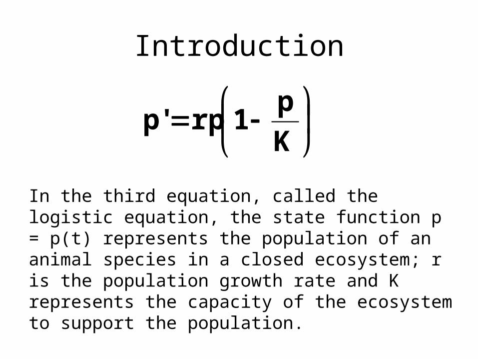
In the third equation, called the logistic equation, the state function p = p(t) represents the population of an animal species in a closed ecosystem; r is the population growth rate and K represents the capacity of the ecosystem to support the population.

K

p1rp'p

Introduction

The fourth equation represents a model of motion, where x = x(t) is the position of a mass acted upon by a force −αx.

x''mx

Introduction

• Differential Equation– An equation containing the derivatives of one

or more dependent variables, with respect to one or more independent variables, is said to be a differential equation (DE).

• Classification– By Type– By Order– By Linearity

Ordinary Differential Equations

• If an equation contains only ordinary derivatives of one or more dependent variables with respect to a single independent variable, it is said to be an ordinary differential equation (ODE).

xey5dx

dy

0y6dx

dy

dx

yd2

2

yx2dt

dy

dt

dx

Partial Differential Equations

• An equation involving partial derivatives of one or more dependent variables of two or more independent variables is called a partial differential equation (PDE).

x

v

y

u

0y

u

x

u2

2

2

2

t

u2

t

u

x

u2

2

2

2

Notation on ODEs

• Leibniz notation

• Prime notation

• Newton’s Dot Notation

32s32dt

sd2

2

.etc,dx

yd,

dx

yd,

dx

dy3

3

2

2

.etc,y,'''y,''y,'y )4(

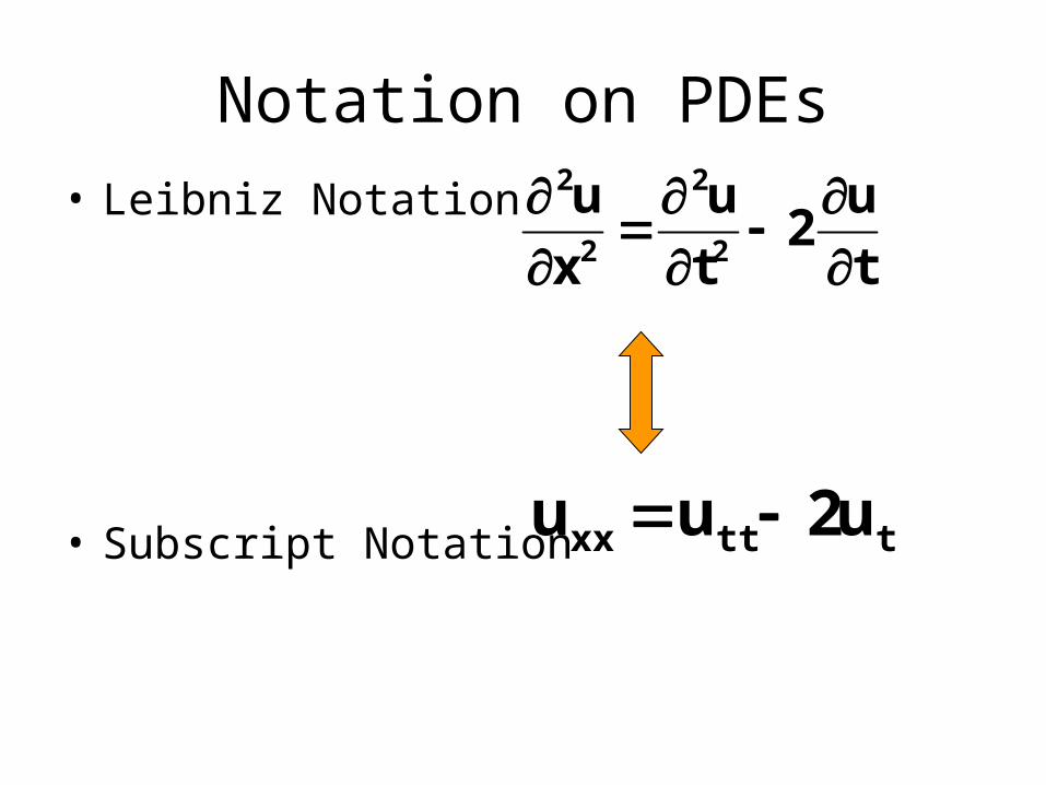
Notation on PDEs

• Leibniz Notation

• Subscript Notation tttxx u2uu

t

u2

t

u

x

u2

2

2

2

Order of a Differential Equation

• The order of a differential equation (either ODE or PDE) is the order of the highest derivative in the equation.

x

3

2

2

ey4dx

dy5

dx

yd

second order

Order of a Differential Equation

• The order of a differential equation (either ODE or PDE) is the order of the highest derivative in the equation.

yxdx

dyx4

first order

First Order ODEs

• First-order ordinary differential equations are occasionally written in the differential form M(x, y)dx + N(x, y)dy = 0.

• For example:

0xdy4dx)xy(

0xdy4dx)yx(

dx)yx(xdy4

yxdx

dyx4

General and Normal Forms of ODEs

• In symbols, we can express an nth-order ordinary differential equation in one dependent variable by the general form

where F is a real-valued function of n+2 variables x, y, y’, …, y(n).

0)y,...,''y,'y,y,x(F )n(


• In symbols, we can express an nth-order ordinary differential equation in one dependent variable by the normal form

where f is a real-valued continuous function.

)y,...,'y,y,x(fy

)y,...,'y,y,x(fdx

yd

)1n()n(

)1n(n

n


• Example of ODE in general form:

• Example of ODE in normal form:

0y6'y''y

y6'y''y

Linearity of ODEs

• An nth-order ordinary differential equation is said to be linear if F is linear in y, y’, …, y(n):

)x(gya'ya...yaya

)x(gy)x(adx

dy)x(a...

dx

yd)x(a

dx

yd)x(a

01)1n(

1n)n(

n

011n

1n

1nn

n

n

Linearity of ODEs

• First-order ODE:

• Second-order ODE:

)x(gya'ya

)x(gy)x(adx

dy)x(a

01

01

)x(gya'ya''ya

)x(gy)x(adx

dy)x(a

dx

yd)x(a

012

012

2

2

Linearity of ODEs

• The dependent variable y and all its derivatives y’, y’’, …, y(n), etc. are of the first degree (that is, the power of each said term involving y is 1).

• The coefficients a0, a1, …, an of y, y’,…,yn depend at most on the independent variable x.

)x(gya'ya...yaya

)x(gy)x(adx

dy)x(a...

dx

yd)x(a

dx

yd)x(a

011n

1nn

n

011n

1n

1nn

n

n

Linearity of ODEs• A linear, first order ODE:

• A linear, second order ODE

• A linear, third order ODE

0xdy4dx)xy(

x3

3

ey5dx

dyx

dx

yd

0y'y2''y

Nonlinear ODE

• A nonlinear ordinary differential equation is simply one that is not linear.

• Nonlinear functions of the dependent variable or its derivatives, such as sin(y) or ey’, cannot appear in a linear equation.

Nonlinear ODEs• A nonlinear, first order ODE:

• A nonlinear, second order ODE

• A nonlinear, fourth order ODE

xey2'y)y1(

0ydx

yd 24

4

0ysindx

yd2

2

Nonlinear term: coefficient depends

on y

Nonlinear term: nonlinear function

of y

Nonlinear term: power not 1

Nonlinear ODEs

A nonlinear ODE

0ydx

yd3

4

4

Nonlinear term: power not 1

Solution of an ODE

Any function , defined on an interval I and possessing at least n derivatives that are continuous on I, which when substituted into an nth-order ordinary differential equation reduces the equation to an identity, is said to be a solution of the equation on the interval.

Solution of an ODE

In other words, a solution of an nth-order ordinary differential equation is a function that possesses at least n derivatives and for which

for all x in I.

0))x(,...),x('),x(,x(F )n(

The Interval of the Solution

The Interval of the Solution is also called

– Interval of definition

– Interval of existence

– Interval of validity

– Domain of the solution

Solution Curve

• The graph of a solution of an ordinary differential equation is called a solution curve.

• Since is a differentiable function, it is continuous on its interval I of definition.

Families of Solutions

• The study of differential equations is similar to that of integral calculus.

• In some texts, a solution is sometimes referred to as an integral of the equation and its graph is called an integral curve.


• When evaluating an anti-derivative or indefinite integral in calculus, we use a single constant c of integration.

• Analogously, when solving a first-order differential equation F(x, y, y’) = 0, we usually obtain a solution containing a single arbitrary constant or parameter c.


• A solution containing an arbitrary constant represents a set G(x, y, c) = 0 of solutions called a one-parameter family of solutions.

• When solving an nth-order differential equation F(x, y, y’, …, y(n)) = 0, we seek an n-parameter family of solutions.– We integrate n times, hence we get n arbitrary

constants.


• This means that a single differential equation can possess an infinite number of solutions corresponding to the unlimited number of choices for the parameter(s).

• A solution of a differential equation that is free of arbitrary parameters is called a particular solution.


For example, the one-parameter family

y = cx – xcosx

is a solution of the linear first-order equation

xy’ – y = x2sinx

on the interval (-, ).


Check:

y = cx – xcosx

y’ = c – ( cosx + x(-sinx) )

y’ = c – cosx + xsinx

xy’ – y = x2sinx

x(c – cosx + xsinx) – (cx – xcosx) = x2sinx

cx – xcosx + x2sinx – cx + xcosx = x2sinx

x2sinx = x2sinx


Some solutions of xy’ – y = x2sinx

Graph of y = cx – xcosx


If every solution of an nth-order ODE F(x, y, y’, …, y(n)) on an interval I can be obtained from an n-parameter family G(x, y, c1, c2, …, cn) = 0 by appropriate choices of the parameters ci, i = 1, 2, …, n, we then say that the family is the general solution of the differential equation.

Singular Solution

• Sometimes a differential equation possesses a solution that is not a member of a family of solutions of the equation – that is, a solution that cannot be obtained by specializing any of the parameters in the family of solutions.

• Such an extra solution is called a singular solution.

Singular Solution

For example,

is a solution of the differential equation

on the interval (-, ).

2

2 cx4

1y

2

1

xydx

dy

Singular Solution

When c = 0, the resulting particular solution is

But notice that the trivial solution y = 0 is a singular solution, since it is not a member of the family y = (1/2x2 + c)2; there is no way of assigning a value to the constant c to obtain y = 0.

4x16

1y

Initial-Value Problems (IVPs)

We are often interested in problems in which we seek a solution y(x) of a differential equation so that y(x) satisfies prescribed side conditions – that is, conditions imposed on the unknown y(x) or its derivatives.


Solve:

Subject to:

where y0, y1, …, yn-1 are arbitrarily specified real constants.

)y...,,'y,y,x(fdx

yd )1n(n

n

1n0)1n(

10

00

y)x(y

y)x('y

y)x(y


• Such a problem is called an initial-value problem (IVP).

• The values of y(x) and its first n-1 derivatives at single point x0 (i.e., y(x0) = y0, y’(x0) = y1, …, y(n-1)(x0) = yn-1) are called initial conditions.

First-Order IVP

)y,x(fdx

dy

00 y)x(y

Solve:

Subject to:

Second-Order IVP

)'y,y,x(fdx

yd2

2

10

00

y)x('y

y)x(y

Solve:

Subject to: m = y1

Example

What function do you know from calculus is such that its first derivative is itself?

Example

• Answer: y = Cex

• y = Cex

so that

y’ = Cex

and hence,

y = y’

• If we impose the following initial condition

y(0) = 3

then we have

y = Cex

3 = Ce0

3 = C

Example

• Hence, y = 3ex is a solution of the IVP

y’ = y

y(0) = 3

• If we impose the following initial condition

y(1) = -2

then we have

y = Cex

-2 = Ce1

-2/e = C

Example

• Hence,

y = (-2/e)ex or

y = -2ex-1

is a solution of the IVP

y’ = y

y(1) = -2

• The two solution curves are shown in dark blue and dark red in the next figure.

Example

The solution curves for

and

3)0(y

'yy

2)1(y

'yy

Existence of a Unique Solution

Theorem

Let R be a rectangular region in the xy-plane defined by a x b, c y d that contains the point (x0, y0) in its interior. If f(x, y) and ∂f/∂y are continuous on R, then there exist some interval I0: (xo - h, xo + h), h > 0, contained in [a, b], and a unique function y(x), defined on I0, that is a solution of the initial-value problem.

Existence of a Unique Solution

Direction or Slope Fields

• Recall that a derivative dy/dx of a differentiable function y = y(x) gives slopes of tangent lines at points on its graph.

• The derivative itself is also a function. In other words,

)y,x(fdx

dy


• The function f in the normal form is called the slope function or rate function.

• The value f(x,y) that the function f assigns to a point (x,y) represents the slope of a line; alternatively, we can envision it as a line segment called a lineal element.


• For example, say we’re given the following function f and a point (2, 3) on the solution curve:

• At the point (2, 3), the slope of a lineal element is f(2,3) = 2(2)(3) = 1.2.

)3,2(

xy2.0)y,x(fdx

dy

A lineal element at a point A lineal element is tangent to the solution curve that passes through the point

in consideration


If we systematically evaluate f over a rectangular grid of points in the xy plane and draw a line element at each point (x,y) of the grid with slope f(x,y), then the collection of all these lines is called a direction field or a slope field of the differential equation dy/dx = f(x,y).


Visually, the direction field suggests the appearance or shape of a family of solution curves of the differential equation, and consequently, it may be possible to see at a glance certain qualitative aspects of the solutions.

A single solution curve that passes through a direction field must follow the flow pattern of the

field. It is tangent to a line element when it intersects a point

in the grid. This figure shows a computer

generated direction field of dy/dx = sin(x+y) over a region of the xy

plane. Note how the solution curves shown in color follow the

flow of the field.


Going back to

it can be shown that

is a one-parameter family of solutions.

xy2.0)y,x(fdx

dy

2x1.0cey

Direction Field for dy/dx = 0.2xy

Some solution curves in the family

2x1.0cey

Solving Differential Equations

1. Analytical Approach

2. Qualitative Approach

3. Numerical Approach


1. Analytical Approach

– Exact solution using mathematical principles (calculus)

– Main focus of this course (ENGIANA)


2. Qualitative Approach– Gleaning from the differential

equation answers to questions such as

• Does the DE actually have solutions?

• If a solution of the DE exists and satisfies an initial condition, is it the only such solution?

• What are some of the properties of the unknown solutions?

• What can we say about the geometry of the solution curves?


3. Numerical Approach– Use of numerical

methods and computer algorithms• Can we somehow

approximate the values of an unknown solution?

differential equations also known as engineering analysis or engiana

Documents