differential equations ordinary differential equations exponential growth or decay families of...

Differential Equations

Ordinary Differential EquationsExponential Growth or DecayFamilies of SolutionsSeparation of VariablesNumerical Solving – Direction FieldsHybrid Numerical-Symbolic SolvingOrthogonal CurvesModeling

Mika Seppälä: Differential Equations

Ordinary Differential Equations

4 2 2 3sin , ' 2 0, 0y x y y xy x y y x

Definition A differential equation is an equation involving derivatives of an unknown function and possibly the function itself as well as the independent variable.

Example

Definition The order of a differential equation is the highest order of the derivatives of the unknown function appearing in the equation

1st order equations 2nd order equation

sin cosy x y x CExamples 2 3

1 1 26 e 3 e ex x xy x y x C y x C x C

In the simplest cases, equations may be solved by direct integration.

Observe that the set of solutions to the above 1st order equation has 1 parameter, while the solutions to the above 2nd order equation depend on two parameters.


Exponential Growth or Decay

dy

kdty

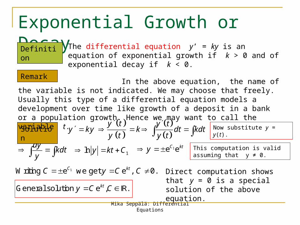
Definition The differential equation y’ = ky is an equation of exponential growth if k > 0 and of exponential decay if k < 0.

Remark

y ty ky k

y t

Solution

y t

dt kdty t

In the above equation, the name of the variable is not indicated. We may choose that freely. Usually this type of a differential equation models a development over time like growth of a deposit in a bank or a population growth. Hence we may want to call the variable t.

Now substitute y = y(t).

1ln y kt C 1e eC kty

1Writing e we get e , 0.C ktC y C C

This computation is valid assuming that y ≠ 0.

Direct computation shows that y = 0 is a special solution of the above equation. General solution e , .kty C C


Families of Solutions 9 ' 4 0yy x

1 19 ' 4 9 ( ) '( ) 4yy x dx C y x y x dx xdx C

2 21This yields where .

4 9 18

Cy xC C

Example

Solution

The solution is a family of ellipses.

2

2 2 2 21 1 1

99 2 2 9 4 2

2

yydy x C x C y x C

Observe that given any point (x0,y0), there is a unique solution curve of the above equation which curve goes through the given point.


Separation of Variables

and are separable

but is not separable.

xy xy y

y

x yy

x y

Definition A differential equation of the type y’ = f(x)g(y) is separable.

Example

x

y y x y x xy

Example y x y x dx xdx

Separable differential equations can often be solved with direct integration. This may lead to an equation which defines the solution implicitly rather than directly.

2 2

2 212 2

y xC y x C ydy xdx

Substitute y = y(x) to simplify this integral.



x

y y x y x xy

Example

2 2

2 212 2

y xC y x C

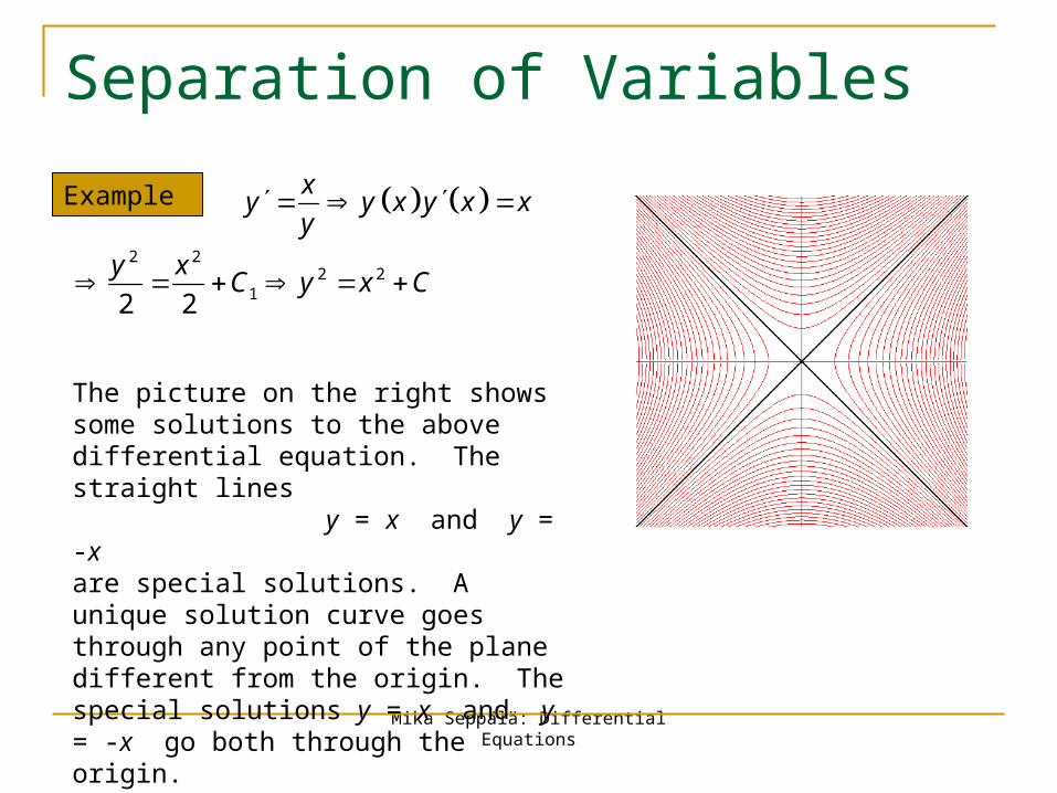
The picture on the right shows some solutions to the above differential equation. The straight lines y = x and y = -x are special solutions. A unique solution curve goes through any point of the plane different from the origin. The special solutions y = x and y = -x go both through the origin.


General Separable Equations

f g f

g

y xy x x y x x

y x

g f

dy dx

y x

f

g

y xdx x dx

y x

Consider the separable equation y’ = f(x) g(y).

This computation is valid provided that g(y) ≠ 0.

Observe that if y0 is such that g(y0)=0, then the constant function y = y0 is a solution to the above differential equation. Hence all solutions to the equation g(y) = 0 give special solutions to the above differential equation.

We get:

Substitute y = y(x).

If integration can be performed, this usually leads to an equation that defines y implicitly as a function of x.



2

2

x xy

y yExample

2 2

2 2

x x dy x xy

y y dx y ySolution 2 2y y dy x x dx

3 2 3 212 3 2 3 6y y x x C

3 2 3 2

13 2 3 2

y y x xC

3 2 3 212 3 2 3 , where 6 .y y x x C C C

This notation is due to Leibniz.

It is, in principle, possible to solve y in terms of x and C from the above implicit solution. This would lead to very long expressions. The picture on the right shows some solution curves.


Numerical SolvingSolutions to a differential equation of the type y’ = f(x,y) can always be approximated numerically by computing the direction field or the slope field defined by this equation.

The computation has the following steps:

1. Choose first a rectangle in the xy-plane in which rectangle you want to approximate solutions.

2. Form a grid of points of the rectangle. Choose the points so that they cover the rectangle in question evenly.

3. At each grid point (x,y) compute the value of the function f(x,y).

4. Starting from each grid point draw a short arrow with slope f(x,y).

5. Connect arrows to form an approximation of a solution curve.


Numerical Solving

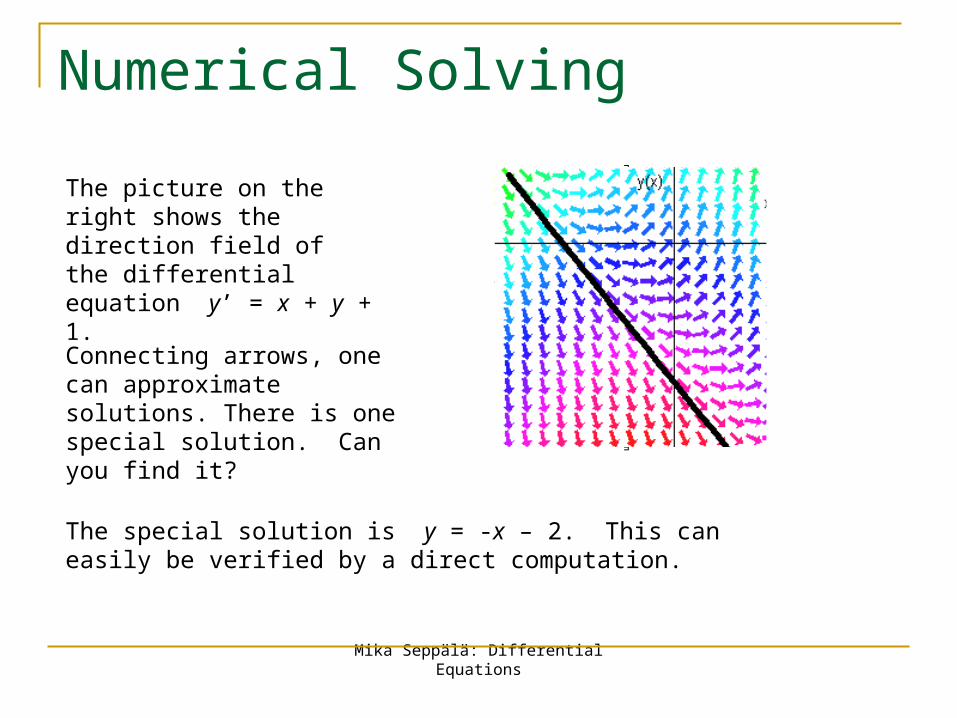
The picture on the right shows the direction field of the differential equation y’ = x + y + 1.

Connecting arrows, one can approximate solutions. There is one special solution. Can you find it?

The special solution is y = -x – 2. This can easily be verified by a direct computation.


Hybrid Numerical-Symbolic SolvingBy plotting the direction field of the differential equation y’ = x + y +1 we found the special solution y = -x - 2.

To find the general solution, substitute y = -x - 2 + v to the original equation and solve for v (which is a new unknown function).

One gets y’ = -1 + v’ and the equation for v is -1 + v’ = x + (-x -2 + v) + 1.

This simplifies to v’ = v which can be solved by direct integration.

dv dv dvv dx dx

dx v v 1

1ln e e e .C x xv x C v C

The general solution is y = -x – 2 + Cex.Conclusion


Orthogonal Curves (1)

By differentiation we get: ' 2 . Hence the family of parabola

in question satisfies the differential equation ' 2 .

y x

y x

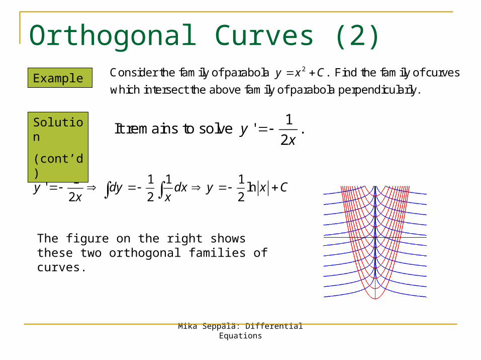
2Consider the family of parabola . Find the family of curves

which intersect the above family of parabola perpendicularly.

y x C Example

Solution

Two curve intersect perpendicularly if the product of the slopes of the tangents at the intersection point is -1. This gives the following differential equation for the orthogonal family of curves.

1'

2y

x


Orthogonal Curves (2)

1 1 1 1' ln

2 2 2y dy dx y x C

x x

1It remains to solve ' .

2y

x

2Consider the family of parabola . Find the family of curves

which intersect the above family of parabola perpendicularly.

y x C Example

Solution

(cont’d)

The figure on the right shows these two orthogonal families of curves.


Newton’s Law of Heating and Cooling

Newton’s Law The temperature of a hot or a cold object decreases or increases at a rate proportional to the difference of the temperature of the object and that of its surrounding.

Let H(t) be the temperature of the hot or cold object at time t. Let H∞ be the temperature of the surrounding. With this notation Newton’s Law can be expressed as the differential equation

H’(t) = k (H(t)- H∞).

In Leibniz’s notation:

HH H .

dk

dt

The unknown coefficient k must be determined experimentally.


Cooking a TurkeyExample

Solution

A turkey is put in a oven heated to 300 degrees (F). Initially the temperature of the turkey is 70 degrees. After one hour the temperature is 86 degrees. How long does it take until the temperature of the turkey is 180 degrees?

The differential equation is H’ = k (H – 300).

H HH 300

H 300d d

k k dtdt

1

Hln H 300

H 300d

k dt kt C

1H 300 e e H 300 e .C kt ktC

Here the coefficient C may take any value including 0.

The unknown quantities k and C need to be determined from the information (H(0) = 70 and H(1) = 86) given in the problem.


To determine k use the fact that after one hour the temperature is 100 degrees.

Cooking a TurkeyExample

Solution (cont’d)

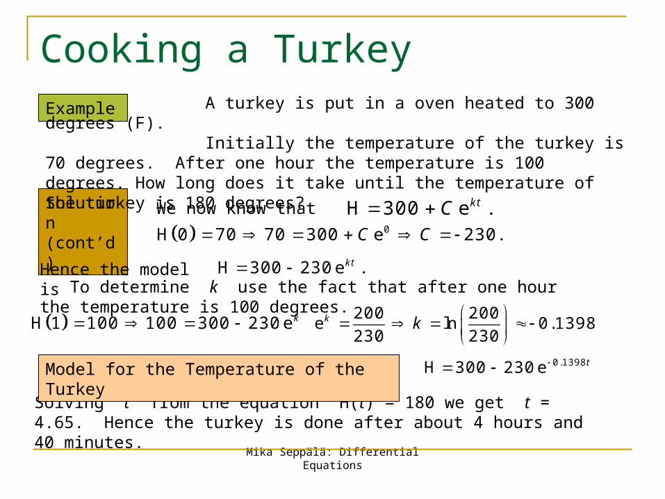
A turkey is put in a oven heated to 300 degrees (F). Initially the temperature of the turkey is 70 degrees. After one hour the temperature is 100 degrees. How long does it take until the temperature of the turkey is 180 degrees?

H 300 e .ktC

Solving t from the equation H(t) = 180 we get t = 4.65. Hence the turkey is done after about 4 hours and 40 minutes.

We now know that

0H 0 70 70 300 e 230.C C

H 1 100 100 300 230ek

H 300 230e .kt Hence the model is

200 200e ln 0.1398

230 230k k

0.1398H 300 230e t Model for the Temperature of the Turkey


Medical ModelingExample

Solution

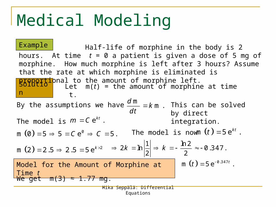
Half-life of morphine in the body is 2 hours. At time t = 0 a patient is given a dose of 5 mg of morphine. How much morphine is left after 3 hours? Assume that the rate at which morphine is eliminated is proportional to the amount of morphine left.

mm.

dk

dt

Let m(t) = the amount of morphine at time t.

2m 2 2.5 2.5 5ek

0m 0 5 5 e 5.C C

e .ktm CThe model is

m 5e .ktt

1 ln22 ln 0.347.

2 2k k

Model for the Amount of Morphine at Time t

By the assumptions we have This can be solved by direct integration.

The model is now

0.347m 5e .tt

We get m(3) ≈ 1.77 mg.

differential equations ordinary differential equations exponential growth or decay families of...

Documents

differential equation

separable equation y

equation gy

substitute y

special solutions y

equation of exponential

type y

constant function y