differential evolution in constrained numerical optimization: an empirical study
TRANSCRIPT

Information Sciences 180 (2010) 4223–4262
Contents lists available at ScienceDirect
Information Sciences
journal homepage: www.elsevier .com/locate / ins
Differential evolution in constrained numerical optimization:An empirical study
Efrén Mezura-Montes a,*, Mariana Edith Miranda-Varela b, Rubí del Carmen Gómez-Ramón c
a Laboratorio Nacional de Informática Avanzada (LANIA A.C.), Rébsamen 80, Centro, Xalapa, Veracruz 91000, Mexicob Universidad del Istmo, Campus Ixtepec, Ciudad Universitaria s/n, Cd. Ixtepec, Oaxaca 70110, Mexicoc Universidad del Carmen, C. 56 #4, Ciudad del Carmen, Campeche 24180, Mexico
a r t i c l e i n f o
Article history:Received 10 October 2009Received in revised form 24 May 2010Accepted 26 July 2010
Keywords:Evolutionary algorithmsDifferential evolutionConstrained numerical optimizationPerformance measures
0020-0255/$ - see front matter � 2010 Elsevier Incdoi:10.1016/j.ins.2010.07.023
* Corresponding author. Tel.: +52 228 841 6100;E-mail addresses: [email protected] (E. M
(R. del Carmen Gómez-Ramón).
a b s t r a c t
Motivated by the recent success of diverse approaches based on differential evolution (DE)to solve constrained numerical optimization problems, in this paper, the performance ofthis novel evolutionary algorithm is evaluated. Three experiments are designed to studythe behavior of different DE variants on a set of benchmark problems by using differentperformance measures proposed in the specialized literature. The first experiment ana-lyzes the behavior of four DE variants in 24 test functions considering dimensionalityand the type of constraints of the problem. The second experiment presents a more in-depth analysis on two DE variants by varying two parameters (the scale factor F and thepopulation size NP), which control the convergence of the algorithm. From the resultsobtained, a simple but competitive combination of two DE variants is proposed and com-pared against state-of-the-art DE-based algorithms for constrained optimization in thethird experiment. The study in this paper shows (1) important information about thebehavior of DE in constrained search spaces and (2) the role of this knowledge in thecorrect combination of variants, based on their capabilities, to generate simple but compet-itive approaches.
� 2010 Elsevier Inc. All rights reserved.
1. Introduction
Nowadays, the use of evolutionary algorithms [12] (EAs) to solve optimization problems is a common practice due totheir competitive performance on complex search spaces [33]. On the other hand, optimization problems usually includeconstraints in their models and EAs, in their original versions, do not consider a mechanism to incorporate feasibility infor-mation in the search process. Therefore, several constraint-handling mechanisms have been proposed in the specializedliterature [6,46].
The most popular approach to deal with the constraints of an optimization problem is the use of (mainly exterior) penaltyfunctions [53], where the aim is to decrease the fitness of infeasible solutions in order to favor the selection of feasible solu-tions. Despite its simplicity, a penalty function requires the definition of penalty factors to determine the severity of thepenalization, and these values depend on the problem being solved [52]. Based on this important disadvantage, several alter-native constraint-handling techniques have been proposed [34].
In the recent years, the research on constraint-handling for numerical optimization problems has been focused mainly inthe following aspects:
. All rights reserved.
fax: +52 228 841 6101.ezura-Montes), [email protected] (M.E. Miranda-Varela), [email protected]

4224 E. Mezura-Montes et al. / Information Sciences 180 (2010) 4223–4262
1. Multiobjective optimization concepts: A comprehensive survey of constraint-handling techniques based on Pareto rank-ing, Pareto dominance, and other multiobjective concepts has been recently published [37]. These ideas have beenrecently coupled with steady-state EAs [64], selection criteria based on the feasibility of solutions found in the currentpopulation [62,63], real-world problems [48], pre-selection schemes [15,31], other meta-heuristics [23], and with swarmintelligence approaches [27].
2. Highly competitive penalty functions: In order to tackle the fine-tuning required by traditional penalty functions, someworks have been dedicated to balance the influence of the value of the objective function and the sum of constraint vio-lation by using rankings [18,52]. Other proposals have been focused on adaptive [1,57,58] and co-evolutionary [17]penalty approaches, as well as alternative penalty functions such as those based on special functions [60,67].
3. Novel bio-inspired approaches: Other nature-inspired algorithms have been used to solve numerical constrained prob-lems, such as artificial immune systems (AIS) [8], particle swarm optimization (PSO) [4,39], and differential evolution(DE) [22,24,38,45,54–57,73–75].
4. Combination of global and local search: Different approaches couple the use of an EA, as a global search algorithm withdifferent local search algorithms. There are combinations such as agent-memetic-based [59], co-evolution-memetic-based [30], and also crossover-memetic-based [61] algorithms. Other approaches combine mathematical-programmingbased local search operators [55,56,65].
5. Hybrid approaches: Unlike the combination of global and local search, these approaches look to combine the advantagesof different EAs, such as PSO and DE [47] or AIS and genetic algorithms (GAs) [2].
6. Special operators: Besides designing operators to preserve the feasibility of solutions [6], there are proposals dedicated toexplore either the boundaries of the feasible and infeasible regions [20,26] or convenient regions close to the parents inthe crossover process [69,71].
7. Self-adaptive mechanisms: There are studies regarding the parameter control in constrained search spaces, such as a pro-posal to control the parameters of the algorithm (DE in this case) [3]. There is another approach where a self-adaptiveparameter control was proposed for the DE parameters and also for the parameters introduced by the constraint-handlingmechanism [42]. The selection of the most adequate DE variant was also controlled by an adaptive approach in [21].Finally, fuzzy-logic has been also applied to control the DE parameters [32].
8. Theoretical studies: Still scarce, there are interesting studies on runtime in constrained search spaces with EAs [72] andalso in the usefulness of infeasible solutions in the search process [68].
Based on this overview of the recent research related with constrained numerical optimization problems (CNOPs), someobservations are summarized:
� The research efforts have been mainly focused on generating competitive constraint-handling techniques (1 and 2 in theprevious list).� The combination of different search algorithms has become very popular (4 and 5 in the list).� Topics related to special operators and parameter control are important to design more robust algorithms to solve CNOPs
(6 and 7 in the aforementioned list).� Besides traditional EAs such as GAs, Evolution Strategies (ES), and Evolutionary Programming (EP), novel nature-inspired
algorithms such as PSO, AIS, and DE have been explored (3 in the list)� DE has specially attracted the interest from researchers due to its excellent performance in constrained continuous search
spaces (last set of references in 3 in the list).
Despite the highly competitive performance showed by DE when solving CNOPs, the research efforts, as it will be pointedout by a careful review of the state-of-the-art later in the paper, have been focused on providing modifications to DE variantsinstead of analyzing the behavior of the algorithm itself. This current work is precisely focused on providing empirical evi-dence about the behavior of DE original variants (without additional mechanisms or modifications) in constrained numericalsearch spaces. Furthermore, this knowledge is used to propose a simple combination of DE variants in a competitive ap-proach to solve CNOPs.
Different experiments are designed to test DE original variants by using, in all cases, an effective but parameter-free con-straint-handling technique. Four performance measures found in the specialized literature are used to analyze the behaviorof four DE variants. These measures are related with the capacity to reach the feasible region, the closeness to the feasibleglobal optimum (or best known solution), and the computational cost. Twenty-four well-known test problems [28] recentlyused to compare state-of-the-art nature-inspired techniques to solve CNOPs are used in the experiments. Nonparametric sta-tistical tests are used to provide more statistical support to the obtained results. It is known from the No Free Lunch Theo-rems for search [66] that using such a limited set of functions does not guarantee, in any way, that a variant which performswell on them, will necessarily be competitive in a different set of problems. However, the main objective of this work is toprovide some insights about the behavior of DE variants depending of the features of the problem. Besides, another goal is toanalyze the effect of two DE parameter values related with its convergence (the scale factor and the population size) on dif-ferent types of constrained numerical search spaces. The last goal of this work is the use of the knowledge obtained in a sim-ple approach which combines the strengths of two DE variants into a single approach which does not use complex additionalmechanisms.
E. Mezura-Montes et al. / Information Sciences 180 (2010) 4223–4262 4225
The paper is organized as follows: In Section 2 the problem of interest is stated. Section 3 introduces the DE algorithm,while in Section 4 a review of the state-of-the-art on DE to solve CNOPs is included. Section 5 presents the analysis proposedin this work. After that, in Section 6 the first experiment on four DE variants in 24 test problems is explained and the ob-tained results are discussed. An analysis of two DE parameters on two competitive (but with different behaviors) DE variantsis presented in Section 7. Section 8 comprises the combination of two DE variants into a single approach and its performanceis compared with respect to some DE-based state-of-the-art approaches. Finally, in Section 9, the findings of the currentwork are summarized and the future paths of research are shown.
2. Statement of the problem
The CNOP, known also as the general nonlinear programming problem [10], without loss of generality can be defined asto:
Find ~x which minimizes
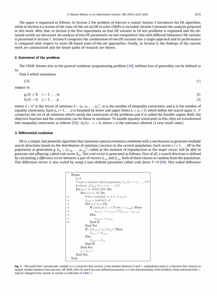
Fig. 1.integermay be
f ð~xÞ ð1Þ
subject to
gið~xÞ 6 0; i ¼ 1; . . . ;m ð2Þhjð~xÞ ¼ 0; j ¼ 1; . . . ;p ð3Þ
where~x 2 Rn is the vector of solutions~x ¼ ½x1; x2; . . . ; xn�T , m is the number of inequality constraints, and p is the number ofequality constraints. Each xi, i = 1, . . . ,n is bounded by lower and upper limits Li 6 xi 6 Ui which define the search space S; Fcomprises the set of all solutions which satisfy the constraints of the problems and it is called the feasible region. Both, theobjective function and the constraints can be linear or nonlinear. To handle equality constraints in EAs, they are transformedinto inequality constraints as follows [52]: jhjð~xÞj � e 6 0, where e is the tolerance allowed (a very small value).
3. Differential evolution
DE is a simple, but powerful algorithm that simulates natural evolution combined with a mechanism to generate multiplesearch directions based on the distribution of solutions (vectors) in the current population. Each vector i, i = 1, . . . ,NP in thepopulation at generation g, ~xi;g ¼ ½x1;i;g ; . . . ; xn;i;g �T , called at the moment of reproduction as the target vector, will be able togenerate one offspring, called trial vector~ui;g . This trial vector is generated as follows: First of all, a search direction is definedby calculating a difference vector between a pair of vectors~xr1 ;g and~xr2 ;g , both of them chosen at random from the population.This difference vector is also scaled by using a user-defined parameter called scale factor F > 0 [50]. This scaled difference
‘‘DE/rand/1/bin” pseudocode. randj[0,1] is a function that returns a real number between 0 and 1. randint[min,max] is a function that returns annumber between min and max. NP, MAX_GEN, CR, and F are user-defined parameters. n is the dimensionality of the problem. Steps indicated with)changed from variant to variant as indicated in Table 1.

4226 E. Mezura-Montes et al. / Information Sciences 180 (2010) 4223–4262
vector is then added to a third vector~xr0 ;g , called base vector. As a result, a new vector is obtained, known as the mutant vector.After that, this mutant vector is recombined, based on a user-defined parameter, called crossover probability 0 6 CR 6 1, withthe target vector (also called parent vector) by using discrete recombination, usually uniform, i.e. binomial crossover, togenerate a trial (child) vector. The CR value determines how similar the trial vector will be with respect to the mutant vector.
Regarding DE variants, in [50], Price et al. present a notation to identify different ways to generate new vectors on DE.The most popular of them (and explained in the previous paragraph) is called DE/rand/1/bin, where the first term means
Fig. 2. DE/rand/1/bin graphical example. ~xi is the target vector, ~xr0 is the base vector chosen at random, ~xr1 and ~xr2 (also chosen at random) are used togenerate the difference vector as to define a search direction. The black square represents the mutant vector, which can be the location of the trial vectorgenerated after performing recombination. The two filled squares represent the other two possible locations for the trial vector after recombination.
Table 1DE variants used in this study. jrand is a random integer number generated between [1,n], where n is thenumber of variables of the problem. randj[0,1] is a real number generated at random between 0 and 1. Bothnumbers are generated using a uniform distribution. ~ui;gþ1 is the trial vector (child vector), ~xr0 ;g is the basevector chosen at random from the current population,~xbest;g is the best vector in the population,~xi;g is the targetvector (parent vector), and ~xr1 ;g and ~xr2 ;g are used to generate the difference vector.
Variant
DE/rand/1/bin:
uj;i;gþ1 ¼xj;r0 ;g þ Fðxj;r1 ;g � xj;r2 ;gÞ if randj½0;1� < CR or j ¼ jrandxj;i;g otherwise
�DE/best/1/bin:
uj;i;gþ1 ¼xj;best;g þ Fðxj;r1 ;g � xj;r2 ;gÞ if randj½0;1� < CR or j ¼ jrandxj;i;g otherwise
�DE/target-to-rand/1:uj;i;gþ1 ¼ xj;i;g þ Fðxj;r0 ;g � xj;i;gÞ þ Fðxj;r1 ;g � xj;r2 ;gÞDE/target-to-best/1:uj;i;gþ1 ¼ xj;i;g þ Fðxj;best;g � xj;i;gÞ þ Fðxj;r1 ;g � xj;r2 ;gÞ
Fig. 3. DE/best/1/bin graphical example. ~xi is the target vector, ~xbest is the base vector (the best vector so far in the population), ~xr1 and ~xr2 (chosen atrandom) are used to generate the difference vector as to define a search direction. The black square represents the mutant vector, which can be the locationof the trial vector generated after performing recombination. The two filled squares represent the other two possible locations for the trial vector afterrecombination.

Fig. 4. DE/target-to-rand/1 graphical example.~xi is the target vector, ~xr0 is the base vector chosen at random, and the difference between them defines afirst search direction.~xr1 and~xr2 (also chosen at random) are used to generate the difference vector as to define a second search direction. The trial vectorwill be located in the black square.
Fig. 5. DE/target-to-best/1/ graphical example. ~xi is the target vector, ~xbest is the base vector (the best vector so far in the population), and the differencebetween them defines a first search direction. ~xr1 and ~xr2 (chosen at random) are used to generate the difference vector as to define a second searchdirection. The trial vector will be located in the black square.
E. Mezura-Montes et al. / Information Sciences 180 (2010) 4223–4262 4227
differential evolution, the second term indicates how the base vector is chosen (at random in this case), the number in thethird term means how many vector differences (i.e. vector pairs) will contribute in the differential mutation (one pair in thiscase). Finally, the fourth term shows the type of crossover utilized (bin from binomial in this variant). The detailed pseudo-code of DE/rand/1/bin is presented in Fig. 1 and a graphical example is explained in Fig. 2.
This study is focused on four DE variants. Two of them are DE/rand/1/bin, explained before, and DE/best/1/bin, where theonly difference with respect to DE/rand/1/bin is that the base vector is not chosen at random; instead, it is the best vector inthe current population. Unlike the first two variants considered in this study, the next two use an arithmetic recombination.They are DE/target-to-rand/1 and DE/target-to-best/1 which only vary in the way the base vector is chosen (at random and thebest vector in the population, respectively). The details of each variant is presented in Table 1 and graphical examples for theremaining three, besides DE/rand/1/bin, are shown in Fig. 3 for the DE/best/1/bin, Fig. 4 for DE/target-to-rand/1 and, finally,Fig. 5 for DE/target-to-best/1.
4. Related work
As it was pointed out in Section 1, DE has provided highly competitive results in constrained numerical search spaces.Therefore, it is a very popular algorithm among researchers and practitioners.
One of the first attempts reported was made by Lampinen [24] with DE/rand/1/bin, where superiority of feasible pointsand dominance in the constraints space were used to bias the search to the feasible global optimum. The approach is knownas Extended DE (EXDE). An extension of Lampinen’s work was presented by Kukkonen and Lampinen [22], where DE/rand/1/bin was then used to solve constrained multiobjective optimization problems with the same constraint-handlingmechanism.
Lin et al. [29] used DE/rand/2/bin with local selection (the target and the base vector are the same) and Lagrange functionsto handle constraints, besides a special mechanisms for diversity control and convergence speed.

4228 E. Mezura-Montes et al. / Information Sciences 180 (2010) 4223–4262
Mezura-Montes et al. [38] used DE/rand/1/bin with three feasibility rules originally proposed by Deb to be used withother EAs [11,49] in an approach called RDE. This algorithm was improved by allowing each target vector to generate morethan one trial vector in [43], called DDE. In a later work, Mezura-Montes et al. [45] proposed a new DE variant where thecombination of the best vector and the target vector is incorporated into the differential mutation operator, coupled witha binomial recombination plus a diversity control, and (again) the chance for each target vector to generate more thanone trial vector. A more recent work by Mezura-Montes and Palomeque-Ortiz [42] included DE/rand/1/bin to explore deter-ministic and self-adaptive parameter control mechanisms in DE for constrained optimization, called A-DDE.
Zielinsky and Laur [73] used DE/rand/1/bin with Deb’s rules [11] coupled with a novel mechanism to deal with boundaryconstraints for decision variable values. They also conducted a study on termination conditions for DE/rand/1/bin in con-strained optimization [74]. These two authors also analyzed the effect of the dynamic tolerance for equality constraintson DE/rand/1/bin [75].
Takahama and Sakai [54] used DE/rand/1/exp with a novel constraint-handling mechanism called � constrained method.They also added a gradient-base mutation to their approach. The authors presented an improved version based on a newcontrol for the � tolerance in [55]. In a recent proposal, they proposed two novel mechanisms to control boundary constraintsto further improve their approach [56].
Tasgetiren and Suganthan [57] proposed a subpopulation mechanism with the combination of DE/rand/1/bin and DE/best/1/bin. Each variant was used with a similar proportion. They opted for an adaptive penalty function to deal with theconstraints.
Huang et al. [21] combined four variants: DE/rand/1/bin, DE/rand/2/bin, DE/target-to-best/2, and DE/target-to-rand/1with a local search mechanism based on Sequential Quadratic Programming. A mechanism to generate random values fortwo DE parameters, CR and F, was included in this proposal and Deb’s rules were used to handle constraints.
Brest [3] proposed jDE-2, which is based on the combined use of DE/rand/1/bin, DE/target-to-best/1/bin, and DE/rand/2/bin. Brest also used Deb’s rules for constraint-handling besides a restart technique for those k worst solutions. In Brest’s ap-proach, each vector had its own parameter values, which were generated and updated with a random-based mechanism.
Landa and Coello [25] used DE/rand/1/bin and Deb’s rules combined with cultural algorithms to incorporate knowledge ofthe problem in the search process.
Huang et al. [19] used DE/rand/1/bin with a co-evolutionary penalty function. One population evolved the penalty factors,while the other evolved the solutions to the optimization problem, similar to the approach proposed with GAs by Coello [5].Huang et al. [20], in their new approach, used DE/rand/1/bin with two sub-populations again, but now with a different goal.The first subpopulation evolved with the aforementioned DE variant, while the second subpopulation stored feasible solu-tions to help other vectors to become feasible. Local search with Nelder–Mead Simplex method was utilized. Instead of usingpenalty functions, Deb’s rules were considered for constraint-handling.
Liu et al. [30] used DE/best/1/bin with a co-evolutionary approach where two sub-populations are considered. One ofthem aimed to minimize the objective function while the other tried to satisfy the constraints of the problem. Gaussianmutation was used as a local search operator and individuals in both sub-populations could migrate from one to another.
Zhang et al. [70] used the stochastic ranking method [52] with DE/rand/1/bin in an approach called Dynamic StochasticSelection DE (DSS-DE) to solve constrained problems.
Gong and Cai [15] used DE/rand/1/bin and Pareto dominance for constraint-handling. They utilized an external file cou-pled with �-dominance to store promising solutions. The initial population was generated with an orthogonal method. A spe-cial operator, orthogonal crossover, was used to improve the local search ability of the algorithm.
Regarding empirical comparisons with DE variants in constrained optimization, Mezura-Montes and López-Ramírez [40]compared DE/rand/1/bin with a global-best PSO, a real-coded GA, and a (l + k)-ES in the solution of 13 benchmark problems.DE provided the best results in this study. Zielinsky et al. [76] compared different adaptive approaches based on DE in con-strained optimization. Other comparisons of DE variants, but in unconstrained optimization, were made by Gämperle et al.[14], where convenient parameter values were found per each test problem, and by Mezura-Montes et al. [44], where thegood performance of each DE variant was linked to an specific type of unconstrained problem.
5. Proposed analysis
From the summary of the state-of-the-art presented in Section 4 it is clear that DE/rand/1/bin is used in more than half ofthe proposed approaches [15,19,20,22,24,25,38,42,70,73–75], while similar variants such as DE/best/1/bin, are barely pre-ferred [30]. The most popular constraint-handling mechanism used with DE is the set of feasibility rules proposed by Deb[3,20–22,24,25,38,42,45,73–75], while penalty functions [19,57] and multiobjective concepts [15,30] are sparingly utilized.There are several approaches which use local search (Gradient-base mutation, Sequential Quadratic Programming, Nelder–Mead Simplex among others) [15,20,21,30,54–56]. On the other hand, there is a tendency to combine different variants inone single approach by adding self-adaptive mechanisms [3] sub-populations [57] or mathematical-programming methods[21]. Finally, the most popular combination is DE/rand/1/bin with Deb’s feasibility rules [20,25,38,42,73–75] or DE/rand/1/bin with a slightly variant of Deb’s rules [22,24].
From the review of the current research in constrained optimization in Section 1, it is clear that DE is a convenient algo-rithm to be modified or combined to solve CNOPs. Furthermore, based on the previous paragraph in this section, it is also

E. Mezura-Montes et al. / Information Sciences 180 (2010) 4223–4262 4229
evident that one variant and one constraint-handling mechanism have been extensively used. However, little knowledgeabout the behavior of DE’s original variants (without additional mechanisms and/or parameters) have been presented, tothe best of the knowledge of the authors, in the specialized literature.
Based on the aforementioned, this work looks precisely to provide more knowledge of the capabilities of DE (by itself) toreach the feasible region of the search space and, even more, the vicinity of the feasible global optimum (or best known solu-tion), the number of evaluations required to do that (i.e. computational cost), and the best combination between computa-tional cost and consistency on generating solutions close to the optimum value.
Furthermore, two DE parameters related with the convergence of the algorithm (the scale factor F and the population sizeNP) are studied in two DE variants with competitive performances, but with different behaviors, in order to (1) detect con-venient values for them, based in the features of the optimization problem and (2) provide some insights on the differencesin the behavior of DE with respect to unconstrained numerical search spaces, reported by Price and Rönkkönen [51].
From the information obtained in the analysis of DE when solving CNOPs, a convenient combination of two DE variants isproposed and its results obtained are compared with respect to those provided by some DE-based algorithms. This proposedapproach does not add complex mechanisms. Instead, it conveniently uses two variants and their strengths into a simpleapproach.
The experimental design utilized in this paper is partially based on a previous study on DE mutations for global uncon-strained optimization proposed in [51]. However some adaptations were made based on the type of problem considered inthis work. In fact, this study only considers the mutation operator in DE variants. Crossover analysis is out of the scope of thepresent research and it is considered as part of the future work.
Three experiments are presented. In the first one, four DE variants are compared. One of them is the most popular in evo-lutionary constrained numerical optimization: DE/rand/1/bin. The second one is barely used: DE/best/1/bin. The third andfourth variants have been used just in combination with other variants to solve CNOPs: DE/target-to-rand/1 and DE/tar-get-to-best/1. The selection of variants was made with the goal to compare popular variants used to solve CNOPs againstthose which use has not been explored. In this way, the findings may help to know the utility of each variant when solvingCNOPs. Nonparametric statistical tests are used to add more confidence to the observed behaviors.
The second experiment analyzes two competitive DE variants, with different behaviors, in order to establish suitablevalues for two DE parameters related with the convergence of the approach (F and NP).
The third experiment tests the combination of two DE variants in different problems and the final results are comparedagainst state-of-the-art approaches.
Different aspects of DE are not considered in this study, such as the number of pairs of difference vectors (one) and, asmentioned before, the crossover effect, i.e. CR = 1. These values remain fixed in both experiments and their studies are con-sidered as part of the future work detailed at the end of the paper.
In order to keep the DE variants from extra-parameters related to the constraint-handling mechanism and also to be con-sistent with the most popular technique reported in the specialized literature, the feasibility criteria proposed by Deb [11]are added as a comparison method (instead of using just the objective function value as indicated in Fig. 1 between the targetand trial vector. The three criteria are the following [11]:
1. If the two vectors are feasible, the one with the best value of the objective function is preferred.2. If one vector is feasible and the other one is infeasible, the feasible one is preferred.3. If the two vectors are infeasible, the one with the lowest normalized sum of constraint violation is preferred.
Four performance measures are utilized during the first two experiments of this work: The first one has been used tomeasure the percentage of runs where feasible solutions are found [28] and the other three were used by Price and Rönkkö-nen [51] to analyze convergence and computational cost. Some terms are defined to facilitate the definition of the perfor-mance measures.
A successful trial is an independent run where the best solution found f ð~xÞ is close to the best known value or optimumsolution f ð~x�Þ. This closeness is measured by a small tolerance on the difference between these two solutions f ð~x�Þ � f ð~xÞ 6 d.A feasible trial is an independent run where, at least, one feasible solution was generated.
The four measures are detailed as follows:
� The feasibility probability FP is the number of feasible trials (f) divided by the total number of tests or independent runsperformed (t), as indicated in Eq. (4).
FP ¼ ft
ð4Þ
The range of values for FP goes from 0 to 1, where 1 means that all independent runs were feasible trials, i.e. all of themreached the feasible region of the search space. In this way, a higher value is preferred.� The probability of convergence P is calculated by the ratio of the number of successful trials (s) to the total number of tests
or independent runs performed (t), as indicated in Eq. (5)
P ¼ st
ð5Þ

4230 E. Mezura-Montes et al. / Information Sciences 180 (2010) 4223–4262
Similar to FP, the range of values for P goes from 0 to 1, where 1 means that all independent runs were successful trials, i.e.all of them converged to the vicinity of the best known solution or the feasible global optimum. Therefore, a higher valueis preferred.� The average number of function evaluations AFES is calculated by averaging the number of evaluations required on each
successful trial to reach the vicinity of the best known value or optimum solution, as indicated in Eq. (6)
AFES ¼ 1s
Xs
i¼1
EVALi ð6Þ
where EVALi is the number of evaluations required to reach the vicinity of the best known value or optimum solution inthe successful trial i. For EVALS, a lower value is preferred because it means that the average cost (measured by the num-ber of evaluations) is lower for an algorithm to reach the vicinity of the feasible optimum solution.� The two previous performance measures (P and AFES) are combined to measure the speed and reliability of a variant
through a successful performance SP, calculated in Eq. (7).
SP ¼ AFESP
ð7Þ
For this measure, a lower value is preferred because it means a better combination between speed and consistency of thealgorithm.
In the next three sections of the paper each experiment is presented. The parameter settings and the test problems usedare detailed, followed by the obtained results and their corresponding discussion.
6. Comparison of DE variants
In this experiment, the four DE variants mentioned in Section 5 and detailed in Section 3 (DE/rand/1/bin, DE/best/1/bin,DE/target-to-rand/1, and DE/target-to-best/1) are compared. A set of 24 benchmark problems used to test nature-inspiredoptimization algorithms in constrained search spaces was used in this experiment. The complete details of all problemscan be found in the Appendix, at the end of the paper, while a summary of their features is presented in Table 2.
The parameters for the four DE variants were the following: CR = 1.0 (this parameter is fixed with this value to discard thecrossover influence from our study), NP = 90, F = 0.9, and MAX_GEN = 5556. The population size value NP for this experimentwas chosen based on two criteria: (1) Enough initial points lead to a generation of more diverse search directions based onvector differences, i.e. a better exploration of the search space and (2) more DE-based approaches to solve CNOPs usepopulation sizes near to this value. The F value was selected based on the suggestions made by Price [50] regarding the
Table 2Details of the 24 test problems [28]. ‘‘n” is the number of decision variables, q = jFj/jSj is the estimated ratio between the feasible region and the search space, LIis the number of linear inequality constraints, NI the number of nonlinear inequality constraints, LE is the number of linear equality constraints, and NE is thenumber of nonlinear equality constraints. a is the number of active constraints at the optimum.
Prob. n Type of function q (%) LI NI LE NE a
g01 13 Quadratic 0.0111 9 0 0 0 6g02 20 Nonlinear 99.9971 0 2 0 0 1g03 10 Polynomial 0.0000 0 0 0 1 1g04 5 Quadratic 52.1230 0 6 0 0 2g05 4 Cubic 0.0000 2 0 0 3 3g06 2 Cubic 0.0066 0 2 0 0 2g07 10 Quadratic 0.0003 3 5 0 0 6g08 2 Nonlinear 0.8560 0 2 0 0 0g09 7 Polynomial 0.5121 0 4 0 0 2g10 8 Linear 0.0010 3 3 0 0 6g11 2 Quadratic 0.0000 0 0 0 1 1g12 3 Quadratic 4.7713 0 1 0 0 0g13 5 Nonlinear 0.0000 0 0 0 3 3g14 10 Nonlinear 0.0000 0 0 3 0 3g15 3 Quadratic 0.0000 0 0 1 1 2g16 5 Nonlinear 0.0204 4 34 0 0 4g17 6 Nonlinear 0.0000 0 0 0 4 4g18 9 Quadratic 0.0000 0 12 0 0 6g19 15 Nonlinear 33.4761 0 5 0 0 0g20 24 Linear 0.0000 0 6 2 12 16g21 7 Linear 0.0000 0 1 0 5 6g22 22 Linear 0.0000 0 1 8 11 19g23 9 Linear 0.0000 0 2 3 1 6g24 2 Linear 79.6556 0 2 0 0 2

Table 3Classification of problems for the first experiment based on the number of decisionvariables.
Class Number of variables Problems
High 10–20 g01, g02, g03, g07, g14, g19, g20, g22Medium 5–9 g04, g09, g10, g13, g16, g17, g18, g21, g23Low 2–4 g05, g06, g08, g11, g12, g15, g24
Table 4Classification of problems for the first experiment based on the type ofconstraints.
Type of constraints Problems
Only inequalities g01, g02, g04, g06, g07, g08, g09,g10, g12, g16, g18, g19, g24
Only equalities g03, g11, g13, g14, g15, g17Inequalities and equalities g05, g20, g21, g22, g23
E. Mezura-Montes et al. / Information Sciences 180 (2010) 4223–4262 4231
convenience of larger F values to avoid premature convergence and also by the corresponding values used in DE-based ap-proaches for CNOPs. The MAX_GEN value was chosen to adjust the maximum number of evaluations of solutions to 500,000,in order to give each DE variant enough time to develop a competitive search, coupled with a high F value and enough searchpoints. The tolerance value for equality constraints was defined as � = 1E�4. The tolerance value for considering a successfultrial was fixed to d = 1E�4. Each variant performed 30 independent runs per each test problem and the four performancemeasures were calculated.
Considering the number of test problems used in this experiment and for a better analysis, they were classified accordingto the dimensionality (number of variables) as indicated in Table 3. Also, they were divided by the type of constraints(inequalities, equalities or both) as shown in Table 4. In this way, the discussion of each performance measure was dividedin three phases: (1) based on the dimensionality of the problem, (2) based on its type of constraints, and finally, (3) somepartial conclusions about the measure results.
6.1. Discussion of results of the first experiment
Problems g20 and g22 were discarded in the discussion because no feasible solutions where found by the four variantscompared (i.e. FP = 0, P = 0, AFES, and SP cannot be calculated). These problems share common features: High-dimensionality(24 and 22 variables, respectively) and combined equality and inequality constraints.
In order to have more confidence of the significant differences observed in the samples, and based on Kolmogorov–Smir-nov tests [9] which indicated that the samples do not follow a Gaussian distribution, nonparametric statistical tests wereapplied to the samples of the AFES measure (Table 7) The Kruskal–Wallis [7] test was applied in test problems where thefour DE variants had samples of equal size, i.e. the same number of successful trials (g04, g06, g08, g12, g16, and g24).The Mann–Whitney test [7] was applied to pairs of variants with different size in the samples (i.e. different number of suc-cessful trials) in the remaining test problems (except g02, g03, g13, and g17, where the results were very poor by the fourvariants compared). Both tests were applied with a significance level of 0.05. The results of the statistical tests indicated thatthe differences observed in the samples are significant, with some exceptions which are commented in Section 6.1.3.
6.1.1. FP measureThe results are presented in Table 5.Dimensionality-based analysis: For high-dimensionality problems, the four DE variants were very competitive. Only
DE/best/1/bin and DE/target-to-rand/1 failed to consistently reach the feasible region in problems g03 and g14. Regardingthe nine medium-dimensionality problems, all four DE variants obtained high FP values. However, they had difficulties togenerate feasible solutions in problems g13 and g23, being DE/target-to-rand/1 the variant with the worst performance.Finally, for low-dimensionality problems, the four variants consistently reached the feasible region, except in problemg05, where DE/target-to-best/1, was the only variant to generate feasible solutions in all independent runs.
Constraint-based analysis: For all the problems with inequality constraints, the four DE variants obtained a goodperformance in the FP measure. However, for all the problems with equality constraints and also in problems g05 andg21 (problems with both type of constraints), only DE/target-to-best/1 consistently reached the feasible region, i.e. DE/rand/1/bin, DE/best/1/bin, and DE/target-to-rand/1 failed in some trials. Furthermore, in problems g13 and g23 this variantprovided the most competitive FP values.
The overall results for the FP performance measure suggest that the four DE variants, without the addition of specialmechanisms or additional parameters, provided a consistent approach to the feasible region, even in presence of a

Table 5FP values obtained by each DE variant on each test problem. Best results are remarked with boldface.
Problem DE/rand/1/bin DE/best/1/bin DE/target-to-rand/1 DE/target-to-best/1
g01 1 1 1 1g02 1 1 1 1g03 1 0.9 0.83 1g04 1 1 1 1g05 0.97 0.93 0.77 1g06 1 1 1 1g07 1 1 1 1g08 1 1 1 1g09 1 1 1 1g10 1 1 1 1g11 1 1 1 1g12 1 1 1 1g13 0.87 0.87 0.3 0.97g14 1 0.93 0.43 1g15 1 1 1 1g16 1 1 1 1g17 1 0.93 0.87 1g18 1 1 1 1g19 1 1 1 1g21 1 0.97 0.97 1g23 0.90 0.90 0.17 0.97g24 1 1 1 1
4232 E. Mezura-Montes et al. / Information Sciences 180 (2010) 4223–4262
combination of inequality and equality constraints. In contrast, as reported in the specialized literature, other EAs usuallyrequire special handling of the tolerance for equality constraints in order to find feasible solutions, [16,36,63]. This is, in fact,a well-documented source of difficulty [35,75]. The most competitive variant in this performance measure was DE/target-to-best/1.
6.1.2. P measureThe results are presented in Table 6.The general behavior, as expected, was different from that observed in the FP measure. It is clear that feasible solutions
found by DE are not necessarily close to the feasible global optimum or best known solution, remarking the difficulty (moreevident for some variants) to move inside the feasible region.
Dimensionality-based analysis: Regarding high-dimensionality problems, the four DE variants presented a very irregularperformance. However, the better average P value for these test problems was provided by DE/target-to-best/1 (0.55),followed by DE/rand/1/bin (0.49), DE/best/1/bin (0.47), and DE/target-to-rand/1 (0.37). The four variants obtained a P = 1
Table 6P values obtained by each DE variant on each test problem. Best results are remarked with boldface.
Problem DE/rand/1/bin DE/best/1/bin DE/target-to-rand/1 DE/target-to-best/1
g01 1 0.8 1 0.87g02 0.03 0 0.13 0g03 0 0.03 0 0g04 1 1 1 1g05 1 1 0.6 0.27g06 1 1 1 1g07 1 0.37 1 1g08 1 1 1 1g09 1 0.93 1 1g10 1 0.2 1 0.67g11 1 0.97 1 1g12 1 1 1 1g13 0 0.27 0 0.03g14 0.93 0.67 0.1 0.43g15 1 1 0.8 0.3g16 1 1 1 1g17 0 0 0.03 0g18 1 0.8 1 0.97g19 0 0.93 0 1g21 0.9 0.5 0.63 0.43g23 0.5 0.5 0 0.43g24 1 1 1 1

E. Mezura-Montes et al. / Information Sciences 180 (2010) 4223–4262 4233
value in medium-dimensionality problems g04 and g16. The average values for the P measure in this type of problems wereas follows: DE/rand/1/bin (0.71), followed by DE/target-to-rand/1 (0.63), DE/target-to-best/1 (0.61), and DE/best/1/bin(0.58). Finally, for low-dimensionality problems DE/rand/1/bin reached a P = 1 value in the seven test problems (average1.0). DE/best/1/bin almost obtained the same value in all problems, except only in problem g11 with P = 0.97 (average0.99). DE/target-to-rand/1 obtained an average value of 0.91 while DE/target-to-best/1 provided an average value of 0.80.
Constraint-based analysis: An almost similar performance (with respect to that observed in the dimensionality-based anal-ysis) was exhibited by the four variants in those problems with only inequality constraints: DE/target-to-best/1/ reached anaverage value of 0.88, DE/target-to-rand/1 (0.86), DE/rand/1/bin (0.85), and DE/best/1/bin (0.77). In problems with onlyequality constraints DE/rand/1/bin and DE/best/1/bin obtained an average P value of 0.49, followed by DE/target-to-rand/1 with 0.32, and DE/target-to-best/1 with 0.29. Finally, in problems with both type of constraints DE/rand/1/bin was clearlysuperior with a P average value of 0.80. DE/best/1/bin obtained a value of 0.67, DE/target-to-rand/1 0.41, and DE/target-to-best/1 0.38.
Despite the fact that the four DE variants were very capable to reach the feasible region of the search space (based on theresults of the FP measure explained before), the results for the P measure indicate that they presented difficulties to reach the
Table 7AFES values obtained by each DE variant on each test problem. Best results are remarked with boldface. ‘‘–” means that the performance measure was notdefined for this problem/variant.
Problem DE/rand/1/bin DE/best/1/bin DE/target-to-rand/1 DE/target-to-best/1
g01 361679.33 37135.17 311840.07 33770.04g02 401419.00 – 472004.25 –g03 – 104859.00 – –g04 41756.13 22949.40 40342.37 21687.03g05 233141.67 88544.47 340144.89 64530.75g06 16902.00 11886.30 16677.87 18429.37g07 298298.50 59669.55 237150.83 59828.50g08 2597.90 1732.83 2553.07 1832.67g09 77154.70 28459.21 62958.03 27866.17g10 205181.10 75590.50 170220.43 51686.05g11 22051.90 9649.76 76508.90 31771.77g12 7976.63 3903.03 11003.67 7330.00g13 – 169700.63 – 316734.00g14 229520.11 70108.05 233873.33 95154.08g15 101919.40 69464.63 221034.54 184372.00g16 36011.43 16112.70 32605.73 15506.43g17 – – 266434.00 –g18 221071.67 53699.04 229835.00 42043.41g19 – 122569.11 – 86005.70g21 105550.63 44098.13 143494.00 47643.38g23 416715.00 170003.73 – 182492.77g24 7165.30 4780.37 6994.37 4669.67
Fig. 6. Radial graphic for those test problems where the AFES values were less than 80,000 for all variants.

Table 8SP values obtained by each DE variant on each test problem. Best results are remarked with boldface.‘‘–” means that the performance measure was not definedfor this problem/variant.
Problem DE/rand/1/bin DE/best/1/bin DE/target-to-rand/1 DE/target-to-best/1
g01 3.62E+05 4.64E+04 3.12E+05 3.90E+04g02 1.20E+07 – 3.54E+06 –g03 – 3.15E+06 – –g04 4.18E+04 2.29E+04 4.03E+04 2.17E+04g05 2.33E+05 8.85E+04 5.67E+05 2.42E+05g06 1.69E+04 1.19E+04 1.67E+04 1.84E+04g07 2.98E+05 1.63E+05 2.37E+05 5.98E+04g08 2.60E+03 1.73E+03 2.55E+03 1.83E+03g09 7.72E+04 3.05E+04 6.30E+04 2.79E+04g10 2.05E+05 3.78E+05 1.70E+05 7.75E+04g11 2.21E+04 9.98E+03 7.65E+04 3.18E+04g12 7.98E+03 3.90E+03 1.10E+04 7.33E+03g13 – 6.36E+05 – 9.50E+06g14 2.46E+05 1.05E+05 2.34E+06 2.20E+05g15 1.02E+05 6.95E+04 2.76E+05 6.15E+05g16 3.60E+04 1.61E+04 3.26E+04 1.55E+04g17 – – 7.99E+06 –g18 2.21E+05 6.71E+04 2.30E+05 4.35E+04g19 – 1.31E+05 – 8.60E+04g21 1.17E+05 8.82E+04 2.27E+05 1.10E+05g23 8.33E+05 3.40E+05 – 4.21E+05g24 7.17E+03 4.78E+03 6.99E+03 4.67E+03
Fig. 7. Radial graphic for those test problems where the SP values were less than 80,000 for all variants.
4234 E. Mezura-Montes et al. / Information Sciences 180 (2010) 4223–4262
vicinity of the feasible global optimum or best known solution. DE/rand/1/bin provided the most consistent approach to thebest feasible solution (average P value of 0.74), followed by DE/best/1/bin (average P value 0.68). Finally, DE/target-to-best/1was competitive in high-dimensionality problems and in presence of only inequality constraints.
6.1.3. AFES measureThe results are presented in Table 7.Dimensionality-based analysis: DE/best/1/bin was the most competitive variant in high-dimensionality problems with an
average AFES value of 7.89E+04 in five test problems (out of six), followed by DE/target-to-best/1 with 6.87E+04 but only infour test problems. From the statistical test results, the performance of these two best-based variants was not significantlydifferent in problems g07 and g19. The two rand-based variants were less competitive: DE/target-to-rand/1 with 3.14E+05and DE/rand/1/bin with 3.23E+05, both in four test problems. A similar behavior was found in medium-dimensionality prob-lems. DE/best/1/bin was the best variant with an average value of 7.26E+04 in eight problems (out of nine), followed by DE/target-to-best/1 with 8.82E+04 in eight problems, (no significant differences were found by these two best-based variants in

E. Mezura-Montes et al. / Information Sciences 180 (2010) 4223–4262 4235
problems g09, g10, g21, and g23). DE/target-to-rand/1 obtained an average value of 1.35E+05 and DE/rand/1/bin presented avalue of 1.58E+05, both in seven test problems. In low-dimensionality problems the results were quite similar as well: DE/best/1/bin was the best variant with an average value of 2.71E+04 in the seven test problems, DE/target-to-best/1 obtained avalue of 4.47E+04 in the seven problems (no significant differences were found in problems g05 and g15), DE/rand/1/bin andDE/target-to-rand/1 achieved average values of 5.60E+04 and 9.64E+04, respectively, in the seven test problems.
Constraint-based analysis: In problems with only inequality constraints the four variants succeeded in 12 out of 13 testproblems. However, DE/target-to-best/1 was the most competitive with an AFES average value of 3.09E+04, DE/best/1/binwas the second best with a value of 3.65E+04 (from the statistical tests no significant differences were found in problemsg07, g09, g10, and g19). The two rand-based variants were less competitive: DE/target-to-rand/1 with 1.33E+05 and DE/rand/1/bin with 1.40E+05. The presence of only equality constraints did not prevent DE/best/1/bin to be the most compet-itive with an average AFES value of 8.48E+04 on five (out of six) test problems. The second best performance was obtained byDE/target-to-best/1 with 1.57E+05 in four test problems (no significant differences were observed in problem g15). DE/tar-get-to-rand obtained an average value of 1.99E+05 in four problems. DE/rand/1/bin reached a value of 1.18E+05 but in only
Table 9(a) Test problems with a different dimensionality.(b) Test problems with different type of constraints.
Problem Dimensionality
(a)g02 Highg21 Mediumg06 Low
Problem Type of constraints
(b)g10 Inequalitiesg13 Equalitiesg23 Both of them
Fig. 8. Results obtained in the three performance measures by DE/rand/1/bin in problem g02.

4236 E. Mezura-Montes et al. / Information Sciences 180 (2010) 4223–4262
three test problems. Finally, in problems with both type of constraints, DE/target-to-best/1 was the most competitive withan average value of 9.82E+04 in the three test problems, followed by DE/best/1/bin with a value of 1.01E+05 also in the threetest problems (no significant differences were exhibited in problems g05, g21, and g23). DE/rand/1/bin obtained a value of2.52E+05 in three test problems while DE/target-to-rand/1 reached an average value of 2.42E+05 but in only two problems.
The overall results regarding AFES suggest that those best-based variants found the vicinity of the best known or optimalsolution faster than the rand-based variants. DE/best/1/bin was the most competitive variant.
Fig. 6 shows a radial graphic where the AFES values are shown and each axis is associated with one DE variant. For a bettervisualization only those test problems with a value below 80,000 for the AFES measure are presented, but the overall behav-ior is represented. A point near the origin is better, because it represents a lower AFES value. It is remarked in this figure thatboth best-based variants required less evaluations with respect to the two rand-based variants.
6.1.4. SP measureThe results are presented in Table 8.Dimensionality-based analysis: In a similar way with respect to the AFES measure, the best-based variants performed bet-
ter in the SP measure in this classification of problems. For high-dimensionality problems DE/best/1/bin obtained a SP aver-age value of 7.18E+05 on five (out of six) test problems, DE/target-to-best/1 reached a value of 1.01E+05 on four problems,followed by DE/target-to-rand/1 with 1.61E+06 on four problems, and DE/rand/1/bin with 3.24E+06 also in four problems.DE/best/1/bin obtained the best SP average value in medium-dimensionality problems with 1.97E+05 on eight (out of nine)test problems, DE/target-to-best/1 was second with 1.28E+06 also on eight problems, DE/rand/1/bin was third with 2.19E+05in only seven problems, and DE/target-to-rand/1 was fourth with 1.25E+06 in seven test problems. In low-dimensionalityproblems DE/best/1/bin presented the lowest SP average value on the seven test problems (2.72E+04). DE/rand/1/bin wassecond with 5.60E+04 also in the seven problems. DE/target-to-best/1 was third with 1.32E+05 in the seven problems.DE/target-to-rand/1 was the last with an average SP of 1.37E+05 also in the seven test problems.
Constraint-based analysis: DE/target-to-best/1 showed the lowest SP average (3.36E+04) for the test problems with onlyinequality constraints (12 out of 13), followed by DE/best/1/bin with 7.31E+04 in 12 problems, DE/target-to-rand/1 with3.89E+05 and DE/rand/1/bin with 1.11E+06, both computed in 12 problems. The best SP average value in five (out of six)problems with only equality constraints was obtained by DE/best/1/bin with 7.93E+05, followed by DE/target-to-best/1 with2.59E+06 in four test problems, DE/target-to-rand/1 with 2.67E+06 in four test problems. The worst SP values were obtainedby DE/rand/1/bin with 1.23E+05 but in only three test problems. Finally, in problems with equality and inequality
Fig. 9. Results obtained in the three performance measures by DE/best/1/bin in problem g02.
E. Mezura-Montes et al. / Information Sciences 180 (2010) 4223–4262 4237
constraints DE/best/1/bin dominated the remaining DE variants with an average SP value (in the three test problems) of1.72E+05, followed by DE/target-to-best/1 with 2.58E+05 also in the three problems. DE/rand/1/bin was third with3.95E+05 in the three problems, while DE/target-to-rand/1 was fourth with 3.97E+05, but computed in only two testproblems.
The overall performance presented in the SP measure resembles that found in the AFES measure. The best-based DEvariants outperformed those rand-based. This is also noted in Fig. 7, where the lowest SP values, i.e. the best combinationbetween computational cost (evaluations) and successful trials (reaching the vicinity of the feasible best known or optimumsolution) were found by the two best-based DE variants. In fact, DE/best/1/bin was, again, the most competitive variant onthis measure. As in Fig. 6, for a better visualization, Fig. 7 only included values below 80,000 for the SP measure, but the over-all behavior is represented.
6.2. Conclusions of the first experiment
Interesting findings were obtained from this first set of experiments:
� Regardless of the DE variant used, DE itself showed strong capabilities to reach the feasible region of the search space inthe benchmark problems utilized in this work. The dimensionality of the problems and the type of constraints did notaffect this convenient behavior. DE/target-to-best/1 was the most consistent DE variant on this regard.� DE/rand/1/bin showed the best performance regarding the percentage of successful trials (runs where the vicinity of the
feasible global optimum or best known solution was reached) followed by DE/target-to-rand/1.� Those best-based variants, mostly DE/best/1/bin, required significant less evaluations to reach the vicinity of the feasible
global optimum or best known solution.� DE/best/1/bin obtained the best combination between computational cost (measured by the number of evaluations to
reach the best solution in the search space) and the percentage of successful trials.� DE/target-to-best/1 and DE/target-to-rand/1 did not provide a significant better performance with respect to DE/rand/1/
bin and DE/best/1/bin. However, DE/target-to-best/1 was very competitive in high-dimensionality problems and in thosetest functions where only inequality constraints were considered. Finally, based on the statistical tests performed, thisvariant was equally competitive, regarding the AFES measure values, with respect to DE/best/1/bin in eight test problems.
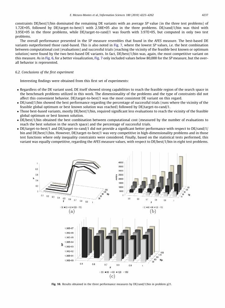
Fig. 10. Results obtained in the three performance measures by DE/rand/1/bin in problem g21.

4238 E. Mezura-Montes et al. / Information Sciences 180 (2010) 4223–4262
Additional results were obtained with the same structure of this experiment but varying the NP value and keeping thesame limit of evaluations (500,000). The values for the population size were NP = 30 and NP = 150. The results are includedin [41] and confirmed the findings previously commented.
Those findings motivated a more in-depth analysis of the two most competitive variants: DE/rand/1/bin, being the mostconsistent on reaching the vicinity of the feasible optimum solution, and DE/best/1/bin, with the best combination betweenthe number of evaluations required and the number of successful trials. The corresponding experiments and results aredescribed in the next section.
7. DE parameter study
The second set of experiments aims to determine the convenient values and the relationship between two DE parametersin the performance of two DE variants which exhibited different competitive behaviors in numerical constrained searchspaces, based on the findings of the first set of experiments (DE/rand/1/bin and DE/best/1/bin).
The parameters considered are F and NP. As the stepsize in differential mutation is controlled by F, the convergence speeddepends of its value. Regarding global unconstrained optimization, for low F values (to speed up convergence) an increase inthe NP value may be required to avoid premature convergence [51]. The question remains open for numerical spaces in pres-ence of constraints. It is known in advance, from the set of experiments in Section 6, that DE/rand/1/bin is more consistent onreaching the vicinity of the feasible best solution and that DE/best/1/bin is also capable to do it but with a lower frequencycombined with an also lower computational cost. The experimental design now focuses on determining the best values forthose two aforementioned parameters for these variants and evaluating if the behavior is similar to that found in uncon-strained search spaces.
Six representative test problems are used in this second part of the research: g02, g06, g10, g13, g21, and g23. They wereselected based on their different characteristics and were organized as follows:
� Test problems with different dimensionality. They are shown in Table 9a).� Test problems with different type of constraints. They are presented in Table 9b).
Fig. 11. Results obtained in the three performance measures by DE/best/1/bin in problem g21.

E. Mezura-Montes et al. / Information Sciences 180 (2010) 4223–4262 4239
The parameter values for the two DE variants were the following: CR = 1.0, the Gmax was not considered because the ter-mination condition was, in all cases, 500,000 evaluations computed, the tolerance value for equality constraints was� = 1E�4, and the tolerance value to consider as successful an independent run was d = 1E�4; the F values were the follow-ing: [0.1,0.2,0.3,0.4,0.5,0.6,0.7,0.8,0.9,1.0] and those of NP were: [30,60,90,120,150]. Each DE variant was executed 100times per each test problem per each combination of F and NP values. Three performance measures (P, AFES, and SP) wereused in the following experiments. The FP measure was not considered because both DE variants are able to reach the fea-sible region consistently (based on the results obtained in the first set of experiments). The results are presented as follows:One graph is presented for each performance measure. In each graph, the horizontal axis includes the different F values,while the corresponding value for the measure is indicated in the vertical axis. The inclined axis includes the five NP values.There is one line or set of bars for each NP value previously defined. Some graphs for the AFES and SP measures do not con-sider either some F or NP values because the measure value was not defined for such parameter value. For a better visual-ization, the SP values are plotted with a nonlinear scale.
7.1. High-dimensionality test problem
Figs. 8 and 9 exhibit the graphs with the results obtained by DE/rand/1/bin and DE/best/1/bin, respectively, for problemg02.
A quick look in Figs. 8 and 9 clearly reveals that both variants were very sensitive to the two parameter values analyzedand that the results obtained were poor.
In Fig. 8(a) DE/rand/1/bin provided some successful trials (P 6 0.6) only with 0.5 6 F 6 0.9 combined with medium tolarge population 90 6 NP 6 150. The highest P value was obtained with F = 0.7 and NP = 120.
The results in Fig. 8(b) suggest that for DE/rand/1/bin, as the scale factor value increased, the average number of evalu-ations also increased for the three NP values where successful trials were found (90, 120, and 150). Larger populations(NP = 150) performed less evaluations with lower F values (F = 0.5), while smaller populations required higher F values(F = 0.7).
Fig. 8(c) presents the SP values obtained by DE/rand/1/bin. It is clear that the best combination of convergence speed(AFES) and probability of convergence (P) was obtained by this variant in medium to larger populations (90 6 NP 6 150) with0.6 6 F 6 0.7.
Fig. 12. Results obtained in the three performance measures by DE/rand/1/bin in problem g06.
4240 E. Mezura-Montes et al. / Information Sciences 180 (2010) 4223–4262
DE/best/1/bin, as shown in Fig. 9(a) could not reach the vicinity of the best known solution except in one single run withF = 0.8 and NP = 150 (see also Fig. 9(b) and (c)).
DE/rand/1/bin was clearly most competitive in this large search space, where the challenge is to find the best known solu-tion because almost all solutions are feasible. This behavior suggests that larger populations (120 6 NP 6 150), combinedwith 0.6 6 F 6 0.7 increase the probability of this variant to reach the vicinity of the best known solution with a moderatedcomputational cost measured by the number of evaluations utilized.
7.2. Medium-dimensionality test problem
The values obtained by each DE variant in the three performance measures when solving problem g21 are summarized inFigs. 10 and 11.
Regarding the P measure, DE/rand/1/bin presented a similar behavior to that showed by DE in unconstrained optimiza-tion [51], because the convergence to the feasible global optimum was obtained when high F and NP values were utilized. Itwas also obtained by the combination of low scale factor values (0.5 6 F 6 0.6) but with larger population sizes(60 6 NP 6 150) (see Fig. 10(a)). Regarding high F values (except F = 1.0), this variant displayed also high P values for allpopulation sizes.
Regarding the average of number of evaluations required by DE/rand/1/bin, Fig. 10(b) exhibits an increment of the AFESvalue as the scale factor and population size values increased their values as well, i.e. this variant did not require largerpopulations nor high F values to provide a competitive performance.
Fig. 10(c) confirms the behavior observed in the results of the AFES measure, because the best mix of computational costand convergence was obtained by small populations (30 6 NP 6 60) combined with the following scale factor values(0.6 6 F 6 0.8).
DE/best/1/bin presented a similar behavior with respect to DE/rand/1/bin in the P measure. However, the following highscale factor values 0.7 6 F 6 1.0 provided high P values combined with medium-large population sizes (90 6 NP 6 150), seeFig. 11(a).
The results for the AFES measure in Fig. 11(b) present the lowest values with NP = 30. However the P values for thispopulation size (Fig. 11(a)) were very poor. Therefore, the better AFES values were obtained by DE/best/1/bin with mediumsize populations (60 6 NP 6 90) combined with F = 0.7. It is worth noticing that medium size populations presented thehighest AFES values in combination with the highest F value used (1.0).
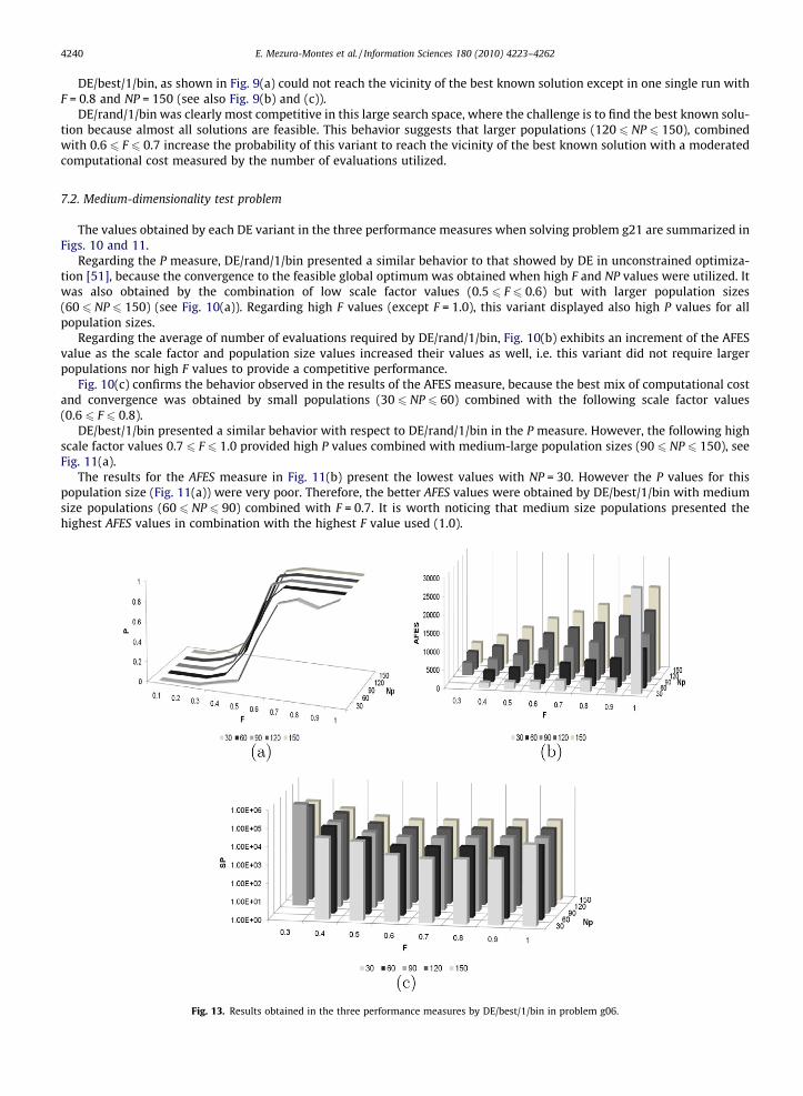
Fig. 13. Results obtained in the three performance measures by DE/best/1/bin in problem g06.

E. Mezura-Montes et al. / Information Sciences 180 (2010) 4223–4262 4241
The SP values in Fig. 11(c) reveal that the best compound effect speed-convergence were provided by small-medium sizepopulations (60 6 NP 6 90) with F = 0.8.
Both DE variants were competitive in this problem with medium dimensionality. However, DE/rand/1/bin was less sen-sitive to the two parameters under study, by working well with small and medium population sizes combined with threedifferent scale factor values. Similarly, DE/best/1/bin was more competitive with small and medium size populations butwith just one scale factor value.
7.3. Low-dimensionality test problem
Figs. 12 and 13 present the results for the three measures obtained by both compared variants in test problem g06.DE/rand/1/bin obtained some feasible trials with low scale factor values 0.4 6 F 6 0.5 combined with larger population
sizes (120 6 NP 6 150) in Fig. 12(a). Values of P = 1.0 were consistently obtained with 0.6 6 F 6 1.0 combined with the fourNP values (except NP = 30).
Fig. 12(b) includes the results for the AFES measure. The observed behavior indicates an increment in the value of themeasure as the population size and the scale factor values are also increased.
Most of the combination NP–F values provided low SP values, as indicated in Fig. 12(c) (only low F values with largerpopulations obtained poor SP values). However, a small population (NP = 30) combined with 0.6 6 F 6 1.0 are the mostconvenient values to solve this problem.
DE/best/1/bin required slightly higher scale factor values (0.7 6 F 6 1.0) to consistently reach the vicinity of the globaloptimum (P = 1.0), except with NP = 30 (see Fig. 13(a)).
A similar effect was obtained by DE/best/1/bin in the AFES measure with respect to DE/rand/1/bin (higher F and larger NPvalues caused higher AFES values). However, with NP = 30 and F = 1.0 the highest AFES value was obtained (see Fig. 13(b)).
The summary of results for the SP measure in Fig. 13(c) indicates that a small population NP = 30 combined with0.7 6 F 6 0.8 provided the best blend between number of evaluations and convergence probability.
Both DE variants presented an almost similar behavior in this problem with only two decision variables, i.e. they requireda small population to provide a consistent approach to the vicinity of the feasible global optimum. However, DE/best/1/binwas slightly more sensitive to the F parameter.
Fig. 14. Results obtained in the three performance measures by DE/rand/1/bin in problem g10.

4242 E. Mezura-Montes et al. / Information Sciences 180 (2010) 4223–4262
7.4. Test problem with only inequality constraints
Figs. 14 and 15 include the results provided by both variants when solving problem g10.DE/rand/1/bin provided high P values with more consistency by using medium size populations (60 6 NP 6 90) combined
with high scale factor values (0.6 6 F 6 1.0) in Fig. 14(a). Increasing the population size (NP = 150) with lower scale factorvalues (F = 0.5) allowed DE/rand/1/bin to maintain high P values.
The results for the AFES measure in Fig. 14(b) confirms the convenience of using medium size populations, mostly with0.6 6 F 6 0.7. Other combination of values for these two parameters increased the AFES value (with the only exception ofNP = 30 and F = 0.8).
Fig. 14(c) also confirms the findings previously discussed for DE/rand/1/bin in this test problem. The lowest SP valueswere found with NP = 60 and F = 0.6.
In Fig. 15(a) DE/best/1/bin required larger populations to get successful trials more consistently (120 6 NP 6 150) com-bined with high scale factor values (0.8 6 F 6 0.9). DE/best/1/bin was clearly affected by small populations, regardless thescale factor value used.
The overall results for the AFES measure in Fig. 15(b) suggest that DE/best/1/bin increased the number of evaluations as Fand NP values also increased. Furthermore, the lowest AFES values were obtained with medium size populations(60 6 NP 6 90). However, the P values for this population size were poor.
This last finding was confirmed in Fig. 15(c), where the lowest SP values were obtained with medium to larger popula-tions (90 6 NP 6 150) combined with 0.7 6 F 6 0.9.
DE/rand/1/bin was less sensitive to both parameters analyzed and performed better with small-medium size populations.However, DE/best/1/bin required less evaluations to provide competitive results by using larger populations.
7.5. Test problem with only equality constraints
Figs. 16 and 17 present the summary of results in problem g13 by DE/rand/1/bin and DE/best/1/bin, respectively.Similar to the problem with a high-dimensionality, the performance of both variants was clearly affected in this test
function.
Fig. 15. Results obtained in the three performance measures by DE/best/1/bin in problem g10.

E. Mezura-Montes et al. / Information Sciences 180 (2010) 4223–4262 4243
DE/rand/1/bin was able to provide its best P values (below 0.5) with only high scale factor values (0.6 6 F 6 1.0) combinedwith small and medium population sizes (30 6 NP 6 90). However, the most consistent results for P were obtained withNP = 60 (see Fig. 16(a)).
The lowest AFES values were found with NP = 30 and 0.7 6 F 6 1.0 (see Fig. 16(b)). It is interesting to note that largerpopulations (NP = 120) combined with 0.6 6 F 6 0.7 presented the highest AFES values.
The best composite of convergence speed and convergence probability (SP value) was obtained with NP = 30 combinedwith F = 0.7 and F = 1.0, and also with NP = 60 combined with F = 0.7 (see Fig. 16(c)).
Based on Fig. 17(a), DE/best/1/bin provided more successful trials with high scale factor values (0.7 6 F 6 1.0) combinedwith larger populations (120 6 NP 6 150). Moreover, with medium size populations (60 6 NP 6 90) required higher scalefactor values (0.8 6 F 6 1.0). Unlike DE/rand/1/bin, this variant had significant difficulties to reach the vicinity of the bestknown solution with a small population.
Fig. 17(b) indicates that the lowest AFES values were obtained with NP = 30 combined with 0.9 6 F 6 1.0, followed byNP = 60 combined with 0.8 6 F 6 1.0. The highest AFES values were obtained with the highest NP and F values as well.
The results for the SP measure in Fig. 17(c) pointed out that the best combination of AFES and P values were obtained withNP = 60 and 0.8 6 F 6 1.0.
Both DE variants had difficulties to reach the vicinity of the feasible global optimum. Interestingly, both variants per-formed better with medium size populations with very similar scale factor values. However, DE/rand/1/bin required slightlylower F values and obtained better results with a small population with respect to DE/best/1/bin.
7.6. Test problem with both type of constraints
The results obtained by both variants in problem g23 are presented in Figs. 18 and 19 for DE/rand/1/bin and DE/best/1/bin, respectively.
Based on Fig. 18(a), competitive P values were consistently achieved by DE/rand/1/bin with NP = 60 combined with0.6 6 F 6 1.0. A very irregular behavior was observed with large and small populations. The results for the P measure werevery poor with F = 1.0 (except with NP = 60).
The lowest average number of evaluations on successful trials were attained by DE/rand/1/bin with small to mediumpopulation sizes (30 6 NP 6 60) combined with 0.8 6 F 6 0.9 and 0.6 6 F 6 0.7, respectively (see Fig. 18(b)). Largerpopulations (NP = 150) caused an increment in the AFES value.
Fig. 16. Results obtained in the three performance measures by DE/rand/1/bin in problem g13.

Fig. 17. Results obtained in the three performance measures by DE/best/1/bin in problem g13.
4244 E. Mezura-Montes et al. / Information Sciences 180 (2010) 4223–4262
The best SP values were obtained in the same combination of parameter values observed for the AFES measure (seeFig. 18(c)).
In contrast to DE/rand/1/bin, DE/best/1/bin, in Fig. 19(a), obtained more successful trials with larger populations NP = 150combined with high scale factor values (0.7 6 F 6 1.0). The vicinity of the feasible best known solution was not reached witha small population (NP = 30).
The lowest AFES values were obtained by DE/best/1/bin with NP = 90 in all the F values where P > 0 values were obtained(0.7 6 F 6 1.0), see Fig. 19(b).
Regarding the SP values (Fig. 19(c)), the best values were found with NP = 90 combined with 0.8 6 F 6 0.9.In this last test problem, DE/rand/1/bin performed better with small to medium size populations combined with different
scale factor values. In contrast, DE/best/1/bin provided its best performance with medium to larger populations coupled onlywith high scale factor values.
7.7. Conclusions of the second experiment
The findings of this second experiment are summarized in the following list:
� DE/rand/1/bin was clearly most competitive in the high-dimensionality test problem.� DE/rand/1/bin was the variant with less sensitivity to NP and F in all the six test problems.� DE/best/1/bin required less evaluations to reach the global feasible optimum in all the test problems, but it was less reli-
able than DE/rand/1/bin.� The most useful F values for both variants were 0.6 6 F 6 0.9, regardless the type of test problem.� DE/rand/1/bin/ performed better with small to medium size populations: 30 6 NP 6 90, while DE/best/1/bin required
more vectors in its population to provide competitive results 90 6 NP 6 150.� Regarding the convergence behavior reported in unconstrained numerical optimization with DE, a different comportment
was observed in the constrained case, because low scale factor values (F 6 0.5) prevented both DE variants to converge,even with larger populations. The exception was the test problem with a low-dimensionality.

Fig. 18. Results obtained in the three performance measures by DE/rand/1/bin in problem g23.
E. Mezura-Montes et al. / Information Sciences 180 (2010) 4223–4262 4245
Additional experiments were performed in test problems with similar features as those presented in the paper: g19 forhigh-dimensionality, g09 for medium-dimensionality, g08 for low-dimensionality, g07 with only inequality constraints, g17with only equality constraints, and g05 with both type of constraints. Those results can be found in [41] and they confirmedthe findings mentioned above.
The summary of findings suggests that the ability of DE/rand/1/bin to generate search directions from different base vec-tors allows it to use smaller populations. On the other hand, larger populations were required by DE/best/1/bin, where thesearch directions are always based on the best solution so far. Regarding the scale factor, the convenient values found in theexperiment showed that these two DE variants required a slow-convergence behavior to approach the vicinity of the feasibleglobal optimum or best known solution. To speed up the convergence by decreasing the scale factor value does not seem tobe an option, even with larger populations. The combination of larger populations and DE/rand/1/bin seems to be more suit-able for high-dimensionality problems. Finally, DE/rand/1/bin presented less sensitivity to the two parameters analyzed.Meanwhile, DE/best/1/bin, which may require a more careful fine-tuning, can provide competitive results with a lower num-ber of evaluations. Based on this last comment, the drawback found in DE/best/1/bin may be treated with parameter controltechniques [13].
8. A combination of two DE variants
Considering the results in Experiment 1 which pointed out that DE/rand/1/bin and DE/best/1/bin had better performancesbut different behaviors with respect to other DE variants, they were chosen to be combined into one single approach.
The capacity observed in the four DE variants to efficiently reach the feasible region of the search space in Experiment 1,coupled with the feature of DE/rand/1/bin to generate a more diverse set of search directions, suggested the use of thisvariant as a first search algorithm. As the feasible region will be reached faster, the criterion to switch to the other DE variantwas to get 10% of feasible vectors. In this way, DE/best/1/bin could focus the search in the vicinity of the current best feasiblevector, expecting a low number of evaluations to reach competitive solutions. This percentage value was chosen after sometests reported in [41]. The approach was called Differential Evolution Combined Variants (DECV).
Based on the fact that Experiment 2 revealed that DE/rand/1/bin performed better with small to medium size populationsand that DE/best/1/bin required medium to large size populations, the number of vectors in DECV was fixed to 90. The

Fig. 19. Results obtained in the three performance measures by DE/best/1/bin in problem g23.
4246 E. Mezura-Montes et al. / Information Sciences 180 (2010) 4223–4262
convenience of using larger F values also observed in Experiment 2 suggested a value of 0.9. The CR parameter was kept fixedat 1.0 and the number of generations was set to 2666 in order to perform 240,000 evaluations.
Thirty independent runs per each one of the 24 test problems used in Experiment 1 were computed. Statistics on the finalresults are summarized in Tables 10 and 11 for DECV.
Those final results for the first 13 test problems and the corresponding computational cost, measured by the number ofevaluations required, were compared with those reported by some state-of-the-art DE-based algorithms: The superiority offeasible points (EXDE) [24], the feasibility rules [11] in DE (RDE) [38], the DE with ability to generate more than one trialvector per target vector [43] (DDE), the adaptive DE (A-DDE) [42], and the dynamic stochastic selection in DE (DSS-MDE)[70]. The comparison in the last 11 test problems was made with respect to A-DDE in Table 11, which has provided a highlycompetitive performance in such problems. Both, EXDE [24] and RDE [38] were chosen because of the fact that they keepintact the DE mutation operator with respect to its original version. DDE [43] was chosen as a DE with modifications tothe original mutation operator with very competitive results and, finally, DSS-MDE [70] was chosen as a recent representa-tive approach. The results of the approaches used for comparison were taken from [70].
DECV reached the feasible region of the search space in every single run for 22 test problems (except in problems g20 andg22). Regarding the first 13 problems, DECV was able to consistently reach the best known solution in seven test problems(g04, g05, g06, g08, g09, g11, and g12). Moreover, DECV found the best known solution in some runs in three test problems(g01, g07, and g10), but was unable to provide good results in three test problems (g02, g03, and g13). The overall behaviorshowed a very competitive performance with respect to the compared algorithms. The number of evaluations required byDECV was 240,000, higher than the 180,000 required by A-DDE [42], the 225,000 required by DSS-MDE [70] and DDE[43], and lower than the 350,000 computed by RDE [38]. It is important to remark that A-DDE utilizes a self-adaptive mecha-nism similar to that used in Evolution Strategies [42], which adds extra computational time to the algorithm, DDE requiresthe careful fine-tuning of extra-parameters related with the number of trial vectors generated per each target vector andanother parameter to control diversity in the population, and DSS-MDE utilizes a dynamic mechanism to deal with the sto-chastic ranking technique [71]. On the other hand, DECV only joins two DE variants using the same set of parameters and aparameter-free constraint-handling technique, which clearly simplifies the implementation issues for interested practitio-ners and researchers. Furthermore, its operation and parameter values are based on empirical evidence supported by statis-tical tests. In fact, this empirical evidence helps to provide different combination of variants such as the opposite

Table 10Statistical results (B: Best, M: Mean, W: Worst, SD: Standard Deviation) obtained by DECV with respect to those provided by state-of-the-art approaches on 13benchmark problems. Values in boldface mean that the global optimum or best know solution was reached, values in italic mean that the obtained result isbetter (but not the optimal or best known) with respect to the approaches compared.
Problem BKS Stat RDE [38] EXDE [24] DDE [43] A-DDE [42] DSS-MDE [70] DECV
g01 B �15.000 �15.000 �15.000 �15.000 �15.000 �15.000�15.000 M �14.792 �15.000 �15.000 �15.000 �15.000 �14.855
W �12.743 �15.000 �15.000 �15.000 �15.000 �13.000SD NA NA 1.00E�09 7.00E�06 1.30E�10 4.59E�01
g02 B �0.803619 NA �0.803619 �0.803605 �0.803619 �0.704009�0.803619 M �0.746236 NA �0.798079 �0.771090 �0.786970 �0.569458
W �0.302179 NA �0.751742 �0.609853 �0.728531 �0.238203SD NA NA 1.01E�02 3.66E�02 1.50E�02 9.51E�02
g03 B �1.000 �1.025 �1.000 �1.000 �1.005 �0.461�1.000 M �0.640 �1.025 �1.000 �1.000 �1.005 �0.134
W �0.029 �1.025 �1.000 �1.000 �1.005 �0.002SD NA NA 0 9.30E�12 1.90E�08 1.17E�01
g04 B �30665.539 �31025.600 �30665.539 �30665.539 �30665.539 �30665.539�30665.539 M �30592.154 �31025.600 �30665.539 �30665.539 �30665.539 �30665.539
W �29986.214 �31025.600 �30665.539 �30665.539 �30665.539 �30665.539SD NA NA 0 3.20E�13 2.70E�11 1.56E�06
g05 B 5126.497 5126.484 5126.497 5126.497 5126.497 5126.4975126.497 M 5218.729 5126.484 5126.497 5126.497 5126.497 5126.497
W 5502.410 5126.484 5126.497 5126.497 5126.497 5126.497SD NA NA 0 2.10E�11 0 0
g06 B �6961.814 �6961.814 �6961.814 �6961.814 �6961.814 �6961.814�6961.814 M �6367.575 �6961.814 �6961.814 �6961.814 �6961.814 �6961.814
W �2236.950 �6961.814 �6961.814 �6961.814 �6961.814 �6961.814SD NA NA 0 2.11E�12 0 0
g07 B 24.306 24.306 24.306 24.306 24.306 24.30624.306 M 104.599 24.306 24.306 24.306 24.306 24.794
W 1120.541 24.307 24.306 24.306 24.306 29.511SD NA NA 8.22E�09 4.20E�05 7.50E�07 1.37E+00
g08 B �0.095825 �0.095825 �0.095825 �0.095825 �0.095825 �0.095825�0.095825 M �0.091292 �0.095825 �0.095825 �0.095825 �0.095825 �0.095825
W �0.027188 �0.095825 �0.095825 �0.095825 �0.095825 �0.095825SD NA NA 0 9.10E�10 4.00E�17 4.23E�17
g09 B 680.630 680.630 680.630 680.630 680.630 680.630680.630 M 692.472 680.630 680.630 680.630 680.630 680.630
W 839.780 680.630 680.630 680.630 680.630 680.630SD NA NA 0 1.15E�10 2.90E�13 3.45E�07
g10 B 7049.248 7049.248 7049.248 7049.248 7049.248 7049.2487049.248 M 8842.660 7049.248 7049.266 7049.248 7049.249 7103.548
W 15580.370 7049.248 7049.617 7049.248 7049.255 7808.980SD NA NA 4.45E�02 3.23E�04 1.40E�03 1.48e + 02
g11 B 0.75 0.75 0.75 0.75 0.749 0.750.75 M 0.76 0.75 0.75 0.75 0.749 0.75
W 0.87 0.75 0.75 0.75 0.749 0.75SD NA NA 0 5.35E�15 0 1.12E�16
g12 B �1.000 NA �1.000 �1.000 �1.000 �1.000�1.000 M �1.000 NA �1.000 �1.000 �1.000 �1.000
W �1.000 NA �1.000 �1.000 �1.000 �1.000SD NA NA 0 4.10E-9 0 0
g13 B 0.053866 NA 0.053941 0.053942 0.053942 0.0597980.053942 M 0.747227 NA 0.069336 0.079627 0.053942 0.382401
W 2.259875 NA 0.438803 0.438803 0.053942 0.999094SD NA NA 7.58E�02 1.00E�13 1.00E�13 2.68E�01
E. Mezura-Montes et al. / Information Sciences 180 (2010) 4223–4262 4247
combination (called A-DECV): DE/best/1/bin first and DE/rand/1/bin at the end, with the aim to use DE/rand/1/bin more timeduring the search (assuming the fast approach to the feasible region by all DE variants) in order to deal in a better way withhigh dimensionality problems (as concluded in Experiment 2) such as g01, g02, g07, and g10. The same switch criterion andparameter values were utilized, except for the number of generations which was set to 5556 in order to perform 500,000evaluations with the aim of giving DE/rand/1/bin even more time to work (as suggested in Section 7.7). The obtained resultsin 30 independent runs for the six test problems were the first DECV version was not very competitive (g01, g02, g03, g07,

Table 11Statistical results B: Best, M: Mean, W: Worst, SD: Standard Deviation) obtained by DECV and A-DDE inthe last 11 benchmark problems. Values in boldface mean that the global optimum or best knowsolution was reached.
Problem/BKS Statistic A-DDE DECV
g14 B �47.764888 �47.764888�47.764888 M �47.764131 �47.722542
W �47.764064 �47.036510SD 9.0E�06 1.62E�01
g15 B 961.715022 961.715022961.715022 M 961.715022 961.715022
W 961.715022 961.715022SD 0 2.31E�13
g16 B �1.905155 �1.905155�1.905155 M �1.905155 �1.905155
W �1.905155 �1.905149SD 0 1.10E�06
g17 B 8853.540000 8853.5412898853.539675 M 8854.664 8919.936362
W 8858.874 8938.571060SD 1.43E+00 2.59E+01
g18 B �0.866025 �0.866025�0.866025 M �0.866025 �0.859657
W �0.866025 �0.674981SD 0 3.48E�02
g19 B 32.655593 32.65559332.655593 M 32.658000 32.660587
W 32.665000 32.785360SD 1.72E�03 2.37E�02
g20 B NA NANA M NA NA
W NA NASD NA NA
g21 B 193.724510 193.724510193.724510 M 193.724510 198.090578
W 193.726000 324.702842SD 2.60E�04 2.39E+01
g22 B NA NA236.430976 M NA NA
W NA NASD NA NA
g23 B �400.055052 �400.055093�400.0551 M �391.415000 �392.029610
W �367.452000 �342.524522SD 9.13E+00 1.24E+01
g24 B �5.508013 �5.508013�5.508013 M �5.508013 �5.508013
W �5.508013 �5.508013SD 3.12E�14 2.71E�15
4248 E. Mezura-Montes et al. / Information Sciences 180 (2010) 4223–4262
g10, and g13) are presented in Table 12 for A-DECV. The improvement in the performance is evident. It is worth remarkingthat the comparison between DECV and A-DECV does not try to find a winner between them. It just aims to show how thevariants can be combined to get a different behavior which may result in a better performance in some type of problems.
9. Conclusions and future work
An empirical analysis of differential evolution in constrained numerical search spaces was presented. Four performancemeasures were used in the experimental design to estimate (1) the probability to generate feasible solutions, (2) the proba-bility to reach the vicinity of the feasible global optimum or best known solution, (3) the computational cost measured by theaverage number of evaluations required to find the optimum solution, and (4) the best combination of convergence speedand convergence probability. Three experiments were designed. The first analyzed the performance of four DE variants(DE/rand/1/bin, DE/best/1/bin, DE/target-to-rand/1, and DE/target-to-best/1) in 24 well-known benchmark problems basedon their dimensionality and the type of constraints. From the obtained results, it was found that (1) DE, regardless the variant

Table 12Statistical results B: Best, M: Mean, W: Worst, SD: Standard Deviation) obtained by the alternativeDECV (called A-DECV) in those problems where the original DECV provided good but not competitiveresults. Values in boldface mean that the global optimum or best know solution was reached.
Problem/BKS Statistic A-DECV
g01 B �15.000�15.000 M �14.999
W �14.999SD 1.00E�06
g02 B �0.803592�0.803619 M �0.785055
W �0.748354SD 0.012178
g03 B �1.000�1.000 M �0.331
W �0.000SD 3.45E�01
g07 B 24.30624.306 M 24.306
W 24.306SD. 0
g10 B 7049.2487049.248 M 7049.248
W 7049.248SD 4.63E�12
g13 B 0.0539420.053942 M 0.336336
W 0.443497S 1.73E�01
E. Mezura-Montes et al. / Information Sciences 180 (2010) 4223–4262 4249
used, is very capable to generate feasible solutions without complex additional mechanisms to bias the search to the feasibleregion of the search space; however, DE/target-to-best/1 was the most competitive variant in this regard, (2) DE/rand/1/binwas the most consistent variant to reach the vicinity of the feasible global optimum or best known solution, and (3) DE/best/1/bin was the variant with the best combination of successful trials and the lowest average number of evaluations used inthem.
A second experiment was performed to analyze two parameters: the scale factor and the population size (F and NP) in twocompetitive variants but with different behaviors (DE/rand/1/bin and DE/best/1/bin). Six test problems (plus other six prob-lems reported in [41]) with different features were used. The obtained results suggested that (1) DE/rand/1/bin was less sen-sitive to the NP and F values, performed better with a population with small-medium size and it was the most competitive inhigh-dimensionality test problems. (2) DE/best/1/bin reported the lowest average number of evaluations in successful trialsbut used larger populations to provide competitive results and, finally, (3) decreasing the scale factor, even with the increaseof the population size, did not allow these two DE variants to converge to the global optimum. Instead, premature conver-gence was observed.
From the knowledge provided by the results in the first two experiments, the simple combination of DE/rand/1/bin andDE/best/1/bin into one single approach (DECV) was proposed and the results obtained in 24 test problems were comparedwith those obtained by some DE-based approaches to solve CNOPs. The performance obtained by DECV was similar withrespect to the algorithms used for comparison. DECV did not add extra complex mechanisms. Instead, it firstly used DE/rand/1/bin’s ability to generate a diverse set of search directions in the whole search space in order to switch to the abilityof DE/best/1/bin to generate search directions from the best solution when 10% of the population is feasible. Furthermore, analternative combination of variants allowed to improve the performance of DECV in problems where the first combinationwas not very competitive, showing the flexibility of usage of the empirical information provided in this work.
The conclusions obtained in this work remarked the good (or bad) influence of the parameter values in DE to solve CNOPs.Therefore, the future paths of research include the empirical study of the CR parameter and the number of difference vectorpairs in constrained numerical optimization. Furthermore, the performance of other DE variants, e.g., DE/target-to-rand/1/bin, DE/target-to-best/1/bin, DE/rand/1/exp, and other constraint-handling mechanisms, e.g., penalty functions will be ana-lyzed. Finally, a parameter control mechanism will be added to deal with the percentage of feasible solutions utilized inDECV and A-DECV and more test problems will be considered.
Acknowledgments
The first author acknowledges support from CONACyT through project No. 79809.

4250 E. Mezura-Montes et al. / Information Sciences 180 (2010) 4223–4262
Appendix
The details of the 24 test problems utilized in this work are the following:g01
Minimize:
f ð~xÞ ¼ 5X4
i¼1
xi � 5X4
i¼1
x2i �
X13
i¼5
xi ðA:1Þ
Subject to:
g1ð~xÞ ¼ 2x1 þ 2x2 þ x10 þ x11 � 10 6 0
g2ð~xÞ ¼ 2x1 þ 2x3 þ x10 þ x12 � 10 6 0
g3ð~xÞ ¼ 2x2 þ 2x3 þ x11 þ x12 � 10 6 0
g4ð~xÞ ¼ �8x1 þ x10 6 0
g5ð~xÞ ¼ �8x2 þ x11 6 0
g6ð~xÞ ¼ �8x3 þ x12 6 0
g7ð~xÞ ¼ �2x4 � x5 þ x10 6 0
g8ð~xÞ ¼ �2x6 � x7 þ x11 6 0
g9ð~xÞ ¼ �2x8 � x9 þ x12 6 0
where 0 6 xi 6 1 (i = 1, . . . ,9), 0 6 xi 6 100 (i = 10,11,12), and 0 6 x13 6 1. The feasible global optimum is located atx* = (1,1,1,1,1,1,1,1,1,3,3,3,1) where f(x*) = �15. where g1, g2, g3, g7, g8, g9 are active constraints.
g02
Minimize:
f ð~xÞ ¼ �Pn
i¼1 cos4ðxiÞ � 2Qn
i¼1 cos2ðxiÞffiffiffiffiffiffiffiffiffiffiffiffiffiffiffiffiffiPni¼1ix2
i
q�������
������� ðA:2Þ
Subject to:
g1ð~xÞ ¼ 0:75�Yn
i¼1
xi 6 0
g2ð~xÞ ¼Xn
i¼1
xi � 7:5n 6 0
where n = 20 and 0 6 xi 6 10 (i = 1, . . . ,n). The best known solution is located at x = (3.16246061572185,3.12833142812967,3.09479212988791, 3.06145059523469, 3.02792915885555, 2.99382606701730,2.95866871765285,2.92184227312450,0.49482511456933, 0.48835711005490, 0.48231642711865, 0.47664475092742, 0.47129550835493, 0.46623099264167,0.46142004984199, 0.45683664767217, 0.45245876903267,0.44826762241853, 0.44424700958760,0.44038285956317),with f(x*) = 0.80361910412559. g1 is close to be active.
g03
Minimize:
f ð~xÞ ¼ �ðffiffiffinpÞnYn
i¼1
xi ðA:3Þ
Subject to:
hð~xÞ ¼Xn
i¼1
x2i � 1 ¼ 0
where n = 10 and 0 6 xi 6 1 (i = 1, . . . ,n). The feasible global minimum is located at x�i ¼ 1=ffiffiffinp
(i = 1, . . . ,n) wheref(x*) = �1.00050010001000.

E. Mezura-Montes et al. / Information Sciences 180 (2010) 4223–4262 4251
g04
Minimize:
f ð~xÞ ¼ 5:3578547x23 þ 0:8356891x1x5 þ 37:293239x1 � 40792:141 ðA:4Þ
Subject to:
g1ð~xÞ ¼ 85:334407þ 0:0056858x2x5 þ 0:0006262x1x4 � 0:0022053x3x5 � 92 6 0
g2ð~xÞ ¼ �85:334407� 0:0056858x2x5 � 0:0006262x1x4 þ 0:0022053x3x5 6 0
g3ð~xÞ ¼ 80:51249þ 0:0071317x2x5 þ 0:0029955x1x2 þ 0:0021813x23 � 110 6 0
g4ð~xÞ ¼ �80:51249� 0:0071317x2x5 � 0:0029955x1x2 � 0:0021813x23 þ 90 6 0
g5ð~xÞ ¼ 9:300961þ 0:0047026x3x5 þ 0:0012547x1x3 þ 0:0019085x3x4 � 25 6 0
g6ð~xÞ ¼ �9:300961� 0:0047026x3x5 � 0:0012547x1x3 � 0:0019085x3x4 þ 20 6 0
where: 78 6 x1 6 102, 33 6 x2 6 45, 27 6 xi 6 45 (i = 3,4,5). The feasible global optimum is located at x* = (78,33,29.9952560256815985,45,36.7758129057882073) where f(x*) = �30665.539. g1 and g6 are active constraints.
g05
Minimize:
f ð~xÞ ¼ 3x1 þ 0:000001x31 þ 2x2 þ ð0:000002=3Þx3
2 ðA:5Þ
Subject to:
g1ð~xÞ ¼ �x4 þ x3 � 0:55 6 0
g2ð~xÞ ¼ �x3 þ x4 � 0:55 6 0
h3ð~xÞ ¼ 1000 sinð�x3 � 0:25Þ þ 1000 sinð�x4 � 0:25Þ þ 894:8� x1 ¼ 0
h4ð~xÞ ¼ 1000 sinðx3 � 0:25Þ þ 1000 sinðx3 � x4 � 0:25Þ þ 894:8� x2 ¼ 0
h5ð~xÞ ¼ 1000 sinðx4 � 0:25Þ þ 1000 sinðx4 � x3 � 0:25Þ þ 1294:8 ¼ 0
where 0 6 x1 6 1200, 0 6 x2 6 1200, �0.55 6 x3 6 0.55, and �0.55 6 x4 6 0.55. The best known solution is located at:x* = (679.945148297028709, 1026.06697600004691, 0.118876369094410433,�0.396233485215178266) where f(x*) =5126.4967140071.
g06
Minimize:
f ð~xÞ ¼ ðx1 � 10Þ3 þ ðx2 � 20Þ3 ðA:6Þ
Subject to:
g1ð~xÞ ¼ �ðx1 � 5Þ2 � ðx2 � 5Þ2 þ 100 6 0
g2ð~xÞ ¼ ðx1 � 6Þ2 þ ðx2 � 5Þ2 � 82:81 6 0
where 13 6 x1 6 100 and 0 6 x2 6 100. The feasible global optimum is located at:x* = (14.09500000000000064,0.8429607892154795668) where f(x*) = �6961.81387558015. Both constraints are active.
g07
Minimize:
f ð~xÞ ¼ x21 þ x2
2 þ x1x2 � 14x1 � 16x2 þ ðx3 � 10Þ2 þ 4ðx4 � 5Þ2 þ ðx5 � 3Þ2 þ 2ðx6 � 1Þ2 þ 5x27 þ 7ðx8 � 11Þ2
þ 2ðx9 � 10Þ2 þ ðx10 � 7Þ2 þ 45 ðA:7Þ

4252 E. Mezura-Montes et al. / Information Sciences 180 (2010) 4223–4262
Subject to:
g1ð~xÞ ¼ �105þ 4x1 þ 5x2 � 3x7 þ 9x8 6 0g2ð~xÞ ¼ 10x1 � 8x2 � 17x7 þ 2x8 6 0g3ð~xÞ ¼ �8x1 þ 2x2 þ 5x9 � 2x10 � 12 6 0
g4ð~xÞ ¼ 3ðx1 � 2Þ2 þ 4ðx2 � 3Þ2 þ 2x23 � 7x4 � 120 6 0
g5ð~xÞ ¼ 5x21 þ 8x2 þ ðx3 � 6Þ2 � 2x4 � 40 6 0
g6ð~xÞ ¼ x21 þ 2ðx2 � 2Þ2 � 2x1x2 þ 14x5 � 6x6 6 0
g7ð~xÞ ¼ 0:5ðx1 � 8Þ2 þ 2ðx2 � 4Þ2 þ 3x25 � x6 � 30 6 0
g8ð~xÞ ¼ �3x1 þ 6x2 þ 12ðx9 � 8Þ2 � 7x10 6 0
where �10 6 xi 6 10 (i = 1, . . . ,10). The feasible global optimum is located at x* = (2.17199634142692,2.3636830416034,8.77392573913157, 5.09598443745173,0.990654756560493,1.43057392853463, 1.32164415364306, 9.82872576524495,8.2800915887356,8.3759266477347) where f(x*) = 24.30620906818. g1, g2, g3, g4, g5, and g6 are active constraints.
g08
Minimize:
f ð~xÞ ¼ � sin3ð2px1Þ sinð2px2Þx3
1ðx1 þ x2ÞðA:8Þ
Subject to:
g1ð~xÞ ¼ x21 � x2 þ 1 6 0
g2ð~xÞ ¼ 1� x1 þ ðx2 � 4Þ2 6 0
where 0 6 x1 6 10 and 0 6 x2 6 10. The feasible global optimum is located at: x* = (1.22797135260752599,4.24537336612274885) with f(x*) = �0.0958250414180359.
g09
Minimize:
f ð~xÞ ¼ ðx1 � 10Þ2 þ 5ðx2 � 12Þ2 þ x43 þ 3ðx4 � 11Þ2 þ 10x6
5 þ 7x26 þ x4
7 � 4x6x7 � 10x6 � 8x7 ðA:9Þ
Subject to:
g1ð~xÞ ¼ �127þ 2x21 þ 3x4
2 þ x3 þ 4x24 þ 5x5 6 0
g2ð~xÞ ¼ �282þ 7x1 þ 3x2 þ 10x23 þ x4 � x5 6 0
g3ð~xÞ ¼ �196þ 23x1 þ x22 þ 6x2
6 � 8x7 6 0
g4ð~xÞ ¼ 4x21 þ x2
2 � 3x1x2 þ 2x23 þ 5x6 � 11x7 6 0
where �10 6 xi 6 10 (i = 1, . . . ,7). The feasible global optimum is located at: x* = (2.33049935147405174,1.95137236847114592,�0.477541399510615805,4.36572624923625874, �0.624486959100388983, 1.03813099410962173,1.5942266780671519) with f(x*) = 680.630057374402. g1 and g4 are active constraints.
g10
Minimize:
f ð~xÞ ¼ x1 þ x2 þ x3 ðA:10Þ
Subject to:
g1ð~xÞ ¼ �1þ 0:0025ðx4 þ x6Þ 6 0g2ð~xÞ ¼ �1þ 0:0025ðx5 þ x7 � x4Þ 6 0g3ð~xÞ ¼ �1þ 0:01ðx8 � x5Þ 6 0g4ð~xÞ ¼ �x1x6 þ 833:33252x4 þ 100x1 � 83333:333 6 0g5ð~xÞ ¼ �x2x7 þ 1250x5 þ x2x4 � 1250x4 6 0g6ð~xÞ ¼ �x3x8 þ 1250000þ x3x5 � 2500x5 6 0

E. Mezura-Montes et al. / Information Sciences 180 (2010) 4223–4262 4253
where 100 6 x1 6 10000, 1000 6 xi 6 10000, (i = 2,3), 10 6 xi 6 1000, (i = 4, . . . ,8). The feasible global optimum is located atx* = (579.306685017979589,1359.97067807935605,5109.97065743133317,182.01769963061534,295.601173702746792,217.982300369384632,286.41652592786852,395.601173702746735) with f(x*) = 7049.24802052867. g1, g2, and g3 are ac-tive constraints.
g11
Minimize:
f ð~xÞ ¼ x21 þ ðx2 � 1Þ2 ðA:11Þ
Subject to:
hð~xÞ ¼ x2 � x21 ¼ 0
where: �1 6 x1 6 1, �1 6 x2 6 1. The feasible global optimum is located at: x� ¼ ð�1=ffiffiffi2p
;1=2Þ with f(x*) = 0.7499.
g12
Minimize:
f ð~xÞ ¼ �100� ðx1 � 5Þ2 � ðx2 � 5Þ2 � ðx3 � 5Þ2
100ðA:12Þ
Subject to:
g1ð~xÞ ¼ ðx1 � pÞ2 þ ðx2 � qÞ2 þ ðx3 � rÞ2 � 0:0625 6 0
where 0 6 xi 6 10 (i = 1,2,3) and p, q, r = 1,2, . . . ,9. The feasible region consists on 93 disjoint spheres. A point (x1,x2,x3) isfeasible if and only if there exist p, q, r such that the above inequality holds. The feasible global optimum is located atx* = (5,5,5) with f(x*) = �1.
g13
Minimize:
f ð~xÞ ¼ ex1x2x3x4 ðA:13Þ
Subject to:
h1ð~xÞ ¼ x21 þ x2
2 þ x23 þ x2
4 þ x25 � 10 ¼ 0
h2ð~xÞ ¼ x2x3 � 5x4x5 ¼ 0
h3ð~xÞ ¼ x31 þ x3
2 þ 1 ¼ 0
where �2.3 6 xi 6 2.3 (i = 1,2) and �3.2 6 xi 6 3.2 (i = 3,4,5). The feasible global optimum is at ~x� ¼ ð�1:71714224003;1:59572124049468;1:8272502406271;�0:763659881912867;�0:76365986736498Þ with f ð~x�Þ ¼ 0:053941514041898.
g14
Minimize:
f ð~xÞ ¼X10
i¼1
xi ci þ lnxiP10j¼1xj
!ðA:14Þ
Subject to:
h1ð~xÞ ¼ x1 þ 2x2 þ 2x3 þ x6 þ x10 � 2 ¼ 0h2ð~xÞ ¼ x4 þ 2x5 þ x6 þ x7 � 1 ¼ 0h3ð~xÞ ¼ x3 þ x7 þ x8 þ 2x9 þ x10 � 1 ¼ 0
where 0 < xi 6 10 (i = 1, . . . ,10), and c1 = �6.089, c2 = �17.164, c3 = �34.054, c4 = �5.914, c5 = �24.721, c6 = �14.986,c9 = �26.662, c10 = �22.179. The best known solution is at x* = (0.0406684113216282, 0.147721240492452,0.783205732104114, 0.00141433931889084, 0.485293636780388, 0.000693183051556082, 0.0274052040687766,0.0179509660214818,0.0373268186859717,0.0968844604336845) with f(x*) = �47.7648884594915.

4254 E. Mezura-Montes et al. / Information Sciences 180 (2010) 4223–4262
g15
Minimize:
f ð~xÞ ¼ 1000� x21 � 2x2
2 � x23 � x1x2 � x1x3 ðA:15Þ
Subject to:
h1ð~xÞ ¼ x21 þ x2
2 þ x23 � 25 ¼ 0
h2ð~xÞ ¼ 8x1 þ 14x2 þ 7x3 � 56 ¼ 0
where 0 6 xi 6 10 (i = 1,2,3). The best known solution is at x* = (3.51212812611795133,0.216987510429556135,3.55217854929179921) with f(x*) = 961.715022289961.
g16
Minimize:
f ð~xÞ ¼ 0:000117y14 þ 0:1365þ 0:00002358y13 þ 0:000001502y16 þ 0:0321y12 þ 0:004324y5 þ 0:0001c15
c16
þ 37:48y2
c12� 0:0000005843y17 ðA:16Þ
Subject to:
g1ð~xÞ ¼0:280:72
y5 � y4 6 0
g2ð~xÞ ¼ x3 � 1:5x2 6 0
g3ð~xÞ ¼ 3496y2
c12� 21 6 0
g4ð~xÞ ¼ 110:6þ y1 �62212
c176 0
g5ð~xÞ ¼ 213:1� y1 6 0g6ð~xÞ ¼ y1 � 405:23 6 0g7ð~xÞ ¼ 17:505� y2 6 0g8ð~xÞ ¼ y2 � 1053:6667 6 0g9ð~xÞ ¼ 11:275� y3 6 0g10ð~xÞ ¼ y3 � 35:03 6 0g11ð~xÞ ¼ 214:228� y4 6 0g12ð~xÞ ¼ y4 � 665:585 6 0g13ð~xÞ ¼ 7:458� y5 6 0g14ð~xÞ ¼ y5 � 584:463 6 0g15ð~xÞ ¼ 0:961� y6 6 0g16ð~xÞ ¼ y6 � 265:916 6 0g17ð~xÞ ¼ 1:612� y7 6 0g18ð~xÞ ¼ y7 � 7:046 6 0g19ð~xÞ ¼ 0:146� y8 6 0g20ð~xÞ ¼ y8 � 0:222 6 0g21ð~xÞ ¼ 107:99� y9 6 0g22ð~xÞ ¼ y9 � 273:366 6 0g23ð~xÞ ¼ 922:693� y10 6 0g24ð~xÞ ¼ y10 � 1286:105 6 0g25ð~xÞ ¼ 926:832� y11 6 0g26ð~xÞ ¼ y11 � 1444:046 6 0g27ð~xÞ ¼ 18:766� y12 6 0g28ð~xÞ ¼ y12 � 537:141 6 0g29ð~xÞ ¼ 1072:163� y13 6 0g30ð~xÞ ¼ y13 � 3247:039 6 0

E. Mezura-Montes et al. / Information Sciences 180 (2010) 4223–4262 4255
g31ð~xÞ ¼ 8961:448� y14 6 0g32ð~xÞ ¼ y14 � 26844:086 6 0g33ð~xÞ ¼ 0:063� y15 6 0g34ð~xÞ ¼ y15 � 0:386 6 0g35ð~xÞ ¼ 71084:33� y16 6 0g36ð~xÞ ¼ �140000þ y16 6 0g37ð~xÞ ¼ 2802713� y17 6 0g38ð~xÞ ¼ y17 � 12146108 6 0
where
y1 ¼ x2 þ x3 þ 41:6c1 ¼ 0:024x4 � 4:62
y2 ¼12:5
c1þ 12
c2 ¼ 0:0003535x21 þ :5311x1 þ 0:08705y2x1
c3 ¼ 0:052x1 þ 78þ 0:002377y2x1
y3 ¼c2
c3
y4 ¼ 19y3
c4 ¼ 0:04782ðx1 � y3Þ þ0:1956ðx1 � y3Þ
2
x2þ 0:6376y4 þ 1:594y3
c5 ¼ 100x2
c6 ¼ x1 � y3 � y4
c7 ¼ 0:950� c4
c5
y5 ¼ c6c7
y6 ¼ x1 � y5 � y4 � y3
c8 ¼ ðy5 þ y4Þ0:995
y7 ¼c8
y1
y8 ¼c8
3798
c9 ¼ y7 �0:0663y7
y8� 0:3153
y9 ¼96:82
c9þ 0:321y1
y10 ¼ 1:29y5 þ 1:258y4 þ 2:29y3 þ 1:71y6
y11 ¼ 1:71x1 � 0:452y4 þ 0:580y3
c10 ¼12:3
752:3c11 ¼ ð1:75y2Þð0:995x1Þc12 ¼ 0:995y10 þ 1998
y12 ¼ c10x1 þc11
c12
y13 ¼ c12 þ 1:75y2
y14 ¼ 3623þ 64:4x2 þ 58:4x3 þ146312y9 þ x5
c13 ¼ 0:995y10 þ 60:8x2 þ 48x4 � 0:1121y14 � 5095
y15 ¼y13
c13
y16 ¼ 148000� 331000y15 þ 40y13 � 61y15y13
c14 ¼ 2324y10 � 28740000y2
y17 ¼ 14130000� 1328y10 � 531y11 þc14
c12

4256 E. Mezura-Montes et al. / Information Sciences 180 (2010) 4223–4262
c15 ¼y13
y15� y13
0:52c16 ¼ 1:104� 0:72y15
c17 ¼ y9 þ x5
and where 704.4148 6 x1 6 906.3855, 68.6 6 x2 6 288.88, 0 6 x3 6 134.75, 193 6 x4 6 287.0966, and 25 6 x5 6 84.1988.The best known solution is at: x* = (705.174537070090537, 68.5999999999999943, 102.899999999999991,282.324931593660324,37.5841164258054832) with f(x*) = �1.90515525853479.
g17
Minimize:
f ð~xÞ ¼ f ðx1Þ þ f ðx2Þ ðA:17Þ
where
f1ðx1Þ ¼30x1 0 6 x1 < 30031x1 300 6 x1 < 400
�
f2ðx2Þ ¼28x2 0 6 x2 < 10029x2 100 6 x2 < 20030x2 200 6 x2 < 1000
8><>:
Subject to:
h1ð~xÞ ¼ �x1 þ 300� x3x4
131:078cosð1:48477� x6Þ þ
0:90798x23
131:078cosð1:47588Þ
h2ð~xÞ ¼ �x2 �x3x4
131:078cosð1:48477þ x6Þ þ
0:90798x24
131:078cosð1:47588Þ
h3ð~xÞ ¼ �x5 �x3x4
131:078sinð1:48477þ x6Þ þ
0:90798x24
131:078sinð1:47588Þ
h4ð~xÞ ¼ 200� x3x4
131:078sinð1:48477� x6Þ þ
0:90798x24
131:078sinð1:47588Þ
and where 0 6 x1 6 400, 0 6 x2 6 1000, 340 6 x3 6 420, 340 6 x4 6 420, �1000 6 x5 6 1000, and 0 6 x6 6 0.5236.The best known solution is at x* = (201.784467214523659, 99.9999999999999005, 383.071034852773266, 420,�10.9076584514292652,0.0731482312084287128) with f(x*) = 8853.53967480648.
g18
Minimize:
f ð~xÞ ¼ �0:5ðx1x4 � x2x3 þ x3x9 � x5x9 þ x5x8 � x6x7Þ ðA:18Þ
Subject to:
g1ð~xÞ ¼ x23 þ x2
4 � 1 6 0
g2ð~xÞ ¼ x29 � 1 6 0
g3ð~xÞ ¼ x25 þ x2
6 � 1 6 0
g4ð~xÞ ¼ x21 þ ðx2 � x9Þ2 � 1 6 0
g5ð~xÞ ¼ ðx1 � x5Þ2 þ ðx2 � x6Þ2 � 1 6 0
g6ð~xÞ ¼ ðx1 � x7Þ2 þ ðx2 � x8Þ2 � 1 6 0
g7ð~xÞ ¼ ðx3 � x5Þ2 þ ðx4 � x6Þ2 � 1 6 0
g8ð~xÞ ¼ ðx3 � x7Þ2 þ ðx4 � x8Þ2 � 1 6 0
g9ð~xÞ ¼ x27 þ ðx8 � x9Þ2 � 1 6 0
g10ð~xÞ ¼ x2x3 � x1x4 6 0g11ð~xÞ ¼ �x3x9 6 0g12ð~xÞ ¼ x5x9 6 0g13ð~xÞ ¼ x6x7 � x5x8 6 0

E. Mezura-Montes et al. / Information Sciences 180 (2010) 4223–4262 4257
where �10 6 xi 6 10 (i = 1, . . . ,8) and 0 6 x9 6 20. The best known solution is at: x* = (�0.657776192427943163,�0.153418773482438542,0.323413871675240938,�0.946257611651304398,�0.657776194376798906,�0.753213434632691414,0.323413874123576972,�0.346462947962331735,0.59979466285217542) with f(x*) = �0.866025403784439.
g19
Minimize:
f ð~xÞ ¼X5
j¼1
X5
i¼1
cijxð10þjÞxð10þjÞ þ 2X5
j¼1
djx3ð10þjÞ �
X10
i¼1
bixi ðA:19Þ
Subject to:
gjð~xÞ ¼ �2X5
i¼1
cijxð10þiÞ � ej þX10
i¼1
aijxi 6 0 j ¼ 1; . . . ;5
where ~b ¼ ½�40;�2;�0:25;�4;�4;�1;�40;�60;5;1� and the remaining values are taken from Table A.1, 0 6xi 6 10 (i = 1, . . . ,15). The best known solution is at x* = (1.66991341326291344E�17,3.95378229282456509E�16,3.94599045143233784,1.06036597479721211E�16,3.2831773458454161,9.99999999999999822,1.12829414671605333E�17,1.2026194599794709E�17, 2.50706276000769697E�15, 2.24624122987970677E�15, 0.370764847417013987,0.278456024942955571, 0.523838487672241171, 0.388620152510322781, 0.298156764974678579) with f(x*) =32.6555929502463.
g20
Minimize:
TabDat
j
ecccccdaaaaaaaaa
f ð~xÞ ¼X24
i¼1
aixi ðA:20Þ
Subject to:
gið~xÞ ¼ðxi þ xðiþ12ÞÞP24
j¼1xj þ ei
6 0 i ¼ 1;2;3
gið~xÞ ¼ðxiþ3 þ xðiþ15ÞÞP24
j¼1xj þ ei
6 0 i ¼ 4;5;6
h1ð~xÞ ¼xðiþ12Þ
biþ12P24
j¼13xj
bj
� cixi
40biP12
j¼1xj
bj
¼ 0 i ¼ 1; . . . ;12
le A.1a set for test problem g19.
1 2 3 4 5
j �15 �27 �36 �18 �121j 30 �20 �10 32 �102j �20 39 �6 �31 323j �10 �6 10 �6 �104j 32 �31 �6 39 �205j �10 32 �10 �20 30j 4 8 10 6 21j �16 2 0 1 02j 0 �2 0 0.4 23j �3.5 0 2 0 04j 0 �2 0 �4 �15j 0 �9 �2 1 �2.86j 2 0 �4 0 07j �1 �1 �1 �1 �19j 1 2 3 4 510j 1 1 1 1 1

Table AData se
i
123456789101112131415161718192021222324
4258 E. Mezura-Montes et al. / Information Sciences 180 (2010) 4223–4262
h13ð~xÞ ¼X24
i¼1
xi � 1 ¼ 0
h14ð~xÞ ¼X12
i¼1
x� idiþ k
X24
i¼13
xi
bi� 1:671 ¼ 0
where k = (0.7302)(530)(14.740) and the data set is detailed Table A.2. 0 6 xi 6 10 (i = 1, . . . ,24). The best known solution is atx* = (1.28582343498528086E�18,4.83460302526130664E�34,0,0, 6.30459929660781851E�18,7.57192526201145068E�34,5.03350698372840437E�34, 9.28268079616618064E�34, 0, 1.76723384525547359E�17, 3.55686101822965701E�34,2.99413850083471346E�34, 0.158143376337580827, 2.29601774161699833E�19, 1.06106938611042947E�18,1.31968344319506391E�18, 0.530902525044209539, 0, 2.89148310257773535E�18, 3.34892126180666159E�18, 0,0.310999974151577319,5.41244666317833561E�05,4.84993165246959553E�16). This solution is slightly infeasible and nofeasible solution has been reported so far.
g21
Minimize:
f ð~xÞ ¼ x1 ðA:21Þ
Subject to:
g1ð~xÞ ¼ �x1 þ 35x062 þ 35x06
3 6 0
h1ð~xÞ ¼ �300x3 þ 7500x5 � 7500x6 � 25x4x5 þ 25x4x6 þ x3x4 ¼ 0
h2ð~xÞ ¼ 100x2 þ 155:365x4 þ 2500x7 � x2x4 � 24x4x7 � 15536:5 ¼ 0
h3ð~xÞ ¼ �x5 þ lnð�x4 þ 900Þ ¼ 0
h4ð~xÞ ¼ �x6 þ lnðx4 þ 300Þ ¼ 0
h5ð~xÞ ¼ �x7 þ lnð�2x4 þ 700Þ ¼ 0
where 0 6 x1 6 1000, 0 6 x2,x3 6 40, 100 6 x4 6 300, 6.3 6 x5 6 6.7, 5.9 6 x6 6 6.4, and 4.5 6 x7 6 6.25. The best known solu-tion is at: x* = (193.724510070034967,5.56944131553368433E�27,17.3191887294084914,100.047897801386839,6.68445185362377892,5.99168428444264833,6.21451648886070451) with f(x*) = 193.724510070035.
.2t for test problem g20.
ai bi4 ci 4di ei
0.0693 44.094 123.7 31.244 0.10.0577 58.12 31.7 36.12 0.30.05 58.12 45.7 34.784 0.40.2 137.4 14.7 92.7 0.30.26 120.9 84.7 82.7 0.60.55 170.9 27.7 91.6 0.30.06 62.501 49.7 56.7080.1 84.94 7.1 82.70.12 133.425 2.1 80.80.18 82.507 17.7 64.5170.1 46.07 0.85 49.40.09 60.097 0.64 49.10.0693 44.0940.5777 6 58.120.05 58.120.2 137.40.26 120.90.55 170.90.06 62.5010.1 84.940.12 133.4250.18 82.5070.1 46.070.09 60.097

E. Mezura-Montes et al. / Information Sciences 180 (2010) 4223–4262 4259
g22
Minimize:
f ð~xÞ ¼ x1 ðA:22Þ
Subject to:
g1ð~xÞ ¼ �x1 þ x0:62 þ x0:6
3 x0:64 6 0
h1ð~xÞ ¼ x5 � 100000x8 þ 1 � 107 ¼ 0
h2ð~xÞ ¼ x6 � 100000x8 � 100000x9 ¼ 0
h3ð~xÞ ¼ x7 � 100000x9 � 5 � 107 ¼ 0
h4ð~xÞ ¼ x5 � 100000x10 � 33 � 107 ¼ 0
h5ð~xÞ ¼ x6 � 100000x11 � 44 � 107 ¼ 0
h6ð~xÞ ¼ x7 � 100000x12 � 66 � 107 ¼ 0
h7ð~xÞ ¼ x5 � 120x2x13 ¼ 0
h8ð~xÞ ¼ x6 � 80x3x14 ¼ 0
h9ð~xÞ ¼ x7 � 40x4x15 ¼ 0
h10ð~xÞ ¼ x8 � x11 þ x16 ¼ 0
h11ð~xÞ ¼ x9 � x12 þ x17 ¼ 0
h12ð~xÞ ¼ �x18 þ lnðx10 � 100Þ ¼ 0
h13ð~xÞ ¼ �x19 þ lnð�x8 þ 300Þ ¼ 0
h14ð~xÞ ¼ �x20 þ lnðx16Þ ¼ 0
h15ð~xÞ ¼ �x21 þ lnð�x9 þ 400Þ ¼ 0
h16ð~xÞ ¼ �x22 þ lnðx17Þ ¼ 0
h17ð~xÞ ¼ �x8 � x10 þ x13x18 � x13x19 þ 400 ¼ 0
h18ð~xÞ ¼ x8 � x9 � x11 þ x14x20 � x14x21 þ 400 ¼ 0
h19ð~xÞ ¼ x9 � x12 � 4:60517x15 þ x15x22 þ 100 ¼ 0
where 0 6 x1 6 20000, 0 6 x2,x3,x4 6 1 � 106, 0 6 x5,x6,x7 6 4 � 107, 100 6 x8 6 299.99, 100 6 x9 6 399.99, 100.01 6 x10 6
300, 100 6 x11 6 400, 100 6 x12 6 600, 0 6 x13,x14,x15 6 500, 0.01 6 x16 6 300, 0.01 6 x17 6 400, �4.7 6 x18,x19, x20,x21,x22 6
6.25. The best known solution is at: x* = (236.430975504001054, 135.82847151732463, 204.818152544824585,6446.54654059436416, 3007540.83940215595, 4074188.65771341929, 32918270.5028952882, 130.075408394314167,170.817294970528621, 299.924591605478554, 399.258113423595205, 330.817294971142758, 184.51831230897065,248.64670239647424, 127.658546694545862, 269.182627528746707, 160.000016724090955, 5.29788288102680571,5.13529735903945728,5.59531526444068827,5.43444479314453499,5.07517453535834395) with f(x*) = 236.430975504001.
g23
Minimize:
f ð~xÞ ¼ �9x5 � 15x8 þ 6x1 þ 16x2 þ 10ðx6 þ x7Þ ðA:23Þ
Subject to:
g1ð~xÞ ¼ x9x3 þ 0:02x6 � 0:025x5 6 0g2ð~xÞ ¼ x9x4 þ 0:02x7 � 0:015x8 6 0h1ð~xÞ ¼ x1 þ x2 � x3 � x4 ¼ 0h2ð~xÞ ¼ 0:03x1 þ 0:01x2 � x9ðx3 þ x4Þ ¼ 0h3ð~xÞ ¼ x3 þ x6 � x5 ¼ 0h4ð~xÞ ¼ x4 þ x7 � x8 ¼ 0
where 0 6 x1, x2, x6 6 300, 0 6 x3, x5, x7 6 100, 0 6 x4, x8 6 200, and 0.01 6 x9 6 0.03. The best known solution isat:x* = (0.00510000000000259465, 99.9947000000000514, 9.01920162996045897E�18, 99.9999000000000535,0.000100000000027086086,2.75700683389584542E�14,99.9999999999999574,2000.0100000100000100008) with f(x*) =�400.055099999999584.
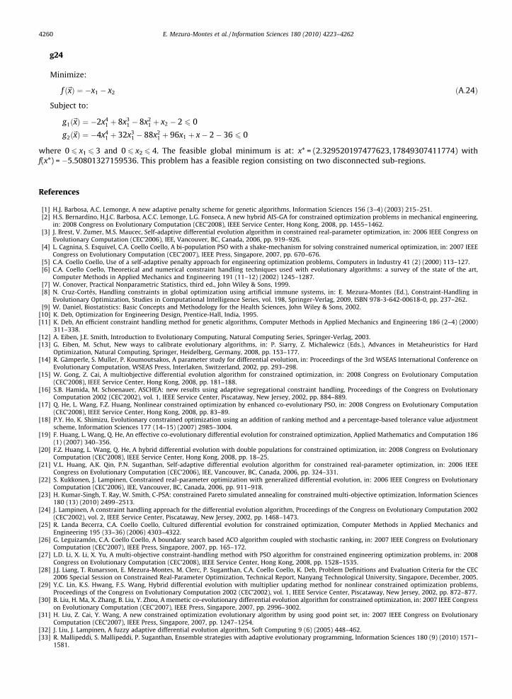
4260 E. Mezura-Montes et al. / Information Sciences 180 (2010) 4223–4262
g24
Minimize:
f ð~xÞ ¼ �x1 � x2 ðA:24Þ
Subject to:
g1ð~xÞ ¼ �2x41 þ 8x3
1 � 8x21 þ x2 � 2 6 0
g2ð~xÞ ¼ �4x41 þ 32x3
1 � 88x21 þ 96x1 þ x� 2� 36 6 0
where 0 6 x1 6 3 and 0 6 x2 6 4. The feasible global minimum is at: x* = (2.329520197477623,17849307411774) withf(x*) = �5.50801327159536. This problem has a feasible region consisting on two disconnected sub-regions.
References
[1] H.J. Barbosa, A.C. Lemonge, A new adaptive penalty scheme for genetic algorithms, Information Sciences 156 (3–4) (2003) 215–251.[2] H.S. Bernardino, H.J.C. Barbosa, A.C.C. Lemonge, L.G. Fonseca, A new hybrid AIS-GA for constrained optimization problems in mechanical engineering,
in: 2008 Congress on Evolutionary Computation (CEC’2008), IEEE Service Center, Hong Kong, 2008, pp. 1455–1462.[3] J. Brest, V. Zumer, M.S. Maucec, Self-adaptive differential evolution algorithm in constrained real-parameter optimization, in: 2006 IEEE Congress on
Evolutionary Computation (CEC’2006), IEE, Vancouver, BC, Canada, 2006, pp. 919–926.[4] L. Cagnina, S. Esquivel, C.A. Coello Coello, A bi-population PSO with a shake-mechanism for solving constrained numerical optimization, in: 2007 IEEE
Congress on Evolutionary Computation (CEC’2007), IEEE Press, Singapore, 2007, pp. 670–676.[5] C.A. Coello Coello, Use of a self-adaptive penalty approach for engineering optimization problems, Computers in Industry 41 (2) (2000) 113–127.[6] C.A. Coello Coello, Theoretical and numerical constraint handling techniques used with evolutionary algorithms: a survey of the state of the art,
Computer Methods in Applied Mechanics and Engineering 191 (11–12) (2002) 1245–1287.[7] W. Conover, Practical Nonparametric Statistics, third ed., John Wiley & Sons, 1999.[8] N. Cruz-Cortés, Handling constraints in global optimization using artificial immune systems, in: E. Mezura-Montes (Ed.), Constraint-Handling in
Evolutionary Optimization, Studies in Computational Intelligence Series, vol. 198, Springer-Verlag, 2009, ISBN 978-3-642-00618-0, pp. 237–262.[9] W. Daniel, Biostatistics: Basic Concepts and Methodology for the Health Sciences, John Wiley & Sons, 2002.
[10] K. Deb, Optimization for Engineering Design, Prentice-Hall, India, 1995.[11] K. Deb, An efficient constraint handling method for genetic algorithms, Computer Methods in Applied Mechanics and Engineering 186 (2–4) (2000)
311–338.[12] A. Eiben, J.E. Smith, Introduction to Evolutionary Computing, Natural Computing Series, Springer-Verlag, 2003.[13] G. Eiben, M. Schut, New ways to calibrate evolutionary algorithms, in: P. Siarry, Z. Michalewicz (Eds.), Advances in Metaheuristics for Hard
Optimization, Natural Computing, Springer, Heidelberg, Germany, 2008, pp. 153–177.[14] R. Gämperle, S. Muller, P. Koumoutsakos, A parameter study for differential evolution, in: Proceedings of the 3rd WSEAS International Conference on
Evolutionary Computation, WSEAS Press, Interlaken, Switzerland, 2002, pp. 293–298.[15] W. Gong, Z. Cai, A multiobjective differential evolution algorithm for constrained optimization, in: 2008 Congress on Evolutionary Computation
(CEC’2008), IEEE Service Center, Hong Kong, 2008, pp. 181–188.[16] S.B. Hamida, M. Schoenauer, ASCHEA: new results using adaptive segregational constraint handling, Proceedings of the Congress on Evolutionary
Computation 2002 (CEC’2002), vol. 1, IEEE Service Center, Piscataway, New Jersey, 2002, pp. 884–889.[17] Q. He, L. Wang, F.Z. Huang, Nonlinear constrained optimization by enhanced co-evolutionary PSO, in: 2008 Congress on Evolutionary Computation
(CEC’2008), IEEE Service Center, Hong Kong, 2008, pp. 83–89.[18] P.Y. Ho, K. Shimizu, Evolutionary constrained optimization using an addition of ranking method and a percentage-based tolerance value adjustment
scheme, Information Sciences 177 (14–15) (2007) 2985–3004.[19] F. Huang, L. Wang, Q. He, An effective co-evolutionary differential evolution for constrained optimization, Applied Mathematics and Computation 186
(1) (2007) 340–356.[20] F.Z. Huang, L. Wang, Q. He, A hybrid differential evolution with double populations for constrained optimization, in: 2008 Congress on Evolutionary
Computation (CEC’2008), IEEE Service Center, Hong Kong, 2008, pp. 18–25.[21] V.L. Huang, A.K. Qin, P.N. Suganthan, Self-adaptive differential evolution algorithm for constrained real-parameter optimization, in: 2006 IEEE
Congress on Evolutionary Computation (CEC’2006), IEE, Vancouver, BC, Canada, 2006, pp. 324–331.[22] S. Kukkonen, J. Lampinen, Constrained real-parameter optimization with generalized differential evolution, in: 2006 IEEE Congress on Evolutionary
Computation (CEC’2006), IEE, Vancouver, BC, Canada, 2006, pp. 911–918.[23] H. Kumar-Singh, T. Ray, W. Smith, C-PSA: constrained Pareto simulated annealing for constrained multi-objective optimization, Information Sciences
180 (13) (2010) 2499–2513.[24] J. Lampinen, A constraint handling approach for the differential evolution algorithm, Proceedings of the Congress on Evolutionary Computation 2002
(CEC’2002), vol. 2, IEEE Service Center, Piscataway, New Jersey, 2002, pp. 1468–1473.[25] R. Landa Becerra, C.A. Coello Coello, Cultured differential evolution for constrained optimization, Computer Methods in Applied Mechanics and
Engineering 195 (33–36) (2006) 4303–4322.[26] G. Leguizamón, C.A. Coello Coello, A boundary search based ACO algorithm coupled with stochastic ranking, in: 2007 IEEE Congress on Evolutionary
Computation (CEC’2007), IEEE Press, Singapore, 2007, pp. 165–172.[27] L.D. Li, X. Li, X. Yu, A multi-objective constraint-handling method with PSO algorithm for constrained engineering optimization problems, in: 2008
Congress on Evolutionary Computation (CEC’2008), IEEE Service Center, Hong Kong, 2008, pp. 1528–1535.[28] J.J. Liang, T. Runarsson, E. Mezura-Montes, M. Clerc, P. Suganthan, C.A. Coello Coello, K. Deb, Problem Definitions and Evaluation Criteria for the CEC
2006 Special Session on Constrained Real-Parameter Optimization, Technical Report, Nanyang Technological University, Singapore, December, 2005.[29] Y.C. Lin, K.S. Hwang, F.S. Wang, Hybrid differential evolution with multiplier updating method for nonlinear constrained optimization problems,
Proceedings of the Congress on Evolutionary Computation 2002 (CEC’2002), vol. 1, IEEE Service Center, Piscataway, New Jersey, 2002, pp. 872–877.[30] B. Liu, H. Ma, X. Zhang, B. Liu, Y. Zhou, A memetic co-evolutionary differential evolution algorithm for constrained optimization, in: 2007 IEEE Congress
on Evolutionary Computation (CEC’2007), IEEE Press, Singapore, 2007, pp. 2996–3002.[31] H. Liu, Z. Cai, Y. Wang, A new constrained optimization evolutionary algorithm by using good point set, in: 2007 IEEE Congress on Evolutionary
Computation (CEC’2007), IEEE Press, Singapore, 2007, pp. 1247–1254.[32] J. Liu, J. Lampinen, A fuzzy adaptive differential evolution algorithm, Soft Computing 9 (6) (2005) 448–462.[33] R. Mallipeddi, S. Mallipeddi, P. Suganthan, Ensemble strategies with adaptive evolutionary programming, Information Sciences 180 (9) (2010) 1571–
1581.

E. Mezura-Montes et al. / Information Sciences 180 (2010) 4223–4262 4261
[34] E. Mezura-Montes (Ed.), Constraint-Handling in Evolutionary Optimization, Studies in Computational Intelligence, vol. 198, Springer-Verlag, 2009.[35] E. Mezura-Montes, C.A. Coello Coello, Identifying on-line behavior and some sources of difficulty in two competitive approaches for constrained
optimization, 2005 IEEE Congress on Evolutionary Computation (CEC’2005), vol. 2, IEEE Press, Edinburgh, Scotland, 2005, pp. 1477–1484.[36] E. Mezura-Montes, C.A. Coello Coello, A simple multimembered evolution strategy to solve constrained optimization problems, IEEE Transactions on
Evolutionary Computation 9 (1) (2005) 1–17.[37] E. Mezura-Montes, C.A. Coello Coello, Constrained optimization via multiobjective evolutionary algorithms, in: J. Knowles, D. Corne, K. Deb (Eds.),
Multiobjective Problems Solving from Nature: From Concepts to Applications, Natural Computing Series, Springer-Verlag, 2008, ISBN 978-3-540-72963-1, pp. 53–76.
[38] E. Mezura-Montes, C.A. Coello Coello, E.I. Tun-Morales, Simple feasibility rules and differential evolution for constrained optimization, in: Proceedingsof the 3rd Mexican International Conference on Artificial Intelligence (MICAI’2004), Lecture Notes in Artificial Intelligence, vol. 2972, Springer-Verlag,Heidelberg, Germany, 2004, pp. 707–716.
[39] E. Mezura-Montes, J.I. Flores-Mendoza, Improved particle swarm optimization in constrained numerical search spaces, in: R. Chiong (Ed.), Nature-Inspired Algorithms for Optimization, Studies in Computational Intelligence Series, vol. 193, Springer-Verlag, 2009, ISBN 978-3-540-72963-1, pp. 299–332.
[40] E. Mezura-Montes, B.C. López-Ramírez, Comparing bio-inspired algorithms in constrained optimization problems, in: 2007 IEEE Congress onEvolutionary Computation (CEC’2007), IEEE Press, Singapore, 2007, pp. 662–669.
[41] E. Mezura-Montes, M.E. Miranda-Varela, R. del Carmen Gómez-Ramón, Additional Results of the Empirical Study on Differential Evolution inConstrained Numerical Optimization, Technical Report TR-EMM-01-2010, LANIA Educational Center, April, 2010. Available at: <http://www.lania.mx/�emezura/tr-EMM-01-2010.pdf>.
[42] E. Mezura-Montes, A.G. Palomeque-Ortiz, Parameter control in differential evolution for constrained optimization, in: 2009 Congress on EvolutionaryComputation (CEC’2009), IEEE Service Center, Trondheim, Norway, 2009, pp. 1375–1382.
[43] E. Mezura-Montes, J. Velázquez-Reyes, C.A.C. Coello, Promising infeasibility and multiple offspring incorporated to differential evolution forconstrained optimization, in: H.G. Beyer et al. (Eds.), Proceedings of the Genetic and Evolutionary Computation Conference (GECCO’2005), WashingtonDC, USA, vol. 1, ACM Press, New York, 2005, ISBN 1-59593-010-8, pp. 225–232.
[44] E. Mezura-Montes, J. Velázquez-Reyes, C.A. Coello Coello, Comparing differential evolution models for global optimization, in: 2006 Genetic andEvolutionary Computation Conference (GECCO’2006), vol. 1, pp. 485–492.
[45] E. Mezura-Montes, J. Velázquez-Reyes, C.A. Coello Coello, Modified differential evolution for constrained optimization, in: 2006 IEEE Congress onEvolutionary Computation (CEC’2006), IEE, Vancouver, BC, Canada, 2006, pp. 332–339.
[46] Z. Michalewicz, M. Schoenauer, Evolutionary algorithms for constrained parameter optimization problems, Evolutionary Computation 4 (1) (1996) 1–32.
[47] A.E. Muñoz-Zavala, A. Hernández-Aguirre, E.R. Villa-Diharce, S. Botello-Rionda, PESO+ for constrained optimization, in: 2006 IEEE Congress onEvolutionary Computation (CEC’2006), IEE, Vancouver, BC, Canada, 2006, pp. 935–942.
[48] A. Oyama, K. Shimoyama, K. Fujii, New constraint-handling method for multi-objective and multi-constraint evolutionary optimization, Transactionsof the Japan Society for Aeronautical and Space Sciences 50 (167) (2007) 56–62.
[49] A.I. Oyman, K. Deb, H.G. Beyer, An alternative constraint handling method for evolution strategies, Proceedings of the Congress on EvolutionaryComputation 1999 (CEC’99), vol. 1, IEEE Service Center, Piscataway, New Jersey, 1999, pp. 612–619.
[50] K. Price, R. Storn, J. Lampinen, Differential Evolution: A Practical Approach to Global Optimization, Natural Computing Series, Springer-Verlag, 2005.[51] K.V. Price, J.I. Rönkkönen, Comparing the uni-modal scaling performance of global and local selection in a mutation-only differential evolution
algorithm, in: 2006 IEEE Congress on Evolutionary Computation (CEC’2006), IEEE Press, Vancouver, Canada, 2006, pp. 7387–7394.[52] T.P. Runarsson, X. Yao, Stochastic ranking for constrained evolutionary optimization, IEEE Transactions on Evolutionary Computation 4 (3) (2000) 284–
294.[53] A.E. Smith, D.W. Coit, Constraint handling techniques—penalty functions, in: T. Bäck, D.B. Fogel, Z. Michalewicz (Eds.), Handbook of Evolutionary
Computation, Oxford University Press, Institute of Physics Publishing, 1997. pp. C 5.2:1–C 5.2:6.[54] T. Takahama, S. Sakai, Constrained optimization by the � constrained differential evolution with gradient-based mutation and feasible elites, in: 2006
IEEE Congress on Evolutionary Computation (CEC’2006), IEE, Vancouver, BC, Canada, 2006, pp. 308–315.[55] T. Takahama, S. Sakai, Constrained optimization by � constrained differential evolution with dynamic �-level control, in: U.K. Chakraborty (Ed.),
Advances in Differential Evolution, Springer, Berlin, 2008, ISBN 978-3-540-68827-3, pp. 139–154.[56] T. Takahama, T. Sakai, Solving difficult constrained optimization problems by the � constrained differential evolution with gradient-based mutation, in:
E. Mezura-Montes (Ed.), Constraint-Handling in Evolutionary Optimization, Studies in Computational Intelligence Series, vol. 198, Springer-Verlag,2009, ISBN 978-3-642-00618-0, pp. 51–72.
[57] M.F. Tasgetiren, P.N. Suganthan, A multi-populated differential evolution algorithm for solving constrained optimization problems, in: 2006 IEEECongress on Evolutionary Computation (CEC’2006), IEE, Vancouver, BC, Canada, 2006, pp. 340–354.
[58] B. Tessema, G.G. Yen, A self-adaptive penalty function based algorithm for constrained optimization, in: 2006 IEEE Congress on EvolutionaryComputation (CEC’2006), IEEE, Vancouver, BC, Canada, 2006, pp. 950–957.
[59] A.S.S.M.B. Ullah, R. Sarker, D. Cornforth, C. Lokan, An agent-based memetic algorithm (AMA) for solving constrained optimization problems, in: 2007IEEE Congress on Evolutionary Computation (CEC’2007), IEEE Press, Singapore, 2007, pp. 999–1006.
[60] B.W. Wah, T. Wang, Y. Shang, Z. Wu, Improving the performance of weighted Lagrange-multiplier methods for nonlinear constrained optimization,Information Sciences 124 (1–4) (2000) 241–272.
[61] Y. Wang, Z. Cai, G. Guo, Y. Zhou, Multiobjective optimization and hybrid evolutionary algorithm to solve constrained optimization problems, IEEETransactions on Systems, Man and Cybernetics Part B – Cybernetics 37 (3) (2007) 560–575.
[62] Y. Wang, Z. Cai, Y. Zhou, Z. Fan, Constrained optimization based on hybrid evolutionary algorithm and adaptive constraint-handling technique,Structural and Multidisciplinary Optimization 37 (4) (2009) 395–413.
[63] Y. Wang, Z. Cai, Y. Zhou, W. Zeng, An adaptive tradeoff model for constrained evolutionary optimization, IEEE Transactions on EvolutionaryComputation 12 (1) (2008) 80–92.
[64] Y. Wang, H. Liu, Z. Cai, Y. Zhou, An orthogonal design based constrained evolutionary optimization algorithm, Engineering Optimization 39 (6) (2007)715–736.
[65] E.F. Wanner, F.G. Guimaraes, R.H.C. Takahashi, P.J. Flemming, Local search with quadratic approximation in genetic algorithms for expensiveoptimization problems, in: 2007 IEEE Congress on Evolutionary Computation (CEC’2007), IEEE Press, Singapore, 2007, pp. 677–683.
[66] D.H. Wolpert, W.G. Macready, No free lunch theorems for optimization, IEEE Transactions on Evolutionary Computation 1 (1) (1997) 67–82.[67] J. Xiao, J. Xu, Z. Shao, C. Jiang, L. Pan, A genetic algorithm for solving multi-constrained function optimization problems based on ks function, in: 2007
IEEE Congress on Evolutionary Computation (CEC’2007), IEEE Press, Singapore, 2007, pp. 4497–4501.[68] Y. Yu, Z.H. Zhou, On the usefulness of infeasible solutions in evolutionary search: a theoretical study, in: 2008 Congress on Evolutionary Computation
(CEC’2008), IEEE Service Center, Hong Kong, 2008, pp. 835–840.[69] S. Zeng, H. Shi, H. Li, G. Chen, L. Ding, L. Kang, A lower-dimensional-search evolutionary algorithm and its application in constrained optimization
problem, in: 2007 IEEE Congress on Evolutionary Computation (CEC’2007), IEEE Press, Singapore, 2007, pp. 1255–1260.[70] M. Zhang, W. Luo, X. Wang, Differential evolution with dynamic stochastic selection for constrained optimization, Information Sciences 178 (15)
(2008) 3043–3074.[71] Q. Zhang, S. Zeng, R. Wang, H. Shi, G. Chen, L. Ding, L. Kang, Constrained optimization by the evolutionary algorithm with lower dimensional crossover
and gradient-based mutation, in: 2008 Congress on Evolutionary Computation (CEC’2008), IEEE Service Center, Hong Kong, 2008, pp. 273–279.

4262 E. Mezura-Montes et al. / Information Sciences 180 (2010) 4223–4262
[72] Y. Zhou, J. He, A runtime analysis of evolutionary algorithms for constrained optimization problems, IEEE Transactions on Evolutionary Computation11 (5) (2007) 608–619.
[73] K. Zielinski, R. Laur, Constrained single-objective optimization using differential evolution, in: 2006 IEEE Congress on Evolutionary Computation(CEC’2006), IEEE, Vancouver, BC, Canada, 2006, pp. 927–934.
[74] K. Zielinski, R. Laur, Stopping criteria for differential evolution in constrained single-objective optimization, in: U.K. Chakraborty (Ed.), Advances inDifferential Evolution, Springer, Berlin, 2008, ISBN 978-3-540-68827-3. pp. 111–138.
[75] K. Zielinski, S.P. Vudathu, R. Laur, Influence of different deviations allowed for equality constraints on particle swarm optimization and differentialevolution, in: N. Krasnogor, G. Nicosia, M. Pavone, D. Pelta (Eds.), Nature Inspired Cooperative Strategies for Optimization, Springer, Berlin, 2008, ISBN978-3-540-78986-4, pp. 249–259.
[76] K. Zielinski, X. Wang, R. Laur, Comparison of adaptive approaches for differential evolution, in: G. Rudolph, T. Jansen, S. Lucas, C. Poloni, N. Beume(Eds.), Parallel Problem Solving from Nature–PPSN X, Lecture Notes in Computer Science, vol. 5199, Springer, Dortmund, Germany, 2008, pp. 641–650.