DIFFRACTION OF SOUND WAVES BY AN APERTURE

IN AN ACOUSTIC BAFFLE

by

J. Isaac Fjeldsted

Advisor

Dr. Scott Sommerfeldt

A Capstone Research Paper submitted to the faculty of

Brigham Young University

in fulfillment of the requirements for the degree of

Bachelor of Science

Physics 492R

Department of Physics and Astronomy

Brigham Young University

August 2008

ABSTRACT

DIFFRACTION OF SOUND WAVES BY AN APERTURE

IN AN ACOUSTIC BAFFLE

J. Isaac Fjeldsted

Department of Physics and Astronomy

Bachelor of Science

In recent years there has been a greater demand in industry for noise control on large

construction vehicles. The Brigham Young University Acoustics Group has been contracted to reexamine insertion loss equations that are currently being used to model the sound field from engine enclosures of these types of vehicles. It has been hypothesized that inaccuracies in the model are partly due to the fact that diffraction is not considered. A numerical model of simple diffraction by an aperture has been created and needs to be tested for accuracy. The purpose of this research is to gather experimental data in order to assess how well this model predicts actual diffracted sound fields from an aperture. Error analysis between experimental and predicted data shows that the numerical model being tested is accurate within a tolerance of ± 4 dB. Research indicates that this model of diffraction may be used in further research to understand insertion loss of engine enclosures.

ii

ACKNOWLEDGEMENTS I would like to express deep gratitude to the following individuals who have guided me through this research and given me support through the entire process: Buye Xu deserves recognition for creating the numerical model that I tested, for his

long hours with me taking measurements, for helping make the plots included in this paper, and for helping me gain a greater understanding of the physical principles behind the acoustical phenomena we observed. He has been a great help to me, and I would not have been able to do this project without his help and his previous work.

Dr. Scott Sommerfeldt gave needed guidance regularly throughout the data gathering process and during the time of writing. His editing helped polish this paper to make it precise and professional. Despite a very busy schedule, he made time when deadlines were tight.

My wife Heidi was patient and loving when this project was most time consuming. She always helps me want to do my best and be positive about my abilities.

iii

TABLE OF CONTENTS

1. BACKGROUND MOTIVATION................................................................................................. 1 2. THEORETICAL FOUNDATION AND PURPOSE.......................................................................... 1 2.1 Enclosures and Insertion loss..................................................................................... 1 2.2 Aims of Present Research............................................................................................ 1 2.3 Theoretical Description of Diffraction........................................................................ 2 2.4 Diffraction by an Aperture.......................................................................................... 2 3. EXPERIMENTAL METHODS................................................................................................... 3 3.1 Measurement Environment/Baffle............................................................................... 3 3.2 Setup............................................................................................................................ 4 3.3 Measurement Techniques............................................................................................ 5 4. DATA AND ANALYSIS........................................................................................................... 5 4.1 Coherence Data............................................................................................................ 6 4.2 Circular Aperture......................................................................................................... 7 4.3 Square Aperture........................................................................................................... 10 4.4 Rectangular Aperture 1................................................................................................ 11 4.5 Rectangular Aperture 2................................................................................................ 12 4.6 Error Analysis.............................................................................................................. 13 5. CONCLUSION......................................................................................................................... 15 REFERENCES.............................................................................................................................. 16

iv

1. BACKGROUND MOTIVATION

For the past decade manufacturers of construction equipment have dealt more intensely with reducing noise emissions from their vehicles. Many cities, states, and countries have noise ordinances that require all activities to be below a predetermined sound pressure level (SPL) during certain parts of the day or in certain areas. Manufacturers must comply to avoid fines or restrictions.

One of these large companies has worked previously with the Acoustics Research Group (ARG) at Brigham Young University to make their vehicles quieter. The objective of the most recent collaboration is to better understand the radiation of sound from engine enclosures of large construction machinery. Design equations for sound from engine enclosures have already been developed by the company, but these equations are not as accurate as desired. The task of the ARG is to modify these design equations and develop a more accurate model that can still be used easily by design engineers who have limited understanding of the underlying acoustics.

2. THEORETICAL FOUNDATION AND PURPOSE 2.1 Enclosures and Insertion loss

The proposed model of the ARG is designed to better predict the insertion loss (IL) of an engine enclosure. In acoustics, insertion loss is the difference between SPL before an element has been added to the system and the SPL after the element has been added as measured at a chosen point outside the enclosure: IL = SPLbefore-SPLafter.1 For the present problem, the engine, fans, and pumps make up the source, and the engine enclosure is the element being added to the system to increase IL.

When actual engine enclosures in practical situations are considered, there are many factors that determine the nature of the sound field outside the enclosure: shape of the enclosure, configuration of sound sources inside the enclosure, size and shape of air intakes, frequency range of the sound produced from various sources, reverberation effects inside the enclosure, vibration of the enclosure walls due to interaction with the air or vibrating parts, etc.2, 3, 4 It would be quite difficult to take all of these different effects into account, and efforts in the past to study enclosure acoustics and IL have focused only on the effects that seem most important.

Beranek describes how to reduce machine produced noise by various means.3 Air-tight

enclosures are the most effective way to reduce unwanted noise from loud machinery. The biggest problem with this approach when engines of construction equipment are considered, is that it does not allow holes or vents for air intake or exhaust. Even a small hole in an enclosure can leak a considerable amount of sound. 2.2 Aims of Present Research

The presence of vents and ducts in engine enclosures has raised the question of how

diffraction of the interior field through these openings affects IL. Up to this point, the

- 1 -

manufacturer’s IL equations have not considered diffraction. The hypothesis of the ARG is that a model including diffraction would be more accurate at predicting IL than the old model.

Background research on diffraction of sound by an aperture is the first step toward finding

out if diffraction ought to be considered in the design model. Buye Xu, a doctoral candidate in the ARG, has created a numerical model of diffraction by an aperture from a simple source behind an infinite baffle. The purpose of the research reported here is to collect data from tests of a physical baffle and a simple speaker source to determine whether the numerical model matches experimental measurements. 2.3 Theoretical Description of Diffraction

At its most basic level diffraction can be thought of as the “bending” of waves around obstacles. This is why we can hear someone yell to us from another room in the house even though the direct path from the other person’s mouth to our ears is obstructed. The phenomenon of sound travelling around corners gives us the impression that sound waves are bent, which is helpful, but a different description of diffraction would be more conducive to this research.

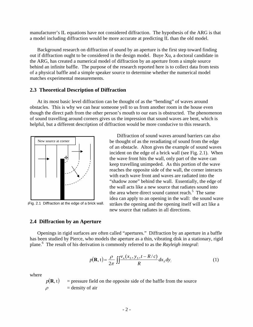
Diffraction of sound waves around barriers can also

be thought of as the reradiating of sound from the edge of an obstacle. Alton gives the example of sound waves incident on the edge of a brick wall (see Fig. 2.1). When the wave front hits the wall, only part of the wave can keep travelling unimpeded. As this portion of the wave reaches the opposite side of the wall, the corner interacts with each wave front and waves are radiated into the “shadow zone” behind the wall. Essentially, the edge of the wall acts like a new source that radiates sound into the area where direct sound cannot reach.5 The same idea can apply to an opening in the wall: the sound wave strikes the opening and the opening itself will act like a new source that radiates in all directions.

gFig. 2.1 Diffraction at the edge of a brick wall.

New source at corner

2.4 Diffraction by an Aperture

Openings in rigid surfaces are often called “apertures.” Diffraction by an aperture in a baffle has been studied by Pierce, who models the aperture as a thin, vibrating disk in a stationary, rigid plane.6 The result of his derivation is commonly referred to as the Rayleigh integral:

( ) ∫∫

−= SS

SSn dydxR

cRtyxvp

)/,,(2

t,πρR (1)

where

( ) t,Rp = pressure field on the opposite side of the baffle from the source ρ = density of air

- 2 -

R = distance from a point ( ) on the disk to a field point SS yx ,c = speed of sound

= velocity (normal) of the disk ),,( tyxv SSn

To more fully understand this equation, imagine a large, solid screen with a circular hole in it of surface area S positioned in the x-y plane. The disk vibrates in the z-direction, so — the velocity of the disk — is considered to be normal to the surface S. The double integral is a surface integral over each point ( ) in S, which calculates the contribution of each point on the disk to the pressure field at the field point R.

nv

SS yx ,( t,Rp )

Just as in the brick wall example, we think of the aperture as a “new source” that radiates

sound into the area on the other side of a baffle. Pierce’s method of assuming disk-like behavior from the aperture is a valid approach that helps to give a better understanding of how sound travels through apertures.

The theoretical model to be verified in this research is based on the Rayleigh integral and logic similar to Pierce’s. As mentioned earlier, Buye Xu of the ARG has created a numerical model that predicts the sound field from an aperture. His model treats the problem similarly to the vibrating disk with a known normal velocity, but on a smaller scale.

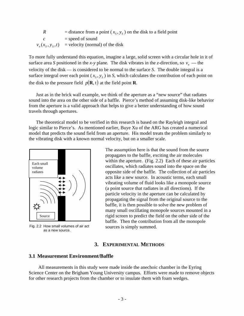
The assumption here is that the sound from the source propagates to the baffle, exciting the air molecules within the aperture. (Fig. 2.2) Each of these air particles oscillates, which radiates sound into the space on the opposite side of the baffle. The collection of air particles acts like a new source. In acoustic terms, each small vibrating volume of fluid looks like a monopole source (a point source that radiates in all directions). If the particle velocity in the aperture can be calculated by propagating the signal from the original source to the baffle, it is then possible to solve the new problem of many small oscillating monopole sources mounted in a rigid screen to predict the field on the other side of the baffle. Then the contribution from all the monopole sources is simply summed.

Fig. 2.2 How small volumes of air act as a new source.

Source

Each small volume radiates

3. EXPERIMENTAL METHODS

3.1 Measurement Environment/Baffle

All measurements in this study were made inside the anechoic chamber in the Eyring Science Center on the Brigham Young University campus. Efforts were made to remove objects for other research projects from the chamber or to insulate them with foam wedges.

- 3 -

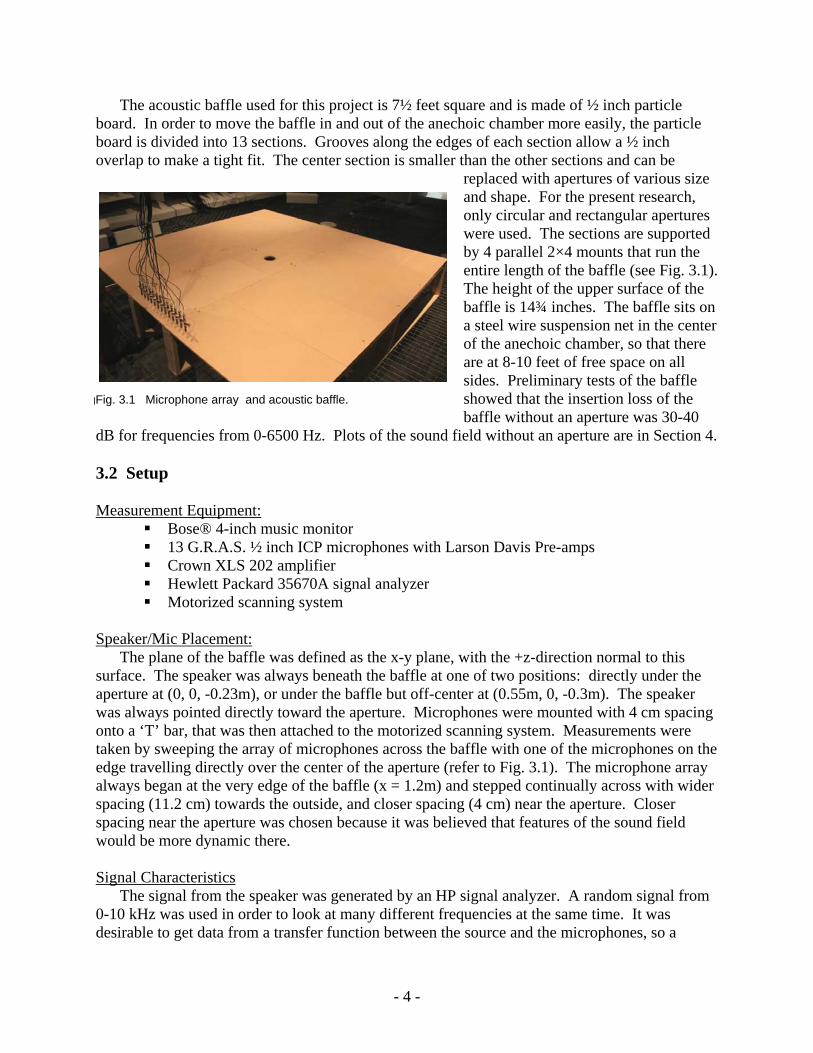
The acoustic baffle used for this project is 7½ feet square and is made of ½ inch particle board. In order to move the baffle in and out of the anechoic chamber more easily, the particle board is divided into 13 sections. Grooves along the edges of each section allow a ½ inch overlap to make a tight fit. The center section is smaller than the other sections and can be

replaced with apertures of various size and shape. For the present research, only circular and rectangular apertures were used. The sections are supported by 4 parallel 2×4 mounts that run the entire length of the baffle (see Fig. 3.1). The height of the upper surface of the baffle is 14¾ inches. The baffle sits on a steel wire suspension net in the center of the anechoic chamber, so that there are at 8-10 feet of free space on all sides. Preliminary tests of the baffle showed that the insertion loss of the baffle without an aperture was 30-40

dB for frequencies from 0-6500 Hz. Plots of the sound field without an aperture are in Section 4.

gFig. 3.1 Microphone array and acoustic baffle.

3.2 Setup Measurement Equipment:

Bose® 4-inch music monitor 13 G.R.A.S. ½ inch ICP microphones with Larson Davis Pre-amps Crown XLS 202 amplifier Hewlett Packard 35670A signal analyzer Motorized scanning system

Speaker/Mic Placement:

The plane of the baffle was defined as the x-y plane, with the +z-direction normal to this surface. The speaker was always beneath the baffle at one of two positions: directly under the aperture at (0, 0, -0.23m), or under the baffle but off-center at (0.55m, 0, -0.3m). The speaker was always pointed directly toward the aperture. Microphones were mounted with 4 cm spacing onto a ‘T’ bar, that was then attached to the motorized scanning system. Measurements were taken by sweeping the array of microphones across the baffle with one of the microphones on the edge travelling directly over the center of the aperture (refer to Fig. 3.1). The microphone array always began at the very edge of the baffle (x = 1.2m) and stepped continually across with wider spacing (11.2 cm) towards the outside, and closer spacing (4 cm) near the aperture. Closer spacing near the aperture was chosen because it was believed that features of the sound field would be more dynamic there. Signal Characteristics

The signal from the speaker was generated by an HP signal analyzer. A random signal from 0-10 kHz was used in order to look at many different frequencies at the same time. It was desirable to get data from a transfer function between the source and the microphones, so a

- 4 -

reference signal was taken directly from the analyzer. The amplifier powering the speaker was kept at the same level for all measurements, so that the transfer function data for each trial could easily be compared. 3.3 Measurement Techniques Measuring the Transfer Function

All plots included here are of the acoustic transfer function between the measurement microphone signals and the input signal. On a very basic level, the transfer function is simply the ratio of the electrical signal (in V or mV) from the HP analyzer to the electrical signal from each microphone in the array (in V or mV). Measured and predicted plots are converted to a logarithmic (dB) scale so that they can be easily compared to sound pressure measurements. Although these plots have values that go below 0 dB, the patterns of the plots and the relative maximum to minimum scales of the plots can be directly compared to actual sound pressure measurements. Coherence

Diffraction measurements in an anechoic environment made it necessary to collect coherence data. Coherence values range from 0 to 1, and are a check to see if two signals have a linear, causal relationship. If a causal relationship with no extraneous noise exists, the coherence will be exactly 1. For the present research, the coherence should have been close to 1 since there was only one source being measured. Coherence plots that were not close to 1 for any frequency mean that a microphone is picking up some foreign source or has a non-linear response. Looking at coherence plots was a way to ensure that only the sound from the important source is being measured.

Subtraction Method: Compensation for baffle effects

Predicted plots generated by the numerical model of diffraction by the aperture assume an infinitely large and infinitely rigid baffle. The sound field produced with the model comes only from the aperture. With a baffle of finite size and finite rigidity, sound was able to diffract around the edges of the baffle and even transmit through the baffle itself. Scans of the baffle with no aperture show these effects quite clearly with peaks and dips that have no distinct pattern. (see Section 4 for plots of the response for a baffle without an aperture) Measurements with an aperture also exhibited very similar peaks and dips, so a “subtraction method” was used to filter out some of the finite baffle effects. The data from the measurements for a baffle without an aperture were simply subtracted, point-by-point, from the measurements with an aperture. As can be seen in the next section, plots with an aperture are much cleaner when this method is used.

4. DATA AND ANALYSIS

All of the following data, with the exception of coherence plots, are on a logarithmic (dB)

scale. As explained in the previous section, all plots of the sound field were generated using the transfer function between input and output signals. Also, rather than scanning the center of the microphone array across the center of the aperture, the first microphone was scanned across the center of the aperture. This was possible because of symmetry on both sides of the y-axis. This

- 5 -

allowed more of the sound field from the center of the aperture into the +y direction to be viewed. Comparison of the numerical model with experimental results is at the end of this section. 4.1 Coherence Data

The coherence of all microphone channels at every measurement position was recorded to

make sure a pure signal was received at each channel. Coherence data were generated for all 13 channels for frequencies of 800 Hz, 850 Hz, 900 Hz, 950 Hz, 1000 Hz, 1050 Hz, and 1100 Hz. Coherence for 900 Hz was very poor (~0.5), so all data for this frequency was not considered. Although coherence was good for the other frequencies, an interesting difference between coherence of measurements with and without an aperture is shown in figures 4.1 and 4.2.

Coh

oere

nce

x-direction across baffle (m)

Fig. 4.1 Typical coherence plot for scan with aperture.

As can been seen, the coherence for both configurations is good. Both exhibit dips at isolated measurement points, but are generally close to 1. It is also clear that the coherence for the scan with an aperture (Fig. 4.1) is closer to 1 than the scan without an aperture (Fig 4.2). This stands to reason since the overall sound level being measured from the source has a smaller magnitude with no aperture. Lower overall sound levels at the receiver allow noise to contaminate sound from the source.

One other interesting thing to

note is that the “no aperture” coherence is worse in the middle of the baffle (around x = 0) because this is when the source signal is weakest. At x = ± 1.12m the coherence is best because of diffraction around the edges of the baffle.

Coh

oere

nce

x-direction across baffle (m)

Fig. 4.2 Typical coherence plot for scan without aperture.

These plots are representative

of coherence for all measurements. Some are better and some are worse than these, but all are close enough to 1 that data were assumed to be accurate.

- 6 -

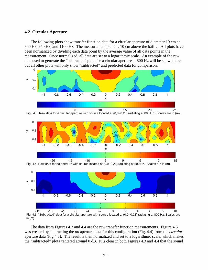
4.2 Circular Aperture The following plots show transfer function data for a circular aperture of diameter 10 cm at 800 Hz, 950 Hz, and 1100 Hz. The measurement plane is 10 cm above the baffle. All plots have been normalized by dividing each data point by the average value of all data points in the measurement. Once normalized, all data are set to a logarithmic scale. An example of the raw data used to generate the “subtracted” plots for a circular aperture at 800 Hz will be shown here, but all other plots will only show “subtracted” and predicted data for comparison. y

Fig. 4.3 Raw data for a circular aperture with source located at (0,0,-0.23) radiating at 800 Hz. Scales are in (m).

y

Fig. 4.4 Raw data for no aperture with source located at (0,0,-0.23) radiating at 800 Hz. Scales are in (m).

y

Fig. 4.5 “Subtracted” data for a circular aperture with source located at (0,0,-0.23) radiating at 800 Hz. Scales are in (m).

The data from Figures 4.3 and 4.4 are the raw transfer function measurements. Figure 4.5

was created by subtracting the no aperture data for this configuration (Fig. 4.4) from the circular aperture data (Fig 4.3). The result is then normalized and set to a logarithmic scale, which makes the “subtracted” plots centered around 0 dB. It is clear in both Figures 4.3 and 4.4 that the sound

- 7 -

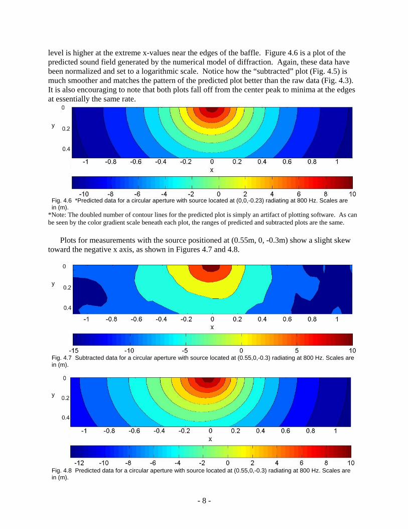
level is higher at the extreme x-values near the edges of the baffle. Figure 4.6 is a plot of the predicted sound field generated by the numerical model of diffraction. Again, these data have been normalized and set to a logarithmic scale. Notice how the “subtracted” plot (Fig. 4.5) is much smoother and matches the pattern of the predicted plot better than the raw data (Fig. 4.3). It is also encouraging to note that both plots fall off from the center peak to minima at the edges at essentially the same rate. y

Fig. 4.6 *Predicted data for a circular aperture with source located at (0,0,-0.23) radiating at 800 Hz. Scales are in (m).

*Note: The doubled number of contour lines for the predicted plot is simply an artifact of plotting software. As can be seen by the color gradient scale beneath each plot, the ranges of predicted and subtracted plots are the same.

Plots for measurements with the source positioned at (0.55m, 0, -0.3m) show a slight skew toward the negative x axis, as shown in Figures 4.7 and 4.8.

y

Fig. 4.7 Subtracted data for a circular aperture with source located at (0.55,0,-0.3) radiating at 800 Hz. Scales are in (m).

y

Fig. 4.8 Predicted data for a circular aperture with source located at (0.55,0,-0.3) radiating at 800 Hz. Scales are in (m).

- 8 -

The skew becomes more apparent with higher frequencies when sound waves are bent even more by diffraction. The following plots are for 1100 Hz.

y

Fig. 4.9 Subtracted data for a circular aperture with source located at (0.55,0,-0.3) radiating at 1100 Hz. Scales are in (m).

y

Fig. 4.10 Predicted data for a circular aperture with source located at (0.55,0,-0.3) radiating at 1100 Hz. Scales are in (m).

As can be seen in Figures 4.9 and 4.10, the increased skew to the sound field is also

accompanied by an increased amount of extraneous noise. Plots of frequencies higher than 1100 Hz became increasingly noisy and sound field patterns were not as easy to see. The following sections contain plots only at 1100 Hz.

- 9 -

4.3 Square Aperture

The square aperture used is 10 cm on a side. Measurements were in a plane 30 cm above the surface of the baffle, so two sweeps of the microphone array were made side-by-side to give a better picture of how the sound field behaves further from the aperture. This makes y-values on plots range from 0 m to 0.96 m. Only plots with the source off-center are shown here so that the skew of diffraction can be seen. Sound waves were incident perpendicular to one side of the square. y

Fig. 4.11 Subtracted data for a square aperture with source located at (0.55,0,-0.3) radiating at 1100 Hz. Scales are in (m).

y

Fig. 4.12 Predicted data for a square aperture with source located at (0.55,0,-0.3) radiating at 1100 Hz. Scales are in (m).

The subtracted plot in figure 4.11 exhibits large dips on the right side. If the general area

around the dips is considered, it is obvious that there is a ~18 dB spread from the peak around (-0.1m, 0) to edge at (1m, 0.9m). This same behavior is seen in the following rectangular plots.

- 10 -

4.4 Rectangular Aperture 1

The measurement plane is the same as for the square aperture. Rectangular apertures used had the same surface area as the square aperture. The aperture from this section has an aspect ratio of 1:1.5, resulting in dimensions of 8.16 cm × 12.25 cm. The source was still positioned at (0.55 m, 0, -0.3m) and the aperture was centered at (0, 0), oriented with its long axis parallel to the y-axis. Sound waves were incident on the long side of the aperture. y

Fig. 4.13 Subtracted data for rectangular aperture 1 (aspect ratio 1:1.5) with source located at (0.55,0,-0.3) radiating at 1100 Hz. Scales are in (m).

y

Fig. 4.14. Predicted data for rectangular aperture 1 (aspect ratio 1:1.5) with source located at (0.55,0,-0.3) radiating at 1100 Hz. Scales are in (m).

Skew can be seen in both predicted and subtracted plots just as was seen before with circular

and square apertures, although the difference between this rectangular aperture and the square aperture is not very great. There is approximately a 16 dB spread from the peak (-0.1m, 0) to the edge (1m, 0.9m).

- 11 -

4.5 Rectangular Aperture 2

This measurement has the same configuration as for the previous rectangular aperture. The second rectangular aperture has an aspect ratio of 1:3 and also has a surface area equal to the area of the square aperture, resulting in dimensions of 5.77cm × 17.32cm. Again, sound waves were incident on the long side of the aperture. y

Fig. 4.15 Subtracted data for rectangular aperture 2 (aspect ratio 1:3) with source located at (0.55,0,-0.3) radiating at 1100 Hz. Scales are in (m).

y

Fig. 4.16 Predicted data for rectangular aperture 2 (aspect ratio 1:3) with source located at (0.55,0,-0.3) radiating at 1100 Hz. Scales are in (m).

It is much clearer with rectangular aperture 2 that the sound field is pulled into a more

elongated pattern. The dB spread from the peak (-0.25m, 0) to the edge (1m, 0.9m) is approximately 17dB for both the predicted and subtracted cases.

- 12 -

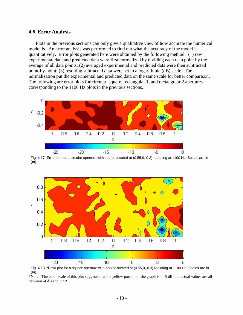
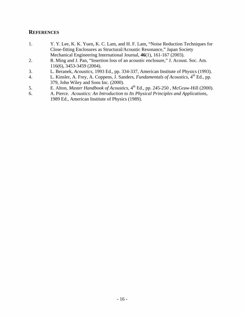
4.6 Error Analysis

Plots in the previous sections can only give a qualitative view of how accurate the numerical model is. An error analysis was performed to find out what the accuracy of the model is quantitatively. Error plots generated here were obtained by the following method: (1) raw experimental data and predicted data were first normalized by dividing each data point by the average of all data points; (2) averaged experimental and predicted data were then subtracted point-by-point; (3) resulting subtracted data were set to a logarithmic (dB) scale. The normalization put the experimental and predicted data on the same scale for better comparison. The following are error plots for circular, square, rectangular 1, and rectangular 2 apertures corresponding to the 1100 Hz plots in the previous sections.

y

Fig. 4.17 Error plot for a circular aperture with source located at (0.55,0,-0.3) radiating at 1100 Hz. Scales are in (m).

y

Fig. 4.18 *Error plot for a square aperture with source located at (0.55,0,-0.3) radiating at 1100 Hz. Scales are in (m).

*Note: The color scale of this plot suggests that the yellow portion of the graph is < -5 dB, but actual values are all between -4 dB and 0 dB.

- 13 -

y

Fig. 4.19 Error plot for rectangular aperture 1 (aspect ratio 1:1.5) with source located at (0.55,0,-0.3) radiating at 1100 Hz. Scales are in (m).

y

Fig. 4.20 Subtracted data for rectangular aperture 2 (aspect ratio 1:3) with source located at (0.55,0,-0.3) radiating at 1100 Hz. Scales are in (m).

The error plots show that there are prominent dips for all measurement configurations on the +x side (the right hand side) of the plot. These dips are quite extreme in Figures 4.17, 4.18, and 4.19. The dips make the range of the plots skew down into large negative numbers, which makes it seem as if the difference between predicted and experimental data is very large. Upon closer inspection, it is clear that over most of the measured area, the difference between predicted and “subtracted” data is less than 4-5 dB. The plot in Figure 4.20 shows a very even spread of error points centered around 0 dB with a spread of only ± 2 dB. If the extreme dips in the other three

- 14 -

plots are disregarded, it can be seen that the data in those plots would also be centered around zero with a spread of 4-5 dB in either direction.

5. CONCLUSION

Experimental data were gathered to assess the accuracy of a numerical model of diffraction by an aperture. Qualitative analysis shows reasonable correlation between experimental and predicted data. Even with noise effects present in the data obtained experimentally, it can be seen that the numerical model predicts the direction and shape of the sound field quite well. A quantitative error analysis was performed by subtracting predicted data from experimental data. It was found that for most points in a plane above the baffle the difference between the numerical model under test and actual sound field measured was less than 4 dB. From the research and evidence presented here, it is believed that this numerical model of diffraction by an aperture is accurate, and that it can be used with confidence when implemented into a larger model for insertion loss of engine enclosures.

- 15 -

REFERENCES

1. Y. Y. Lee, K. K. Yuen, K. C. Lam, and H. F. Lam, “Noise Reduction Techniques for Close-fitting Enclosures as Structural/Acoustic Resonance,” Japan Society Mechanical Engineering International Journal, 46(1), 161-167 (2003).

2. R. Ming and J. Pan, “Insertion loss of an acoustic enclosure,” J. Acoust. Soc. Am. 116(6), 3453-3459 (2004).

3. L. Beranek, Acoustics, 1993 Ed., pp. 334-337, American Institute of Physics (1993). 4. L. Kinsler, A. Frey, A. Coppens, J. Sanders, Fundamentals of Acoustics, 4th Ed., pp.

379, John Wiley and Sons Inc. (2000). 5. E. Alton, Master Handbook of Acoustics, 4th Ed., pp. 245-250 , McGraw-Hill (2000). 6. A. Pierce. Acoustics: An Introduction to Its Physical Principles and Applications,

1989 Ed., American Institute of Physics (1989).

- 16 -