digital communications iii (ece 154c) introduction to...
TRANSCRIPT

1 / 8
Digital Communications III (ECE 154C)
Introduction to Coding and Information Theory
Tara Javidi
These lecture notes were originally developed by late Prof. J. K. Wolf.
UC San Diego
Spring 2014

Overview of ECE 154C
Course Overview
• Course Overview I
• Overview II
Examples
2 / 8

Course Overview I: Digital Communications Block Diagram
Course Overview
• Course Overview I
• Overview II
Examples
3 / 8

Course Overview I: Digital Communications Block Diagram
Course Overview
• Course Overview I
• Overview II
Examples
3 / 8
• Note that the Source Encoder converts all types of information to
a stream of binary digits.

Course Overview I: Digital Communications Block Diagram
Course Overview
• Course Overview I
• Overview II
Examples
3 / 8
• Note that the Source Encoder converts all types of information to
a stream of binary digits.
• Note that the Channel Endcouter, in an attempt to protect the
source coded (binary) stream, judiciously adds redundant bits.

Course Overview I: Digital Communications Block Diagram
Course Overview
• Course Overview I
• Overview II
Examples
3 / 8
• Sometimes the output of the source decoder must be an exact
{replica of the information (e.g. computer data) — called
NOISELESS CODING (aka lossless compression)

Course Overview I: Digital Communications Block Diagram
Course Overview
• Course Overview I
• Overview II
Examples
3 / 8
• Sometimes the output of the source decoder must be an exact
{replica of the information (e.g. computer data) — called
NOISELESS CODING (aka lossless compression)
• Other times the output of the source decoder can be
approximately equal to the information (e.g. music, tv, speech) —
called CODING WITH DISTORTION (aka lossy compression)
Overview II: What will we cover?
Course Overview
• Course Overview I
• Overview II
Examples
4 / 8
REFERENCE: CHAPTER 10 ZIEMER & TRANTER
SOURCE CODING - NOISELESS CODES
◦ Basic idea is to use as few binary digits as possible and still
be able to recover the information exactly
◦ Topics include:
• Huffman Codes
• Shannon Fano Codes
• Tunstall Codes
• Entropy of Source
• Lempel-Ziv Codes

Overview II: What will we cover?
Course Overview
• Course Overview I
• Overview II
Examples
4 / 8
REFERENCE: CHAPTER 10 ZIEMER & TRANTER
SOURCE CODING WITH DISTORTION
◦ Again the idea is to use minimum number of binary digits for a
given value of distortion
◦ Topics include:
• Gaussian Source
• Optimal Quantizing

Overview II: What will we cover?
Course Overview
• Course Overview I
• Overview II
Examples
4 / 8
REFERENCE: CHAPTER 10 ZIEMER & TRANTER
CHANNEL CAPACITY OF A NOISY CHANNEL
◦ Even if channel is noisy, messages can be sent essentially
error free if extra digits are transmitted
◦ Basic idea is to use as few extra digits as possible
◦ Topics Covered:
• Channel Capacity
• Mutual Information
• Some Examples

Overview II: What will we cover?
Course Overview
• Course Overview I
• Overview II
Examples
4 / 8
REFERENCE: CHAPTER 10 ZIEMER & TRANTER
CHANNEL CODING
◦ Basic idea — Detect errors that occured on channel and then
correct them
◦ Topics Covered:
• Hamming Code
• General Theory of Block Codes
(Parity Check Matrix, Generator Matrix, Minimum
Distance, etc.)
• LDPC Codes
• Turbo Codes
• Code Performance

A Few Examples
Course Overview
Examples
• Example 1
• Example 2
• More Examples
5 / 8

Example 1: 4 letter DMS
Course Overview
Examples
• Example 1
• Example 2
• More Examples
6 / 8
Basic concepts came from one paper of one man named
Claude Shannon!

Example 1: 4 letter DMS
Course Overview
Examples
• Example 1
• Example 2
• More Examples
6 / 8
Basic concepts came from one paper of one man named
Claude Shannon! Shannon used simple models that
capture the essence of the problem!

Example 1: 4 letter DMS
Course Overview
Examples
• Example 1
• Example 2
• More Examples
6 / 8
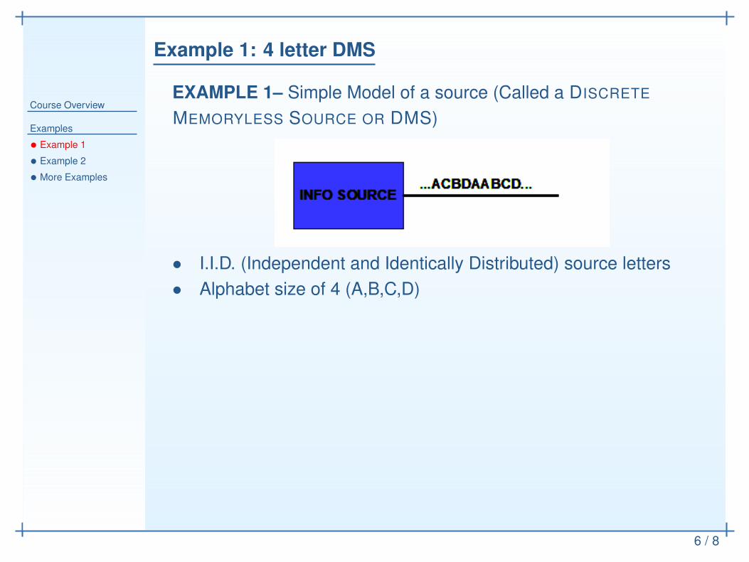
EXAMPLE 1– Simple Model of a source (Called a DISCRETE
MEMORYLESS SOURCE OR DMS)

Example 1: 4 letter DMS
Course Overview
Examples
• Example 1
• Example 2
• More Examples
6 / 8
EXAMPLE 1– Simple Model of a source (Called a DISCRETE
MEMORYLESS SOURCE OR DMS)
• I.I.D. (Independent and Identically Distributed) source letters
Example 1: 4 letter DMS
Course Overview
Examples
• Example 1
• Example 2
• More Examples
6 / 8
EXAMPLE 1– Simple Model of a source (Called a DISCRETE
MEMORYLESS SOURCE OR DMS)
• I.I.D. (Independent and Identically Distributed) source letters
• Alphabet size of 4 (A,B,C,D)

Example 1: 4 letter DMS
Course Overview
Examples
• Example 1
• Example 2
• More Examples
6 / 8
EXAMPLE 1– Simple Model of a source (Called a DISCRETE
MEMORYLESS SOURCE OR DMS)
• I.I.D. (Independent and Identically Distributed) source letters
• Alphabet size of 4 (A,B,C,D)
• P(A) = p1, P(B) = p2, P(C) = p3, P(D) = p4,∑
ipi = 1
• Simplest CodeA −→ 00B −→ 01C −→ 10D −→ 11

Example 1: 4 letter DMS
Course Overview
Examples
• Example 1
• Example 2
• More Examples
6 / 8

Example 1: 4 letter DMS
Course Overview
Examples
• Example 1
• Example 2
• More Examples
6 / 8
• Average length of code words
L = 2(p1 + p2 + p3 + p4) = 2

Example 1: 4 letter DMS
Course Overview
Examples
• Example 1
• Example 2
• More Examples
6 / 8
• Average length of code words
L = 2(p1 + p2 + p3 + p4) = 2
Q: Can we use fewer than 2 binary digits per source letter (on the
average) and still recover information from the binary sequence?

Example 1: 4 letter DMS
Course Overview
Examples
• Example 1
• Example 2
• More Examples
6 / 8
• Average length of code words
L = 2(p1 + p2 + p3 + p4) = 2
Q: Can we use fewer than 2 binary digits per source letter (on the
average) and still recover information from the binary sequence?
A: Depends on values of (p1, p2, p3, p4)

Example 2: Binary Symmetric Channel
Course Overview
Examples
• Example 1
• Example 2
• More Examples
7 / 8
EXAMPLE 2– Simple Model for Noisy Channel

Example 2: Binary Symmetric Channel
Course Overview
Examples
• Example 1
• Example 2
• More Examples
7 / 8
EXAMPLE 2– Simple Model for Noisy Channel
Channels, as you saw in ECE154B, can be viewed as
If s0(t) = −s1(t) and equally likely signals,
Perror = Q
(
√
2E
N0
)
= P

Example 2: Binary Symmetric Channel
Course Overview
Examples
• Example 1
• Example 2
• More Examples
7 / 8
EXAMPLE 2– Simple Model for Noisy Channel
Channels, as you saw in ECE154B, can be viewed as
If s0(t) = −s1(t) and equally likely signals,
Perror = Q
(
√
2E
N0
)
= P
Q: Can we send information “error-free” over such a channel even
though p 6= 0, 1?

Example 2: Binary Symmetric Channel
Course Overview
Examples
• Example 1
• Example 2
• More Examples
7 / 8
EXAMPLE 2– Simple Model for Noisy Channel
Shannon considered a simpler channel called binary symmetric
channel (or BSC for short)
Pictorially Mathematically
PY |X(y|x) =
{
1− p y = x
p y 6= x
Q: Can we send information “error-free” over such a channel even
though p 6= 0, 1?
A: Depends on the rate of transmission (how many channel uses
are allowed per information bit). Essentially for small enough of
transmission rate (to be defined precisely), the answer is YES!

Example 3: DMS with Alphabet size 8
Course Overview
Examples
• Example 1
• Example 2
• More Examples
8 / 8

Example 3: DMS with Alphabet size 8
Course Overview
Examples
• Example 1
• Example 2
• More Examples
8 / 8
EXAMPLE 3– Discrete Memoryless Source with alphabet size of 8
letters: {A,B,C,D,E, F,G,H}
• Probabilities: {pA ≥ pB ≥ pC ≥ pD ≥ pE ≥ pF ≥ pG, pH}• See the following codes:
Q: Which codes are uniquely decodable? Which ones are
instantaneously decodable? Compute the average length of the
codewords for each code.

Example 3: DMS with Alphabet size 8
Course Overview
Examples
• Example 1
• Example 2
• More Examples
8 / 8
EXAMPLE 4– Can you optimally design a code?
L =1
2× 1 +
1
4× 2 +
1
8× 3 +
1
16× 4 +
4
64× 6
=1
32+
1
32+
1
16+
1
8+
1
4+
1
2+ 1 = 2
We will see that this is an optimal code (not only among the
single-letter constructions but overall).

Example 3: DMS with Alphabet size 8
Course Overview
Examples
• Example 1
• Example 2
• More Examples
8 / 8
EXAMPLE 5–
L = .1 + .1 + .2 + .2 + .3 + .5 + 1 = 2.4
But here we can do better by encoding 2 source letters (or more) at a
time?