dimension reduction and component analysis
TRANSCRIPT

Dimension Reduction and Component Analysis
Jason Corso
SUNY at Buffalo
J. Corso (SUNY at Buffalo) Dimension Reduction and Component Analysis 1 / 102

Plan
We learned about estimating parametric models and how these thenform classifiers and define decision boundariesNow we turn back to the question of dimensionality.Recall the fish example, where we experimented with the lengthfeature first, then the lightness feature, and then decided upon acombination of the width and lightness.
salmon sea bass
length
count
l*
0
2
4
6
8
10
12
16
18
20
22
5 10 2015 25
FIGURE 1.2. Histograms for the length feature for the two categories. No single thresh-old value of the length will serve to unambiguously discriminate between the two cat-egories; using length alone, we will have some errors. The value marked l∗ will lead tothe smallest number of errors, on average. From: Richard O. Duda, Peter E. Hart, andDavid G. Stork, Pattern Classification. Copyright c© 2001 by John Wiley & Sons, Inc.
2 4 6 8 100
2
4
6
8
10
12
14
lightness
count
x*
salmon sea bass
FIGURE 1.3. Histograms for the lightness feature for the two categories. No singlethreshold value x∗ (decision boundary) will serve to unambiguously discriminate be-tween the two categories; using lightness alone, we will have some errors. The value x∗
marked will lead to the smallest number of errors, on average. From: Richard O. Duda,Peter E. Hart, and David G. Stork, Pattern Classification. Copyright c© 2001 by JohnWiley & Sons, Inc.
2 4 6 8 1014
15
16
17
18
19
20
21
22
width
lightness
salmon sea bass
FIGURE 1.4. The two features of lightness and width for sea bass and salmon. The darkline could serve as a decision boundary of our classifier. Overall classification error onthe data shown is lower than if we use only one feature as in Fig. 1.3, but there willstill be some errors. From: Richard O. Duda, Peter E. Hart, and David G. Stork, PatternClassification. Copyright c© 2001 by John Wiley & Sons, Inc.
We developed some intuition saying the more features I add, thebetter my classifier will be...
We will see that in theory this may be, but in practice, this is not thecase—the probability of error will increase after a certain number offeatures (dimensionality) has been reached.We will first explore this point and then discuss a set of methods fordimension reduction.
J. Corso (SUNY at Buffalo) Dimension Reduction and Component Analysis 2 / 102

Plan
We learned about estimating parametric models and how these thenform classifiers and define decision boundariesNow we turn back to the question of dimensionality.Recall the fish example, where we experimented with the lengthfeature first, then the lightness feature, and then decided upon acombination of the width and lightness.
salmon sea bass
length
count
l*
0
2
4
6
8
10
12
16
18
20
22
5 10 2015 25
FIGURE 1.2. Histograms for the length feature for the two categories. No single thresh-old value of the length will serve to unambiguously discriminate between the two cat-egories; using length alone, we will have some errors. The value marked l∗ will lead tothe smallest number of errors, on average. From: Richard O. Duda, Peter E. Hart, andDavid G. Stork, Pattern Classification. Copyright c© 2001 by John Wiley & Sons, Inc.
2 4 6 8 100
2
4
6
8
10
12
14
lightness
count
x*
salmon sea bass
FIGURE 1.3. Histograms for the lightness feature for the two categories. No singlethreshold value x∗ (decision boundary) will serve to unambiguously discriminate be-tween the two categories; using lightness alone, we will have some errors. The value x∗
marked will lead to the smallest number of errors, on average. From: Richard O. Duda,Peter E. Hart, and David G. Stork, Pattern Classification. Copyright c© 2001 by JohnWiley & Sons, Inc.
2 4 6 8 1014
15
16
17
18
19
20
21
22
width
lightness
salmon sea bass
FIGURE 1.4. The two features of lightness and width for sea bass and salmon. The darkline could serve as a decision boundary of our classifier. Overall classification error onthe data shown is lower than if we use only one feature as in Fig. 1.3, but there willstill be some errors. From: Richard O. Duda, Peter E. Hart, and David G. Stork, PatternClassification. Copyright c© 2001 by John Wiley & Sons, Inc.
We developed some intuition saying the more features I add, thebetter my classifier will be...We will see that in theory this may be, but in practice, this is not thecase—the probability of error will increase after a certain number offeatures (dimensionality) has been reached.
We will first explore this point and then discuss a set of methods fordimension reduction.
J. Corso (SUNY at Buffalo) Dimension Reduction and Component Analysis 2 / 102

Plan
We learned about estimating parametric models and how these thenform classifiers and define decision boundariesNow we turn back to the question of dimensionality.Recall the fish example, where we experimented with the lengthfeature first, then the lightness feature, and then decided upon acombination of the width and lightness.
salmon sea bass
length
count
l*
0
2
4
6
8
10
12
16
18
20
22
5 10 2015 25
FIGURE 1.2. Histograms for the length feature for the two categories. No single thresh-old value of the length will serve to unambiguously discriminate between the two cat-egories; using length alone, we will have some errors. The value marked l∗ will lead tothe smallest number of errors, on average. From: Richard O. Duda, Peter E. Hart, andDavid G. Stork, Pattern Classification. Copyright c© 2001 by John Wiley & Sons, Inc.
2 4 6 8 100
2
4
6
8
10
12
14
lightness
count
x*
salmon sea bass
FIGURE 1.3. Histograms for the lightness feature for the two categories. No singlethreshold value x∗ (decision boundary) will serve to unambiguously discriminate be-tween the two categories; using lightness alone, we will have some errors. The value x∗
marked will lead to the smallest number of errors, on average. From: Richard O. Duda,Peter E. Hart, and David G. Stork, Pattern Classification. Copyright c© 2001 by JohnWiley & Sons, Inc.
2 4 6 8 1014
15
16
17
18
19
20
21
22
width
lightness
salmon sea bass
FIGURE 1.4. The two features of lightness and width for sea bass and salmon. The darkline could serve as a decision boundary of our classifier. Overall classification error onthe data shown is lower than if we use only one feature as in Fig. 1.3, but there willstill be some errors. From: Richard O. Duda, Peter E. Hart, and David G. Stork, PatternClassification. Copyright c© 2001 by John Wiley & Sons, Inc.
We developed some intuition saying the more features I add, thebetter my classifier will be...We will see that in theory this may be, but in practice, this is not thecase—the probability of error will increase after a certain number offeatures (dimensionality) has been reached.We will first explore this point and then discuss a set of methods fordimension reduction.
J. Corso (SUNY at Buffalo) Dimension Reduction and Component Analysis 2 / 102

Dimensionality
High Dimensions Often Test Our Intuitions
Consider a simple arrangement: youhave a sphere of radius r = 1 in a spaceof D dimensions.
We want to compute what is thefraction of the volume of the spherethat lies between radius r = 1− ε andr = 1.
Noting that the volume of the spherewill scale with rD, we have:
VD(r) = KDrD (1)
where KD is some constant (dependingonly on D).
VD(1)− VD(1− ε)VD(1)
=
1− (1− ε)D(2)
ε
volu
me
frac
tion
D = 1
D = 2
D = 5
D = 20
0 0.2 0.4 0.6 0.8 10
0.2
0.4
0.6
0.8
1
J. Corso (SUNY at Buffalo) Dimension Reduction and Component Analysis 3 / 102
Dimensionality
Let’s Build Some More IntuitionExample from Bishop PRML
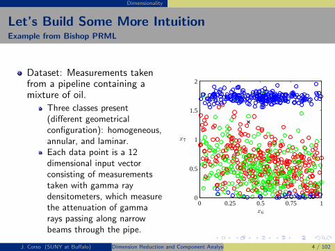
Dataset: Measurements takenfrom a pipeline containing amixture of oil.
Three classes present(different geometricalconfiguration): homogeneous,annular, and laminar.Each data point is a 12dimensional input vectorconsisting of measurementstaken with gamma raydensitometers, which measurethe attenuation of gammarays passing along narrowbeams through the pipe.
x6
x7
0 0.25 0.5 0.75 10
0.5
1
1.5
2
J. Corso (SUNY at Buffalo) Dimension Reduction and Component Analysis 4 / 102

Dimensionality
Let’s Build Some More IntuitionExample from Bishop PRML
100 data points of features x6and x7 are shown on the right.
Goal: Classify the new datapoint at the ‘x’.
Suggestions on how we mightapproach this classificationproblem?
x6
x7
0 0.25 0.5 0.75 10
0.5
1
1.5
2
J. Corso (SUNY at Buffalo) Dimension Reduction and Component Analysis 5 / 102

Dimensionality
Let’s Build Some More IntuitionExample from Bishop PRML
Observations we can make:
The cross is surrounded bymany red points and some greenpoints.
Blue points are quite far fromthe cross.
Nearest-Neighbor Intuition:The query point should bedetermined more strongly bynearby points from the trainingset and less strongly by moredistant points. x6
x7
0 0.25 0.5 0.75 10
0.5
1
1.5
2
J. Corso (SUNY at Buffalo) Dimension Reduction and Component Analysis 6 / 102

Dimensionality
Let’s Build Some More IntuitionExample from Bishop PRML
One simple way of doing it is:
We can divide the feature spaceup into regular cells.
For each, cell, we associated theclass that occurs mostfrequently in that cell (in ourtraining data).
Then, for a query point, wedetermine which cell it falls intoand then assign in the labelassociated with the cell.
What problems may exist withthis approach?
x6
x7
0 0.25 0.5 0.75 10
0.5
1
1.5
2
J. Corso (SUNY at Buffalo) Dimension Reduction and Component Analysis 7 / 102

Dimensionality
Let’s Build Some More IntuitionExample from Bishop PRML
The problem we are most interested in now is the one that becomesapparent when we add more variables into the mix, corresponding toproblems of higher dimensionality.
In this case, the number of additional cells grows exponentially withthe dimensionality of the space.
Hence, we would need an exponentially large training data set toensure all cells are filled.
x1
D = 1x1
x2
D = 2
x1
x2
x3
D = 3
J. Corso (SUNY at Buffalo) Dimension Reduction and Component Analysis 8 / 102

Dimensionality
Curse of Dimensionality
This severe difficulty when working in high dimensions was coined thecurse of dimensionality by Bellman in 1961.
The idea is that the volume of a space increases exponentially withthe dimensionality of the space.
J. Corso (SUNY at Buffalo) Dimension Reduction and Component Analysis 9 / 102
Dimensionality
Dimensionality and Classification Error?Some parts taken from G. V. Trunk, TPAMI Vol. 1 No. 3 PP. 306-7 1979
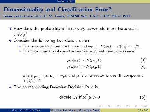
How does the probability of error vary as we add more features, intheory?
Consider the following two-class problem:
The prior probabilities are known and equal: P (ω1) = P (ω2) = 1/2.The class-conditional densities are Gaussian with unit covariance:
p(x|ω1) ∼ N(µ1, I) (3)
p(x|ω2) ∼ N(µ2, I) (4)
where µ1 = µ, µ2 = −µ, and µ is an n-vector whose ith componentis (1/i)1/2.
The corresponding Bayesian Decision Rule is
decide ω1 if xTµ > 0 (5)
J. Corso (SUNY at Buffalo) Dimension Reduction and Component Analysis 10 / 102
Dimensionality
Dimensionality and Classification Error?Some parts taken from G. V. Trunk, TPAMI Vol. 1 No. 3 PP. 306-7 1979
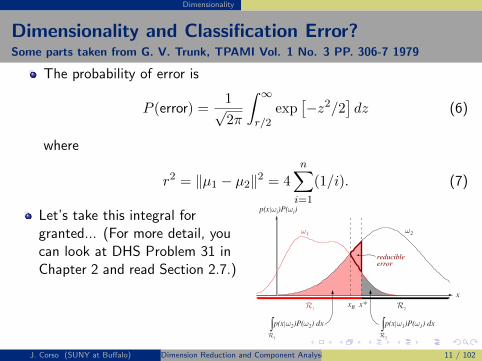
The probability of error is
P (error) =1√2π
∫ ∞
r/2exp
[−z2/2
]dz (6)
where
r2 = ‖µ1 − µ2‖2 = 4
n∑
i=1
(1/i). (7)
Let’s take this integral forgranted... (For more detail, youcan look at DHS Problem 31 inChapter 2 and read Section 2.7.)
What can we say about thisresult as more features areadded?
ω2ω1
x
p(x|ωi)P(ωi)
reducibleerror
∫p(x|ω1)P(ω1) dx∫p(x|ω2)P(ω2) dx
R2R1
R1 R2
xB x*
FIGURE 2.17. Components of the probability of error for equal priors and (nonoptimal)decision point x∗. The pink area corresponds to the probability of errors for deciding ω1
when the state of nature is in fact ω2; the gray area represents the converse, as given inEq. 70. If the decision boundary is instead at the point of equal posterior probabilities,xB, then this reducible error is eliminated and the total shaded area is the minimumpossible; this is the Bayes decision and gives the Bayes error rate. From: Richard O.Duda, Peter E. Hart, and David G. Stork, Pattern Classification. Copyright c© 2001 byJohn Wiley & Sons, Inc.
J. Corso (SUNY at Buffalo) Dimension Reduction and Component Analysis 11 / 102

Dimensionality
Dimensionality and Classification Error?Some parts taken from G. V. Trunk, TPAMI Vol. 1 No. 3 PP. 306-7 1979
The probability of error approaches 0 as n approach infinity because1/i is a divergent series.
More intuitively, each additional feature is going to decrease theprobability of error as long as its means are different. In the generalcase of varying means and but same variance for a feature, we have
r2 =d∑
i=1
(µi1 − µi2
σi
)2
(8)
Certainly, we prefer features that have big differences in the meanrelative to their variance.
We need to note that if the probabilistic structure of the problem iscompletely known then adding new features is not going to decreasethe Bayes risk (or increase it).
J. Corso (SUNY at Buffalo) Dimension Reduction and Component Analysis 12 / 102

Dimensionality
Dimensionality and Classification Error?Some parts taken from G. V. Trunk, TPAMI Vol. 1 No. 3 PP. 306-7 1979
So, adding dimensions is good....
x3
x1
x2
FIGURE 3.3. Two three-dimensional distributions have nonoverlapping densities, andthus in three dimensions the Bayes error vanishes. When projected to a subspace—here,the two-dimensional x1 − x2 subspace or a one-dimensional x1 subspace—there canbe greater overlap of the projected distributions, and hence greater Bayes error. From:Richard O. Duda, Peter E. Hart, and David G. Stork, Pattern Classification. Copyrightc© 2001 by John Wiley & Sons, Inc.
...in theory.
But, in practice, performance seems to not obey this theory.
J. Corso (SUNY at Buffalo) Dimension Reduction and Component Analysis 13 / 102

Dimensionality
Dimensionality and Classification Error?Some parts taken from G. V. Trunk, TPAMI Vol. 1 No. 3 PP. 306-7 1979
Consider again the two-class problem, but this time with unknownmeans µ1 and µ2.
Instead, we have m labeled samples x1, . . . ,xm.
Then, the best estimate of µ for each class is the sample mean (recallthe parameter estimation lecture).
µ =1
m
m∑
i=1
xi (9)
where xi comes from ω2. The covariance matrix is I/m.
J. Corso (SUNY at Buffalo) Dimension Reduction and Component Analysis 14 / 102

Dimensionality
Dimensionality and Classification Error?Some parts taken from G. V. Trunk, TPAMI Vol. 1 No. 3 PP. 306-7 1979
Probablity of error is given by
P (error) = P (xTµ ≥ 0|ω2) =1√2π
∫ ∞
γn
exp[−z2/2
]dz (10)
because it has a Gaussian form as n approaches infinity where
γn = E(z)/ [var(z)]1/2 (11)
E(z) =
n∑
i=1
(1/i) (12)
var(z) =
(1 +
1
m
) n∑
i=1
(1/i) + n/m (13)
J. Corso (SUNY at Buffalo) Dimension Reduction and Component Analysis 15 / 102

Dimensionality
Dimensionality and Classification Error?Some parts taken from G. V. Trunk, TPAMI Vol. 1 No. 3 PP. 306-7 1979
Probablity of error is given by
P (error) = P (xTµ ≥ 0|ω2) =1√2π
∫ ∞
γn
exp[−z2/2
]dz
The key is that we can show
limn→∞
γn = 0 (14)
and thus the probability of error approaches one-half as thedimensionality of the problem becomes very high.
J. Corso (SUNY at Buffalo) Dimension Reduction and Component Analysis 16 / 102

Dimensionality
Dimensionality and Classification Error?Some parts taken from G. V. Trunk, TPAMI Vol. 1 No. 3 PP. 306-7 1979
Trunk performed an experiment to investigate the convergence rate ofthe probability of error to one-half. He simulated the problem fordimensionality 1 to 1000 and ran 500 repetitions for each dimension.We see an increase in performance initially and then a decrease (asthe dimensionality of the problem grows larger than the number oftraining samples).
J. Corso (SUNY at Buffalo) Dimension Reduction and Component Analysis 17 / 102

Dimension Reduction
Motivation for Dimension Reduction
The discussion on the curse of dimensionality should be enough!
Even though our problem may have a high dimension, data will oftenbe confined to a much lower effective dimension in most real worldproblems.
Computational complexity is another important point: generally, thehigher the dimension, the longer the training stage will be (andpotentially the measurement and classification stages).
We seek an understanding of the underlying data to
Remove or reduce the influence of noisy or irrelevant features thatwould otherwise interfere with the classifier;Identify a small set of features (perhaps, a transformation thereof)during data exploration.
J. Corso (SUNY at Buffalo) Dimension Reduction and Component Analysis 18 / 102

Dimension Reduction Principal Component Analysis
Dimension Reduction Version 0
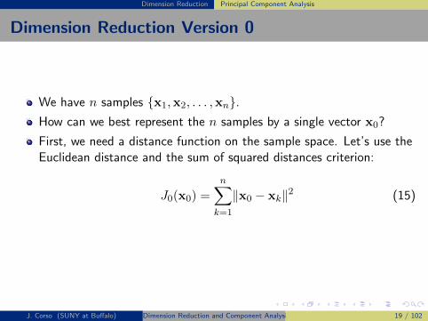
We have n samples {x1,x2, . . . ,xn}.How can we best represent the n samples by a single vector x0?
First, we need a distance function on the sample space. Let’s use theEuclidean distance and the sum of squared distances criterion:
J0(x0) =n∑
k=1
‖x0 − xk‖2 (15)
Then, we seek a value of x0 that minimizes J0.
J. Corso (SUNY at Buffalo) Dimension Reduction and Component Analysis 19 / 102
Dimension Reduction Principal Component Analysis
Dimension Reduction Version 0
We have n samples {x1,x2, . . . ,xn}.How can we best represent the n samples by a single vector x0?
First, we need a distance function on the sample space. Let’s use theEuclidean distance and the sum of squared distances criterion:
J0(x0) =
n∑
k=1
‖x0 − xk‖2 (15)
Then, we seek a value of x0 that minimizes J0.
J. Corso (SUNY at Buffalo) Dimension Reduction and Component Analysis 19 / 102

Dimension Reduction Principal Component Analysis
Dimension Reduction Version 0
We can show that the minimizer is indeed the sample mean:
m =1
n
n∑
k=1
xk (16)
We can verify it by adding m−m into J0:
J0(x0) =
n∑
k=1
‖(x0 −m)− (xk −m)‖2 (17)
=
n∑
k=1
‖x0 −m‖2 +n∑
k=1
‖xk −m‖2 (18)
Thus, J0 is minimized when x0 = m. Note, the second term isindependent of x0.
J. Corso (SUNY at Buffalo) Dimension Reduction and Component Analysis 20 / 102

Dimension Reduction Principal Component Analysis
Dimension Reduction Version 0
So, the sample mean is an initial dimension-reduced representation ofthe data (a zero-dimensional one).
It is simple, but it not does reveal any of the variability in the data.
Let’s try to obtain a one-dimensional representation: i.e., let’s projectthe data onto a line running through the sample mean.
J. Corso (SUNY at Buffalo) Dimension Reduction and Component Analysis 21 / 102

Dimension Reduction Principal Component Analysis
Dimension Reduction Version 1
Let e be a unit vector in the direction of the line.The standard equation for a line is then
x = m+ ae (19)
where scalar a ∈ R governs which point along the line we are andhence corresponds to the distance of any point x from the mean m.
Represent point xk by m+ ake.We can find an optimal set of coefficients by again minimizing thesquared-error criterion
J1(a1, . . . , an, e) =
n∑
k=1
‖(m+ ake)− xk‖2 (20)
=
n∑
k=1
a2k‖e‖2 − 2
n∑
k=1
akeT(xk −m) +
n∑
k=1
‖xk −m‖2
(21)
J. Corso (SUNY at Buffalo) Dimension Reduction and Component Analysis 22 / 102

Dimension Reduction Principal Component Analysis
Dimension Reduction Version 1
Let e be a unit vector in the direction of the line.The standard equation for a line is then
x = m+ ae (19)
where scalar a ∈ R governs which point along the line we are andhence corresponds to the distance of any point x from the mean m.Represent point xk by m+ ake.We can find an optimal set of coefficients by again minimizing thesquared-error criterion
J1(a1, . . . , an, e) =
n∑
k=1
‖(m+ ake)− xk‖2 (20)
=
n∑
k=1
a2k‖e‖2 − 2
n∑
k=1
akeT(xk −m) +
n∑
k=1
‖xk −m‖2
(21)
J. Corso (SUNY at Buffalo) Dimension Reduction and Component Analysis 22 / 102

Dimension Reduction Principal Component Analysis
Dimension Reduction Version 1
Differentiating for ak and equating to 0 yields
ak = eT(xk −m) (22)
This indicates that the best value for ak is the projection of the pointxk onto the line e that passes through m.
How do we find the best direction for that line?
J. Corso (SUNY at Buffalo) Dimension Reduction and Component Analysis 23 / 102
Dimension Reduction Principal Component Analysis
Dimension Reduction Version 1
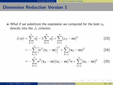
What if we substitute the expression we computed for the best akdirectly into the J1 criterion:
J1(e) =
n∑
k=1
a2k − 2
n∑
k=1
a2k +
n∑
k=1
‖xk −m‖2 (23)
= −n∑
k=1
[eT(xk −m)
]2+
n∑
k=1
‖xk −m‖2 (24)
= −n∑
k=1
eT(xk −m)(xk −m)Te+
n∑
k=1
‖xk −m‖2 (25)
J. Corso (SUNY at Buffalo) Dimension Reduction and Component Analysis 24 / 102

Dimension Reduction Principal Component Analysis
Dimension Reduction Version 1The Scatter Matrix
Define the scatter matrix S as
S =
n∑
k=1
(xk −m)(xk −m)T (26)
This should be familiar – this is a multiple of the sample covariancematrix.
Putting it in:
J1(e) = −eTSe+
n∑
k=1
‖xk −m‖2 (27)
The e that maximizes eTSe will minimize J1.
J. Corso (SUNY at Buffalo) Dimension Reduction and Component Analysis 25 / 102

Dimension Reduction Principal Component Analysis
Dimension Reduction Version 1Solving for e
We use Lagrange multipliers to maximize eTSe subject to theconstraint that ‖e‖ = 1.
u = eTSe− λ(eTe− 1) (28)
Differentiating w.r.t. e and setting equal to 0.
∂u
∂e= 2Se− 2λe (29)
Se = λe (30)
Does this form look familiar?
J. Corso (SUNY at Buffalo) Dimension Reduction and Component Analysis 26 / 102

Dimension Reduction Principal Component Analysis
Dimension Reduction Version 1Eigenvectors of S
Se = λe
This is an eigenproblem.
Hence, it follows that the best one-dimensional estimate (in aleast-squares sense) for the data is the eigenvector corresponding tothe largest eigenvalue of S.
So, we will project the data onto the largest eigenvector of S andtranslate it to pass through the mean.
J. Corso (SUNY at Buffalo) Dimension Reduction and Component Analysis 27 / 102

Dimension Reduction Principal Component Analysis
Principal Component Analysis
We’re already done...basically.
This idea readily extends to multiple dimensions, say d′ < ddimensions.
We replace the earlier equation of the line with
x = m+
d′∑
i=1
aiei (31)
And we have a new criterion function
Jd′ =n∑
k=1
∥∥∥∥∥
(m+
d′∑
i=1
akiei
)− xk
∥∥∥∥∥
2
(32)
J. Corso (SUNY at Buffalo) Dimension Reduction and Component Analysis 28 / 102

Dimension Reduction Principal Component Analysis
Principal Component Analysis
We’re already done...basically.
This idea readily extends to multiple dimensions, say d′ < ddimensions.
We replace the earlier equation of the line with
x = m+
d′∑
i=1
aiei (31)
And we have a new criterion function
Jd′ =
n∑
k=1
∥∥∥∥∥
(m+
d′∑
i=1
akiei
)− xk
∥∥∥∥∥
2
(32)
J. Corso (SUNY at Buffalo) Dimension Reduction and Component Analysis 28 / 102

Dimension Reduction Principal Component Analysis
Principal Component Analysis
Jd′ is minimized when the vectors e1, . . . , ed′ are the d′ eigenvectorsfo the scatter matrix having the largest eigenvalues.
These vectors are orthogonal.
They form a natural set of basis vectors for representing any feature x.
The coefficients ai are called the principal components.
Visualize the basis vectors as the principal axes of a hyperellipsoidsurrounding the data (a cloud of points).
Principle components reduces the dimension of the data by restrictingattention to those directions of maximum variation, or scatter.
J. Corso (SUNY at Buffalo) Dimension Reduction and Component Analysis 29 / 102

Dimension Reduction Fisher Linear Discriminant
Fisher Linear Discriminant
Description vs. Discrimination
PCA is likely going to be useful for representing data.
But, there is no reason to assume that it would be good fordiscriminating between two classes of data.
‘Q’ versus ‘O’.
Discriminant Analysis seeks directions that are efficient fordiscrimination.
J. Corso (SUNY at Buffalo) Dimension Reduction and Component Analysis 30 / 102

Dimension Reduction Fisher Linear Discriminant
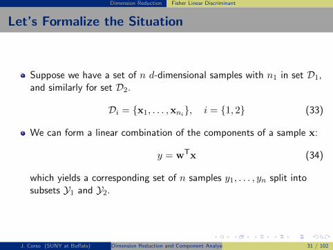
Let’s Formalize the Situation
Suppose we have a set of n d-dimensional samples with n1 in set D1,and similarly for set D2.
Di = {x1, . . . ,xni}, i = {1, 2} (33)
We can form a linear combination of the components of a sample x:
y = wTx (34)
which yields a corresponding set of n samples y1, . . . , yn split intosubsets Y1 and Y2.
J. Corso (SUNY at Buffalo) Dimension Reduction and Component Analysis 31 / 102
Dimension Reduction Fisher Linear Discriminant
Let’s Formalize the Situation
Suppose we have a set of n d-dimensional samples with n1 in set D1,and similarly for set D2.
Di = {x1, . . . ,xni}, i = {1, 2} (33)
We can form a linear combination of the components of a sample x:
y = wTx (34)
which yields a corresponding set of n samples y1, . . . , yn split intosubsets Y1 and Y2.
J. Corso (SUNY at Buffalo) Dimension Reduction and Component Analysis 31 / 102

Dimension Reduction Fisher Linear Discriminant
Geometrically, This is a Projection
If we constrain the norm of w to be 1 (i.e., ‖w‖ = 1) then we canconceptualize that each yi is the projection of the corresponding xionto a line in the direction of w.
0.5 1 1.5
0.5
1
1.5
2
0.5 1 1.5x1
-0.5
0.5
1
1.5
2
x2
w
w
x1
x2
FIGURE 3.5. Projection of the same set of samples onto two different lines in the di-rections marked w. The figure on the right shows greater separation between the redand black projected points. From: Richard O. Duda, Peter E. Hart, and David G. Stork,Pattern Classification. Copyright c© 2001 by John Wiley & Sons, Inc.
Does the magnitude of w have any real significance?
J. Corso (SUNY at Buffalo) Dimension Reduction and Component Analysis 32 / 102

Dimension Reduction Fisher Linear Discriminant
What is a Good Projection?
For our two-class setup, it should be clear that we want the projectionthat will have those samples from class ω1 falling into one cluster (onthe line) and those samples from class ω2 falling into a separatecluster (on the line).
However, this may not be possible depending on our underlyingclasses.
So, how do we find the best direction w?
J. Corso (SUNY at Buffalo) Dimension Reduction and Component Analysis 33 / 102

Dimension Reduction Fisher Linear Discriminant
Separation of the Projected Means
Let mi be the d-dimensional sample mean for class i:
mi =1
ni
∑
x∈Di
x . (35)
Then the sample mean for the projected points is
m̃i =1
ni
∑
y∈Yiy (36)
=1
ni
∑
x∈Di
wTx (37)
= wTmi . (38)
And, thus, is simply the projection of mi.
J. Corso (SUNY at Buffalo) Dimension Reduction and Component Analysis 34 / 102

Dimension Reduction Fisher Linear Discriminant
Distance Between Projected Means
The distance between projected means is thus
|m̃1 − m̃2| = |wT (m1 −m2)| (39)
The scale of w: we can make this distance arbitrarily large by scalingw.
Rather, we want to make this distance large relative to some measureof the standard deviation. ...This story we’ve heard before.
J. Corso (SUNY at Buffalo) Dimension Reduction and Component Analysis 35 / 102

Dimension Reduction Fisher Linear Discriminant
The Scatter
To capture this variation, we compute the scatter
s̃2i =∑
y∈Yi(y − m̃i)
2 (40)
which is essentially a scaled sampled variance.
From this, we can estimate the variance of the pooled data:
1
n
(s̃21 + s̃22
). (41)
s̃21 + s̃22 is called the total within-class scatter of the projectedsamples.
J. Corso (SUNY at Buffalo) Dimension Reduction and Component Analysis 36 / 102

Dimension Reduction Fisher Linear Discriminant
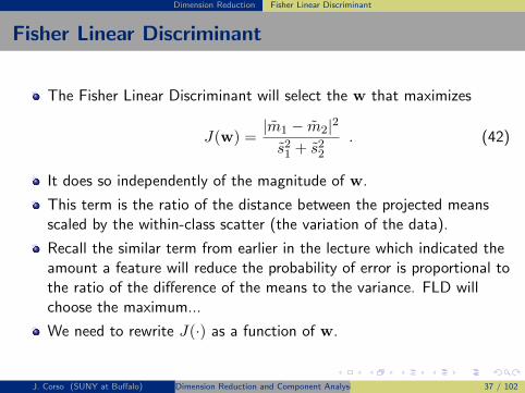
Fisher Linear Discriminant
The Fisher Linear Discriminant will select the w that maximizes
J(w) =|m̃1 − m̃2|2
s̃21 + s̃22. (42)
It does so independently of the magnitude of w.
This term is the ratio of the distance between the projected meansscaled by the within-class scatter (the variation of the data).
Recall the similar term from earlier in the lecture which indicated theamount a feature will reduce the probability of error is proportional tothe ratio of the difference of the means to the variance. FLD willchoose the maximum...
We need to rewrite J(·) as a function of w.
J. Corso (SUNY at Buffalo) Dimension Reduction and Component Analysis 37 / 102

Dimension Reduction Fisher Linear Discriminant
Fisher Linear Discriminant
The Fisher Linear Discriminant will select the w that maximizes
J(w) =|m̃1 − m̃2|2
s̃21 + s̃22. (42)
It does so independently of the magnitude of w.
This term is the ratio of the distance between the projected meansscaled by the within-class scatter (the variation of the data).
Recall the similar term from earlier in the lecture which indicated theamount a feature will reduce the probability of error is proportional tothe ratio of the difference of the means to the variance. FLD willchoose the maximum...
We need to rewrite J(·) as a function of w.
J. Corso (SUNY at Buffalo) Dimension Reduction and Component Analysis 37 / 102
Dimension Reduction Fisher Linear Discriminant
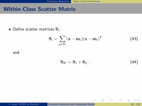
Within-Class Scatter Matrix
Define scatter matrices Si:
Si =∑
x∈Di
(x−mi)(x−mi)T (43)
and
SW = S1 + S2 . (44)
SW is called the within-class scatter matrix.
SW is symmetric and positive semidefinite.
In typical cases, when is SW nonsingular?
J. Corso (SUNY at Buffalo) Dimension Reduction and Component Analysis 38 / 102

Dimension Reduction Fisher Linear Discriminant
Within-Class Scatter Matrix
Deriving the sum of scatters.
s̃2i =∑
x∈Di
(wTx−wTmi
)2(45)
=∑
x∈Di
wT (x−mi) (x−mi)T w (46)
= wTSiw (47)
We can therefore write the sum of the scatters as an explicit functionof w:
s̃21 + s̃22 = wTSWw (48)
J. Corso (SUNY at Buffalo) Dimension Reduction and Component Analysis 39 / 102

Dimension Reduction Fisher Linear Discriminant
Between-Class Scatter Matrix
The separation of the projected means obeys
(m̃1 − m̃2)2 =
(wTm1 −wTm2
)2(49)
= wT (m1 −m2) (m1 −m2)T w (50)
= wTSBw (51)
Here, SB is called the between-class scatter matrix:
SB = (m1 −m2) (m1 −m2)T (52)
SB is also symmetric and positive semidefinite.
When is SB nonsingular?
J. Corso (SUNY at Buffalo) Dimension Reduction and Component Analysis 40 / 102

Dimension Reduction Fisher Linear Discriminant
Rewriting the FLD J(·)
We can rewrite our objective as a function of w.
J(w) =wTSBw
wTSWw(53)
This is the generalized Rayleigh quotient.
The vector w that maximizes J(·) must satisfy
SBw = λSWw (54)
which is a generalized eigenvalue problem.
For nonsingular SW (typical), we can write this as a standardeigenvalue problem:
S−1W SBw = λw (55)
J. Corso (SUNY at Buffalo) Dimension Reduction and Component Analysis 41 / 102
Dimension Reduction Fisher Linear Discriminant
Simplifying
Since ‖w‖ is not important and SBw is always in the direction of(m1 −m2), we can simplify
w∗ = S−1W (m1 −m2) (56)
w∗ maximizes J(·) and is the Fisher Linear Discriminant.
The FLD converts a many-dimensional problem to a one-dimensionalone.
One still must find the threshold. This is easy for known densities,but not so easy in general.
J. Corso (SUNY at Buffalo) Dimension Reduction and Component Analysis 42 / 102

Comparisons Classic
A Classic PCA vs. FLD comparisonSource: Belhumeur et al. IEEE TPAMI 19(7) 711–720. 1997.
PCA maximizes the totalscatter across all classes.
PCA projections are thusoptimal for reconstructionfrom a low dimensionalbasis, but not necessarilyfrom a discriminationstandpoint.
FLD maximizes the ratio ofthe between-class scatterand the within-class scatter.
FLD tries to “shape” thescatter to make it moreeffective for classification.
714 IEEE TRANSACTIONS ON PATTERN ANALYSIS AND MACHINE INTELLIGENCE, VOL. 19, NO. 7, JULY 1997
classification. This method selects W in [1] in such a waythat the ratio of the between-class scatter and the within-class scatter is maximized.
Let the between-class scatter matrix be defined as
S NB i ii
c
iT
= - -=Â m m m mc hc h
1
and the within-class scatter matrix be defined as
SW k iX
k iT
i
c
k i
= - -Œ= x x
x
m mc hc h1
where m i is the mean image of class Xi , and Ni is the num-ber of samples in class Xi . If SW is nonsingular, the optimalprojection Wopt is chosen as the matrix with orthonormal
columns which maximizes the ratio of the determinant ofthe between-class scatter matrix of the projected samples tothe determinant of the within-class scatter matrix of theprojected samples, i.e.,
WW S W
W S Wopt W
TB
TW
m
=
=
arg max
w w w1 2 K (4)
where wi i m= 1 2, , ,Kn s is the set of generalized eigen-
vectors of SB and SW corresponding to the m largest gener-
alized eigenvalues l i i m= 1 2, , ,Kn s, i.e.,
S S i mB i i W iw w= =l , , , ,1 2 K
Note that there are at most c - 1 nonzero generalized eigen-values, and so an upper bound on m is c - 1, where c is thenumber of classes. See [4].
To illustrate the benefits of class specific linear projec-tion, we constructed a low dimensional analogue to theclassification problem in which the samples from each classlie near a linear subspace. Fig. 2 is a comparison of PCAand FLD for a two-class problem in which the samples fromeach class are randomly perturbed in a direction perpen-dicular to a linear subspace. For this example, N = 20, n = 2,and m = 1. So, the samples from each class lie near a linepassing through the origin in the 2D feature space. BothPCA and FLD have been used to project the points from 2Ddown to 1D. Comparing the two projections in the figure,PCA actually smears the classes together so that they are nolonger linearly separable in the projected space. It is clearthat, although PCA achieves larger total scatter, FLDachieves greater between-class scatter, and, consequently,classification is simplified.
In the face recognition problem, one is confronted withthe difficulty that the within-class scatter matrix SW
n nŒ ¥R
is always singular. This stems from the fact that the rank ofSW is at most N - c, and, in general, the number of imagesin the learning set N is much smaller than the number ofpixels in each image n. This means that it is possible tochoose the matrix W such that the within-class scatter of theprojected samples can be made exactly zero.
In order to overcome the complication of a singular SW ,we propose an alternative to the criterion in (4). This
method, which we call Fisherfaces, avoids this problem byprojecting the image set to a lower dimensional space sothat the resulting within-class scatter matrix SW is nonsin-gular. This is achieved by using PCA to reduce the dimen-sion of the feature space to N - c, and then applying thestandard FLD defined by (4) to reduce the dimension to c - 1.More formally, Wopt is given by
W W WoptT
fldT
pcaT= (5)
where
W W S W
WW W S W W
W W S W W
pca W
TT
fld W
TpcaT
B pca
TpcaT
W pca
=
=
arg max
arg max
Note that the optimization for Wpca is performed over
n ¥ (N - c) matrices with orthonormal columns, while theoptimization for Wfld is performed over (N - c) ¥ m matrices
with orthonormal columns. In computing Wpca , we have
thrown away only the smallest c - 1 principal components.There are certainly other ways of reducing the within-
class scatter while preserving between-class scatter. Forexample, a second method which we are currently investi-gating chooses W to maximize the between-class scatter ofthe projected samples after having first reduced the within-class scatter. Taken to an extreme, we can maximize thebetween-class scatter of the projected samples subject to theconstraint that the within-class scatter is zero, i.e.,
W W S Wopt W
TB=
Œarg max
:
(6)
where : is the set of n ¥ m matrices with orthonormal col-umns contained in the kernel of SW .
Fig. 2. A comparison of principal component analysis (PCA) andFisher’s linear discriminant (FLD) for a two class problem where datafor each class lies near a linear subspace.
J. Corso (SUNY at Buffalo) Dimension Reduction and Component Analysis 43 / 102

Comparisons Case Study: Faces
Case Study: EigenFaces versus FisherFacesSource: Belhumeur et al. IEEE TPAMI 19(7) 711–720. 1997.
Analysis of classic pattern recognition techniques (PCA and FLD) todo face recognition.
Fixed pose but varying illumination.
The variation in the resulting images caused by the varyingillumination will nearly always dominate the variation caused by anidentity change.
IEEE TRANSACTIONS ON PATTERN ANALYSIS AND MACHINE INTELLIGENCE, VOL. 19, NO. 7, JULY 1997 711
Eigenfaces vs. Fisherfaces: RecognitionUsing Class Specific Linear Projection
Peter N. Belhumeur, Joao~ P. Hespanha, and David J. Kriegman
Abstract —We develop a face recognition algorithm which is insensitive to large variation in lighting direction and facial expression.Taking a pattern classification approach, we consider each pixel in an image as a coordinate in a high-dimensional space. We takeadvantage of the observation that the images of a particular face, under varying illumination but fixed pose, lie in a 3D linearsubspace of the high dimensional image space—if the face is a Lambertian surface without shadowing. However, since faces arenot truly Lambertian surfaces and do indeed produce self-shadowing, images will deviate from this linear subspace. Rather thanexplicitly modeling this deviation, we linearly project the image into a subspace in a manner which discounts those regions of theface with large deviation. Our projection method is based on Fisher’s Linear Discriminant and produces well separated classes in alow-dimensional subspace, even under severe variation in lighting and facial expressions. The Eigenface technique, another methodbased on linearly projecting the image space to a low dimensional subspace, has similar computational requirements. Yet, extensiveexperimental results demonstrate that the proposed “Fisherface” method has error rates that are lower than those of the Eigenfacetechnique for tests on the Harvard and Yale Face Databases.
Index Terms —Appearance-based vision, face recognition, illumination invariance, Fisher’s linear discriminant.
—————————— ✦ ——————————
1 INTRODUCTION
Within the last several years, numerous algorithms havebeen proposed for face recognition; for detailed surveys see[1], [2]. While much progress has been made toward recog-nizing faces under small variations in lighting, facial ex-pression and pose, reliable techniques for recognition undermore extreme variations have proven elusive.
In this paper, we outline a new approach for face recogni-tion—one that is insensitive to large variations in lightingand facial expressions. Note that lighting variability includesnot only intensity, but also direction and number of lightsources. As is evident from Fig. 1, the same person, with thesame facial expression, and seen from the same viewpoint,can appear dramatically different when light sources illumi-nate the face from different directions. See also Fig. 4.
Our approach to face recognition exploits two observations:
1) All of the images of a Lambertian surface, taken froma fixed viewpoint, but under varying illumination, liein a 3D linear subspace of the high-dimensional imagespace [3].
2) Because of regions of shadowing, specularities, andfacial expressions, the above observation does not ex-actly hold. In practice, certain regions of the face mayhave variability from image to image that often devi-ates significantly from the linear subspace, and, con-sequently, are less reliable for recognition.
We make use of these observations by finding a linearprojection of the faces from the high-dimensional image
space to a significantly lower dimensional feature spacewhich is insensitive both to variation in lighting directionand facial expression. We choose projection directions thatare nearly orthogonal to the within-class scatter, projectingaway variations in lighting and facial expression whilemaintaining discriminability. Our method Fisherfaces, aderivative of Fisher’s Linear Discriminant (FLD) [4], [5],maximizes the ratio of between-class scatter to that ofwithin-class scatter.
The Eigenface method is also based on linearly project-ing the image space to a low dimensional feature space [6],[7], [8]. However, the Eigenface method, which uses princi-pal components analysis (PCA) for dimensionality reduc-tion, yields projection directions that maximize the totalscatter across all classes, i.e., across all images of all faces. Inchoosing the projection which maximizes total scatter, PCAretains unwanted variations due to lighting and facialexpression. As illustrated in Figs. 1 and 4 and stated byMoses et al., “the variations between the images of the sameface due to illumination and viewing direction are almostalways larger than image variations due to change in faceidentity” [9]. Thus, while the PCA projections are optimal
0162-8828/97/$10.00 © 1997 IEEE
————————————————
• The authors are with the Center for Computational Vision and Control, Dept.of Electrical Engineering, Yale University, New Haven, CT 06520-8267.E-mail: {belhumeur, kriegman}@yale.edu, [email protected].
Manuscript received 15 Feb. 1996 revised 20 Mar. 1997. Recommended for accep-tance by J. Daugman.For information on obtaining reprints of this article, please send e-mail to:[email protected], and reference IEEECS Log Number 104797.
Fig. 1. The same person seen under different lighting conditions canappear dramatically different: In the left image, the dominant lightsource is nearly head-on; in the right image, the dominant light sourceis from above and to the right.
J. Corso (SUNY at Buffalo) Dimension Reduction and Component Analysis 44 / 102

Comparisons Case Study: Faces
Case Study: EigenFaces versus FisherFacesSource: Belhumeur et al. IEEE TPAMI 19(7) 711–720. 1997.
BELHUMEUR ET AL.: EIGENFACES VS. FISHERFACES: RECOGNITION USING CLASS SPECIFIC LINEAR PROJECTION 717
image, the glasses were removed. If the person normallywore glasses, those were used; if not, a random pair was bor-rowed. Images 3-5 were acquired by illuminating the face ina neutral expression with a Luxolamp in three positions. Thelast five images were acquired under ambient lighting withdifferent expressions (happy, sad, winking, sleepy, and sur-prised). For the Eigenface and correlation tests, the imageswere normalized to have zero mean and unit variance, as thisimproved the performance of these methods. The imageswere manually centered and cropped to two different scales:The larger images included the full face and part of the back-ground while the closely cropped ones included internalstructures such as the brow, eyes, nose, mouth, and chin, butdid not extend to the occluding contour.
In this test, error rates were determined by the “leaving-one-out” strategy [4]: To classify an image of a person, thatimage was removed from the data set and the dimension-ality reduction matrix W was computed. All images in thedatabase, excluding the test image, were then projecteddown into the reduced space to be used for classification.Recognition was performed using a nearest neighbor classi-fier. Note that for this test, each person in the learning set isrepresented by the projection of ten images, except for thetest person who is represented by only nine.
In general, the performance of the Eigenface methodvaries with the number of principal components. Thus, be-fore comparing the Linear Subspace and Fisherface methodswith the Eigenface method, we first performed an experi-
Interpolating between Subsets 1 and 5Method Reduced Error Rate (%)
Space Subset 2 Subset 3 Subset 4Eigenface 4 53.3 75.4 52.9
10 11.11 33.9 20.0Eigenface 4 31.11 60.0 29.4w/o 1st 3 10 6.7 20.0 12.9
Correlation 129 0.0 21.54 7.1Linear Subspace 15 0.0 1.5 0.0
Fisherface 4 0.0 0.0 1.2
Fig. 6. Interpolation: When each of the methods is trained on images from both near frontal and extreme lighting (Subsets 1 and 5), the graph andcorresponding table show the relative performance under intermediate lighting conditions.
Fig. 7. The Yale database contains 160 frontal face images covering 16 individuals taken under 10 different conditions: A normal image underambient lighting, one with or without glasses, three images taken with different point light sources, and five different facial expressions.
J. Corso (SUNY at Buffalo) Dimension Reduction and Component Analysis 45 / 102

Comparisons Case Study: Faces
Is Linear Okay For Faces?Source: Belhumeur et al. IEEE TPAMI 19(7) 711–720. 1997.
Fact: all of the images of a Lambertian surface, taken from a fixedviewpoint, but under varying illumination, lie in a 3D linear subspaceof the high-dimensional image space.
But, in the presence of shadowing, specularities, and facialexpressions, the above statement will not hold. This will ultimatelyresult in deviations from the 3D linear subspace and worseclassification accuracy.
J. Corso (SUNY at Buffalo) Dimension Reduction and Component Analysis 46 / 102

Comparisons Case Study: Faces
Method 1: CorrelationSource: Belhumeur et al. IEEE TPAMI 19(7) 711–720. 1997.
Consider a set of N training images, {x1,x2, . . . ,xN}.We know that each of the N images belongs to one of c classes andcan define a C(·) function to map the image x into a class ωc.
Pre-Processing – each image is normalized to have zero mean andunit variance.
Why?
Gets rid of the light source intensity and the effects of a camera’sautomatic gain control.
For a query image x, we select the class of the training image that isthe nearest neighbor in the image space:
x∗ = argmin{xi}‖x− xi‖ then decide C(x∗) (57)
where we have vectorized each image.
J. Corso (SUNY at Buffalo) Dimension Reduction and Component Analysis 47 / 102
Comparisons Case Study: Faces
Method 1: CorrelationSource: Belhumeur et al. IEEE TPAMI 19(7) 711–720. 1997.
What are the advantages and disadvantages of the correlation basedmethod in this context?
Computationally expensive.
Require large amount of storage.
Noise may play a role.
Highly parallelizable.
J. Corso (SUNY at Buffalo) Dimension Reduction and Component Analysis 48 / 102
Comparisons Case Study: Faces
Method 2: EigenFacesSource: Belhumeur et al. IEEE TPAMI 19(7) 711–720. 1997. The original paper isTurk and Pentland, “Eigenfaces for Recognition” Journal of CognitiveNeuroscience, 3(1). 1991.
Quickly recall the main idea of PCA.
Define a linear projection of the original n-d image space into an m-dspace with m < n or m� n, which yields new vectors y:
yk =WTxk k = 1, 2, . . . , N (58)
where W ∈ Rn×m.
Define the total scatter matrix ST as
ST =N∑
k=1
(xk − µ) (xk − µ)T (59)
where µ is the sample mean image.
J. Corso (SUNY at Buffalo) Dimension Reduction and Component Analysis 49 / 102

Comparisons Case Study: Faces
Method 2: EigenFacesSource: Belhumeur et al. IEEE TPAMI 19(7) 711–720. 1997. The original paper isTurk and Pentland, “Eigenfaces for Recognition” Journal of CognitiveNeuroscience, 3(1). 1991.
The scatter of the projected vectors {y1,y2, . . . ,yN} is
WTSTW (60)
Wopt is chosen to maximize the determinant of the total scattermatrix of the projected vectors:
Wopt = argmaxW|WTSTW | (61)
=[w1 w2 . . . wm
](62)
where {wi|i = 1, d, . . . ,m} is the set of n-d eigenvectors of STcorresponding to the largest m eigenvalues.
J. Corso (SUNY at Buffalo) Dimension Reduction and Component Analysis 50 / 102
Comparisons Case Study: Faces
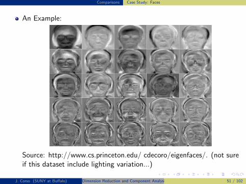
An Example:
Source: http://www.cs.princeton.edu/ cdecoro/eigenfaces/. (not sureif this dataset include lighting variation...)
J. Corso (SUNY at Buffalo) Dimension Reduction and Component Analysis 51 / 102

Comparisons Case Study: Faces
Method 2: EigenFacesSource: Belhumeur et al. IEEE TPAMI 19(7) 711–720. 1997. The original paper isTurk and Pentland, “Eigenfaces for Recognition” Journal of CognitiveNeuroscience, 3(1). 1991.
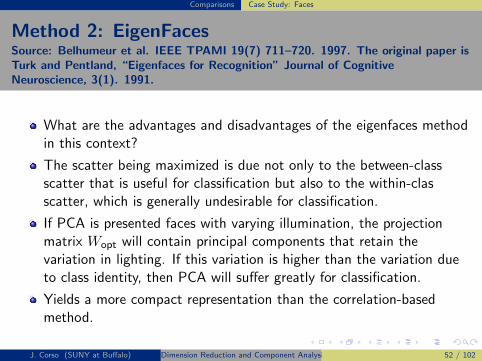
What are the advantages and disadvantages of the eigenfaces methodin this context?
The scatter being maximized is due not only to the between-classscatter that is useful for classification but also to the within-classcatter, which is generally undesirable for classification.
If PCA is presented faces with varying illumination, the projectionmatrix Wopt will contain principal components that retain thevariation in lighting. If this variation is higher than the variation dueto class identity, then PCA will suffer greatly for classification.
Yields a more compact representation than the correlation-basedmethod.
J. Corso (SUNY at Buffalo) Dimension Reduction and Component Analysis 52 / 102
Comparisons Case Study: Faces
Method 2: EigenFacesSource: Belhumeur et al. IEEE TPAMI 19(7) 711–720. 1997. The original paper isTurk and Pentland, “Eigenfaces for Recognition” Journal of CognitiveNeuroscience, 3(1). 1991.
What are the advantages and disadvantages of the eigenfaces methodin this context?
The scatter being maximized is due not only to the between-classscatter that is useful for classification but also to the within-classcatter, which is generally undesirable for classification.
If PCA is presented faces with varying illumination, the projectionmatrix Wopt will contain principal components that retain thevariation in lighting. If this variation is higher than the variation dueto class identity, then PCA will suffer greatly for classification.
Yields a more compact representation than the correlation-basedmethod.
J. Corso (SUNY at Buffalo) Dimension Reduction and Component Analysis 52 / 102

Comparisons Case Study: Faces
Method 3: Linear SubspacesSource: Belhumeur et al. IEEE TPAMI 19(7) 711–720. 1997.
Use Lambertian model directly.
Consider a point p on a Lambertian surface illuminated by a pointlight source at infinity.
Let s ∈ R3 signify the product of the light source intensity with theunit vector for the light source direction.
The image intensity of the surface at p when viewed by a camera is
E(p) = a(p)n(p)Ts (63)
where n(p) is the unit inward normal vector to the surface at point p,and a(p) is the albedo of the surface at p (a scalar).
Hence, the image intensity of the point p is linear on s.
J. Corso (SUNY at Buffalo) Dimension Reduction and Component Analysis 53 / 102

Comparisons Case Study: Faces
Method 3: Linear SubspacesSource: Belhumeur et al. IEEE TPAMI 19(7) 711–720. 1997.
So, if we assume no shadowing, given three images of a Lambertiansurface from the same viewpoint under three known, linearlyindependent light source directions, the albedo and surface normalcan be recovered.
Alternatively, one can reconstruct the image of the surface under anarbitrary lighting direction by a linear combination of the threeoriginal images.
This fact can be used for classification.
For each face (class) use three or more images taken under differentlighting conditions to construct a 3D basis for the linear subspace.
For recognition, compute the distance of a new image to each linearsubspace and choose the face corresponding to the shortest distance.
J. Corso (SUNY at Buffalo) Dimension Reduction and Component Analysis 54 / 102

Comparisons Case Study: Faces
Method 3: Linear SubspacesSource: Belhumeur et al. IEEE TPAMI 19(7) 711–720. 1997.
Pros and Cons?
If there is no noise or shadowing, this method will achieve error freeclassification under any lighting conditions (and if the surface isindeed Lambertian).
Faces inevitably have self-shadowing.
Faces have expressions...
Still pretty computationally expensive (linear in number of classes).
J. Corso (SUNY at Buffalo) Dimension Reduction and Component Analysis 55 / 102
Comparisons Case Study: Faces
Method 4: FisherFacesSource: Belhumeur et al. IEEE TPAMI 19(7) 711–720. 1997.
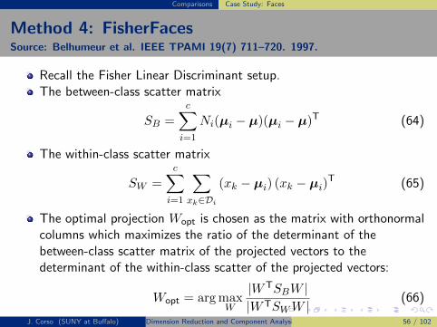
Recall the Fisher Linear Discriminant setup.The between-class scatter matrix
SB =
c∑
i=1
Ni(µi − µ)(µi − µ)T (64)
The within-class scatter matrix
SW =
c∑
i=1
∑
xk∈Di
(xk − µi) (xk − µi)T (65)
The optimal projection Wopt is chosen as the matrix with orthonormalcolumns which maximizes the ratio of the determinant of thebetween-class scatter matrix of the projected vectors to thedeterminant of the within-class scatter of the projected vectors:
Wopt = argmaxW
|WTSBW ||WTSWW |
(66)
J. Corso (SUNY at Buffalo) Dimension Reduction and Component Analysis 56 / 102

Comparisons Case Study: Faces
Method 4: FisherFacesSource: Belhumeur et al. IEEE TPAMI 19(7) 711–720. 1997.
The eigenvectors {wi|i = 1, 2, . . . ,m} corresponding to the m largesteigenvalues of the following generalized eigenvalue problem compriseWopt:
SBwi = λiSWwi, i = 1, 2, . . . ,m (67)
This is a multi-class version of the FLD, which we will discuss in moredetail.
In face recognition, things get a little more complicated because thewithin-class scatter matrix SW is always singular.
This is because the rank of SW is at most N − c and the number ofimages in the learning set are commonly much smaller than thenumber of pixels in the image.
This means we can choose W such that the within-class scatter isexactly zero.
J. Corso (SUNY at Buffalo) Dimension Reduction and Component Analysis 57 / 102

Comparisons Case Study: Faces
Method 4: FisherFacesSource: Belhumeur et al. IEEE TPAMI 19(7) 711–720. 1997.
To overcome this, project the image set to a lower dimensional spaceso that the resulting within-class scatter matrix SW is nonsingular.
How?
PCA to first reduce the dimension to N − c and the FLD to reduce itto c− 1.
WTopt is given by the product WT
FLDWTPCA where
WPCA = argmaxW|WTSTW | (68)
WFLD = argmaxW
|WTWTPCASBWPCAW |
|WTWTPCASWWPCAW |
(69)
J. Corso (SUNY at Buffalo) Dimension Reduction and Component Analysis 58 / 102

Comparisons Case Study: Faces
Experiment 1 and 2: Variation in LightingSource: Belhumeur et al. IEEE TPAMI 19(7) 711–720. 1997.
Hypothesis: face recognition algorithms will perform better if theyexploit the fact that images of a Lambertian surface lie in a linearsubspace.
Used Hallinan’s Harvard Database which sampled the space of lightsource directions in 15 degree incremements.
Used 330 images of five people (66 of each) and extracted fivesubsets.
Classification is nearest neighbor in all cases.
J. Corso (SUNY at Buffalo) Dimension Reduction and Component Analysis 59 / 102

Comparisons Case Study: Faces
Experiment 1 and 2: Variation in LightingSource: Belhumeur et al. IEEE TPAMI 19(7) 711–720. 1997.
BELHUMEUR ET AL.: EIGENFACES VS. FISHERFACES: RECOGNITION USING CLASS SPECIFIC LINEAR PROJECTION 715
3 EXPERIMENTAL RESULTS
In this section, we present and discuss each of the afore-mentioned face recognition techniques using two differentdatabases. Because of the specific hypotheses that wewanted to test about the relative performance of the consid-ered algorithms, many of the standard databases were in-appropriate. So, we have used a database from the HarvardRobotics Laboratory in which lighting has been systemati-cally varied. Secondly, we have constructed a database atYale that includes variation in both facial expression andlighting. 1
3.1 Variation in LightingThe first experiment was designed to test the hypothesisthat under variable illumination, face recognition algo-rithms will perform better if they exploit the fact that im-ages of a Lambertian surface lie in a linear subspace. Morespecifically, the recognition error rates for all four algo-rithms described in Section 2 are compared using an im-age database constructed by Hallinan at the Harvard Ro-botics Laboratory [14], [15]. In each image in this data-base, a subject held his/her head steady while being illu-minated by a dominant light source. The space of lightsource directions, which can be parameterized by spheri-cal angles, was then sampled in 15$ increments. See Fig. 3.From this database, we used 330 images of five people (66of each). We extracted five subsets to quantify the effectsof varying lighting. Sample images from each subset areshown in Fig. 4.
Subset 1 contains 30 images for which both the longitudi-nal and latitudinal angles of light source direction arewithin 15$ of the camera axis, including the lighting
1. The Yale database is available for download from http://cvc.yale.edu.
direction coincident with the camera’s optical axis.Subset 2 contains 45 images for which the greater of the
longitudinal and latitudinal angles of light source di-rection are 30$ from the camera axis.
Subset 3 contains 65 images for which the greater of thelongitudinal and latitudinal angles of light source di-rection are 45$ from the camera axis.
Subset 4 contains 85 images for which the greater of thelongitudinal and latitudinal angles of light source di-rection are 60$ from the camera axis.
Subset 5 contains 105 images for which the greater of thelongitudinal and latitudinal angles of light source di-rection are 75$ from the camera axis.
For all experiments, classification was performed using anearest neighbor classifier. All training images of an indi-
Fig. 3. The highlighted lines of longitude and latitude indicate the lightsource directions for Subsets 1 through 5. Each intersection of a lon-gitudinal and latitudinal line on the right side of the illustration has acorresponding image in the database.
Fig. 4. Example images from each subset of the Harvard Database used to test the four algorithms.
J. Corso (SUNY at Buffalo) Dimension Reduction and Component Analysis 60 / 102

Comparisons Case Study: Faces
Experiment 1: Variation in LightingSource: Belhumeur et al. IEEE TPAMI 19(7) 711–720. 1997.
BELHUMEUR ET AL.: EIGENFACES VS. FISHERFACES: RECOGNITION USING CLASS SPECIFIC LINEAR PROJECTION 715
3 EXPERIMENTAL RESULTS
In this section, we present and discuss each of the afore-mentioned face recognition techniques using two differentdatabases. Because of the specific hypotheses that wewanted to test about the relative performance of the consid-ered algorithms, many of the standard databases were in-appropriate. So, we have used a database from the HarvardRobotics Laboratory in which lighting has been systemati-cally varied. Secondly, we have constructed a database atYale that includes variation in both facial expression andlighting. 1
3.1 Variation in LightingThe first experiment was designed to test the hypothesisthat under variable illumination, face recognition algo-rithms will perform better if they exploit the fact that im-ages of a Lambertian surface lie in a linear subspace. Morespecifically, the recognition error rates for all four algo-rithms described in Section 2 are compared using an im-age database constructed by Hallinan at the Harvard Ro-botics Laboratory [14], [15]. In each image in this data-base, a subject held his/her head steady while being illu-minated by a dominant light source. The space of lightsource directions, which can be parameterized by spheri-cal angles, was then sampled in 15$ increments. See Fig. 3.From this database, we used 330 images of five people (66of each). We extracted five subsets to quantify the effectsof varying lighting. Sample images from each subset areshown in Fig. 4.
Subset 1 contains 30 images for which both the longitudi-nal and latitudinal angles of light source direction arewithin 15$ of the camera axis, including the lighting
1. The Yale database is available for download from http://cvc.yale.edu.
direction coincident with the camera’s optical axis.Subset 2 contains 45 images for which the greater of the
longitudinal and latitudinal angles of light source di-rection are 30$ from the camera axis.
Subset 3 contains 65 images for which the greater of thelongitudinal and latitudinal angles of light source di-rection are 45$ from the camera axis.
Subset 4 contains 85 images for which the greater of thelongitudinal and latitudinal angles of light source di-rection are 60$ from the camera axis.
Subset 5 contains 105 images for which the greater of thelongitudinal and latitudinal angles of light source di-rection are 75$ from the camera axis.
For all experiments, classification was performed using anearest neighbor classifier. All training images of an indi-
Fig. 3. The highlighted lines of longitude and latitude indicate the lightsource directions for Subsets 1 through 5. Each intersection of a lon-gitudinal and latitudinal line on the right side of the illustration has acorresponding image in the database.
Fig. 4. Example images from each subset of the Harvard Database used to test the four algorithms.J. Corso (SUNY at Buffalo) Dimension Reduction and Component Analysis 61 / 102

Comparisons Case Study: Faces
Experiment 1: Variation in Lighting – ExtrapolationSource: Belhumeur et al. IEEE TPAMI 19(7) 711–720. 1997.
Train on Subset 1.
Test of Subsets 1,2,and 3.716 IEEE TRANSACTIONS ON PATTERN ANALYSIS AND MACHINE INTELLIGENCE, VOL. 19, NO. 7, JULY 1997
vidual were projected into the feature space. The imageswere cropped within the face so that the contour of thehead was excluded.2 For the Eigenface and correlation tests,the images were normalized to have zero mean and unitvariance, as this improved the performance of these meth-ods. For the Eigenface method, results are shown when tenprincipal components were used. Since it has been sug-gested that the first three principal components are primar-ily due to lighting variation and that recognition rates canbe improved by eliminating them, error rates are also pre-sented using principal components four through thirteen.
We performed two experiments on the Harvard Data-base: extrapolation and interpolation. In the extrapolationexperiment, each method was trained on samples fromSubset 1 and then tested using samples from Subsets 1, 2,and 3.3 Since there are 30 images in the training set, cor-relation is equivalent to the Eigenface method using 29principal components. Fig. 5 shows the result from thisexperiment.
In the interpolation experiment, each method was trainedon Subsets 1 and 5 and then tested the methods on Subsets 2,3, and 4. Fig. 6 shows the result from this experiment.
These two experiments reveal a number of interestingpoints:
1) All of the algorithms perform perfectly when lightingis nearly frontal. However, as lighting is moved off
2. We have observed that the error rates are reduced for all methods whenthe contour is included and the subject is in front of a uniform background.However, all methods performed worse when the background varies.
3. To test the methods with an image from Subset 1, that image was removedfrom the training set, i.e., we employed the “leaving-one-out” strategy [4].
axis, there is a significant performance differencebetween the two class-specific methods and the Ei-genface method.
2) It has also been noted that the Eigenface method isequivalent to correlation when the number of Eigen-faces equals the size of the training set [17], and sinceperformance increases with the dimension of the ei-genspace, the Eigenface method should do no betterthan correlation [26]. This is empirically demonstratedas well.
3) In the Eigenface method, removing the first threeprincipal components results in better performanceunder variable lighting conditions.
4) While the Linear Subspace method has error rates thatare competitive with the Fisherface method, it re-quires storing more than three times as much infor-mation and takes three times as long.
5) The Fisherface method had error rates lower than theEigenface method and required less computation time.
3.2 Variation in Facial Expression, Eye Wear, andLighting
Using a second database constructed at the Yale Center forComputational Vision and Control, we designed tests to de-termine how the methods compared under a different rangeof conditions. For sixteen subjects, ten images were acquiredduring one session in front of a simple background. Subjectsincluded females and males (some with facial hair), andsome wore glasses. Fig. 7 shows ten images of one subject.The first image was taken under ambient lighting in a neutralfacial expression and the person wore glasses. In the second
Extrapolating from Subset 1Method Reduced Error Rate (%)
Space Subset 1 Subset 2 Subset 3Eigenface 4 0.0 31.1 47.7
10 0.0 4.4 41.5Eigenface 4 0.0 13.3 41.5w/o 1st 3 10 0.0 4.4 27.7
Correlation 29 0.0 0.0 33.9Linear Subspace 15 0.0 4.4 9.2
Fisherface 4 0.0 0.0 4.6
Fig. 5. Extrapolation: When each of the methods is trained on images with near frontal illumination (Subset 1), the graph and corresponding table showthe relative performance under extreme light source conditions.
J. Corso (SUNY at Buffalo) Dimension Reduction and Component Analysis 62 / 102
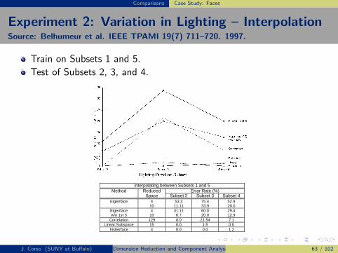
Comparisons Case Study: Faces
Experiment 2: Variation in Lighting – InterpolationSource: Belhumeur et al. IEEE TPAMI 19(7) 711–720. 1997.
Train on Subsets 1 and 5.
Test of Subsets 2, 3, and 4.BELHUMEUR ET AL.: EIGENFACES VS. FISHERFACES: RECOGNITION USING CLASS SPECIFIC LINEAR PROJECTION 717
image, the glasses were removed. If the person normallywore glasses, those were used; if not, a random pair was bor-rowed. Images 3-5 were acquired by illuminating the face ina neutral expression with a Luxolamp in three positions. Thelast five images were acquired under ambient lighting withdifferent expressions (happy, sad, winking, sleepy, and sur-prised). For the Eigenface and correlation tests, the imageswere normalized to have zero mean and unit variance, as thisimproved the performance of these methods. The imageswere manually centered and cropped to two different scales:The larger images included the full face and part of the back-ground while the closely cropped ones included internalstructures such as the brow, eyes, nose, mouth, and chin, butdid not extend to the occluding contour.
In this test, error rates were determined by the “leaving-one-out” strategy [4]: To classify an image of a person, thatimage was removed from the data set and the dimension-ality reduction matrix W was computed. All images in thedatabase, excluding the test image, were then projecteddown into the reduced space to be used for classification.Recognition was performed using a nearest neighbor classi-fier. Note that for this test, each person in the learning set isrepresented by the projection of ten images, except for thetest person who is represented by only nine.
In general, the performance of the Eigenface methodvaries with the number of principal components. Thus, be-fore comparing the Linear Subspace and Fisherface methodswith the Eigenface method, we first performed an experi-
Interpolating between Subsets 1 and 5Method Reduced Error Rate (%)
Space Subset 2 Subset 3 Subset 4Eigenface 4 53.3 75.4 52.9
10 11.11 33.9 20.0Eigenface 4 31.11 60.0 29.4w/o 1st 3 10 6.7 20.0 12.9
Correlation 129 0.0 21.54 7.1Linear Subspace 15 0.0 1.5 0.0
Fisherface 4 0.0 0.0 1.2
Fig. 6. Interpolation: When each of the methods is trained on images from both near frontal and extreme lighting (Subsets 1 and 5), the graph andcorresponding table show the relative performance under intermediate lighting conditions.
Fig. 7. The Yale database contains 160 frontal face images covering 16 individuals taken under 10 different conditions: A normal image underambient lighting, one with or without glasses, three images taken with different point light sources, and five different facial expressions.
J. Corso (SUNY at Buffalo) Dimension Reduction and Component Analysis 63 / 102
Comparisons Case Study: Faces
Experiment 1 and 2: Variation in LightingSource: Belhumeur et al. IEEE TPAMI 19(7) 711–720. 1997.
All of the algorithms perform perfectly when lighting is nearly frontal.However, when lighting is moved off axis, there is significantdifference between the methods (spec. the class-specific methods andthe Eigenface method).
Empirically demonstrated that the Eigenface method is equivalent tocorrelation when the number of Eigenfaces equals the size of thetraining set (Exp. 1).In the Eigenface method, removing the first three principalcomponents results in better performance under variable lightingconditions.Linear Subspace has comparable error rates with the FisherFacemethod, but it requires 3x as much storage and takes three times aslong.The Fisherface method had error rates lower than the Eigenfacemethod and required less computation time.
J. Corso (SUNY at Buffalo) Dimension Reduction and Component Analysis 64 / 102

Comparisons Case Study: Faces
Experiment 1 and 2: Variation in LightingSource: Belhumeur et al. IEEE TPAMI 19(7) 711–720. 1997.
All of the algorithms perform perfectly when lighting is nearly frontal.However, when lighting is moved off axis, there is significantdifference between the methods (spec. the class-specific methods andthe Eigenface method).Empirically demonstrated that the Eigenface method is equivalent tocorrelation when the number of Eigenfaces equals the size of thetraining set (Exp. 1).
In the Eigenface method, removing the first three principalcomponents results in better performance under variable lightingconditions.Linear Subspace has comparable error rates with the FisherFacemethod, but it requires 3x as much storage and takes three times aslong.The Fisherface method had error rates lower than the Eigenfacemethod and required less computation time.
J. Corso (SUNY at Buffalo) Dimension Reduction and Component Analysis 64 / 102

Comparisons Case Study: Faces
Experiment 1 and 2: Variation in LightingSource: Belhumeur et al. IEEE TPAMI 19(7) 711–720. 1997.
All of the algorithms perform perfectly when lighting is nearly frontal.However, when lighting is moved off axis, there is significantdifference between the methods (spec. the class-specific methods andthe Eigenface method).Empirically demonstrated that the Eigenface method is equivalent tocorrelation when the number of Eigenfaces equals the size of thetraining set (Exp. 1).In the Eigenface method, removing the first three principalcomponents results in better performance under variable lightingconditions.
Linear Subspace has comparable error rates with the FisherFacemethod, but it requires 3x as much storage and takes three times aslong.The Fisherface method had error rates lower than the Eigenfacemethod and required less computation time.
J. Corso (SUNY at Buffalo) Dimension Reduction and Component Analysis 64 / 102
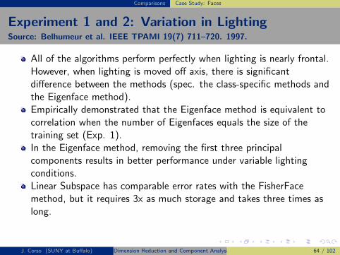
Comparisons Case Study: Faces
Experiment 1 and 2: Variation in LightingSource: Belhumeur et al. IEEE TPAMI 19(7) 711–720. 1997.
All of the algorithms perform perfectly when lighting is nearly frontal.However, when lighting is moved off axis, there is significantdifference between the methods (spec. the class-specific methods andthe Eigenface method).Empirically demonstrated that the Eigenface method is equivalent tocorrelation when the number of Eigenfaces equals the size of thetraining set (Exp. 1).In the Eigenface method, removing the first three principalcomponents results in better performance under variable lightingconditions.Linear Subspace has comparable error rates with the FisherFacemethod, but it requires 3x as much storage and takes three times aslong.
The Fisherface method had error rates lower than the Eigenfacemethod and required less computation time.
J. Corso (SUNY at Buffalo) Dimension Reduction and Component Analysis 64 / 102

Comparisons Case Study: Faces
Experiment 1 and 2: Variation in LightingSource: Belhumeur et al. IEEE TPAMI 19(7) 711–720. 1997.
All of the algorithms perform perfectly when lighting is nearly frontal.However, when lighting is moved off axis, there is significantdifference between the methods (spec. the class-specific methods andthe Eigenface method).Empirically demonstrated that the Eigenface method is equivalent tocorrelation when the number of Eigenfaces equals the size of thetraining set (Exp. 1).In the Eigenface method, removing the first three principalcomponents results in better performance under variable lightingconditions.Linear Subspace has comparable error rates with the FisherFacemethod, but it requires 3x as much storage and takes three times aslong.The Fisherface method had error rates lower than the Eigenfacemethod and required less computation time.
J. Corso (SUNY at Buffalo) Dimension Reduction and Component Analysis 64 / 102
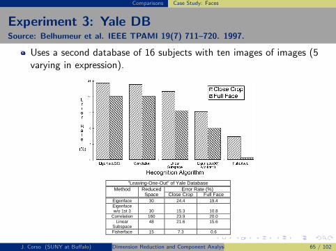
Comparisons Case Study: Faces
Experiment 3: Yale DBSource: Belhumeur et al. IEEE TPAMI 19(7) 711–720. 1997.
Uses a second database of 16 subjects with ten images of images (5varying in expression).
718 IEEE TRANSACTIONS ON PATTERN ANALYSIS AND MACHINE INTELLIGENCE, VOL. 19, NO. 7, JULY 1997
ment to determine the number of principal componentsyielding the lowest error rate. Fig. 8 shows a plot of errorrate vs. the number of principal components, for the closelycropped set, when the initial three principal componentswere retained and when they were dropped.
The relative performance of the algorithms is self evidentin Fig. 9. The Fisherface method had error rates that werebetter than half that of any other method. It seems that theFisherface method chooses the set of projections which per-forms well over a range of lighting variation, facial expres-sion variation, and presence of glasses.
Note that the Linear Subspace method faired compara-tively worse in this experiment than in the lighting experi-ments in the previous section. Because of variation in facialexpression, the images no longer lie in a linear subspace.Since the Fisherface method tends to discount those por-tions of the image that are not significant for recognizing anindividual, the resulting projections W tend to mask theregions of the face that are highly variable. For example, thearea around the mouth is discounted, since it varies quite abit for different facial expressions. On the other hand, thenose, cheeks, and brow are stable over the within-class
Fig. 8. As demonstrated on the Yale Database, the variation in performance of the Eigenface method depends on the number of principal compo-nents retained. Dropping the first three appears to improve performance.
”Leaving-One-Out” of Yale DatabaseMethod Reduced Error Rate (%)
Space Close Crop Full FaceEigenface 30 24.4 19.4Eigenfacew/o 1st 3 30 15.3 10.8
Correlation 160 23.9 20.0Linear
Subspace48 21.6 15.6
Fisherface 15 7.3 0.6
Fig. 9. The graph and corresponding table show the relative performance of the algorithms when applied to the Yale Database which containsvariation in facial expression and lighting.J. Corso (SUNY at Buffalo) Dimension Reduction and Component Analysis 65 / 102

Comparisons Case Study: Faces
Experiment 3: Comparing Variation with Number ofPrincipal ComponentsSource: Belhumeur et al. IEEE TPAMI 19(7) 711–720. 1997.
718 IEEE TRANSACTIONS ON PATTERN ANALYSIS AND MACHINE INTELLIGENCE, VOL. 19, NO. 7, JULY 1997
ment to determine the number of principal componentsyielding the lowest error rate. Fig. 8 shows a plot of errorrate vs. the number of principal components, for the closelycropped set, when the initial three principal componentswere retained and when they were dropped.
The relative performance of the algorithms is self evidentin Fig. 9. The Fisherface method had error rates that werebetter than half that of any other method. It seems that theFisherface method chooses the set of projections which per-forms well over a range of lighting variation, facial expres-sion variation, and presence of glasses.
Note that the Linear Subspace method faired compara-tively worse in this experiment than in the lighting experi-ments in the previous section. Because of variation in facialexpression, the images no longer lie in a linear subspace.Since the Fisherface method tends to discount those por-tions of the image that are not significant for recognizing anindividual, the resulting projections W tend to mask theregions of the face that are highly variable. For example, thearea around the mouth is discounted, since it varies quite abit for different facial expressions. On the other hand, thenose, cheeks, and brow are stable over the within-class
Fig. 8. As demonstrated on the Yale Database, the variation in performance of the Eigenface method depends on the number of principal compo-nents retained. Dropping the first three appears to improve performance.
”Leaving-One-Out” of Yale DatabaseMethod Reduced Error Rate (%)
Space Close Crop Full FaceEigenface 30 24.4 19.4Eigenfacew/o 1st 3 30 15.3 10.8
Correlation 160 23.9 20.0Linear
Subspace48 21.6 15.6
Fisherface 15 7.3 0.6
Fig. 9. The graph and corresponding table show the relative performance of the algorithms when applied to the Yale Database which containsvariation in facial expression and lighting.
J. Corso (SUNY at Buffalo) Dimension Reduction and Component Analysis 66 / 102

Comparisons Case Study: Faces
J. Corso (SUNY at Buffalo) Dimension Reduction and Component Analysis 67 / 102

Comparisons Case Study: Faces
Can PCA outperform FLD for recognition?Source: Mart́ınez and Kak. PCA versus LDA. PAMI 23(2), 2001.
There may be situations in which PCA might outperform FLD.
Can you think of such a situation?
PCA
LDA
DPCA
LDAD
Figure 1: There are two di�erent classes embedded in two di�erent \Gaussian-like" distributions. However, only twosample per class are supplied to the learning procedure (PCA or LDA). The classi�cation result of the PCA procedure(using only the �rst eigenvector) is more desirable than the result of the LDA. DPCA and DLDA represent the decisionthresholds obtained by using nearest-neighbor classi�cation.In this paper we will show that the switch from PCA to LDA may not always be warranted and maysometimes lead to faulty system design, especially if the size of the learning database is small.1 Our claim carriesintuitive plausibility, as can be established with the help of Fig. 1. This �gure shows two learning instances,marked by circles and crosses, for each class whose underlying (but unknown) distribution is shown by the dottedcurve. Taking all of the data into account, PCA will compute a vector that has largest variance associated withit. This is shown by the vertical line labeled PCA. On the other hand, LDA will compute a vector which bestdiscriminates between the two classes. This vector is shown by the diagonal line labeled LDA. The decisionthresholds yielded by the nearest neighbor approach for the two cases are marked DPCA and DLDA. As can beseen by the manner in which the decision thresholds intersect the ellipses corresponding to the class distributions,PCA will yield superior results.Although examples such as the one depicted in Fig. 1 are quite convincing with regard to the claim thatLDA is not always be superior to PCA, we still bear the burden of establishing our claim with the help of actualdata. This we will do in the rest of this paper with the help of a face databases: the AR-face database (a publiclyavailable data-set).As additional evidence in support of our claim, we should also draw the attention of the reader to someof the results of the September 96 FERET competition [15]. In particular, we wish to point to the LDA resultsobtained by the University of Maryland [2] that compare unfavorably with respect to a standard PCA approachas described in [18]. A notable characteristic of the data used in such experiments was that only one or twolearning samples per class were given to the system.Of course, as one would expect, given large and representative learning datasets, LDA should outperformPCA. Simply to con�rm this intuitive conclusion, we will also show results on the AR-database of faces. Inthis database, the sample size per class for learning is larger than was the case for the FERET competition.2For example, the database we will use to show LDA outperforming PCA has images of 13 di�erent facial shotscorresponding to di�erent expressions or illumination conditions and/or occlusions for each subject.1This is not to cast any aspersions on the system design employed by the previously cited contributions. Our claim has validityonly when the size of the learning database is insu�ciently large or non-uniformly distributed.2Note that FERET deals with a very large number of classes, but the number of classes is not the issue in this paper. Our mainconcern here is with the problems caused by insu�cient data per class available for learning.2
When we have few training data, then it may be preferable todescribe total scatter.
J. Corso (SUNY at Buffalo) Dimension Reduction and Component Analysis 68 / 102

Comparisons Case Study: Faces
Can PCA outperform FLD for recognition?Source: Mart́ınez and Kak. PCA versus LDA. PAMI 23(2), 2001.
They tested on the AR face database and found affirmative results.
Figure 4: Shown here are performance curves for three di�erent ways of dividing the data into a training set and a testingset.
Figure 5: Performance curves for the high-dimensional case.8
J. Corso (SUNY at Buffalo) Dimension Reduction and Component Analysis 69 / 102

Extensions Multiple Discriminant Analysis
Multiple Discriminant Analysis
We can generalize the Fisher Linear Discriminant to multiple classes.
Indeed we saw it done in the Case Study on Faces. But, let’s cover itwith some rigor.
Let’s make sure we’re all at the same place: How many discriminantfunctions will be involved in a c class problem?
Key: There will be c− 1 projection functions for a c class problemand hence the projection will be from a d-dimensional space to a(c− 1)-dimensional space.
d must be greater than or equal to c.
J. Corso (SUNY at Buffalo) Dimension Reduction and Component Analysis 70 / 102

Extensions Multiple Discriminant Analysis
MDA The Projection
The projection is accomplished by c− 1 discriminant functions:
yi = wTi x i = 1, . . . , c− 1 (70)
which is summarized in matrix form as
y = WTx (71)
where W is the d× (c− 1) projection function.
W1
W2
FIGURE 3.6. Three three-dimensional distributions are projected onto two-dimensionalsubspaces, described by a normal vectors W1 and W2. Informally, multiple discriminantmethods seek the optimum such subspace, that is, the one with the greatest separation ofthe projected distributions for a given total within-scatter matrix, here as associated withW1. From: Richard O. Duda, Peter E. Hart, and David G. Stork, Pattern Classification.Copyright c© 2001 by John Wiley & Sons, Inc.
J. Corso (SUNY at Buffalo) Dimension Reduction and Component Analysis 71 / 102

Extensions Multiple Discriminant Analysis
MDA Within-Class Scatter Matrix
The generalization for the Within-Class Scatter Matrix isstraightforward:
SW =
c∑
i=1
Si (72)
where, as before,
Si =∑
x∈Di
(x−mi)(x−mi)T
and
mi =1
ni
∑
x∈Di
x .
J. Corso (SUNY at Buffalo) Dimension Reduction and Component Analysis 72 / 102

Extensions Multiple Discriminant Analysis
MDA Between-Class Scatter Matrix
The between-class scatter matrix SB is not so easy to generalize.
Let’s define a total mean vector
m =1
n
∑
x
x =1
n
c∑
i=1
nimi (73)
Recall then total scatter matrix
ST =∑
x
(x−m)(x−m)T (74)
J. Corso (SUNY at Buffalo) Dimension Reduction and Component Analysis 73 / 102

Extensions Multiple Discriminant Analysis
MDA Between-Class Scatter Matrix
Then it follows that
ST =
c∑
i=1
∑
x∈Di
(x−mi +mi −m)(x−mi +mi −m)T (75)
=
c∑
i=1
∑
x∈Di
(x−mi)(x−mi)T +
c∑
i=1
∑
x∈Di
(mi −m)(mi −m)T
(76)
= SW +
c∑
i=1
ni(mi −m)(mi −m)T (77)
So, we can define this second term as a generalized between-classscatter matrix.
The total scatter is the the sum of the within-class scatter and thebetween-class scatter.
J. Corso (SUNY at Buffalo) Dimension Reduction and Component Analysis 74 / 102

Extensions Multiple Discriminant Analysis
MDA ObjectivePage 1
We again seek a criterion that will maximize the between-class scatterof the projected vectors to the within-class scatter of the projectedvectors.
Recall that we can write down the scatter in terms of theseprojections:
m̃i =1
ni
∑
y∈Yiy and m̃ =
1
n
c∑
i=1
nim̃i (78)
S̃W =
c∑
i=1
∑
y∈Yi(y − m̃i)(y − m̃i)
T (79)
S̃B =
c∑
i=1
ni(m̃i − m̃)(m̃i − m̃)T (80)
J. Corso (SUNY at Buffalo) Dimension Reduction and Component Analysis 75 / 102

Extensions Multiple Discriminant Analysis
MDA ObjectivePage 2
Then, we can show
S̃W = WTSWW (81)
S̃B = WTSBW (82)
A simple scalar measure of scatter is the determinant of the scattermatrix. The determinant is the product of the eigenvalues and thus isthe product of the variation along the principal directions.
J(W) =|S̃B||S̃W |
=|WTSBW||WTSWW|
(83)
J. Corso (SUNY at Buffalo) Dimension Reduction and Component Analysis 76 / 102

Extensions Multiple Discriminant Analysis
MDA Solution
The columns of an optimal W are the generalized eigenvectors thatcorrespond to the largest eigenvalues in
SBwi = λiSWwi (84)
If SW is nonsingular, then this can be converted to a conventionaleigenvalue problem. Or, we could notice that the rank of SB is atmost c− 1 and do some clever algebra...
The solution for W is, however, not unique and would allow arbitraryscaling and rotation, but these would not change the ultimateclassification.
J. Corso (SUNY at Buffalo) Dimension Reduction and Component Analysis 77 / 102

Extensions Image PCA
IMPCASource: Yang and Yang: IMPCA vs. PCA, Pattern Recognition v35, 2002.
Observation: To apply PCA and FLD on images, we need to first“vectorize” them, which can lead to high-dimensional vectors. Solvingthe associated eigen-problems is a very time-consuming process.
So, can we apply PCA on the images directly?
Yes!
This will be accomplished by what the authors’ call the image totalcovariance matrix.
J. Corso (SUNY at Buffalo) Dimension Reduction and Component Analysis 78 / 102

Extensions Image PCA
IMPCA: Problem Set-UpSource: Yang and Yang: IMPCA vs. PCA, Pattern Recognition v35, 2002.
Define A ∈ Rm×n as our image.
Let w denote an n-dimensional column vector, which will representthe subspace onto which we will project an image.
y = Aw (85)
which yields m-dimensional vector y.
You might think of w this as a “feature selector.”
We, again, want to maximize the total scatter...
J. Corso (SUNY at Buffalo) Dimension Reduction and Component Analysis 79 / 102
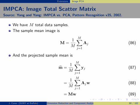
Extensions Image PCA
IMPCA: Image Total Scatter MatrixSource: Yang and Yang: IMPCA vs. PCA, Pattern Recognition v35, 2002.
We have M total data samples.
The sample mean image is
M =1
M
M∑
j=1
Aj (86)
And the projected sample mean is
m̃ =1
M
M∑
j=1
yj (87)
=1
M
M∑
j=1
Ajw (88)
= Mw (89)
J. Corso (SUNY at Buffalo) Dimension Reduction and Component Analysis 80 / 102
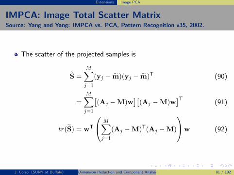
Extensions Image PCA
IMPCA: Image Total Scatter MatrixSource: Yang and Yang: IMPCA vs. PCA, Pattern Recognition v35, 2002.
The scatter of the projected samples is
S̃ =
M∑
j=1
(yj − m̃)(yj − m̃)T (90)
=
M∑
j=1
[(Aj −M)w
][(Aj −M)w
]T(91)
tr(S̃) = wT
M∑
j=1
(Aj −M)T(Aj −M)
w (92)
J. Corso (SUNY at Buffalo) Dimension Reduction and Component Analysis 81 / 102

Extensions Image PCA
IMPCA: Image Total Scatter MatrixSource: Yang and Yang: IMPCA vs. PCA, Pattern Recognition v35, 2002.
So, the image total scatter matrix is
SI =
M∑
j=1
(Aj −M)T(Aj −M) (93)
And, a suitable criterion, in a form we’ve seen before is
JI(w) = wTSIw (94)
We know already that the vectors w that maximize JI are theorthonormal eigenvectors of SI corresponding to the largesteigenvalues of SI .
J. Corso (SUNY at Buffalo) Dimension Reduction and Component Analysis 82 / 102

Extensions Image PCA
IMPCA: Experimental ResultsSource: Yang and Yang: IMPCA vs. PCA, Pattern Recognition v35, 2002.
Dataset is the ORL database
10 different images taken of 40 individuals.Facial expressions and details are varying.Even the pose can vary slightly: 20 degree rotation/tilt and 10% scale.Size is normalized (92× 112).
1998 J. Yang, J.-Y. Yang / Pattern Recognition 35 (2002) 1997–1999
where, TSx denotes the total covariance matrix of projectedfeature vectors of training images, and tr(TSx) denotes thetrace of TSx. Now, the problem is how to evaluate the co-variance matrix TSx.
Suppose there are L known pattern classes, andM denotesthe total number of samples of all classes. The jth trainingimage is denoted by an m × n matrix Aj (j = 1; 2; : : : ; M),and the mean image of all training sample is denoted by KA.
After the projection of training image onto X , we get theprojected feature vector
Yj = AjX; j = 1; 2; : : : ; M: (3)
Suppose the mean vector of all projected feature vectors isdenoted by KY , it is easy to get KY = KAX . Then, TSx can beevaluated by
TSx =1M
M∑
j=1
(Yj − KY )(Yj − KY )T
=1M
M∑
j=1
[(Aj − KA)X ][(Aj − KA)X ]T: (4)
So
tr(TSx) = X T
(1M
M∑
j=1
(Aj − KA)T(Aj − KA)
)X: (5)
Now, let us de<ne the matrix below
Gt =1M
M∑
j=1
(Aj − KA)T(Aj − KA): (6)
The matrix Gt is called image total covariance (scatter)matrix. And, it is easy to verify that Gt is an n× n nonneg-ative de<nite matrix by its de<nition.
Accordingly, the criterion in Eq. (2) can be expressed inthis form
Jp(X ) = X TGtX: (7)
2.2. Image principal component analysis
The criterion in Eq. (7) is called generalized total scattercriterion. In fact, in the special case of image matrix beingrow vectors, it is not hard to prove that the criterion is thecommon total scatter criterion. The vector X maximizing thecriterion is called the optimal projection axe, and its physicalmeaning is obvious, i.e., after projection of image matrixonto X , the total scatter of projected samples is maximized.
It is evident that the optimal projection axe is the eigen-vector corresponding to the maximal eigenvalue of Gt . Gen-erally, in many cases, one optimal projection axe is notenough, we usually select a set of projection axes subjectto the orthonormal constraints and maximizing the criterionin Eq. (7). In fact, the optimal projection axes X1; : : : ; Xd ofIMPCA can be selected as the orthonormal eigenvectors ofGt associated with the <rst d largest eigenvalues.
Fig. 1. Five images of one person in ORL face database.
2.3. Feature extraction method
The obtained optimal projection vectors X1; : : : ; Xd of IM-PCA are used for feature extraction. Let
Yk = AXk ; k = 1; 2; : : : ; d: (8)
Then, we get a family of image projected feature vectorsY1; : : : ; Yd, which are used to form an N = md dimensionalresulting projected feature vector of image A as follows:
Y =
Y1
Y2
...
Yd
=
AX1
AX2
...
AXd
: (9)
3. Experimental results
The proposed method is tested on the ORL database thatcontains a set of face images taken at the Olivetti ResearchLaboratory in Cambridge, UK. There are 10 diOerent imagesfor 40 individuals. For some persons, the images were takenat diOerent times. And the facial expression (open=closedeyes, smiling=non-smiling) and facial details (glasses=noglasses) are variable. The images were taken against a darkhomogeneous background and the persons are in upright,frontal position with tolerance for some tilting and rotationof up to 20◦. Moreover, there is some variation in scale ofup to about 10%. All images are grayscale and normalizedwith a resolution of 92×112. The <ve images of one personin ORL are shown in Fig. 1.
In this experiment, we use the <rst <ve images of eachperson for training and the remaining <ve for testing. Thusthe total amount of training samples and testing samples areboth 200. The proposed IMPCA is used for feature extrac-tion. Here, since the size of image total covariance matrixGt is 92 × 92, it is very easy to work out its eigenvectors.And the number of selected eigenvectors (projection vec-tors) varies from 1 to 10. Note that if the projection vectornumber is k, the dimension of corresponding projected fea-ture vector is 112×k. Finally, a minimum distance classi<erand a nearest neighbor classi<er are, respectively, employedto classify in the projected feature space. The recognitionrates are shown in Table 1. The Eigenfaces [1] and Fisher-faces [2] are used for feature extraction as well, and theiroptimal performance lies in Table 2. Moreover, the CPU
The first five images of each person are used for training and thesecond five are used for testing.
J. Corso (SUNY at Buffalo) Dimension Reduction and Component Analysis 83 / 102

Extensions Image PCA
IMPCA: Experimental ResultsSource: Yang and Yang: IMPCA vs. PCA, Pattern Recognition v35, 2002.
IMPCA varying the number of extracted eigenvectors (NN classifier):
J. Yang, J.-Y. Yang / Pattern Recognition 35 (2002) 1997–1999 1999
Table 1Recognition rates (%) based on IMPCA projected features as the number of projection vectors varying from 1 to 10
Projection 1 2 3 4 5 6 7 8 9 10vector number
Minimum distance 73.0 83.0 86.5 88.5 88.5 88.5 90.0 90.5 91.0 91.0Nearest neighbor 85.0 92.0 93.5 94.5 94.5 95.0 95.0 95.5 93.5 94.0
Table 2Comparison of the maximal recognition rates using the three meth-ods
Recognition rate Eigenfaces Fisherfaces IMPCA
Minimum distance 89.5% (46) 88.5% (39) 91.0%Nearest neighbor 93.5% (37) 88.5% (39) 95.5%
Note: The value in parentheses denotes the number of axes asthe maximal recognition rate is achieved.
Table 3The CPU time consumed for feature extraction and classi<cationusing the three methods
Time (s) Feature Classi<cation Totalextraction time time time
Eigenfaces (37) 371.79 5.16 376.95Fisherfaces (39) 378.10 5.27 383.37IMPCA (112 × 8) 27.14 25.04 52.18
time consumed for feature extraction and classi<cation usingthe above methods under a nearest neighbor classi<er isexhibited in Table 3.
Tables 1 and 2 indicate that our proposed IMPCA outper-forms Eigenfaces and Fisherfaces. What’s more, in Table 3,it is evident that the time consumed for feature extractionusing IMPCA is much less than that of the other two meth-ods. So our methods are more preferable for image featureextraction.
Acknowledgements
We wish to thank National Science Foundation of Chinaunder Grant No.60072034 for supporting.
References
[1] M. Turk, A. Pentland, Face recognition using Eigenfaces,Proceedings of the IEEE Conference on Computer Vision andPattern Recognition, 1991, pp. 586–591.
[2] P.N. Belhumeur, J.P. Hespanha, D.J. Kriengman, Eigenfaces vs.Fisherfaces: recognition using class speci<c linear projection,IEEE Trans. Pattern Anal. Mach. Intell. 19 (7) (1997) 711–720.
[3] K. Liu, Y.-Q. Cheng, J.-Y. Yang, et al., Algebraic featureextraction for image recognition based on an optimaldiscriminant criterion, Pattern Recognition 26 (6) (1993)903–911.
About the Author—JIAN YANG was born in Jiangsu, China, on 3 June 1973. He received his M.S. degree in Applied Mathematics fromChangsha Railway University in 1998. Now, he is a teacher in the Department of Applied Mathematics of Nanjing University of Scienceand Technology (NUST). At the same time, he is working for his Ph.D. degree in Pattern Recognition and Intelligence System. His currentinterests include face recognition and detection, handwritten character recognition and data fusion.
About the Author—JING-YU YANG received the B.S. Degree in Computer Science from NUST, Nanjing, China. From 1982 to 1984 hewas a visiting scientist at the Coordinated Science Laboratory, University of Illinois at Urbana-Champaign. From 1993 to 1994 he was avisiting professor at the Department of Computer Science, Missuria University. And in 1998, he acted as a visiting professor at ConcordiaUniversity in Canada. He is currently a professor and Chairman in the department of Computer Science at NUST. He is the author ofover 100 scienti<c papers in computer vision, pattern recognition, and arti<cial intelligence. He has won more than 20 provincial awardsand national awards. His current research interests are in the areas of pattern recognition, robot vision, image processing, data fusion, andarti<cial intelligence.
J. Corso (SUNY at Buffalo) Dimension Reduction and Component Analysis 84 / 102

Extensions Image PCA
IMPCA: Experimental ResultsSource: Yang and Yang: IMPCA vs. PCA, Pattern Recognition v35, 2002.
IMPCA vs. EigenFaces vs. FisherFaces for Recognition
J. Yang, J.-Y. Yang / Pattern Recognition 35 (2002) 1997–1999 1999
Table 1Recognition rates (%) based on IMPCA projected features as the number of projection vectors varying from 1 to 10
Projection 1 2 3 4 5 6 7 8 9 10vector number
Minimum distance 73.0 83.0 86.5 88.5 88.5 88.5 90.0 90.5 91.0 91.0Nearest neighbor 85.0 92.0 93.5 94.5 94.5 95.0 95.0 95.5 93.5 94.0
Table 2Comparison of the maximal recognition rates using the three meth-ods
Recognition rate Eigenfaces Fisherfaces IMPCA
Minimum distance 89.5% (46) 88.5% (39) 91.0%Nearest neighbor 93.5% (37) 88.5% (39) 95.5%
Note: The value in parentheses denotes the number of axes asthe maximal recognition rate is achieved.
Table 3The CPU time consumed for feature extraction and classi<cationusing the three methods
Time (s) Feature Classi<cation Totalextraction time time time
Eigenfaces (37) 371.79 5.16 376.95Fisherfaces (39) 378.10 5.27 383.37IMPCA (112 × 8) 27.14 25.04 52.18
time consumed for feature extraction and classi<cation usingthe above methods under a nearest neighbor classi<er isexhibited in Table 3.
Tables 1 and 2 indicate that our proposed IMPCA outper-forms Eigenfaces and Fisherfaces. What’s more, in Table 3,it is evident that the time consumed for feature extractionusing IMPCA is much less than that of the other two meth-ods. So our methods are more preferable for image featureextraction.
Acknowledgements
We wish to thank National Science Foundation of Chinaunder Grant No.60072034 for supporting.
References
[1] M. Turk, A. Pentland, Face recognition using Eigenfaces,Proceedings of the IEEE Conference on Computer Vision andPattern Recognition, 1991, pp. 586–591.
[2] P.N. Belhumeur, J.P. Hespanha, D.J. Kriengman, Eigenfaces vs.Fisherfaces: recognition using class speci<c linear projection,IEEE Trans. Pattern Anal. Mach. Intell. 19 (7) (1997) 711–720.
[3] K. Liu, Y.-Q. Cheng, J.-Y. Yang, et al., Algebraic featureextraction for image recognition based on an optimaldiscriminant criterion, Pattern Recognition 26 (6) (1993)903–911.
About the Author—JIAN YANG was born in Jiangsu, China, on 3 June 1973. He received his M.S. degree in Applied Mathematics fromChangsha Railway University in 1998. Now, he is a teacher in the Department of Applied Mathematics of Nanjing University of Scienceand Technology (NUST). At the same time, he is working for his Ph.D. degree in Pattern Recognition and Intelligence System. His currentinterests include face recognition and detection, handwritten character recognition and data fusion.
About the Author—JING-YU YANG received the B.S. Degree in Computer Science from NUST, Nanjing, China. From 1982 to 1984 hewas a visiting scientist at the Coordinated Science Laboratory, University of Illinois at Urbana-Champaign. From 1993 to 1994 he was avisiting professor at the Department of Computer Science, Missuria University. And in 1998, he acted as a visiting professor at ConcordiaUniversity in Canada. He is currently a professor and Chairman in the department of Computer Science at NUST. He is the author ofover 100 scienti<c papers in computer vision, pattern recognition, and arti<cial intelligence. He has won more than 20 provincial awardsand national awards. His current research interests are in the areas of pattern recognition, robot vision, image processing, data fusion, andarti<cial intelligence.
IMPCA vs. EigenFaces vs. FisherFaces for Speed
J. Yang, J.-Y. Yang / Pattern Recognition 35 (2002) 1997–1999 1999
Table 1Recognition rates (%) based on IMPCA projected features as the number of projection vectors varying from 1 to 10
Projection 1 2 3 4 5 6 7 8 9 10vector number
Minimum distance 73.0 83.0 86.5 88.5 88.5 88.5 90.0 90.5 91.0 91.0Nearest neighbor 85.0 92.0 93.5 94.5 94.5 95.0 95.0 95.5 93.5 94.0
Table 2Comparison of the maximal recognition rates using the three meth-ods
Recognition rate Eigenfaces Fisherfaces IMPCA
Minimum distance 89.5% (46) 88.5% (39) 91.0%Nearest neighbor 93.5% (37) 88.5% (39) 95.5%
Note: The value in parentheses denotes the number of axes asthe maximal recognition rate is achieved.
Table 3The CPU time consumed for feature extraction and classi<cationusing the three methods
Time (s) Feature Classi<cation Totalextraction time time time
Eigenfaces (37) 371.79 5.16 376.95Fisherfaces (39) 378.10 5.27 383.37IMPCA (112 × 8) 27.14 25.04 52.18
time consumed for feature extraction and classi<cation usingthe above methods under a nearest neighbor classi<er isexhibited in Table 3.
Tables 1 and 2 indicate that our proposed IMPCA outper-forms Eigenfaces and Fisherfaces. What’s more, in Table 3,it is evident that the time consumed for feature extractionusing IMPCA is much less than that of the other two meth-ods. So our methods are more preferable for image featureextraction.
Acknowledgements
We wish to thank National Science Foundation of Chinaunder Grant No.60072034 for supporting.
References
[1] M. Turk, A. Pentland, Face recognition using Eigenfaces,Proceedings of the IEEE Conference on Computer Vision andPattern Recognition, 1991, pp. 586–591.
[2] P.N. Belhumeur, J.P. Hespanha, D.J. Kriengman, Eigenfaces vs.Fisherfaces: recognition using class speci<c linear projection,IEEE Trans. Pattern Anal. Mach. Intell. 19 (7) (1997) 711–720.
[3] K. Liu, Y.-Q. Cheng, J.-Y. Yang, et al., Algebraic featureextraction for image recognition based on an optimaldiscriminant criterion, Pattern Recognition 26 (6) (1993)903–911.
About the Author—JIAN YANG was born in Jiangsu, China, on 3 June 1973. He received his M.S. degree in Applied Mathematics fromChangsha Railway University in 1998. Now, he is a teacher in the Department of Applied Mathematics of Nanjing University of Scienceand Technology (NUST). At the same time, he is working for his Ph.D. degree in Pattern Recognition and Intelligence System. His currentinterests include face recognition and detection, handwritten character recognition and data fusion.
About the Author—JING-YU YANG received the B.S. Degree in Computer Science from NUST, Nanjing, China. From 1982 to 1984 hewas a visiting scientist at the Coordinated Science Laboratory, University of Illinois at Urbana-Champaign. From 1993 to 1994 he was avisiting professor at the Department of Computer Science, Missuria University. And in 1998, he acted as a visiting professor at ConcordiaUniversity in Canada. He is currently a professor and Chairman in the department of Computer Science at NUST. He is the author ofover 100 scienti<c papers in computer vision, pattern recognition, and arti<cial intelligence. He has won more than 20 provincial awardsand national awards. His current research interests are in the areas of pattern recognition, robot vision, image processing, data fusion, andarti<cial intelligence.
J. Corso (SUNY at Buffalo) Dimension Reduction and Component Analysis 85 / 102

Extensions Image PCA
IMPCA: DiscussionSource: Yang and Yang: IMPCA vs. PCA, Pattern Recognition v35, 2002.
There is a clear speed-up because the amount of computation hasbeen greatly reduced.
However, this speed-up comes at some cost. What is that cost?
Why does IMPCA work in this case?
What is IMPCA really doing?
J. Corso (SUNY at Buffalo) Dimension Reduction and Component Analysis 86 / 102

Non-linear Dimension Reduction Locally Linear Embedding
Locally Linear EmbeddingSource: Saul and Roweis, An Introduction to Locally Linear Embedding, 2001
So far, we have covered a few methods for dimension reduction thatall make the underlying assumption the data in high dimension liveson a planar manifold in the lower dimension.
The methods are easy to implement.The methods do not suffer from local minima.
But, what if the data is non-linear?
the top eigenvectorsof thedatacovariancematrix. In classical(or metric)MDS,one computesthe low dimensionalembeddingthat bestpreserves pairwisedis-tancesbetweendatapoints. If thesedistancescorrespondto Euclideandistances,the resultsof metric MDS are equivalent to PCA. Both methodsare simple toimplement,andtheir optimizationsdo not involve localminima.Thesevirtuesac-countfor thewidespreaduseof PCA andMDS, despitetheir inherentlimitationsaslinearmethods.
Recently, we introducedaneigenvectormethod—calledlocally linearembedding(LLE)—for the problemof nonlineardimensionalityreduction[4]. This problemis illustratedby the nonlinearmanifold in Figure1. In this example,the dimen-sionalityreductionby LLE succeedsin identifying theunderlyingstructureof themanifold,while projectionsof thedataby PCA or metricMDS mapfaraway datapointsto nearbypointsin the plane. Like PCA andMDS, our algorithmis sim-ple to implement,andits optimizationsdo not involve local minima. At thesametime, however, it is capableof generatinghighly nonlinearembeddings.Notethatmixturemodelsfor localdimensionalityreduction[5, 6], whichclusterthedataandperformPCA within eachcluster, do not addressthe problemconsideredhere—namely, how to maphigh dimensionaldatainto a singleglobalcoordinatesystemof lowerdimensionality.
In this paper, we review theLLE algorithmin its mostbasicform andillustrateapotentialapplicationto audiovisualspeechsynthesis[3].
-1 0 1 0
5-1
0
1
2
3
(A)
-1 0 1 0
5-1
0
1
2
3
(B)
-2 -1 0 1 2-2
-1
0
1
2
(C)
Figure 1: The problemof nonlineardimensionalityreduction,as illustratedforthreedimensionaldata(B) sampledfrom a two dimensionalmanifold(A). An un-supervisedlearningalgorithmmustdiscover theglobal internalcoordinatesof themanifold without signalsthat explicitly indicatehow the datashouldbe embed-dedin two dimensions.Theshadingin (C) illustratestheneighborhood-preservingmappingdiscoveredby LLE.
2
J. Corso (SUNY at Buffalo) Dimension Reduction and Component Analysis 87 / 102
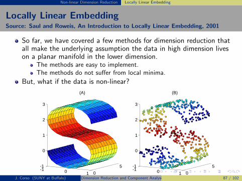

Non-linear Dimension Reduction Locally Linear Embedding
The Non-Linear ProblemSource: Saul and Roweis, An Introduction to Locally Linear Embedding, 2001
In non-linear dimension reduction, one must discover the globalinternal coordinates of the manifold without signals that explicitlyindicate how the data should be embedded in the lower dimension (oreven how many dimensions should be used).
The LLE way of doing this is to make the assumption that, givenenough data samples, the local frame of a particular point xi is linear.LLE proceeds to preserve this local structure while simultaneouslyreducing the global dimension (indeed preserving the local structuregives LLE the necessary constraints to discover the manifold).
J. Corso (SUNY at Buffalo) Dimension Reduction and Component Analysis 88 / 102

Non-linear Dimension Reduction Locally Linear Embedding
LLE: NeighborhoodsSource: Saul and Roweis, An Introduction to Locally Linear Embedding, 2001
Suppose we have n real-valued vectors xi in dataset D each ofdimension D. We assume these data are sampled from some smoothunderlying manifold.
Furthermore, we assume that each data point and its neighbors lie onor close to a locally linear patch of the manifold.
LLE characterizes the local geometry of these patches by linearcoefficients that reconstruct each data point from its neighbors.
If the neighbors form the D-dimensional simplex, then thesecoefficients form the barycentric coordinates of the data point.In the simplest form of LLE, one identifies K such nearest neighborsbased on the Euclidean distance.But, one can use all points in a ball of fixed radius, or even moresophisticated metrics.
J. Corso (SUNY at Buffalo) Dimension Reduction and Component Analysis 89 / 102

Non-linear Dimension Reduction Locally Linear Embedding
LLE: NeighborhoodsSource: Saul and Roweis, An Introduction to Locally Linear Embedding, 2001
We can write down the reconstruction error with the following costfunction:
JLLE1(W) =∑
i
∣∣∣∣xi −∑
j
Wijxj
∣∣∣∣2
(95)
Notice that each row of the weight matrix W will be nonzero for onlyK columns; i.e., W is a quite sparse matrix. I.e., if we define the setN(xi) as the K neighbors of xi, then we enforce
Wij = 0 if xj /∈ N(xi) (96)
We will enforce that the rows sum to 1, i.e.,∑
jWij = 1. (This is forinvariance.)
J. Corso (SUNY at Buffalo) Dimension Reduction and Component Analysis 90 / 102

Non-linear Dimension Reduction Locally Linear Embedding
LLE: NeighborhoodsSource: Saul and Roweis, An Introduction to Locally Linear Embedding, 2001
Note that the constrained weights that minimize these reconstructionerrors obey important symmetries: for any data point, they areinvariant to rotations, rescalings, and translations of that data pointand its neighbors.
This means that these weights characterize intrinsic geometricproperties of the neighborhood as opposed to any properties thatdepend on a particular frame of reference.
If we suppose the data lie on or near a smooth nonlinear manifold ofdimension d� D. Then, to a good approximation, there exists alinear mapping (a translation, rotation, and scaling) that maps thehigh dimensional coordinates of each neighborhood to global internalcoordinates on the manifold.
J. Corso (SUNY at Buffalo) Dimension Reduction and Component Analysis 91 / 102

Non-linear Dimension Reduction Locally Linear Embedding
LLE: NeighborhoodsSource: Saul and Roweis, An Introduction to Locally Linear Embedding, 2001
So, we expect that the characterization of the local neighborhoods(W) in the original space to be equally valid for the local patches onthe manifold.
In other words, the same weights Wij that reconstruct point xi in theoriginal space should also reconstruct it in the embedded manifoldcoordinate system.
First, let’s solve for the weights. And, then we’ll see how to use thispoint to ultimately compute the global dimension reduction.
J. Corso (SUNY at Buffalo) Dimension Reduction and Component Analysis 92 / 102

Non-linear Dimension Reduction Locally Linear Embedding
Solving for the WeightsSource: Saul and Roweis, An Introduction to Locally Linear Embedding, 2001
Solving for the weights W is a constrained least-squares problem.
Consider a particular x with K nearest neighbors ηj and weights wjwhich sum to one. We can write the reconstruction error as
ε =
∣∣∣∣x−∑
j
wjηj
∣∣∣∣2
(97)
=
∣∣∣∣∑
j
wj(x− ηj)
∣∣∣∣2
(98)
=∑
jk
wjwkCjk (99)
where Cjk is the covariance (x− ηj)(x− ηk)T.
J. Corso (SUNY at Buffalo) Dimension Reduction and Component Analysis 93 / 102

Non-linear Dimension Reduction Locally Linear Embedding
Solving for the WeightsSource: Saul and Roweis, An Introduction to Locally Linear Embedding, 2001
We need to add a Lagrange multiplier to enforce the constraint∑j wj = 1 and then the weights can be solved in closed form.
The optimal weights, in terms of the local covariance matrix, are
wj =
∑k C−1jk∑
lmC−1lm
. (100)
But, rather than explicitly inverting the covariance matrix, one cansolve the linear system
∑
k
Cjkwk = 1 (101)
and rescale the weights so that they sum to one.
J. Corso (SUNY at Buffalo) Dimension Reduction and Component Analysis 94 / 102

Non-linear Dimension Reduction Locally Linear Embedding
Stage 2: Neighborhood Preserving MappingSource: Saul and Roweis, An Introduction to Locally Linear Embedding, 2001
Each high-dimensional input vector xi is mapped to a low-dimensionvector yi representing the global internal coordinates on the manifold.
LLE does this by choosing the d-dimension coordinates yi tominimize the embedding cost function:
JLLE2(y) =∑
i
∣∣∣∣yi −∑
j
Wijyj
∣∣∣∣2
(102)
The basis for the cost function is the same—locally linearreconstruction errors—but here, the weights W are fixed and thecoordinates y are optimized.
J. Corso (SUNY at Buffalo) Dimension Reduction and Component Analysis 95 / 102

Non-linear Dimension Reduction Locally Linear Embedding
Stage 2: Neighborhood Preserving MappingSource: Saul and Roweis, An Introduction to Locally Linear Embedding, 2001
This defines a quadratic:
JLLE2(y) =∑
i
∣∣∣∣yi −∑
j
Wijyj
∣∣∣∣2
(103)
=∑
ij
Mij(yTi yj) (104)
where
Mij = δij −Wij −Wji +∑
k
WkiWkj (105)
with δij is 1 if j 6= i and 0 otherwise.
J. Corso (SUNY at Buffalo) Dimension Reduction and Component Analysis 96 / 102

Non-linear Dimension Reduction Locally Linear Embedding
Stage 2: Neighborhood Preserving MappingSource: Saul and Roweis, An Introduction to Locally Linear Embedding, 2001
To remove the degree of freedom for translation, we enforce thecoordinates to be centered at the origin:
∑
i
yi = 0 (106)
To avoid degenerate solutions, we constrain the embedding vectors tohave unit covariance, with their outer-products satisfying
1
n
∑
i
yiyTi = I (107)
The optimal embedding is found by the bottom d+ 1 non-zeroeigenvectors, i.e., those d+ 1 eigenvectors corresponding to thesmallest but non-zero d+ 1 eigenvalues. The bottom eigenvector isthe unit vector the corresponds to the free translation, it is discarded.
J. Corso (SUNY at Buffalo) Dimension Reduction and Component Analysis 97 / 102

Non-linear Dimension Reduction Locally Linear Embedding
Putting It TogetherSource: Saul and Roweis, An Introduction to Locally Linear Embedding, 2001
LLE ALGORITHM
1. Computetheneighborsof eachdatapoint,�� �
.
2. Computetheweights � �
thatbestreconstructeachdatapoint�� �
fromits neighbors,minimizing thecostin eq.(1) by constrainedlinearfits.
3. Computethevectors�$/�
bestreconstructedby theweights � �
, minimizingthequadraticform in eq.(2) by its bottomnonzeroeigenvectors.
Figure2: Summaryof theLLE algorithm,mappinghigh dimensionaldatapoints,����, to low dimensionalembeddingvectors,
�$0�.
arechosen,theoptimalweights � �
andcoordinates$ �
arecomputedby standardmethodsin linearalgebra.Thealgorithminvolvesa singlepassthroughthethreestepsin Fig. 2 andfindsglobalminimaof thereconstructionandembeddingcostsin Eqs.(1) and(2). As discussedin AppendixA, in the unusualcasewheretheneighborsoutnumbertheinputdimensionality
� �213� � , theleastsquaresproblemfor findingtheweightsdoesnothaveauniquesolution,andaregularizationterm—for example,onethatpenalizesthesquaredmagnitudesof the weights—mustbeaddedto thereconstructioncost.
Thealgorithm,asdescribedin Fig. 2, takesasinput the�
high dimensionalvec-tors,
�� �. In many settings,however, theusermay not have accessto dataof this
form, but only to measurementsof dissimilarityor pairwisedistancebetweendif-ferentdatapoints. A simplevariationof LLE, describedin AppendixC, canbeappliedto input of this form. In this way, matricesof pairwisedistancescanbeanalyzedby LLE just aseasilyasMDS[2]; in factonly a smallfractionof all pos-sible pairwisedistances(representingdistancesbetweenneighboringpoints andtheir respective neighbors)arerequiredfor runningLLE.
3 Examples
The embeddingsdiscoveredby LLE areeasiestto visualizefor intrinsically twodimensionalmanifolds.In Fig.1, for example,theinputtoLLE consisted
� �546�7�datapointssampledoff the S-shapedmanifold. The resultingembeddingshowshow thealgorithm,using � �8 :9
neighborsperdatapoint,successfullyunraveledtheunderlyingtwo dimensionalstructure.
5
LLE illustrates a general principle of manifold learning, elucidated byTenenbaum et al[11], that overlapping local neighborhoods—collectivelyanalyzed—can provide information about global geometry. (From Saul andRoweis 2001)
J. Corso (SUNY at Buffalo) Dimension Reduction and Component Analysis 98 / 102

Non-linear Dimension Reduction Locally Linear Embedding
Example 1Source: Saul and Roweis, An Introduction to Locally Linear Embedding, 2001
K=12.
the top eigenvectorsof thedatacovariancematrix. In classical(or metric)MDS,one computesthe low dimensionalembeddingthat bestpreserves pairwisedis-tancesbetweendatapoints. If thesedistancescorrespondto Euclideandistances,the resultsof metric MDS are equivalent to PCA. Both methodsare simple toimplement,andtheir optimizationsdo not involve localminima.Thesevirtuesac-countfor thewidespreaduseof PCA andMDS, despitetheir inherentlimitationsaslinearmethods.
Recently, we introducedaneigenvectormethod—calledlocally linearembedding(LLE)—for the problemof nonlineardimensionalityreduction[4]. This problemis illustratedby the nonlinearmanifold in Figure1. In this example,the dimen-sionalityreductionby LLE succeedsin identifying theunderlyingstructureof themanifold,while projectionsof thedataby PCA or metricMDS mapfaraway datapointsto nearbypointsin the plane. Like PCA andMDS, our algorithmis sim-ple to implement,andits optimizationsdo not involve local minima. At thesametime, however, it is capableof generatinghighly nonlinearembeddings.Notethatmixturemodelsfor localdimensionalityreduction[5, 6], whichclusterthedataandperformPCA within eachcluster, do not addressthe problemconsideredhere—namely, how to maphigh dimensionaldatainto a singleglobalcoordinatesystemof lowerdimensionality.
In this paper, we review theLLE algorithmin its mostbasicform andillustrateapotentialapplicationto audiovisualspeechsynthesis[3].
-1 0 1 0
5-1
0
1
2
3
(A)
-1 0 1 0
5-1
0
1
2
3
(B)
-2 -1 0 1 2-2
-1
0
1
2
(C)
Figure 1: The problemof nonlineardimensionalityreduction,as illustratedforthreedimensionaldata(B) sampledfrom a two dimensionalmanifold(A). An un-supervisedlearningalgorithmmustdiscover theglobal internalcoordinatesof themanifold without signalsthat explicitly indicatehow the datashouldbe embed-dedin two dimensions.Theshadingin (C) illustratestheneighborhood-preservingmappingdiscoveredby LLE.
2
J. Corso (SUNY at Buffalo) Dimension Reduction and Component Analysis 99 / 102

Non-linear Dimension Reduction Locally Linear Embedding
Example 2Source: Saul and Roweis, An Introduction to Locally Linear Embedding, 2001
K=4.
Figure3: Theresultsof PCA(top)andLLE (bottom),appliedto imagesof asingleface translatedacrossa two-dimensionalbackgroundof noise. Note how LLEmapstheimageswith cornerfacesto thecornersof its twodimensionalembedding,while PCA fails to preserve theneighborhoodstructureof nearbyimages.
7
J. Corso (SUNY at Buffalo) Dimension Reduction and Component Analysis 100 / 102

Non-linear Dimension Reduction Locally Linear Embedding
Example 3Source: Saul and Roweis, An Introduction to Locally Linear Embedding, 2001
K=16.
Figure4: Imagesof lips mappedinto theembeddingspacedescribedby thefirsttwo coordinatesof PCA (top) andLLE (bottom). Representative lips areshownnext to circledpointsin differentpartsof eachspace.Thedifferencesbetweenthetwo embeddingsindicatethepresenceof nonlinearstructurein thedata.
8
Figure4: Imagesof lips mappedinto theembeddingspacedescribedby thefirsttwo coordinatesof PCA (top) andLLE (bottom). Representative lips areshownnext to circledpointsin differentpartsof eachspace.Thedifferencesbetweenthetwo embeddingsindicatethepresenceof nonlinearstructurein thedata.
8
If the lip images described a nearly linear manifold, these two methods would
yield similar results; thus the significant differences in these embeddings reveal the
presence of nonlinear structure.J. Corso (SUNY at Buffalo) Dimension Reduction and Component Analysis 101 / 102

Non-linear Dimension Reduction Locally Linear Embedding
LLE ComplexitySource: Saul and Roweis, An Introduction to Locally Linear Embedding, 2001
Computing nearest neighbors scales O(Dn2) in the worst case. But,in many situations, space partitioning methods can be used to findthe K nearest neighbors in O(n log n) time.
Computing the weights is O(DnK3).
Computing the projection is O(dn2).
All matrix computations are on very sparse matrices and can thus beimplemented quite efficiently.
J. Corso (SUNY at Buffalo) Dimension Reduction and Component Analysis 102 / 102