dimensionality reduction for similarity searching … reduction for similarity searching in dynamic...

Dimensionality Reduction for Similarity Searching in Dynamic Databases

K. V. Ravi Kanth Divyakant Agrawal Amr El Abbadi

Ambuj Singh�kravi, agrawal, ambuj � @cs.ucsb.edu

Department of Computer Science

University of California at Santa Barbara

Santa Barbara, CA 93106

Abstract

Databases are increasingly being used to store multi-media objects such as maps, images, audio and video. Storage

and retrieval of these objects is accomplished using multi-dimensional index structures such as R � -trees and SS-trees.

As dimensionality increases, query performance in these index structures degrades. This phenomenon, generally

referred to as the dimensionality curse, can be circumvented by reducing the dimensionality of the data. Such a

reduction is however accompanied by a loss of precision of query results. Current techniques such as QBIC use SVD

transform-based dimensionality reduction to ensure high query precision. The drawback of this approach is that SVD

is expensive to compute, and therefore not readily applicable to dynamic databases. In this paper, we propose novel

techniques for performing SVD-based dimensionality reduction in dynamic databases. When the data distribution

changes considerably so as to degrade query precision, we recompute the SVD transform and incorporate it in the

existing index structure. For recomputing the SVD-transform, we propose a novel technique that uses aggregate

data from the existing index rather than the entire data. This technique reduces the SVD-computation time without

compromising query precision. We then explore efficient ways to incorporate the recomputed SVD-transform in the

existing index structure without degrading subsequent query response times. These techniques reduce the computation

time by a factor of 20 in experiments on color and texture image vectors. The error due to approximate computation

of SVD is less than 10%.

1 Introduction

Rapid advances in information technology have opened up new frontiers for research and development in the past

decade. One such area is the storage and management of multi-media objects such as maps, images, text, audio and

video. A natural approach for retrieving such multi-media objects is by their content. In this content-based retrieval,

data objects similar in content to a query object are retrieved. Over the years, such content-based retrieval of images,

1

video, audio text and time sequences has received much attention in the database community. To support such similar-

ity queries, similarity metrics between different objects are maintained in the database. For most applications such as

images, text or time sequences, the similarity metrics can be embedded in a high-dimensional vector space. Proximity

in the high-dimensional vector space reflects the similarity of the content of the data objects in these applications. For

instance, the color content of images may be described by the percentage of pixels in the image that have a particu-

lar color. The different possible colors form different dimensions, and the computed color fractions form the values

along these dimensions. Given this transformation, a request for images similar to a query image can be answered by

searching in the proximity of the query image in the high-dimensional space. This approach for content-based retrieval

reduces the problem to one of searching in high-dimensional space. In this paper, we explore how to support this type

of search efficiently for dynamic databases, where objects may be inserted and deleted frequently.

Searching in multiple dimensions has been extensively researched in the database and computational geometry

literature. Several data structures such as R-trees [1, 2, 13], hB-trees [18], Bang files [7, 8, 9], TV-trees [17], SS-

trees [24], and SR-trees [16] are designed for supporting fast searching in large multi-dimensional databases. These

structures are quite efficient for small dimensions (of the order of 1-10). However, as the data dimensionality increases,

the query performance of these structures degrades rapidly. For instance, White and Jain [24] report that as the

dimensionality increases from 5 to 10, the performance of a nearest-neighbor query in multi-dimensional structures

such as the SS-tree [24] and the R � -tree [1], degrades by a factor of 12. This phenomenon, appropriately termed

the dimensionality curse by Agrawal and Faloutsos [6], is a common characteristic of all multi-dimensional index

structures. In spite of the progress in the design and analysis of multi-dimensional structures such as the TV-trees [17],

the X-trees [2], the SS-trees [24], and the SR-trees [16], the dimensionality curse persists.

The only known solution for achieving scalable query performance is by reducing the dimensionality of the data.

Several research initiatives [5, 14, 17, 20, 21] including the QBIC project adopt this approach for supporting image

retrieval based on their content. This approach for content-based retrieval first condenses most of the information

in a dataset to a few dimensions by applying Singular Value Decomposition (SVD). The data in the few condensed

dimensions are then indexed to support fast retrieval based on their color, texture or shape content. This approach

assumes that the SVD is computed a priori on the entire data. Therefore, it works only for static databases and is

not applicable to dynamic databases. In this paper, we focus on dynamic databases, where the SVD needs to be

recomputed due to changes in the underlying data. We propose a novel technique to efficiently recompute SVD for

such dynamic environments.

Much research has been done on updating SVD as new vectors are added to, and old ones deleted from a database

[3, 4, 12, 19]. A simple technique [11] for computing SVD after a new item is added to a database of �� -dimensional

vectors has �� time complexity. However, incremental techniques [3, 4] reduce this complexity to �� ,where � is the rank of the matrix of the � � -dimensional vectors ( � is usually much smaller than � ). Although these

techniques reduce the multiplicative factor from �� to �� ), the time complexity is still linear in the number of

vectors � . In this paper, we propose a novel approach to reduce this linear dependence: instead of using the entire set

of � vectors, we use an aggregate data set of � vectors, �� , to recompute the SVD. This technique reduces the

recomputation time, irrespective of the SVD update algorithm used. The quality of the recomputed SVD depends on

how well the aggregate data set reflects the data distribution. We ensure this by obtaining the aggregate data set from

the higher layers of an index constructed for that data. This technique achieves high precision of query results with

2

low SVD-recomputation times. In our experiments, we observe that this approach reduces the computation time by a

factor of up to 20, while admitting an approximation error of less than 10%. This approach is quite elegant for large

databases, where not all data can reside in memory.

We then examine how to incorporate the recomputed SVD in the existing reduced-dimensional index structure.

Incorporation of the SVD transform in the leaf entries of the index is relatively straightforward. Incorporation in

the index entries, however, is more complex because of the high overheads and the potential for increasing query

response times. We examined three different approaches for incorporation of SVD-transform in index entries. The

first approach reconstructs the entire index. Although this approach ensures good query response time, it results in

high incorporation times for disk-resident indices. The second approach reuses the existing index and only adjusts the

extents of the index entries. This approach achieves low incorporation times but poor query performance since the

index may not reflect the data distribution after transformation. The third approach selectively reconstructs subtrees

at a chosen level and reuses the existing index for higher levels. The level of reconstruction can be chosen based on

the availability of memory resources. This approach combines the merits of both the previous approaches – it ensures

good performance of subsequent queries and achieves low incorporation overheads.

The rest of the paper is organized as follows. Section 2 surveys dimensionality-reduction techniques and shows that

SVD-based dimensionality reduction is superior to other approaches. Section 3 describes how to efficiently recompute

SVD-transform using an existing index structure. Section 4 describes how to efficiently incorporate the recomputed

transform function in an index structure. These results are summarized in the final section.

2 Background

In this section, we examine the implications of dimensionality reduction specifically the loss of information and

the subsequent loss in query accuracy. We then describe several techniques to ensure high query accuracy during

dimensionality reduction. These techniques are only applicable to static databases where data items are known a

priori. We then present our technique for ensuring high query accuracy in dynamic environments.

2.1 Implications of Dimensionality Reduction: Loss in Query Accuracy

Reducing data dimensionality may result in a loss of information. To illustrate this, let us consider the example of

Figure 1. The two nearest neighbors of point�

are � and � . However, if we retain only the � -coordinates of the

points, then the two closest points for�

are � and � . Likewise, if we retain only the � -coordinates, then point �becomes one of the two closest neighbors of point

�. In either case, there is a loss of proximity information as we

move from 2 dimensions to 1 dimension. This loss in distance information due to dimensionality reduction is usually

measured in terms of precision and recall of a random query point [22]. This is detailed next.

Let��

denote a set of � -dimensional points. Let�

denote the set of points in � -dimensional space, where � � � .Let �� denote the set of data points satisfying a query � in the � -dimensional space and let �� denote the

query result in the � -dimensional space. Then, two measures of query accuracy can be defined as follows.

1. Precision(q, d, k) =� �� "!�#�� $�!%�� "� � �"!%� .

2. Recall(q, d, k) &� ��"� � �"!�#��"� � $�!%�� $�!'� .

3

X

Y

C

B A

D

F

Figure 1. Example of 2-dimensional data: Data points are represented by circles.

Note that for a query retrieving the � -nearest neighbors ( � -nearest neighbor query),� � � �� & � � �� & � .

Therefore, the precision and recall of a nearest neighbor query are identical. In this paper, we only concentrate on

nearest neighbor queries since these are the most common types of queries on high-dimensional data. For the example

data of Figure 1, the precision of a 2-nearest-neighbor query located at point�

is 0.5 using either the � -dimension or

the � -dimension. In general, the most varying dimensions are retained to minimize the loss of distance information

measured using precision and recall. However, the information in these dimensions may not be high enough to achieve

good precision and recall (as seen in Figure 1). In what follows, we see how transforming the data first and then

reducing the number of dimensions might help.

2.2 Improving Query Accuracy using Data Transformations

The data may be first transformed so that most of the information gets concentrated in a few dimensions. These

dimensions are then identified and the coordinates of the data items in these dimensions are subsequently used for

indexing to support fast searching. We refer to such dimensions as the chosen dimensions. For example, if the axes

are rotated from �� to �� as shown in Figure 2, and �� is chosen as the dimension for indexing, then the

2-nearest-neighbor relationships of all points including�

are preserved.

Example transformations include Singular Value Decomposition (SVD), Discrete Fourier Transform (DFT), Dis-

crete Cosine Transform (DCT), Wavelet Transform and Harr Transform. Of these, the SVD technique examines the

entire data and rotates the axes to maximize variance along the first few dimensions. In contrast, DFT, DCT, Wavelets

and Harr transforms process each individual data point separately. These transforms are used in the context of time

series database [6] and highly correlated image databases [25]. However, for most data sets, SVD explicitly tries

to maximize the variance in the first few dimensions, and therefore, achieves higher precision and recall than other

transforms. Figure 3 illustrates this for a database of 144K 256-dimensional color histograms. This figure compares

the query precision for a 21-nearest-neighbor query using SVD and DFT transforms. For the SVD-transformed data,

the first few dimensions are retained. For the DFT-transformed data, the most varying dimensions are retained and

4

X

X

Y

D

YB A

1

1 FC

Figure 2. Axes change from �� to � �� .

is referred to as VDFT (Variance DFT) in the figure � . The figure plots the average query precision for 2000 ran-

dom queries when the number of retained dimensions is varied between 32 and 256. We observe that SVD achieves

around 50% higher precision than DFT. This explains why SVD is the default choice for dimensionality reduction of

high-dimensional data in most research and commercial systems such as QBIC [21] and LSI [14]. Next, we describe

SVD-transformation scheme in more detail and examine how it is incorporated in static databases.

30

40

50

60

70

80

90

100

0 50 100 150 200 250 300

Pre

cisi

on fo

r A

21-

Nea

rest

-Nei

ghbo

r Q

uery

Number of Dimensions

VDFTSVD

Figure 3. Precision for 21-nearest-neighbor queries as the number of chosen dimensions is

varied for SVD- and DFT-transformed data. Database: 144K color histograms. Original dimen-

sionality: 256.

�

Alternative choices for dimensions such as the most dominating dimensions (DDFT) [25] achieve similar results to those using most varying

dimensions.

5

2.2.1 Singular Value Decomposition

A set�

of � � -dimensional vectors can be transformed using SVD as follows.

� Compute the � -by- � SVD-transformation Matrix V. This matrix is determined by decomposing matrix A as

follows:

� & ��

Here,�

is the �� data matrix composed of the � � -dimensional vectors,�

is an �� matrix,�

is a�� singular value matrix and

�is a �� orthonormal basis matrix. We refer to the basis matrix as the

SVD-transform matrix.

� The transformed data is given as��

. It is computed by multiplying each vector in the original data matrix�

with the basis matrix�

.

In contrast to DFT and other transforms, computation of the SVD transform matrix�

takes �� time, and

therefore, is quite expensive. Note that the time is linear in the number of points, but the constants involved are quite

high.

2.2.2 Current Techniques for Incorporating SVD-transform in Index Structures

Current techniques [20, 21, 14] for supporting content-based retrieval on text documents, time sequences, or color,

texture, shape features of images employ the following approach to combine fast query response times with high

accuracy of query results. First, the original � -dimensional data is transformed using SVD. For this, first the SVD-

transform matrix is determined using the entire data. Then, it is applied on each individual vector separately to obtain

the transformed � -dimensional vectors. In the second step, the � -dimensional data is reduced to � -dimensional data

by retaining only the coordinates in the first � dimensions. The first � dimensions are chosen since most information

is concentrated in these dimensions. The reduced-dimensionality data are then indexed using multi-dimensional index

structures such as R � -trees, SS-trees [24], and SR-trees [16]. Queries are also transformed using the SVD transform

matrix and and answered using the reduced-dimensional index structure.

To illustrate this with an example, consider the example data of Figure 1. This figure shows five 2-dimensional

points. To reduce the dimensionality to 1 and index them using a 1-dimensional structure to achieve fast query

responses, the following actions are taken. The 2-dimensional data is first transformed using SVD. As a result, the

axes are reoriented from �� to �� as shown in Figure 2. Most of the proximity information is concentrated

in the � � -dimension. The coordinates of all the points in this dimension are used in constructing a 1-dimensional

index. Figure 4 shows the index structure thus formed. The extent of the index entries � � and � is also shown along

the � � axis in the figure. Note that the entries in the leaf level point to the actual 2-dimensional data items. We refer

to these entries as data entries. All other entries point to index nodes, and therefore, are referred to as index entries.

Queries are first transformed using SVD and then processed using the index entries of the reduced-dimensional index.

The data entries may then be used to retrieve the actual data items (for instance, the browse graphics in case of image

data).

6

1Index on X dimension11(X, Y) -> (X , Y )

TTTransform Matrix

BF

D

A

2

X

C

X

Y

1

I

1I

1Y

Data A

1F1

B Original FDC

D

2I1I

A 1C1B1

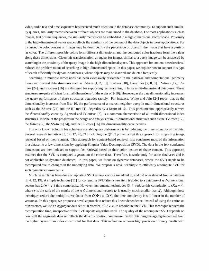
Figure 4. A 1-dimensional index structure for the 2-dimensional data items� � � �� and � .

The index structure is constructed using the coordinates of the data items along axis � � .

This technique works well for static databases. However, in dynamic databases, where inserts and deletes occur

frequently in the database, the axes may have to be reoriented to cope with these frequent updates to the database.

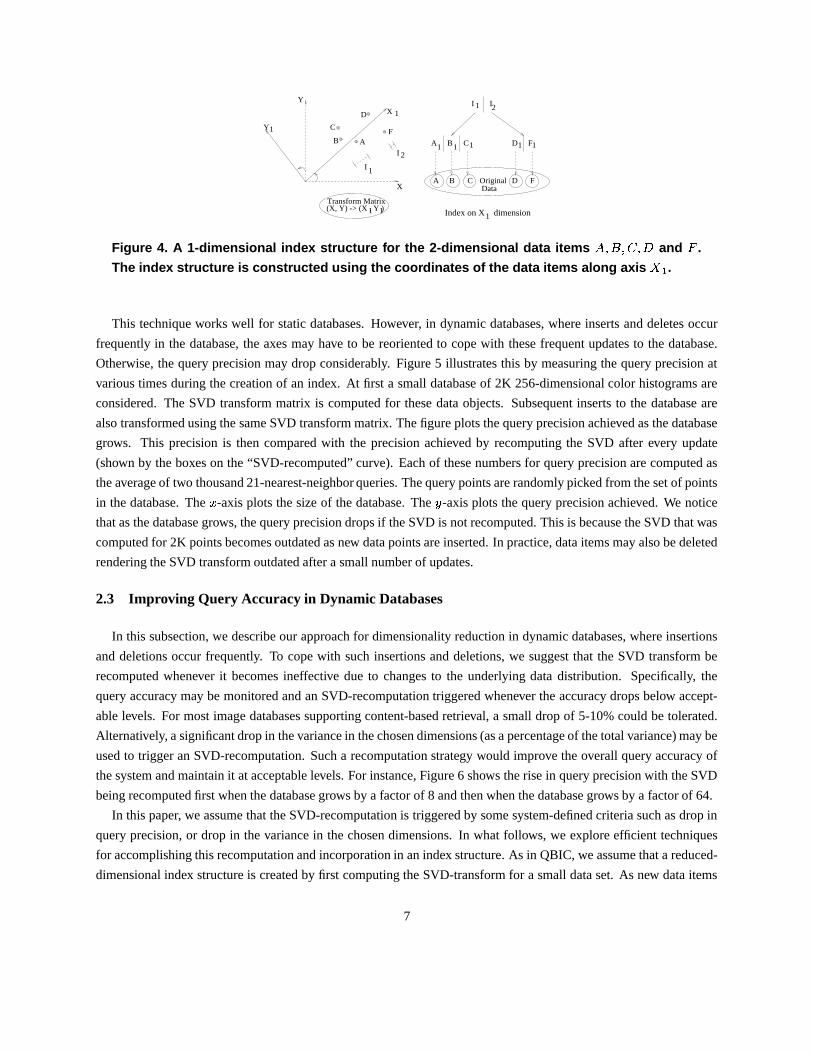
Otherwise, the query precision may drop considerably. Figure 5 illustrates this by measuring the query precision at

various times during the creation of an index. At first a small database of 2K 256-dimensional color histograms are

considered. The SVD transform matrix is computed for these data objects. Subsequent inserts to the database are

also transformed using the same SVD transform matrix. The figure plots the query precision achieved as the database

grows. This precision is then compared with the precision achieved by recomputing the SVD after every update

(shown by the boxes on the “SVD-recomputed” curve). Each of these numbers for query precision are computed as

the average of two thousand 21-nearest-neighbor queries. The query points are randomly picked from the set of points

in the database. The � -axis plots the size of the database. The � -axis plots the query precision achieved. We notice

that as the database grows, the query precision drops if the SVD is not recomputed. This is because the SVD that was

computed for 2K points becomes outdated as new data points are inserted. In practice, data items may also be deleted

rendering the SVD transform outdated after a small number of updates.

2.3 Improving Query Accuracy in Dynamic Databases

In this subsection, we describe our approach for dimensionality reduction in dynamic databases, where insertions

and deletions occur frequently. To cope with such insertions and deletions, we suggest that the SVD transform be

recomputed whenever it becomes ineffective due to changes to the underlying data distribution. Specifically, the

query accuracy may be monitored and an SVD-recomputation triggered whenever the accuracy drops below accept-

able levels. For most image databases supporting content-based retrieval, a small drop of 5-10% could be tolerated.

Alternatively, a significant drop in the variance in the chosen dimensions (as a percentage of the total variance) may be

used to trigger an SVD-recomputation. Such a recomputation strategy would improve the overall query accuracy of

the system and maintain it at acceptable levels. For instance, Figure 6 shows the rise in query precision with the SVD

being recomputed first when the database grows by a factor of 8 and then when the database grows by a factor of 64.

In this paper, we assume that the SVD-recomputation is triggered by some system-defined criteria such as drop in

query precision, or drop in the variance in the chosen dimensions. In what follows, we explore efficient techniques

for accomplishing this recomputation and incorporation in an index structure. As in QBIC, we assume that a reduced-

dimensional index structure is created by first computing the SVD-transform for a small data set. As new data items

7

45

50

55

60

65

70

75

80

85

2 4 8 16 32 64 128 256

Pre

cisi

on fo

r A

21-

Nea

rest

-Nei

ghbo

r Q

uery

Database Size (in thousands of points)

SVD computed only at 2KSVD recomputed

Figure 5. Drop in query precision for a 21-nearest-neighbor query with the growth of a 256-

dimensional color histogram database: Total size is 144K. Reduced-dimensionality is 32. Boxes

indicate where recomputation is done for “SVD-recomputed" curve.

are inserted and old ones deleted, the SVD-transform (basis matrix) has to be first recomputed, and then incorporated

in the index structure.

3 Recomputing SVD Transform Matrix

In this section, we describe how to recompute the SVD-transform in a dynamic index. We assume the index stores

all data items at the leaf level. We consider two principal approaches for computing the SVD transform matrix. The

first approach uses the entire data to determine this matrix. The second approach uses an aggregate data set which is

much smaller than the original database to reduce computation overheads.

3.1 SVD Recomputation using Entire Data

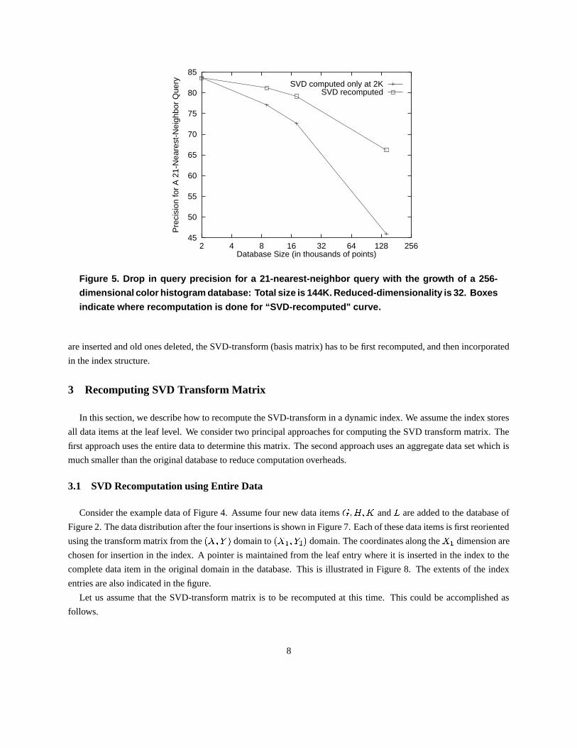
Consider the example data of Figure 4. Assume four new data items� �� and � are added to the database of

Figure 2. The data distribution after the four insertions is shown in Figure 7. Each of these data items is first reoriented

using the transform matrix from the � � �� domain to � � � � � � � domain. The coordinates along the �� dimension are

chosen for insertion in the index. A pointer is maintained from the leaf entry where it is inserted in the index to the

complete data item in the original domain in the database. This is illustrated in Figure 8. The extents of the index

entries are also indicated in the figure.

Let us assume that the SVD-transform matrix is to be recomputed at this time. This could be accomplished as

follows.

8

50

55

60

65

70

75

80

85

2 4 8 16 32 64 128 256

Pre

cisi

on fo

r A

21-

Nea

rest

-Nei

ghbo

r Q

uery

Size of the database (in thousands of points)

SVD

Figure 6. Improvement in query precision of Figure 5 due to SVD-recomputation: Recomputa-

tion occurs when the database size is 18K and 144K.

C

Y

X

G

1Y

D

B

1

H

LK

F

X

A

Figure 7. Data after adding 4 new items� �� and � .

Step 1 (Data Access): Access all the data objects� � � � �� and � through the leaves of the index.

Step 2 (SVD Computation): Determine the SVD-transformation matrix for the data items.

Since the transform has to be computed over the entire dataset, we refer to this technique as the All-Data-SVD, or

simply as the SVD technique, where there is no ambiguity. Since the time overhead for computing SVD in step 2 is

directly proportional to the number of points used in the computation, the overhead is quite large for large datasets and

dominates the total overhead.

3.2 SVD Recomputation using Aggregate Data

In order to reduce the time for SVD computation, we use an aggregate data set whose size is much smaller than

the size of the database. The aggregation is performed based on the structure of the existing index. This allows us to

9

1H1G1

A B C G

1Transform Matrix

1

H

TT

(X, Y) -> (X , Y )

X

Y

3

4

I 2

I

I

A KB

Index on X dimension1

HG

F

L

D

1

C

1

Y1

I

XX 1

Y1

C

LK

K1 L1

I42I

1 F1

D F

DA1 B1

Original Data

2J1J

3I 1 I

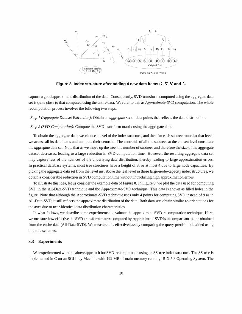
Figure 8. Index structure after adding 4 new data items� �� and � .

capture a good approximate distribution of the data. Consequently, SVD-transform computed using the aggregate data

set is quite close to that computed using the entire data. We refer to this as Approximate-SVD computation. The whole

recomputation process involves the following two steps.

Step 1 (Aggregate Dataset Extraction): Obtain an aggregate set of data points that reflects the data distribution.

Step 2 (SVD-Computation): Compute the SVD-transform matrix using the aggregate data.

To obtain the aggregate data, we choose a level of the index structure, and then for each subtree rooted at that level,

we access all its data items and compute their centroid. The centroids of all the subtrees at the chosen level constitute

the aggregate data set. Note that as we move up the tree, the number of subtrees and therefore the size of the aggregate

dataset decreases, leading to a large reduction in SVD-computation time. However, the resulting aggregate data set

may capture less of the nuances of the underlying data distribution, thereby leading to large approximation errors.

In practical database systems, most tree structures have a height of 3, or at most 4 due to large node capacities. By

picking the aggregate data set from the level just above the leaf level in these large-node-capacity index structures, we

obtain a considerable reduction in SVD computation time without introducing high approximation errors.

To illustrate this idea, let us consider the example data of Figure 8. In Figure 9, we plot the data used for computing

SVD in the All-Data-SVD technique and the Approximate-SVD technique. This data is shown as filled holes in the

figure. Note that although the Approximate-SVD technique uses only 4 points for computing SVD instead of 9 as in

All-Data-SVD, it still reflects the approximate distribution of the data. Both data sets obtain similar re-orientations for

the axes due to near-identical data distribution characteristics.

In what follows, we describe some experiments to evaluate the approximate SVD-recomputation technique. Here,

we measure how effective the SVD-transform matrix computed by Approximate-SVD is in comparison to one obtained

from the entire data (All-Data-SVD). We measure this effectiveness by comparing the query precision obtained using

both the schemes.

3.3 Experiments

We experimented with the above approach for SVD-recomputation using an SS-tree index structure. The SS-tree is

implemented in C on an SGI Indy Machine with 192 MB of main memory running IRIX 5.3 Operating System. The

10

(b) Approximate-SVD

FK

L

B

(a) All-Data-SVD

D

A

GH

C

KL

H

BF

A

G

D

C

Figure 9. Data samples used in computing SVD: Black dots indicate points used in the compu-

tation.

page size of the SS-tree is fixed at 8K. The capacity of the SS-trees, therefore, depended on the number of dimensions

being indexed. For instance, for 12-dimensions, the node capacity was 120 whereas for 32-dimensions the capacity

was 55. The re-insertion parameter of the SS-tree is set to 30% of the node capacity and the minimum capacity to

40% of the node capacity. These are the same as in other implementations of SS-trees [24] and R*-trees [1]. To

simulate real-database scenarios, only 25% nodes of an index are cached in memory in all our experiments. The

caching strategy is simple and ensured that all the non-leaf nodes are in memory along with first few leaf nodes that

are created.

We evaluate the effectiveness of the approximate computation of the SVD on two real image databases and one

synthetic dataset. The first real image dataset is the Corel Image Collection, which consists of 26K 48-dimensional

feature vectors representing image textures. The second one is an assortment of 18K 256-dimensional color histograms

obtained from the WWW.

For each database, we first compute the SVD-transform for a fraction (1/8��

) of the database, reduce the dimension-

ality and then construct an index for the reduced-dimensional data. We then insert the remaining points of the database

into the index. Then, we recompute the SVD-transforms using both aggregate data (as in Approximate-SVD) and the

entire data (as in All-Data-SVD). The computation times for determining the transform are measured. The quality of

the transforms is compared by evaluating the average query precision for 2000 nearest-neighbor queries. The query

points are randomly chosen from among the data points in the database. In what follows, we describe the results for

the two databases.

3.3.1 Texture Dataset

For the texture database, we assume that the SVD-transform is computed when the database has approximately 3K

data items (corresponding to��

of the total database size of 26K). We then insert 23K more data points into this

index and then determine the SVD-transform matrix using Approximate-SVD and All-Data-SVD techniques. We

measure the average query precision achieved when the resulting SVD-transform matrices are applied to the original

48-dimensional data.

First, we examine the computation times of the two techniques. We note that the cost of obtaining the aggregate data

in Approximate-SVD is the same as that of All-Data-SVD. Since this cost is very small (15 seconds) in comparison to

the SVD-computation times, we only compare the SVD-computation times for the two techniques. Table 1 shows these

computation times. Note that as we increase the number of dimensions, the capacity of the index nodes decreases.

11

Consequently, the ratio of the aggregate data set to that of the database also increases since the aggregate data set is

obtained from the parents of leaf nodes in an index. This leads to an increase in the SVD computation time for the

Approximate-SVD. However, the computation time is still smaller by around two orders of magnitude than the time

for computing using the entire data set.

Dimensions Approximate-SVD SVD

Points Time (s) Points Time (s)

8 205 1.6 26K 209

12 272 2.1 26K 209

16 333 2.65 26K 209

20 403 3.1 26K 209

Table 1. SVD-computation times using Approximate-SVD and All-Data-SVD (SVD) techniques.

Database: 26K 48-dimensional texture vectors.

Next, we evaluate the query precision achieved using the approximate technique. Figures 10 and 11 show the

average precisions for nearest-neighbor queries using the transform matrices computed by the All-Data-SVD and

Approximate-SVD techniques. Figure 10 plots the query precision for different number of nearest neighbors assuming

a reduced dimensionality of 12. Figure 11 plots the query precision for a varying number of reduced dimensions

and 21-nearest-neighbor queries. We observe that Approximate-SVD achieves nearly the same query precision as

SVD. This is significant given the efficiency of computing Approximate-SVD as opposed to SVD. In contrast, other

techniques such as DFT (also plotted) do not achieve as high a precision.

64

66

68

70

72

74

76

78

80

82

84

20 25 30 35 40 45 50 55

Que

ry P

reci

sion

usi

ng 1

2 R

educ

ed D

imen

sion

s

Number of Neighbors Requested

SVDApproximate-SVD

VDFT

Figure 10. Precision of nearest-neighbor queries on 26K 48-dimensional texture vectors: Vary-

ing number of neighbors requested for 12 dimensions.

12

50

55

60

65

70

75

80

85

90

8 10 12 14 16 18 20

Pre

cisi

on fo

r A

21-

Nea

rest

-Nei

ghbo

r Q

uery


SVDApproximate-SVD

VDFT

Figure 11. Precision of nearest-neighbor queries on 26K 48-dimensional texture vectors: Vary-

ing number of chosen dimensions for 21-nearest-neighbor queries.

3.3.2 Color Dataset

For the color database, we assume that the SVD-transform is computed when the database has 2K entries (correspond-

ing again to��

of the database size), and add another 16K entries using this transform. The SVD-transform is

recomputed using both Approximate-SVD and All-Data-SVD techniques. As before, we compared the relative merits

of the two techniques by examining the computation time and query precision achieved.

Table 2 shows the computation times for Approximate-SVD and All-Data-SVD. As the dimensionality of the index

increases from 16 to 64, the node capacity decreases. This leads to an increase in the size of the aggregate dataset

(because of the increase in the number of subtrees at the lowest non-leaf level), thereby leading to an increasing in

SVD-computation times. We observe that the computation time for Approximate-SVD is less by a factor of 25 than

that of All-Data-SVD.

Dimensions Approximate-SVD SVD

Points Time (s) Points Time (s)

16 236 55 18K 5013

32 416 102 18K 5013

48 632 154 18K 5013

64 821 201 18K 5013

Table 2. SVD-computation times using Approximate-SVD and All-Data-SVD (SVD) techniques.

Database: 18K 256-dimensional color histograms.

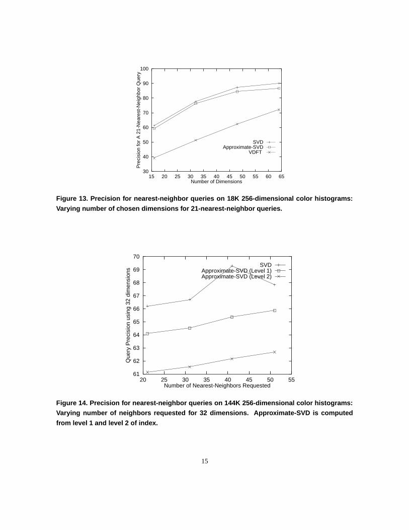
Figures 12 and 13 plot the query precision obtained for this dataset. As before, we consider a varying number of

13

nearest neighbors as well as a varying number of reduced dimensions. The results are similar to those for the Texture

dataset. Once again we observe that the query precision using Approximate-SVD is within 5% of the query precision

using SVD, and that the query precision using DFT (VDFT) is much lower.

50

55

60

65

70

75

80

20 25 30 35 40 45 50 55

Que

ry P

reci

sion

usi

ng 3

2 di

men

sion

s

Number of Nearest-Neighbors Requested

SVDApproximate-SVD

VDFT

Figure 12. Precision for nearest-neighbor queries on 18K 256-dimensional color histograms:

Varying number of neighbors requested for 32 dimensions.

Experiments with Aggregation from different levels of index

In the above experiments, we evaluated the quality of approximate-SVD assuming the aggregate data is obtained

from the level just above the leaves. Next, we examine the impact of obtaining aggregate data from higher levels of

the index on the quality of approximate-SVD. We examine two levels of the index one just above the index (level 1),

and another just two levels above the leaves (level 2). Using the aggregate data at each of these levels, we compute

the approximate-SVD transform and compare their query precision. We conduct these experiments on a 144K 256-

dimensional color histogram database, whose SVD is first computed when the database has only 18K histograms.

Figure 14 illustrates the query precision for 32 reduced dimensions. We observe that as we move up the tree

for obtaining the aggregate data, the query precision drops. This is expected as the nuances in the underlying data

distribution are lost as we move to higher levels of an index structure. Similar results are also obtained in figure 15

where the number of reduced dimensions is varied from 16 to 64.

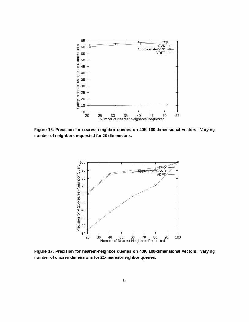
3.4 Experiments with a synthetic dataset

Next we describe our experiments on a synthetic dataset. The dataset is generated as follows. The dimensionality

of the dataset is chosen to be 100. Initially, 5K data points are generated so that the variance is nearly the same in all

the dimensions: for each dimension, the range of the domain is fixed as [0,1] and data values are randomly generated

14

30

40

50

60

70

80

90

100

15 20 25 30 35 40 45 50 55 60 65

Pre

cisi

on fo

r A

21-

Nea

rest

-Nei

ghbo

r Q

uery


SVDApproximate-SVD

VDFT


Varying number of chosen dimensions for 21-nearest-neighbor queries.

61

62

63

64

65

66

67

68

69

70

20 25 30 35 40 45 50 55

Que

ry P

reci

sion

usi

ng 3

2 di

men

sion

s


SVDApproximate-SVD (Level 1)Approximate-SVD (Level 2)


Varying number of neighbors requested for 32 dimensions. Approximate-SVD is computed

from level 1 and level 2 of index.

15

40

50

60

70

80

90

100

0 50 100 150 200 250 300

Pre

cisi

on fo

r A

21-

Nea

rest

-Nei

ghbo

r Q

uery


SVDApproximate-SVD (Level 1)Approximate-SVD (Level 2)


Varying number of chosen dimensions for 21-nearest-neighbor queries. Approximate-SVD is

computed from level 1 and level 2 of index.

in this range. We then increase the database size to 40K (as in the previous experiments) by adding 35K more points.

For these 35K points, the variance is decreased by half for every 20 dimensions: the points in the first 20 dimensions

range over the domain [0,1], those in the next 20 dimensions range over [0, 0.5], and so on.

Given this synthetic dataset, the SVD transform in computed for the first 5K data points. A reduced-dimensional

index is constructed using the first 20 dimensions after this data transformation. Subsequently, the remaining 35K

points are then inserted in the index. The SVD-transform is recomputed using the index. As in the previous cases,

approximate computation of SVD using the index is upto two orders of magnitude faster than computation using entire

data. Figures `16 and 17 describe the quality of approximate-SVD transform in comparison to SVD and DFT. These

results indicate that the query precision achieved by approximate-SVD is comparable to that of SVD. Note that DFT

achieves poor query precision for the same synthetic dataset.

In these experiments, we have observed that computing approximate-SVD using aggregate data from an exist-

ing reduced-dimensional index achieves good query precision while requiring low computation overheads. The

approximate-SVD may, however, perform poorly if the clusters of the index do not reflect the underlying distribution.

This may happen due to a poor choice of the dimensions for the reduced-dimensional index based on initial database

characteristics. In such a case, the index may be reconstructed using the current “most-varying” set of dimensions,

and then the clusters from this index may be used for computing approximate-SVD transform.

16

10

15

20

25

30

35

40

45

50

55

60

65

20 25 30 35 40 45 50 55

Que

ry P

reci

sion

usi

ng 2

0/10

0 di

men

sion

s


SVDApproximate-SVD

VDFT

Figure 16. Precision for nearest-neighbor queries on 40K 100-dimensional vectors: Varying

number of neighbors requested for 20 dimensions.

10

20

30

40

50

60

70

80

90

100

20 30 40 50 60 70 80 90 100

Pre

cisi

on fo

r A

21-

Nea

rest

-Nei

ghbo

r Q

uery


SVDApproximate-SVD

VDFT

Figure 17. Precision for nearest-neighbor queries on 40K 100-dimensional vectors: Varying

number of chosen dimensions for 21-nearest-neighbor queries.

17

4 Incorporating Recomputed SVD-transform in Reduced-Dimensional Index

In the previous section, we examined how to determine the SVD-transform matrix during recomputation. In this

section, we explore how to incorporate the transform matrix in the existing reduced-dimensional index structure.

Incorporating the recomputed SVD transform at the leaf level entries is relatively straightforward: just apply the

new transform individually to each data item and store the reduced dimensions in the leaf level entries of the in-

dex. Incorporation is much more complex for the index entries, since this has a direct impact on subsequent query

performance. We discuss below two obvious approaches to this incorporation. The first, called Tree-Reconstruct or

simply as Reconstruct, reconstructs the entire index afresh. The second approach, called Structure-Reuse or simply as

Reuse, reuses the existing index structure and adjusts the extents of the index entries without any structural changes.

Finally, we detail our approach that combines the benefits of the two previous approaches. This scheme called Reuse-

Reconstruct performed much better in our experiments.

The Reconstruct strategy reconstructs the entire index from the data entries. If the data can reside entirely in

memory, this reconstruction can be accomplished efficiently using the techniques of in-memory index structures such

as k-d trees and its variants [15, 10, 23]. For disk-resident datasets (like what we used in our experiments), the

reconstruction has to be done a few data items at a time, leading to high insertion costs. On the positive side, this

technique achieves a good query response time since the index structure reflects the data distribution accurately.

The Structure-Reuse strategy reuses the existing index structure and recomputes the extent of the index entries

without making any structural changes. The extent of an index entry is recomputed recursively using the extents of

the child entries. These updates are carried out in a bottom-up manner starting with the leaf level. Since no structural

changes are made, this incorporation strategy is quite efficient. However, the extents of the index entries are likely to

increase due to reorientation of the SVD axes. As a result, query performance degrades. In what follows, we describe

a third scheme that combines the fast query response times of a tree-reconstruction strategy and the low incorporation

overheads of a structure-reuse strategy. Note that all three schemes have the same query precision, since they use the

same SVD matrix for transforming the data items.

4.1 The Reconstruct-Reuse Approach

This approach for incorporation selectively reconstructs subtrees in the index and reuses the higher levels of the

index. Figure 18 depicts this strategy for an arbitrary index. Based on the available memory resources, a specific level

of the index is chosen for reconstruction. Above this chosen level, the index structure is reused as in the Structure-

Reuse strategy, and below this level the index is recomputed as in the Reconstruct strategy. Choosing a level close to

the root leads to more memory requirements since a larger subtree of the index has to be manipulated in the memory.

The reconstruction of a subtree is performed using the VAMSplit technique [23]. The set of data items in the subtree

is partitioned recursively until each sub-partition fits in a single node (disk page). The partitioning is accomplished by

determining the most varying dimension, and splitting the data along an appropriate place in this dimension. Given �data items to be partitioned into two sub-partitions, the number of data items in the first sub-partition, � , is computed

based on a node capacity of�

as follows.

� &��

��

18

Chosen Level Index

Reuse

Reconstruct

Incorporation Strategy

Figure 18. Reuse-Reconstruct Strategy for Incorporating SVD-transform in an Existing Index

White et al. [23] showed that this choice of � minimizes the number of nodes in the created index. They also showed

that the resulting index supports fast queries.

The query performance of the Reuse-Reconstruct strategy described above is enhanced by selectively deleting some

data entries during subtree reconstruction and reinserting them in the entire tree. This eliminates the impact of data

entries that are misfits in a subtree after the transform matrix is applied. An entry is considered to be a misfit in a subtree

if its deletion results in a considerable decrease in the volume. We found that this selective re-insertion improved the

query performance.

4.2 Experimental comparison of the three approaches

We experimented with the above incorporation strategies on an image database of 26K 48-dimensional texture

vectors. These strategies are used to incorporate a recomputed SVD-transform matrix in an existing SS-tree index for

the texture data. We evaluated the incorporation strategies by measuring incorporation times and query response times

after incorporation. The query response times are computed as the average over two thousand 21-nearest-neighbor

queries. Each query is generated using a randomly picked data point from the database.

For the Reuse-Reconstruct scheme, we used selective reinserts. We assumed that only those data entries that resulted

in a 50% radius decrease for a subtree are considered for deletion. The number of such reinserted entries is further

limited to 5% of the entries in a subtree. For the Reconstruct scheme, we assumed the tree is reconstructed using an

SS-tree [24]. In all the experiments, we assumed that only 25% of the index nodes are cached in memory.

Scheme Incorporation Query time

time (s) (ms, disk I/O)

Reconstruct 1363 (27, 154)

Reuse 22 (52, 275)

Reuse-Reconstruct 42 (30, 160)

Table 3. Incorporation and 21-nearest-neighbor query response times for different schemes.

Database: 26K 48-dimensional texture vectors. Reduced dimensionality: 12.

Table 3 compares the three incorporation schemes for the texture database. The best query response time is achieved

by reconstructing the entire index as in the Reconstruct scheme. However, this scheme has a high incorporation cost.

19

On the other hand, the best incorporation time is obtained by reusing the existing structure as in the Reuse scheme.

However, this scheme lead to a considerable increase in the extents of index entries. The average radius of the index

entries actually tripled in this case. Consequently, the query response times nearly doubled. These two schemes

form the two extremes. In comparison, the Reuse-Reconstruct scheme achieves a query response time that is within

10% of the best query response time registered (by the Reconstruct scheme). The incorporation time of the Reuse-

Reconstruct scheme is double that of the Reuse scheme, though within acceptable limits and much lower than that of

the Reconstruct scheme. The performance advantages of the Reuse-Reconstruct scheme are expected to be substantial

even if other strategies are used for tree-reconstruction.

16

32

64

128

256

512

1024

2048

8 10 12 14 16 18 20

Inco

rpor

atio

n T

ime

(s)


ReuseReuse-Reconstruct

Reconstruct

Figure 19. Incorporation times for differet incorporation schemes as number of chosen dimen-

sion is varied. Database: 26K 48-dimensional texture vectors.

Figures 19 and 20 elaborate these results for incorporation and query response times when the number of reduced

dimensions is varied. The results are similar to the case of 12 dimensions in Table 3. Similar results were also obtained

for color histograms. These results indicate that our proposed scheme, which combines low incorporation times of

the Reuse scheme and the low query response time of the Reconstruct scheme, is a viable strategy for incorporating

recomputed SVD transforms in dynamic databases.

5 Conclusions

Performance of similarity searching in high dimensional index structures degrades as the dimensionality of the

data increases. Dimensionality reduction is the only known solution to support fast searching. Such dimensionality

reduction is accompanied by a loss of information and a consequent loss in query accuracy. This loss is minimized if

the data is first transformed using an SVD transform, which concentrates most of the information in a few dimensions.

The reduced-dimensionality data obtained from an SVD-transformation could then be used to support fast searching

with high query accuracy. Current systems using this approach perform a static transformation of the data. In this

paper, we illustrate why such an approach may lead to degradation in query accuracy as data items are inserted and

20

100

150

200

250

300

350

400

8 10 12 14 16 18 20

Que

ry R

espo

nse

Tim

e (in

dis

k ac

cess

es)


ReuseReuse-Reconstruct

Reconstruct

Figure 20. Query response times for different incorporation schemes as number of chosen

dimensions is varied. Database: 26K 48-dimensional texture vectors.

Transform Query Query Accumulated Accumulated

Comp. + Precision time SVD-time (s) Incorporation

Incorporation (disk I/O) time (s)

Approximate-SVD + 61.6 1390 916 184

Reuse-Reconstruct

SVD + Reconstruct 66.2 1270 40318 21370

Table 4. SVD-transform computation and incorporation times for 2 recomputations during in-

sertion of 144K 256-dimensional color histograms. Query response time and query precision

after the insertion process are also indicated.

deleted. We, therefore, propose novel techniques to cope up with the updates to the database.

First, we propose an efficient techniques for approximately computing SVD. In contrast to existing techniques, our

technique uses a small aggregate dataset instead of the entire data to compute the SVD transform. Since the size of the

aggregate dataset is quite small in comparison to that of the database, the overheads of computation are reduced by up

to two orders of magnitude. The aggregate data is obtained from the index clusters and closely reflects the underlying

data distribution. This results in approximation error of less than 5%.

We then explored how to efficiently incorporate the recomputed SVD-transform in the existing reduced-dimensional

index structure. Straightforward approaches to incorporation of the transform in an index could degrade index quality

and increase subsequent query response times. Therefore, we examined different ways to efficiently incorporate the

transform matrix in the index without degrading query performance. We proposed a novel strategy that selectively

reconstructs subtrees at a chosen level and reuses the index at higher levels. The level of reconstruction can be chosen

to suit available memory resources.

21

We also ran experiments to measure the impact of multiple cycles of SVD recomputation and subsequent incorpo-

ration in an existing index. The experiments were conducted for 144K 256-dimensional color histograms. An initial

All-Data-SVD was computed and an SS-tree index was constructed for 3K data items. Two recompute-incorporate

instances were chosen at database sizes of 18K and 144K. The results comparing our techniques with existing ones

are shown in Table 4. The total times for the SVD recomputations and subsequent incorporations, in addition to query

precision and query response time are indicated in the table.

Note that the query precision using Approximate-SVD is within 9% of the precision using All-Data-SVD. The

response time is also close to that of a completely reconstructed index. However, the reduction in SVD-computation

time and incorporation times are around two orders of magnitude for our proposed techniques. We conclude that

such huge reduction in computation overheads will contribute to high index performance both in single-user and

concurrent systems. These experiments considered dynamic environments in which the size of the database grows by

large amounts through insert operations. Similar shifts in SVD vectors can also be caused by a smaller number of

updates (that include deletes). In a realistic setting, we expect that recomputation of SVD would be triggered either

after a predetermined number of update operations, or by a loss in query precision. In future, we will investigate the

robustness of our approach in the context of other types of queries such as epsilon queries, and other datasets.

References

[1] N. Beckmann, H. Kriegel, R. Schneider, and B. Seeger. The R* tree: An efficient and robust access method for points and

rectangles. Proc. of the ACM SIGMOD Intl. Conf. on Management of Data, pages 322–331, May 23-25 1990.

[2] S. Berchtold, D. A. Keim, and H. P. Kreigel. The X-tree: An index structure for high dimensional data. Proceedings of the

Int. Conf. on Very Large Data Bases, 1996.

[3] S. Chandrasekharan, B. S. Manjunath, Y. F. Wang, J. Winkeler, and H. Zhang. An eigenspace update algorithm for image

analysis. CVGIP: Journal of graphical Models and image processing, 1997.

[4] R. Degroat and R. Roberts. Efficient numerically stabilized rank-one eigenstructure updating. IEEE transactions on acoustic

and signal processing (T-ASSP), 38(2):301–316, 1990.

[5] C. Faloutsos and K. Lin. Fastmap: A fast algorithm for indexing, data-mining and visualization of traditional and multimedia

datasets. Technical Report CS-TR-3383, Univ. of Maryland Institute for Advanced Computer Studies, Jan. 1994.

[6] C. Faloutsos, M. Ranganathan, and Y. Manolopoulos. Fast subsequence matching in time-series databases. In Proc. ACM

SIGMOD Int. Conf. on Management of Data, pages 419–429, Minneapolis, May 1994.

[7] M. W. Freeston. The bang file: a new kind of grid file. Proc. of the ACM SIGMOD Intl. Conf. on Management of Data, pages

260–269, May 1987.

[8] M. W. Freeston. A general solution of the n-dimensional B-tree problem. Proc. of the ACM SIGMOD Intl. Conf. on Manage-

ment of Data, May 1995.

[9] M. W. Freeston. A new generic index technology. Proc. NASA Goddard Conf. on Mass Storage Technologies, September

1996.

[10] J. H. Friedman, J. Bentley, and R. Finkel. An algorithm for finding best matches in logarithmic expected time. ACM

transactions on mathematical software, 3(3):209–226, 1977.

[11] G. H. Golub and C. F. van Loan. Matrix Computations. The John Hopkins Press, 1989.

[12] M. Gu and S. C. Eisenstat. A stable and fast algorithm for updating the singular value decomposition. Technical Report

YALEU/DCS/RR-966, Yale University, New Haven, CT, 1994.

22

[13] A. Guttman. R-trees: A dynamic index structure for spatial searching. Proc. ACM SIGMOD Int. Conf. on Management of

Data, pages 47–57, 1984.

[14] D. Hull. Improving text retrieval for the routing problem using latent semantic indexing. In Proc. of the 17th ACM-SIGIR

Conference, pages 282–291, 1994.

[15] J.L.Bentley. Multi-dimensional binary search trees used for associative searching. Communications of the ACM, 18:509–517,

1975.

[16] N. Katayama and S. Satoh. The SR-tree: An index structure for high-dimensional nearest-neighbor queries. Proc. ACM

SIGMOD Int. Conf. on Management of Data, pages 369–380, May 1997.

[17] K.-I. Lin, H. V. Jagdish, and C. Faloutsos. The TV-tree: An index structure for high-dimensional data. VLDB Journal,

3:517–542, 1994.

[18] D. B. Lomet and B. Salzberg. The hB-tree: A multi-attribute indexing method with good guaranteed performance. Proc.

ACM Symp. on Transactions of Database Systems, 15(4):625–658, December 1990.

[19] G. Mathew, V. U. Reddy, and S. Dasgupta. Adaptive estimation of eigenspaces. IEEE Transactions in Signal Processing,

43(2):401–411, 1995.

[20] R. Ng and A. Sedighian. Evaluating multi-dimensional indexing structures for images transformed by principle component

analysis. Proc. of the SPIE, 2670:50–61, 1994.

[21] W. Niblack, R. Barber, W. Equitz, M. Flickner, E. Glasman, D. Petkovic, and P. Yanker. The QBIC project: Querying images

by content using color, texture and shape. In Proc. of the SPIE Conf. 1908 on Storage and Retrieval for Image and Video

Databases, volume 1908, pages 173–187, Feb. 1993.

[22] G. Salton. Automatic Text Processing. Addison-Wesley, 1989.

[23] D. White and R. Jain. Algorithms and strategies for similarity retrieval. Proc. of the SPIE Conference, 1996.

[24] D. White and R. Jain. Similarity indexing with the SS-tree. Proc. Int. Conf. on Data Engineering, pages 516–523, 1996.

[25] D. Wu, D. Agrawal, A. El Abbadi, A. Singh, and T. R. Smith. Efficient retrieval for browsing large image databases. Proc.

Conf. on Information and Knowledge Management, pages 11–18, Nov. 1996.

23

dimensionality reduction for similarity searching … reduction for similarity searching in dynamic...

Documents