direct measurement of mercury reactions … library/research/coal/ewr/air-quality...direct...

EPRI • 3420 Hillview Avenue, Palo Alto, California 94304-1395 • Palo Alto, California 94303 • USA800.313.3774 • 650.855.2121 • [email protected] • www.epri.com

DIRECT MEASUREMENT OF MERCURYREACTIONS IN COAL POWER PLANT PLUMES

Final Technical Report, March 2006

Prepared for:

AAD Document Control

U.S. Department of Energy National Energy Technology Laboratory PO Box 10940, MS 921-107 Pittsburgh, PA15236-0940

DOE Award DE-FC26-03NT41724Performance Monitor: William Aljoe

Cosponsor(s)

National Energy Technology LaboratoryU.S. Department of EnergyPittsburgh, PA

Wisconsin Focus on EnergyMadison, WI

Electric Power Research InstitutePalo Alto, CA

Prepared by

Leonard Levin

Electric Power Research Institute3412 Hillview Ave.

Palo Alto, California 94303

March 2006

DISCLAIMER OF WARRANTIES AND LIMITATION OF LIABILITIES

THIS DOCUMENT WAS PREPARED BY THE ORGANIZATION(S) NAMED BELOW AS AN ACCOUNT OF WORKSPONSORED OR COSPONSORED BY THE ELECTRIC POWER RESEARCH INSTITUTE, INC. (EPRI).NEITHER EPRI, ANY MEMBER OF EPRI, ANY COSPONSOR, THE ORGANIZATION(S) BELOW, NOR ANYPERSON ACTING ON BEHALF OF ANY OF THEM:

(A) MAKES ANY WARRANTY OR REPRESENTATION WHATSOEVER, EXPRESS OR IMPLIED, (I) WITHRESPECT TO THE USE OF ANY INFORMATION, APPARATUS, METHOD, PROCESS, OR SIMILAR ITEMDISCLOSED IN THIS DOCUMENT, INCLUDING MERCHANTABILITY AND FITNESS FOR A PARTICULARPURPOSE, OR (II) THAT SUCH USE DOES NOT INFRINGE ON OR INTERFERE WITH PRIVATELY OWNEDRIGHTS, INCLUDING ANY PARTY'S INTELLECTUAL PROPERTY, OR (III) THAT THIS DOCUMENT ISSUITABLE TO ANY PARTICULAR USER'S CIRCUMSTANCE; OR

(B) ASSUMES RESPONSIBILITY FOR ANY DAMAGES OR OTHER LIABILITY WHATSOEVER (INCLUDINGANY CONSEQUENTIAL DAMAGES, EVEN IF EPRI OR ANY EPRI REPRESENTATIVE HAS BEEN ADVISED OFTHE POSSIBILITY OF SUCH DAMAGES) RESULTING FROM YOUR SELECTION OR USE OF THISDOCUMENT OR ANY INFORMATION, APPARATUS, METHOD, PROCESS, OR SIMILAR ITEM DISCLOSED INTHIS DOCUMENT.

ORGANIZATION(S) THAT PREPARED THIS DOCUMENT

Energy & Environmental Research CenterGrand Forks, North Dakota

Electric Power Research InstitutePalo Alto, California

Electric Power Research Institute and EPRI are registered service marks of the Electric Power Research Institute,Inc. EPRI. ELECTRIFY THE WORLD is a service mark of the Electric Power Research Institute, Inc.

Copyright © 2006 Electric Power Research Institute, Inc. All rights reserved.

iii

CITATIONS

This report was prepared by

Energy & Environmental Research Center15 North 23rd StreetGrand Forks, ND 58203

Principal InvestigatorD. Laudal

Electric Power Research Institute3412 Hillview Ave.Palo Alto, CA 94303

Project ManagerL. Levin

This report describes research sponsored by EPRI, the U.S. Department of Energy, and theState of Wisconsin.

The report is a corporate document that should be cited in the literature in the followingmanner:

EPRI, 2006; Mercury Chemistry in Power Plant Plumes; Electric Power Research Institute,Palo Alto, CA.

v

PROJECT DESCRIPTION

Recent field and pilot-scale results indicate that divalent mercury emitted from power plantsmay rapidly transform to elemental mercury within the power plant plumes. Simulations ofmercury chemistry in plumes based on measured rates to date have improved regional modelfits to Mercury Deposition Network wet deposition data for particular years, while notdegrading model verification fits for remaining years of the ensemble. The years with improvedfit are those with simulated deposition in grid cells in the State of Pennsylvania that havematching MDN station data significantly less than the model values.

This project seeks to establish a full-scale data basis for whether or not significant reduction oroxidation reactions occur to mercury emitted from coal-fired power plants, and what numericalredox rate should apply for extension to other sources and for modeling of power plant mercuryplumes locally, regionally, and nationally.

Although in-stack mercury (Hg) speciation measurements are essential to the development ofcontrol technologies and to provide data for input into atmospheric fate and transport models,the determination of speciation in a cooling coal combustion plume is more relevant for use inestimating Hg fate and effects through the atmosphere. It is mercury transformations that mayoccur in the plume that determine the eventual rate and patterns of mercury deposited to theearth’s surface. A necessary first step in developing a supportable approach to modeling anysuch transformations is to directly measure the forms and concentrations of mercury from thestack exit downwind to full dispersion in the atmosphere. As a result, a study was sponsored byEPRI and jointly funded by EPRI, the U.S Department of Energy (DOE), and the WisconsinDepartment of Administration. The study was designed to further our understanding of plumechemistry.

The study was carried out at the We Energies Pleasant Prairie Power Plant, Pleasant Prairie,Wisconsin, just west of Kenosha.

Results & Findings

Aircraft and ground measurements support the occurrence of a reduction in the fraction ofreactive gaseous mercury (RGM) (with a corresponding increase in elemental mercury) as partof the Total Gaseous Mercury (TGM) emitted from the Pleasant Prairie stack. This occurrenceis based on comparison of the RGM concentrations in the plume (at standard conditions)compared to the RGM in the stack. There was found to be a 44% drop in the fraction of RGMbetween the stack exit and the first sampling arc and a 66% reduction from the stack to the 5-mile sampling arc, with no additional drop between the 5- and 10-mile arcs.

vi

Challenges & Objectives

Smaller-scale experiments in both test chambers and pilot-scale coal combustor exhauststreams have indicated the presence of rapid and relatively complete reduction reactionsconverting divalent into elemental mercury within power plant plumes prior to full dispersionin the atmosphere. These measurements, however, have been unable to identify whether thereactions occur during plume rise from physical to virtual stack height (during positive thermalbuoyancy). The presence, rate, completeness, ubiquity, and dependence on sourcecharacteristics of these reactions, however, must be demonstrated in plume environmentsassociated with fully operational power plants. That requirement, to capture either the reactionsor the reaction products of chemistry that may be occurring very close to stack exits in highlyturbulent environments, constrains the precision and reproducibility with which such full-scaleexperiments can be carried out. The work described here is one of several initial steps requiredto test whether, and in what direction, such rapid mercury redox reactions might be occurring insuch plumes.

Applications, Values & Use

The linking of mercury atmospheric sources and downwind receptors, particularly receivingwaters and watersheds with the potential for fish uptake and bioaccumulation of mercury,requires the use of atmospheric physicochemical models, since there is a lack of benignchemical tracers that fully mimic the behavior of mercury in the atmosphere and the biosphere.Current models either inadequately simulate chemical processes in-plume environments, or donot allow such inclusion at all; additionally, there is little direct evidence of what thoseprocesses applicable to mercury might entail. Establishing whether potentially rapid andcomplete mercury redox reactions occur in plume environments, enriched in sulfur and otherco-emitted substances relative to the free atmosphere and not yet fully dispersed into theambient environment, will allow model improvements to better simulate contributions of thosepower plants where such reactions are likely to occur. In turn, this will allow a better fitbetween model outcomes and actual processes in the atmosphere, to allow more realisticallocation of deposited mercury to its sources.

EPRI Perspective

The chemical form of inorganic mercury, whether elemental or divalent, strongly determines itssolubility in precipitable water in the atmosphere. This, in turn, may have orders-of-magnitudeeffects on ground-level concentrations and deposition rates at local and regional scales. Thework done at the Pleasant Prairie Power Plant is a fundamental contribution to understandingthese differences mediated by the trace and major constituents in coal-fired power plant stackplumes. The reactions implied may substantially alter the relative contributions of nearby vs.distant sources to Hg deposition patterns.

Approach

The overall project objective was to gain an understanding of Hg chemistry as a plume movesdownwind from the stack and to determine what changes occur. To accomplish this, aturboprop DHC-6-300 Twin Otter deHavilland Vistaliner aircraft and an automated Tekran

vii

ambient Hg monitor were used. Aircraft sampling was done at three locations downwind of theplume, flying repeated “racetrack” closed loop arcs across the plume at centerline altitude. Thefirst location was approximately 1500 ft downwind of the stack. The second and third locationswere approximately 5 and 10 miles downwind of the stack, respectively.

Determining the altitude and direction of the plume was accomplished using a combination ofvisual inspection (arc closest to the stack) and measurements of NOx concentrations with arapid-response sensor. Except for the closest location, the Tekran Hg analyzer was triggered bya NOx set point.

To establish baseline conditions for comparison with the plume samples, in-stack sampling wascompleted during the flight, providing measurements of the Hg speciation in the stack. Hgsampling at the stack was completed using the Ontario Hydro Hg speciation sampling methodand a continuous mercury monitor. In addition, upwind arcs were flown by the instrumentedaircraft to set levels of incoming RGM and TGM contributions to the plume environment.

Keywords

MercuryUtilitiesPlume(s)Reactive Gaseous MercuryElemental MercuryAir Toxics

ix

ABSTRACT

Studies of mercury sources, source emissions management, and source-receptor relationshipsrely on a knowledge of the chemical forms and amounts of mercury emitted from each source.Models of mercury atmospheric transport and chemistry similarly rely on sourcecharacterization to initiate reactions based on heterogeneous and homogeneousmicroenvironments in the free atmosphere, followed by models of aquatic and terrestrialcycling of the substance.

A key missing element of these simulations, and the data they are based on, is whethersubstantial mercury reactions occur within source emissions plumes to the atmosphere. Theenvironments in these plumes can be expected to be turbulent and contain concentrations of co-emitted material that may be orders of magnitude higher than in the ambient atmosphere. Theseconditions, combined with elevated stack exit temperatures of approximately 200C or more, arefavorable for reactions to occur with mercury under some conditions.

EPRI has conducted two field studies at operating power plants, in 2002 and 2003, toinvestigate the possible reduction or oxidation of mercury under plume conditions. The firststudy was at Plant Bowen, Cartersville, Georgia, operated by Georgia Power, part of SouthernCompany. The second study was at the Pleasant Prairie Power Plant, Pleasant Prairie,Wisconsin, operated by We Energies; there, surface and aircraft measurements were carried outby the University of North Dakota Energy and Environmental Research Center (EERC), withadditional studies at the stack and in plume simulation chambers by Frontier Geosciences. Theprimary focus of this report is on the work at the Pleasant Prairie site.

The overall project objective was to gain an understanding of Hg chemistry as the stackemissions plume is transported downwind from the stack. This was carried out by ground andaircraft measurements conducted simultaneously. Ground measurements characterized mercuryamounts and speciation from the plant boilers through air pollution control devices to the stackbase, and additional measurements via stack ports at about 70% stack height. Aircraftmeasurements were carried out by flying a Twin Otter aircraft through the plume at severallocations (a point nearest the stack, at approximately effective stack height; 5 miles from thestack; and 10 miles from the stack) and measure the speciated Hg composition in the plumeusing an automated ambient Hg monitor.

The results of the project appeared to show a reduction in reactive gas mercury (RGM) (with acorresponding increase in the fraction of elemental Hg) when the proportion of RGM in theplume is compared to the RGM in the stack. There was a 44% reduction of RGM from thestack to the first sample point and a 66% reduction of RGM from the stack to the 5-mile samplepoint, with no additional reduction between the 5- and 10-mile locations.

xi

ACKNOWLEDGMENTS

This work would not have been possible without the efforts of many people. The authors wouldlike to acknowledge the following people.

For their direction and leadership, appreciation is expressed to William Aljoe and LynnBrickett of the U.S. Department of Energy National Energy Technology Laboratory,Pittsburgh. The work could also not have been completed without support from the WisconsinDepartment of Administration, Wisconsin Focus on Energy, and Ingrid Kelley of that program.

At the University of North Dakota, thanks go to Grant Dunham, Blaise Mibek, and RichardSchulz from the Energy & Environmental Research Center and David Delene from the Schoolof Aerospace Sciences,

For Frontier Geosciences, appreciation is extended to Eric Prestbo and his colleagues.

Deep appreciation is also expressed to the other researchers who contributed to the effort,including Ray Valente from the Tennessee Valley Authority.

Special thanks are expressed to Ed Morris and David Michaud of We Energies for facilitatingthe testing conducted at the Pleasant Prairie Power Plant and for all of the help their colleaguesprovided.

xiii

NOMENCLATURE

AF atomic fluorescenceCEM continuous emission monitorCMM continuous mercury monitorCVAFS cold-vapor atomic fluorescence spectroscopyDOE U.S. Department of EnergyEERC Energy & Environmental Research CenterESP electrostatic precipitatorFd value relating gas volume to the heat content of the fuel, equal to dscf/106 BtuGEM gaseous elemental mercuryGPS global positioning systemHCl hydrochloric acidHg mercuryHg0 elemental mercuryHg+2 divalent mercuryHYSPLIT HYbrid Single-Particle Lagrangian Integrated Trajectory modellpm liters per minuteMW megawattsnm nautical mileNOx nitrogen oxidesNOy reactive nitrogen speciesOH Ontario Hydro mercury speciation methodppb parts per billionPRB Powder River BasinRGM reactive gaseous mercurySCR selective catalytic reductionSnCl2 stannous chlorideSO2 sulfur dioxideSPDC static plume dilution chamberTECO Thermal Electron CorporationTVA Tennessee Valley Authority

xv

EXECUTIVE SUMMARY

This report provides a detailed summary of the results obtained for the project entitled “DirectMeasurement of Mercury Reactions in Coal Power Plant Plumes.” The data were obtainedduring testing at the We Energies Pleasant Prairie Power Plant, Pleasant Prairie, Wisconsinduring August-September of 2003. The project was sponsored by EPRI with key funding fromthe U.S. Department of Energy (DOE) National Energy Technology Laboratory and theWisconsin Department of Administration.

Introduction

Characterization of environmental mercury (Hg) and its atmospheric processes, from emissionto deposition, requires both measurement and model simulations for a full understanding.Although in-stack Hg speciation measurements are essential to the development of controltechnologies and to provide data for input into the atmospheric deposition models, thedetermination of speciation in a dispersing power plant stack emissions plume is more relevantfor use in estimating Hg fate and effects after transit through the atmosphere. Mercurytransformations that may occur in plumes determine the rate and the form of Hg transported inthe free atmosphere. Source characterization alone, therefore, will provide an incomplete andperhaps misleading portrayal of the forms of mercury emitted into the atmosphere.

Given these considerations, the Electric Power Research Institute has undertaken a program ofdirect chemical measurements of plume mercury at operating power plants. The first fieldexperiment in this program was at the Plant Bowen (operated by Georgia Power Company),with the Tennessee Valley Authority (TVA) conducting the aircraft studies and the EERC andFrontier Geosciences doing Hg measurements at the stack. The second study was conducted atthe Pleasant Prairie Power Plant, operated by We Energies, with the EERC carrying out boththe aircraft and stack Hg measurements, with additional surface measurements again done byFrontier Geosciences. This report provides insight into the work at Pleasant Prairie; that workwas sponsored by EPRI, EPRI member companies, the U.S. Department of Energy (via theNational Energy Technology Laboratory, Pittsburgh, PA), and the State of WisconsinDepartment of Administration (via Wisconsin Focus on Energy).

Project Objectives

The overall project goal is to gain an understanding of Hg chemistry as a plume movesdownwind from the stack. Specific objectives include:

Develop sampling techniques to measure speciated Hg in the plume. Develop techniques to determine the location of the plume at various points downwind

of the stack. Determine the speciated Hg emissions at the stack and compare these results to those

obtained from the plume sampling.

xvi

Compute a Hg mass balance using dilution factors and other relevant parameters.

Project Description

Power Plant Description

The Pleasant Prairie Power Plant is located near the city of Pleasant Prairie just west ofKenosha, Wisconsin. The Pleasant Prairie plant consists of two units (Units 1 and 2) identicalin operation with the exception of one (Unit 2) having a selective catalytic reduction (SCR)system at the time of the measurements. Each unit has an electrostatic precipitator (ESP) forparticulate control and share a common stack. Specifications of the Pleasant Prairie facility areas follows:

Fuel type: Powder River Basin (PRB) subbituminous coal Boiler capacity: 617 MW (each unit) Boiler type: opposed-fired pulverized coal (both units) NOx control: SCR on Unit 2, low-NOx burners on both units SO2 control: none, combustion of low-sulfur coal (both units) Particulate control: ESP (both units)

The coal is fairly typical of PRB in that both the Hg and chlorine levels in the coal arecomparatively low; the Hg averaged 0.041 µg/g and the chlorine, 10 ppm.

Aircraft and Equipment Used for the Project

The aircraft used for the emission plume sampling was a turboprop DHC-6-300 Twin OtterdeHavilland Vistaliner. The twin-engine plane had a relatively large capacity for equipmentand sufficient onboard electrical supply and could be operated efficiently at low altitudes.These capabilities were accompanied by relatively low fuel consumption at all altitudes. Mostimportantly for the plume study project, it could be flown at relatively slow speeds (80–160 knots/150–300 km/hr) and in tight formation to allow consistent plume traverses at fixedheights and downwind distances.

The Hg analyzer used in the aircraft was a Tekran® Model 2537A mercury vapor analyzercoupled with a Tekran® Model 1130 mercury speciation unit and a Tekran® Model 1135particulate module. The analyzer portion of the system is based on the principle of atomicfluorescence and has detection limits <1 pg/m3. With this system, it was possible tosimultaneously measure elemental mercury (Hg0), reactive gas mercury (RGM), andparticulate-bound Hg species during the flight.

To compare the Hg concentrations in the plume to those in the stack, a dilution factor wasdetermined. Based on the earlier tests conducted at Plant Bowen [2], it was decided that theNOx concentration in the stack vs. that in the plume be used to determine the dilution factor asshown in the following equation:

NOxBackgroundNOxPlume

NOxBackgroundNOxStackRatioDilution

xvii

In addition, the NOx analyzer was used to determine the location of the plume. The analyzerthat was used for this project was a dual range Model 42C Thermo Electron ambient air NOxanalyzer. This analyzer was able to measure 0–50 parts per billion (ppb) NOx in the low rangeand up to 500 ppb NOx in the high range.

Experimental Approach

Aircraft Sampling Locations

Following background sampling at a location upwind of the stack, aircraft sampling was doneat three locations downwind of the plume. The first location was approximately 1500 ft fromthe stack, at approximately the effective stack height. The second and third locations wereapproximately 5 and 10 miles downwind of the stack, respectively. A number of differentpatterns were flown at the closest sampling point in an effort to maximize the sampling timewithin the emissions plume material. At the other two locations, a racetrack pattern was flown.To provide data on aircraft position as a function of time, a satellite-based global positioningsystem was used.

Aircraft sampling flights were conducted in daylight under atmospheric conditions thatpermitted adequate sampling of the stack plume. The weather conditions during the projectfield period were primarily fair weather days with visual flight conditions prevailing. Averagewind speeds were somewhat above this, ranging from 5.3 to 8.3 m/s. These wind speeds werestill low enough that the aircraft was able to locate the plume by NOx sensors, and sometimesvisually.

Stack Sampling

To establish baseline conditions for comparison with the plume samples, in-stack sampling wascarried out simultaneously with the flight, providing measurements of the Hg speciation in thestack. Hg sampling at the stack was completed using the Ontario Hydro (OH) Hg speciationsampling method and a continuous mercury monitor (CMM). Prior to the start of the testing, aCMM was placed at the stack outlet and remained there during the entire project. During eachflight day, one OH sample was taken at the stack.

In addition to Hg measurements by the EERC, the plant operators continuously measured theNOx concentration in the stack using a continuous emission monitor. Although the NOxconcentrations in the stack at the Pleasant Prairie Power Plant were somewhat lower thanoptimal for aircraft plume measurements (since half the flue gas was being treated using anSCR), it was still possible to detect a difference between the background and plume, even at 10miles. The average stack NOx concentration was 144 ppm(v).

Results and Discussion

Stack Results at Pleasant Prairie

The Hg concentrations in the stack were relatively constant during the entire duration of theproject. RGM averaged 34.3% of the total Hg measured. These results were matched very wellby the CMM as shown in Figure ES-1.

xviii

Figure ES-1Plot of the % Hg0 in the Plume Compared to the Stack Hg Concentration as a Function ofDistance from the Stack

Plume Results at Pleasant Prairie

A summary of the results from the plume sampling at the Pleasant Prairie plant is presented inTable ES-1. The plume Hg concentrations have been converted to equivalent stackconcentrations and are presented as such. The plume data were reduced by first correcting forthe amount of sampling time in the plume. This gives a Hg concentration in the plume. Theplume concentrations were then converted to an equivalent stack concentration by applyingdilution factors which were based on the plume and stack NOx concentrations.

Table ES-1Average Mercury Speciation Results for Each Location*

Hgp, µg/Nm3 Hg0, µg/Nm3 RGM, µg/Nm3 Total Hg, µg/Nm3 % Hg0

StackAverage 0.00 3.2 6.2 9.4 66Std. Dev. 0.00 0.5 0.7 0.7 5.1

0 MilesAverage 0.06 10.4 2.0 12.4 84Std. Dev. 0.04 3.1 0.5 3.2 5.0

5 MilesAverage 0.10 15.7 1.7 17.5 89Std. Dev. 0.06 8.7 0.8 9.3 4.0

10 Miles

xix

Average 0.09 12.4 1.6 14.1 88Std. Dev. 0.08 4.8 0.7 5.4 2.6

* All concentrations are based on normal (N) conditions defined as 1 atmosphere pressure, 20°C, and 3% O2.

A mass balance was calculated using the average total Hg data from each sampling point eachday and the corresponding stack data. The results are presented in Table ES-2. The ratio of Hg0

to RGM does show an evolution as the plume moves downwind from the stack, implying achange in speciation occurring solely within the plume itself between the stack exit and fulldispersion into the atmosphere.

Table ES-2Total Hg Mass Balance: Plume Hg Compared to Stack Hg

Sample Point Nearest theStack

Sample Point 5 miles Out Sample Point 10 miles Out

TotalHg in

Plume,µg/Nm3

TotalHg inStack,µg/Nm3

Balance,%

TotalHg in

Plume,µg/Nm3


Balance,%

TotalHg in

Plume,µg/Nm3


Balance,%

13.5 9.3 145 15.1 9.3 162 16.5 9.3 17712.2 8.5 144 14.4 8.5 169 17.8 8.5 20910.8 7.6 142 22.2 7.6 292 7.9 9.2 867.8 9.2 85 9.6 9.2 10412.0 9.2 13018.6 9.2 202

It should be noted there were a number of high readings that corresponded to very high dilutionratios. These results were not included in the averages. The high dilution ratios occurred duringintermittent aircraft transit of smaller plume eddies separated from the main body of the plume.When this occurs, relatively high proportions of ambient air is sampled in a short time and is,therefore, not statistically characteristic of the plume material at that distance from the stack.Even with relatively stable winds, turbulent eddies would result in complex plume structures,causing some passes through the plume to only intersect edges of the plume rather than thecross-centerline transects that were sought. These peripheral intersects would capture relativelylarge proportions of ambient air with markedly lower NOx values than the main body of theplume. During these sampling episodes, the NOx concentration would be just high enough totrigger the zero air inlet valve in the sampling system. Once it was triggered, the valve was setwith a delay to stay off for 5 seconds once the NOx level again fell below the trigger point. Thiswas done to prevent rapid cycling of the valve. Since the NOx concentration was near ambientlevels in these segments of the plume, the resulting dilution ratios were artificially high.

The overall results are shown in Figure ES-1 in a plot of the average percentage of Hg0 in theplume as it moves from the stack exit to 10 miles downwind of the stack. There is a substantialincrease in the concentration of Hg0 from the stack to the first sample point, a smaller increasefrom the first to the second sample point, and then no change from there to the last samplelocation (10 miles). Overall, the Hg0 increases from 67% of the total Hg to 89% by the time itreaches the 5-mile sample point.

xx

Conclusions

The Pleasant Prairie Power Plant experiment on plume mercury chemistry resulted in thefollowing general conclusions:

Hg can be measured by aircraft in plumes with reasonable accuracy and precision.However, great care must be taken to prevent contamination in sampling lines andequipment used aboard the aircraft.

Using a dilution factor based on the plume and stack NOx, a reasonable Hg massbalance can be obtained to compare the Hg in the stack to the Hg in the plume.

There appeared to be a decline in the fraction of RGM at Pleasant Prairie when valuesin the plume are compared to those in the stack (with a corresponding increase in theproportion of Hg0). There was a 38% reduction of RGM between the in-stackmeasurement and the first sample point closest to the stack, and a 47% reduction ofRGM from the stack to the 5-mile sample point, with no additional reduction betweenthe 5- and 10-mile locations.

xxi

CONTENTS

1 INTRODUCTION ..................................................................................................................1-1

2 PROJECT DESCRIPTION....................................................................................................2-12.1 Power Plant Description.............................................................................................2-1

2.2 Mercury Analyzers .....................................................................................................2-2

2.2.1 Aircraft Hg Measurement System ......................................................................2-2

2.2.2 Stack Hg Analyzer.............................................................................................2-3

2.3 NOx Analyzer .............................................................................................................2-4

2.4 Plume Dilution Chambers ..........................................................................................2-4

3 EXPERIMENTAL APPROACH.............................................................................................3-13.1 Plume Sampling.........................................................................................................3-1

3.1.1 Aircraft Sampling Arcs .......................................................................................3-1

3.1.3 Plume-Sampling Procedures .............................................................................3-3

3.2 Stack Sampling ..........................................................................................................3-4

4 RESULTS AND DISCUSSION .............................................................................................4-14.1 Stack Results at Pleasant Prairie ...............................................................................4-1

4.2 Plume Results at Pleasant Prairie ..............................................................................4-2

4.2.1 Data Censoring .................................................................................................4-4

4.2.2 Mass Balance Calculations ...............................................................................4-4

4.2.3 Plume Hg Speciation Results ............................................................................4-6

4.3 Vertical Mercury Profile ..............................................................................................4-9

4.4 Static Plume Dilution Chamber Findings ..................................................................4-10

5 CONCLUSIONS AND RECOMMENDATIONS .....................................................................5-1

6 REFERENCES ........................................................................................................................ 1

xxiii

LIST OF FIGURES

Figure 2-1 Schematic of the Pleasant Prairie Power Plant .......................................................2-2Figure 3-1 Flight Track on August 27, 2003 .............................................................................3-1Figure 3-2 Flight Track on August 30, 2003 .............................................................................3-2Figure 3-3 Flight Track on August 31, 2003 .............................................................................3-2Figure 3-4 Flight Track on September 2, 2003 .........................................................................3-3Figure 4-1 Stack CMM Mercury Speciation Results .................................................................4-2Figure 4-2 Plot of the Concentration of Hg0 in the Plume As It Moves from the Stack to

10 miles Downwind of the Stack.......................................................................................4-7Figure 4-3 Plot of the % Hg0 in the Plume Compared to the Stack Hg Concentration As a

Function of Distance from the Stack.................................................................................4-7Figure 4-4 Plot of the Concentration of Total Mercury in the Plume As It Moves from the

Stack to 10 miles Downwind of the Stack .........................................................................4-8Figure 4-5 Plot of the Concentration of RGM in the Plume As It Moves from the Stack to

10 miles Downwind of the Stack.......................................................................................4-8

xxv

LIST OF TABLES

Table 2-1 Location of Major Cities in Relationship to the Plant................................................2-1Table 2-2 Pleasant Prairie Coal Analysis (on an as-received basis)........................................2-2Table 4-1 Stack Ontario Hydro Mercury Speciation Results....................................................4-1Table 4-2 Plume Mercury Speciation Data..............................................................................4-3Table 4-3 Average Mercury Speciation Results for Each Location (from Table 6-2)* ..............4-4Table 4-4 Total Hg Mass Balance: Plume Hg Compared to Stack Hg .....................................4-6

1-1

1INTRODUCTION

Mercury (Hg) occurs in three primary forms, or “species,” in the atmosphere, from both naturaland anthropogenic sources. These forms are: elemental mercury, Hg0; divalent mercury, HgII;and particulate-bound mercury, Hg-p. (There are a number of variants in how each of theseforms is referred to, depending on the context, and how the chemical species is indicated; all ofthese different forms are equally acceptable.) During coal combustion, associated mercury maybe in part transformed from the elemental to the divalent form due to thermal and catalyzedreductions, particularly in the presence of fuel chlorine. Flue gas emissions from a power plantfurnace to the stack via intervening control devices may further alter the ratio of divalent andelemental mercury to total gaseous mercury in the flue gas. For example, sulfur capture via“scrubbers” and particulate capture by electrostatic precipitators will also capture a fraction ofthe divalent and particulate-bound mercury in the flue gas, while very little elemental mercurywill be captured by these current technologies.

Once the flue gases, altered by control devices, reach the stack base, forced-draft and buoyantascent occur along with gas temperature drops in and beyond the stack. Typical stack exittemperatures are 180-210C for coal-fired power plants; beyond the stack tip, exit plumes willboth continue to rise due to positive buoyancy while they mix turbulently with the ambientatmosphere and are displaced by vertical and horizontal wind shear. The elevation above thephysical stack height at which the plume reaches thermal equilibrium (zero buoyancy) isreferred to as the “effective stack height.” From there, turbulent mixing and downwind transitare governed by wind conditions (as well as such secondary effects as stack tip aerodynamicwake under strong winds). Plume concentrations right after stack exit quickly drop by a factorof 1000 or more, then further with downwind dissipation.

Although in-stack Hg speciation measurements are essential to the development of controltechnologies and to provide data for input into the atmospheric transport and fate models, thedetermination of speciation and speciation changes in a dissipating coal combustion plume ismore relevant for use in estimating further mercury transformations in and deposition from theatmosphere. Substantial research has been done in the past on Hg transformations withinenergy conversion systems—determining the concentrations of speciated Hg at the stack anddoing ground-level atmospheric measurements; however, little has been done to determine theHg chemistry, kinetics, and thermodynamics in the flue gas plume [2]. It is the Hgtransformations that occur in the plume that determine the rate and the form of Hg deposited inwaterways. This report describes the experimental design, data findings, results, andinterpretation of measurements of one such experiment at the We Energies Pleasant PrairiePower Plant, Pleasant Prairie, Wisconsin.

2-1

2PROJECT DESCRIPTION

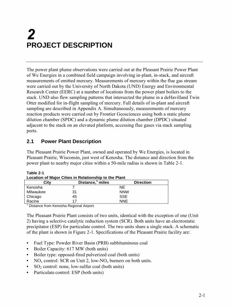
The power plant plume observations were carried out at the Pleasant Prairie Power Plantof We Energies in a combined field campaign involving in-plant, in-stack, and aircraftmeasurements of emitted mercury. Measurements of mercury within the flue gas streamwere carried out by the University of North Dakota (UND) Energy and EnvironmentalResearch Center (EERC) at a number of locations from the power plant boilers to thestack. UND also flew sampling patterns that intersected the plume in a deHavilland TwinOtter modified for in-flight sampling of mercury. Full details of in-plant and aircraftsampling are described in Appendix A. Simultaneously, measurements of mercuryreaction products were carried out by Frontier Geosciences using both a static plumedilution chamber (SPDC) and a dynamic plume dilution chamber (DPDC) situatedadjacent to the stack on an elevated platform, accessing flue gases via stack samplingports.

2.1 Power Plant Description

The Pleasant Prairie Power Plant, owned and operated by We Energies, is located inPleasant Prairie, Wisconsin, just west of Kenosha. The distance and direction from thepower plant to nearby major cities within a 50-mile radius is shown in Table 2-1.

Table 2-1Location of Major Cities in Relationship to the Plant

City Distance,1 miles DirectionKenosha 7 NEMilwaukee 31 NNWChicago 45 SSERacine 17 NNE1 Distance from Kenosha Regional Airport.

The Pleasant Prairie Plant consists of two units, identical with the exception of one (Unit2) having a selective catalytic reduction system (SCR). Both units have an electrostaticprecipitator (ESP) for particulate control. The two units share a single stack. A schematicof the plant is shown in Figure 2-1. Specifications of the Pleasant Prairie facility are:

Fuel Type: Powder River Basin (PRB) subbituminous coal Boiler Capacity: 617 MW (both units) Boiler type: opposed-fired pulverized coal (both units) NOx control: SCR on Unit 2, low-NOx burners on both units. SO2 control: none, low-sulfur coal (both units) Particulate control: ESP (both units)

Project description

2-2

Figure 2-1Schematic of the Pleasant Prairie Power Plant

The analysis of the coal fired at the Pleasant Prairie Power Plant is shown in Table 4-2.The coal is typical of a PRB in that the Hg concentration is relatively low, <0.05 ppm, andthe chlorine content is very low, 10 ppm.

Table 2-2Pleasant Prairie Coal Analysis (on an as-received basis)

Component ValueHg, ppm (dry) 0.041

Chlorine, ppm (dry) 10Proximate Analysis

Moisture, wt% 30.0Volatile Matter, wt% 33.0Fixed Carbon, wt% 31.5

Ash, wt% 5.5Ultimate Analysis

Hydrogen, wt% 6.6Carbon, wt% 46.9

Nitrogen, wt% 0.9Sulfur, wt% 0.4

Oxygen, wt% 39.7Heating Value, Btu/lb 8,190

Fd, dscf/106 Btu* 9,519* Emission factor.

2.2 Mercury Analyzers

2.2.1 Aircraft Hg Measurement System

The Hg analyzer used in the aircraft was a Tekran® Model 2537A mercury vapor analyzercoupled with a Tekran® Model 1130 mercury speciation unit and a Tekran® Model 1135

Project description

2-3

particulate module. Figure 2-1 shows a schematic of the Tekran® components. Severalmodifications were made to the Tekran® setup:

Addition of an optional impactor Adding an external pump to pull an isokinetic sample from the probe Adding a probe and heated sample transfer line to the sample path Adding a soda-lime trap Adding a zero-air valve trigger

Figure 2-1Schematic of the Tekran Mercury System

The analyzer portion of the system (Model 2537A) uses cold-vapor atomic fluorescencespectroscopy (CVAFS). The system uses a gold-impregnated trap for preconcentrating theHg and separating it from potential interferences that degrade sensitivity. The denuder(Model 1130) and particulate modules (1135) are integrated with the analyzer and areautomated, allowing simultaneous monitor of Hg0, RGM, and particulate-bound Hgspecies during aircraft operations. One sampling cycle would consist of one hour’s samplerecovery and analysis, during periods when the aircraft was in both the free atmosphereand the plume environment; time within the plume environment was summed via recordsfrom the rapid-response NOx analyzer. Further details are provided in Appendix A.

2.2.2 Stack Hg Analyzer

A Tekran Hg analyzer (Model 2537A modified to operate at the higher concentrations ofHg found in flue gas) was used at the stack to provide Hg speciation data continuouslyduring the experimental period (August 25–September 6, 2003). The system is calibratedusing Hg0 as the primary standard. The Hg0 is contained in a closed vial, which is held ina thermostatic bath. The temperature of the Hg is monitored, and the amount of Hg isdetermined using vapor pressure calculations. The unit calibration proved stable over a24-hour period.

Project description

2-4

Upstream of the Tekran, a wet-chemistry PS Analytical conversion/pretreatment systemwas used. The purpose of the pretreatment/conversion system was to remove acid gases(HCl) that can swamp the gold traps, to convert all the Hg to Hg0 so that it can bemeasured by the atomic fluorescence detector, and to allow the instrument to speciate Hg.The wet-chemistry conversion unit used SnCl2 to convert all of the Hg to Hg0 prior toanalysis; a KCl solution was used to strip out the Hg2+ (for speciation purposes), and asodium hydroxide solution removed the acid gases.

2.3 NOx Analyzer

Aboard the aircraft, the zero-air valve on the Tekran Model 1130 pump module wastriggered using an ambient air NOx analyzer. It was expected that a NOx differentialbetween ambient air and the plume environment would be detectable well downwind ofthe stack. The detection of this gradient along with a global positioning system (GPS) wasthen used to determine the location of the plume and thereby control the zero-air valve. Arapid-response NOx analyzer was necessary to allow recording of NOx concentrationchanges as the aircraft crossed the edges of elevated plume concentrations, and assumedthat NOx dispersed identically with total gaseous mercury (TGM). The assumption ofneutral buoyancy and equivalent Froude numbers for all plume constituents at and beyondequivalent stack height and distance was used to calculate in-plume portions of the Hgconcentration.

The analyzer that was used for this project was a rapid response, dual-range TECO Model42C ambient air NOx analyzer. This analyzer was able to measure 0–50 ppb NOx in thelow range and up to 500 ppb NOx in the high range, which based on the test at Bowenappeared to be adequate. By the removal of an external filter and replacement of ¼” lineswith 1/8” Teflon lines, the analyzer response time from the inlet of the sample probe wasdecreased to 2 seconds. A separate TECO Model 111 calibration unit was used to calibratethe analyzer. The system required a tank of NO calibration gas and a source of zero air.The TECO Model 111 uses mass flow controllers to mix the calibration and zero gases toproduce a desired calibration concentration.

2.4 Plume Dilution ChambersDuring aircraft operations, and at times between measurements aloft, a static and (later) adynamic plume dilution chamber were operated from scaffolding attached to the outside ofthe Pleasant Prairie stack structure. The static plume dilution chamber (SPDC) (Figure 2-2)is a 0.5-m3 partially evacuated stainless steel flask into which, successively, flue gas andambient air (total of 3 to 5 l) are introduced. The SPDC is equipped with switchable capsallowing either artificial rainfall, artificial sunlight, or both to be introduced. Successivesamples are withdrawn from the SPDC and analyzed using a Tekran instrument to gaugethe changes in speciation and concentration of mercury that occur over the sampling period.

The flue gas diluted with filtered ambient air is allowed to react for a fixed amount of time,typically 4 minutes, before sampling begins. The air pressure is maintained near ambient (1atm) in the SPDC. Dilution ratios [ambient air:flue gas bulk concentrations] were held atapproximately 140:1. The Tekran determines the initial mass-balance of gas-phase Hg0.Simultaneously with flue gas introduction into the SPDC, speciation of the flue gas at the

Project description

2-5

stack probe was determined using the Ontario-Hydro method and the FMSS method(Frontier Geosciences). Semi-automated Hg speciation measurements in the SPDC werecarried out using a Tekran 2537A total gaseous Hg instrument with a KCl-denuder andparticulate filter inlet. This method has been shown in lab and field tests to be precise,accurate, and free of artifacts (Landis et al., 2002). Elemental Hg was determinedcontinuously in the SPDC using the Tekran 2537A. During the time that the Tekran 2537Ameasured Hg0, both gaseous Hg+2 and particulate Hg were collected by the KCl-denuderand filter inlet. By collecting a number of Hg+2 and particulate Hg samples in series, thechanges in these species could be monitored over time. This required several KCl-denudersand particulate filters be prepared for each sample run. After the conclusion of thesampling, the KCl-denuders and particulate filters were directly analyzed in the Tekran2537 by thermal desorption.

Figure 2-2Static Plume Dilution Chamber

3-1

3EXPERIMENTAL APPROACH

3.1 Plume Sampling

3.1.1 Aircraft Sampling Arcs

Following background sampling at a location upwind of the stack, aircraft sampling was doneusing cross-plume arcs at three locations downwind of the stack. The first location wasapproximately 1500 ft from the stack (the closest the plane was permitted to approach thestack), at approximately effective stack height (initial thermal equilibrium of the plume). Thesecond and third locations were approximately 5 and 10 miles downwind of the stack,respectively. Figures 3-1 through 3-4 are diagrams of the sampling locations and patterns thatwere done for each flight event. A number of different patterns were flown at the closestsampling point in an effort to maximize the time in the plume. At the other two locations, aracetrack pattern was flown. Aircraft position and time were determined using a GPS system.

Figure 3-1Flight Track on August 27, 2003


3-2




3-3

Figure 3-4Flight Track on September 2, 2003

Determining the altitude and direction of the plume was done based on a combination of visualinspection (location closest to the stack) and the measurements of NOx concentrations. Exceptfor the closest location, the Tekran Hg analyzer was triggered by a NOx set point.

In addition to plume sampling, a vertical Hg profile was established at a location about 15–20 km downwind of the plume. The first sample was taken in the plume (approximately2500 ft), and the second point was taken below the plume at 500 ft. Because of the limitedflight time, it was decided to climb to the highest sample point before dropping to the 8500-ftsample point.

Details of each sampling flight, including local weather conditions during the flights, arepresented in Appendix A of this report.

3.1.3 Plume-Sampling Procedures

A total of five flight days was carried out during the experimental period of August 25-September 6, 2003. The following steps were carried out prior to flight and during in-flightsampling(full description is found in Appendix A):

The Hg analyzer was zeroed and then calibrated using primary injections of Hg0. The NOx analyzer was zeroed and spanned. The particulate module and denuder system were manually desorbed to remove any

residual Hg. Zero-Hg ambient air was sampled through the entire system for one cycle.


3-4

Background samples were taken in the plane at a point approximately 5 miles upwind ofthe stack.

The plume was then located by visual means at the point nearest to the stack (~1500 ft),and Hg samples were taken over a 25-minute period.

After the plume was located at the 5-mile arc, the NOx trigger point was set at anappropriate level for that distance downwind of the stack to trigger sampling when theplume was entered.

After the analysis of the first sample was completed, Hg sampling was done for another25 minutes at the 5-mile location.

The process was repeated at a point in the plume 10 miles downwind of the stack.

3.2 Stack Sampling

For comparison with plume mercury samples, in-stack sampling was carried out simultaneouslyduring the flights. Hg sampling at the stack was carried out using the Ontario Hydro (OH) Hgspeciation sampling method and a continuous mercury monitor (CMM) placed at the stack exit.One OH sample was taken per flight day.

During the sampling period, it was expected that the two units at the Pleasant Prairie Plantwould be operating at or near normal operating conditions. Plant operating conditions (i.e.,load, O2, NOx, SO2, CO2) were logged by plant personnel during the sampling period. Fromplant data, operating conditions were relatively constant for each day. Since stack NOx valueswere used to calculate dilution ratios for the plume samples, relatively constant operatingconditions were required to allow application of ground-calculated dilution ratios to aircraft-collected data.:

NOxBackgroundNOxPlume

NOxBackgroundNOxStackRatioDilution

[Eq. 1]

Since one of the two Pleasant Prairie units had a selective catalytic reduction (SCR) deviceoperational, the NOx concentrations in the stack were somewhat lower than desired for aircraftplume measurement. It should be noted that the ESPs at Pleasant Prairie Power Plant were veryefficient (>99.8%), which is illustrated by the low opacity (<10%). As a result, the plume wasdifficult to find visually from the air even at the closest location to the stack.

The Hg measurements by the aircraft and at the stack were compared to SPDC located at thestack by Frontier Geosciences, Inc.

4-1

4RESULTS AND DISCUSSION

4.1 Stack Results at Pleasant Prairie

The Hg concentrations in the stack are shown in Table 4-1 and Figure 4-1 for OH and CMMsampling, respectively. As the results show in Table 4-1, the Hg concentrations were relativelyconstant during the entire duration of the project. The Hg2+ averaged 34.3% (65.7% Hg0) of thetotal Hg measured. These results were well-matched by the CMM as shown in Figure 4-1.

Table 4-1Stack Ontario Hydro Mercury Speciation Results

Date Particulate-Bound Hg,

µg/Nm3

Hg2+,

µg/Nm3*Hg0,

µg/Nm3Hg (total),

µg/Nm3Hg0 as a %

of TotalHg

Hg2+ as a% of Total

Hg

08/27/03 0.00 3.30 6.70 10.00 67.0 33.008/29/03 0.00 3.43 6.06 9.49 63.9 36.108/30/03 0.00 3.02 6.63 9.65 68.7 31.308/31/03 0.00 4.01 5.10 9.11 56.0 44.009/02/03 0.00 2.51 5.66 8.17 69.3 30.709/04/03 0.00 3.07 6.83 9.90 69.0 31.0

Average 0.00 3.22 6.16 9.39 65.7 34.3Std. Dev. 0.00 0.50 0.68 0.67 5.1 5.1

* All concentrations (µg/Nm3) are based on 1 atmosphere pressure and 20°C


4-2

Figure 4-1Stack CMM Mercury Speciation Results

4.2 Plume Results at Pleasant Prairie

A summary of the results from the plume sampling at the Pleasant Prairie Plant are presented inTable 4-2, with the average presented in Table 4-3. The plume Hg concentrations have beenconverted to equivalent stack concentrations and are presented as such. The complete data set ispresented in Appendix A.I, and an explanation of the data reduction procedure is presented inAppendix A.II.


4-3

Table 4-2Plume Mercury Speciation Data

Sample Point Nearest the Stack, µg/Nm3 Sample Point Nominally 5 miles fromStack, µg/Nm3

Sample Point Nominally10 miles from Stack, µg/Nm3

Hg0

SampleNo.

8-27 8-30 8-31 9-2 9-4 9-4 Avg. 8-27 8-30 8-31 9-2 Avg. 8-27 8-30 9-2 Avg.

1 6.0 6.4 1.6 5.5 16.2*

2.8 9.2 5.6 7.6 1.2 4.1 1.6

2 42.0 7.5 6.3 9.2 5.0 16.2 28.3 10.2 13.9 10.0 5.3 13.2 8.63 10.6 4.7 5.7 4.0 16.5 33.5 12.0 15.7 24.4 7.8 12.8 7.64 9.8 4.7 8.0 13.1 2.3 157.7 36.1 7.9 11.7 10.9 15.7 28.3 5.95 11.9 9.0 15.6 15.4 18.0 11.8 16.3 25.9 10.3 7.9 13.0 16.96 37.8 6.5 7.4 3.9 17.5 75.5 14.8 14.5 9.1 27.7 27.3 3.77 12.9 14.5 18.2 15.0 43.9 56.1 12.5 49.8 16.4 17.2 21.0 14.08 14.0 7.9 10.1 7.2 10.6 12.8 8.3 13.6 25.0 80.6 19.9 11.6 6.19 15.5 5.8 10.2 9.8 19.2 17.8 15.7 21.6 5.3 14.8 22.7 17.410 12.5 24.2 8.9 7.6 9.9 28.7 28.5 17.0 89.3 16.0 19.2 16.3 19.5

Avg. Hg0 11.7 9.6 9.1 6.5 10.0 18.6 11.4 13.8 12.0 19.8 8.9 13.6 14.4 15.7 6.8 12.3Std. Dev 2.9 6.2 3.9 1.9 5.3 5.4 4.1 9.8 2.7 13.6 2.1 4.6 5.8 7.4 4.0 4.8

Hg (part.) 0.04 0.05 0.06 0.03 0.05 0.15 0.06 0.07 0.11 0.18 0.05 0.10 0.10 0.17 0.01 0.09Std. Dev. – – – – – – 0.04 0.06 0.08

RGM 1.8 2.5 2.6 1.3 2.0 1.7 2.0 1.2 2.3 2.4 0.9 1.7 1.4 2.4 1.0 1.6Std. Dev. – – – – – – 0.5 – – – – 0.8 – – – 0.7

Total Hg 13.5 12.2 11.8 7.8 12.1 20.4 13.5 15.1 14.4 22.3 9.8 15.4 15.9 18.3 7.8 14.0Std. Dev. – – – – – – 4.1 – – – – 5.2 – – – 5.5

% Hg0 86.4 78.8 77.4 83.0 83.0 91.0 84.7 91.6 83.3 88.5 90.4 88.3 90.6 85.9 87.1 87.9% Hg(part) 0.3 0.5 0.5 0.4 0.4 0.7 0.4 0.5 0.8 0.8 0.5 0.6 0.6 0.9 0.1 0.6% RGM 13.3 20.7 22.1 16.6 16.6 8.3 14.9 8.0 16.0 10.7 9.1 11.0 8.8 13.1 12.8 11.4

* The highlighted data were not used in calculating the averages or standard deviations.


4-4

Table 4-3Average Mercury Speciation Results for Each Location (from Table 6-2)*

Hgp, µg/Nm3 Hg0, µg/Nm3 RGM, µg/Nm3 Total Hg,µg/Nm3

% Hg0

In the StackAverage 0.00 3.2 6.2 9.4 65.7Std. Dev. 0.00 0.5 0.7 0.7 5.1

Location Nearest the Stack (~1500 ft)Average 0.06 11.4 2.0 13.5 84.7Std. Dev. 0.04 4.1 0.5 4.1 5.0

Location Nominally 5 miles from StackAverage 0.10 13.6 1.7 15.4 88.3Std. Dev. 0.06 4.6 0.8 5.2 4.0

Location Nominally 10 miles from StackAverage 0.09 12.3 1.6 14.0 87.9Std. Dev. 0.08 4.8 0.7 5.5 2.6


4.2.1 Data Censoring

After the data were reduced, examination revealed a number of high Hg0 concentrations thatcorresponded to very high dilution ratios (a high dilution ratio is defined as one greater than 3times the average when that point is removed). The high dilution ratios occurred duringintermittent aircraft transit of smaller plume eddies separated from the main body of the plume.These areas had relatively high proportions of ambient air sampled in short times and are notstatistically characteristic of the plume material at that distance from the stack. During thesesampling episodes, the NOx concentration would be just high enough to trigger the zero-airinlet valve to shut off and begin the sampling process. Once the valve was triggered, the valvewas set with a delay to stay off for 5 seconds once the NOx level again fell below the triggerpoint. This was done to prevent rapid cycling of the valve, which would make the data nearlyimpossible to resolve. The highlighted data shown in Table 4-2 are those data points that werecalculated based on high dilution ratios and were not used in the averages or determining themass balances.

4.2.2 Mass Balance Calculations

The stack Hg concentration data were normalized to 3% O2, 0C, and 1 atmosphere. The plumedata are also reported at 0C and 1 atmosphere for comparison on an equal basis. The plumedata were reduced by first correcting for the amount of sampling time in the plume. This allowsa Hg concentration in the plume to be calculated. The plume concentrations were thenconverted to an equivalent stack concentration by applying dilution factors which were basedon the plume and stack NOx concentrations (shown previously in Equation 1). A completeexplanation and examples of the data reduction procedures are presented in Appendix A.II. A


4-5

mass balance was calculated using the average total Hg data from each sampling point each dayand the corresponding stack data. The results are presented in Table 4-4. Although many of themass balance closures are somewhat high, they are quite reasonable considering the variabilityof the data and the difficult nature of the sampling. The most likely causes for the high Hgconcentration are underreported NOx concentration or Hg offgassing from the soda-lime trapsused in the aircraft Hg analyzer when exposed to plume gas. These will be discussed in detail inSection 6.2.3.


4-6

Table 4-4Total Hg Mass Balance: Plume Hg Compared to Stack Hg



TotalHg in

Plume,µg/Nm3


Balance,%

TotalHg in

Plume,µg/Nm3


Balance,%

TotalHg in

Plume,µg/Nm3


Balance,%

13.5 9.3 145 15.1 9.3 162 15.9 9.3 17112.2 8.5 144 14.4 8.5 169 18.3 8.5 21511.8 7.6 155 22.3 7.6 293 7.8 9.2 857.8 9.2 85 9.8 9.2 10512.1 9.2 13120.4 9.2 221

4.2.3 Plume Hg Speciation Results

Figure 4-2 is a plot of the average percentage of Hg0 in the plume as it moves from the stack to10 miles downwind of the stack. There is a substantial increase in the relative concentration ofHg0 from the stack to the first sample point, a smaller increase from the first to the secondsample point, and then no change to the last sample location (10 miles). Overall, the Hg0

increases from 67% of the total Hg to 88% by the time it reaches the 5-mile sample point. Thisis clearly seen in Figure 4-3. The question arises, is this increase real or does it represent a highbias in the Hg0 concentration measurements in the plume? Figure 4-4 plots the average totalplume Hg concentrations (as equivalent stack concentrations) at each location for each day ofsampling. The graph shows that the total Hg concentration increased (4 of the 5 days) from thestack to the location nearest the stack and then remains relatively constant as the plume movesdownwind. Figure 4-5 plots the RGM concentrations for each sampling point each day andshows that the RGM fraction decreases as the plume moves from the stack downwind. Overall,several factors could cause the Hg0 concentration (and total Hg) to be reported higher in theplume than in the stack including:

Low background Hg readings Inefficient trapping of the RGM in the Tekran denuder system Underreported plume NOx concentrations Integration errors of the NOx data Problems with the soda-lime traps

Each of these possibilities is discussed in more detail in Appendix A.


4-7

Figure 4-2Plot of the Concentration of Hg0 in the Plume As It Moves from the Stack to 10 miles Downwindof the Stack

Figure 4-3Plot of the % Hg0 in the Plume Compared to the Stack Hg Concentration As a Function ofDistance from the Stack


4-8

Figure 4-4Plot of the Concentration of Total Mercury in the Plume As It Moves from the Stack to 10 milesDownwind of the Stack

Figure 4-5Plot of the Concentration of RGM in the Plume As It Moves from the Stack to 10 miles Downwindof the Stack


4-9

4.3 Vertical Mercury Profile

In addition to plume sampling, a vertical sounding flight was carried out to measure Hgconcentration as a function of altitude. The first sample was collected 10 miles downwind ofthe power plant stack at an approximate altitude of 2500 feet, within the plume. The secondsample point was at an approximate altitude of 500 feet and may have been in the plume. TheNOx concentrations at the 500-foot elevation were higher than at the 2500-foot elevation. Thesehigher levels may have been caused by the plume, but may also be attributed to surface vehicleemissions from an underlying highway running north–south to the east of the sampling point.The third sampling point was at an approximate altitude of 16,500 feet, and the final samplepoint was at 8500 feet.

The results from this flight are presented in Table 4-5. The Hg concentrations at the two lowerelevations are presented as measured. Any Hg contributed by the plume has not beensubtracted, and no time correction has been made. The results show there is a significantincrease in particulate-bound Hg above the boundary layer and that the RGM remains elevatedabove the background concentrations measured in the boundary layer.

Table 4-5Vertical Profile Data

@ 500 ft @ 2500 ft @ 8500 ft @ 16,500 ft Background

Hg0 Sample No. Hg0 Concentration, ng/Nm3

1 1.142 1.292 1.151 0.687 0.9612 1.400 1.616 0.968 0.547 1.3693 1.650 1.824 0.814 0.437 1.5334 1.795 1.686 0.881 0.493 1.5035 1.516 1.748 0.828 0.428 1.6136 1.532 1.791 0.704 0.370 1.5147 1.567 1.590 0.873 0.312 1.7018 1.636 1.625 0.812 0.329 0.6599 1.903 1.322 0.753 0.288 0.313

10 1.409 1.678 0.751 0.322 0.890

Average 1.555 1.617 0.853 0.421 1.539

Non-Hg0 Concentrations, pg/Nm3

Hg(part.) 6.812 3.478 29.99 120.2 3.772RGM 70.968 63.12 55.80 86.05 7.178


4-10

4.4 Static Plume Dilution Chamber Findings

As a supplement to the direct mercury speciation measurements carried out within the plant, atthe stack, and aloft by aircraft, the Static Plume Dilution Chamber (SPDC) was run during ornearly in time with the aircraft soundings. The purpose of the SPDC runs during the experimentwas to determine whether an alternative, less expensive measurement method could beemployed for wider field measurement that would simulate plume chemistry at many powerplants. Method testing of the SPDC simulation chamber along with full-scale measurements ata number of operating power plants would, if the method is verified by its replicating full-scalemeasurements, allow faster and more efficacious determination of plume mercurytransformations at a great number of power plants. Such widespread use of an indirect, butreplicative, method would allow more rapid closure on potential chemical mechanisms for anyredox reactions, as well as allowing development of an iterative or projective computationalmethod for redox rates and products in plumes to be applied to national modeling exercises.

Table 4-6 displays results from the SPDC runs at Pleasant Prairie. As is evident, the SPDCmeasurements, using both the automated Tekran device and the Fluegas Mercury SorbentSpeciation (FMSS) method, using wet chemistry and sorbent traps, failed to replicate the aircraftmeasurements of Hg+2 reduction in part to Hg0. Indeed, the SPDC method in this case exhibited arelative loss of Hg0 over time within the dilution chamber. Only Run 2 on 29 August 2003appeared to show a reduction of the fraction occurring as Hg+2 and a relative increase of Hg0over the 2.5 minute observation time elapsed from dilution of the intake flue gas by ambient air.Thus, the SPDC was unable to replicate the measured full-scale reduction of divalent toelemental mercury in the Pleasant Prairie plant emissions plume.


4-11

Table 4-6Static Plume Dilution Chamber Results for Pleasant Prairie Power Plant Runs

Run ID 0828-S1 0829-S2 0830-S3 0831-S4 Mean Mean %Units

ng - 14.16 20.36 45.23 26.6 95%

ng 1.52 2.01 1.00 1.06 1.4 4.9%

Background Hg0 ng/m3 2.64 3.50 1.75 1.84 2.4

Expected Min. Hg0 ng/m3 2.67 22.18 30.79 53.39 35.5Observed Hg0 ng/m3 4.21 21.17 28.62 45.40 31.7

Observed % Hg0 % 158% 95% 93% 85% 89%ng 1.74 10.67 15.30 23.35 16.44 68%

ng - 9.89 4.12 9.68 7.9 32%

ng - 20.56 19.42 33.03 24.3ng - 16.18 21.37 46.29 27.9

- 127% 91% 71% 96% 28.3%

with FMSS only

Hg0 Expected ng/m3 2.67 22.18 30.79 53.39 42.09Hg0 Measured ng/m3 4.21 21.17 28.62 45.40 37.01Hg0 Net ng/m3 1.54 -1.01 -2.17 -7.99 -5.08 -12%

ng 0.77 -0.51 -1.09 -4.00 -2.54Hg(II) input ng - 4.8 5.8 19.5 12.65Hg(II) to Hg0 conversion % - -10% -19% -21% -0.20 5.3%

Measured/Expected %

SPDC Background**

Conditions, Files, Temp.

Calcultions at T = 2.5 minutes

Measured SPDC Rinse

Measured SPDC Gas Phase

Expected Total Hg in SPDC

Pleasant Prairie Power Plant (P4) SPDC Data Summary

Measured Total Hg in SPDC

Input to SPDC

*Fluegas Mercury Sorbent Speciation (FMSS) Method

5-1

5CONCLUSIONS AND RECOMMENDATIONS

Based on the overall testing program at the Pleasant Prairie Power Plant, the followingconclusions can be supported:

Using a dilution factor based on the plume and stack NOx, a reasonable Hg mass balancecan be obtained when the Hg in the stack is compared to the Hg in the plume.

There appeared to be a chemical reduction in divalent mercury in the Pleasant Prairie PowerPlant plume when the RGM in the plume is compared to the RGM in the stack. This reductionis matched by a corresponding increase in the proportion of Hg0. Overall, there was a 44%reduction of RGM from the stack to the first sample point near the effective stack height, and a66% reduction of RGM from the stack to the 5-mile sample point, with no additional reductionobserved between the 5- and 10-mile locations.

Although the results from the ground and aircraft measurements of this test tend to support areduction in RGM and a corresponding increase in Hg0 in the plume, those results are still notdefinitive. The SPDC tests failed to show a similar reduction, instead showing an apparent netoxidation in the simulated plume. In addition, although the earlier measurements in this series(at Georgia Power Plant Bowen in 2002) also showed plume mercury reductions, and werematched there by SPDC measurements, additional measurements in a wider range of sourceand ambient conditions are needed. Also, a reasonable chemical mechanism for such reductionreactions is still lacking. A primary need is for a mechanism to be developed that can explainthe results observed in non-heterogeneous (though generally not homogeneous) plumeconditions.

In planning future field tests of this type, experimental sites with the following generalcharacteristics should be sought:

Predicted fraction of emitted mercury occurring at stack exit as Hg+2 is greater than70%.

Has a single stack to prevent complications from merged plumes exhausting furnaces orfuel feeds with large differences.

Does not employee SCR technology (to favor higher concentrations of NOx as a co-tracer for the plume).

Is relatively isolated from other upwind and near-downwind sources of atmosphericmercury.

6REFERENCES

1. Toxicological Effects of Methylmercury. National Academies Press, Washington, D.C.,2000.

2. Lindqvist, O.; Rodhe, H. Atmospheric Mercury—A Review. Tellus 1995, 37B, 136–159.

3. Danilchik, P; Imhoff, R.; Liang, L.; Valente, R.; Dismukes, E.; Brown, C.; Spurling, D.;Huang, Z.; Prestbo, E. A Comparison of the Fate of Mercury in Flues and Plumes of Coal-Fired Boilers. Presented at the Mercury as a Global Pollutant Conference, July 10–14,1994, Whistler, British Columbia.

4. Imhoff, R.E. Preliminary Report on Measurements of Gas- and Particle-Phase Mercury inthe Plumes of Coal-Fired Boilers; Atmospheric Sciences Department, EnvironmentalResearch Center, Tennessee Valley Authority, March 15, 1995

5. Prestbo, E.M.; Calhoun, J.A.; Brunette, R.C.; Paladini, M. Hg Speciation in a SimulatedCoal Combustion Plume. In Proceedings of Air Quality: Mercury, Trace Elements, andParticulate Matter Conference; McLean, VA, Dec 1–4, 1998.

6. Laudal, D.L; Prestbo, E. Investigation of the Fate of Mercury in a Coal Combustion PlumeUsing a Static Plume Dilution Chamber; Final Report for U.S. Department of EnergyContract No. DE-FC-26-95FT40321; Energy & Environmental Research Center: GrandForks, ND, Oct 2001.

7. Edgerton, E.; Hartsell, B.; Jansen, J. Field Observations of Mercury Partitioning in PowerPlant Plumes. In Proceedings of the International Conference on Air Quality III: Mercury,Trace Elements, and Particulate Matter; Arlington, VA, Sept 2002

8. Banic, C.M.; Beauchamp, S.T.; Tordon, R.J.; Schroeder, W.H.; Steffen, A.; Anlauf, K.A.;Wong, H.K.T. Vertical Distribution of Gaseous Elemental Mercury in Canada. J. Geophys.Res. 2003, 108 (D9), 4264.

APPENDIX A

EPRI Project ManagerL. Levin

EPRI • 3412 Hillview Avenue, Palo Alto, California 94304 • PO Box 10412, Palo Alto, California 94303 • USA800.313.3774 • 650.855.2121 • [email protected] • www.epri.com

Evaluation of Mercury Speciation ina Power Plant PlumeProduct ID 1011113

Final Report, May 2005

Cosponsor(s)Energy & Environmental Research Center15 North 23rd StreetGrand Forks, ND, 58203

Project ManagerD. Laudal

APPENDIX A

DISCLAIMER OF WARRANTIES AND LIMITATION OF LIABILITIES

THIS DOCUMENT WAS PREPARED BY THE ORGANIZATION(S) NAMED BELOW AS ANACCOUNT OF WORK SPONSORED OR COSPONSORED BY THE ELECTRIC POWER RESEARCHINSTITUTE, INC. (EPRI). NEITHER EPRI, ANY MEMBER OF EPRI, ANY COSPONSOR, THEORGANIZATION(S) BELOW, NOR ANY PERSON ACTING ON BEHALF OF ANY OF THEM:

(A) MAKES ANY WARRANTY OR REPRESENTATION WHATSOEVER, EXPRESS OR IMPLIED, (I)WITH RESPECT TO THE USE OF ANY INFORMATION, APPARATUS, METHOD, PROCESS, ORSIMILAR ITEM DISCLOSED IN THIS DOCUMENT, INCLUDING MERCHANTABILITY AND FITNESSFOR A PARTICULAR PURPOSE, OR (II) THAT SUCH USE DOES NOT INFRINGE ON ORINTERFERE WITH PRIVATELY OWNED RIGHTS, INCLUDING ANY PARTY'S INTELLECTUALPROPERTY, OR (III) THAT THIS DOCUMENT IS SUITABLE TO ANY PARTICULAR USER'SCIRCUMSTANCE; OR

(B) ASSUMES RESPONSIBILITY FOR ANY DAMAGES OR OTHER LIABILITY WHATSOEVER(INCLUDING ANY CONSEQUENTIAL DAMAGES, EVEN IF EPRI OR ANY EPRI REPRESENTATIVEHAS BEEN ADVISED OF THE POSSIBILITY OF SUCH DAMAGES) RESULTING FROM YOURSELECTION OR USE OF THIS DOCUMENT OR ANY INFORMATION, APPARATUS, METHOD,PROCESS, OR SIMILAR ITEM DISCLOSED IN THIS DOCUMENT.

ORGANIZATION(S) THAT PREPARED THIS DOCUMENT

Energy & Environmental Research Center

ORDERING INFORMATION

Requests for copies of this report should be directed to EPRI Orders and Conferences, 1355 WillowWay, Suite 278, Concord, CA 94520. Toll-free number: 800.313.3774, press 2, or internally x5379;voice: 925.609.9169; fax: 925.609.1310.

Electric Power Research Institute and EPRI are registered service marks of the Electric PowerResearch Institute, Inc. EPRI. ELECTRIFY THE WORLD is a service mark of the Electric PowerResearch Institute, Inc.

Copyright © 2003 Electric Power Research Institute, Inc. All rights reserved.

APPENDIX A

iii

CITATIONS

This report was prepared by

Energy & Environmental Research Center15 North 23rd StreetGrand Forks, ND 58203

Principal InvestigatorD. Laudal

This report describes research sponsored by EPRI.

The report is a corporate document that should be cited in the literature in the following manner:

Evaluation of Mercury Speciation in a Power Plant Plume, EPRI, Palo Alto, CA, and Energy &Environmental Research Center, Grand Forks, ND: 2004. Product ID 1011113.

APPENDIX A

v

PRODUCT DESCRIPTION

Although in-stack mercury (Hg) speciation measurements are essential to the development ofcontrol technologies and to provide data for input into the atmospheric deposition models, thedetermination of speciation in a cooling coal combustion plume is more relevant for use inestimating Hg fate and effects through the atmosphere. Substantial research has been done in thepast on Hg transformations within energy conversion systems—determining the concentrationsof speciated Hg at the stack and doing ground-level atmospheric measurements; however, littlehas been done to determine the Hg chemistry, kinetics, and thermodynamics in the flue gasplume. It is the Hg transformations that occur in the plume that determine the rate and the formof Hg deposited in waterways. Therefore, a logical step in Hg research is to apply what we knowand extend this understanding beyond the power plant stack to the plume region. As a result, astudy was sponsored by EPRI and was jointly funded by EPRI, the U.S Department of Energy(DOE), and the Wisconsin Department of Administration. The study was designed to further ourunderstanding of plume chemistry.

Results & FindingsThere appeared to be a reduction in reactive gas mercury (RGM) (with a corresponding decreasein elemental mercury) at Pleasant Prairie when the RGM in the plume was compared to the RGMin the stack. There was a 44% reduction of RGM from the stack to the first sample point and a66% reduction of RGM from the stack to the 5-mile sample point, with no additional reductionbetween the 5- and 10-mile locations.

Challenges & ObjectivesSmaller-scale experiments in both test chambers and pilot-scale coal combustor exhaust streamshave indicated the presence of rapid and relatively complete reduction reactions convertingdivalent into elemental mercury within plumes representing partially dispersed conditions. Thepresence, rate, completeness, and ubiquity of these reactions, however, must be demonstrated inplume environments from fully operational power plant sources. That requirement, to captureeither the reactions or the reaction products of chemistry that may be occurring very close tostack exits in highly turbulent environments, constrains the precision and reproducibility of suchfull-scale experiments. The work described here is one of several initial steps required to testwhether, and in what direction, such rapid mercury redox reactions might be occurring in suchplumes.

Applications, Values & UseThe linking of mercury atmospheric sources and downwind receptors, particularly receivingwaters with the potential for fish enrichment of mercury, requires the use of atmospheric

APPENDIX A

vi

physicochemical models, since we lack benign chemical tracers that fully mimic the behavior ofmercury in the atmosphere. Current models either inadequately simulate chemical processes in-plume environments, or do not allow such inclusion at all. Establishing whether potentially rapidand complete mercury redox reactions occur in such environments, enriched in sulfur and otherco-emitted substances and not yet fully dispersed into the ambient atmosphere, will allow modelimprovements to better simulate contributions of those power plants where such reactions arelikely to occur. In turn, this will allow a better fit between model outcomes and actual processesin the atmosphere, to allow more realistic allocation of deposited mercury to its sources.

EPRI PerspectiveThe chemical form of inorganic Hg, whether elemental or divalent, strongly determines itssolubility in precipitable water in the atmosphere. This, in turn, may have orders of magnitudeeffects on ground-level concentrations and deposition rates near sources vs. long-rangedispersion. The work done at the Pleasant Prairie Power Plant is a fundamental contribution tounderstanding these differences mediated by the trace and major constituents in coal-fired powerplant stack plumes. The reactions implied may substantially alter the relative contributions ofnearby vs. distant sources to Hg deposition patterns.

ApproachThe overall project objective was to gain an understanding of Hg chemistry as a plume movesdownwind from the stack and to determine what changes occur. To accomplish this, a turbopropDHC-6-300 Twin Otter deHavilland Vistaliner aircraft and an automated Tekran ambient Hgmonitor were used. Aircraft sampling was done at three locations downwind of the plume. Thefirst location was approximately 1500 ft from the stack (the closest the plane could legally fly tothe stack). The second and third locations were approximately 5 and 10 miles downwind of thestack, respectively.


To establish baseline conditions for comparison with the plume samples, in-stack sampling wascompleted during the flight, providing measurements of the Hg speciation in the stack. Hgsampling at the stack was completed using the Ontario Hydro Hg speciation sampling methodand a continuous mercury monitor.

KeywordsMercuryUtilitiesPlume(s)Reactive Gaseous MercuryElemental MercuryAir Toxics

APPENDIX A

vii

ABSTRACT

Although in-stack mercury (Hg) speciation measurements are essential for the development ofHg control technologies and to provide source data for atmospheric deposition models, thedetermination of Hg speciation in a cooling coal combustion plume is more relevant for use inestimating Hg fate and effects through the atmosphere. It is the Hg transformations that occur inthe plume that determine the rate and the form of Hg deposited in waterways. Yet such processesare poorly understood and are not currently incorporated in atmospheric models of Hg.Therefore, a logical step in Hg research is to apply what we know and extend this understandingslightly beyond the power plant stack to the plume region. Therefore, EPRI and the U.S.Department of Energy have funded surface and aircraft studies of stack emissions and chemistryat two power plants. The first study was at Plant Bowen, Cartersville, Georgia, operated byGeorgia Power, part of Southern Company. Aircraft studies were conducted by Tennessee ValleyAuthority, with stack measurements by the Energy & Environmental Research Center (EERC)and by Frontier Geosciences. The second study was at the Pleasant Prairie Power Plant, PleasantPrairie, Wisconsin, operated by WE Energies; there, surface and aircraft measurements werecarried out by the EERC, with additional studies of the stack by Frontier Geosciences. Theprimary focus of this report is on the work conducted by the EERC at Pleasant Prairie.

The overall project objective was to gain an understanding of Hg chemistry as a plume istransported downwind from the stack. This was carried out by flying a Twin Otter aircraftthrough the plume at several locations (a point nearest the stack, 5 miles from the stack, and10 miles from the stack) and measure the speciated Hg composition in the plume using anautomated ambient Hg monitor.

The results of the project appeared to show a reduction in reactive gas mercury (RGM) (with acorresponding decrease in elemental Hg) when the RGM in the plume is compared to the RGMin the stack. There was a 44% reduction of RGM from the stack to the first sample point and a66% reduction of RGM from the stack to the 5-mile sample point, with no additional reductionbetween the 5- and 10-mile locations.

APPENDIX A

ix

ACKNOWLEDGMENTS

This work would not have been possible without the efforts of many people. The authors wouldlike to acknowledge the following people.

For their direction and leadership, recognition is given to Leonard Levin and Paul Chu of EPRIand William Aljoe and Lynn Brickett of the U.S. Department of Energy National EnergyTechnology Laboratory. The work could also not have been completed without funding supportfrom the Wisconsin Department of Administration.

At the University of North Dakota from the Energy & Environmental Research Center, thanks goto Grant Dunham, Blaise Mibek, and Richard Schulz and from the School of AerospaceSciences, David Delene.

We would also like to thank the other EPRI contractors who contributed to the effort, includingEric Prestbo from Frontier Geosciences and Ray Valente from the Tennessee Valley Authority.

Last, special thanks are expressed to WE Energies for allowing the testing to be conducted at thePleasant Prairie Power Plant and for all of the help their personnel gave us.

APPENDIX A

xi

NOMENCLATURE

AF atomic fluorescenceCEM continuous emission monitorCMM continuous mercury monitorCVAFS cold-vapor atomic fluorescence spectroscopyDOE U.S. Department of EnergyEERC Energy & Environmental Research CenterESP electrostatic precipitatorFd value relating gas volume to the heat content of the fuel, equal to dscf/106 BtuGEM gaseous elemental mercuryGPS global positioning systemHCl hydrochloric acidHg mercuryHg0 elemental mercuryHg2+ oxidized mercuryHYSPLIT HYbrid Single-Particle Lagrangian Integrated Trajectory modellpm liter per minuteMW megawattsnm nautical mileNOx nitrogen oxidesNOy reactive nitrogen speciesOH Ontario Hydro mercury speciation methodppb parts per billionPRB Powder River BasinRGM reactive gas mercurySCR selective catalytic reductionSnCl2 stannous chlorideSO2 sulfur dioxidesSPDC simultaneous plume dilution chamberTECO Thermal Electron CorporationTVA Tennessee Valley Authority

APPENDIX A

xiii

EXECUTIVE SUMMARY

The objective of this report is to provide a detailed summary of the results that the Energy &Environmental Research Center (EERC) obtained for the project entitled “Evaluation of MercurySpeciation in a Power Plant Plume.” The data were obtained during testing at the Pleasant PrairiePower Plant during August of 2003. The project was sponsored by EPRI with funding from theU.S. Department of Energy (DOE) National Energy Technology Laboratory and the WisconsinDepartment of Administration.

Introduction

Characterization of environmental mercury (Hg) and its atmospheric process, from emission todeposition, requires both measurement and model simulations for a full understanding. Althoughin-stack Hg speciation measurements are essential to the development of control technologiesand to provide data for input into the atmospheric deposition models, the determination ofspeciation in a cooling coal combustion plume is more relevant for use in estimating Hg fate andeffects through the atmosphere. Substantial research has been done in the past on Hgtransformations within energy conversion systems—determining the concentrations of speciatedHg at the stack and doing ground-level atmospheric measurements; however, little has been doneto determine the Hg chemistry, kinetics, and thermodynamics in the flue gas plume [1]. It is theHg transformations that occur in the plume that determine the rate and the form of Hg depositedin waterways. Therefore, a logical step in Hg research is to apply what we know and extend thisunderstanding beyond the power plant stack to the plume region.

Therefore, EPRI and DOE funded plume studies at two power plants. The first was at the BowenPower Plant (operated by Georgia Power, part of Southern Company), with the Tennessee ValleyAuthority (TVA) conducting the aircraft studies and the EERC and Frontier Geosciences doingHg measurements at the stack. The second study was conducted at the Pleasant Prairie PowerPlant, owned by WE Energies, with the EERC carrying out both the aircraft and stack Hgmeasurements, with additional surface measurements again done by Frontier Geosciences. Theprimary focus of this paper is the work conducted by the EERC at Pleasant Prairie. However, theimportance of the previous work conducted by TVA [2,3], the static plume dilution chamberwork done by Frontier Geosciences [1,4], and the measurements made by Atmosphere Research& Analysis [5] at the Yorkville SEARCH site indicating that there is change in Hg speciation inthe plume cannot be overstated.

Project Objectives

The overall project goal is to gain an understanding of Hg chemistry as a plume movesdownwind from the stack. Specific objective are as follows:

APPENDIX A

xiv

Develop sampling techniques to measure speciated Hg in the plume.

Develop techniques to determine the location of the plume at various points downwind of thestack.

Determine the speciated Hg emissions at the stack and compare these results to thoseobtained from the plume sampling.

Compute a Hg mass balance using dilution factors and other relevant parameters.

Project Description

Power Plant Description

The Pleasant Prairie Power Plant, owned and operated by WE Energies, is located near the cityof Pleasant Prairie just west of Kenosha, Wisconsin. The Pleasant Prairie plant consists of twounits (Units 1 and 2) identical in operation with the exception of one (Unit 2) having a selectivecatalytic reduction (SCR) system at the time of the measurements. Each unit has an electrostaticprecipitator (ESP) for particulate control and share a common stack. Specifications of thePleasant Prairie facility are as follows:

Fuel type: Powder River Basin (PRB) subbituminous coal

Boiler capacity: 617 MW (each unit)

Boiler type: opposed-fired pulverized coal (both units)

NOx control: SCR on Unit 2, low-NOx burners on both units

SO2 control: none, combustion of low-sulfur coal (both units)

Particulate control: ESP (both units)

The coal is fairly typical of PRB in that both the Hg and chlorine levels in the coal arecomparatively low; the Hg averaged 0.041 µg/g and the chlorine, 10 ppm.

Aircraft and Equipment Used for the Project

The aircraft used for the emission plume sampling was a turboprop DHC-6-300 Twin OtterdeHavilland Vistaliner, which is a highly maneuverable, versatile aircraft. The aircraft and crewwere provided by Twin Otter International out of Las Vegas, Nevada. The pilots were veryexperienced in doing research involving ambient air sampling. The aircraft is shown inFigure ES-1. This type of aircraft had a number of design and performance characteristics thatmade it an ideal platform for the project. The twin-engine plane had a relatively large capacityfor equipment and sufficient onboard electrical supply and could be operated efficiently at lowaltitudes. These capabilities were accompanied by relatively low fuel consumption at allaltitudes. Most importantly for the plume study project, it could be flown at relatively slowspeeds (80–160 knots/150–300 km/hr) and in tight formation to allow consistent plume traversesat fixed heights and downwind distances.

APPENDIX A

xv

Figure ES-1Photograph of the DHC-6-300 Twin Otter deHavilland Vistaliner

The Hg analyzer used in the aircraft (shown in Figure ES-2) was a fully automated Tekran®

Model 2537A mercury vapor analyzer coupled with a Tekran® Model 1130 mercury speciationunit and a Tekran® Model 1135 particulate module. The analyzer portion of the system is basedon the principle of atomic fluorescence and has detection limits <1 pg/m3. With this system, itwas possible to simultaneously measure elemental mercury (Hg0), reactive gas mercury (RGM),and particulate-bound Hg species during the flight. Therefore, it was possible to rapidly evaluatedata each day to make sampling decisions for succeeding flights.

Figure ES-2Schematic of the Tekran Mercury System

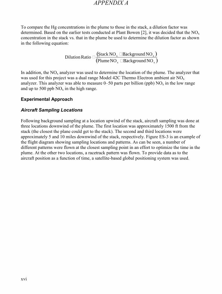
APPENDIX A

xvi

To compare the Hg concentrations in the plume to those in the stack, a dilution factor wasdetermined. Based on the earlier tests conducted at Plant Bowen [2], it was decided that the NOxconcentration in the stack vs. that in the plume be used to determine the dilution factor as shownin the following equation:

xx

xx

NOBackgroundNOPlume

NOBackgroundNOStackRatioDilution

In addition, the NOx analyzer was used to determine the location of the plume. The analyzer thatwas used for this project was a dual range Model 42C Thermo Electron ambient air NOxanalyzer. This analyzer was able to measure 0–50 parts per billion (ppb) NOx in the low rangeand up to 500 ppb NOx in the high range.


Aircraft Sampling Locations

Following background sampling at a location upwind of the stack, aircraft sampling was done atthree locations downwind of the plume. The first location was approximately 1500 ft from thestack (the closest the plane could get to the stack). The second and third locations wereapproximately 5 and 10 miles downwind of the stack, respectively. Figure ES-3 is an example ofthe flight diagram showing sampling locations and patterns. As can be seen, a number ofdifferent patterns were flown at the closest sampling point in an effort to optimize the time in theplume. At the other two locations, a racetrack pattern was flown. To provide data as to theaircraft position as a function of time, a satellite-based global positioning system was used.

APPENDIX A

xvii

Figure ES-3Flight Track on August 27, 2003


Aircraft sampling flights were conducted in daylight under atmospheric conditions that permittedadequate sampling of the stack plume. The weather conditions during the project were fairlyconsistent with the historical climate record with many fair weather days. In the original testplans, the ideal wind velocities were considered to be approximately 2.5–5 m/s; however, theaverage wind speeds were somewhat above this, ranging from 5.3 to 8.3 m/s. These windvelocities were still low enough that the aircraft was able to find the plume and good samplingwas able to be completed.

Stack Sampling

To establish baseline conditions for comparison with the plume samples, in-stack sampling wascarried out simultaneously with the flight, providing measurements of the Hg speciation in thestack. Hg sampling at the stack was completed using the Ontario Hydro (OH) Hg speciationsampling method and a continuous mercury monitor (CMM). Prior to the start of the testing, aCMM was placed at the stack outlet and remained there during the entire project. During eachflight day, one OH sample was taken at the stack.

In addition to Hg measurements by the EERC, the plant operators continuously measured theNOx concentration in the stack using a continuous emission monitor. Although the NOxconcentrations in the stack at the Pleasant Prairie Power Plant were somewhat lower than desired

APPENDIX A

xviii

for aircraft plume measurements (since half the flue gas was being treated using an SCR), it wasstill possible to detect a difference between the background and plume, even at 10 miles. Theaverage stack NOx concentration was 144 ppm(v).


Stack Results at Pleasant Prairie

The Hg concentrations in the stack are shown in Table ES-1 and the OH and CMM sampling inFigure ES-4. As the results show in Table ES-1, the Hg concentrations were relatively constantduring the entire duration of the project. The RGM averaged 34.3% of the total Hg measured.These results were matched very well by the CMM as shown in Figure ES-5.

Table ES-1Stack Ontario Hydro Mercury Speciation Results


µg/Nm3*

RGM, µg/Nm3 Hg0, µg/Nm3 Hg (total),µg/Nm3

RGM as a %of Total Hg

08/27/03 0.00 3.30 6.70 10.00 33.0

08/29/03 0.00 3.43 6.06 9.49 36.1

08/30/03 0.00 3.02 6.63 9.65 31.3

08/31/03 0.00 4.01 5.10 9.11 44.0

09/02/03 0.00 2.51 5.66 8.17 30.7

09/04/03 0.00 3.07 6.83 9.90 31.0

* All concentrations (µg/Nm3) are based on 1 atmosphere pressure and 20°C.

APPENDIX A

xix

Figure ES-4Stack CMM Speciation Results

Figure ES-5Plot of the % Hg0 in the Plume Compared to the Stack Hg Concentration as a Function ofDistance from the Stack

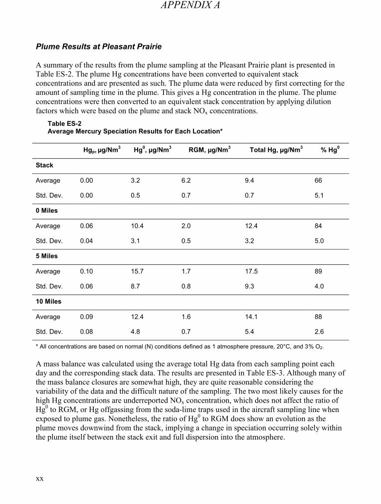
APPENDIX A

xx

Plume Results at Pleasant Prairie

A summary of the results from the plume sampling at the Pleasant Prairie plant is presented inTable ES-2. The plume Hg concentrations have been converted to equivalent stackconcentrations and are presented as such. The plume data were reduced by first correcting for theamount of sampling time in the plume. This gives a Hg concentration in the plume. The plumeconcentrations were then converted to an equivalent stack concentration by applying dilutionfactors which were based on the plume and stack NOx concentrations.

Table ES-2Average Mercury Speciation Results for Each Location*

Hgp, µg/Nm3 Hg0, µg/Nm3 RGM, µg/Nm3 Total Hg, µg/Nm3 % Hg0

Stack

Average 0.00 3.2 6.2 9.4 66

Std. Dev. 0.00 0.5 0.7 0.7 5.1

0 Miles

Average 0.06 10.4 2.0 12.4 84

Std. Dev. 0.04 3.1 0.5 3.2 5.0

5 Miles

Average 0.10 15.7 1.7 17.5 89

Std. Dev. 0.06 8.7 0.8 9.3 4.0

10 Miles

Average 0.09 12.4 1.6 14.1 88

Std. Dev. 0.08 4.8 0.7 5.4 2.6


A mass balance was calculated using the average total Hg data from each sampling point eachday and the corresponding stack data. The results are presented in Table ES-3. Although many ofthe mass balance closures are somewhat high, they are quite reasonable considering thevariability of the data and the difficult nature of the sampling. The two most likely causes for thehigh Hg concentrations are underreported NOx concentration, which does not affect the ratio ofHg0 to RGM, or Hg offgassing from the soda-lime traps used in the aircraft sampling line whenexposed to plume gas. Nonetheless, the ratio of Hg0 to RGM does show an evolution as theplume moves downwind from the stack, implying a change in speciation occurring solely withinthe plume itself between the stack exit and full dispersion into the atmosphere.

APPENDIX A

xxi

Table ES-3Total Hg Mass Balance: Plume Hg Compared to Stack Hg



Total Hgin

Plume,µg/Nm3

Total Hgin

Stack,µg/Nm3

Balance,%

Total Hgin

Plume,µg/Nm3

Total Hgin

Stack,µg/Nm3

Balance,%

Total Hgin

Plume,µg/Nm3

Total Hgin

Stack,µg/Nm3

Balance,%

13.5 9.3 145 15.1 9.3 162 16.5 9.3 177

12.2 8.5 144 14.4 8.5 169 17.8 8.5 209

10.8 7.6 142 22.2 7.6 292 7.9 9.2 86

7.8 9.2 85 9.6 9.2 104

12.0 9.2 130

18.6 9.2 202

It should be noted there were a number of high readings that corresponded to very high dilutionratios. These results were not included in the average. The high dilution ratios occurred duringintermittent aircraft transit of smaller plume eddies separated from the main body of the plume.When this occurs, relatively high proportions of ambient air is sampled in a short time and is,therefore, not statistically characteristic of the plume material at that distance from the stack.Even with relatively stable winds, turbulent eddies would result in complex plume structures,causing some passes through the plume to only intersect edges of the plume rather than the cross-centerline transects that were sought. These peripheral intersects would capture relatively largeproportions of ambient air with markedly lower NOx values than the main body of the plume.During these sampling episodes, the NOx concentration would be just high enough to trigger thezero air inlet valve in the sampling system. Once it was triggered, the valve was set with a delayto stay off for 5 seconds once the NOx level again fell below the trigger point. This was done toprevent rapid cycling of the valve. Since the NOx concentration was near ambient levels in thesesegments of the plume, the resulting dilution ratios were artificially high.

The overall results are shown in Figure ES-4 in a plot of the average percentage of Hg0 in theplume as it moves from the stack exit to 10 miles downwind of the stack. There is a substantialincrease in the concentration of Hg0 from the stack to the first sample point, a smaller increasefrom the first to the second sample point, and then no change from there to the last samplelocation (10 miles). Overall, the Hg0 increases from 67% of the total Hg to 89% by the time itreaches the 5-mile sample point.

The question arises, is this increase real, or does it represent a high bias in the Hg0 concentrationmeasurement in the plume? Several factors could cause the Hg0 concentration (and total Hg) tobe reported higher in the plume than in the stack. These include the following:

Low background Hg readings

APPENDIX A

xxii

Inefficient trapping of the RGM in the Tekran denuder

Underreported plume NOx concentrations

Problems with the soda-lime traps

Low Background Mercury Readings

The subtraction of low background concentrations from the measured plume concentrationswould result in higher in-plume Hg concentrations when they are converted to equivalent stackHg concentrations. However, this does not appear to be the case because the measuredbackground concentrations were fairly consistent and in the expected range. Also, lowbackground RGM concentrations would have caused those values to be higher as well, and this isnot the case.

Inefficient Trapping of the RGM in the Annular Denuder

If the RGM were not trapped in the denuder but passed through to the analyzer, it would bereported as Hg0. However, if the RGM were to pass through the annular denuder, it would mostlikely be trapped on the particulate filter and be reported instead as particulate-bound Hg. Thedata for the particulate-bound Hg concentrations do not suggest this was the case.

Underreported Plume NOx Concentrations

This would result in larger dilution ratios and higher equivalent stack concentrations, but itwould affect both the Hg0 and the RGM concentrations. However, if the plume NOxconcentrations were underreported, it would affect both the Hg0 and RGM concentrations in thesame sense, and this is clearly not the case.

Problems with the Soda-Lime Traps

Modified soda-lime traps were used to scrub acid gases from the sample gas stream before itreached the Hg analyzer. At the Bowen Plant, it was observed that Hg desorbed from these trapswhen they were exposed to ambient air rather than the scrubbed zero air. There did not appear tobe any offgassing of Hg when ambient air was sampled at the Pleasant Prairie Plant, but adifferent type of soda lime trap (supplied by Frontier GeoSciences) was used.

Conclusions

The following conclusions can be stated based on the Pleasant Prairie Power Plant stack andplume Hg sampling:

Hg can be measured by aircraft in plumes with reasonable accuracy and precision. However,great care must be taken to prevent contamination in sampling lines and equipment usedaboard the aircraft.

Using a dilution factor based on the plume and stack NOx, a reasonable Hg mass balance canbe obtained to compare the Hg in the stack to the Hg in the plume.

APPENDIX A

xxiii

There appeared to be a decline in the fraction of RGM at Pleasant Prairie when values in theplume are compared to those in the stack (with a corresponding increase in the proportion ofHg0). There was a 38% reduction of RGM between the in-stack measurement and the firstsample point closest to the stack, and a 47% reduction of RGM from the stack to the 5-milesample point, with no additional reduction between the 5- and 10-mile locations. This isconsistent with earlier measurements by Frontier Geosciences of Hg reduction reactions in itsstatic plume dilution chamber, which indicated rapid reduction reactions after flue gasemissions were mixed with ambient air in conditions representing the region just outside ofthe stack exit.

References

1. Prestbo, E.M.; Calhoun, J.A.; Brunette, R.C.; Paladini, M. Hg Speciation in a Simulated CoalCombustion Plume. In Proceedings of Air Quality: Mercury, Trace Elements, andParticulate Matter Conference; McLean, VA, Dec 1–4, 1998.

2. Danilchik, P; Imhoff, R.; Liang, L.; Valente, R.; Dismukes, E.; Brown, C.; Spurling, D.;Huang, Z.; Prestbo, E. A Comparison of the Fate of Mercury in Flues and Plumes of Coal-Fired Boilers. Presented at the Mercury as a Global Pollutant Conference, July 10–14, 1994,Whistler, British Columbia.

3. Imhoff, R.E. Preliminary Report on Measurements of Gas- and Particle-Phase Mercury inthe Plumes of Coal-Fired Boilers; Atmospheric Sciences Department, EnvironmentalResearch Center, Tennessee Valley Authority, March 15, 1995.


5. Edgerton, E.; Hartsell, B.; Jansen, J. Field Observations of Mercury Partitioning in PowerPlant Plumes. In Proceedings of the International Conference on Air Quality III: Mercury,Trace Elements, and Particulate Matter; Arlington, VA, Sept 2002.

APPENDIX A

xxv

CONTENTS

1 INTRODUCTION ..................................................................................................................1-1

2 BACKGROUND ...................................................................................................................2-12.1 Field Observations of Mercury Partitioning in Power Plant Plumes ............................2-1

2.2 Airborne Measurement of Plume Mercury at Plant Bowen, Cartersville, Georgia .......2-2

3 PROJECT OBJECTIVES .....................................................................................................3-1

4 PROJECT DESCRIPTION....................................................................................................4-14.1 Power Plant Description.............................................................................................4-1

4.2 Aircraft .......................................................................................................................4-3

4.3 Mercury Analyzers .....................................................................................................4-5

4.3.1 Aircraft Hg Measurement System......................................................................4-5

Instrument Sampling Sequence .................................................................................4-6

4.3.2 Stack Hg Analyzer.............................................................................................4-8

4.4 NOx Analyzer .............................................................................................................4-9

4.5 Other Equipment........................................................................................................4-9

5 EXPERIMENTAL APPROACH ............................................................................................5-15.1 Plume Sampling.........................................................................................................5-1

5.1.1 Aircraft Sampling Locations...............................................................................5-1

5.1.2 Plume-Sampling Weather Conditions ................................................................5-3

5.1.3 Plume-Sampling Procedures Used..................................................................5-10

Preflight ...................................................................................................................5-10

In-Flight....................................................................................................................5-10

5.2 Stack Sampling........................................................................................................5-11

6 RESULTS AND DISCUSSION .............................................................................................6-16.1 Stack Results at Pleasant Prairie ...............................................................................6-1

APPENDIX A

xxvi

6.2 Plume Results at Pleasant Prairie..............................................................................6-2

6.2.1 Data Outliers .....................................................................................................6-4

6.2.2 Mass Balance Calculations ...............................................................................6-5

6.2.3 Plume Hg Speciation Results ............................................................................6-6

Low Background Mercury Readings ..........................................................................6-9

Inefficient Trapping of the RGM in the Annular Denuder ............................................6-9

Underreported Plume NOx Concentrations.................................................................6-9

Integration Errors of the NOx Data ...........................................................................6-10

Problems with the Soda-Lime Traps ........................................................................6-10

6.3 Vertical Mercury Profile ............................................................................................6-10

7 CONCLUSIONS AND RECOMMENDATIONS.....................................................................7-1

8 REFERENCES .....................................................................................................................8-1

A MERCURY WORKSHEETS................................................................................................ A-1

B DATA REDUCTION PROCEDURES .................................................................................. A-1

APPENDIX A

xxvii

LIST OF FIGURES

Figure 2-1 Schematic of the Hg-Sampling System Used by TVA at the Bowen PowerPlant.................................................................................................................................2-3

Figure 2-2 Changes in RGM Normalized by NOx As a Function of Distance from theStack................................................................................................................................2-5

Figure 4-1 Schematic of the Pleasant Prairie Power Plant .......................................................4-2Figure 4-2 Aerial Photograph of the Pleasant Prairie Power Plant ...........................................4-2Figure 4-3 Photograph of the DHC-6-300 Twin Otter deHavilland Vistaliner ............................4-4Figure 4-4 Photograph Showing External Sampling Probe on Aircraft .....................................4-5Figure 4-5 Schematic of the Tekran Mercury System ..............................................................4-6Figure 4-6 Illustration of the Sampling and Desorption Phases of the Tekran Model 1130.......4-7Figure 5-1 Flight Track on August 27, 2003 .............................................................................5-1Figure 5-2 Flight Track on August 30, 2003 .............................................................................5-2Figure 5-3 Flight Track on August 31, 2003 .............................................................................5-2Figure 5-4 Flight Track on September 2, 2003.........................................................................5-3Figure 5-5 Weather Conditions During the August 27, 2003, Plume-Sampling Flight...............5-5Figure 5-6 Weather Conditions During the August 30, 2003, Plume-Sampling Flight...............5-6Figure 5-7 Weather Conditions During the August 31, 2003, Plume-Sampling Flight...............5-7Figure 5-8 Weather Conditions During the September 2, 2003, Plume-Sampling Flight...........5-8Figure 5-9 Weather Conditions During the September 4, 2003, Plume-Sampling Flight...........5-9Figure 5-10 View of the Plume from the Air and from the Ground ..........................................5-12Figure 6-1 Stack CMM Mercury Speciation Results .................................................................6-2Figure 6-2 Plot of the Concentration of Hg0 in the Plume As It Moves from the Stack to

10 miles Downwind of the Stack.......................................................................................6-7Figure 6-3 Plot of the % Hg0 in the Plume Compared to the Stack Hg Concentration As a

Function of Distance from the Stack.................................................................................6-7Figure 6-4 Plot of the Concentration of Total Mercury in the Plume As It Moves from the

Stack to 10 miles Downwind of the Stack.........................................................................6-8Figure 6-5 Plot of the Concentration of RGM in the Plume As It Moves from the Stack to

10 miles Downwind of the Stack.......................................................................................6-8

APPENDIX A

xxix

LIST OF TABLES

Table 4-1 Location of Major Cities in Relationship to the Plant................................................4-1Table 4-2 Pleasant Prairie Coal Analysis ................................................................................4-3Table 5-1 Wind Velocities for Each Day of Plume Sampling with the Aircraft (10 a.m.

and 6 p.m. at the aircraft sampling level over Kenosha, Wisconsin) .................................5-4Table 5-2 Process Data as Measured at the Stack ...............................................................5-11Table 6-1 Stack Ontario Hydro Mercury Speciation Results....................................................6-1Table 6-2 Plume Mercury Speciation Data..............................................................................6-3Table 6-3 Average Mercury Speciation Results for Each Location..........................................6-4Table 6-4 Total Hg Mass Balance: Plume Hg Compared to Stack Hg.....................................6-6Table 6-5 Background Mercury Concentrations ......................................................................6-9Table 6-6 Vertical Profile Data ..............................................................................................6-11

Table A-1 Complete Data Mercury Worksheet: August 27, 2003 ............................................ A-2Table A-2 Complete Data Mercury Worksheet: August 30, 2003 ............................................ A-3Table A-3 Complete Data Mercury Worksheet: August 31, 2003 ............................................ A-4Table A-4 Complete Data Mercury Worksheet: September 2, 2003........................................ A-5Table A-5 Complete Data Mercury Worksheet: September 4, 2003........................................ A-6Table B-1 Data Format for Converting Plume Hg Data to Equivalent Stack Hg Data .............. A-2Table B-2 Format for Sample Time......................................................................................... A-3Table B-3 Sample Data Format .............................................................................................. A-4Table B-4 Sample Integration ................................................................................................. A-7

APPENDIX A

1-1

1INTRODUCTION

Mercury (Hg) is emitted by both natural and human processes and cycles through atmospheric,aquatic, and terrestrial environments. Forms of Hg that appear most important in theseenvironments are elemental mercury (Hg0), inorganic or oxidized Hg (primarily Hg2+), andmethylmercury. The chemical form of Hg affects its transport through air, land, and water, aswell as chemical and biological behavior. Hg0 is known to circulate in the atmosphere for about1 to 2 years before it is deposited [1]. Hg2+, also referred to as reactive gas mercury (RGM) byatmospheric scientists, in the atmosphere can be deposited directly to water bodies or can betransported from land by runoff and enter ponds, streams, rivers, lakes, etc. The water bodiescontain microorganisms that have the metabolic capability to carry out chemical reactions thatbind Hg2+ to methyl groups, producing methylmercury.

Although in-stack Hg speciation measurements are essential to the development of controltechnologies and to provide data for input into the atmospheric deposition models, thedetermination of speciation in a cooling coal combustion plume is more relevant for use inestimating Hg fate and effects through the atmosphere. Substantial research has been done in thepast on Hg transformations within energy conversion systems—determining the concentrationsof speciated Hg at the stack and doing ground-level atmospheric measurements; however, littlehas been done to determine the Hg chemistry, kinetics, and thermodynamics in the flue gasplume [2]. It is the Hg transformations that occur in the plume that determine the rate and theform of Hg deposited in waterways. Therefore, a logical step in Hg research is to apply what weknow and extend this understanding beyond the power plant stack to the plume region.Therefore, EPRI and the U.S. Department of Energy have funded stack and aircraft Hgmeasurements at two power plants. The primary focus of this report is work conducted by theEnergy & Environmental Research Center (EERC) at Pleasant Prairie.

APPENDIX A

2-1

2BACKGROUND

In the mid 90s the Tennessee Valley Authority (TVA) attempted to evaluate Hg in plumes withmixed success [3,4]. Also Frontier Geosciences developed a static dilution chamber to simulateHg chemistry downwind of a stack. Because of the rapid changes in Hg chemistry that occur andthe wall effects of a relatively small vessel, it was difficult to interpret the results [5,6]. Thesestudies clearly suggest that there are changes in the chemical form (Hg0 vs. Hg2+) and in thephysical state (gaseous vs. particulate) of Hg occurring as the plume moves downwind of thestack.

2.1 Field Observations of Mercury Partitioning in Power Plant Plumes

Measurements of Hg0, RGM, and total particulate Hg; SO2; reactive nitrogen species (NOy); CO;surface meteorology; and fine particle mass and composition were made at the Yorkville,Georgia, SEARCH site from 2001 through 2003 by Edgerton et al. [7]. Yorkville is a rural sitelocated approximately 55 km west-northwest of Atlanta, Georgia, and 40 km south-southwest ofRome, Georgia.

Trace gas data (i.e., SO2, NOy, and CO) were used to screen for periods of influence from pointand non-point sources and to identify specific point sources. Coal data and continuous emissionmonitor (CEM) data for coal-fired power plants in the vicinity of Yorkville were obtained fromSouthern Company for specific days when a plume event was observed at the site. Coal dataincluded estimated emissions of total Hg, Hg0, RGM, and total particulate Hg, while CEM dataincluded measured emissions of SO2 and NOx. These data were used to calculate a variety ofemission ratios, which were then compared with observed ratios at Yorkville. For example,SO2:NOx was used for source identification, while total Hg:SO2 was used to verify conservationof mass between the point source and Yorkville.

Observed and expected Hg emissions information for 15 point-source plume events weretabulated, and within the combined uncertainties of measurements and calculations, mass closurewas observed for all events, ruling out significant losses (e.g., dry deposition) of Hg in transitfrom the plumes to Yorkville. The data showed that observed emission ratios are much higher forHg0 than for RGM and that this difference is statistically significant. Comparison of observedand expected emission ratios for Hg0 shows that the former is invariably greater than the latter.In aggregate, Hg0 is expected to represent 48% of emissions. Observational data, in contrast,show that Hg0 represents almost 90% of the increment above background during plume events.

The above results may point to an important gap in the understanding of Hg emissions from coal-fired power plants. On the one hand, total Hg is accounted for, and there is good agreement

APPENDIX A

Background

2-2

between field observations and estimated emissions. On the other hand, there is substantialdisagreement in the partitioning between Hg0 and RGM. Possible explanations include 1) loss ofRGM during transport from the point source to Yorkville, 2) errors in field measurements, and/or3) chemical conversion of RGM during transport.

Loss of RGM cannot explain the observations, because there is reasonable mass closure forplume events. In addition, most events occurred during dry periods, which would limit losses todry deposition. Results of modeling studies show that dry deposition cannot account for apparentlosses of RGM, even if the deposition velocity is increased significantly above the generallyaccepted range of reasonable values. Gross error in field measurements is effectively ruled outby the comparison of manual and automated data for RGM. Beyond this, the excellent agreementfor SO2:NOy ratios (observed vs. CEM) suggests that these species are conserved and wellquantified. Chemical conversion of RGM following emission from the point source couldaccount for the shift in partitioning; however, the mechanism for such a conversion, under plumeconditions, is not readily apparent. The results obtained at Yorkville are also supported by resultsobtained by Frontier Geosciences in tests using a static plume dilution chamber [5,6]. Althoughthere were substantial wall effects, there appeared to be a very fast reduction of RGM to Hg0.

These findings, to the extent they are applicable for the fleet of coal-fired power plants across theUnited States, have important implications to the current debate about allowing trading in aprogram to control Hg emissions from power plants. More specifically, these results wouldsuggest that the concerns (i.e., about so-called “hot spots”) are possibly not justified.

2.2 Airborne Measurement of Plume Mercury at Plant Bowen,Cartersville, Georgia

As a result of the Yorkville observation, a surface and aircraft study was done at the BowenPower Plant (operated by Georgia Power, part of Southern Company). The idea was to apply anin-the-field airborne measurement system capable of measuring the speciation of Hg in a powerplant plume to possibly determine what, if any, Hg speciation changes occur.

The aircraft measurements were made by TVA with stack measurements made by the EERC. Inaddition, Frontier Geosciences made Hg measurements using its simultaneous plume dilutionchamber (SPDC). This unit was designed to simulate plume chemistry, and comparisons weremade to those obtained using the aircraft. At the Bowen Plant, three of four units operated duringthe study period. The experiment was designed to sample from all three units in the stacksimultaneously with airborne measurements made downwind.

Hg in a power plant stack is typically present in quantities about 3–15 µg/m3. Upon emissionfrom the stack, the Hg concentration is quickly diluted several hundred times, bringing the levelsdown into the realm of ng/m3. Although varying with meteorological conditions, at a distance of6 nautical miles (nm) downwind, the dilution of the stack gas can be up to 10,000 to one. Inorder to measure the Hg quantitatively, an approach was taken to perform ten passes through theplume at each of the distances downwind. At these extremely low levels, quality control wasessential to eliminate the possibility of contamination.

APPENDIX A

Background

2-3

A deHavilland Twin Otter was used for the airborne measurements (as will be discussed in moredetail later in this report; this was the same plane used by the EERC for the plume study atPleasant Prairie). A schematic of the sampling system used by TVA is shown in Figure 2-1.Differences and similarities of the sampling equipment and procedures used by the EERCcompared to those used by TVA will be discussed later in this report.

Figure 2-1Schematic of the Hg-Sampling System Used by TVA at the Bowen Power Plant

To reduce the possibility of contamination, TVA used a charcoal scrubber and filter to provide asource of Hg-free ambient air. When not sampling, the solenoid valves downstream from thedenuders and filters were automatically closed, and the charcoal-filtered Hg-free ambient airpurged the system. When the aircraft entered the plume, the charcoal-filtered air valve closed,the sample valves opened, and the pumps pulled 60 liters per minute (lpm) of ambient air fromthe plume into the measurement system

In order to have an indication of plume dilution at the various sampling distances and to triggersampling when the aircraft entered the plume, a modified Thermal Electron Corporation (TECO)Model 42C NOx analyzer was employed. The modifications to the instrument reduced the deadvolume so that overall response lag (the time from a step change in concentration at the inletuntil the data logger records a change from the NOx analyzer) was reduced to about 1 second. Atthe distances of 6 and 12 nm downwind, the automatic system was effective at collecting goodplume samples. For runs directly above the stacks, it proved more effective to use a manualtrigger to start the sampling. Weather conditions were deemed acceptable when it was notraining, and boundary layer winds were between 5 and 15 knots with fairly steady winddirection. The protocol for a full experimental flight was as follows:

APPENDIX A

Background

2-4

After departing the airport, the plane proceeded to a point slightly upwind of the power plantto collect a background sample (RGM, particulate, and Hg0).

Then the filters and denuders were swapped, and samples were taken of the plumes as closeto the stacks as possible.

Next as the plane moved downwind, the denuders and filters were changed out again. Passeswere made at a 6-nm radius from the plant downwind.

Finally, another set of passes at 12 nm were performed on another set of sample denudersand filters.

During each flight, an additional pair of filters and denuders were installed on the samplingmanifold and then removed and used as field blanks. These blanks received the samehandling and numbering as the sample units and were submitted blind to the labs for analysisalong with the sample denuders and filters.

The results of the Bowen study indicate that the bulk of the Hg emissions from Bowen Plant(about 80%) were in the form of RGM. Plume RGM and NOx are defined as the value found inthe plume minus the value measured upwind of the power plant. By normalizing the in-stack andaircraft plume RGM values by the stack and plume NOx values, respectively, it is possible toinvestigate the relative change in the proportion of plume Hg RGM as a function of downwinddistance. Figure 2-2 shows the results of this analysis. Since the aircraft measures the mixedplume from the two stacks, the in-stack average values are calculated by weighting the individualunit Hg results by the volumetric flow from each unit into the stacks. In general, the RGM isseen to be declining only slightly with distance from the source, and there is surprisingly goodconsistency from flight to flight in the results at 6 and 12 nm downwind. RGM does not appearto undergo a rapid change upon emission from the stack; instead it appears to be only graduallydecreasing such that at 12 km from the source, there is, on average, 84% of the RGM remainingwhen normalized to NOx levels.

APPENDIX A

Background

2-5

Figure 2-2Changes in RGM Normalized by NOx As a Function of Distance from the Stack

A problem occurred during the test attempting to measure Hg0 in the plume. Hg0 in thebackground air (typically 1500 pg/m3) quickly dominates the plume Hg0 signal as the aircraftmoves downwind. This is particularly significant at Bowen where only a small percentage of theemitted Hg was Hg0. At 6 and 12 nm, the dilution of the stack emissions by the ambient airrenders the Hg0 signal indistinguishable from the background levels. All the aircraft Hg0 datahave been invalidated because of this fact. As a side note, a source of variability in the Hg0

baseline was also identified. It appeared that the soda-lime traps, which were found to bedesorbing essentially no Hg when charcoal-filtered ambient air is passed through, released Hgwhen nonfiltered ambient air was passed through it. The cause of this phenomenon is unknown.As a result of the inconclusive results, a second plume study at WE Energies Pleasant Prairieplant was done. This report presents the results of this study.

APPENDIX A

3-1

3PROJECT OBJECTIVES

The overall project goal is to gain an understanding of Hg chemistry as a plume is transporteddownwind from the stack. Specific objective are to:

Develop sampling techniques to measure speciated Hg in the plume.

Develop techniques to determine the location of the plume at various points downwind of thestack.

Determine the speciation of Hg emissions at the stack and compare these results to those Hgspecies obtained from the plume sampling.

Calculate a Hg mass balance using dilution factors and other relevant parameters.

To meet these objectives, the initial focus of the work was to assemble and test a samplingpackage that could be placed on an aircraft in such a manner that Hg could be sampled at variouslocations in the plume. Once the sampling techniques were shown to work, actual testing at apower plant was completed.

APPENDIX A

4-1

4PROJECT DESCRIPTION

4.1 Power Plant Description

The Pleasant Prairie Power Plant, owned and operated by WE Energies, is located just outside ofKenosha, Wisconsin. On a straight-line basis, the distance and direction from the power plant tothe major cities in a 50-mile radius is shown in Table 4-1.

Table 4-1Location of Major Cities in Relationship to the Plant

City Distance,1 miles Direction

Kenosha 7 NE

Milwaukee 31 NNW

Chicago 45 SSE

Racine 17 NNE

1 Distance from airport.

The Pleasant Prairie Plant consists of two identical units (Units 1 and 2), with the exception ofone having a selective catalytic reduction system (SCR) (Unit 2). Both have an electrostaticprecipitator (ESP) for particulate control. It should be noted that although Pleasant Prairie hastwo units, they have a common stack. A schematic of the plant is shown in Figure 4-1, and anaerial photograph showing the single stack is shown in Figure 4-2. Specifications of the PleasantPrairie facility are bulleted below:

Fuel Type: Powder River Basin (PRB) subbituminous coal

Boiler Capacity: 617 MW (both units)

Boiler type: opposed-fired pulverized coal (both units)

NOx control: SCR on Unit 2, low-NOx burners on both units.

SO2 control: none, low-sulfur coal (both units)

Particulate control: ESP (both units)

APPENDIX A

Project Description

4-2

Figure 4-1Schematic of the Pleasant Prairie Power Plant

Figure 4-2Aerial Photograph of the Pleasant Prairie Power Plant

APPENDIX A

Project Description

4-3

The analysis of the coal fired at the Pleasant Prairie Power Plant is shown in Table 4-2. The coalis typical of a PRB in that the Hg concentration is relatively low, <0.05 ppm, and the chlorinecontent is very low, 10 ppm.

Table 4-2Pleasant Prairie Coal Analysis (on an as-received basis)

Component Concentration

Hg, ppm (dry) 0.041

Chlorine, ppm (dry) 10

Proximate Analysis

Moisture, wt% 30.0

Volatile Matter, wt% 33.0

Fixed Carbon, wt% 31.5

Ash, wt% 5.5

Ultimate Analysis

Hydrogen, wt% 6.6

Carbon, wt% 46.9

Nitrogen, wt% 0.9

Sulfur, wt% 0.4

Oxygen, wt% 39.7

Heating Value, Btu/lb 8,190

Fd, dscf/106 Btu* 9,519

* Emission factor.

4.2 Aircraft

The aircraft used for the plume sampling was a turboprop DHC-6-300 Twin Otter deHavillandVistaliner, which is a highly maneuverable, versatile aircraft. Aircraft and crew were supplied byTwin Otter International, Las Vegas, Nevada. The pilots were very experienced in doing researchprogram involving ambient air sampling. A photograph of the aircraft is shown in Figure 4-3.This type of aircraft had a number of design and performance characteristics that made it an idealplatform for the project. The twin engine plane had a relatively large capacity for equipment,sufficient onboard electrical supply, and the ability to operate efficiently at low altitudes. Thesecapabilities were accompanied by relatively low fuel consumption at all altitudes. Mostimportantly for the plume study project, it could be flown at relatively slow speeds (80–

APPENDIX A

Project Description

4-4

Figure 4-3Photograph of the DHC-6-300 Twin Otter deHavilland Vistaliner

160 knots, 150–300 km/hr) and in tight formation to allow consistent plume traverses at fixedheights and downwind distances.

The modifications that were made to the plane by EERC personnel were relatively minor. Theprimary modifications were the removing of seats to provide space for the racks for mountingsampling equipment, installing an inverter to provide additional electrical capacity, and installingan external probe for sampling the ambient air. The external probe is shown in Figure 4-4. Ascan be seen, the probe was fairly simple and consisted of a heated quartz nozzle sized to providea reasonable approximation of isokinetic sampling. In addition, the nozzle was provided with asystem to backflush zero-Hg air through the probe when the plane was not in the plume. Itshould also be noted to ensure transport of the sample to the sampling system, all connectingvalves, sample lines, fitting, etc., were heated.

APPENDIX A

Project Description

4-5

Figure 4-4Photograph Showing External Sampling Probe on Aircraft

4.3 Mercury Analyzers

4.3.1 Aircraft Hg Measurement System

The Hg analyzer used in the aircraft was a fully automated Tekran® Model 2537A mercury vaporanalyzer coupled with a Tekran® Model 1130 mercury speciation unit and a Tekran® Model1135 particulate module. Figure 4-5 shows a schematic of the Tekran® components. Severalmodifications were made to the Tekran® setup:

Using an optional impactor

Adding an external pump to pull an isokinetic sample from the probe

Adding a probe and heated sample transfer line to the sample path

Adding a soda-lime trap

Adding a zero-air valve trigger

APPENDIX A

Project Description

4-6

Figure 4-5Schematic of the Tekran Mercury System

The analyzer portion of the system (Model 2537A) is based on the principle of cold-vaporatomic fluorescence spectroscopy (CVAFS), which provides an inherently more sensitive signalthan cold-vapor atomic absorption spectroscopy. The system uses a gold-impregnated trap forpreconcentrating the Hg and separating it from potential interferences that degrade sensitivity.The primary difference between the system used by the EERC and the one used by TVA for theBowen project is that the Model 1130 and 1135 are integrated with the 2537A and arecompletely automated. Therefore, the denuders and filter did not have to be removed anddesorbed manually. This gave the Model 2537A Hg vapor analyzer the ability to simultaneouslymonitor Hg0, RGM, and particulate-bound Hg species during the flight. A total of 1 hour wasneeded to complete one sampling cycle (from the point at which sample collection began towhen the analysis for the RGM and particulate-bound Hg was finished). The Hg0 was obtainedduring the RGM and particulate bound Hg collection period. Therefore, it was possible to rapidlyevaluate data each day and make sampling decisions for succeeding flights.

Instrument Sampling Sequence

During sampling, the pump module pulls 9 lpm, and the Model 2537A pulls 1 lpm samplethrough the denuder and particulate modules. The RGM in the sample gas is captured in aspecially coated annular denuder in the Model 1130 denuder module. Particulate-bound Hg andHg0 pass through the denuder module. Next in the gas path, the particulate-bound Hg is trappedonto a unique quartz regenerable filter located within the Model 1135. Hg0 also passes throughthe particulate module and is continuously analyzed by the Model 2537A during the sample

APPENDIX A

Project Description

4-7

collection portion of the cycle. After the sample collection portion of the cycle is complete, thecomponents are sequentially desorbed during the analysis phase.

During the analysis (desorption) phase, the system is flooded with zero air. First, the particulatefilter is heated to desorb the particulate-bound Hg, providing a measurement of particulate-boundHg. During the heating cycle, the denuder is also heated to desorb the RGM and reduce it to Hg0,providing a measurement of RGM captured during the previous sampling period. After cooling,the denuder and particulate filter are ready for another cycle. All timing parameters on the Model1130 and Model 1135 are programmable, allowing automatic RGM and particulate-bound Hgreadings to be taken at user-specified intervals (from 30 minutes to 6 hours). A schematic of theModel 1130 sampling and desorption phase is shown in Figure 4-6.

Figure 4-6Illustration of the Sampling and Desorption Phases of the Tekran Model 1130

The desorption/analysis cycle used for this project was 25 minutes of sample collection followedby 35 minutes of desorption and analysis. During this period of time, a total of ten 2.5-minuteHg0 measurements were made for each RGM and particulate-bound Hg measurement. When theplane was not in the plume, the sampling probe was flooded with zero air. At the Bowen Plant,the plume could be visually located at the closest sampling point. Because of the short time in theplume at this distance, TVA found that it worked best to manually trigger the zero air valve justbefore the plane entered the plume and after it exited the plume. At Pleasant Prairie, there was novisual indication of the plume location at the closest sampling point. Because the Hgconcentrations at this point were high enough and would not be lost in the background readings,it was decided to sample continuously and not to flood the probe with zero air when the planewas not in the plume. This only affected the method for reducing the data from this sample point.

APPENDIX A

Project Description

4-8

At the other two sampling locations, the NOx analyzer was used to trigger the zero-air valve.Because the clocks were all synchronized, the NOx data could be used to integrate the Hgconcentration data.

One problem that occurred during the Bowen test was a Hg0 contamination from the soda-limetraps which were used to ensure acid gases did not passivate the instrument’s gold traps. Thiswas also a concern for the Pleasant Prairie project because, as was the case at Plant Bowen, thebackground Hg0 concentration was high with respect to the Hg0 concentration in the plume,particularly at the 5- and 10-mile locations. To address this problem, discussions were held withFrontier Geosciences to determine what could be done in the manufacture of the soda-lime trapsto eliminate or greatly reduce the problem. Frontier Geosciences was confident that it could doso, and as the results show, it was successful.

4.3.2 Stack Hg Analyzer

A Tekran Hg analyzer (Model 2537A modified to operate at the concentrations of Hg found influe gas) with a pretreatment/conversion system was used at the stack to provide Hg speciationdata around the clock (August 25–September 6, 2003). As stated above, the analyzer is based onthe principle of CVAFS and uses a gold trap to preconcentrate the Hg.

A 4-step process is used to obtain a flue gas Hg measurement. In the first step, 2 L of flue gas ispumped through a gold trap, which is maintained at a constant temperature. Before the Hg isdesorbed from the gold trap, a flushing step is initiated to remove any flue gas that may bepresent, because it has a damping effect on the Hg fluorescence. When this is completed, theanalysis step begins. The heating coil is activated, and the gold trap is heated to approximately500°C. This desorbs the Hg from the trap, and the Hg is carried into the atomic fluorescence(AF) detector. The gold trap is cooled rapidly in preparation for the next sample. The total timefor the entire process is about 5 minutes. Utilizing dual traps, a Hg measurement is obtainedevery 2.5 minutes.

The system is calibrated using Hg0 as the primary standard. The Hg0 is contained in a closed vial,which is held in a thermostatic bath. The temperature of the Hg is monitored, and the amount ofHg is measured using vapor pressure calculations. Typically, the calibration of the unit hasproven stable over a 24-hour period.

For this study, a wet-chemistry PS Analytical conversion/pretreatment system was used. Thepurpose of the pretreatment/conversion system is to remove acid gases (HCl) that can poison thegold traps, convert all the Hg to Hg0 so that it can be measured by the AF detector, and allow theinstrument to speciate Hg. The wet-chemistry conversion unit used SnCl2 to convert all of the Hgto Hg0 prior to analysis; a KCl solution was used to strip out the Hg2+ (for speciation purposes),and a sodium hydroxide solution removed the acid gases.

APPENDIX A

Project Description

4-9

4.4 NOx Analyzer

The zero-air valve on the Tekran Model 1130 pump module was triggered using an ambient airNOx analyzer. It was expected that a NOx gradient between the ambient air and plume wouldexist well downwind of the stack. The detection of this gradient along with a global positioningsystem (GPS) was then used to determine the location of the plume and thereby control the zero-air valve. A rapid response NOx analyzer was necessary to allow recording of NOx concentrationchanges as the aircraft crossed the edges of the plume material. The assumption of neutralbuoyancy and equivalent Froude numbers for all plume constituents at and beyond equivalentstack height and distance was used to calculate in-plume portions of the Hg concentration.

The analyzer that was used for this project was a rapid response, dual-range TECO Model 42Cambient air NOx analyzer. This analyzer was able to measure 0–50 ppb NOx in the low range andup to 500 ppb NOx in the high range, which based on the test at Bowen appeared to be adequate.By the removal of an external filter and replacement of ¼” lines with 1/8” Teflon lines, theanalyzer response time from the inlet of the sample probe was decreased to 2 seconds. A separateTECO Model 111 calibration unit was used to calibrate the analyzer. The system required a tankof NO calibration gas and a source of zero air. The TECO Model 111 uses mass flow controllersto mix the calibration and zero gases to produce a desired calibration concentration.

4.5 Other Equipment

The following sampling equipment was used for the study:

A heated probe and sample line were mounted out of the side near the front of the aircraft(the system was designed to pull an isokinetic sample).

A GPS with an externally mounted antenna.

A data acquisition system for logging Hg, GPS, and NOx data.

A zero-air valve on the Model 1130 pump module, modified to be controlled by the dataacquisition system.

A pump to pull a near-isokinetic sample through the probe and deliver sample gas to the NOxanalyzer and the Hg measurement system.

A barometer and thermocouple to measure the conditions in the cabin of the airplane.

A power inverter to supply additional electrical power in the airplane.

APPENDIX A

5-1

5EXPERIMENTAL APPROACH

5.1 Plume Sampling

5.1.1 Aircraft Sampling Locations

Following background sampling at a location upwind of the stack, aircraft sampling was done atthree locations downwind of the stack. The first location was approximately 1500 ft from thestack (the closest the plane could be permitted to approach the stack). The second and thirdlocations were approximately 5 and 10 miles downwind of the stack, respectively. Figures 5-1through 5-4 are diagrams of the sampling locations and patterns that were done for each flightevent. A number of different patterns were flown at the closest sampling point in an effort tooptimize the time in the plume. At the other two locations, a racetrack pattern was flown.Aircraft position and time were determined using a GPS system.


APPENDIX A


5-2



APPENDIX A


5-3

Figure 5-4Flight Track on September 2, 2003


In addition to plume sampling, a vertical Hg profile was established at a location about 15–20 km downwind of the plume. The first sample was taken in the plume (approximately 2500 ft),and the second point was taken below the plume at 500 ft. Because of the limited flight time, itwas decided to climb to the highest sample point before dropping to the 8500-ft sample point.

5.1.2 Plume-Sampling Weather Conditions

As stated earlier, the Pleasant Prairie Power Plant is located just outside of Kenosha, Wisconsin,and the aircraft sampling took place between August 27, 2003, and September 4, 2003. Aircraftsampling flights were conducted in daylight under atmospheric conditions that permittedadequate sampling of the stack plume. The weather conditions during the project were fairlyconsistent, and as the historical climate record indicated, the days were generally fair. In theoriginal test plan, the ideal wind velocities were considered to be approximately 2.5–5 m/sec;however as shown in Table 5-1, the average wind speed was somewhat above this, ranging from5.3 to 8.3 m/s. These wind velocities were still low enough that the aircraft was able to find theplume, and good sampling was able to be completed.

APPENDIX A


5-4

Table 5-1Wind Velocities for Each Day of Plume Sampling with the Aircraft (10 a.m. and 6 p.m. at theaircraft sampling level over Kenosha, Wisconsin)

Flight Date Minimum Wind Speed,m/s

Maximum Wind Speed,m/s

Average Wind Speed,m/s

August 27, 2003 6.5 9.0 8.1

August 30, 2003 5.0 6.0 5.3

August 31, 2003 4.5 8.5 5.8

September 2, 2003 5.5 9.0 6.8

September 4, 2003 6.0 10.5 8.2

Figures 5-5–5-9 show the weather conditions during each of the five aircraft plume samplingflights. The cloud conditions during each sampling flight are given by the sky image of thewestern horizon taken in Kenosha, Wisconsin. Cloud conditions varied from clear skies onAugust 27 and 31, to high-level cirrus clouds on August 29, to fair weather cumulus clouds onSeptember 2 and 4.

APPENDIX A


5-5

Figure 5-5Weather Conditions During the August 27, 2003, Plume-Sampling Flight

APPENDIX A


5-6


APPENDIX A


5-7


APPENDIX A


5-8

Figure 5-8Weather Conditions During the September 2, 2003, Plume-Sampling Flight

APPENDIX A


5-9

Figure 5-9Weather Conditions During the September 4, 2003, Plume-Sampling Flight

Skew-T plots based on analysis data runs of the Rapid Update Cycle weather model (seehttp://maps.fsl.noaa.gov for information on the model) are given in the lower left panel. Thelower right panel gives 24-hour back trajectories at the aircraft sampling height based on theHYbrid Single-Particle Lagrangian Integrated Trajectory (HYSPLIT) model (seehttp://www.arl.noaa.gov/ready/hysplit4.html for more information) and FNL data. In general,weather conditions during the field project were somewhat atypical in having air parcels movingin from the north (August 27, September 4), northeast (August 30), and east (August 31,

APPENDIX A


5-10

September 2) instead of the more typical directions of south or southwest. The cause for the windpattern was the persistence of a low-pressure system over southeastern Canada and a high-pressure system over the central United Status throughout most of the field project. The result isthat the two large cities (Chicago and Milwaukee) most likely had little influence on thebackground Hg levels (see Table 4-1).

5.1.3 Plume-Sampling Procedures Used

As was shown in Table 5-1, the testing at Pleasant Prairie included 5 flying days. The followingis the sampling sequence that was followed during each flight day.

Preflight

Computer clocks were synchronized with the GPS system.

The Hg analyzer was zeroed and then calibrated using primary injections of Hg0.

The NOx analyzer was zeroed and spanned.

The particulate module and denuder system were manually desorbed to remove any residualHg.

Zero-Hg ambient air was sampled through the entire system for one cycle.

In-Flight

The plane was flown to a point approximately 5 miles upwind of the stack, and backgroundsamples were taken (particulate-bound Hg, RGM, and Hg0).

The plume was then located by visual means at the point nearest to the stack (~1500 ft), andHg samples were taken over a 25-minute period (this time period was long enough to ensurea good Hg sample).

As the first Hg sample was desorbing and being analyzed by the onboard Tekran Hginstrument, the plume was then located using the NOx analyzer at a location approximately5 miles downwind of the stack.

After the plume was located at the 5-mile spot, the NOx trigger point was set at anappropriate level to trigger sampling when the plume was entered.

After the analysis of the first sample was completed, Hg sampling was done for another25 minutes at the 5-mile location.

The same process was then repeated at a point in the plume 10 miles downwind of the stack.

Following completion at the second Hg-sampling sequence, the aircraft landed, and the lastHg sample (10 miles downwind) was desorbed and analyzed.

Before shutdown, the Hg system was desorbed on zero air for one cycle.

APPENDIX A


5-11

5.2 Stack Sampling

To establish baseline conditions for comparison with the plume samples, in-stack sampling wascarried out simultaneously with the flights, providing measurements of the Hg speciation in thestack. Hg sampling at the stack was completed using the Ontario Hydro (OH) Hg speciationsampling method and a continuous mercury monitor (CMM). Prior to the start of the testing, aCMM was placed at the stack outlet and remained there during the entire project. During thesetup, two OH samples were taken to verify the CMM was operating properly; in addition, theinstrument was zeroed and calibrated each day. During each flight day, one OH sample wastaken.

During the sampling period, it was expected that the two units at the Pleasant Prairie Plant wouldbe operating at or near normal conditions. Plant operating conditions (i.e., load, O2, NOx, SO2,CO2) were logged by plant personnel during the sampling period. As can be seen by the smalldeviations, in Table 5-2 (data were taken from 7:00 to 17:00 each day), operating conditionswere relatively constant for each day. This was particularly important as the stack NOx valueswere used to calculate dilution ratios for the plume samples as shown below:

xx

xx

NOBackgroundNOPlume

NOBackgroundNOStackRatioDilution

[Eq. 1]

Table 5-2Process Data as Measured at the Stack

Date GeneratingCapacity,

MW*

StackTemp., °F

NOx, ppm(v) SO2, ppm(v) CO2, % Opacity,%

08/27/03 1248 ± 39 309 ± 4 144 ± 6 373 ± 8 11.9 ± 0.1 8.0 ± 0.4

08/29/03 1249 ± 7 312 ± 6 137 ± 4 321 ± 14 11.9 ± 0.1 7.6 ± 0.4

08/30/03 1229 ± 39 304 ± 7 161 ± 32 305 ± 18 11.8 ± 0.3 7.4 ± 0.4

08/31/03 1087 ± 59 296 ± 3 143 ± 17 281 ± 12 11.4 ± 0.4 7.0 ± 0.2

09/02/03 1247 ± 36 305 ± 5 136 ± 37 321 ± 13 12.1 ± 0.3 7.3 ± 0.3

09/04/03 1258 ± 15 300 ± 3 140 ± 5 311 ± 7 12.1 ± 0.2 7.2 ± 0.3

* Combined generating capacity for Units 1 and 2.

Although the NOx concentrations in the stack are somewhat lower than desired for aircraft plumemeasurement (because one-half of the flue gas was being treated using an SCR), it was stillpossible to detect a difference between the background and plume even at 10 miles. As shown inTable 5-2, the average stack NOx concentration was 144 ppm(v).

It should be noted that the ESPs at Pleasant Prairie Power Plant were very efficient (>99.8%),which is illustrated by the low opacity (<10%). As a result, the plume was difficult to find

APPENDIX A


5-12

visually from the air even at the closest location to the stack, as can be seen in photographspresented in Figure 5-10.

Figure 5-10View of the Plume from the Air and from the Ground

The Hg measurements by the aircraft and at the stack were compared to SPDC located at thestack by Frontier Geosciences, Inc. Frontier Geosciences will prepare a separate report detailingthe results from the SPDC.

APPENDIX A

6-1

6RESULTS AND DISCUSSION

6.1 Stack Results at Pleasant Prairie

The Hg concentrations in the stack are shown in Table 6-1 and Figure 6-1 for OH and CMMsampling, respectively. As the results show in Table 6-1, the Hg concentrations were relativelyconstant during the entire duration of the project. The Hg2+ averaged 34.3% (65.7% Hg0) of thetotal Hg measured. These results were well-matched by the CMM as shown in Figure 6-1.

Table 6-1Stack Ontario Hydro Mercury Speciation Results


µg/Nm3

Hg2+,

µg/Nm3*Hg0,

µg/Nm3Hg (total),

µg/Nm3Hg0 as a %of Total Hg

Hg2+ as a %of Total Hg

08/27/03 0.00 3.30 6.70 10.00 67.0 33.0

08/29/03 0.00 3.43 6.06 9.49 63.9 36.1

08/30/03 0.00 3.02 6.63 9.65 68.7 31.3

08/31/03 0.00 4.01 5.10 9.11 56.0 44.0

09/02/03 0.00 2.51 5.66 8.17 69.3 30.7

09/04/03 0.00 3.07 6.83 9.90 69.0 31.0

Average 0.00 3.22 6.16 9.39 65.7 34.3

Std. Dev. 0.00 0.50 0.68 0.67 5.1 5.1

* All concentrations (µg/Nm3) are based on 1 atmosphere pressure and 20°C

APPENDIX A


6-2

Figure 6-1Stack CMM Mercury Speciation Results

6.2 Plume Results at Pleasant Prairie

A summary of the results from the plume sampling at the Pleasant Prairie Plant are presented inTable 6-2, with the average presented in Table 6-3. The plume Hg concentrations have beenconverted to equivalent stack concentrations and are presented as such. The complete data set ispresented in Appendix A, and an explanation of the data reduction procedure is presented inAppendix B.

APPENDIX A


6-3

Table 6-2Plume Mercury Speciation Data

Sample Point Nearest the Stack, µg/Nm3 Sample Point Nominally 5 miles fromStack, µg/Nm3

Sample Point Nominally10 miles from Stack, µg/Nm3

Hg0 SampleNo.

8-27 8-30 8-31 9-2 9-4 9-4 Avg. 8-27 8-30 8-31 9-2 Avg. 8-27 8-30 9-2 Avg.1 6.0 6.4 1.6 5.5 16.2* 2.8 9.2 5.6 7.6 1.2 4.1 1.62 42.0 7.5 6.3 9.2 5.0 16.2 28.3 10.2 13.9 10.0 5.3 13.2 8.63 10.6 4.7 5.7 4.0 16.5 33.5 12.0 15.7 24.4 7.8 12.8 7.64 9.8 4.7 8.0 13.1 2.3 157.7 36.1 7.9 11.7 10.9 15.7 28.3 5.95 11.9 9.0 15.6 15.4 18.0 11.8 16.3 25.9 10.3 7.9 13.0 16.96 37.8 6.5 7.4 3.9 17.5 75.5 14.8 14.5 9.1 27.7 27.3 3.77 12.9 14.5 18.2 15.0 43.9 56.1 12.5 49.8 16.4 17.2 21.0 14.08 14.0 7.9 10.1 7.2 10.6 12.8 8.3 13.6 25.0 80.6 19.9 11.6 6.19 15.5 5.8 10.2 9.8 19.2 17.8 15.7 21.6 5.3 14.8 22.7 17.410 12.5 24.2 8.9 7.6 9.9 28.7 28.5 17.0 89.3 16.0 19.2 16.3 19.5Avg. Hg0 11.7 9.6 9.1 6.5 10.0 18.6 11.4 13.8 12.0 19.8 8.9 13.6 14.4 15.7 6.8 12.3Std. Dev 2.9 6.2 3.9 1.9 5.3 5.4 4.1 9.8 2.7 13.6 2.1 4.6 5.8 7.4 4.0 4.8Hg (part.) 0.04 0.05 0.06 0.03 0.05 0.15 0.06 0.07 0.11 0.18 0.05 0.10 0.10 0.17 0.01 0.09Std. Dev. – – – – – – 0.04 0.06 0.08RGM 1.8 2.5 2.6 1.3 2.0 1.7 2.0 1.2 2.3 2.4 0.9 1.7 1.4 2.4 1.0 1.6Std. Dev. – – – – – – 0.5 – – – – 0.8 – – – 0.7Total Hg 13.5 12.2 11.8 7.8 12.1 20.4 13.5 15.1 14.4 22.3 9.8 15.4 15.9 18.3 7.8 14.0Std. Dev. – – – – – – 4.1 – – – – 5.2 – – – 5.5% Hg0 86.4 78.8 77.4 83.0 83.0 91.0 84.7 91.6 83.3 88.5 90.4 88.3 90.6 85.9 87.1 87.9% Hg(part) 0.3 0.5 0.5 0.4 0.4 0.7 0.4 0.5 0.8 0.8 0.5 0.6 0.6 0.9 0.1 0.6% RGM 13.3 20.7 22.1 16.6 16.6 8.3 14.9 8.0 16.0 10.7 9.1 11.0 8.8 13.1 12.8 11.4* The highlighted data were not used in calculating the averages or standard deviations.

APPENDIX A


6-4

Table 6-3Average Mercury Speciation Results for Each Location (from Table 6-2)*

Hgp, µg/Nm3 Hg0, µg/Nm3 RGM, µg/Nm3 Total Hg,µg/Nm3

% Hg0

In the Stack

Average 0.00 3.2 6.2 9.4 65.7

Std. Dev. 0.00 0.5 0.7 0.7 5.1

Location Nearest the Stack (~1500 ft)

Average 0.06 11.4 2.0 13.5 84.7

Std. Dev. 0.04 4.1 0.5 4.1 5.0

Location Nominally 5 miles from Stack

Average 0.10 13.6 1.7 15.4 88.3

Std. Dev. 0.06 4.6 0.8 5.2 4.0

Location Nominally 10 miles from Stack

Average 0.09 12.3 1.6 14.0 87.9

Std. Dev. 0.08 4.8 0.7 5.5 2.6


6.2.1 Data Outliers

After the data were reduced, examination revealed a number of high Hg0 concentrations thatcorresponded to very high dilution ratios, as shown by the highlighted data in Appendix A (ahigh dilution ratio is defined as one >3 times the average without that point). The high dilutionratios occurred during intermittent aircraft transit of smaller plume eddies separated from themain body of the plume. These areas had relatively high proportions of ambient air sampled inshort times and are not statistically characteristic of the plume material at that distance from thestack. Even with relatively stable winds, turbulent eddies would result in complex plumestructure, causing some passes through the plume to only intersect edges of the plume rather thanthe cross-center line transects that were sought. The peripheral intersects would capturerelatively large proportions of ambient air with markedly lower NOx values than the main bodyof the plume. During these sampling episodes, the NOx concentration would be just high enoughto trigger the zero-air inlet valve to shut off and begin the sampling process. Once the valve wastriggered, the valve was set with a delay to stay off for 5 seconds once the NOx level again fellbelow the trigger point. This was done to prevent rapid cycling of the valve, which would makethe data nearly impossible to resolve. Since the NOx concentration was near ambient levels inthese segments of the plume, the resulting dilution ratios were artificially high. In retrospect, itwould have been better to have set the NOx trigger point a bit higher (i.e., 10–12 rather than 8–

APPENDIX A


6-5

9 ppb). In addition, the delay could have been reduced to 3 rather than 5 seconds. Thehighlighted data shown in Table 6-2 are those data points that were calculated based on highdilution ratios and were not used in the averages or determining the mass balances.

Several sets of data were also not used because wind conditions did not allow proper plumeformation for sampling, for example, the data for Sample Point 3 on August 31. It was difficultto locate the plume at the 10-mile sampling point. The same was true on September 4 where thewinds were variable and light, making it difficult to locate the plume even near the stack. Theplume was very spotty at the 5-mile sample point and could not be found at the 10-mile samplepoint. Instead of trying to sample at 10 miles, it was decided to return to the stack to get moredata at that sample point. The winds eventually deteriorated to the point where the plume couldnot consistently be found even near the stack, and there was no usable data generated for thissample point. Also, none of the negative Hg concentrations was included in the averages.Negative values occurred when the measured Hg concentration in the plume was less than theaverage background concentration.

6.2.2 Mass Balance Calculations

The stack Hg concentration data were normalized to 3% O2, 0C, and 1 atmosphere. The plumedata are also reported at 0C and 1 atmosphere for comparison on an equal basis. The plume datawere reduced by first correcting for the amount of sampling time in the plume. This allows a Hgconcentration in the plume to be calculated. The plume concentrations were then converted to anequivalent stack concentration by applying dilution factors which were based on the plume andstack NOx concentrations (shown previously in Equation 1). A complete explanation andexamples of the data reduction procedures are presented in Appendix B. A mass balance wascalculated using the average total Hg data from each sampling point each day and thecorresponding stack data. The results are presented in Table 6-4. Although many of the massbalance closures are somewhat high, they are quite reasonable considering the variability of thedata and the difficult nature of the sampling. The most likely causes for the high Hgconcentration are underreported NOx concentration or Hg offgassing from the soda-lime trapsused in the aircraft Hg analyzer when exposed to plume gas. These will be discussed in detail inSection 6.2.3.

APPENDIX A


6-6

Table 6-4Total Hg Mass Balance: Plume Hg Compared to Stack Hg



Total Hgin

Plume,µg/Nm3

Total Hgin

Stack,µg/Nm3

Balance,%

Total Hgin

Plume,µg/Nm3

Total Hgin

Stack,µg/Nm3

Balance,%

Total Hgin

Plume,µg/Nm3

Total Hgin

Stack,µg/Nm3

Balance,%

13.5 9.3 145 15.1 9.3 162 15.9 9.3 171

12.2 8.5 144 14.4 8.5 169 18.3 8.5 215

11.8 7.6 155 22.3 7.6 293 7.8 9.2 85

7.8 9.2 85 9.8 9.2 105

12.1 9.2 131

20.4 9.2 221

6.2.3 Plume Hg Speciation Results

Figure 6-2 is a plot of the average percentage of Hg0 in the plume as it moves from the stack to10 miles downwind of the stack. There is a substantial increase in the concentration of Hg0 fromthe stack to the first sample point, a smaller increase from the first to the second sample point,and then no change to the last sample location (10 miles). Overall, the Hg0 increases from 67%of the total Hg to 88% by the time it reaches the 5-mile sample point. This is clearly seen inFigure 6-3. The question arises, is this increase real or does it represent a high bias in the Hg0

concentration measurements in the plume? Figure 6-4 plots the average total plume Hgconcentrations (as equivalent stack concentrations) at each location for each day of sampling.The graph shows that the total Hg concentration increased (4 of the 5 days) from the stack to thelocation nearest the stack and then remains relatively constant as the plume moves downwind.Figure 6-5 plots the RGM concentrations for each sampling point each day and shows that theRGM fraction decreases as the plume moves from the stack downwind. Overall, several factorscould cause the Hg0 concentration (and total Hg) to be reported higher in the plume than in thestack including:

Low background Hg readings

Inefficient trapping of the RGM in the Tekran denuder system

Underreported plume NOx concentrations

Integration errors of the NOx data

Problems with the soda-lime traps

APPENDIX A


6-7

Figure 6-2Plot of the Concentration of Hg0 in the Plume As It Moves from the Stack to 10 milesDownwind of the Stack

Figure 6-3Plot of the % Hg0 in the Plume Compared to the Stack Hg Concentration As a Function ofDistance from the Stack

APPENDIX A


6-8

Figure 6-4Plot of the Concentration of Total Mercury in the Plume As It Moves from the Stack to10 miles Downwind of the Stack

Figure 6-5Plot of the Concentration of RGM in the Plume As It Moves from the Stack to 10 milesDownwind of the Stack

APPENDIX A


6-9

Each of these possibilities are discussed below.

Low Background Mercury Readings

The subtraction of low background concentrations from the measured plume concentrationswould result in higher concentrations when they are converted to equivalent stackconcentrations. However, this does not appear to be true because the measured backgroundconcentrations were fairly consistent and in the expected range. Also, low background RGMconcentrations would have caused those values to be higher as well, and this is not the case. Thebackground Hg concentrations for each day are presented in Table 6-5. On September 2, anadditional background sample was taken at the end of the plume-sampling period at a point10 miles from the plant, but out of the plume. This sample was taken to determine if there wasresidual Hg in the sampling system after completing the plume sampling. The results from thetwo background samples on September 2 show there was no residual Hg in the system. It alsoindicates there were no sampling artifacts when the background Hg concentrations weresampled.

Table 6-5Background Mercury Concentrations

Hg0 Sample, ng/Nm3 RGM,pg/Nm3

1 2 3 4 5 6 7 8 9 10 Avg.

Aug 27 NS NS 2.10 1.95 1.90 2.02 1.90 2.07 2.01 1.93 1.99 9.80

Aug 30 NS 1.37 1.53 1.50 1.61 1.51 1.70 NS NS NS 1.54 7.18

Aug 31 1.25 1.88 1.97 2.08 2.12 2.16 2.11 2.35 2.16 2.24 2.03 16.20

Sep 2 1.97 2.70 2.32 2.24 2.36 2.23 2.39 2.15 2.00 1.90 2.23 13.16

Sep 2 1.74 1.90 2.25 2.32 2.35 2.26 2.24 2.16 2.19 2.34 2.18 28.89

Sep 4 2.01 2.05 2.32 1.89 1.73 1.71 2.00 1.78 1.74 1.62 1.89 5.52

Inefficient Trapping of the RGM in the Annular Denuder

If the RGM were not trapped in the denuder but passed through to the analyzer, it would bereported as Hg0. However, if the RGM were to pass through the annular denuder, it would mostlikely be trapped on the particulate filter and be reported instead as particulate-bound Hg. Thedata for the particulate-bound Hg concentrations do not suggest this was the case.

Underreported Plume NOx Concentrations

This would result in larger dilution ratios and higher equivalent stack concentrations, but itwould affect both the Hg0 and the RGM concentrations. As shown in Figure 6-5, the RGM

APPENDIX A


6-10

concentrations show a definite decrease in concentration from the stack to the downwindsampling locations. Even if the plume NOx concentrations were underreported, it would affectboth the Hg0 and RGM concentrations in the same way and would not affect the ratio of the Hg0

to RGM. Clearly, the ratio of Hg0 to RGM does show an evolution as the plume movesdownwind from the stack, implying a change in speciation occurring solely within the plumeitself between the stack exit and full dispersion into the ambient atmosphere. Similarly, if thestack NOx concentrations were over-reported, it would result in higher concentrations for boththe Hg0 and the RGM.

Integration Errors of the NOx Data

This could also result in low average plume NOx concentrations, but was not likely. At theclosest sampling point, sample gas was flowing through the system at all times; zero air was notused. Even though the plane was in the plume for only a few seconds each pass, NOx and Hgwere sampled all of the time. At the 5- and 10-mile sampling points, the plane was in the plumefor much longer periods of time, and being off by 1 or 2 seconds in the integration interval wouldhave a negligible effect on the Hg concentration.

Problems with the Soda-Lime Traps

Modified soda-lime traps were used to scrub acid gases from the sample gas stream before itreached the Hg analyzer. At Plant Bowen, it was observed that Hg desorbed from these trapswhen they were exposed to ambient air rather than when exposed to the scrubbed zero air. Theredid not appear to be any offgassing of Hg when ambient air was sampled at the Pleasant PrairiePlant, but a different type of soda-lime trap (supplied by Frontier Geosciences) was used. It wasnot determined during the Bowen sampling if the soda lime would also desorb Hg in thepresence of the plume gas. If a small amount of Hg did desorb from the soda-lime trap whenexposed to the plume gas, this could be the source of the higher Hg0 concentrations at thePleasant Prairie Plant. However, there does not appear to be any way to determine if this was thecase or not.

6.3 Vertical Mercury Profile

In addition to plume sampling, a flight was completed to measure Hg concentration as a functionof altitude. The first sample was collected 10 miles from the plant at an approximate altitude of2500 feet in the plume. The second sample point was at an approximate altitude of 500 feet andmay have been in the plume. The NOx concentrations at the 500-foot elevation were higher thanat the 2500-foot elevation. These higher levels may have been caused by ground traffic or theplume. There was a major highway running north–south to the east of the sampling point and alake with heavy boat traffic directly below the sampling point. The third sampling point was atan approximate altitude of 16,500 feet, and the final sample point was at 8500 feet. A correctionfactor provided by Banic et al. [8] was applied to the data from the last two sample points asshown in Equation 2:

GEMreal = GEMmeas ÷ [(0.765 × Pd) + 0.250] [Eq. 2]

APPENDIX A


6-11

Where: GEMreal is the equivalent value at 1 atm pressureGEMmeas is the output of the analyzer at the pressure Pd (expressed in atm) at thedetection cell vent

This is a general correction, and Banic et al. suggest the pressure dependence be determined forthe specific operating conditions used in an experiment. The results from this flight are presentedin Table 6-6. The Hg concentrations at the two lower elevations are presented as measured. AnyHg contributed by the plume has not been subtracted, and no time compensation has been made.The results show there is a significant increase in particulate-bound Hg above the boundary layerand the RGM remains elevated above the background concentrations measured in the boundarylayer.

Table 6-6Vertical Profile Data

@ 500 ft @ 2500 ft @ 8500 ft @ 16,500 ft Background

Hg0 Sample No. Hg0 Concentration, ng/Nm3

1 1.142 1.292 1.151 0.687 0.961

2 1.400 1.616 0.968 0.547 1.369

3 1.650 1.824 0.814 0.437 1.533

4 1.795 1.686 0.881 0.493 1.503

5 1.516 1.748 0.828 0.428 1.613

6 1.532 1.791 0.704 0.370 1.514

7 1.567 1.590 0.873 0.312 1.701

8 1.636 1.625 0.812 0.329 0.659

9 1.903 1.322 0.753 0.288 0.313

10 1.409 1.678 0.751 0.322 0.890

Average 1.555 1.617 0.853 0.421 1.539

Non-Hg0 Concentrations, pg/Nm3

Hg(part.) 6.812 3.478 29.99 120.2 3.772

RGM 70.968 63.12 55.80 86.05 7.178

APPENDIX A

7-1

7CONCLUSIONS AND RECOMMENDATIONS

Based on the testing at Pleasant Prairie, the following conclusion can be made:

Hg can be measured in plumes with reasonable accuracy. However, great care must be takento prevent contamination.

Using a dilution factor based on the plume and stack NOx, a reasonable Hg mass balance canbe obtained when the Hg in the stack is compared to the Hg in the plume.

There appeared to be a reduction in RGM at Pleasant Prairie when the RGM in the plume iscompared to the RGM in the stack (with a corresponding increase in Hg0). There was a 44%reduction of RGM from the stack to the first sample point and a 66% reduction of RGM fromthe stack to the 5-mile sample point, with no additional reduction between the 5- and 10-milelocations.

There does appear to be an elevated concentration of particulate-bound Hg and RGM abovethe boundary layer. However, the Hg0 concentration does not change.

Although the results from this test along with the work done by Frontier Geosciences andAtmospheric Research & Analysis, Inc., tend to show a reduction in RGM and a correspondingincrease in Hg0 in the plume, it is still inconclusive. The first recommendation is that amechanism be developed that can logically explain the results. In addition, more testing of thistype needs to be done. Ideally, the tests would be conducted at a facility with the followingcharacteristics:

Fires a coal that generates >70% Hg2+ at the stack.

Has a single stack.

Does not employee SCR technology.

Is relatively isolated.

It is clear from the testing done to date that the approach to doing this type of work is sound.However, better methods of finding the plume need to be investigated. A fair number of the datapoints generated at Pleasant Prairie had to thrown out due to “skimming of the plume” resultingin very high dilution ratios.

APPENDIX A

8-1

8REFERENCES

1. Toxicological Effects of Methylmercury. National Academies Press, Washington, D.C.,2000.

2. Lindqvist, O.; Rodhe, H. Atmospheric Mercury—A Review. Tellus 1995, 37B, 136–159.

3. Danilchik, P; Imhoff, R.; Liang, L.; Valente, R.; Dismukes, E.; Brown, C.; Spurling, D.;Huang, Z.; Prestbo, E. A Comparison of the Fate of Mercury in Flues and Plumes of Coal-Fired Boilers. Presented at the Mercury as a Global Pollutant Conference, July 10–14, 1994,Whistler, British Columbia.

4. Imhoff, R.E. Preliminary Report on Measurements of Gas- and Particle-Phase Mercury inthe Plumes of Coal-Fired Boilers; Atmospheric Sciences Department, EnvironmentalResearch Center, Tennessee Valley Authority, March 15, 1995

5. Prestbo, E.M.; Calhoun, J.A.; Brunette, R.C.; Paladini, M. Hg Speciation in a Simulated CoalCombustion Plume. In Proceedings of Air Quality: Mercury, Trace Elements, andParticulate Matter Conference; McLean, VA, Dec 1–4, 1998.


7. Edgerton, E.; Hartsell, B.; Jansen, J. Field Observations of Mercury Partitioning in PowerPlant Plumes. In Proceedings of the International Conference on Air Quality III: Mercury,Trace Elements, and Particulate Matter; Arlington, VA, Sept 2002

8. Banic, C.M.; Beauchamp, S.T.; Tordon, R.J.; Schroeder, W.H.; Steffen, A.; Anlauf, K.A.;Wong, H.K.T. Vertical Distribution of Gaseous Elemental Mercury in Canada. J. Geophys.Res. 2003, 108 (D9), 4264.

APPENDIX A

A-1

A.IIMERCURY WORKSHEETS

On all tables, highlighted area indicates data suspect because of high dilution ratios.

APPENDIX A

Mercury Worksheets

A-2

Table A.I-1Complete Data Mercury Worksheet: August 27, 2003

SAMPLE POINT 1, Hg0 SAMPLE POINT 2, Hg0 SAMPLE POINT 3TekranSample

No.

DilutionRatio

SampleTime,sec

PlumeHg0

Conc.,ng/Nm3

Contributionto StackConc.,µg/Nm3

StackHg0

Conc.,µg/Nm3

TekranSample

No.

DilutionRatio

SampleTime,sec

PlumeHg0

Conc.,ng/Nm3


StackHg0

Conc.,µg/Nm3

TekranSample

No.

DilutionRatio

SampleTime,sec

PlumeHg0

Conc.,ng/Nm3


StackHg0

Conc.,µg/Nm3

1 663 12 4.3 1 15,763 131 0.2 2.8 2.8 1 31,488 150 0.04 1.2 1.2218 14 14.2 1.7 6.0

2 2685 9 15.6 42.0 42.0 2 24,956 17 6.0 2 17,011 41 0.920,579 76 1.3 22.3 28.3 32,887 106 0.19 4.4 5.3

3 1019 13 8.0 3 61,132 63 25.1 3 28,460 115 5.8444 10 13.8 2.7 10.6 25,085 51 0.7 8.4 33.5 31,488 35 0.27 2.0 7.8

4 1039 11 3.3 4 6441 71 8.6 4 32,887 132 10.9409 12 1.4 90,934 16 1.6 27.5 36.1 87,055 12 2.6

1080 16 11.4 5.0 9.8 147,993 6 0.38 2.2 15.75 343 7 1.0 5 17,117 141 0.7 11.8 11.8 5 24,261 150 0.33 7.9 7.9

1158 22 12.4 10.9 11.96 694 8 3.6 6 96,996 17 13.9 6 37,947 14 4.1

11,722 4 30.5 727,465 7 43.0 61,664 14 6.61135 5 11.1 3.7 37.8 24,453 90 1.0 18.6 75.5 27,406 81 0.84 17.0 27.7

7 1304 5 5.1 7 16,421 50 19.1 7 26,427 150 0.65 17.2 17.2826 12 13.3 7.8 12.9 111,918 13 33.8

15,478 9 1.7 3.2 56.18 275 9 2.8 8 19,985 138 0.4 8.3 8.3 8 18,499 59 6.8

774 13 24.6 11.2 14.0 56,921 22 7.823,124 37 0.73 5.3 19.9

9 372 8 1.7 9 24,660 133 0.7 17.8 17.8 9 23,870 110 12.21251 19 15.7 13.8 15.5 23,870 24 0.62 2.7 14.8

10 778 8 3.3 10 83,617 30 13.6 10 24,666 107 17.71742 8 7.3 76,576 9 4.9 44,846 5 0.75 1.5 19.2335 11 14.2 1.9 12.5 24,249 85 0.7 11.2 28.5

TekranSample

No.

SampleTime,sec

PlumeConc.,pg/Nm3

StackConc.,µg/Nm3

TekranSample

No.

SampleTime,sec

PlumeConc.,pg/Nm3

StackConc.,µg/Nm3

TekranSample

No.

SampleTime,sec

PlumeConc.,pg/Nm3

StackConc.,µg/Nm3

Hgp 236 47.8 0.04 Hgp 1147 4.6927 0.07 Hgp 1370 3.62 0.10RGM 236 2455.9 1.84 RGM 1147 81.3864 1.23 RGM 1370 50.35 1.40

Total Hg 19.2 Total Hg 31.2 Total Hg 54.0 14.9

APPENDIX A

Mercury Worksheets

A-3


SAMPLE POINT 1, Hg0 SAMPLE POINT 2, Hg0 SAMPLE POINT 3, Hg0

TekranSample

No.

DilutionRatio

SampleTime,sec

PlumeHg0

Conc.,ng/Nm3


StackHg0

Conc.,µg/Nm3

TekranSample

No.

DilutionRatio

SampleTime,sec

PlumeHg0

Conc.,ng/Nm3


StackHg0

Conc.,µg/Nm3

TekranSample

No.

DilutionRatio

SampleTime,sec

PlumeHg0

Conc.,ng/Nm3


StackHg0

Conc.,µg/Nm3

1 207 8 1.0 1 27,424 34 4.2 1 19,532 63 2.51060 8 10.1 5.3 6.4 10,528 103 0.6 4.9 9.2 15,666 51 0.23 1.6 4.1

2 377 11 20.0 7.5 7.5 2 35,746 15 2.8 2 28,270 53 6.016,630 86 0.5 7.4 10.2 59,680 11 2.6

53,331 13 2.816,171 27 0.42 1.8 13.2

3 NS 3 45,071 14 3.7 3 17,862 54 5.218,986 14 1.6 16,312 88 0.76 7.7 12.811,044 104 0.8 6.7 12.0

4 646 4 7.2 4.7 4.7 4 20,677 80 5.1 4 21,123 38 8.740,812 21 2.6 74,452 15 12.136,760 2 0.3 0.2 7.9 26,385 26 0.86 7.4 28.3

5 1912 5 4.7 9.0 9.0 5 58,456 7 2.5 5 18,296 55 5.120,487 111 0.7 13.9 16.3 25,066 62 0.59 7.9 13.0

6 344 13 19.0 6.5 6.5 6 7331 55 5.1 6 26,761 81 1.02 27.3 27.334,325 10 4.335,994 12 1.0 5.4 14.8

7 1315 11 11.1 14.5 14.5 7 13,012 84 1.0 12.5 12.5 7 20,602 93 15.1105,911 7 0.79 5.9 21.0

8 435 11 2.6 8 10,535 73 1.3 13.6 13.6 8 27,245 96 0.43 11.6 11.6685 14 13.8 5.3 7.9

9 442 12 4.3 9 46,004 11 4.3 9 24,257 88 0.94 22.7 22.7309 6 14.5 1.5 5.8 16,454 83 0.8 11.5 15.7

10 1138 3 16.1 10 13,155 90 8.0 10 30,079 95 10.1429 4 33.1 8.1 24.2 88,854 7 4.2 88,467 11 3.4

49,998 14 0.8 4.7 17.0 59,680 13 0.42 2.7 16.3TekranSample

No.

SampleTime,sec

PlumeConc.,pg/Nm3

StackConc.,µg/Nm3

TekranSample

No.

SampleTime,sec

PlumeConc.,pg/Nm3

StackConc.,µg/Nm3

TekranSample

No.

SampleTime,sec

PlumeConc.,pg/Nm3

StackConc.,µg/Nm3


Total Hg 12.2 Total Hg 15.4 Total Hg 119.4 19.6

APPENDIX A

Mercury Worksheets

A-4



TekranSample

No.

DilutionRatio

SampleTime,sec

PlumeHg0

Conc.,ng/Nm3


StackHg0

Conc.,µg/Nm3

TekranSample

No.

DilutionRatio

SampleTime,sec

PlumeHg0

Conc.,ng/Nm3


StackHg0

Conc.,µg/Nm3

TekranSample

No.

DilutionRatio

SampleTime,sec

PlumeHg0

Conc.,ng/Nm3


StackHg0

Conc.,µg/Nm3

1 338 7 4.7 1.6 1.6 1 27,536 15 2.0 1 755,473 3 8.011,023 68 0.4 3.6 5.6 30,219 68 0.3 7.3 15.3

2 153 8 2.8 2 6656 68 2.1 13.9 13.9 2 33,577 62 5.5263 6 31.6 3.6 6.3 137,359 11 0.2 4.0 9.4

3 196 9 24.1 4.7 4.7 3 12,485 81 1.3 15.7 15.7 3 755,471 2 3.74 345 6 4.7 4 28,486 13 6.0 4 54,944 71 0.4 23.2 23.2

284 5 25.2 3.3 8.0 7999 32 4.25 612 3 25.5 15.6 15.6 5 15,251 12 5.9 5 60,438 30 0.9

17,111 24 13.2 137,359 25 1.712,412 17 1.7 6.8 25.9 107,924 50 2.7

83,942 22 0.1 0.9 6.46 245 8 3.3 6 8526 35 4.5 6 70,277 25 9.0

273 9 28.4 4.1 7.4 10,283 65 1.5 10.0 14.5 44,440 45 0.4 10.2 19.27 908 9 8.8 7 15,603 40 3.2 49.8 49.8 7 100,730 16 5.3

8760 1 10.8 9.4 18.2 45,787 13 2.0137,359 16 7.3137,359 14 6.4232,454 7 5.462,956 32 0.3 6.7 31.8

8 468 4 4.5 8 13,642 52 9.7 8 177,759 13 100.2389 6 24.1 5.6 10.1 56,324 8 6.2 52,102 17 38.4

94,710 7 0.9 9.1 25.0 73,705 11 1.8 35.2 173.89 516 8 6.9 9 10,227 22 2.6 9 125,912 11 18.0

275 7 25.2 3.2 10.2 15,142 33 5.8 79,524 18 18.745,059 25 0.9 13.2 21.6 39,762 27 14.0

81,673 11 0.9 11.7 60.610 256 7 4.6 10 38,522 26 2.3 89.3 89.3 10 83,942 13 10.1

333 5 30.9 4.3 8.9 62,956 16 9.3167,883 7 0.3 10.8 30.2

TekranSample

No.

SampleTime,sec

PlumeConc.,pg/Nm3

StackConc.,µg/Nm3

TekranSample

No.

SampleTime,sec

PlumeConc.,pg/Nm3

StackConc.,µg/Nm3

TekranSample

No.

SampleTime,sec

PlumeConc.,pg/Nm3

StackConc.,µg/Nm3

Hgp 108 160.9 0.06 Hgp 662 11.2507 0.18 Hgp 742 9.1RGM 108 7397.0 2.64 RGM 662 153.611 2.42 RGM 742 15.1

Total Hg Total Hg Total Hg

APPENDIX A

Mercury Worksheets

A-5

Table A.I-4Complete Data Mercury Worksheet: September 2, 2003


TekranSample

No.

DilutionRatio

SampleTime,sec

PlumeHg0

Conc.,ng/Nm3


StackHg0

Conc.,µg/Nm3

TekranSample

No.

DilutionRatio

SampleTime,sec

PlumeHg0

Conc.,ng/Nm3


StackHg0

Conc.,µg/Nm3

TekranSample

No.

DilutionRatio

SampleTime,sec

PlumeHg0

Conc.,ng/Nm3


StackHg0

Conc.,µg/Nm3

1 276 9 3.4 1 10,431 51 2.6 1 16,022 101 1.5186 8 23.5 2.1 5.5 69,450 12 4.0 21,205 7 0.1 0.1 1.6

6332 35 0.5 1.1 7.62 143 8 2.5 2 16,192 26 3.8 2 20,599 119 0.4 8.6 8.6

608 5 28.7 6.7 9.2 8495 80 1.0 6.2 10.03 196 7 28.9 5.7 5.7 3 57,174 9 12.8 3 16,022 111 0.5 7.6 7.6

6650 62 10.349,606 1 1.8 1.2 24.4

4 2274 4 5.8 13.1 13.1 4 66,414 6 3.0 4 18,493 105 5.010,682 71 5.7 57,958 6 0.3 0.9 5.9

5 4771 4 3.2 15.4 15.4 5 9892 74 8.4 5 57,958 11 3.87672 21 1.1 1.9 10.3 18,520 92 10.2

60,391 8 0.7 2.9 16.96 343 5 2.5 6 10,322 53 4.1 6 21,522 124 0.2 3.7 3.7

186 5 14.9 1.4 3.9 10,222 65 0.9 5.0 9.17 NS* 7 80,183 11 6.2 7 37,946 35 5.8

43,659 11 3.4 18,973 100 0.6 8.2 14.011,606 84 0.7 6.8 16.4

8 492 4 3.4 8 22,221 7 4.0 8 21,205 123 0.3 6.1 6.1369 6 17.2 3.8 7.2 65,124 46 1.4 76.6 80.6

9 NS 9 17,398 90 4.6 9 86,813 13 5.923,923 9 0.3 0.6 5.3 17,756 122 11.3

46,300 1 0.7 0.2 17.410 188 6 2.9 10 124,057 10 9.7 10 106,846 6 4.0

226 8 36.1 4.7 7.6 8539 67 4.5 19,507 129 0.8 15.5 19.59500 24 0.8 1.8 16.0

TekranSample

No.

SampleTime,sec

PlumeConc.,pg/Nm3

StackConc.,µg/Nm3

TekranSample

No.

SampleTime,sec

PlumeConc.,pg/Nm3

StackConc.,µg/Nm3

TekranSample

No.

SampleTime,sec

PlumeConc.,pg/Nm3

StackConc.,µg/Nm3


Total Hg 2.6 Total Hg 20.0 Total Hg 11.1* No sample.

APPENDIX A

Mercury Worksheets

A-6

Table A.I-5Complete Data Mercury Worksheet: September 4, 2003


TekranSample

No.

DilutionRatio

SampleTime,sec

PlumeHg0

Conc.,ng/Nm3

Contributionto StackConc.

µg/Nm3

StackHg0

Conc.,µg/Nm3

TekranSample

No.

DilutionRatio

SampleTime,sec

PlumeHg0

Conc.,ng/Nm3


µg/Nm3

StackHg0

Conc.,µg/Nm3

TekranSample

No.

DilutionRatio

SampleTime,sec

PlumeHg0

Conc.,ng/Nm3


µg/Nm3

StackHg0

Conc.,µg/Nm3

1 596 6 0.5 1 NS 1 86,954 7 86.6117,182 1 0.9 15.7 16.2 53,975 18 138.2

34,577 12 5.3 59.0 283.72 713 8 7.1 5.0 5.0 2 731 4 10.2 2 43,180 12 140.5

249 7 38.2 6.1 16.2 80,196 20 8.7 434.8 575.33 6163 2 0.6 4.0 4.0 3 334 8 49.5 16.5 16.5 3 34,841 28 130.6

79,424 7 74.422,258 5 5.4 14.9 220.0

4 675 4 3.4 2.3 2.3 4 4596.55 7 34.3 157.7 157.7 4 22,322 19 5.370,053 13 11.450,304 11 6.920,938 36 9.465,850 7 5.740,275 6 1.1 3.0 50.4

5 NS 5 455 10 39.6 18.0 18.0 5 45,103 23 43.714,063 44 2.8 26.1 69.7

6 713 6 24.5 17.5 17.5 6 NS 6 20,076 16 4.042,873 11 5.936,682 15 6.926,660 70 1.4 23.2 44.6

7 301 3 49.9 15.0 15.0 7 1218.58 8 36.0 43.9 43.9 7 36,381 9 128.765,198 7 179.478,862 10 10.2 309.9 618.0

8 347 5 30.4 10.6 10.6 8 390 10 7.6 8 136,073 10 259.4535 5 29.3 5.2 12.8 44,939 17 5.1 145.7 405.1

9 369 7 26.6 9.8 9.8 9 647 12 29.7 19.2 19.2 9 30,178 48 69.8182,699 7 2.7 61.6 131.4

10 292 4 4.0 10 806 8 35.7 28.7 28.7 10 41,849 8 411.7437 4 27.2 6.0 9.9 71,576 7 18.4 616.1 1027.8

TekranSample

No.

SampleTime,sec

PlumeConc.,pg/Nm3

StackConc.,µg/Nm3

TekranSample

No.

SampleTime,sec

PlumeConc.,pg/Nm3

StackConc.,µg/Nm3

TekranSample

No.

SampleTime,sec

PlumeConc.,pg/Nm3

StackConc.,µg/Nm3

Hgp 50 108.3 0.05 Hgp 79 277.8 0.15 Hgp 503 5.79RGM 50 4051.0 1.98 RGM 79 3155.8 1.69 RGM 503 23.42

Total Hg 7.6 Total Hg 41.0 Total Hg

APPENDIX A

A-1

A.IIDATA REDUCTION PROCEDURES

The Tekran mercury (Hg) sampling system was set up so that the Model 2537A ran continuouslyproviding an Hg0 reading every 2.5 minutes regardless of the sample source. The Model 1130and Model 1135 (particulate-bound Hg and reactive gas mercury [RGM], respectively) weresynchronized with the Model 2537A and completed a sample/desorb cycle in 1 hour. There were24 Model 2537A sample cycles in 1 hour and are as follows:

For Cycles 1–10, sample gas was pulled through the denuder and particulate filter removingthe RGM and particulate-bound Hg. The readings for Cycles 1–10 are then the elementalmercury (Hg0) concentration in the sample gas.

For Cycle 11, the sampling system is flooded with zero air, and the pyrolizer in theModel 1135 is heated.

For Cycles 12–16, the particulate filter is heated and desorbed. The total concentration of Hgon the particulate filter is the sum of the five values for Cycles 12–16.

For Cycles 17–21, the denuder is heated and desorbed. Again, the total RGM concentration isthe sum of the five values for Cycles 17–21.

For Cycles 22–24, zero-air flow is maintained through the system, and cooling air for thecomponents is initiated.

In this appendix, each Hg0 reading from the Model 2537A is called a “Tekran Sample” basicallydenoting which 2.5-minute sampling cycle a sampling event occurred in. In addition, for each2.5-minute sampling cycle (Cycles 1–10 only), there were several sampling “events.” Theseevents included a pass through the plume (Sample Point 1) or a cycling of the zero air off and on(Sample Points 2 and 3).

The following is a description of the data reduction procedure used to convert the raw Hg data toan equivalent stack Hg concentration. Examples are given for Sample Point 1, which was theclosest to the plant. In some instances where the procedure is different, examples are also givenfor Sample Point 2.

1. Import raw NOx data for a given flight to a worksheet labeled “NOx data.”

2. Import raw valve data for a given flight to a “Time data” worksheet.

3. Import raw Hg data for a given flight to a worksheet labeled “Raw Hg data.”

4. Set up the “NOx data” page for each sampling point in the format shown in Table A.II-1.

APPENDIX A

Data Reduction Procedures

A-2

Table A.II-1Data Format for Converting Plume Hg Data to Equivalent Stack Hg Data

SAMPLE POINT 1

Average Stack NOx = ppm

Time NOx Conc.,ppb

AverageConc., ppb

TekranSample

Average BackgroundNOx,, ppb

AveragePlume NOx,

ppb

Dilution Ratio

Where: “Average Stack NOx, ppm” = stack concentration averaged over sampling period. Forfurther test points, the time of plume travel must also be taken into account. Thisvalue is used in the calculation of the dilution ratio.

“Time” = time of the airplane NOx sample, taken from raw data file. Concentrationswere recorded once every second.

“NOx Conc., ppb” = plume NOx concentration which is taken from the raw data.

“Average Conc., ppb” = column used to calculate either the average background oraverage plume NOx concentrations. The average plume concentrations are calculatedfor either a given pass through the plume (Sample Point 1), or a period of time whenthe zero air was off (Sample Points 2 and 3). The average background concentrationis calculated when the plane was not in the plume.

“Tekran Sample” = the plane passed through the plume 2–3 times during each2.5-minute Tekran sampling cycle for Sample Point 1, or the zero air was turned offand on several times for Sample Points 2 and 3. Therefore, “Tekran Sample” denoteswhich of the ten sample cycles each pass through the plume or zero air off occurred.

“Average Background NOx, ppb” = average NOx concentration when not in theplume.

“Average Plume NOx, ppb” = average NOx concentration when in the plume.Transferred from the “Average Conc., ppb” column. There is a value for each passthrough the plume (Sample Point 1) or each time the zero air was turned off (SamplePoints 2 and 3).

“Dilution Ratio” is defined as shown in Equation A.II-1:

xx

xx

NObackgroundaverageNOplumeaverage

NObackgroundaverage1000NOstackaverageRatioDilution

[Eq. A.II-1]

5. Set up the “Time data” worksheet for each sample point in the format shown in Table A.II-2.

APPENDIX A


A-3

Table A.II 2Format for Sample Time

SAMPLE POINT 1

Sample No. TimeOn

TimeOff

SampleTime,sec

TimeOn

TimeOff

SampleTime, sec

TimeOn

Time Off SampleTime, sec

TotalTime,sec

Where: “Sample” denotes during which of the ten Hg0 Tekran sample cycles an “event”occurred.

“Time On” denotes when the plume was entered and the sample gas was turned on(corresponds to the zero air being turned off).

“Time Off” denotes when the plane left the plume (sample off, zero air on).

Note: There needs to be a “Time On” and “Time Off” column for each time the zero-air valve is actuated.

“Sample Time, sec” is the time in the plume (Time off Time on). This is repeated foreach time the zero air valve is cycled during a 2.5-minute sample cycle.

“Total Time” = sum of “Sample Time” for each 2.5-minute sample cycle.

6. Set up the “Hg data” worksheet with the following columns (Table A.II-3) for each samplepoint (the columns that need to be set up for the background sample point will also be noted):

APPENDIX A


A-4

Table A.II 3Sample Data Format

SAMPLE POINT 1

Tekran Cycle Time 2.5 Min

Denuder Absorb Time 25 Min

Hg0 Sample No. Sample Time, min Hg0 Conc., ng/Nm3 Hg Conc., ng/Nm3

1 0.43 4.445 14.19

2 0.15 2.922 15.62

3 0.38 4.104 13.82

4 0.65 4.936 11.35

5 0.48 4.377 12.37

6 0.28 3.238 11.06

7 0.28 3.496 13.34

8 0.37 5.587 24.56

9 0.45 4.809 15.69

10 0.45 4.532 14.15

Hg(part) Sample No. Hg0 Conc., pg/Nm3 Total, pg/Nm3

1 3.93 3.15 47.8

2 2.53

3 4.18

4 2.60

5 2.49

RGM Sample No. Hg0 Conc., pg/Nm3 Total, pg/Nm3

1 3.93 302.183 2455.9

2 80.976

3 5.777

4 4.519

5 2.762

APPENDIX A


A-5

Where: The “Tekran Cycle Time” and “Denuder Absorb Time” were potential variables, butdid not vary during the testing program.

“Hg0 Sample No.” denotes which of the Tekran Cycles 1–10 the Hg0 concentrationcorresponds to. Also make a column with this heading for the Background samplepoint.

“Sample Time, min” = total time in the plume taken from the “NOx data” page for thegiven sample Cycle 1–10.

“Hg0 Conc., Ng/Nm3” = Hg0 concentration from the “raw Hg data” worksheet for thecorresponding sample Cycle 1–10. Also make a column with this heading for theBackground sample point, and average the values in this column for the averagebackground concentration.

“Hg0 Conc., ng/Nm3” = the average Hg0 concentration in the plume.

Example: Using the values from the first sample cycle for (Sample Point 1) inTable A.II-3, the Hg0 concentration is calculated as shown in Equation A.II-2:

30 Nm/ng19.1443.0

5.20.2445.4.ConcHg [Eq. A.II-2]

The first term in Equation A.II-2 is the Hg0 concentration measurement for the firstsampling cycle. The second term is the average background Hg0 concentration whichis found elsewhere on the worksheet. The third term is the ratio of Tekran cycle timeto time in the plume. For Sample Point 1, no zero air was used. The system sampledoutside air at all times. Therefore, to get a plume concentration of Hg0, first theaverage background concentration is subtracted from each Tekran Hg0 sample datapoint. The remainder is the plume contribution to the Tekran Hg0 sampleconcentration. This number needs to be corrected for time. The contribution from theplume was not collected over the entire Tekran sampling cycle. The correction factoris the ratio of the Tekran sample time (2.5 minutes) to the actual sample time (lessthan 2.5 minutes). This gives the average plume Hg0 concentration for each Tekransample Cycle 1–10.

For Sample Points 2 and 3, the system is purged with zero gas when the aircraft wasnot in the plume. The measured value is the sum of the background and plumeconcentrations for the sample period. The time correction is applied to the measuredvalue first. The background concentration is then subtracted to give the flue gas Hgconcentration in the plume. The calculations for Hg0, particulate-bound Hg, and RGMare shown in Equations A.II-3 through A.II-5.

30 Nm/ng16.00.218.2

5.2887.1.ConcHg

[Eq. A.II-3]

APPENDIX A


A-6

The first term is the measured Hg concentration for the Tekran sampling cycle. Thesecond term is the ratio of sampling cycle time to the total time in the plume. Thethird term is the background Hg0 concentration.

93.3

255.7493.215.3sum.ConcHg part [Eq. A.II-4]

The first term is the sum of the measurements for Cycles 12–16. The second term isthe average background particulate-bound Hg concentration taken from elsewhere onthe worksheet. The third term is the ratio of cycle time to total time in the plume. Thecalculations are similar for the RGM concentration.

An example for data from Sample Point 2:

5.712.19

25651.1639.1sum.ConcHgRGM [Eq. A.II-5]

7. Set up a “Sample Integration” worksheet with the following columns for each sample point(Table A.II-4):

APPENDIX A


A-7

Table A.II-4Sample Integration

SAMPLE POINT 1, Hg0

TekranSample No.

DilutionRatio

SampleTime, sec

Plume Hg0 Conc.,ng/Nm3

Contribution to Stack Conc.,µg/Nm3

Stack Hg0 Conc.,µg/Nm3

1 663 12 4.3

218 14 14.2 1.7 6.0

2 2685 9 15.6 42.0 42.0

3 1019 13 8.0

444 10 13.8 2.7 10.6

4 1039 11 3.3

409 12 1.4

1080 16 11.4 5.0 9.8

5 343 7 1.0

1158 22 12.4 10.9 11.9

6 694 8 3.6

11,722 4 30.5

1135 5 11.1 3.7 37.8

7 1304 5 5.1

826 12 13.3 7.8 12.9

8 275 9 2.8

774 13 24.6 11.2 14.0

9 372 8 1.7

1251 19 15.7 13.8 15.5

10 778 8 3.3

1742 8 7.3

335 11 14.2 1.9 12.5

SampleTime, sec

Plume Conc.,pg/Nm3

Stack Conc.Equiv., µg/Nm3

Hg(part) 236 47.8 0.04

RGM 236 2455.9 1.84

Total Hg 19.2

% RGM 9.6%

% Hg0 90.2%

% Hg(part) 0.2%

APPENDIX A


A-8

Where: “Tekran Sample No.” again notates which Hg0 sample cycle.

“Dilution Ratio” is taken from the “NOx data” worksheet (Table A.II-1). For eachpass through the plume, there is a corresponding average dilution ratio. In the aboveexample, the dilution ratio for the first pass through the plume during the first TekranHg0 sampling cycle at Sample Point 1 was 629 ppb.

“Sample Time, sec” = the time in the plume during each pass or when the zero-airvalve is deactivated, taken from the “Time data” worksheet (Table A.II-2).

“Plume Hg0 Conc., ng/Nm3” = the average Hg0 concentration in the plume for thecorresponding Tekran sample no., taken from the “Hg data” worksheet (Table A.II-3).

“Contribution to Stack Conc., µg/Nm3” = the plume concentration for each passconverted to a stack concentration as shown in the example in Equation A.II-6:

3/1.4

1000

2.14629

1412

12Nmg

[Eq. A.II-6]

The first term is the time for the first pass through the plume divided by the total timein the plume for the Tekran sample Cycle 1. The second term is the dilution ratio forthe first pass times the average plume concentration for the first Tekran sample cycle(divided by 1000 to convert to µg/Nm3). A similar calculation is made to convert theparticulate-bound and RGM concentrations to stack equivalent values.

“Stack Hg0 Conc., µg/Nm3” = sum of the “Contribution to Stack Conc., µg/Nm3”values.

direct measurement of mercury reactions … library/research/coal/ewr/air-quality...direct...

Documents