BNL-71554-2003

The Local Impacts of Mercury Emissions from Coal Fired Power Plants on Human Health Risk

Progress Report for the Period of March 2002 – March 2003

T.M. Sullivan Brookhaven National Laboratory

F.D. Lipfert S.M. Morris Consultants

May, 2003

Brookhaven National Laboratory Upton, New York 11973-5000

BNL-71554-2003

The Local Impacts of Mercury Emissions from Coal Fired

Power Plants on Human Health Risk Progress Report for the Period of March 2002 – March

2003

T.M. Sullivan Brookhaven National Laboratory

F.D. Lipfert S.M. Morris Consultants

May, 2003

Environmental Research and Technology Division Environmental Sciences Department

Brookhaven National Laboratory

P.O. Box 5000 Upton, NY 11973-5000

www.bnl.gov

Managed by Brookhaven Science Associates, LLC

for the United States Department of Energy under Contract No. DE-AC02-98CH10886

*This work was performed under the auspices of the U.S. Department of Energy

DISCLAIMER

This report was prepared as an account of work sponsored by an agency of the United States Government. Neither the United States Government nor any agency thereof, nor any of their employees, nor any of their contractors, subcontractors or their employees, make any warranty, express or implied, or assumes any legal liability or responsibility for the accuracy, completeness, or any third party’s use or the results of such use of any information, apparatus, product, or process disclosed, or represents that its use would not infringe privately owned rights. Reference herein to any specific commercial product, process, or service by trade name, trademark, manufacturer, or otherwise, does not necessarily constitute or imply its endorsement, recommendation, or favoring by the United States Government or any agency thereof or its contractors or subcontractors. The views and opinions of author’s expresses herein do not necessarily state to reflect those of the United States Government or any agency thereof.

Table of Contents 1.0 Introduction................................................................................................. 1 2.0 Background................................................................................................. 3

2.1 Mercury Cycle ............................................................................................ 3 2.2 Risk Assessment Approach......................................................................... 4 2.3 Mercury Emissions and Deposition from Coal Plants................................ 5

3.0 Modeling of Local Deposition of Mercury from Coal Fired Power Plants 7 3.1 Emissions .................................................................................................... 7 3.2 Meteorological Data.................................................................................. 10 3.3 Deposition Parameters .............................................................................. 13

3.3.2 Dry Deposition Parameters ....................................................................... 15 4.4 Coal Plant Parameters ............................................................................... 16

4.0 Local Deposition Modeling Results.......................................................... 17 4.1 Bruce Mansfield Local Deposition Results .............................................. 17 4.2 Monticello Deposition .............................................................................. 24 4.3 Summary of Deposition Modeling............................................................ 29

5.0 Risk Assessment ....................................................................................... 30 5.1 Population Groups .................................................................................... 32 5.2 Consumption by Fish Species................................................................... 32 5.3 Conversion of Consumption Rate to Hair Hg levels ................................ 32 5.4 Increase in Fish Mercury levels due to local deposition........................... 33 5.5 Dose Response Function........................................................................... 33

6.0 Risk Assessment Test Cases and Results.................................................. 37 6.1 Population Risk Assessment Results near the Bruce Mansfield Power

Plant .......................................................................................................... 39 6.2 Population Risk Assessment Results near the Monticello Power Plant ... 42

7.0 Conclusions and Recommendations for Future Work .............................. 45 8.0 References................................................................................................ 47 Appendix A: Literature Review...................................................................................... 50

List of Figures

Figure 1 Direction and intensity of wind (Windrose) used for modeling deposition near the Bruce Mansfield Plant................................................................. 11

Figure 2 Direction and intensity of precipitation used for modeling deposition near the Bruce Mansfield Plant......................................................................... 11

Figure 3 Direction and intensity of wind (Windrose) used for modeling deposition near the Monticello power plant ............................................................... 12

Figure 4 Precipitation Intensity and Direction used for modeling deposition around the Monticello Power Plant....................................................................... 12

Figure 5 Dry deposition velocity as a function of particle size (from Landis, 1998).................................................................................................................... 15

Figure 6 Predicted air concentrations (ng/m3) around the Bruce Mansfield Power Plant (Plant located at (0,0)). .................................................................... 18

Figure 7 Total predicted wet deposition around the Bruce Mansfield Power Plant.19 Figure 8 Total predicted dry deposition around the Bruce Mansfield Power Plant.20 Figure 9 Total predicted deposition around the Bruce Mansfield Power Plant. ..... 21 Figure 10 Predicted air concentrations (ng/m3) around the Monticello Power Plant

(Plant located at (0,0))............................................................................... 24 Figure 11 Total predicted wet deposition (ug/m2/yr) around the Monticello Power

Plant .......................................................................................................... 25 Figure 12 Total predicted dry deposition (ug/m2/yr) around the Monticello Power

Plant. ......................................................................................................... 26 Figure 13 Predicted total deposition (ug/m2/yr) around the Monticello Power Plant.

................................................................................................................... 27 Figure 14: Pooled Benchmark Dose Response Functions for reciprocal, log, and

arithmetic weighting. ................................................................................ 35 Figure 16 Predicted Hair Hg for the general population for background and double

deposition scenarios contrasted with the log weighted dose response function. .................................................................................................... 41

Figure 17 Predicted Hair Hg for the subsistence fisher population for background and double deposition scenarios contrasted with the general population for background deposition and the log weighted dose response function...... 42

The Local Impacts of Mercury Emissions from Coal Fired Power Plants on Human Health Risk

1.0 Introduction Mercury contamination is a perceived concern in the United States and many countries of the world. Forty-one states have fish consumption advisories due to mercury contamination. Mercury is a trace impurity in coal that is released to the atmosphere during combustion. Coal fired power plants constitute the largest U.S. point source of anthropogenic mercury contributing approximately 1/3 of the anthropogenic mercury released in the U.S. The U.S. Environmental Protection Agency (EPA) has announced plans to regulate mercury emissions from coal fired power plants. However, there is still debate over whether the limits should be on a plant specific basis or a nationwide basis. The nationwide basis allows a Cap and Trade program similar to that for other air pollutants. A Cap and Trade program has the potential to be protective of human health while being more economically efficient than limiting releases from all power plants to a fraction of their current release rates. To address whether controls are needed on every coal-fired power plant or if a Cap and Trade program is appropriate, an evaluation of the impacts of local deposition of mercury on risk is needed. Some forms of mercury emitted from the stacks of the power plants can deposit locally (within 50 km) potentially leading to higher concentrations in water bodies and fish and therefore, higher risks associated with eating mercury. This report presents a follow-up to previous assessments of the health risks of mercury that BNL performed for the Department of Energy. Methylmercury is an organic form of mercury that has been implicated as the form of mercury that impacts human health. A comprehensive risk assessment report was prepared (Lipfert et al., 1994) that led to several journal articles and conference presentations (Lipfert et al. 1994, 1995, 1996). In 2001, a risk assessment of mercury exposure from fish consumption was performed for 3 regions of the U.S (Northeast, Southeast, and Midwest) identified by the EPA as regions of higher impact from coal emissions (Sullivan, 2001). The risk assessment addressed the effects of in utero exposure to children through consumption of fish by their mothers. Two population groups (general population and subsistence fishers) were considered. Three mercury levels were considered in the analysis, current conditions based on measured data, and hypothetical reductions in Hg levels due to a 50% and 90% reduction in mercury emissions from coal fired power plants. The findings of the analysis suggested that a 90% reduction in coal-fired emissions would lead to a small reduction in risk to the general population (population risk reduction on the order of 10-5) and that the population risk is born by less than 1% of the population (i.e. high end fish consumers). The study conducted in 2001 focused on the health impacts arising from regional deposition patterns as determined by measured data and modeling. Health impacts were assessed on a regional scale accounting for potential percent reductions in mercury

1

emissions from coal. However, quantitative assessment of local deposition near actual power plants has not been attempted. Generic assessments have been performed, but these are not representative of any single power plant. In this study, general background information on the mercury cycle, mercury emissions from coal plants, and risk assessment are provided to provide the basis for examining the impacts of local deposition. A section that covers modeling of local deposition of mercury emitted from coal power plants follows. The code ISCST3 was used with mercury emissions data from two power plants and local meteorological conditions to assess local deposition. The deposition modeling results were used to estimate the potential increase in mercury deposition that could occur in the vicinity of the plant. Increased deposition was assumed to lead to a linearly proportional increase in mercury concentrations in fish in local water bodies. Fish are the major pathway for human health impacts and the potential for increased mercury exposure was evaluated and the risks of such exposure estimated. Based on the findings recommendations for future work and conclusions are provided. Mercury is receiving substantial attention in a number of areas including: understanding of mercury deposition, bioaccumulation, and transport through the atmosphere, and improvements to the understanding of health impacts created by exposure to mercury. A literature review of key articles is presented as Appendix A.

2

2.0 Background 2.1 Mercury Cycle Mercury is released to the atmosphere from both natural and anthropogenic sources. Natural sources include re-emission from vegetative plants and water bodies, as well as spatially discrete larger-scale events such as volcanic activity or forest fires. Anthropogenic sources include coal combustion, waste incineration, volatilization from paints, fungicides and other mercury containing products, smelting, and chlor-alkali plants. There are three major forms of airborne mercury, elemental mercury Hg(0), reactive gaseous mercury Hg+2, and particulate mercury Hg(p). Elemental mercury is the predominant form in the atmosphere and it persists in the atmosphere for approximately 1 year before being deposited. Approximately 1 – 3% of the mercury in the atmosphere is Hg+2 and a smaller percentage is particulate mercury. Hg+2 and Hg(p) are transported much shorter distances than elemental mercury prior to deposition. All three forms of mercury are deposited through rainfall and dry deposition, however, the rate of deposition of Hg(0) is much lower than for the other two forms of mercury. Some of the deposited mercury will find its way into water bodies. There mercury accumulates in vegetation in the water. These plants are consumed by small fish, which are consumed by larger fish. At each stage, mercury concentrations increase (e.g. bioaccumulation occurs). At the highest trophic level, the mercury concentration in the fish can be millions of times larger than in the water column at the mg/kg (or parts per million, ppm) level. Advisories recommending reduced fish consumption vary from state to state and typically are provided when Hg concentrations are around 1 ppm. Consumption of fish has been identified as the major pathway for accumulation of mercury in humans. Although the general mercury cycle is well understood, the exact details are not. There are still large uncertainties in a number of areas that impact the risk assessment. These include:

• the effects of point sources (e.g. coal power plants) on local deposition • the effects of anthropogenic global sources on deposition in the U.S. • the effects of deposition on Hg loadings in water bodies, • the effects of water body characteristics on methylation rates, • the effects of Hg loading in water bodies on methylation rates that converts

mercury to a form that accumulates in fish and therefore, • the effects of Hg loadings in water bodies to concentrations in fish.

In addition, there is large uncertainty in the response of the environment to reduced Hg emissions. Estimates of up to 95% of the Hg emitted since the start of the industrial revolution is still contained in surface soils (EPA, 1997c). A reduction in Hg emissions would most likely be buffered through releases from the reservoirs of stored mercury. Expert panels have estimated that it would take 15 – 25 years before the impacts of

3

reduction in Hg emissions could be observed. (Minnesota, 1999, USEPA, 1998b). However, others expect that improvements could be seen on a much shorter time scale. Recent evidence from the METAALICUS program suggests that freshly deposited mercury is more likely to undergo methylation. 2.2 Risk Assessment Approach The EPA has acknowledged that most of the population is not at risk from Hg contained in fish. For most of the population, eating fish is recommended because of the many healthy benefits that it provides, in spite of concerns about Hg. The population at greatest risk is the in utero child. For this reason, the risk assessment performed in this study is focused on women of child bearing age (16 – 49). The endpoint used in this study is the population risk of a health effect which is estimated as the sum of the products of the incremental probability of exposure at a given level for each member of the population times the probability of experiencing the effect at that exposure level. Information on such responses is obtained from a “dose-response” function, where some measure of individual exposure serves as a proxy for the dose to the target organ, here the developing fetal brain. This paradigm requires data on the distribution of exposures (either measured or calculated) and a dose-response function, both expressed in terms of the same exposure metric. For this study, human Hg exposures are expressed as concentrations in hair. Other measures of exposure (biomarkers) are Hg concentrations in blood and umbilical cords. In general, it is assumed that the mercury levels measured in fish correspond to the levels of methylmercury in the fish. Studies have shown that more than 95% of the mercury in fish is in the form of methylmercury (EPA, 1997c). The baseline risk assessment approach has the following steps:

• Estimate fish consumption from survey data • Estimate Hg concentration in fish species from measured data. • Estimate daily Hg intake as the product of consumption and concentration in fish. • Convert intake into levels of Hg in hair • Use the dose response function to estimate risk.

Ideally, to get the population risk we need to repeat this process for each member of the population. In fact, the consumption of fish varies from person to person and the Hg concentration in fish varies between fish and between species of fish. Therefore, to get the population risk, a Monte Carlo approach is used that samples among the distribution of consumption behavior and the distribution of Hg concentrations in fish. The result is a distribution of daily intake (i.e. 3% of the population has an intake of 0.1 ug/d, 5% has an intake of 0.2 ug/d, and so on). This distribution in intake is converted to a distribution in Hg in hair based on average pharmokinetic relatonships. The dose response function is used for each group and the results are summed to estimate the total population risk.

4

To examine the impacts of local deposition of Hg emissions from coal plants, the following additional steps are required:

• Estimate the local deposition of Hg emissions • Correlate the increase in local deposition with increases in mercury levels in fish.

Many processes are involved from deposition to uptake in fish. For example, the deposited mercury needs to undergo methylation which depends on water characteristics and the biotic processes, enter the food chain, and work its way up the food chain to the fish. It is likely that these processes are not linear. For simplicity, it is assumed that the percentage increase in local deposition near the coal fired power plant corresponds to the same percentage increase in mean Hg levels in fish.

• Using the adjusted Hg levels calculate risk. As a comparison, the predicted distribution of Hg levels in hair from the baseline case and the reduced emissions case is used as well as the change in population risk. Using this approach involves a number of assumptions resulting in uncertainties in the analysis. To provide context to these uncertainties, they will be discussed after the completion of the quantitative risk assessment. The next few sections provide the data and technical basis for the risk assessment. This includes discussions on mercury emissions and potential reductions from coal fired plants, fish consumption, Hg levels in fish, data on Hg levels in humans, and estimates of possible dose response functions. This is followed by the assessment of the impact of reducing Hg emissions on human health risk. 2.3 Mercury Emissions and Deposition from Coal-Fired Power Plants In 1995, U.S. anthropogenic emissions contributed about 3 percent, or 158 tons, of the total global annual input of 5,500 tons of mercury to the atmosphere from all sources, natural and anthropogenic. About one-third (~ 52 tons) are estimated to be deposited in the lower 48 States, while the remaining two-thirds (~107 tons) diffuse beyond U.S. borders into the global reservoir. The U.S. also receives mercury deposition from the global reservoir, calculated at about 35 tons in 1995 (EPA, 1997a). The total amount of mercury emissions from coal-fired power plants is estimated to be 45 tons per year (41 metric tons) for 1999 (EPRI, 2000)). The 45 tons of mercury emissions consists of 18 tons of oxidized mercury, 26 tons of elemental mercury, and one ton of particulate mercury. The total mercury entering power plants in the fuel is estimated at 75 tons (68 metric tons). Therefore, the national average mercury removal is 40 percent across the existing particulate and SO2 control technologies. Measured removals are highly variable between the various control technology categories, as well as within some of the control technology categories. Data on mercury deposition from local sources are scarce. With respect to deposition near anthropogenic sources, EPA states “These data are not derived from a

5

comprehensive study for mercury around the sources of interest. Despite the obvious needs for such an effort, such a study does not appear to exist.” (US EPA, 1997c, p. 3-31) EPA continues and states “These data (Hg levels near sources) collectively indicate that mercury concentrations near these anthropogenic sources are generally elevated when compared with data collected at greater distances from the sources. However, because these data do not conclusively demonstrate or refute a connection between anthropogenic mercury emissions and elevated environmental levels, a modeling exercise was undertaken to examine further this possible connection”. (USEPA 1997c, p. 3-32). The lack of data is particularly true for deposition near coal power plants. Studies near and around coal plants (there are 3 – Four Corners, NM., Kincaid, Illinois, and Slovenia) do not conclusively show local deposition. Slight increases in sediment concentrations (20 –40%) in a nearby lake at the Kincaid plant were observed. However, increases in Hg concentration in the fish in this lake were not observed. Recently, studies measuring local deposition have been started near the Dickerson Power Plant. A number of studies have shown increases in Hg concentration in soils and sediments by factors of 2 –3 within a few hundred meters of sources (Municipal waste incinerators, chlor-alkali plants, etc) (Lodenuis, 1998, Biester, 2002). The effect decreases with distance. However, a number of studies also show limited or no increase in Hg concentrations near sources. EPA has conducted modeling studies (EPA, 1998c) that suggest 2.5 km downwind from a 1000 MWe coal plant, deposition could double. The modeled effects of a coal plant on deposition indicate less than a 10% increase in deposition beyond 50 km from the plant. In the EPA study, the local impacts of a coal fired power plant on human health risks are not evaluated. That is the focus of this report. There have been a number of studies of emissions of mercury from coal fired power plants. In 1999, the US EPA placed an information collection request to the utilities to obtain data on the speciation of mercury emitted from the stacks of coal fired power plants. Data were obtained from 111 units (approximately 10% of all units) representing a broad range of coals and exhaust treatment systems. The data from these tests indicated that approximately 55% of the mass of mercury is emitted as Hg(0), 44% is emitted as reactive gaseous mercury, and 0.5% is emitted as particulate mercury. Substantial variations around this average were observed depending on the type of coal and treatment system. In this program, the measured emissions from two power plants were used as a basis for the local deposition modeling.

6

3.0 Modeling of Local Deposition of Mercury from Coal Fired Power Plants The local atmospheric transport of mercury released from the coal-fired power plants was studied to estimate the local impacts of mercury deposition. The Industrial Source Code (ISCST3 ) Short Term air dispersion model was utilized to model these processes. This code is an updated version of the computer code used by the Environmental Protection Agency to examine local deposition from combustion sources in their report to Congress in 1998 (EPA, 1997c) The basis of the ISCST3 model is the straight-line, steady-state Gaussian plume equation, which is used with some modifications to model simple point source emissions from stacks and emissions from stacks that experience the effects of aerodynamic downwash due to nearby buildings. Emission sources are categorized into four basic types of sources, i.e., point sources, volume sources, area sources, and open pit sources. Point sources were used to model the emissions from the stacks of the coal fired power plants. ISCST3 has models to simulate wet and dry deposition of mercury and depletion of the plume due to deposition. Wet deposition is modeled based on a scavenging rate which depends on the type of mercury and rainfall rate. Dry deposition is modeled based on a deposition velocity. The algorithms used to in ISCST3 are described elsewhere in detail (EPA, 1995).

The ISC Short Term model accepts hourly meteorological data records to define the conditions for plume rise, transport, diffusion, and deposition. The model estimates the concentration or deposition value for each source and receptor combination for each hour of input meteorology, and calculates user-selected short-term averages. For deposition values, the dry deposition flux, the wet deposition flux, or the total deposition flux may be estimated. The total deposition flux is simply the sum of the dry and wet deposition fluxes at a particular receptor location. Mercury emissions data from the Bruce Mansfield and Monticello power plants were used to represent the source terms. Meteorological data from nearby weather stations were used to simulate typical weather patterns. This approach was selected to test the consistency between model results and environmental monitoring data that suggests that measured mercury levels in environmental media and biota may be elevated in areas around stationary combustion sources that emit mercury. Modeling deposition requires three key sets of parameters: source emissions rate, meteorological data, and deposition parameters. The following sections describe each of these in detail. 3.1 Emissions Two types of mercury species occur in the emissions and they behave quite differently once emitted from the stack. Elemental mercury, Hg(0), due to its high vapor pressure and low water solubility, is not expected to deposit close to the facility. In

7

contrast, reactive gaseous mercury (RGM), Hg+2, is much more soluble in water and is accommodated in rain and therefore, will deposit in greater quantities closer to the emission sources. In addition, RGM will also undergo dry deposition at a much higher rate than elemental mercury. At the point of stack emission and during atmospheric transport, mercury can also become bound to particulate matter. This form of mercury, Hg(p), can be removed from the atmosphere by both wet deposition (precipitation scavenging) and dry deposition (gravitational settling, Brownian diffusion). In 1999, the EPA requested information from over 100 coal fired units on the emissions of mercury. Subsequently, testing was performed to measure the release of three types of mercury (elemental, RGM, and particulate-bound) from the exhaust stacks of these plants. For this analysis, the data from the Bruce Mansfield Plant in Shippingport, PA (Table 1) and the Monticello Plant in Monticello, TX (Table 3) were used as the emissions source term. Table 1: Mercury emissions from the Bruce Mansfield Tests Unit Test 1 Test 2 Test 3 Hg(0) (metric tons/yr)

0.16 0.17 0.14

Hg(+2) ( metric tons/yr)

0.056 0.025 0.038

Hg(p) (metric tons/yr)

0.0037 0.0034 0.0037

Total Hg (g/s) 0.0071 0.0063 0.0058 Fraction Hg(0) 0.73 0.86 0.77 Fraction Hg(+2) 0.25 0.13 0.21 Fraction Hg(p) 0.02 0.02 0.020 The fraction of the 3 types of mercury weighted by total emissions during the test periods is: Hg(0) = 78.5% Hg(+2) = 19.7%, and Hg(p) = 1.8% The above emission rates were from 3 short term tests. The total 1999 emission from all 3 plants at Bruce Mansfield was 0.504 tons or 1.45 10-2 g/s. Using the fractional release rate from the test data, the release rate for each mercury category is: Emissions (g/s) Hg(0) – 0.0114 g/s Hg(+2) – 0.0029 g/s Hg(p) – 0.00026 g/s Total - 0.0145 g/s

8

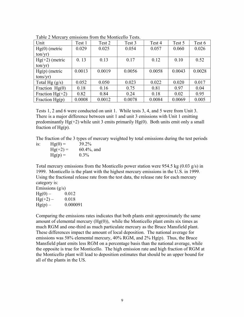
Table 2 Mercury emissions from the Monticello Tests. Unit Test 1 Test 2 Test 3 Test 4 Test 5 Test 6 Hg(0) (metric ton/yr)

0.029 0.025 0.054 0.057 0.060 0.026

Hg(+2) (metric ton/yr)

0. 13 0.13 0.17 0.12 0.10 0.52

Hg(p) (metric tons/yr)

0.0013 0.0019 0.0056 0.0058 0.0043 0.0028

Total Hg (g/s) 0.052 0.050 0.023 0.022 0.020 0.017 Fraction Hg(0) 0.18 0.16 0.75 0.81 0.97 0.04 Fraction Hg(+2) 0.82 0.84 0.24 0.18 0.02 0.95 Fraction Hg(p) 0.0008 0.0012 0.0078 0.0084 0.0069 0.005 Tests 1, 2 and 6 were conducted on unit 1. While tests 3, 4, and 5 were from Unit 3. There is a major difference between unit 1 and unit 3 emissions with Unit 1 emitting predominantly Hg(+2) while unit 3 emits primarily Hg(0). Both units emit only a small fraction of Hg(p). The fraction of the 3 types of mercury weighted by total emissions during the test periods is: Hg(0) = 39.2% Hg(+2) = 60.4%, and Hg(p) = 0.3% Total mercury emissions from the Monticello power station were 954.5 kg (0.03 g/s) in 1999. Monticello is the plant with the highest mercury emissions in the U.S. in 1999. Using the fractional release rate from the test data, the release rate for each mercury category is: Emissions (g/s) Hg(0) – 0.012 Hg(+2) – 0.018 Hg(p) – 0.000091 Comparing the emissions rates indicates that both plants emit approximately the same amount of elemental mercury (Hg(0)), while the Monticello plant emits six times as much RGM and one-third as much particulate mercury as the Bruce Mansfield plant. These differences impact the amount of local deposition. The national average for emissions was 58% elemental mercury, 40% RGM, and 2% Hg(p). Thus, the Bruce Mansfield plant emits less RGM on a percentage basis than the national average, while the opposite is true for Monticello. The high emission rate and high fraction of RGM at the Monticello plant will lead to deposition estimates that should be an upper bound for all of the plants in the US.

9

3.2 Meteorological Data The Bruce Mansfield plant is located in Shippingport, PA about 25 miles northwest of Pittsburgh, PA. Meteorological data from the year 1990 were selected for use in the evaluation of deposition. Weather is variable, from year to year, and will change deposition amounts and patterns. The year 1990 was chosen for illustrative purposes and not with the intent of predicting deposition that occurred in a particular year. Data from 1999, the year of the emissions data, would have been preferable, but were not available. In 1990, the winds were primarily out of the south and west as displayed in the windrose, Figure 1. The wind during precipitation events was more uniformly distributed in all directions, Figure 2, with the exception of the Northeast. Rainfall was measured in 9.1% of the hours in the year. A total of 133 cm of precipitation was measured in 1990. The average wind velocity was 8.8 knots. However, during rainfall events, the winds were generally light. The Monticello plant is located in Monticello, TX about 9 miles south west of Mount Pleasant TX and about 60 miles east and north of Dallas, TX. Meteorological data from 1990 taken in Abilene was used as the basis for deposition modeling. The wind is almost always from due north or south, predominantly from the south (25% of the time), Figure 3. Approximately 10% of the time the wind is out of the north. In contrast, precipitation events occur most frequently when the wind is out of the north, Figure 4. Southeasterly winds also account for substantial rainfall. Rainfall occurred approximately 4% of the time with a total amount of 80 cm.

10

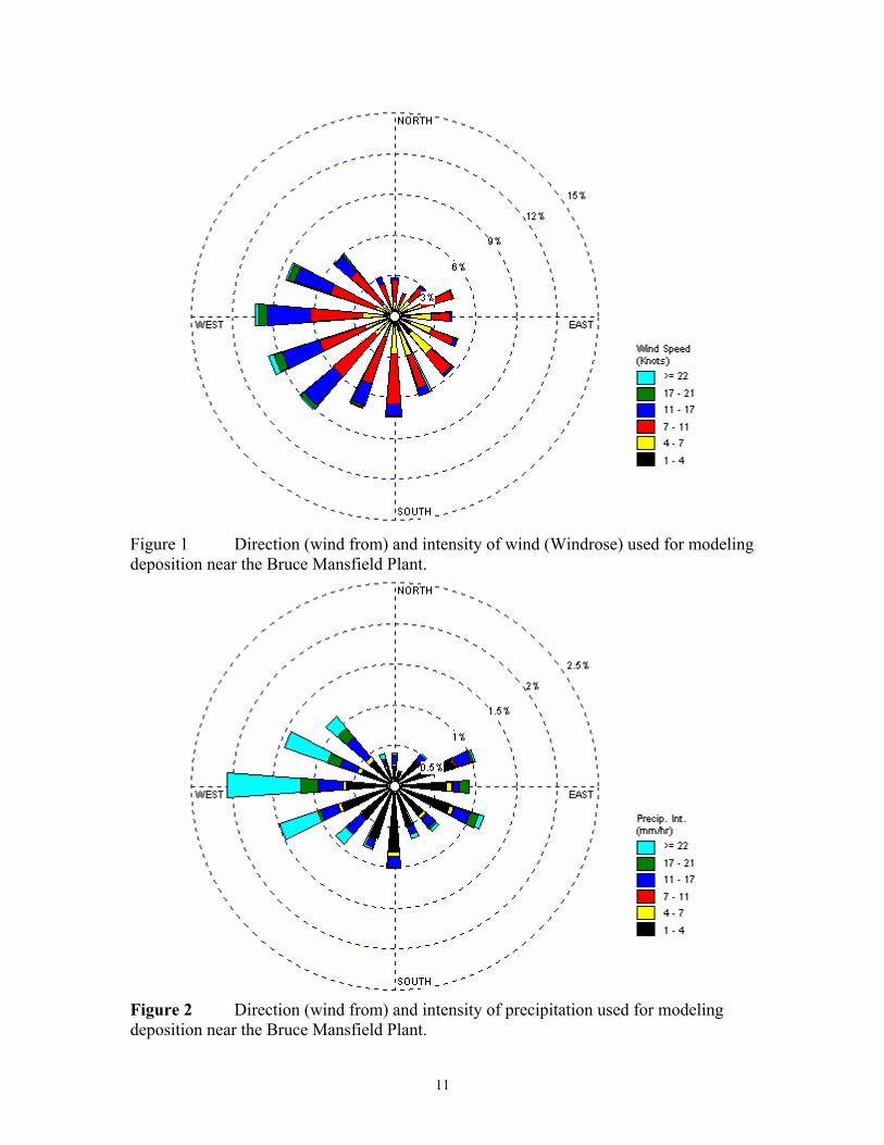
Figure 1 Direction (wind from) and intensity of wind (Windrose) used for modeling deposition near the Bruce Mansfield Plant.

Figure 2 Direction (wind from) and intensity of precipitation used for modeling deposition near the Bruce Mansfield Plant.

11

Figure 3 Direction (wind from) and intensity of wind (Windrose) used for

modeling deposition near the Monticello power plant.

Figure 4 Precipitation Intensity and Direction (wind from) used for modeling deposition around the Monticello Power Plant.

12

3.3 Deposition Parameters Once emitted from the stack, mercury can deposit through wet or dry processes. Wet deposition occurs when mercury is accumulated in precipitation and then deposited with the precipitation. The amount of accumulation depends strongly on the type of mercury. Particulate mercury is readily removed by rain. Reactive gaseous mercury and the compounds it forms also have a high solubility in water and are readily incorporated into precipitation. Elemental mercury has a low solubility and does not tend to accumulate in rain to the degree as the other two types of mercury. Dry deposition also depends strongly on the type of mercury. In general, reactive gaseous mercury deposits at a higher rate per unit mass than particulate mercury or elemental mercury due to its highr chemical reactivity with particulate surfaces. In this analysis, the distribution of mercury between the three different conditions was assumed to equal that measured at the exhaust stack. It is recognized that this is a simplification of reality, as the ratio when emitted from the stack is likely to change as the distance from the stack increases due to atmospheric chemical reactions. 3.3.1 Wet Deposition ISCST models wet deposition using rainfall intensity and an empirical parameter known as the scavenging coefficient. The total flux to be deposited is the product of the scavenging ratio multiplied by the concentration integrated over the vertical dimension. The scavenging ratio is composed of two parameters, precipitation intensity (mm/hr) and a scavenging coefficient (s-mm/hr)-1. The scavenging coefficient depends on the characteristics of the pollutant (e.g., solubility and reactivity for gases, size distribution for particles) as well as the nature of the precipitation (e.g., liquid or frozen). Scavenging rate coefficients are expected to be approximately 1/3 smaller for frozen precipitation. Direct measurements of scavenging parameters for mercury are not available. However, estimates of a washout ratio, (concentration in precipitation to concentration in air), were provided in the EPA’s report to Congress (1998c). The washout ratio can be related to the scavenging coefficient used in ISCST. The washout ratio for reactive gaseous mercury is 1.6 106, while the ratio for elemental mercury is 1200. The large difference reflects the much higher solubility of reactive gaseous mercury. Using these values, the scavenging coefficient was calculated as 2.5 10-4 (s-mm/hr)-1 for reactive gaseous mercury and 3.310-7 (s-mm/hr) -1 for elemental mercury. Particle deposition rates depend on the particle size. In this study, particle size distributions obtained by Landis were used for estimating deposition (Landis, 1998). In measurement of particles over Lake Michigan, two size categories were determined, coarse and fine. The fine fraction is believed to result from combustion processes and accounted for 70% of the surface area of all particles. The particle diameter for the fine fraction was 0.68 µm. The coarse fraction particle median diameter was 3.5 µm. The scavenging coefficient for 0.68 µm particles was taken as 7 10-5 (s-mm/hr)-1 while for

13

3.5 µm particles it increases to 2.8 10-4 (s-mm/hr)-1. Wet deposition parameters are summarized in Table 3. Table 3: Wet Deposition Parameters. Form of Mercury Liquid Scavenging

Coefficient (s-mm/hr)-1 Frozen Scavenging Coefficient (s-mm/hr)-1

Hg(0) 3.310-7 1.0 10-7 Hg(+2) 2.5 10-4 5.0 10-5 Hg(p) 0.68 µm 7.0 10-5 2.0 10-5 Hg(p) 3.5 µm 2.8 10-4 9.0 10-5

14

3.3.2 Dry Deposition Parameters Dry deposition is frequently modeled using a deposition velocity. In general, the dry deposition velocity is a function of ground cover (e.g. grass, forests, water, etc.) and weather conditions. The total deposition flux is the product of the deposition velocity and the concentration at the ground surface. In the EPA Report to Congress on Mercury, dry deposition velocities were calculated over a range of conditions and the average deposition velocity for elemental mercury was 0.06 cm/s while for reactive gaseous mercury the average value is 2.9 cm/s (EPA, 1998c). Particle deposition also depends on the size of the particles, with larger particles falling at their gravitational settling velocity which is controlled by their size and friction factors and smaller particles at a slower rate. Landis (Landis, 1998) developed a model for predicting deposition velocity as a function of particle size, Figure 5.

Figure 5 Dry deposition velocity as a function of particle size (from Landis, 1998).

Landis also calculated dry deposition rates for various size particles under different conditions and obtained average values of 0.09 cm/s for fine particles (0.68 µm) and 0.45 cm/s for coarse particles (3.5 µm) (Landis, 1998). Dry deposition parameters are summarized in Table 4.

15

Table 4 Dry Deposition Parameters Form of Mercury Dry Deposition Velocity (cm/s) Hg(0) 0.06 Hg(+2) 2.9 Hg(p) 0.68 µm 0.09 Hg(p) 3.5 µm 0.45 4.4 Coal Plant Parameters In order to run, ISCST, the stack height, stack exhaust temperature, and stack exit diameter and velocity are required. Stack exhaust temperatures were measured as part of the information collection request. The other data were selected to be consistent with the values used for large coal fired power plants in the EPA’s report to Congress (EPA, 1998c). Table 5 contains the values used in modeling deposition at both power plants. Table 5 Coal Plant Parameters Parameter Value Stack Height (m) 223 Stack Diameter (m) 7 Exit Velocity (m/s) 21.6 Monticello Exhaust Temperature (oK) 379 Bruce Mansfield Exhaust Temperature (oK) 326

16

4.0 Local Deposition Modeling Results The data presented in Chapter 4 were used to predict the amount of local deposition around the Bruce Mansfield and Monticello power plants. In the simulations the concentration of mercury in air (ng/m3), wet deposition (µg/m2/yr) and dry deposition (µg/m2/yr) were computed on a 1 km grid centered around the plant. Air concentrations were available in terms of a yearly average value as well as peak values over a 24 hour period. Simulations were carried out for a minimum of 25 km in the downwind direction. Local deposition modeling was performed to indicate the increase in concentrations and deposition over natural background. Concentrations of mercury in air have been determined from a number of locations. Typical values are around 1 – 4 ng/m3 in rural areas and 10 – 50 ng/m3 in urban areas (Landis, 1988). In EPA’s report to Congress (EPA, 1998 c) a value of 1.7 ng/m3 was the average mercury level away from sources. Wet deposition is being measured throughout the country through the Mercury Deposition Network. Deposition rates range from 5 – 25 ug/m2/yr. In western Pennsylvania between 1998 and 2001, the range is between 8 – 12 ug/m2/yr. In eastern Texas during that time period, the range is 10 –16 ug/m2/yr. Dry deposition is not well understood but estimates indicate that it should be in the range of 50 to 100% of wet deposition. For a comparison basis, this study will use an air concentration value of 1.7 ng/m3, the value used in the EPA Report to Congress for rural areas; wet deposition of 10 ug/m2/yr, based on Mercury Deposition Network Data; dry deposition of 10 ug/m2/yr; based on average literature estimates; and a total deposition of 20 ug/m2/yr as typical background levels. 4.1 Bruce Mansfield Local Deposition Results Local deposition modeling was performed for the Bruce Mansfield plant using the data presented in section 4. Figure 1 presents the predicted yearly average total mercury concentration data around the plant. The predominant form of mercury emitted from the Bruce Mansfield plant is Hg(0) and it constitutes approximately 80% of the total mercury. Ground-level concentrations peak to the east and northeast of the plant, consistent with the prevailing winds, Figure 1. The peak value is 0.015 ng/m3, less than 1% of the expected background concentration, 1.7 ng/m3. Although yearly average concentrations are low, it must be kept in mind that these concentrations represent the ground-level concentrations. Therefore, values near the centerline of the plume will be higher. The maximum daily average ground-level concentration was 0.13 ng/m3, approximately 8% of the expected background. This indicates that even in the immediate vicinity of a power plant, the ground-level concentrations are only a small fraction of background levels.

17

Figure 6 Predicted total mercury ground-level air concentrations (ng/m3) around the Bruce Mansfield Power Plant (Plant located at (0,0)).

Away from sources, the amount of reactive gaseous mercury is typically 1 – 3% of the total amount of mercury. Thus, background values of RGM are expected to range between 0.02 and 0.05 ng/m3. Near the Bruce Mansfield Plant, in the region depicted in Figure 6, predicted RGM values average 0.0025 ng/m3, approximately 1/10 of the background level. Figure 7 presents the predicted total wet deposition of mercury around the Bruce Mansfield Power Plant. Due to the different deposition characteristics although only 20% of the mercury emitted is in the form of RGM (Hg + 2), 84% of the deposited mercury is RGM. In contrast to the concentration plume, the wet deposition is located almost uniformly around the plant with excess deposition of 5 ug/m2/yr extending no more than 10 km from the plant. Deposition is primarily along the east-west plane consistent with the predominant winds during precipitation, Figure 2.

18

Figure 7 Total predicted wet deposition around the Bruce Mansfield Power Plant.

The estimated background wet deposition rate is 10 ug/m2/yr, thus a region near the plant is predicted to have deposition 2 to 3 times theassumed background wet deposition. Figure 8 presents the predicted mercury dry deposition pattern around the Bruce Mansfield plant. Again, due to the different deposition velocities, RGM contributes approximately 85% of the total deposition even though it is only 20% of emissions. The deposition pattern reflects the concentration pattern and peaks to the east of the facility consistent with the prevailing winds. Total deposition rates are much lower than for wet deposition, but they are distributed over a much greater area. The fact that the peak is away from the plant results from the emission at elevated temperature and height.

19

Figure 8 Total predicted mercury dry deposition around the Bruce Mansfield Power Plant.

Figure 9 shows the total predicted mercury deposition around the Bruce Mansfield Power Plant. The addition of the dry deposition marginally increases the 5 ug/m2/yr contour of the wet deposition towards the east, but leaves the general pattern unchanged.

20

Figure 9 Total predicted deposition around the Bruce Mansfield Power Plant.

Table 6 summarizes the average yearly maximum concentration and deposition amounts resulting from the model predictions. The maximum yearly average concentrations for all three species are well below expected background levels. Wet deposition peaks near the source, the location (0,1000) is the first computational point. Use of the steady-state Gaussian plume model in ISCST near the source may not be accurate. However, a prediction of deposition of 91 ug/m2/yr indicates that high deposition will occur near the source under precipitation conditions due to washout. Table 7 summarizes the total mass deposited and the average deposition rate over the modeled area for each of the three forms of mercury. The total mass deposited over the modeled domain is predicted to 8800 grams or 1.9% of the total emitted. This indicates that the vast majority of mercury emitted from the Bruce Mansfield plant is not deposited within 30 km of the plant and enters the global mercury cycle. In the emissions, elemental mercury accounts for 78.5% of the mass, RGM accounts for 19.7% and particulate mercury accounts for 1.8%. In the deposition, RGM accounts for 84% of the

21

total deposition, elemental mercury accounts for 11% and particulate mercury accounts for 5%. The higher relative deposition rates of RGM and particulate mercury reflect the higher values for their deposition parameters. Their fractional deposition rate (mass deposited over the modeled domain divided by the mass emitted from the plant) was around 6%, while less than 0.3% of the elemental mercury deposited locally. Although, the peak deposition rates are much higher for wet than dry deposition, the total mass deposited by each mechanism is approximately the same. Therefore, over the area of the modeled domain, the average deposition rates for wet and dry deposition are similar. The area average deposition rate, 3.0 ug/m2/yr is approximately 15% of that expected from background (20 ug/m2/yr). This number, 15%, is used in the risk assessment to evaluate the impacts of local mercury deposition on health risk. Around the plant, there is an area of approximately 50 km2 which receives an average deposition rate of 20 ug/m2/yr. In this region, deposition is doubled over background and this value will be used to examine an upper bound on the potential increases in risk due to local deposition of mercury.

Table 6: Bruce Mansfield Plant yearly average maximum concentration and deposition values. Hg(0) Hg(+2) Hg(p) Location (m,m) Particulate (Hgp) Concentration (ng/m3) 2.9 10-4 (3000,3000) Wet Deposition (µg/m2/yr) 3.4 (0,1000) Dry Deposition (µg/m2/yr) 0.15 (14,000,5000) Reactive (RGM) Concentration (ng/m3) 3.3 10-2 (3000,3000) Wet Deposition (µg/m2/yr) 91 (0,1000) Dry Deposition (µg/m2/yr) 3.4 (3000,3000) Elemental (Hg(0)) Concentration (ng/m3) 1.33 10-1 (3000,3000) Wet Deposition (µg/m2/yr) 0.84 (-1000,0) Dry Deposition (µg/m2/yr) 0.24 (3000,3000)

22

Table 7: Bruce Mansfield Mercury Deposition summary. Hg(0) Hg(+2) Hg(p) Total Hg Total Mass deposited BRMANHGP BRMANRGM BRMANHG0 Wet deposition (gms) 646 3808 156 4610 Dry deposition (gms) 300 3559 306 4165 Total deposition (gms) 946 7367 462 8775 Avg deposition rate Avg Wet Deposition (µg/m2/yr)

0.026 1.5 0.063 1.6

Avg Dry Deposition (µg/m2/yr)

0.012 1.4 0.012 1.4

Avg Total Deposition 0.038 2.9 0.075 3.0 Fractional Deposition Fraction of Wet Deposition to Emissions

1.9 10-3 0.034 0.02 0.01

Fraction of Dry Deposition to Emissions

8.9 10-4 0.031 0.039 0.009

Fraction of Total Deposition to Emissions

2.79 10-3 0.065 0.059 0.019

23

4.2 Monticello Deposition Local deposition modeling was performed for the Monticello plant using the data presented in section 4. The Monticello plant emitted approximately twice as much mercury as the Bruce Mansfield plant and had the highest total emissions in the U.S. for 1999. In addition, it emits over 60% RGM, thus local deposition is expected to be among the highest of all U.S. plants. Figure 10 presents the predicted yearly average ground-level total mercury concentration around the plant. Concentrations peak to the north of the plant consistent with the prevailing southerly winds, Figure 3. The peak value is 0.04 ng/m3, less than 3% of the expected background concentration, 1.7 ng/m3. However, the amount of RGM is 0.022 ng/m3 which is approximately the same as the expected background level of RGM. The maximum daily average concentration was 0.58 ng/m3, approximately 34% of the expected background. This indicates that even in the immediate vicinity of the power plant with the largest emissions in the US, the increase in air concentrations are only a fraction of background levels.

-20000 -10000 0 10000 20000 30000Distance from source (m)

-20000

-15000

-10000

-5000

0

5000

10000

15000

20000

25000

30000

Dis

tanc

e fr

om s

ourc

e (m

)

Monticello PlantTotal Mercury Ground-levelConcentration (ng/m^3)

Figure 10 Predicted ground-level total mercury air concentrations (ng/m3) around the Monticello Power Plant (Plant located at (0,0)).

24

Figure 11 presents the predicted total wet deposition of mercury around the Monticello Power Plant. Over 98% of the deposition arises from reactive gaseous mercury. This is due to the large fraction of RGM (60%) in the emissions and the large deposition parameters relative to elemental mercury. Due to the wind flow being almost exclusively in the north-south direction, the wet deposition is located along this axis. The large amount of RGM in the emissions leads to high predicted deposition rates. Wet deposition is predicted to be greater than 40 ug/m2/yr (4 times wet deposition background) for a distance of five kilometers from the plant in both the north and south directions. The predicted region with excess deposition of 5 ug/m2/yr extends more than 50 km along the north-south axis.

-20000 -10000 0 10000 20000 30000

Distance from source (m)

-20000

-15000

-10000

-5000

0

5000

10000

15000

20000

25000

30000

Dist

ance

from

sour

ce (m

)

Monticello Power StationTotal mercury deposition (ug/m^2/yr)

Figure 11 Total predicted mercury wet deposition (ug/m2/yr) around the Monticello Power Plant

25

Figure 12 presents the predicted dry deposition pattern around the Monticello power plant. Again, due to the different dry deposition velocities, RGM contributes approximately 98% of the total deposition even though it is only 60% of emissions. The deposition pattern peaks to the north of the facility consistent with the prevailing winds. Total deposition rates are in excess of the estimated background dry deposition rate of 10 ug/m2/yr for more than 30 km from the plant. Subsequent modeling showed that the region of dry deposition in excess of 10 ug/m2/yr was contained within 50 km of the plant. The fact that the peak is away from the plant results from the emission at elevated temperature and height.

-20000 -10000 0 10000 20000 30000

Distance from Source (m)

-20000

-15000

-10000

-5000

0

5000

10000

15000

20000

25000

30000

Dis

tanc

e fr

om S

ourc

e (m

)

Monticello Power StationTotal Dry deposition (ug/m^2/yr)

Figure 12 Total predicted mercury dry deposition (ug/m2/yr) around the Monticello Power Plant.

26

Figure 13 shows the total predicted deposition around the Monticello power plant. The deposition is peaked along the north-south axis, which is the direction of wind flow.

Figure 13 Predicted total mercury deposition (ug/m2/yr) around the Monticello Power Plant.

Table 8 summarizes the total mass deposited and the average deposition rate over the modeled area around the Monticello plant for each of the three forms of mercury. The total mass deposited over the modeled domain is predicted to be 23400 grams or 2.5% of the total emitted. Increasing the distance to a 50 km radius around the plant did not change the predicted wet deposition. However, the dry deposition mass increased by a factor of 3 to 29100g. The total deposition within 50 km of the plant was 40100 grams, 4.2% of the total emitted. This indicates that the vast majority of mercury emitted from the Monticello plant is not deposited within 50 km of the plant and enters the global mercury cycle. In the emissions, elemental mercury accounts for 40% of the mass, RGM accounts for 60% and particulate mercury accounts for 0.3%. In the deposition, RGM is responsible for 98.7% of the total deposition, elemental mercury accounts for 1.1% and particulate mercury accounts for 0.2%. Their fractional deposition rate (mass deposited over the modeled domain divided by the mass emitted from the plant) was around 4%, while less than 0.07% of the elemental mercury deposited locally. Although, the peak deposition rates are much higher for wet than dry deposition, the total mass deposited by each mechanism is approximately the same. Increasing the modeled area from 30 km downwind of the plant to 50 km increased dry deposition by a factor of 3. Therefore,

27

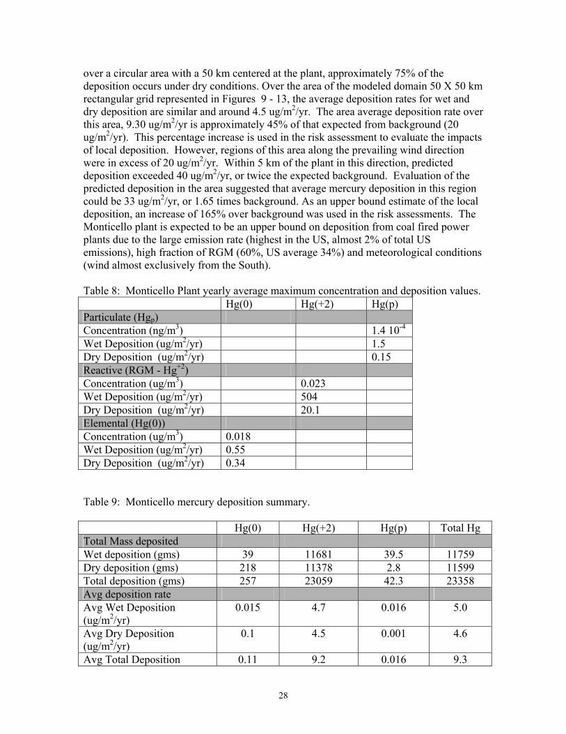
over a circular area with a 50 km centered at the plant, approximately 75% of the deposition occurs under dry conditions. Over the area of the modeled domain 50 X 50 km rectangular grid represented in Figures 9 - 13, the average deposition rates for wet and dry deposition are similar and around 4.5 ug/m2/yr. The area average deposition rate over this area, 9.30 ug/m2/yr is approximately 45% of that expected from background (20 ug/m2/yr). This percentage increase is used in the risk assessment to evaluate the impacts of local deposition. However, regions of this area along the prevailing wind direction were in excess of 20 ug/m2/yr. Within 5 km of the plant in this direction, predicted deposition exceeded 40 ug/m2/yr, or twice the expected background. Evaluation of the predicted deposition in the area suggested that average mercury deposition in this region could be 33 ug/m2/yr, or 1.65 times background. As an upper bound estimate of the local deposition, an increase of 165% over background was used in the risk assessments. The Monticello plant is expected to be an upper bound on deposition from coal fired power plants due to the large emission rate (highest in the US, almost 2% of total US emissions), high fraction of RGM (60%, US average 34%) and meteorological conditions (wind almost exclusively from the South). Table 8: Monticello Plant yearly average maximum concentration and deposition values. Hg(0) Hg(+2) Hg(p) Particulate (Hgp) Concentration (ng/m3) 1.4 10-4 Wet Deposition (ug/m2/yr) 1.5 Dry Deposition (ug/m2/yr) 0.15 Reactive (RGM - Hg+2) Concentration (ug/m3) 0.023 Wet Deposition (ug/m2/yr) 504 Dry Deposition (ug/m2/yr) 20.1 Elemental (Hg(0)) Concentration (ug/m3) 0.018 Wet Deposition (ug/m2/yr) 0.55 Dry Deposition (ug/m2/yr) 0.34 Table 9: Monticello mercury deposition summary. Hg(0) Hg(+2) Hg(p) Total Hg Total Mass deposited Wet deposition (gms) 39 11681 39.5 11759 Dry deposition (gms) 218 11378 2.8 11599 Total deposition (gms) 257 23059 42.3 23358 Avg deposition rate Avg Wet Deposition (ug/m2/yr)

0.015 4.7 0.016 5.0

Avg Dry Deposition (ug/m2/yr)

0.1 4.5 0.001 4.6

Avg Total Deposition 0.11 9.2 0.016 9.3

28

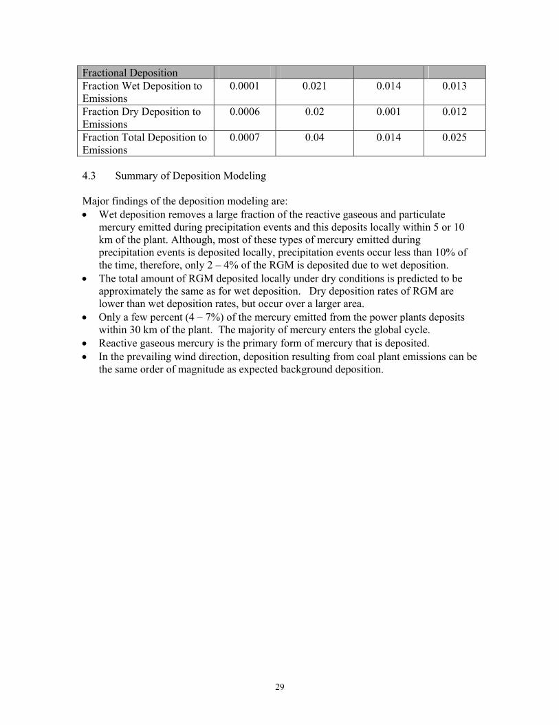
Fractional Deposition Fraction Wet Deposition to Emissions

0.0001 0.021 0.014 0.013

Fraction Dry Deposition to Emissions

0.0006 0.02 0.001 0.012

Fraction Total Deposition to Emissions

0.0007 0.04 0.014 0.025

4.3 Summary of Deposition Modeling Major findings of the deposition modeling are: • Wet deposition removes a large fraction of the reactive gaseous and particulate

mercury emitted during precipitation events and this deposits locally within 5 or 10 km of the plant. Although, most of these types of mercury emitted during precipitation events is deposited locally, precipitation events occur less than 10% of the time, therefore, only 2 – 4% of the RGM is deposited due to wet deposition.

• The total amount of RGM deposited locally under dry conditions is predicted to be approximately the same as for wet deposition. Dry deposition rates of RGM are lower than wet deposition rates, but occur over a larger area.

• Only a few percent (4 – 7%) of the mercury emitted from the power plants deposits within 30 km of the plant. The majority of mercury enters the global cycle.

• Reactive gaseous mercury is the primary form of mercury that is deposited. • In the prevailing wind direction, deposition resulting from coal plant emissions can be

the same order of magnitude as expected background deposition.

29

5.0 Risk Assessment The objective of this study is to quantify the impact of local mercury deposition from coal fired power plants on risks from fetal exposure through maternal consumption of fish. Based on the data collected in the 1999 EPA data collection request, we used the mercury emissions data from two power plants, Monticello approximately 60 miles east and north of Dallas, TX, and Bruce Mansfield in Shippingport, PA, as the basis for modeling local deposition. Both of these plants emitted substantial quantities of mercury and can serve as a basis for examining potential impacts of local deposition under high loadings. The Monticello plant has three coal-fired units and the combined emissions from this plant were the highest total mercury emissions of any plant in the country in 1999 and it emitted 1 ton of mercury, approximately 2% of the total amount emitted by all coal fired power plants in the U.S. The Bruce Mansfield plant’s 1999 emissions totaled 0.48 tons (approximately 1% of the U.S. total). Meteorological data for a one-year period was taken from nearby weather stations, Abilene airport which is approximately 150 miles from the Monticello site and Pittsburgh airport, which is approximately 25 miles from the Bruce Mansfield site. The Abilene data was chosen to represent the Monticello site because of the availability of hourly precipitation data. Wind data from Dallas/Fort Worth, approximately 60 miles west of the Monticello site and from Shreveport, La, approximately 60 miles east of the site showed the same pattern as in Abilene. Total precipitation amounts from these 3 sites are also similar. Future studies could use data from these sites, or from the plant to improve wind and weather predictions for the site. The risk assessment was performed for the general population in the vicinity of these power plants. In addition, particular concern is expressed for populations that consume high fractions of freshwater fish. These would include subsistence fishers and recreational fishers. This study quantifies the risk for the general population and subsistence fisher groups with and without the emissions from the plants. Without local deposition, the risk is calculated based on fish consumption patterns and typical values for Hg concentrations in fish, section 5.2. When local deposition is taken into account, it is assumed that an increase in deposition leads to a linearly proportional increase in Hg concentration in local fish (i.e., if deposition increases by 20%, Hg concentrations in fish increase by 20%). The risks are calculated for the base case (no local deposition) and two cases of increased deposition. The first uses the average increase over the 50 X 50 km local deposition modeled domain. The second uses the average increase over the region near the 5 – 10 km region around the plant characterized by high deposition. Values for the percentage increase for each case were presented in Section 4. In a site-specific risk assessment, an evaluation of the local water bodies in this region and the population that fishes these water bodies would be needed. If there are no large lakes near the plant, the ability of the local population ot The population risk is defined as the probability of having a chance of exhibiting any adverse neurological effect observed in the three epidemiology studies used to develop the dose response functions (DRF). The DRF correlates the risk with the biomarker of Hg concentration in hair, which is a function of the amount of Hg consumed through fish.

30

The population risk is obtained through summation over all individuals that comprise the population. The population risk is then obtained from the following equation. Population Risk = Σi (Ei * Ci * Hi* Ai* Pi) (1) Where: i = the index for each individual Ei = amount of fish eaten (g/d) Ci = mercury concentration in fish (ug Hg/g fish). Hi = conversion factor between mercury intake (Ei*Ci ug/d) and concentration in hair (ppm). Ai = fraction of the population that consumes Ei (g/d) of fish with a given (Ci) mercury concentration. Pi = probability of having an adverse effect from consuming (Ei*Ci ug Hg/d) at a given hair concentration of Hg. The probability of having an adverse effect, Pi, is obtained from a dose response function (DRF) that correlates exposure (dose) to the probability of having an adverse effect (response). The dose response function is discussed in detail in this section 5.5 of this report. In practice, people consume many different types of fish with varying concentrations of Hg. Dozens of studies have been performed to characterize mercury concentrations by fish species. To account for consumption of different fish species, equation (1) can be generalized as follows: Population Risk = Σi [(Σj Ei,j * Ci,j )* Hi* Ai* Pi] (2) Where Ei,j is the amount of fish species j consumed per day by individual i. Ci,j is the mercury concentration (µg/g) in fish species j consumed by individual i. In practice, the type and amount of fish consumed as well as the amount of mercury in each fish can not be tracked on a fish-by-fish basis for every individual. For this reason, statistical approaches based on Monte Carlo simulation are used to estimate the fraction of population that consumes various amounts of fish with different mercury levels is calculated. The exposure is converted to a concentration of Hg in hair. This is translated into a risk estimate by multiplying by the dose conversion factor that relates the probability of having an effect to the level of Hg in hair, section 5.3. Each of the variables: consumption: mercury concentration in fish; and correlation of consumption to mercury level in hair; are represented by a statistical distribution characterized by a mean and standard deviation. In each case, a log-normal distribution was assumed to be the most representative of the data.

31

5.1 Population Groups In this report, we have modeled the local deposition of mercury resulting from emissions at two power plants, Monticello and Bruce Mansfield. Particular concern is expressed for populations that consume high fractions of locally caught freshwater fish. These would include subsistence fishers and recreational fishers. The EPA in their guidance for conducting risk assessment from mercury exposure suggests that the reasonable maximum exposure (RME) rate of 25 g/d for recreational anglers with a central tendency exposure (CTE) of 8 g/d (EPA,1997). A consumption rate of 25 g/day represents the upper percentile of recreational anglers consuming freshwater fish (EPA 1997). The EPA guidance, Methodology for Deriving Ambient Water Quality Criteria (EPA 2000), uses a consumption rate of 17.5 g/day for determining ambient water quality criteria, which is considered to be protective of the general population and recreational fishers. This consumption rate represents the 90th percentile of freshwater and estuarine finfish and shellfish consumption by individuals age 18 or older (EPA, 2000), and was developed from an evaluation of more recent fish consumption patterns in the U.S. than the consumption rate used to estimate the RME. Several detailed studies of subsistence fisher groups have been made. For the purposes of this report, the subsistence fisher population in Texas near the Monticello plant will be based on the study conducted in the Savannah River in South Carolina (Burger, 1998). The consumption data from this study asserts a mean consumption rate of 67 g/d was used to develop a log-normal distribution for consumption of fresh water fish by subsistence fishers. The resulting log-normal distribution was used as a basis for estimating risks to subsistence fisher populations near the Monticello plant. This consumption rate is much higher than the EPA suggested RME of 25 g/d. For the Bruce Mansfield plant, the study by Stern in New Jersey that had a log normal distribution with a mean consumption rate of 41 g/d and a standard deviation of 34.2 was used. 5.2 Consumption by Fish Species For the two power plant regions, it is assumed that the general populations consume both freshwater and marine fish. The fraction of freshwater fish consumed in each region is defined by a normal distribution with a mean consumption rate and standard deviation. The fraction of marine fish is calculated such that the sum of fractions of freshwater and marine fish consumption equals 1. National data suggests that 83% of fish consumed in this country is saltwater fish while the remainder is freshwater fish. For the subsistence fishers example, it is assumed that all fish consumed is caught locally and therefore freshwater fish. 5.3 Conversion of Consumption Rate to Hair Hg levels Lipfert (Lipfert, 1997) presented a table comparing mercury consumption with mean level of Hg in hair collected from 18 studies worldwide. The data were plotted on a log-log plot of consumption (ug/kg/d) vs. hair Hg (ppm) and a linear regression was performed with a best fit slope of 0.77. This indicates that the hair mercury levels

32

increase at a slower rate than consumption. The data from this report were analyzed and the mean conversion factor from consumption (ug/d) to hair Hg (ppm) was 0.11 with a standard deviation of 0.05. To incorporate the finding that the conversion factor for consumption to hair Hg levels decreases with increasing consumption, the SPSS statistical package was used to develop the correlation (-0.516) between consumption rate and hair Hg level. This forced high consumption rate samples to have lower consumption to hair conversion factors in the Monte Carlo analysis. 5.4 Increase in Fish Mercury levels due to local deposition In assessing the impacts of local deposition of Hg from coal power plants on Hg levels in fish, we are most interested in local freshwater fish consumed by the population. Marine fish such as tuna, swordfish, shellfish, etc., will be largely unaffected by changes in U.S. emissions in Hg. This assertion is based on the fact that slightly less than 1% of the global total Hg emissions results from coal fired plants in the U.S. Therefore, it is likely that completely stopping Hg emissions from coal plants in the U.S. would lead to less than a 1% decrease in Hg levels in marine fish. In this study, the Hg level in marine fish is held constant. For freshwater fish, an assumption is made that an increase in deposition leads to a linear increase in mercury levels in fish. At both plants, the background deposition of mercury was assumed to be 20 ug/m2/yr. This included both wet and dry deposition rates that are assumed to be equal at 10 ug/m2/yr. Measurements conducted through the Mercury Deposition Network (http://nadp.sws.uiuc.edu/mdn/) indicate that wet deposition at the station nearest to the Monticello site ranged from 10.5 – 15.5 ug/m2/yr between 1998 and 2001, while deposition ranged from 9.1 – 9.8 ug/m2/yr at the location nearest the Bruce Mansfield site during that period. Dry deposition rates are not well known but are believed to be approximately the same order of magnitude as wet deposition rates. 5.5 Dose Response Function The basis for determining the dose response function for Hg exposure is three separate epidemiological studies conducted in the Seychelles, Faroe Islands, and New Zealand during the 1990’s and discussed in detail in the National Academy of Sciences report (NAS, 2000). These epidemiological studies were conducted on populations that had high consumption of seafood and therefore, high mercury levels in hair and other biomarkers. They all evaluated the impacts of Hg exposure to children and the measures of impact involved a series of tests of cognitive abilities (copying errors, language skills, etc) in terms of a benchmark dose (BMD). The benchmark dose is the estimated dose corresponding to a specified incremental percentage of poor performers in a given test over and above background. EPA has taken the specified increment to be 5%. From a distribution of responses to a given test, the 5% with the poorest response are defined as being clinically subnormal. After exposure of a population to the BMD, an additional 5% of the population would score at the clinically subnormal level defined by the unexposed population. A second parameter, Bench Mark Dose Lower Limit (BMDL) is defined as the level at which there is 95% confidence that an effect will not occur. Thus, the benchmark dose is the mean value at which an effect may occur, and the BMDL is the 95% lower confidence limit of the BMD. Thus, with the assumption of a normal

33

distribution, the BMD and BMDL can be used to estimate the standard deviation in the BMD. In this study, Monte Carlo sampling among the 16 BMDs and their associated distributions was performed and the resulting pooled BMD and the pooled distribution results in a dose response function (DRF) that is a measure of the probability of a 5% increase over background in observing an effect at a given exposure level. In the three studies, a total of sixteen possible adverse effects were evaluated and a benchmark dose was determined for each. The frequency distribution obtained by pooling BMDs constitutes a dose-response function, where the "response" is the probability of having a 5% chance of experiencing any of the various health endpoints that were pooled. The details of this process and the advantages of using pooled data to estimate the dose response function were reported in Sullivan, 2001. There is no universally accepted approach to pool the dose response effects from different studies. Even within a single study, there is no universally accepted way to weigh different effects (NAS, 2000). In an attempt to examine a range of possible effects, three weighting approaches were used for combining the response from the three studies: straight average, average of the logarithms, and average of the reciprocals. The straight average approach tends to emphasize the data that suggest high values of hair Hg are needed to see an effect (i.e. the Seychelles study where effects were not seen), the average of the reciprocals tends to emphasize data that suggest lower values of hair Hg are indicative of an effect (New Zealand study). The latter method is consistent with the way that each BMD is derived, i.e., in terms of the reciprocal of the regression slope. The 16 estimates of benchmark dose from the three studies were pooled using Monte Carlo simulation to accomplish the averaging using the three different weighting procedures. Each study was weighted by the square rot of the participants in the study divided by the sum of the square roots of the participants in each study. Note that the mean of all three estimates is higher than the EPA “reference dose” (11 ppm). The overall dose response functions (DRF) are shown in Figure 14. In this case, the dose response function is a measure of the probability of having an effect and is not related to the severity of the effect. When a straight average is used for the 16 BMDs, a very steep DRF is obtained (right-most curve) with less than 1% probability of having a 5% chance of an effect below about 28 ppm hair Hg. This is consistent with the results of the Seychelles studies and with most studies on adults. Using the reciprocal of each BMD gives a different DRF that is very steep and has less than 1% probability below 18 ppm Hair Hg. The third curve was obtained using the logarithm of each of the 16 BMDs. The logarithmic weighting suggests a 1% probability at 14 ppm Hair Hg. The logarithmic curve does not have a physical basis, but it does prevent the highest predicted risks at the lowest exposure levels and for this reason it was used to estimate risks in the remainder of this report.

34

Pooled BMD

1.E-05

1.E-04

1.E-03

1.E-02

1.E-01

1.E+00

1 10 100

Hair Hg (ppm)

Pro

babi

lity

of O

bser

ving

an

Effe

ct

Log Weighting

Reciprocal Weighting

Average Weighting

Figure 14: Pooled Benchmark Dose Response Functions for reciprocal, log, and arithmetic weighting.

35

Table 10 Benchmark Dose estimates

from the NAS Report on Methylmercury (values expressed as ppm hair Hg [p. 284])

BMD BMDL std deviation Seychelles study (weight = .37) Bender copying errors 100* 25 45.6 Child behavior checklist 21 17 2.4 McCarthy general cognitive 100* 23 46.8 Preschool language scale 100* 23 46.8 WJ applied problems 100* 22 47.4 WJ Letter/Word recognition 100* 22 47.4

• * = values > 100, assumed upper limit of 100.

Faroes study (weight = .44) Finger tapping 20 12 4.8 CPT reaction time 17 10 4.2 Bender copying errors 28 15 7.9 Boston naming test 15 10 3.0 CVLT:delayed recall 27 14 7.9 New Zealand study (weight= 0.19) TOLD language development 12 6 3.6 WISC-R:PIQ 12 6 3.6 WISC-R:FSIQ 13 6 4.2 McCarthy perceptual 8 4 2.4 McCarthy motor test 13 6 4.2

weighted mean BMDs (ppm hair Hg) weight mean std deviation linear 43.2 6.5 log 31.3 10.9 reciprocal 22.0 1.8

36

6.0 Risk Assessment Test Cases and Results The deposition modeling results in the previous section were used to estimate the increased deposition that might occur from emissions from the Bruce Mansfield and Monticello power plants. Assuming that concentrations of mercury in fish are linearly proportional to mercury deposition, an estimate of the increase in risk to the local population due to mercury emissions can be made. Recent studies suggest that this is likely to be a conservative upper bound on increases in mercury concentration. A study by Bucholtz, 2002 did not find a correlation between mercury content in fish and deposition. Bucholtz did find a statistically valid correlation between anthropogenic sources and mercury levels in fish. There results showed that a 10% decrease in local sources would lead to a 0.6% decrease in fish mercury content. A USGS study suggests that the formation of methyl mercury increases logarithmically with total loading (Krabbenhoft, 1999). However, the authors acknowledge that the data they collected are insufficient to rule out the possibility that at low mercury loadings the relationship between deposition and methyl mercury production may be linear. The risk assessments performed for this analysis include three different test cases for each plant and two population groups, general population and subsistence fishers that consume only locally caught fish. For the general population, a unique fraction of consumption of local fish was used based on data for the region. The population near the Bruce Mansfield plant consumes 17% locally caught fish, similar to the average value in the northeast and the population near the Monticello plant consumes 22% locally caught fish, similar to the average value for the Southeast of the United States (Jacobs, 1998). There is a special concern pertaining to subsistence fishers or recreational anglers that consume large amounts of freshwater fish. These groups of people represent the high exposure cases that form the tail of the distribution of the general population. The actual risk to these groups will be highly variable and location specific. Therefore, the examples provided are intended to show the possible effects on subsistence fishers. For subsistence fisher populations two different consumption patterns were selected. For the population, near the Bruce Mansfield plant, consumption was based on data collected by Stern for women of child bearing age in New Jersey (Stern, 1996). For the population near the Monticello plant, subsistence fisher consumption rates were based on values obtained for a study along the Savannah River (Burger, 1998, 1999, 2001). While these consumption data are not an exact match for the locations under study, they are believed to be useful for illustrative purposes. Subsistence fishers that consume only locally caught fish are expected to be a small part of the total population (less than 1%). Table 11 summarizes the 12 test cases. The column on the increase in mercury deposition due to emission from coal fired power plants is based on the model results presented in Section 5.

37

Table 11: Risk Assessment Test Cases Plant Marine

Fish Local Fish

Increase in Mercury Deposition Due to Emission from Coal Plants (% of base case)

Mercury Levels in Local Fish (% of base case)

Bruce Mansfield Yes Yes 0 Base (100 %) Bruce Mansfield Local Region Yes Yes 15 115 Bruce Mansfield Near Plant Yes Yes 100 200 Bruce Mansfield No Yes 0 Base (100 %) Bruce Mansfield Local Region No Yes 15 115 Bruce Mansfield Near Plant No Yes 100 200 Monticello Yes Yes 0 Base (100 %) Monticello Yes Yes 46.5 146.5 Monticello Yes Yes 165 265 Monticello No Yes 0 Base (100 %) Monticello No Yes 46.5 146.5 Monticello No Yes 265 265 Table 12 summarizes key fish consumption and risk assessment parameters discussed in Section 5. The table provides the base case level. Therefore, if the plant emissions double local deposition, the fish concentration of mercury would be similarly doubled and the risks computed. The consumption rates and fish mercury content in Table 12 are mean values and their associated standard deviation. For the Monte Carlo analysis, a log-normal distribution of the data was assumed using these paramaters. It should be noted that for subsistence fishers, the consumption rates of locally caught fish far exceeds the EPA’s suggested reasonable maximum exposure of 25 g/d. Table 12: Key parameters for fish consumption and uptake used in risk assessments. Mean

Hg (ppm)*

Mean Consumption (g/d)*

Percentage of Freshwater Fish: General Population

Percentage of Saltwater Fish: General Population

Percentage of Freshwater Fish: Subsistence Fisher Population

Percentage of Saltwater Fish: Subsistence Fisher Population

US Average

0.21 (0.15)

18 (37.3) N/A N/A N/A N/A

Near Bruce Mansfield

0.41 (0.82)

41 (32.5) 17 83 100 0

Near Monticello

0.53 (0.47)

76.8 (67.6) 22 78 100 0

.* Numbers in parenthesis are the standard deviations for the distributions used in Monte Carlo analysis.

38

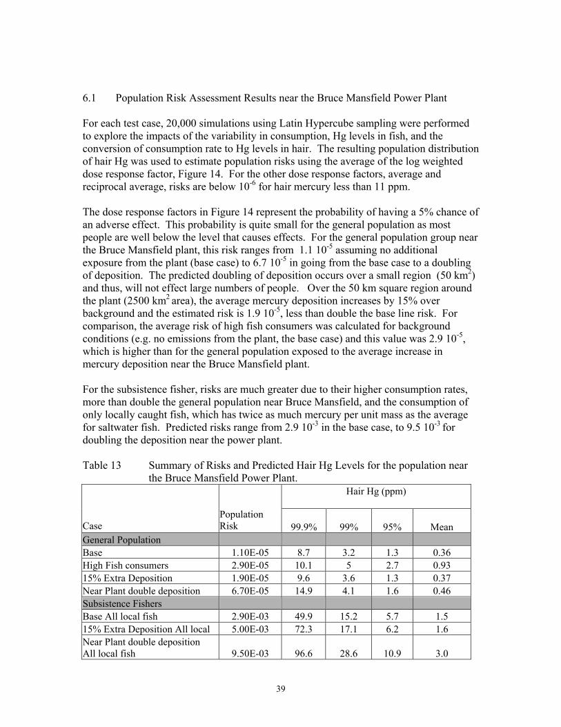
6.1 Population Risk Assessment Results near the Bruce Mansfield Power Plant For each test case, 20,000 simulations using Latin Hypercube sampling were performed to explore the impacts of the variability in consumption, Hg levels in fish, and the conversion of consumption rate to Hg levels in hair. The resulting population distribution of hair Hg was used to estimate population risks using the average of the log weighted dose response factor, Figure 14. For the other dose response factors, average and reciprocal average, risks are below 10-6 for hair mercury less than 11 ppm. The dose response factors in Figure 14 represent the probability of having a 5% chance of an adverse effect. This probability is quite small for the general population as most people are well below the level that causes effects. For the general population group near the Bruce Mansfield plant, this risk ranges from 1.1 10-5 assuming no additional exposure from the plant (base case) to 6.7 10-5 in going from the base case to a doubling of deposition. The predicted doubling of deposition occurs over a small region (50 km2) and thus, will not effect large numbers of people. Over the 50 km square region around the plant (2500 km2 area), the average mercury deposition increases by 15% over background and the estimated risk is 1.9 10-5, less than double the base line risk. For comparison, the average risk of high fish consumers was calculated for background conditions (e.g. no emissions from the plant, the base case) and this value was 2.9 10-5, which is higher than for the general population exposed to the average increase in mercury deposition near the Bruce Mansfield plant. For the subsistence fisher, risks are much greater due to their higher consumption rates, more than double the general population near Bruce Mansfield, and the consumption of only locally caught fish, which has twice as much mercury per unit mass as the average for saltwater fish. Predicted risks range from 2.9 10-3 in the base case, to 9.5 10-3 for doubling the deposition near the power plant. Table 13 Summary of Risks and Predicted Hair Hg Levels for the population near

the Bruce Mansfield Power Plant. Hair Hg (ppm)

Case Population Risk 99.9% 99% 95% Mean

General Population Base 1.10E-05 8.7 3.2 1.3 0.36 High Fish consumers 2.90E-05 10.1 5 2.7 0.93 15% Extra Deposition 1.90E-05 9.6 3.6 1.3 0.37 Near Plant double deposition 6.70E-05 14.9 4.1 1.6 0.46 Subsistence Fishers Base All local fish 2.90E-03 49.9 15.2 5.7 1.5 15% Extra Deposition All local 5.00E-03 72.3 17.1 6.2 1.6 Near Plant double deposition All local fish 9.50E-03 96.6 28.6 10.9 3.0

39

Table 13 also contains the predicted level of mercury in hair at the 99.9, 99th , 95th, and mean values from the simulations. Recalling the dose response function curve, Figure 14, and noting that below 11 ppm for the log weighted BMD’s, the risk is less than 0.2%, a few important points can be determined:

• The risks of an effect are small to the general population. 99.9% of the general population is predicted to be below 11 ppm even under a 15% increase in deposition. Slightly more than 0.1% of the population will exceed 11 ppm if the local deposition doubles background deposition.

• In all cases, in the general population, the risks are primarily borne by individuals at the high end of the distribution (top 0.1 percent which implies individuals within the distribution that are high fish consumers and consume fish with high mercury content).

• The risk from high level fish consumers (mean intake 40 g/d) at the background deposition rate exceeds that of the general population living within 50 km of the plant and experiencing 15% increase in deposition.

• Even doubling the deposition does not pose a large risk to the general population. The risk of having a 5% chance of seeing an adverse effect is still less than 1 10-4.

Figure 15 presents the distribution of predicted hair mercury for the general population under background deposition (base case) and for doubling of background deposition which is predicted to occur within a few km of the power plant. The hair distributions were calculated using the Monte Carlo analysis described in section 5. The figure also presents the log-weighted dose response factor. The population risk is the product of the DRF and the percentage of people at a given mercury level. The figure clearly illustrates that doubling of deposition has only a minimal impact on predicted hair mercury and therefore health risks as suggested in Table 13. The figure also highlights that only a very small percentage of people bear the risks as less than 0.1% of the people have hair mercury levels in excess of 8 ppm, where the DRF suggests that the risk to the individual is around 10-3.

40

Predicted Hair Hg and Log Weighted Dose Response Function

1.E-05

1.E-04

1.E-03

1.E-02

1.E-01

1.E+00

0.1 1.0 10.0 100.0Hair Hg (ppm)

Pro

babi

lity

Log w eighted Dose Response Function (probability of having an adverse effect)

Predicted Probability of exceeding Hair Hg level near the Bruce Mansfield Pow er Plant forthe General Population

a) Background depositionb) Double Background deposition

Figure 15 Predicted Hair Hg for the general population for background and double deposition scenarios contrasted with the log weighted dose response function.

. Figure 16 presents the predicted Hair Hg for subsistence fishers near Bruce Mansfield plant for background deposition and doubling of deposition. For reference, the figure also includes the distribution for the general population. The figure illustrates that the risk is much more a function of fish consumption patterns than deposition patterns. Risks increase markedly for the subsistence fisher as compared to the general population under background deposition conditions. This is a result of the higher fraction of subsistence fishers with predicted hair Hg in excess of 10 ppm where risks begin to become appreciable. For the subsistence fisher, the risks associated with doubling the deposition increase by a factor of 3 and are relatively high 9.5 10-3, Table 13. For the subsistence fishers, the risk is borne by the top 5% of this distribution. Considering that this group most likely represents much less than 1% of the total population, it can be inferred that less than 0.1% of the total population are potentially at risk of having a 5% chance of an adverse effect.

41

Predicted Hair Hg distribution near the Bruce Mansfield Power Plant and Log weighted Dose Response Function

1.E-05

1.E-04

1.E-03

1.E-02

1.E-01

1.E+00

0.1 1.0 10.0 100.0Hair Hg (ppm)

Pro

babi

lity

of E

xcee

ding

Hai

r Hg

leve

l

Dose Response Function(probabity of having an adverse effect)

General Population Base Case

Subsistence Population Base Case

Subsitence Population Double Deposition

Figure 16 Predicted Hair Hg for the subsistence fisher population for background and double deposition scenarios contrasted with the general population for background deposition and the log weighted dose response function

6.2 Population Risk Assessment Results near the Monticello Power Plant The results of the local deposition modeling near the Monticello Power Plant were conceptually similar to those at the Bruce Mansfield Plant. Due to the higher mercury, particularly reactive gaseous mercury, and emission rates from the plant, the risk estimates were slightly greater at the Monticello Plant. Table 14 presents the population risks and the predicted hair concentration for the 99.9th, 99th, 95th, and median value. The risks to the general population are low ranging from 1.2 10-5 in the base case to 9.0 10-5 under the assumption that the plant increases local deposition by 165% from 20 ug/m2/yr to 53 ug/m2/yr. This high rate of deposition is expected to occur only within 5 km of the plant. It is interesting to note that if the assumption of a linear increase in deposition leads to a linear increase in fish Hg levels, the predicted fish average mercury level for this deposition rate increases from 0.53 ppm to 1.4 ppm, well in excess of any regulatory limit for issuing fish consumption advisories. Even with this exceptionally high average Hg level in fish, the risks of having a 5% chance of an adverse effect are less than 1 in 10000.

42

Table 14 Summary of Risks and Predicted Hair Hg Levels for the populaton near the Monticello Power Plant.

Hair Hg (ppm)

Case Population Risk 99.9% 99% 95% Mean

General Population Base 1.2 10-5 9.4 3.3 1.5 0.41 46.5% Extra Deposition 1.7 10-5 12.2 4.1 1.8 0.50 Near Plant, 165% Extra deposition 9.0 10-5 14.7 5.8 2.6 0.7 Subsistence Fishers Base All local fish 6.3 10-3 45 24 11.5 3.7 46.5% Extra Deposition All local 2.2 10-2 66 34 17.5 5.5 Near Plant, 165% Extra deposition. All local fish 5.5 10-2 143 61 30 9.7 The risks for subsistence fishers near Monticello are much greater than for the general population. However, for both population groups the incremental risk associated with local deposition ranges from 1.4 to 8.7, times the baseline risk. The risks for having a 5% chance of an observable effect for the subsistence fisher at the background deposition rate is 0.6%, much greater than for the general population at a deposition rate 2.65 times greater than background. Although risks are on the order of a few percent for subsistence fishers under increased mercury deposition from the power plant, it must be recognized that they comprise only a small fraction of the general population. To examine the risks more precisely, a detailed study that identifies local water bodies, subsistence fisher populations and consumption patterns, and location of nearby water bodies would be needed. 6.3 Discussion and Assumptions The preceding analysis suggests that the population risk to the general population from local deposition of mercury form coal fired power plants is small. The analysis suggests that a few percent of subsistence fishers that consume only locally caught fish and in large quantities may have some risk. These analyses were performed with the intent of overestimating risks, however, due to the large number of assumptions and uncertainties in the analysis, it is difficult to determine if this objective has been achieved. Uncertainties arise from the following assumptions:

• That water bodies of sufficient size to support large numbers of subsistence fishers are near the power plant.

• That a linear increase in deposition implies a linear increase in fish mercury content. Data suggests that the increase would be less than linear (Bucholtz, 2002).

43

• The consumption patterns for subsistence fishers are appropriate. They are considerably higher than the EPA’s Reasonable Maximum Exposure freshwater fish consumption rate.

• That estimates of baseline fish concentrations, consumption rates, and fraction of freshwater and saltwater fish consumption are appropriate for the population groups studied.

• That use of meteorological data from nearby locations is representative of the sites modeled.

44

7.0 Conclusions and Recommendations for Future Work The objective of this study was to examine the human health risks that may occur due to local deposition of mercury arising from coal fired power plants. As part of this assessment, an evaluation on whether local impacts are large enough to warrant mercury emission controls on a plant by plant basis or on a nationwide basis (cap-and-trade) program was appropriate. To accomplish this, risk assessments have been performed to examine the impacts of local deposition of mercury. Two plants were selected for analysis. These plants, Bruce Mansfield and Monticello, are characterized by high total mercury emission and, in the Monticello case, high reactive gaseous mercury, and therefore, are expected to be on the upper end of coal plants in terms of their local deposition. Deposition modeling indicated that deposition over a 50 km square region around the plant could increase by 15 – 47%. Due to wet deposition of mercury, a small region (5 – 10 km) around the plant could experience increases in deposition rates by 100 – 165% of background. Yearly average concentrations of mercury in air resulting from the emissions from the coal plant were a fraction of expected background concentrations. Concentrations directly in the emissions plume near the plant will be higher. Risk assessments were performed for three deposition rates at each plant, background, average increase over the 50 km region around the plant as determined from deposition modeling, and average increase over a small zone near the plant. In addition, two population groups were considered. The general population that consumes approximately 80% saltwater fish and 20% locally caught freshwater fish and a subsistence fisher population that consumes more fish than the general population and consumes only locally caught fish. The risk assessments are based on dose response functions for the Benchmark dose, which is defined as the dose at which the risk of a 5% chance of an adverse neurological effect can be demonstrated. The risk assessments showed:

• Risks are small to the general population. Even in the vicinity of the power plant where deposition could double, risks to the general population remained less than 1 in 10,000. Doubling of local deposition increased risks by less than a factor of 10.

• The population risk is borne by less than 0.1% of the general population and less than 10% of the subsistence fisher population. This implies that only the high end consumers that are unfortunate enough to consume fish from the high end of the Hg concentration distribution are likely to have any appreciable risk.

• The population risk is much more sensitive to fish consumption rates than additional deposition from the coal fired power plant. Subsistence fisher estimated risks for the background deposition rate were more than an order of magnitude greater than for the general population at 2 times the background deposition rate.

The prediction that risks resulting form Hg emissions from coal fired power plants are small for the general population and the fact that the risks are borne by a small fraction of the population suggests that placing reduction in mercury emission goals on a plant by

45

plant basis will do little to improve human health. Therefore, a cap and trade approach appears to be acceptable from a risk standpoint. Although, the two plants analyzed have high mercury emission rates, this would need to be verified for different types of plants (e.g. lower stack heights) and emission rates. However, the prediction also indicates that fish mercury levels may increase to concentrations above regulatory advisory limits near the plant. If this is substantiated through data collection, there may be justification for plant specific emission limits. Although model projections were based on computer models that are regularly used to model local deposition effects, efforts should be made to validate the models through data collection near power plants. If the data suggest that the models do not closely match the deposition patterns, improved local deposition modeling should be considered. Also, if fish concentrations near coal fired power plants are an issue, sampling of fish tissue in lakes and other water bodies within 5 – 10 km of the plant should be measured and compared to regional background values.

Risks were estimated using the log-weighted pooling of dose response functions reported in the NAS study (NAS,2000). This was used because it predicted the greatest risks at the lowest hair Hg concentrations. Using straight average or reciprocal average weighting would lead to smaller risks. However, there is no physical justification for selecting any of the weighting factors over another. Consideration should be given to examining the uncertainties in the dose response functions and assessing their impacts on predicted risk.

46

8.0 References Biester, 2002 Biester, H. G. Muller, and H.F. Scholler (2002). “Estimating distribution and retention of mercury in three different soils contaminated by emissions from chlor-alkali plants: part I” The Science of the Total Environment, V. 284 2002 pp. 177-189 Bucholtz, S. and R. Lutter, (2002). An Epidemiological InvestigationInto the Determinants of Mercury Concentrations In Fish, Brookings Institute, January, 2002. Burger, J. (1998) Fishing and risk along the Savannah River: Possible Intervention. J. Toxicology and Environmental Health, Part A, 55: 405-419. Burger, J. et al. (1999) Factors in exposure assessment: ethnic and socioeconomic differences in fishing and consumption of fish caught along the Savannah River. Risk Analysis 19: (427-438). Burger, J. et al. (2001) Science, policy, stakeholders and fish consumption advisories: developing a fish fact sheet for the Savannah River. Environmental Management 27:501-514. EPA, 1995. U.S. Environmental Protection Agency, (1995) “User’s Guide for the Industrial Source Complex (ISC3) Dispersion Models, Volume I – User Instructions”, EPA-454/B-95-003A, Office of Air Quality Planning and Standards Emissions, Monitoring, and Analysis Division, Research Triangle Park, NC. EPA, 1997a. “ Mercury Study Report to Congress, Vol. I.,” United States Environmental Protection Agency, EPA-452/R-97-005, December, 1997. EPA, 1997b. “ Mercury Study Report to Congress, Vol. II: An Inventory of Anthropogenic Mercury Emissions in the Unites States.,” United States Environmental Protection Agency, EPA-452/R-97-005, December, 1997. EPA, 1997c. “ Mercury Study Report to Congress, Vol. III: Fate and Transport of Mercury in the Environment,” United States Environmental Protection Agency, EPA-452/R-97-005, December, 1997. EPA 2000 U.S. Environmental Protection Agency, Guidance for Assessing Chemical Contaminant Data for Use in Fish Advisories, Office of Water, Washington, D.C. EPA 2001 U.S. Environmental Protection Agency, “Water Quality Criterion for the Protection of Human Health: Methylmercury, (EPA/823/R-01/001),” Office of Science and Technology, Office of Water, Washington, DC.

47

EPRI, 2000. “An Assessment of Mercury Emissions from U.S. Coal Fired Power Plants,” Electric Power Research Institute, Report No. 1000608, Oct, 2000. EPRI 2000a, “Assessment of Mercury Emissions, Transport, Fate and Cycling for the Continental United States, Model Structure an devaluation,” Electric Power Research Institute, Report No. 1000522, Dec, 2000. Grandjean, 1995 P. Grandjean et al., Relation of a Seafood Diet to Mercury, Selenium, Arsenic, and Polychlorinated Biphenyl (PCB) and Other Organochlorine Concentrations in Human Milk, Environ. Res. A71:29-38 (1995). Jacobs, 1998. Jacobs, H.L., et al. (1998) Estimates of per capita fish consumption in the U.S. based on the continuing survey of food intake by individuals (CSFII). Risk Analysis 18:283-291. Landis, 1998. Landis, M.S. Assessing the Atmospheric Deposition of Mercury to Lake Michigan: The Importance of the Chicago/Gary Urban Area on Wet and Dry Deposition.” Ph.D. Dissertation, University of Michigan, 1998. Lipfert, 1994 F.W. Lipfert, P.D. Moskowitz, V.M. Fthenakis, M.P. DePhillips, J. Viren, and L. Saroff, Assessment of Mercury Health Risks to Adults from Coal Combustion, BNL-60435, Brookhaven National Laboratory, Upton, NY. May 1994. Lipfert, 1995 F.W. Lipfert, P.D. Moskowitz, V.M. Fthenakis, M.P. DePhillips, J. Viren, and L. Saroff, An Assessment of Adult Risks of Paresthesia Due to Mercury from Coal Combustion; Water, Air, and Soil Pollution 80:1139-48 (1995). Lipfert, 1996 F.W. Lipfert, P.D. Moskowitz, V. Fthenakis, and L. Saroff, Probabilistic Assessment of Health Risks of Methylmercury from Burning Coal, NeuroToxicology 17:197-212 (1996). Lipfert, 1997. F.W. Lipfert (1997), Estimating Exposures to Methylmercury: Effects of Uncertainties, Water, Soil, Air Poll. 97:119-145. Lodenius, 1998 M. Lodenius (1998), Dry and Wet Deposition of Mercury Near a chlor-alkali plant, Science of the Total Environment, V. 213, pp 53 – 56.

48

Krabbenhoft, 1999. Krabbenhoft, D.P., James G. Wiener, William G. Brumbaugh, Mark L. Olson, John F. DeWild, and Ty J. Sabin “A National Pilot Study of Mercury Contamination of Aquatic Ecosystems along Multiple Gradients” U.S. Geological Survey Toxic Substances Hydrology Program--Proceedings of the Technical Meeting Charleston South Carolina March 8-12,1999--Volume 2 of 3--Contamination of Hydrologic Systems and Related Ecosystems, Water-Resources Investigation Report 99-4018B Jacobs, H.L., et al. (1998) Estimates of per capita fish consumption in the U.S. based on the continuing survey of food intake by individuals (CSFII). Risk Analysis 18:283-291. Minnesota, 1999. “Report on the Mercury Contamination Reduction Initiative Advisory Council’s Results and Recommendations,” Minnesota Pollution Control Agency, Policy and Planning Division, March, 1999. Smith, J.C., P.V. Allen, R. Von Burg (1997); Hair Methylmercury Levels in U.S. Women, Arch. Environ. Health 52:476-480 (1997). Stern, A.H., Korn, L.R., Ruppel, B.E. (1996) Estimation of fish consumption and methylmercury intake in the New Jersey population. J. Exposure Analysis and Environmental Epidemiology 6: 503-525. Sullivan, T.M., P.D. Moskowitz, F. Lipfert, and S. Morris, (2001) “Potential Risk Reduction Arising from Reduced Hg Emissions from Coal Fired Power Plants.” BNL report.

49

Appendix A: Literature Review Summary of Key Points Multiple searches were made monthly to identify new reports on mercury. Reports relevant to the project were selected. Selected reports were obtained, reviewed, and summarized. Summaries were delivered to the BNL Technical Representative as they were completed, with copies included in this report. Copies of the full reports were retained for reference. In addition to technical reports, relevant notices of meetings, symposiums, and relevant on-going work elsewhere were provided to the BNL Technical Representative as they became available. Categories: Epidemiology Mercury in fish Fish Consumption Models Sediments Deposition The Role of Colloids and Humic Acid in methylation Toxicology Benchmark Dose Epidemiology Several new epidemiology studies have been reported. Belles-Isles et al. (2002) reported cord blood lymphocyte functions in newborns from a remote maritime population exposed to organochlorines, PCBs, and MeHg. The study population were generally subsistence fishers compared to the reference group which were residents of small towns. Correlation coefficients between contaminants and immunologic parameters were weak. Ask et al. (2002) determined levels of inorganic Hg and MeHg in placentas from 119 Swedish women. Objective was to compare placental Hg species with maternal and fetal blood concentrations and to evaluate possible association with selenium. MeHg transferred easily to the fetus, it also accumulated in the placenta. Davidson et al. (2001) responded to a recommended reanalysis of the Seychelles by the National Research Council Committee on Toxicological Effects of Methylmercury (NRC, 2000). The re-analysis confirmed the previous findings. Associations among prenatal and postnatal exposure and test scores continue to suggest beneficial effects with increasing Hg levels. No evidence of adverse effects were found. The Seychelles study results remain a question of why this study reports no adverse effects while other equally well recognized studies find adverse effects.

50

Grandjean P, Budtz-Jorgensen E, Steuerwald U, Heinzow B, Needham LL, Jorgensen PJ, Weihe P. Attenuated growth of breast-fed children exposed to increased concentrations of methylmercury and polychlorinated biphenyls. FASEB J 2003 Feb 5. Breast-feeding has been linked to slowed postnatal growth. Although the basis for this "weanling's dilemma" is unclear, environmental contaminants in human milk may be of relevance. We studied a Faroese birth cohort of 182 singleton children, born at term in 1994-95. Concentrations of mercury in cord blood and of polychlorinated biphenyls in maternal milk were measured, and duration of breast-feeding was recorded. At 18 months, children who had been exclusively breast-fed for at least 6 months weighed 0.59 kg less [95% confidence interval (CI) = 0.03, 1.16 kg] and were 1.50 cm [95% CI = 0.52, 2.47 cm] shorter than those not breast-fed. However, calculated transfer of contaminants from human milk fully explained the attenuated growth. Irrespective of duration of breast-feeding, a doubling of the mercury concentration in cord blood was associated with a decrease in weight at 18 months by 0.19 kg (95% CI = 0.03, 0.35 kg) and in height by 0.26 cm (95% CI = -0.02, 0.55 cm). Weight and height at 42 months showed the same tendencies, but the main effect occurred before 18 months of age. Thus, in communities with increased contaminant exposures, risks associated with lactational transfer of toxicants to the infant must be considered when judging the benefits of prolonged breast-feeding. Gill US, Schwartz HM, Bigras L. 2002. Results of multiyear international interlaboratory comparison program for mercury in human hair. Arch Environ Contam Toxicol 2002 Nov;43(4):466-72 Laboratory Services, Research and Environmental Health Division, First Nations and Inuit Health Branch, Sir Frederick G. Banting Research Center, Ottawa, Ontario, K1A OL3, Canada. Since 1990, Laboratory Services, First Nations and Inuit Health Branch (Health Canada) conducted an interlaboratory comparison program for mercury in human hair. Laboratory Services initiated this program to compare the performance of participating laboratories, analyzing mercury in human hair samples by a variety of analytical methods and instrumental detection techniques. The results of the quality assurance program, which included 31 participants on four continents, are described. Of the participating laboratories, 92% consistently meet QA/QC performance limits for the determination of Hg in human hair. A variety of analytical methods using different digestion and instrumental techniques gave similar results. The most frequently used instrumental techniques were: CV-AA, CV-AFS, and ICP-MS. A summary of results from 24 rounds is provided. The feedback from this program has assisted some laboratories in improving their results and solving some of their analytical problems. Gundacker C, Pietschnig B, Wittmann KJ, Lischka A, Salzer H, Hohenauer L, Schuster E. 2002. Lead and mercury in breast milk. Pediatrics 2002 Nov;110(5):873-8. Institut fur Medizinische Biologie der Universitat Wien, Labor Okophysiologie und

51

Okotoxikologie, Vienna, Austria. claudia.gundacker@univie.ac.at OBJECTIVE: Heavy metals are potentially toxic substances, especially for the susceptible infant. Exposure to mercury (Hg) and lead (Pb) may result in neurotoxic and nephrotoxic impairment and in anemia. Previous data on breast milk Pb and Hg contents are sparse or missing for the Austrian population. No evaluations of the influence of mothers' lifestyles on Pb and Hg levels in breast milk are available. METHODS: Five- to 10-mL individual samples of breast milk were provided from healthy mothers in Vienna (urban; n = 59), Linz (industrial; n = 47), and Tulln (rural; n = 59). A questionnaire about area of residence, maternal nutrition, smoking habits, and dental fillings was filled out by the lactating mothers. Milk samples and infant formulas were lyophilized, wet-ashed with nitric acid (65%), and analyzed with atomic absorption spectrophotometry. Spiked skim milk powder was used as reference material. Statistical analysis included the Kruskal-Wallis test and multiple robust regression analysis. RESULTS: Breast milk showed low Hg and Pb concentrations (Hg: 1.59 +/- 1.21 1g/l, n = 116; Pb: 1.63 +/- 1.66 6g/l, n = 138). Eight percent of the breast milk samples marginally exceeded the screening level of 3.5 micro g/L for Hg. Austrian Pb values declined strongly during the last 20 years. Bivariate comparison revealed that the factors significantly related to metal levels in breast milk were area of residence (Hg, Pb), prematurity (Hg), consumption of fish (Pb) and cereals (Hg), vitamin supplementation (Hg), and smoking (Pb). The Hg and Pb contents of cow milk and infant formulas were far below respective guideline values. CONCLUSIONS: Neither Hg nor Pb concentrations exceeded critical levels. There are no reports on infants harmed by the intake of milk from unexposed mothers. We conclude that even theoretical risks from current Hg or Pb levels for the breastfed infant of a healthy mother can be ruled out. Ozuah PO, Lesser MS, Woods JS, Choi H, Markowitz M. 2003. Mercury exposure in an urban pediatric population. Ambul Pediatr Jan-Feb;3(1):24-6 Albert Einstein College of Medicine/Children's Hospital at Montefiore, Bronx, NY 10467, USA. pozuah@pol.net OBJECTIVE: To determine the prevalence of elevated urinary mercury (Hg), as a marker of exposure, in a population of children drawn from an inner-city community with documented access to elemental mercury. METHODS: A prospective consecutive patient series was conducted from November 1998 to January 1999 at an inner-city clinic in New York. Anonymous urine specimens from subjects (aged 1-18 years) were collected in mercury-free containers, split, acidified with 1:100 hydrochloric acid, and frozen. Cold-vapor atomic absorption spectrofluorometric assays were conducted simultaneously at laboratories at the University of Washington and the New York City Department of Health. RESULTS: We enrolled 100 children (mean age 9.4 years; 62% male; 55% Hispanic; and 43% African American). Assay results from both laboratories were strongly correlated (r = 0.8, P <.0001). Mean urinary Hg was 1.08 +/- 1.82 microg/L. The 95th percentile for urinary Hg was 2.8 microg/L (range 0.2 to 11.7 microg/L). Five subjects had Hg levels above 5 microg/L. CONCLUSION: We found that 5% of subjects had unsuspected elevated urinary Hg levels. This finding, in a group of inner-city

52

minority children, strongly supports the need for further investigation of the sources of mercury exposure in this population. Grandjean P, White RF, Weihe P, Jorgensen PJ. 2003. methylmercury from seafood. Ambul Pediatr 2003 Jan-Feb;3(1):18-23 Institute of Public Health, University of Southern Denmark, Odense, Denmark (Drs Grandjean, White, and Weihe). OBJECTIVES: To examine whether the dose-effect relationship for developmental mercury neurotoxicity is affected by variable mercury exposure during pregnancy. METHODS: The study was based on a birth cohort of 1022 children born in the Faroe Islands between March 1986 and December 1987. Neurobehavioral performance of 917 children (90%) was assessed at age 7. Intrauterine methylmercury exposure was determined from mercury concentrations in cord blood and 2 sets of maternal hair. Complete exposure information was available for 614 children (67%). RESULTS: In children with complete exposure data, 8 of 16 neuropsychological tests showed deficits significantly associated with the cord-blood mercury concentration after confounder adjustment. Variable intrauterine exposure was suggested by disagreement between mercury concentrations in the 2 maternal hair samples. Removal of the 61 children (10%) with the greatest degree of variable exposure had a minimal effect on most exposure-effect relationships. However, the effect of the cord-blood concentration on verbal learning and memory was greater after this exclusion. CONCLUSION: The study supports previous findings from this cohort study that maternal mercury exposure during pregnancy is associated with neuropsychological deficits detectable at age 7 years and that this association is evident in women with stable exposures throughout pregnancy. Thus the association is not the result of variable exposures. Pogarev SE, Ryzhov V, Mashyanov N, Sholupov S, Zharskaya V. 2002. Direct measurement of the mercury content of exhaled air: a new approach for determination of the mercury dose received. Anal Bioanal Chem 2002 Nov;374(6):1039-44 Research Institute of the Earth's Crust, St Petersburg State University, 7/9 Universitetskaya nab, 199034 St Petersburg, Russia. hg@lumex.ru A new rapid technique is presented for determination of the dose of mercury inhaled; it is based on direct measurement of the concentration of mercury in exhaled air by use of a Zeeman mercury spectrometer RA-915+. It has been demonstrated experimentally that the dose received during short-term exposure to mercury vapor is determined more reliably by this method rather than by conventional techniques based on measurement of the mercury content in blood or urine. Karimi, A, Moniri, F, Nasihatkon, A et al. 2002. Mercury exposure among residents of a building block in Shiraz, Iran. Clinical Microbiology Research Center, Shiraz. Environ Res 2002 Jan;88(1):41-3.

53

Professor Alborzi Clinical Microbiology Research Center, Shiraz University of Medical Sciences, Shiraz, Iran. CMRC@sums.ac.ir Exposure to mercury can cause serious multiorgan damage affecting the central nervous system. kidneys, liver, lungs, spleen, bone marrow, an(l skin. At the end of the summer of 1999, the accidental leakage of 4 liters of mercury from a container into the waterway canals resulted in mass exposure to elemental mercury among the residents of a building block of a residential area of the city of Shiraz, in the south of Iran. One hundred and eleven individuals who experienced exposure to elemental mercury were investigated. Twenty-four-hour measurement of the urine mercury level-revealed a toxic level of more than 20 (lg;L in 6 children and 3 adults (including a pregnant woman 1. Despite normal physical and laboratory (CBC, renal and liver function tests, and urinalysis findings, dimercaprol was prescribed. One month later during the course of the follow-up the urine mercury level in 6 patients, including the pregnant woman from the same family, was found to he again at a toxic level. The pregnant mother from the same family aborted her fetus; however, due to the lack of equipment for measuring the serum mercury level, it was not possible to confirm the relation between the mercury toxicity and the abortion. This family had kept mercury in their kitchen against health workers’ instructions. The attractive physical and chemical properties of mercury could explain the continuity of exposure and poisoning in these 6 cases. It is concluded that prophylactic therapy in the presence of toxic levels of mercury, despite the presence of an asymptomatic state in exposed residents, is effective in preventing the development of signs and symptoms, though instruction of high-risk cases is the best way to combat it. Mercury in Fish Bolger, PM, Schwetz, BA. 2002. Mercury and Health. New England J. Medicine 347: 1735-1736. Food and Drug Administration, College Park, MD. Current advisories recommend that pregnant woman and women who may become pregnant avoid fish species with the highest amounts of methylmercury: king mackeral, tilefish, shark, and swordfish. The table lists methylmercury levels in these and other key commercial species consumed in the US. The range of other commercial fish is fairly narrow, from trace levels to about 0.4 ppm. Even among women who are pregnant or are likely to become pregnant, consumption of 12 oz (340 g) per week of a variety of cooked fish (excluding the four species with the highest mercury levels) is considered to be safe. Species Methylmercury Concentration (ppm) Mean Range Tilefish 1.45 0.65-3.73 Swordfish 1.00 0.65-3.73 King mackerel 1.00 0.10-1.67 Shark 0.96 0.05-4.54 Tuna (fresh and frozen) 0.32 ND-1.3 Pollack 0.20 ND-0.78

54

Tuna (canned) 0.17 ND-0.75 Catfish 0.07 ND-0.31 Salmon (fresh and canned) ND ND-0.18 Shrimp ND ND Watanabe KH, Desimone FW, Thiyagarajah A, Hartley WR, Hindrichs AE. 2003. Fish tissue quality in the lower Mississippi River and health risks from fish consumption. Sci Total Environ 2003 Jan 20;302(1-3):109-26. Department of Environmental Health Sciences, Tulane University School of Public Health and Tropical Medicine and Center for Bioenvironmental Research, 1430 Tulane Avenue SL-29, 70112-2699, New Orleans, LA, USA Between 1990 and 1994, samples of three shellfish species (i.e. blue crab, Callinectes sapidus;crayfish, Procambarus acutis; and river shrimp, Macrobrachium ohionii) and 16 fish species and were collected at six sites along the lower Mississippi River by the Louisiana Department of Environmental Quality, Office of Water Resources in coordination with the US Environmental Protection Agency. The fish species included: bigmouth buffalo (Ictiobus cyanellus); blue catfish (Ictalurus furcatus); carp (Cyprinus carpio); channel catfish (Ictalurus punctatus); cobia (Rachycentron canadum); flathead catfish (Pylodictis olivaris); freshwater drum (Aplodinotus grunniens); largemouth bass (Micropterus salmoides); long nose gar (Lepisosteus osseus); red drum (Sciaenops ocellatus); red snapper (Lutjanus campechanus); smallmouth buffalo (Ictiobus bubalus); spotted gar (Lepisosteus oculatus); striped bass (Morone saxatilis); white bass (Morone chrysops); and white crappie (Pomoxis annularis). Organic compound and heavy metal concentrations were measured in 161 composite fish tissue samples where each composite included three to 10 individual fish. Nineteen chemicals, found at measurable levels in sample tissues, were used in calculations of lifetime excess cancer and non-cancer risks due to fish consumption. We calculated: 574 chemical-specific cancer risks; 41 total cancer risks; and 697 margins of exposure based on a consumption rate of one 8-ounce meal per week (0.032 kg/day), a body weight of 70 kg and reported cancer potency factors and reference doses. We identified nine species of concern (blue catfish, carp, channel catfish, cobia, crayfish, flathead catfish, red drum, spotted gar and striped bass) based on total cancer risk greater than 10(-4) or margin of exposure greater than 1, and whether or not samples collected in subsequent years resulted in lower risks. The compounds primarily responsible for the elevated risks were aldrin, dieldrin, alpha-benzene hexachloride, gamma-benzene hexachloride, heptachlor epoxide, arsenic and mercury. Love JL, Rush GM, McGrath H. 2003. Total mercury and methylmercury levels in some New Zealand commercial marine fish species. Food Addit Contam 2003 Jan;20(1):37-43. ESR, PO Box 29 181, Christchurch, New Zealand.

55

Two groups of samples spanning 16 years are reported for methylmercury and total mercury. All the samples had been taken from commercial catches and represent 33 different commercially important New Zealand marine fish species. Results show the New Zealand fish species sampled have mean contents of total mercury that range between 0.02 and 2.48 mg kg(-1) and mean contents of methylmercury that range from less than 0.04 to 1.97 mg kg(-1). Davis JA, May MD, Greenfield BK, Fairey R, Roberts C, Ichikawa G, Stoelting MS, Becker JS, Tjeerdema RS. 2002. Contaminant concentrations in sport fish from San Francisco Bay, 1997. Mar Pollut Bull 2002 Oct;44(10):1117-29 San Francisco Estuary Institute, 7770 Pardee Lane, Oakland, CA 94621, USA. jay@sfei.org In 1997, seven sport fish species were sampled from seven popular fishing areas in San Francisco Bay. Mercury exceeded a human health screening value in 44 of 84 (52%) samples. All collected samples of leopard shark and striped bass exceeded the mercury screening value of 0.23 microg/g wet weight. PCBs exceeded the screening value in 51 of 72 (71%) samples. DDT, chlordane, and dieldrin, had lower numbers of samples above screening values: 16 of 72 (22%) for DDT, 11 of 72 (15%) for chlordanes, and 27 of 72 (37%) for dieldrin. Concentrations of PCBs and other trace organics were highest in white croaker and shiner surfperch, the two species with the highest fat content in their muscle tissue. Fish from one location, Oakland Harbor, had significantly elevated wet weight concentrations of mercury, PCBs, DDTs, and chlordanes compared to other locations. Removal of skin from white croaker fillets reduced lipid concentrations by 27-49% and concentrations of trace organics by 33-40%. Nigro M, Campana A, Lanzillotta E, Ferrara R. 2002. Mercury exposure and elimination rates in captive bottlenose dolphins. Mar Pollut Bull 2002 Oct;44(10):1071-5. Dipartimento di Morfologia Umana e Biologia Applicata, sez. Biologia e Genetica, Universita di Pisa, Via Volta, 4 I-56126 Pisa, Italy. nigro@biomed.unipi.it Mercury concentrations in fish, faeces and exhaled air were investigated in order to evaluate total mercury exposure through the gut in captive bottlenose dolphin and excretion via intestine and pulmonary routes. Results showed that faeces account for elimination of 34-48% of dietary mercury; while only 0.9-1.2% of alimentary mercury is eliminated through exhaled air. The remaining 51.2-65.3% of ingested mercury, ranging approximately between 266 and 339 microg per day, is retained within the organism. The complexation of mercury with selenium, forming insoluble tiemannite granules, is discussed as an important mechanism, complementary to excretion, by which odontocetes are able to cope with elevated alimentary exposure to mercury. Hrabik TR, Watras CJ. 2002. Recent declines in mercury concentration in a freshwater fishery: isolating the effects of de-acidification and decreased atmospheric mercury deposition in Little Rock Lake. Sci Total Environ 2002 Oct 7;297(1-3):229-37.

56

Center for Limnology, University of Wisconsin-Madison, 53706, USA. thrabik@d.umn.edu The atmospheric deposition of H+, SO4, and Hg to Little Rock Lake in northern Wisconsin has declined substantially during the past decade. Parallel decreases have been observed in the surface waters of the lake. Here we extend the observations to the fish community and we present evidence of a contemporaneous decline in levels of Hg in fish tissue. By comparing data from two separated basins of the lake, we then make an initial effort to isolate and quantify the relative importance of de-acidification and reduced Hg deposition on mercury contamination in fish. Statistical modeling indicates that fish Hg in both basins decreased by roughly 30% between 1994 and 2000 (-5%/y) due to decreased atmospheric Hg loading. De-acidification could account for an additional 5% decrease in one basin (-0.8%/y) and a further 30% decrease in the other basin (-5%/y), since the basins de-acidified at very different rates. These results are consistent with the hypothesis that depositional inputs of SO4 and Hg(II) co-mediate the biosynthesis of methyl mercury and thereby co-limit bioaccumulation. And they suggest that modest changes in acid rain or mercury deposition can significantly affect mercury bioaccumulation over short-time scales. Fish Consumption Burger, J. 2002. Consumption patterns and why people fish. Environmental Research A 90: 125-135. Environmental and occupational Health Science Institute, Rutgers University.

Recreational and subsistence fishing play major roles in the lives of many people, although their importance in urban areas is often underestimated. There are fish and shellfish consumption advisories in the New York-New Jersey harbor estuary, parti-cularly in the waters of the Newark Bay Complex. This paper examines fishing behavior, consumption patterns, and the reasons that people fish in the Newark Bay Complex. I test the null hypotheses that there are no differences among Asians, Blacks, Hispanics, and Whites in consumption patterns for fish and crabs and in the reasons that they fish or crab. Most people either fished or crabbed, but not both. People who fish and crab ate more grams of crab than fish in a given meal; people who crab only Consumed more grams of crab at a meal than those who fish only consumed of fish. Although 30% or more of the people who fished and crabbed in the Newark Bay Complex did not eat their self-caught fish or crabs 8—25% of the people ate more than 1500 g/month. Some people angling in the Newark Bay Complex are eating crabs at a rate well over 1500 glmonth, and about 70% are eating crabs even though there is a total ban on both harvest and consumption because of the health risks from dioxin. Consumption patterns were negatively correlated with mean income and positively correlated with mean age. Most people rated relaxation and being outdoors the highest reasons for angling, although on an open-ended question they usually listed recreation. There were no ethnic differences hi reasons for angling, although other studies have shown ethnic differences in consumption. Obtaining fish or crabs to eat, give away, trade, or sell were rated low,

57

suggesting that consumption advisories fail partly because people are not primarily fishing for food. Models Budtz-Jorgensen E, Keiding N, Grandjean P, Weihe P. 2002. Estimation of health effects of prenatal methylmercury exposure using structural equation models. Environ Health 2002 Oct 14;1(1):2. Department of Biostatistics, University of Copenhagen, Blegdamsvej 3, DK-2200 Copenhagen, Denmark. ebj@biostat.ku.dk BACKGROUND: Observational studies in epidemiology always involve concerns regarding validity, especially measurement error, confounding, missing data, and other problems that may affect the study outcomes. Widely used standard statistical techniques, such as multiple regression analysis, may to some extent adjust for these shortcomings. However, structural equations may incorporate most of these considerations, thereby providing overall adjusted estimations of associations. This approach was used in a large epidemiological data set from a prospective study of developmental methyl-mercury toxicity. RESULTS: Structural equation models were developed for assessment of the association between biomarkers of prenatal mercury exposure and neuropsychological test scores in 7 year old children. Eleven neurobehavioral outcomes were grouped into motor function and verbally mediated function. Adjustment for local dependence and item bias was necessary for a satisfactory fit of the model, but had little impact on the estimated mercury effects. The mercury effect on the two latent neurobehavioral functions was similar to the strongest effects seen for individual test scores of motor function and verbal skills. Adjustment for contaminant exposure to poly chlorinated biphenyls (PCBs) changed the estimates only marginally, but the mercury effect could be reduced to non-significance by assuming a large measurement error for the PCB biomarker. CONCLUSIONS: The structural equation analysis allows correction for measurement error in exposure variables, incorporation of multiple outcomes and incomplete cases. This approach therefore deserves to be applied more frequently in the analysis of complex epidemiological data sets. Sediments Hammock D, Huang CC, Mort G, Swinehart JH. 2003. The Effect of Humic Acid on the Uptake of Mercury(II), Cadmium(II), and Zinc(II) by Chinook Salmon ( Oncorhynchus tshawytscha) Eggs. Arch Environ Contam Toxicol 2003 Jan;44(1):83-88 Department of Chemistry, University of California, Davis, CA 95616, U.S.A. The Chinook salmon ( Oncorhynchus tshawytscha) is endangered or threatened in several of its ranges. The uptake of metals by Chinook salmon eggs and how humic acid (HA) affects the uptake is a subject of interest. Humic acid (0, 0.001, 0.01, and 0.05g/l) reduces the uptake of the metal ions Hg(II), Cd(II), and Zn(II), (1.0 &mgr;M) by eggs. HA is

58

more effective in reducing the uptake of Hg than that of Cd or Zn. At [HA] = 0.001 g/L Hg uptake is reduced by 44% compared to no HA, while Cd and Zn uptakes are slightly or not reduced. Once the metals are taken up by the eggs, Hg migrates more slowly from the chorion to the yolk than either Zn or Cd. In experiments in which the metal contents of the chorion and yolk were measured at up to 24 h and five days after uptake, the order of migration was Cd > Zn > Hg. This observation is important when discussing the effects of metals on biological processes in the yolk because when Hg is taken up by eggs, a smaller percentage reaches the yolk than does Cd and Zn. Deposition Landis MS, Keeler GJ. 2002. Atmospheric mercury deposition to Lake Michigan during the Lake Michigan Mass Balance Study. Environ Sci Technol 2002 Nov 1;36(21):4518-24. The University of Michigan Air Quality Laboratory, Ann Arbor 48109, USA. landis.matthew@epa.gov Wet and dry mercury (Hg) deposition were calculated to Lake Michigan using a hybrid receptor modeling framework. The model utilized mercury monitoring data collected during the Lake Michigan Mass Balance Study and the Atmospheric Exchange Over Lakes and Oceans Studytogether with high-resolution over-water meteorological date provided by the National Oceanic and Atmospheric Administration (July, 1994-October, 1995). Atmospheric deposition was determined to be the primary pathway for mercury inputto Lake Michigan, contributing approximately 84% of the estimated 1403 kg total annual input (atmospheric deposition + tributary input). Wet (10.6 microg m(-2)) and dry deposition (9.7 microg m(-2)) contributed almost equally to the annual atmospheric Hg deposition of 20.3 microg m(-2) (1173 kg). Re-emission of dissolved gaseous Hg from the lake was also significant (7.8 microg m(-2)), reducing the net atmospheric deposition to 12.5 microg m(-2) (720 kg). A strong urban influence was observed in the over-water mercury deposition estimates in the southern portion of the lake. The Chicago/Gary urban area was estimated to contribute approximately 20% (127 kg) of the annual atmospheric mercury deposition to Lake Michigan. The magnitude of local anthropogenic mercury sources in the Chicago/Gary urban area suggests that emission reductions could significantly reduce atmospheric mercury deposition into Lake Michigan. Landis MS, Vette AF, Keeler GJ. 2002. Atmospheric mercury in the Lake Michigan basin: influence of the Chicago/Gary urban area. Environ Sci Technol 2002 Nov 1;36(21):4508-17. The University of Michigan Air Quality Laboratory, Ann Arbor 48109, USA. landis.matthew@epa.gov The relative importance of the Chicago/Gay urban area was investigated to determine its impact on atmospheric mercury (Hg) concentrations and wet deposition in the Lake Michigan basin. Event wet-only precipitation, total particulate, and vapor phase samples

59

were collected for Hg, and trace element determinations from five sites around Lake Michigan from July 1994 through October 1995 as part of the Lake Michigan Mass Balance Study (LMMBS). In addition, intensive over-water measurements were conducted aboard the EPA research vessel Lake Guardian during the summer of 1994 and the winter of 1995 as part of the Atmospheric Exchange Over Lakes and Oceans Study. Atmospheric Hg concentrations were found to be significantly higher in the Chicago/Gary urban area than surrounding sites: Hg in precipitation was a factor of 2 and particulate Hg was a factor of 6 times higher. Overwater measurements found elevated Hg concentrations 19 km off shore of Chicago/Gary suggesting an enhanced near field atmospheric deposition to Lake Michigan. Meteorological transport analyses also determined that local sources in the Chicago/Gary urban area significantly impacted all of the LMMBS sites indicating a broad impact to the entire Lake Michigan basin. The Role of Colloids and Humic Acid in methylation Evidence suggests that land use and surficial geology likely control the speciation, bioavailability, and transport of mercury species.(Armstrong, et al. 2002). MeHg is generally formed by biological methylation by sulfate-reducing microorganisms. “Dissolved organic matter most likely affects the supply of MeHg that is available for uptake by algae” (Amirbahman, et al. 2002). Distribution of mercury species among particulate, colloidal, and dissolved phase affects the toxicity, transport, and bio-uptake of Hg in freshwaters. Concentration and chemical character of colloids may affect the uptake of methylmercury by bacteria, fungi, zooplankton, and mollusks. The geochemistry of the water can affect the phase distribution of Hg. Filterable organic carbon may play an important role in regulating the concentration of Hg in water (Babiarz, et al. 2001). An EPA STAR report (2000) reported concentration of Hg in fish tissue was found to be higher in more acidic water bodies. Conversely, high levels of dissolved organic carbon, resulting from decay of organic matter can decrease Hg uptake by fish. Lakes that receive substantial drainage from wetlands are often characterized by relative low levels of Hg in fish. Miles et al. (2001) suggest that pH and dissolved organic carbon affect MeHg accumulation. Balogh et al. (2002) found that MeHg concentrations in the Little Cob River increased dramatically in early October after autumnal leaf fall. In his summary report of a SETAC workshop (2000) Miller states that bioavailability of inorganic Hg and MeHg is governed by sediment organic carbon. It appears that water quality factors have an important role in formation of MeHg. Toxicology Carrier et al. (2001) developed a toxicokinetic model for predicting the distribution and elimination of organic and inorganic Hg following intake of MeHg . In describing the model, the authors provide an understanding of the kinetics of ingested Hg. Continuing work on toxicokinetic models will provide greater understanding of the effect of MeHg ingestion.

60

Benchmark Dose EPA is in the process of moving their approach from the “no observed adverse effects level” (NOAEL), that relies on a single value in a toxicological analysis to the Benchmark Dose model that considers the overall dose-response curve. Several studies on mercury using the benchmark dose method have been completed. The benchmark dose is the dose of a substance that increases the probability of an abnormal response by a specified amount (the benchmark response). The Benchmark dose low (BMDL) is the statistical lower confidence limit of the BMD. The Environmental Protection Agency produced the Benchmark Dose Technical Guide Document (EPA/630-00/01) Risk Assessment Forum (2002) Crump (1995) developed the benchmark dose method. He then, with co-authors, applied the approach to the New Zealand study (1998) and then to the Seychelles child development study (2000), demonstrating that the benchmark dose approach can be applied to studies with negative results. Budtz-Jørgensen et. al. (2001) applied the method to the Faroe Islands study. In this case the BMR (Benchmark Risk) was assigned as 5%. Murata (2002) applied the benchmark dose approach in a study comparing the Faroe Island population with Medeira. While previous studies have been based on psychological and physiological tests. The difference in this study was that the response was determined by brain auditory evoked potential (BAEP). The advantage in this study is that the physiological tests may not be comparable across cultures and languages, while the BAEP is independent of culture or language. Shipp et al (2000) provides a extensive 438 page paper on the Seychelles study. References Crump. KS. 1995. Calculation of benchmark doses from continuous data. Risk Analysis 15: 79-89. Crump, KS, Kjellström, T. Shipp, AM, et al. 1998. Influence of prenatal mercury exposure upon scholastic and psychological test performance: benchmark analysis of a New Zealand cohort. Risk Analysis 18: 701-713. Shipp, A., Gentry, PR, Lawrence, G. 2000. Determination of a site-specific reference dose for methylmercury for fish eating populations. Toxicology and Industrial health 16: 335-438. EPA. 2000. Risk Assessment Forum. Benchmark Dose Technical Guidance Document (EPA/630/R-00/001). U.S. Environmental Protection Agency. Washington, DC 20460 Crump, KS, Van Landigham, C., Shamlaye, et al. 2000. Benchmark concentrations for methylmercury obtained from the Seychelles child development study. Environmental Health Perspectives 108: 257-263. Budtz-Jǿrgensen, E. Keiding, N. Grandjean, P. 2001. Benchmark dose calculation from epidemiological data. Biometrics 57: 698-706.

61

62

Murata, K., Budtz-Jǿrgensen, E., Grandjean, P. 2002. Benchmark dose calculations for methylmercury-associated delays on evoked potential latencies in two cohorts of children. Risk Analysis 22: 465-474. Armstrong, D., Rolfus, K, Cleckner, L., Krabbenhoft. 2002. Importance of groundwater in production and transport of methylmercury in Lake Superior Tributaries. University of Wisconsin-Madison and US Geological Survey.