“discrete-event system simulation” - rwth aachen · computer science, informatik 4...
TRANSCRIPT
Computer Science, Informatik 4 Communication and Distributed Systems
Simulation
“Discrete-Event System Simulation”
Dr. Mesut Güneş

Computer Science, Informatik 4 Communication and Distributed Systems
Chapter 8
Input Modeling

Dr. Mesut Güneş
Computer Science, Informatik 4 Communication and Distributed Systems
3Chapter 8. Input Modeling
Purpose & Overview
Input models provide the driving force for a simulation model.The quality of the output is no better than the quality of inputs.In this chapter, we will discuss the 4 steps of input model development:1) Collect data from the real system2) Identify a probability distribution to represent the input process3) Choose parameters for the distribution4) Evaluate the chosen distribution and parameters for goodness
of fit.

Dr. Mesut Güneş
Computer Science, Informatik 4 Communication and Distributed Systems
4Chapter 8. Input Modeling
Data Collection
One of the biggest tasks in solving a real problem• GIGO – Garbage-In-Garbage-Out
Even when model structure is valid simulation results can be misleading, if the input data are • inaccurately collected• inappropriately analyzed• not representative of the environment
Raw Data InputData Output
SystemPerformance
simulation

Dr. Mesut Güneş
Computer Science, Informatik 4 Communication and Distributed Systems
5Chapter 8. Input Modeling
Data Collection
Suggestions that may enhance and facilitate data collection:• Plan ahead: begin by a practice or pre-observing session, watch
for unusual circumstances• Analyze the data as it is being collected: check adequacy• Combine homogeneous data sets: successive time periods,
during the same time period on successive days• Be aware of data censoring: the quantity is not observed in its
entirety, danger of leaving out long process times• Check for relationship between variables: build scatter diagram• Check for autocorrelation:• Collect input data, not performance data

Dr. Mesut Güneş
Computer Science, Informatik 4 Communication and Distributed Systems
6Chapter 8. Input Modeling
Identifying the Distribution
HistogramsScatter DiagramsSelecting families of distributionParameter estimationGoodness-of-fit testsFitting a non-stationary process
Dr. Mesut Güneş
Computer Science, Informatik 4 Communication and Distributed Systems
7Chapter 8. Input Modeling
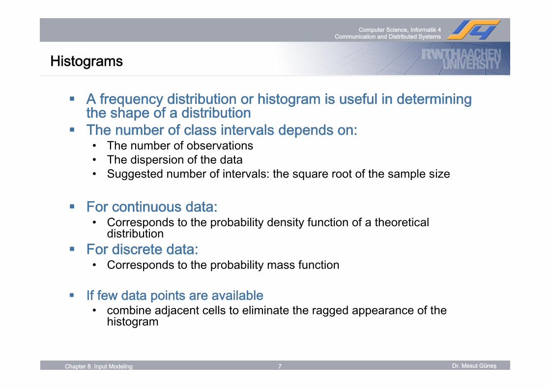
Histograms
A frequency distribution or histogram is useful in determining the shape of a distributionThe number of class intervals depends on:• The number of observations• The dispersion of the data• Suggested number of intervals: the square root of the sample size
For continuous data: • Corresponds to the probability density function of a theoretical
distributionFor discrete data: • Corresponds to the probability mass function
If few data points are available• combine adjacent cells to eliminate the ragged appearance of the
histogram

Dr. Mesut Güneş
Computer Science, Informatik 4 Communication and Distributed Systems
8Chapter 8. Input Modeling
Histograms
Vehicle Arrival Example: Number of vehicles arriving at an intersection between 7 am and 7:05 am was monitored for 100 random workdays.
There are ample data, so the histogram may have a cell for each possible value in the data range
Arrivals per Period Frequency
0 121 102 193 174 105 86 77 58 59 310 311 1
Same data with different interval sizes

Dr. Mesut Güneş
Computer Science, Informatik 4 Communication and Distributed Systems
9Chapter 8. Input Modeling
Histograms – Example
Life tests were performed on electronic components at 1.5 times the nominal voltage, and their lifetime was recorded
1144 ≤ x < 147
…
142 ≤ x < 45
…
112 ≤ x < 15
19 ≤ x < 12
56 ≤ x < 9
103 ≤ x < 6
230 ≤ x < 3
FrequencyComponent Life

Dr. Mesut Güneş
Computer Science, Informatik 4 Communication and Distributed Systems
10Chapter 8. Input Modeling
Histograms – Example
• Target community: cellular network research community
• Traces contain mobility as well as connection information
Available traces• SULAWESI (S.U. Local Area Wireless
Environment Signaling Information)• BALI (Bay Area Location Information)
BALI Characteristics• San Francisco Bay Area• Trace length: 24 hour• Number of cells: 90• Persons per cell: 1100 • Persons at all: 99.000• Active persons: 66.550• Move events: 243.951• Call events: 1.570.807
Question: How to transform the BALI information so that it is usable with a network simulator, e.g., ns-2?
• Node number as well as connection number is too high for ns-2
Stanford University Mobile Activity Traces (SUMATRA)

Dr. Mesut Güneş
Computer Science, Informatik 4 Communication and Distributed Systems
11Chapter 8. Input Modeling
Histograms – Example
Analysis of the BALI Trace• Goal: Reduce the amount of
data by identifying user groupsUser group• Between 2 local minima• Communication characteristic
is kept in the group• A user represents a group
Groups with different mobility characteristics• Intra- and inter group
communicationInteresting characteristic• Number of people with odd
number movements is negligible!
05
1015
200
10
2030
40500
200
400
600
800
1000
1200
1400
1600
1800
Peo
ple
Calls
Movements
-1 0 1 2 3 4 5 6 7 8 9 10 11 12 13 14 15 16 17 18 19
0
5000
10000
15000
20000
25000
Num
ber o
f Peo
ple
Number of Movements

Dr. Mesut Güneş
Computer Science, Informatik 4 Communication and Distributed Systems
12Chapter 8. Input Modeling
Scatter Diagrams
A scatter diagram is a quality tool that can show the relationship between paired data• Random Variable X = Data 1 • Random Variable Y = Data 2 • Draw random variable X on the x-axis and Y on the y-axis
Strong Correlation Moderate Correlation No Correlation

Dr. Mesut Güneş
Computer Science, Informatik 4 Communication and Distributed Systems
13Chapter 8. Input Modeling
Scatter Diagrams
Linear relationship• Correlation: Measures how well data line up• Slope: Measures the steepness of the data• Direction• Y Intercept

Dr. Mesut Güneş
Computer Science, Informatik 4 Communication and Distributed Systems
14Chapter 8. Input Modeling
Selecting the Family of Distributions
A family of distributions is selected based on:• The context of the input variable• Shape of the histogram
Frequently encountered distributions:• Easier to analyze: Exponential, Normal and Poisson
• Harder to analyze: Beta, Gamma and Weibull

Dr. Mesut Güneş
Computer Science, Informatik 4 Communication and Distributed Systems
15Chapter 8. Input Modeling
Selecting the Family of Distributions
Use the physical basis of the distribution as a guide, for example:• Binomial: Number of successes in n trials• Poisson: Number of independent events that occur in a fixed amount of
time or space• Normal: Distribution of a process that is the sum of a number of
component processes• Exponential: time between independent events, or a process time that is
memoryless• Weibull: time to failure for components• Discrete or continuous uniform: models complete uncertainty• Triangular: a process for which only the minimum, most likely, and
maximum values are known• Empirical: resamples from the actual data collected

Dr. Mesut Güneş
Computer Science, Informatik 4 Communication and Distributed Systems
16Chapter 8. Input Modeling
Selecting the Family of Distributions
Remember the physical characteristics of the process• Is the process naturally discrete or continuous valued?• Is it bounded?
No “true” distribution for any stochastic input processGoal: obtain a good approximation

Dr. Mesut Güneş
Computer Science, Informatik 4 Communication and Distributed Systems
17Chapter 8. Input Modeling
Quantile-Quantile Plots
Q-Q plot is a useful tool for evaluating distribution fitIf X is a random variable with CDF F, then the q-quantile of X is the γsuch that
• When F has an inverse, γ = F-1(q)
Let {xi, i = 1,2, …., n} be a sample of data from X and {yj, j = 1,2, …, n} be the observations in ascending order:
• where j is the ranking or order number
, for 0 1F( ) P(X ) q q γ γ= ≤ = < <
1 0.5is approximately -j
j -y F n
⎛ ⎞⎜ ⎟⎝ ⎠
Dr. Mesut Güneş
Computer Science, Informatik 4 Communication and Distributed Systems
18Chapter 8. Input Modeling
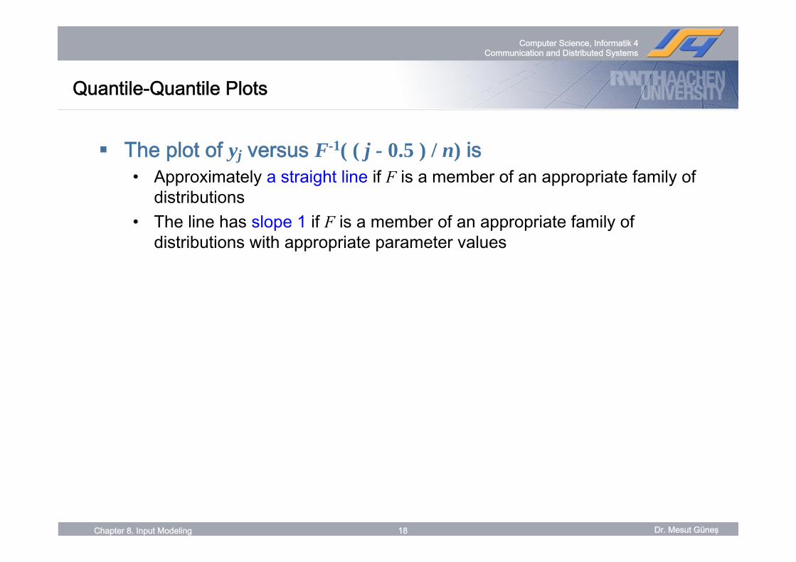
Quantile-Quantile Plots
The plot of yj versus F-1( ( j - 0.5 ) / n) is • Approximately a straight line if F is a member of an appropriate family of
distributions• The line has slope 1 if F is a member of an appropriate family of
distributions with appropriate parameter values

Dr. Mesut Güneş
Computer Science, Informatik 4 Communication and Distributed Systems
19Chapter 8. Input Modeling
Quantile-Quantile Plots
Example: Door installation times of a robot follows a normal distribution.• The observations are ordered from the smallest to the largest:
• yj are plotted versus F-1( (j-0.5)/n) where F has a normal distribution with the sample mean (99.99 sec) and sample variance (0.28322 sec2)
j Value j Value j Value1 99.55 6 99.98 11 100.262 99.56 7 100.02 12 100.273 99.62 8 100.06 13 100.334 99.65 9 100.17 14 100.415 99.79 10 100.23 15 100.47

Dr. Mesut Güneş
Computer Science, Informatik 4 Communication and Distributed Systems
20Chapter 8. Input Modeling
0
0,05
0,1
0,15
0,2
0,25
0,3
0,35
99,4 99,6 99,8 100 100,2 100,4 100,6
Quantile-Quantile Plots
Example (continued): Check whether the door installation times follow a normal distribution.
Superimposed density function of
the normal distribution
99,2
99,4
99,6
99,8
100
100,2
100,4
100,6
100,8
99,2 99,4 99,6 99,8 100 100,2 100,4 100,6 100,8
Straight line, supporting the hypothesis of a
normal distribution

Dr. Mesut Güneş
Computer Science, Informatik 4 Communication and Distributed Systems
21Chapter 8. Input Modeling
Quantile-Quantile Plots
Consider the following while evaluating the linearity of a Q-Q plot:• The observed values never fall exactly on a straight line• The ordered values are ranked and hence not independent, unlikely for
the points to be scattered about the line• Variance of the extremes is higher than the middle. Linearity of the
points in the middle of the plot is more important.
Q-Q plot can also be used to check homogeneity • It can be used to check whether a single distribution can represent two
sample sets• Given two random variables
- X and x1, x2, …, xn- Z and z1, z2, …, zn
• Plotting the ordered values of X and Z against each other reveals approximately a straight line if X and Z are well represented by the same distribution

Dr. Mesut Güneş
Computer Science, Informatik 4 Communication and Distributed Systems
22Chapter 8. Input Modeling
Parameter Estimation
Parameter Estimation: Next step after selecting a family of distributionsIf observations in a sample of size n are X1, X2, …, Xn (discrete or continuous), the sample mean and variance are:
If the data are discrete and have been grouped in a frequency distribution:
• where fj is the observed frequency of value Xj
1 1
2221
−
−== ∑∑ ==
nXnX
Sn
XX
n
i in
i i
1 1
2221
−
−==
∑∑ ==
n
XnXfS
n
XfX
n
j jjn
j jj

Dr. Mesut Güneş
Computer Science, Informatik 4 Communication and Distributed Systems
23Chapter 8. Input Modeling
Parameter Estimation
When raw data are unavailable (data are grouped into class intervals), the approximate sample mean and variance are:
• fj is the observed frequency in the j-th class interval• mj is the midpoint of the j-th interval• c is the number of class intervals
A parameter is an unknown constant, but an estimator is a statistic.
1 1
2221
−
−==
∑∑ ==
n
XnmfS
n
mfX
n
j jjc
j jj

Dr. Mesut Güneş
Computer Science, Informatik 4 Communication and Distributed Systems
24Chapter 8. Input Modeling
Vehicle Arrival Example (continued): Table in the histogram of the example on Slide 8 can be analyzed to obtain:
• The sample mean and variance are
• The histogram suggests X to have a Possion distribution- However, note that sample mean is not equal to sample variance.
– Theoretically: Poisson with parameter λ μ = σ2 = λ- Reason: each estimator is a random variable, it is not perfect.
Parameter Estimation
∑∑ =========
k
j jjk
j jj XfXfXfXfn1
212211 2080 and ,364 and ,...1,10,0,12,100
63.799
)64.3(1002080
3.64100364
22
=
⋅−=
==
S
X
0
5
10
15
20
25
0 1 2 3 4 5 6 7 8 9 10 11Number of Arrivals per Period
Freq
uenc
y

Dr. Mesut Güneş
Computer Science, Informatik 4 Communication and Distributed Systems
25Chapter 8. Input Modeling
Parameter Estimation
Suggested Estimators for Distributions often used in Simulation• Maximum-Likelihood Esitmators
μ, σ2Lognormal
μ, σ2Normal
β, θGamma
λExponential
αPoissonEstimatorParameterDistribution
X=α
X1ˆ =λ
X1ˆ,ˆ =θβ
22ˆ,ˆ SX == σμ22ˆ,ˆ SX == σμ
After taking lnof data.

Dr. Mesut Güneş
Computer Science, Informatik 4 Communication and Distributed Systems
26Chapter 8. Input Modeling
Goodness-of-Fit Tests
Conduct hypothesis testing on input data distribution using• Kolmogorov-Smirnov test • Chi-square test
No single correct distribution in a real application exists • If very little data are available, it is unlikely to reject any candidate
distributions• If a lot of data are available, it is likely to reject all candidate distributions
Be aware of mistakes in decision finding• Type I Error: α• Type II Error: β
State of the null hypothesisStatistical Decision
Type II ErrorCorrectAccept H0
CorrectType I ErrorReject H0
H0 FalseH0 True

Dr. Mesut Güneş
Computer Science, Informatik 4 Communication and Distributed Systems
27Chapter 8. Input Modeling
Chi-Square Test
Intuition: comparing the histogram of the data to the shape of the candidate density or mass functionValid for large sample sizes when parameters are estimated by maximum-likelihoodArrange the n observations into a set of k class intervalsThe test statistic is:
• approximately follows the chi-square distribution with k-s-1degrees of freedom
• s = number of parameters of the hypothesized distribution estimated by the sample statistics.
∑=
−=
k
i i
ii
EEO
1
220
)(χ
Observed Frequency in the i-th class
Expected FrequencyEi = n*pi
where pi is the theoretical prob. of the i-th interval.Suggested Minimum = 5
20χ

Dr. Mesut Güneş
Computer Science, Informatik 4 Communication and Distributed Systems
28Chapter 8. Input Modeling
Chi-Square Test
The hypothesis of a chi-square test isH0: The random variable, X, conforms to the distributional assumption with the parameter(s) given by the estimate(s).H1: The random variable X does not conform.
H0 is rejected if
If the distribution tested is discrete and combining adjacent cell is not required (so that Ei > minimum requirement):• Each value of the random variable should be a class interval, unless
combining is necessary, and
) x P(X ) p(x p iii ===
21,
20 −−> skαχχ

Dr. Mesut Güneş
Computer Science, Informatik 4 Communication and Distributed Systems
29Chapter 8. Input Modeling
Chi-Square Test
If the distribution tested is continuous:
• where ai-1 and ai are the endpoints of the i-th class interval• f(x) is the assumed pdf, F(x) is the assumed cdf• Recommended number of class intervals (k):
• Caution: Different grouping of data (i.e., k) can affect the hypothesis testing result.
)()( )( 11
−−== ∫−
ii
a
ai aFaFdxxf p i
i
Sample Size, n Number of Class Intervals, k
20 Do not use the chi-square test
50 5 to 10
100 10 to 20
> 100 n1/2 to n/5

Dr. Mesut Güneş
Computer Science, Informatik 4 Communication and Distributed Systems
30Chapter 8. Input Modeling
Chi-Square Test
Vehicle Arrival Example (continued): H0: the random variable is Poisson distributed.H1: the random variable is not Poisson distributed.
• Degree of freedom is k-s-1 = 7-1-1 = 5, hence, the hypothesis is rejected at the 0.05 level of significance.
!
)(
xen
xnpEx
i
αα−
=
=xi Observed Frequency, Oi Expected Frequency, Ei (Oi - Ei)2/Ei
0 12 2.61 10 9.62 19 17.4 0.153 17 21.1 0.84 19 19.2 4.415 6 14.0 2.576 7 8.5 0.267 5 4.48 5 2.09 3 0.8
10 3 0.3> 11 1 0.1
100 100.0 27.68
7.87
11.62
Combined because of the assumption of
min Ei = 5, e.g.,
E1 = 2.6 < 5, hence combine with E2
1.1168.27 25,05.0
20 =>= χχ
22
17
12.2
7.6

Dr. Mesut Güneş
Computer Science, Informatik 4 Communication and Distributed Systems
31Chapter 8. Input Modeling
Kolmogorov-Smirnov Test
Intuition: formalize the idea behind examining a Q-Q plotRecall • The test compares the continuous cdf, F(x), of the hypothesized
distribution with the empirical cdf, SN(x), of the N sample observations. • Based on the maximum difference statistics
D = max| F(x) - SN(x) |
A more powerful test, particularly useful when:• Sample sizes are small• No parameters have been estimated from the data
When parameter estimates have been made:• Critical values are biased, too large.• More conservative, i.e., smaller Type I error than specified.

Dr. Mesut Güneş
Computer Science, Informatik 4 Communication and Distributed Systems
32Chapter 8. Input Modeling
p-Values and “Best Fits”
p-value for the test statistics• The significance level at which one would just reject H0 for the given test
statistic value.• A measure of fit, the larger the better• Large p-value: good fit• Small p-value: poor fit
Vehicle Arrival Example (cont.): • H0: data is Poisson• Test statistics: , with 5 degrees of freedom• p-value = 0.00004, meaning we would reject H0 with 0.00004 significance
level, hence Poisson is a poor fit.
68.2720 =χ

Dr. Mesut Güneş
Computer Science, Informatik 4 Communication and Distributed Systems
33Chapter 8. Input Modeling
p-Values and “Best Fits”
Many software use p-value as the ranking measure to automatically determine the “best fit”. Things to be cautious about:• Software may not know about the physical basis of the data, distribution
families it suggests may be inappropriate.• Close conformance to the data does not always lead to the most
appropriate input model.• p-value does not say much about where the lack of fit occurs
Recommended: always inspect the automatic selection using graphical methods.

Dr. Mesut Güneş
Computer Science, Informatik 4 Communication and Distributed Systems
34Chapter 8. Input Modeling
Fitting a Non-stationary Poisson Process
Fitting a NSPP to arrival data is difficult, possible approaches:• Fit a very flexible model with lots of parameters• Approximate constant arrival rate over some basic interval of
time, but vary it from time interval to time interval.Suppose we need to model arrivals over time [0,T], our approach is the most appropriate when we can:• Observe the time period repeatedly• Count arrivals / record arrival times• Divide the time period into k equal intervals of length Δt =T/k• Over n periods of observation let Cij be the number of arrivals
during the i-th interval on the j-th period

Dr. Mesut Güneş
Computer Science, Informatik 4 Communication and Distributed Systems
35Chapter 8. Input Modeling
Fitting a Non-stationary Poisson Process
The estimated arrival rate during the i-th time period (i-1) Δt < t ≤ i Δt is:
• n = Number of observation periods, • Δt = time interval length• Cij = # of arrivals during the i-th time interval on the j-th observation
periodExample: Divide a 10-hour business day [8am,6pm] into equal intervals k = 20 whose length Δt = ½, and observe over n=3 days
∑=Δ
=n
jijC
tnt
1
1)(λ
Day 1 Day 2 Day 3
8:00 - 8:30 12 14 10 24
8:30 - 9:00 23 26 32 54
9:00 - 9:30 27 18 32 52
9:30 - 10:00 20 13 12 30
Number of ArrivalsTime Period
Estimated Arrival Rate (arrivals/hr) For instance,
1/3(0.5)*(23+26+32)= 54 arrivals/hour

Dr. Mesut Güneş
Computer Science, Informatik 4 Communication and Distributed Systems
36Chapter 8. Input Modeling
Selecting Model without Data
If data is not available, some possible sources to obtain information about the process are:• Engineering data: often product or process has performance
ratings provided by the manufacturer or company rules specify time or production standards.
• Expert option: people who are experienced with the process or similar processes, often, they can provide optimistic, pessimistic and most-likely times, and they may know the variability as well.
• Physical or conventional limitations: physical limits on performance, limits or bounds that narrow the range of the inputprocess.
• The nature of the process.The uniform, triangular, and beta distributions are often used as input models.• Speed of a vehicle?

Dr. Mesut Güneş
Computer Science, Informatik 4 Communication and Distributed Systems
37Chapter 8. Input Modeling
Selecting Model without Data
Example: Production planning simulation.
• Input of sales volume of various products is required, salesperson of product XYZ says that:
- No fewer than 1000 units and no more than 5000 units will be sold.
- Given her experience, she believes there is a 90% chance of selling more than 2000 units, a 25% chance of selling more than 2500 units, and only a 1% chance of selling more than 4500 units.
• Translating these information into a cumulative probability of being less than or equal to those goals for simulation input:
1,000,014500 < X <= 50004
0,990,242500 < X <= 45003
0,750,652000 < X <=25002
0,100,11000 <= X <= 20001
CumulativeFrequency, ciInterval (Sales)i
0,00
0,20
0,40
0,60
0,80
1,00
1,20
1000 <= X <= 2000 2000 < X <=2500 2500 < X <= 4500 4500 < X <= 5000

Dr. Mesut Güneş
Computer Science, Informatik 4 Communication and Distributed Systems
38Chapter 8. Input Modeling
Multivariate and Time-Series Input Models
The random variable discussed until now were considered to be independent of any other variables within the context of the problem• However, variables may be related• If they appear as input, the relationship should be investigated and taken
into considerationMultivariate input models• Fixed, finite number of random variables• For example, lead time and annual demand for an inventory model• An increase in demand results in lead time increase, hence variables are
dependent.Time-series input models• Infinite sequence of random variables• For example, time between arrivals of orders to buy and sell stocks• Buy and sell orders tend to arrive in bursts, hence, times between arrivals
are dependent.

Dr. Mesut Güneş
Computer Science, Informatik 4 Communication and Distributed Systems
39Chapter 8. Input Modeling
Covariance and Correlation
Consider the model that describes relationship between X1 and X2:
• β = 0, X1 and X2 are statistically independent• β > 0, X1 and X2 tend to be above or below their means together• β < 0, X1 and X2 tend to be on opposite sides of their means
Covariance between X1 and X2:
Covariance between X1 and X2:
• where
εμβμ +−=− )()( 2211 XX
2121221121 )()])([(),cov( μμμμ −=−−= XXEXXEXX
ε is a random variable with mean 0 and is independent
of X2
⎪⎩
⎪⎨
⎧
><=
⎪⎩
⎪⎨
⎧⇒
><=
000
000
),cov( 21 βXX ∞<<∞ ),cov( 21 XX

Dr. Mesut Güneş
Computer Science, Informatik 4 Communication and Distributed Systems
40Chapter 8. Input Modeling
Covariance and Correlation
Correlation between X1 and X2 (values between -1 and 1):
• where
• The closer ρ is to -1 or 1, the stronger the linear relationship is betweenX1 and X2.
21
2121
),cov(),(corrσσ
ρ XXXX ==
⎪⎩
⎪⎨
⎧
><=
⇒⎪⎩
⎪⎨
⎧
><=
000
000
),( 21 βXXcorr

Dr. Mesut Güneş
Computer Science, Informatik 4 Communication and Distributed Systems
41Chapter 8. Input Modeling
Covariance and Correlation
A time series is a sequence of random variables X1, X2, X3,…which are identically distributed (same mean and variance) but dependent.• cov(Xt, Xt+h) is the lag-h autocovariance• corr(Xt, Xt+h) is the lag-h autocorrelation• If the autocovariance value depends only on h and not on t, the
time series is covariance stationary• For covariance stationary time series, the shorthand for lag-h is
used
Notice• autocorrelation measures the dependence between random
variables that are separated by h-1
),( htth XXcorr +=ρ

Dr. Mesut Güneş
Computer Science, Informatik 4 Communication and Distributed Systems
42Chapter 8. Input Modeling
Multivariate Input Models
If X1 and X2 are normally distributed, dependence between them can be modeled by the bivariate normal distribution with μ1, μ2, σ1
2, σ22
and correlation ρ• To estimate μ1, μ2, σ1
2, σ22, see “Parameter Estimation”
• To estimate ρ, suppose we have n independent and identically distributed pairs (X11, X21), (X12, X22), … (X1n, X2n),
• Then the sample covariance is
• The sample correlation is
∑=
−−−
=n
jjj XXXX
nXX
1221121 ))((
11),v(oc
21
21
ˆˆ),v(ocˆ
σσρ XX
=Sample deviation

Dr. Mesut Güneş
Computer Science, Informatik 4 Communication and Distributed Systems
43Chapter 8. Input Modeling
Multivariate Input Models - Example
Let X1 the average lead time to deliver and X2 the annual demandfor a product.Data for 10 years is available.
Lead time and demand are strongly dependent.• Before accepting this model, lead time and demand should be checked
individually to see whether they are represented well by normal distribution.
966,3
924,5
1097,3
1065,8
1046,9
1126,9
976,0
1166,9
834,3
1036,5
Demand(X2)
Lead Time (X1)
93.9,8.10102.1,14.6
22
11
==
==
σσ
XX
66.8sample =c
86.093.902.1
66.8ˆ =⋅
=ρ
Covariance

Dr. Mesut Güneş
Computer Science, Informatik 4 Communication and Distributed Systems
44Chapter 8. Input Modeling
Time-Series Input Models
If X1, X2, X3,… is a sequence of identically distributed, but dependentand covariance-stationary random variables, then we can represent the process as follows:• Autoregressive order-1 model, AR(1)• Exponential autoregressive order-1 model, EAR(1)
- Both have the characteristics that:
- Lag-h autocorrelation decreases geometrically as the lag increases, hence, observations far apart in time are nearly independent
,...2,1for ,),( === + hXXcorr hhtth ρρ

Dr. Mesut Güneş
Computer Science, Informatik 4 Communication and Distributed Systems
45Chapter 8. Input Modeling
AR(1) Time-Series Input Models
Consider the time-series model:
If initial value X1 is chosen appropriately, then • X1, X2, … are normally distributed with mean = μ, and variance = σ2/(1-φ2)• Autocorrelation ρh = φh
To estimate φ, μ, σε2 :
,...3,2for ,)( 1 =+−+= − tXX ttt εμφμ2
32 varianceand 0 with ddistributenormally i.i.d. are , , where εε σμεε =…
21
ˆ),v(ocˆ
σφ += tt XX
anceautocovari 1 theis ),v(oc where 1 lag-XX tt +
, ˆ X=μ , )ˆ1(ˆˆ 222 φσσε −=
Dr. Mesut Güneş
Computer Science, Informatik 4 Communication and Distributed Systems
46Chapter 8. Input Modeling
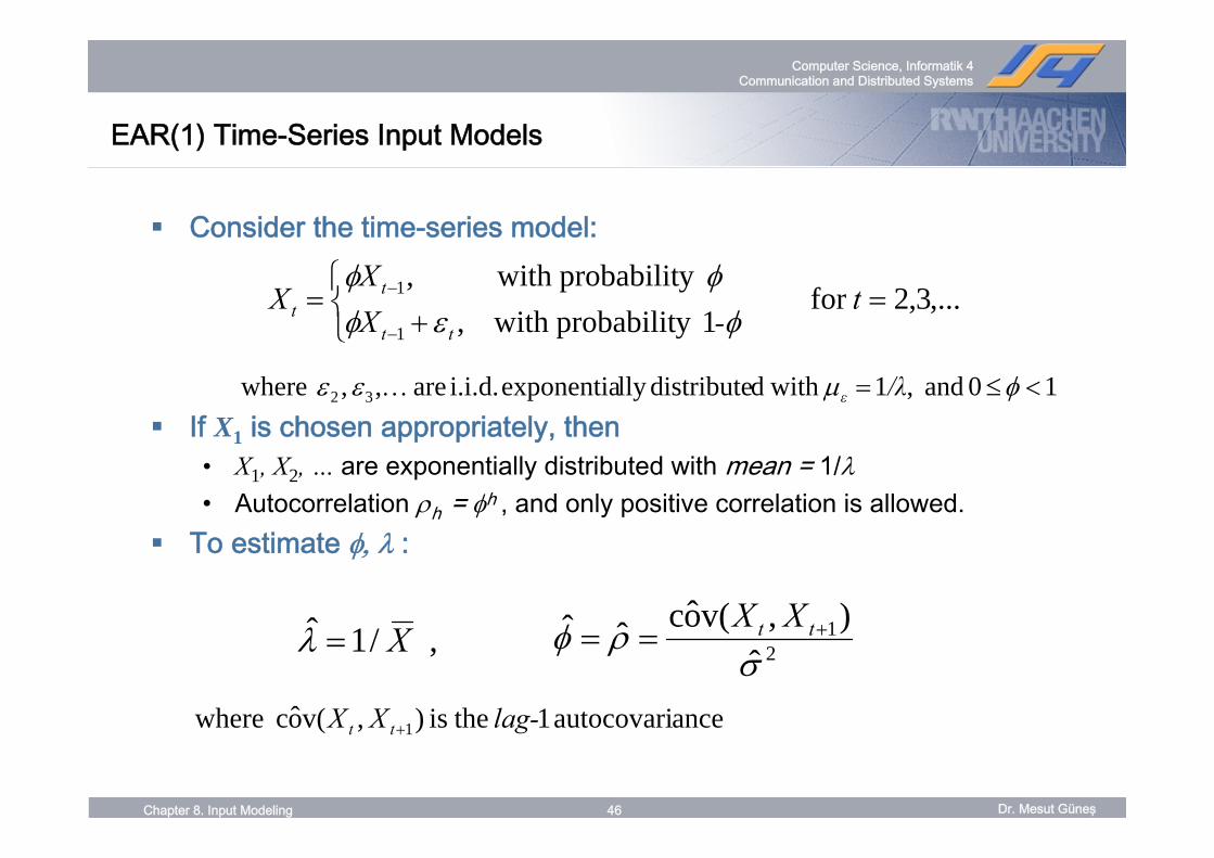
EAR(1) Time-Series Input Models
Consider the time-series model:
If X1 is chosen appropriately, then • X1, X2, … are exponentially distributed with mean = 1/λ• Autocorrelation ρh = φh , and only positive correlation is allowed.
To estimate φ, λ :
,...3,2for 1y probabilit with ,
y probabilit with ,
1
1 =⎩⎨⎧
+=
−
− t-X
XX
tt
tt φεφ
φφ
1 0 and ,1 with ddistributelly exponentia i.i.d. are , , where 32 <≤=… φμεε /λε
21
ˆ),v(ocˆˆ
σρφ +== tt XX
anceautocovari 1 theis ),v(oc where 1 lag-XX tt +
, /1ˆ X=λ

Dr. Mesut Güneş
Computer Science, Informatik 4 Communication and Distributed Systems
47Chapter 8. Input Modeling
Summary
In this chapter, we described the 4 steps in developing input data models:1) Collecting the raw data2) Identifying the underlying statistical distribution3) Estimating the parameters4) Testing for goodness of fit