discrete fourier transform - kasetsart universityjan/dsp/note/lecture-08-2-r05.pdf · discrete...

Digital Signal Processing, © 2011 Robi Polikar, Rowan University

Discrete Fourier Transform

http://engineering.rowan.edu/

http://users.rowan.edu/~polikar/RESEARCH

http://engineering.rowan.edu/~polikar

http://engineering.rowan.edu/~polikar

This Week in DSP

Discrete Fourier Transform Analysis, Synthesis and orthogonality of discrete complex exponentials

Periodicity of DFT

Circular Shift

Properties of DFT

Circular Convolution Linear vs. circular convolution

Computing convolution using DFT

Some examples

The DFT matrix

The relationship between DTFT vs DFT: Reprise

FFT

Analyzing streaming data:

Overlap add & overlap save

RP Robi Polikar – All Rights Reserved © 2004 – 2011.

M Mitra – All Rights Reserved , Wiley © 2011.



DFT

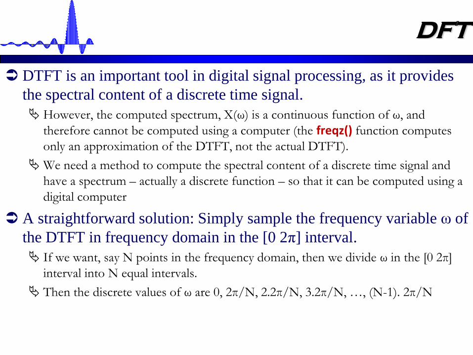
DTFT is an important tool in digital signal processing, as it provides

the spectral content of a discrete time signal.

However, the computed spectrum, X(ω) is a continuous function of ω, and

therefore cannot be computed using a computer (the freqz() function computes

only an approximation of the DTFT, not the actual DTFT).

We need a method to compute the spectral content of a discrete time signal and

have a spectrum – actually a discrete function – so that it can be computed using a

digital computer

A straightforward solution: Simply sample the frequency variable ω of

the DTFT in frequency domain in the [0 2π] interval.

If we want, say N points in the frequency domain, then we divide ω in the [0 2π]

interval into N equal intervals.

Then the discrete values of ω are 0, 2π/N, 2.2π/N, 3.2π/N, …, (N-1). 2π/N



DFT Analysis

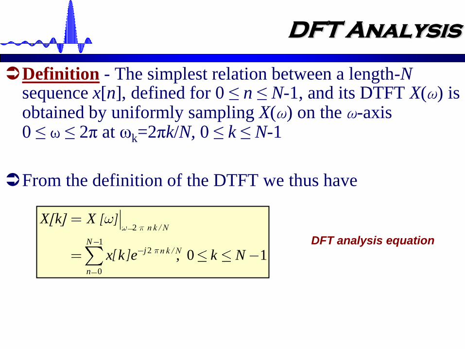
Definition - The simplest relation between a length-Nsequence x[n], defined for 0 ≤ n ≤ N-1, and its DTFT X(ω) is obtained by uniformly sampling X(ω) on the ω-axis 0 ≤ ω ≤ 2π at ωk=2πk/N, 0 ≤ k ≤ N-1

From the definition of the DTFT we thus have

2

12

0

, 0 1

n k / NN

j

n

X[k] X

x k e k NDFT analysis equation

[ ]

[ ]

n k / N



DFT Analysis

Note the following:

k replaces as the frequency variable in the discrete frequency domain

X[k] is also (usually) a length-N sequence in the frequency domain, just like the

signal x[n] is a length-N sequence in the time domain.

X[k] can be made to be longer than N points ( as we will later see)

The sequence X[k] is called the discrete Fourier transform (DFT) of the

sequence x[n]

Using the notation the DFT is usually expressed as:NjN eW /2

1

0

, 0 1N

k n

N

n

X k x n W k N[ ] [ ]



Inverse DFT

(DFT Synthesis)

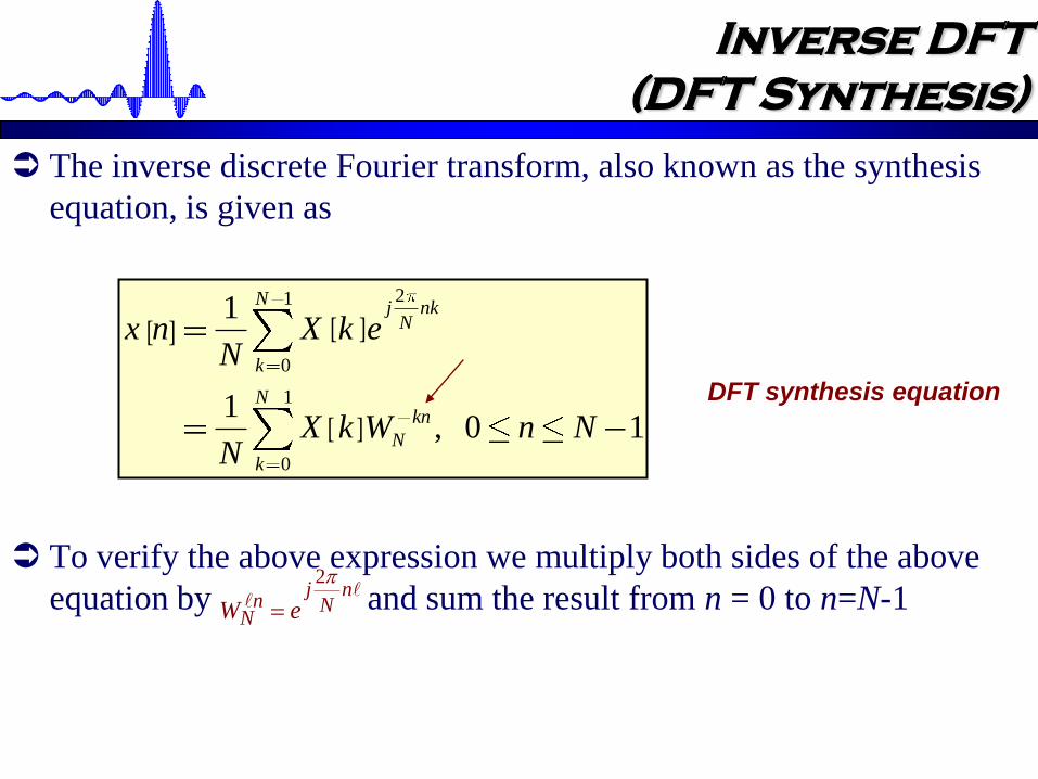
The inverse discrete Fourier transform, also known as the synthesis

equation, is given as

To verify the above expression we multiply both sides of the above

equation by and sum the result from n = 0 to n=N-1

21

0

1

0

1

1, 0 1

Nj nk

N

k

Nkn

N

k

x n X k eN

X k W n NN

DFT synthesis equation

nN

jn

N eW

2

[ ] [ ]

[ ]



Orthogonality of

Discrete Exponentials

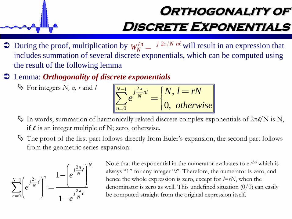
During the proof, multiplication by will result in an expression that

includes summation of several discrete exponentials, which can be computed using

the result of the following lemma

Lemma: Orthogonality of discrete exponentials

For integers N, n, r and l

In words, summation of harmonically related discrete complex exponentials of 2πl/N is N,

if l is an integer multiple of N; zero, otherwise.

The proof of the first part follows directly from Euler’s expansion, the second part follows

from the geometric series expansion:

2j N nnNW

21

0

,

0,

Nj nl

N

n

N l rNe

otherwise

2

21

20

1

1

Nj

Nn

Nj

N

jn N

e

e

e

Note that the exponential in the numerator evaluates to e j2πl which is

always “1” for any integer “l”. Therefore, the numerator is zero, and

hence the whole expression is zero, except for l=rN, when the

denominator is zero as well. This undefined situation (0/0) can easily

be computed straight from the original expression itself.




Computing DFT

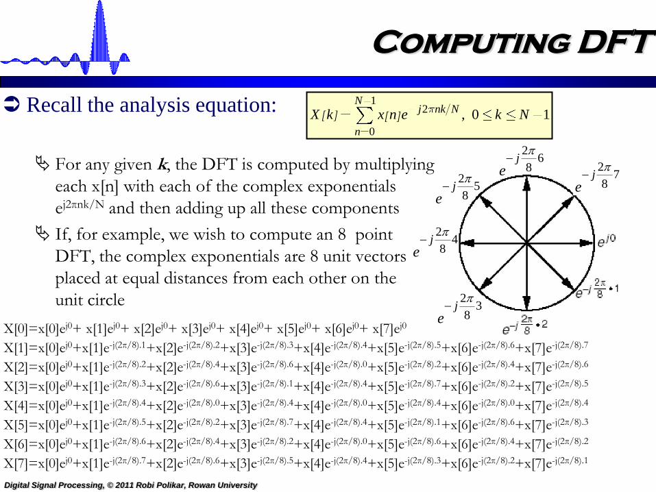
Recall the analysis equation:

For any given k, the DFT is computed by multiplying

each x[n] with each of the complex exponentials

ej2πnk/N and then adding up all these components

If, for example, we wish to compute an 8 point

DFT, the complex exponentials are 8 unit vectors

placed at equal distances from each other on the

unit circle

12

0

, 0 1N

j nk N

n

X k x n e k N

X[0]=x[0]ej0+ x[1]ej0+ x[2]ej0+ x[3]ej0+ x[4]ej0+ x[5]ej0+ x[6]ej0+ x[7]ej0

X[1]=x[0]ej0+x[1]e-j(2π/8).1+x[2]e-j(2π/8).2+x[3]e-j(2π/8).3+x[4]e-j(2π/8).4+x[5]e-j(2π/8).5+x[6]e-j(2π/8).6+x[7]e-j(2π/8).7







38

2j

e

48

2j

e

58

2j

e

68

2j

e

78

2j

e

[ ] [ ]



Periodicity in DFT

DFT is periodic in both time and frequency domains!!!

Even though the original time domain sequence to be transformed is not periodic!

There are several ways to explain this phenomenon. Mathematically ,

we can easily show that both the analysis and synthesis equations are

periodic by N.

Now, understanding that DFT is periodic in frequency domain is

straightforward: DFT is obtained by sampling DTFT at 2π/N intervals.

Since DTFT was periodic with 2π DFT is periodic by N.

This can also be seen easily from the complex exponential wheel.

Since there are only N vectors around a unit circle, the transform will

repeat itself every N points.

But what does it mean that DFT is also periodic in

time domain?



Periodicity in DFT

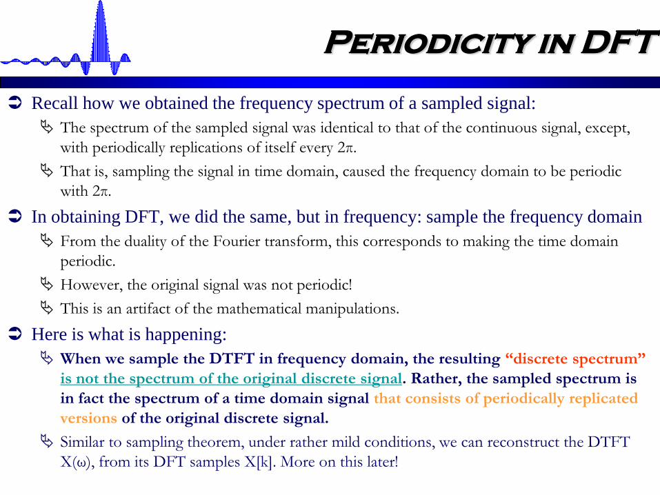
Recall how we obtained the frequency spectrum of a sampled signal:

The spectrum of the sampled signal was identical to that of the continuous signal, except,

with periodically replications of itself every 2π.

That is, sampling the signal in time domain, caused the frequency domain to be periodic

with 2π.

In obtaining DFT, we did the same, but in frequency: sample the frequency domain

From the duality of the Fourier transform, this corresponds to making the time domain

periodic.

However, the original signal was not periodic!

This is an artifact of the mathematical manipulations.

Here is what is happening:

When we sample the DTFT in frequency domain, the resulting “discrete spectrum”

is not the spectrum of the original discrete signal. Rather, the sampled spectrum is

in fact the spectrum of a time domain signal that consists of periodically replicated

versions of the original discrete signal.

Similar to sampling theorem, under rather mild conditions, we can reconstruct the DTFT

X(ω), from its DFT samples X[k]. More on this later!



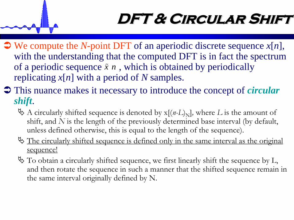
DFT & Circular Shift

We compute the N-point DFT of an aperiodic discrete sequence x[n], with the understanding that the computed DFT is in fact the spectrum of a periodic sequence , which is obtained by periodically replicating x[n] with a period of N samples.

This nuance makes it necessary to introduce the concept of circular shift. A circularly shifted sequence is denoted by x[(n-L)N], where L is the amount of

shift, and N is the length of the previously determined base interval (by default, unless defined otherwise, this is equal to the length of the sequence).

The circularly shifted sequence is defined only in the same interval as the original sequence!

To obtain a circularly shifted sequence, we first linearly shift the sequence by L, and then rotate the sequence in such a manner that the shifted sequence remain in the same interval originally defined by N.

x n



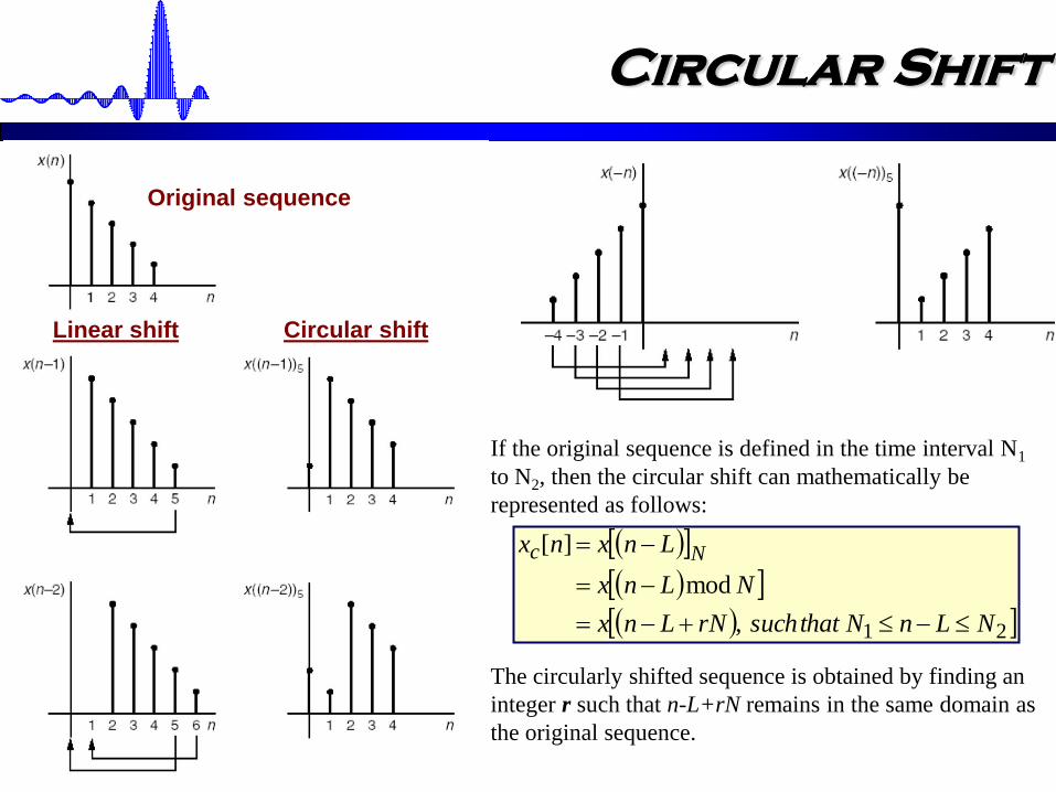
Circular Shift

Original sequence

Linear shift Circular shift

If the original sequence is defined in the time interval N1

to N2, then the circular shift can mathematically be

represented as follows:

21,

mod

][

NLnNthatsuchrNLnx

NLnx

Lnxnx Nc

The circularly shifted sequence is obtained by finding an

integer r such that n-L+rN remains in the same domain as

the original sequence.



Properties of the DFT

(Circular convolution in frequency)

][0

2

kGekn

Nj

][0

2

ngenk

Nj

Nnhng ][*][

NkHkGN

][*][1



DFT Symmetry relations

M



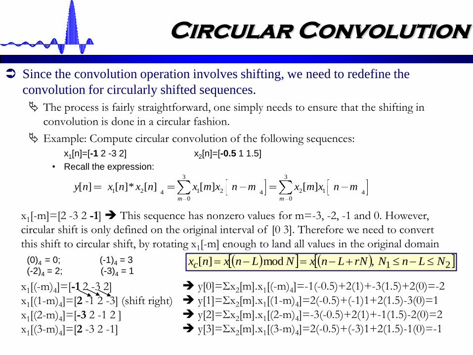
Circular Convolution

Since the convolution operation involves shifting, we need to redefine the

convolution for circularly shifted sequences.

The process is fairly straightforward, one simply needs to ensure that the shifting in

convolution is done in a circular fashion.

Example: Compute circular convolution of the following sequences:

x1[n]=[-1 2 -3 2] x2[n]=[-0.5 1 1.5]

• Recall the expression:3 3

1 2 1 2 2 14 4 40 0

[ ] [ ]* [ ] [ ] [ ]m m

y n x n x n x m x n m x m x n m

x1[-m]=[2 -3 2 -1] This sequence has nonzero values for m=-3, -2, -1 and 0. However,

circular shift is only defined on the original interval of [0 3]. Therefore we need to convert

this shift to circular shift, by rotating x1[-m] enough to land all values in the original domain

x1[(-m)4]=[-1 2 -3 2]

x1[(1-m)4]=[2 -1 2 -3] (shift right)

x1[(2-m)4]=[-3 2 -1 2 ]

x1[(3-m)4]=[2 -3 2 -1]

21,mod][ NLnNrNLnxNLnxnxc

y[0]=Σx2[m].x1[(-m)4]=-1(-0.5)+2(1)+-3(1.5)+2(0)=-2

y[1]=Σx2[m].x1[(1-m)4]=2(-0.5)+(-1)1+2(1.5)-3(0)=1

y[2]=Σx2[m].x1[(2-m)4]=-3(-0.5)+2(1)+-1(1.5)-2(0)=2

y[3]=Σx2[m].x1[(3-m)4]=2(-0.5)+(-3)1+2(1.5)-1(0)=-1

(0)4 = 0; (-1)4 = 3

(-2)4 = 2; (-3)4 = 1



Circular Convolution

Example

Compute circular convolution of x[n]=[1 3 2 -1 4], h[n]=[2 0 1 7 -3]

4 4

5 5 50 0

[ ] [ ]* [ ] [ ] [ ]m m

y n x n h n x m h n m h m x n m

x[m]=[1 3 2 -1 4]

h[-m]=[-3 7 1 0 2]

h[(-m)5]=[2 -3 7 1 0] y[0]=Σx[m].h[(-m)5]=1*2+3(-3)+2*7+-1(1)+4(0)=6

h[(1-m)5]=[0 2 -3 7 1] y[1]=Σx[m].h[(1-m)5]=-3

h[(2-m)5]=[1 0 2 -3 7] y[2]=Σx[m].h[(2-m)5]= 36

h[(3-m)5]=[7 1 0 2 -3] y[3]=Σx[m].h[(3-m)5]= -4

h[(4-m)5]=[-3 7 1 0 2] y[4]=Σx[m].h[(4-m)5]= 28

Linear convolution results: [ 2 6 5 8 28 4 -9 31 -12]



Linear vs. Circular

Convolution

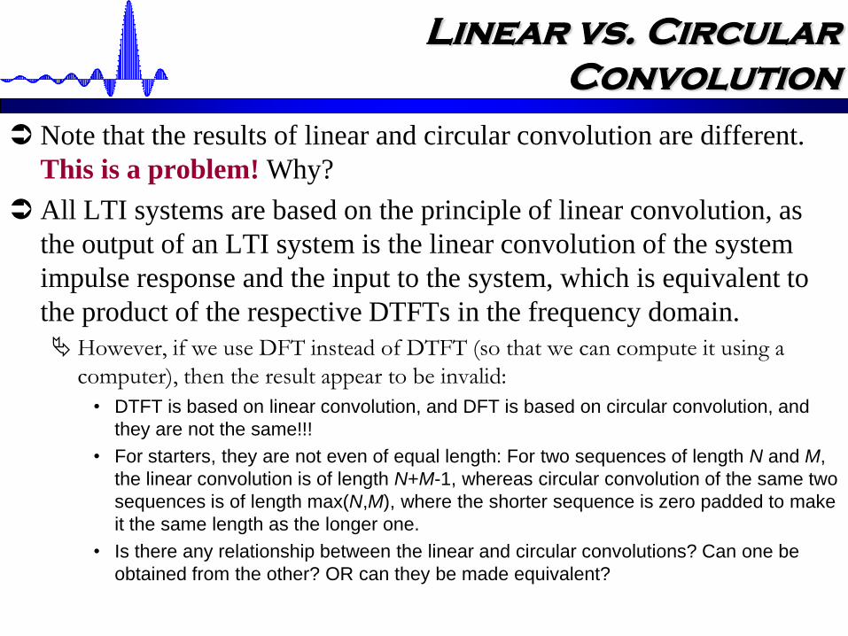
Note that the results of linear and circular convolution are different.

This is a problem! Why?

All LTI systems are based on the principle of linear convolution, as

the output of an LTI system is the linear convolution of the system

impulse response and the input to the system, which is equivalent to

the product of the respective DTFTs in the frequency domain.

However, if we use DFT instead of DTFT (so that we can compute it using a

computer), then the result appear to be invalid:

• DTFT is based on linear convolution, and DFT is based on circular convolution, and

they are not the same!!!

• For starters, they are not even of equal length: For two sequences of length N and M,

the linear convolution is of length N+M-1, whereas circular convolution of the same two

sequences is of length max(N,M), where the shorter sequence is zero padded to make

it the same length as the longer one.

• Is there any relationship between the linear and circular convolutions? Can one be

obtained from the other? OR can they be made equivalent?



Linear vs. Circular

Convolution

YES!, rather easily, as a matter of fact!

FACT: If we zero pad both sequences x[n] and h[n], so that they are both of

length N+M-1, then linear convolution and circular convolution result in identical

sequences

Furthermore: If the respective DFTs of the zero padded sequences are X[k] and

H[k], then the inverse DFT of X[k]∙H[k] is equal to the linear convolution of x[n]

and h[n]

Note that, normally, the inverse DFT of X[k].H[k] is the circular convolution of

x[n] and h[n]. If they are zero padded, then the inverse DFT is also the linear

convolution of the two.



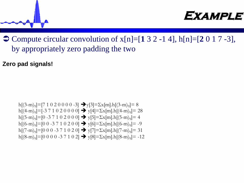
Example

Compute circular convolution of x[n]=[1 3 2 -1 4], h[n]=[2 0 1 7 -3],

by appropriately zero padding the two

We need 5+5-1=9 samples

h[(3-m)9]=[7 1 0 2 0 0 0 0 -3] y[3]=Σx[m].h[(3-m)9]= 8h[(4-m)9]=[-3 7 1 0 2 0 0 0 0] y[4]=Σx[m].h[(4-m)9]= 28

h[(5-m)9]=[0 -3 7 1 0 2 0 0 0] y[5]=Σx[m].h[(5-m)9]= 4

h[(6-m)9]=[0 0 -3 7 1 0 2 0 0] y[6]=Σx[m].h[(6-m)9]= -9

h[(7-m)9]=[0 0 0 -3 7 1 0 2 0] y[7]=Σx[m].h[(7-m)9]= 31

h[(8-m)9]=[0 0 0 0 -3 7 1 0 2] y[8]=Σx[m].h[(8-m)9]= -12

Zero pad signals!



Computing Convolution

Using DFT

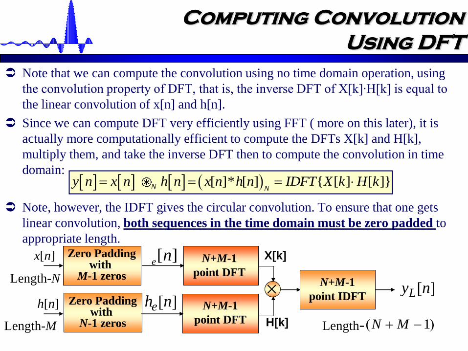
Note that we can compute the convolution using no time domain operation, using

the convolution property of DFT, that is, the inverse DFT of X[k]∙H[k] is equal to

the linear convolution of x[n] and h[n].

Since we can compute DFT very efficiently using FFT ( more on this later), it is

actually more computationally efficient to compute the DFTs X[k] and H[k],

multiply them, and take the inverse DFT then to compute the convolution in time

domain:

Note, however, the IDFT gives the circular convolution. To ensure that one gets

linear convolution, both sequences in the time domain must be zero padded to

appropriate length.

[ ]* [ ] { [ ] [ ]}N Ny n x n h n x n h n IDFT X k H k

Zero Paddingwith

M-1 zeros

N+M-1

point DFT

x[n]

h[n]

Length-N

[ ]e n

][nhe

][nyL

Length-M Length- )( 1 MN

Zero Paddingwith

N-1 zeros

N+M-1

point DFT

X[k]

H[k]

N+M-1

point IDFT



Example

x=[1 3 2 -1 4];

h=[2 0 1 7 -3];

x2=[1 3 2 -1 4 0 0 0 0];

h2=[2 0 1 7 -3 0 0 0 0];

C1=conv(x,h);

X=fft(x2); H=fft(h2);

C2=ifft(X.*H);

subplot(411)

stem(x, 'filled'); grid

subplot(412)

stem(h, 'filled'); grid

subplot(413)

stem(C1, 'filled'); grid

subplot(414)

stem(real(C2), 'filled'); grid

RP



Convolution Matrix

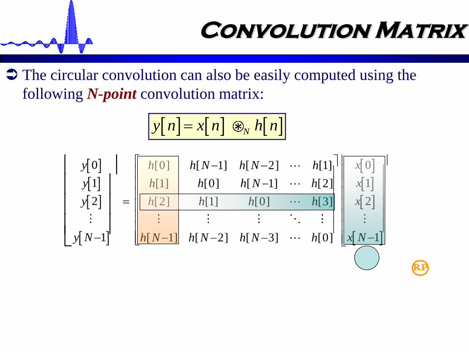
The circular convolution can also be easily computed using the

following N-point convolution matrix:

0 0[0] [ 1] [ 2] [1]

1 1[1] [0] [ 1] [2]

2 2[2] [1] [0] [3]

1 1[ 1] [ 2] [ 3] [0]

y xh h N h N h

y xh h h N h

y xh h h h

y N x Nh N h N h N h

Ny n x n h n

RP



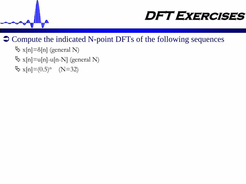
DFT Exercises

Compute the indicated N-point DFTs of the following sequences

x[n]=δ[n] (general N)

x[n]=u[n]-u[n-N] (general N)

x[n]=(0.5)n (N=32)



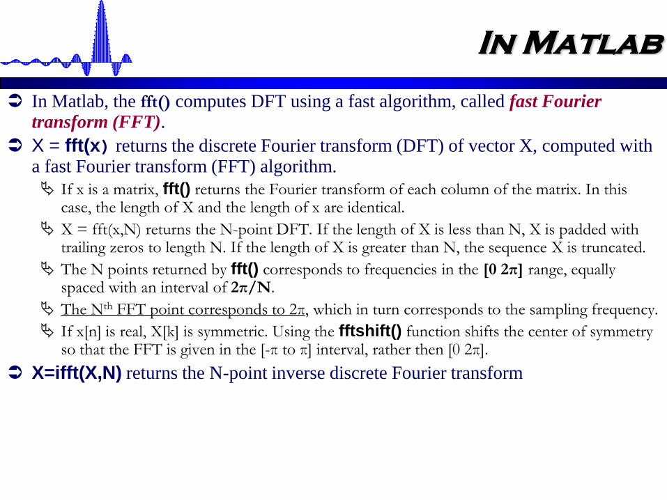
In Matlab

In Matlab, the fft() computes DFT using a fast algorithm, called fast Fourier transform (FFT).

X = fft(x) returns the discrete Fourier transform (DFT) of vector X, computed with a fast Fourier transform (FFT) algorithm.

If x is a matrix, fft() returns the Fourier transform of each column of the matrix. In this case, the length of X and the length of x are identical.

X = fft(x,N) returns the N-point DFT. If the length of X is less than N, X is padded with trailing zeros to length N. If the length of X is greater than N, the sequence X is truncated.

The N points returned by fft() corresponds to frequencies in the [0 2π] range, equally spaced with an interval of 2π/N.

The Nth FFT point corresponds to 2π, which in turn corresponds to the sampling frequency.

If x[n] is real, X[k] is symmetric. Using the fftshift() function shifts the center of symmetry so that the FFT is given in the [-π to π] interval, rather then [0 2π].

X=ifft(X,N) returns the N-point inverse discrete Fourier transform



An Example

312 32

0

312 32

0

312 32

0

322 32

2 32

0.9

0.9

1 0.9

1 0.9

j nk

n

n j nk

n

nj k

n

j k

j k

X k x n e

e

e

e

e

0.9 , 32nx n N

0

0

0

0.9

0.9

1

1 0.9

j n

n

n j n

n

nj

n

j

X x n e

e

e

e

0.9nx n u n

DFTDTFT

X[k]=DFT (x[n])

X[] = DTFT (x[n])

[ ] [ ] ( ) [ ]



Back to Example

n=0:31; k=0:31;

x=0.9.^n;

w=linspace(0, 2*pi, 512); %512 point DTFT

K=linspace(0, 2*pi, 32); %32 point DFT

X1=1./(1-0.9*exp(-j*w)); %DTFT of x[n]

X2=(1-(0.9*exp(-j*(2*pi/32)*k)).^32)./

(1-0.9*exp(-j*(2*pi/32)*k)); %DFT of x[n]

X=fft(x);

subplot(311)

plot(w, abs(X1)); grid

subplot(312)

stem(K, abs(X2), 'r', 'filled'); grid

subplot(313)

stem(K, abs(X), 'g', 'filled'); grid

Let’s show that

i. DFT is indeed the sampled version of

DTFT and

ii. DFT and FFT produce identical results

RP



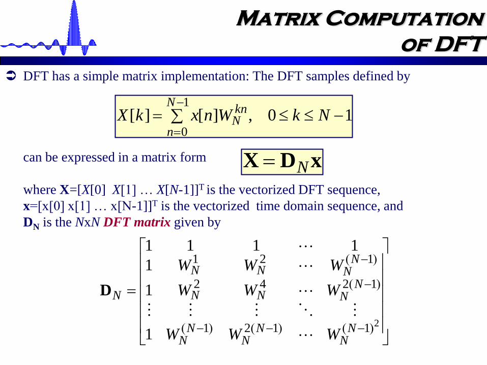
Matrix Computation

of DFT

DFT has a simple matrix implementation: The DFT samples defined by

can be expressed in a matrix form

where X=[X[0] X[1] … X[N-1]]T is the vectorized DFT sequence,

x=[x[0] x[1] … x[N-1]]T is the vectorized time domain sequence, and

DN is the NxN DFT matrix given by

10,][][1

0

NkWnxkXN

n

knN

xDX N

21121

1242

121

1

1

1

1111

)()()(

)(

)(

NN

NN

NN

NNNN

NNNN

N

WWW

WWW

WWW

D



Matrix Computation

of IDFT

• Likewise, the IDFT relation given by

can be expressed in matrix form as

where DN-1 is the NxN IDFT matrix

10,][][1

0

NnWkXnxN

k

nkN

XDx1 N

21121

1242

121

1

1

1

1

1111

)()()(

)(

)(

NN

NN

NN

NNNN

NNNN

N

WWW

WWW

WWW

D

*NN

NDD

11 Note that DFT and IDFT matrices

are related to each other



In Matlab

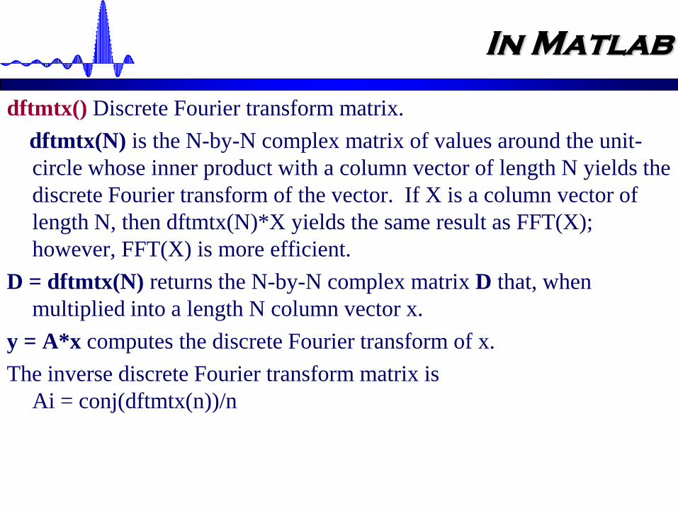
dftmtx() Discrete Fourier transform matrix.

dftmtx(N) is the N-by-N complex matrix of values around the unit-

circle whose inner product with a column vector of length N yields the

discrete Fourier transform of the vector. If X is a column vector of

length N, then dftmtx(N)*X yields the same result as FFT(X);

however, FFT(X) is more efficient.

D = dftmtx(N) returns the N-by-N complex matrix D that, when

multiplied into a length N column vector x.

y = A*x computes the discrete Fourier transform of x.

The inverse discrete Fourier transform matrix is

Ai = conj(dftmtx(n))/n



DTFT DFT

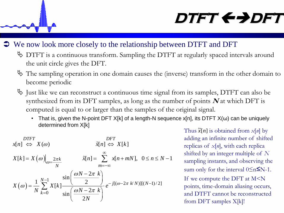
We now look more closely to the relationship between DTFT and DFT

DTFT is a continuous transform. Sampling the DTFT at regularly spaced intervals around

the unit circle gives the DFT.

The sampling operation in one domain causes the (inverse) transform in the other domain to

become periodic

Just like we can reconstruct a continuous time signal from its samples, DTFT can also be

synthesized from its DFT samples, as long as the number of points N at which DFT is

computed is equal to or larger than the samples of the original signal.

• That is, given the N-point DFT X[k] of a length-N sequence x[n], its DTFT X(ω) can be uniquely

determined from X[k]

2

1[( 2 / )][( 1) / 2]

0

[ ] ( ) [ ] [ ]

[ ] [ ] [ ], 0 1

2sin

1 2[ ]

2sin

2

DTFT DFT

k

mN

Nj k N N

k

x n X x n X k

X k X x n x n mN n N

N k

X X k eN kN

N

Thus is obtained from x[n] by

adding an infinite number of shifted

replicas of x[n], with each replica

shifted by an integer multiple of N

sampling instants, and observing the

sum only for the interval 0≤n≤N-1.

If we compute the DFT at M<N

points, time-domain aliasing occurs,

and DTFT cannot be reconstructed

from DFT samples X[k]!

][~ nx



While the DFT allows us to compute the discrete frequency response

of a discrete signal using a computer,

this process would have never become as influential as it is,

with as many applications as it has,

if it weren’t for the …



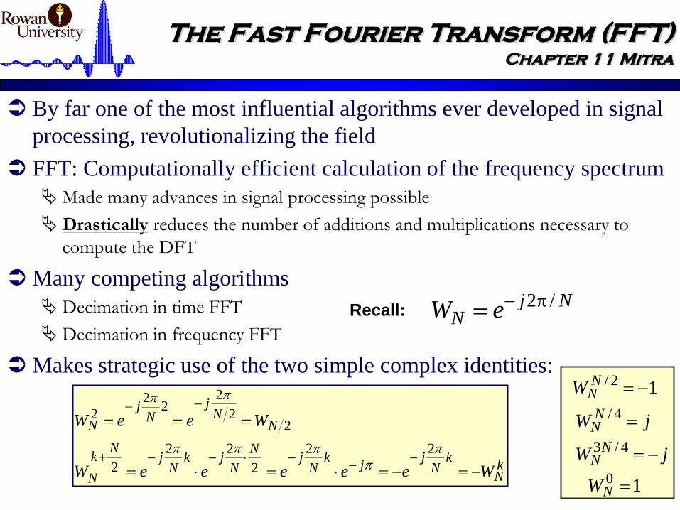
The Fast Fourier Transform (FFT)

Chapter 11 Mitra

By far one of the most influential algorithms ever developed in signal

processing, revolutionalizing the field

FFT: Computationally efficient calculation of the frequency spectrum

Made many advances in signal processing possible

Drastically reduces the number of additions and multiplications necessary to

compute the DFT

Many competing algorithms

Decimation in time FFT

Decimation in frequency FFT

Makes strategic use of the two simple complex identities:

kN

kN

jj

kN

jN

Njk

Nj

Nk

N

NN

jN

j

N

WeeeeeW

WeeW

22

2

22

2

22

22

2

2

10 NW

12/ NNW

jW NN 4/

jW NN 4/3

NjN eW /2Recall:



Computational

Complexity of DFT

Q: How many multiplications and additions are needed to compute DFT?

Note that for each “k” we need N complex multiplications, and N-1 complex

additions (WNkn) does not depend on x[n], and hence can be precomputed and saved in a table

Each complex multiplication is four real multiplications and two real additions

A complex addition requires two real additions

So for N values of “k”, we need N*N complex multiplications and N*(N-1) complex

additions

• This amounts to N2 complex multiplications and N*(N-1)~N2 (for large N) complex additions

• N2 complex multiplications: 4N2 real multiplications and ~2N2 real additions

• N2 complex additions: 2N2 real additions

A grand total of 4N2 real multiplications and 4N2 real additions:

• The computational complexity grows with the square of the signal size.

• This computational complexity is referred to as O(N2), also called, order of N2

• For , say 1000 point signal: 4,000,000 multiplications and 4,000,000 additions: OUCH!

1

0

, 0 1N

nk

N

n

X k x n W k N[ ] [ ]



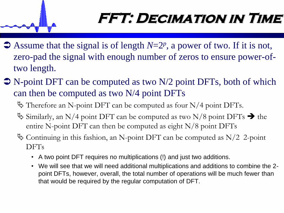
FFT: Decimation in Time

Assume that the signal is of length N=2p, a power of two. If it is not,

zero-pad the signal with enough number of zeros to ensure power-of-

two length.

N-point DFT can be computed as two N/2 point DFTs, both of which

can then be computed as two N/4 point DFTs

Therefore an N-point DFT can be computed as four N/4 point DFTs.

Similarly, an N/4 point DFT can be computed as two N/8 point DFTs the

entire N-point DFT can then be computed as eight N/8 point DFTs

Continuing in this fashion, an N-point DFT can be computed as N/2 2-point

DFTs

• A two point DFT requires no multiplications (!) and just two additions.

• We will see that we will need additional multiplications and additions to combine the 2-

point DFTs, however, overall, the total number of operations will be much fewer than

that would be required by the regular computation of DFT.



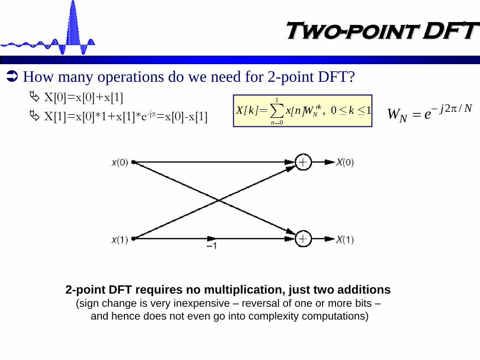
Two-point DFT

How many operations do we need for 2-point DFT?

X[0]=x[0]+x[1]

X[1]=x[0]*1+x[1]*e-jπ=x[0]-x[1]

1

0

, 0 1nk

N

n

X k x n W k

2-point DFT requires no multiplication, just two additions (sign change is very inexpensive – reversal of one or more bits –

and hence does not even go into complexity computations)

NjN eW /2[ ] [ ]



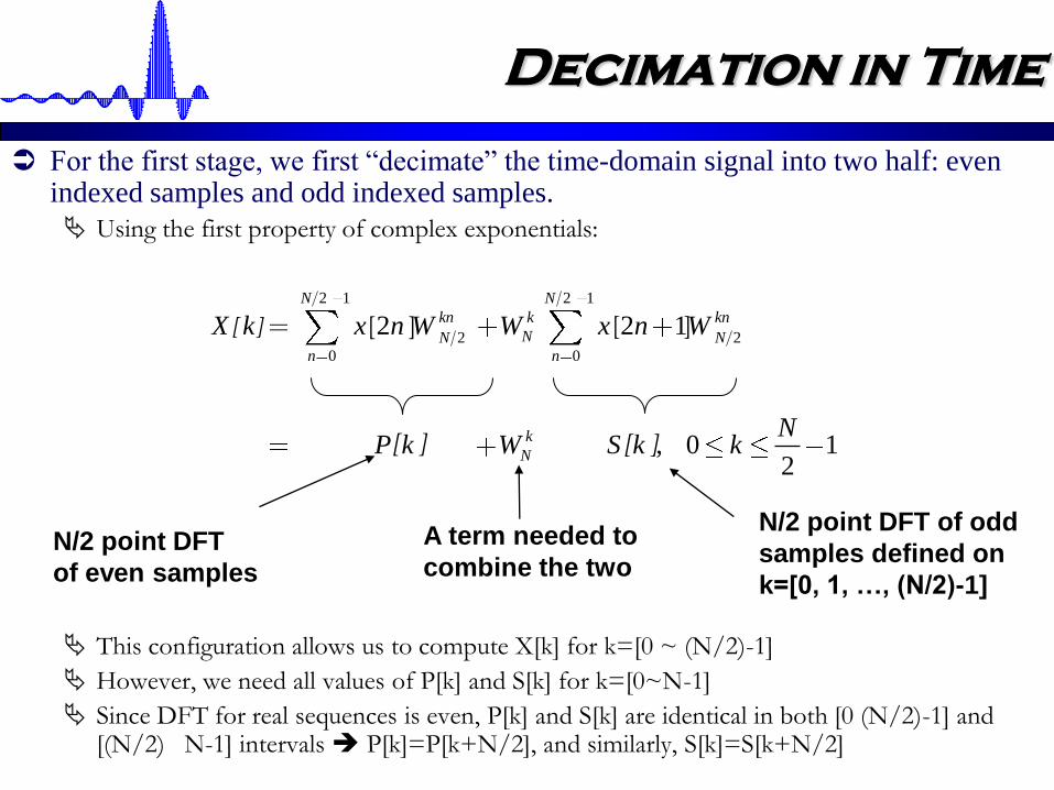
Decimation in Time

For the first stage, we first “decimate” the time-domain signal into two half: even indexed samples and odd indexed samples.

Using the first property of complex exponentials:

This configuration allows us to compute X[k] for k=[0 ~ (N/2)-1]

However, we need all values of P[k] and S[k] for k=[0~N-1]

Since DFT for real sequences is even, P[k] and S[k] are identical in both [0 (N/2)-1] and [(N/2) N-1] intervals P[k]=P[k+N/2], and similarly, S[k]=S[k+N/2]

2 1 2 1

2 2

0 0

2 2 1

, 0 12

N N

kn k kn

NN N

n n

k

N

X k x n W W x n W

NP k W S k k

N/2 point DFT

of even samples

N/2 point DFT of odd

samples defined on

k=[0, 1, …, (N/2)-1]

A term needed to

combine the two

[ ] [ ] [ ]

[ ] [ ]



2 2

[ ] [ ] [ ] 0 12

[ ] [ ] [ ] [ ] [ ] [ ] 0 12 2 2 2 2

k

N

k N k N

N N

NX k P k W S k k

N N N N NX k P k W S k X k P k W S k k

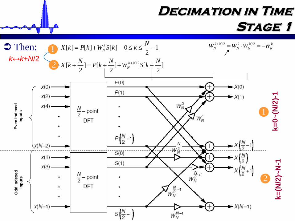
Decimation in Time

Stage 1

Then:

k=

0~

(N/2

)-1

k=

(N/2

)~N

-1

Ev

en

in

dexed

inp

uts

Od

d in

dexed

inp

uts

2 2k N k N k

N N N NW W W W

k↔k+N/2



The Butterfly Process

The basic building block in this implementation can be represented by the butterfly process.

Two multiplications & two additions

But we can do even better, just by moving the multiplier before the node S[k]

Reduced butterfly

1 multiplication and two additions !

We need N/2 reduced butterflies in stage 1 to connect the even and odd N/2 point DFTs

A total of (N/2) multiplications and 2*(N/2)=N additions

P[k]: Even indexed samples

S[k]: Odd indexed

samples



Stage 1 FFT

kNW

2

2

z-1

(N/2)-point

DFT

(N/2)-point

DFT][nx ][kX

][nxeven

][nxodd

][kP

kNW

][kS

kNW

1

]2

[N

kX

(N/2)2 multiplications+

(N/2)2 additions

(N/2)2 multiplications+

(N/2)2 additions

The butterfly

(N/2) mult. & N additions

RP



Stage 2…& 3…&4…

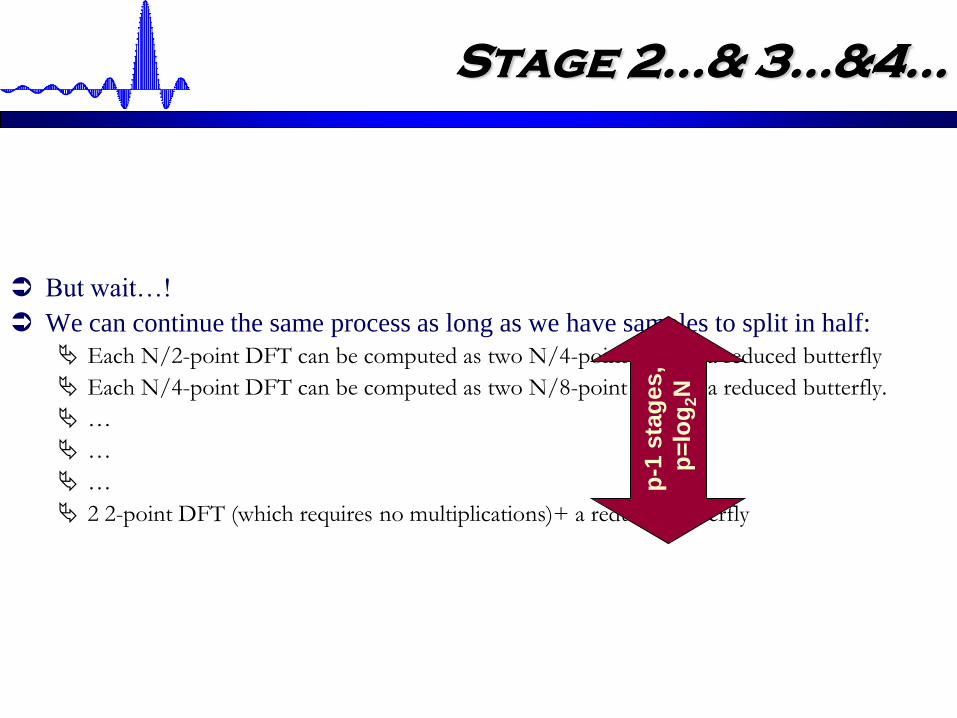
But wait…!

We can continue the same process as long as we have samples to split in half:

Each N/2-point DFT can be computed as two N/4-point DFT + a reduced butterfly

Each N/4-point DFT can be computed as two N/8-point DFT + a reduced butterfly.

…

…

…

2 2-point DFT (which requires no multiplications)+ a reduced butterfly

p-1

sta

ge

s,

p=

log

2N



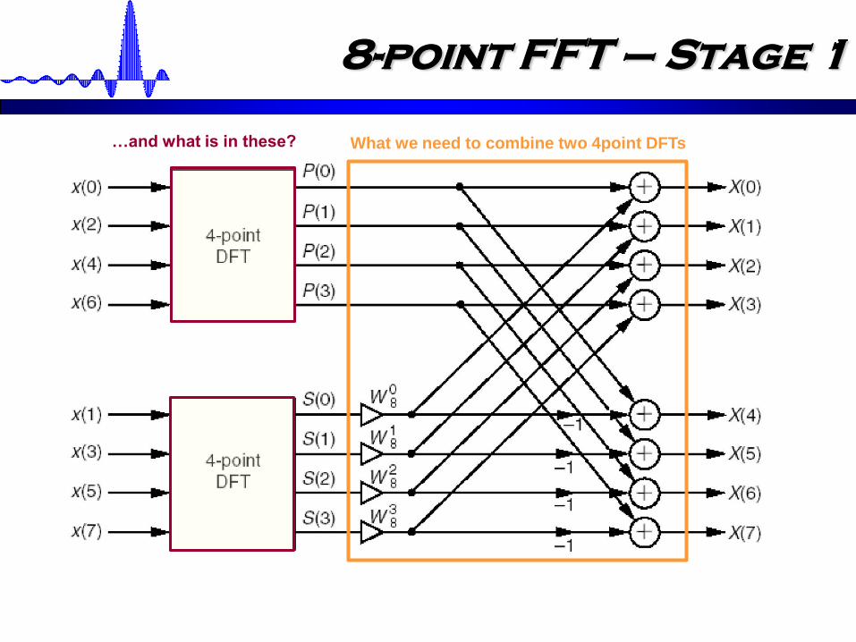
8-point FFT – Stage 1

What we need to combine two 4point DFTs…and what is in these?



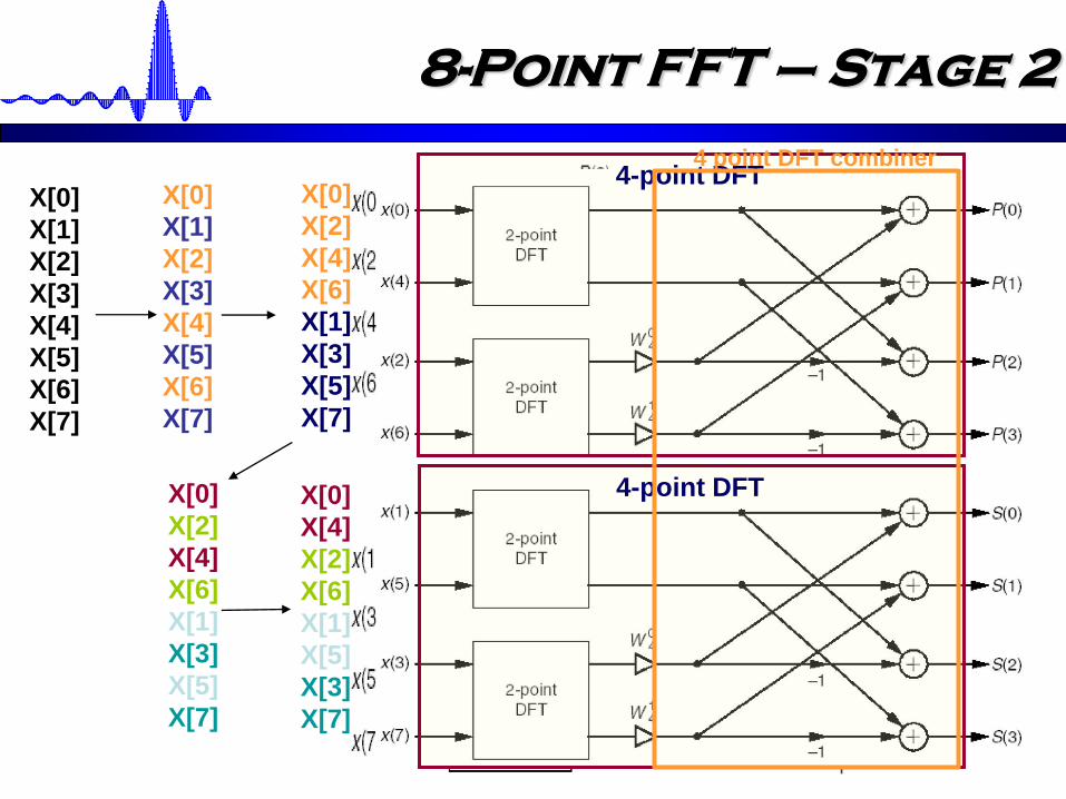
8-Point FFT – Stage 2

X[0]

X[2]

X[4]

X[6]

X[1]

X[3]

X[5]

X[7]

X[0]

X[2]

X[4]

X[6]

X[1]

X[3]

X[5]

X[7]

X[0]

X[4]

X[2]

X[6]

X[1]

X[5]

X[3]

X[7]

4-point DFT

4-point DFT

X[0]

X[1]

X[2]

X[3]

X[4]

X[5]

X[6]

X[7]

X[0]

X[1]

X[2]

X[3]

X[4]

X[5]

X[6]

X[7]

4 point DFT combiner




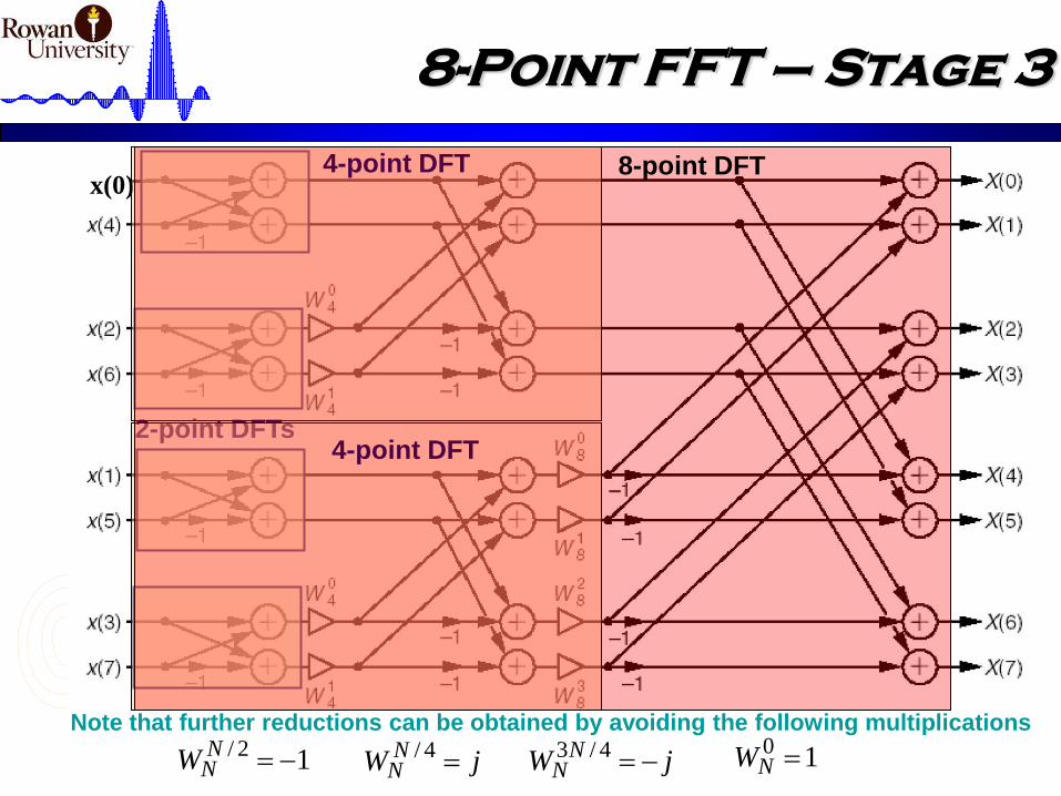
8-Point FFT – Stage 3

x(0)

Note that further reductions can be obtained by avoiding the following multiplications

10 NW12/ NNW jW N

N 4/ jW NN 4/3

2-point DFTs4-point DFT

4-point DFT 8-point DFT



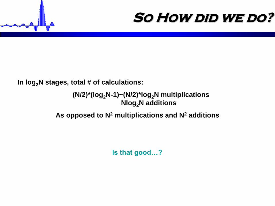
So How did we do?

In log2N stages, total # of calculations:

(N/2)*(log2N-1)~(N/2)*log2N multiplications

Nlog2N additions

As opposed to N2 multiplications and N2 additions

FFT: 5,120 multiplications and additions

For N=4096 DFT:16,777,216 multiplications and additions

Is that good…?



Decimation in Frequency

Just like we started with time-domain samples and decimated them in

half, we can do the same thing with frequency samples:

Compute the even indexed spectral samples k=0, 2, 4,…, 2N-1 and odd indexed

spectral components k=1, 3, 5, …, 2N-2 separately.

Then further divide each by half to compute X[k] for 0, 4, 8,… and 2, 6, 10, … as

well as 1, 5, 9, … and 3, 7, 11 …separately

Continuing in this manner, we can reduce the entire process to a series of 2-point

DFTs.



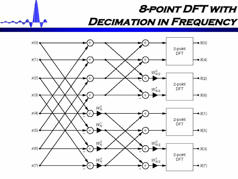
8-point DFT with

Decimation in Frequency



Filtering Streaming Data

In most real-world applications, the filter length is actually rather

small (typically, N<100); however, the input signal is obtained as a

streaming data, and therefore can be very long.

To calculate the output of the filter, we can

a) Wait until we receive all the data, and then do a full linear convolution of length

N filter and length M x[n], where M>>>>N y[n]=x[n]*h[n]

b) We can use the DFT based method y[n]=IDFT(X[k].H[k]), but we still

need to wait for the entire data to arrive to calculate X[k]

In either case, the calculation is very long, expensive, and need to

wait for the entire data to arrive.

Can we just process the data in batches, say 1000 samples at a time,

and then concatenate the results…?



What Happened…?

An example:

h[n]=[1 2 3 2 1]; (a short filter)

x[n]=[1 2 3 4 5 -1 -2 4 5 6 4 -2 -3 4 3 2 5 6 4 -1 -4 2 4 5 -1 2 3 4 -2 2 3 4 5 6 -2 1 2 3 1 -1 ]

1 1.5 2 2.5 3 3.5 4 4.5 50

2

4Short, length 5 filter h[n]

0 5 10 15 20 25 30 35 40-10

0

10Long, length 40 signal

0 5 10 15 20 25 30 35 40 45-50

0

50Filtered signal obtained in one convolution, length=40+5-1=44

0 10 20 30 40 50 60 70-50

0

50Filtered signal obtained as concatenation of individual segments, length=...?

h=[1 2 3 2 1]; % Some short filter N=5;

x=[1 2 3 4 5 -1 -2 4 5 6 4 -2 -3 4 3 2 5 6 4 -1 -4 ...

2 4 5 -1 2 3 4 -2 2 3 4 5 6 -2 1 2 3 1 -1]; % M=40

y=conv(x, h); % regular convolution Length N+M-1

%Let's divide the long x[n] into smaller segments and

calculate the convolution of each segment

x1=x(1:5); y1=conv(x1, h);

x2=x(6:10); y2=conv(x2, h);

x3=x(11:15); y3=conv(x3, h);

x4=x(20:25); y4=conv(x4, h);

x5=x(21:30); y5=conv(x5, h);

x6=x(31:35); y6=conv(x6, h);

x7=x(36:40); y7=conv(x7, h);

% Now add those segments together

y_batch=[y1 y2 y3 y4 y5 y6 y7];

%and compare to the original convolution

subplot(411); stem(h, 'filled'); grid

title('Short, length 5 filter h[n]')

subplot(412); stem(x, 'filled'); grid

title('Long, length 40 signal')

subplot(413); stem(y, 'filled'); grid

title(‘Single convolution, length=40+5-1=44')

subplot(414); stem(y_batch, 'filled'); grid

title(‘Concatenation of individual segments, length=...?')



y

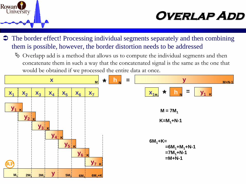
Overlap Add

The border effect! Processing individual segments separately and then combining

them is possible, however, the border distortion needs to be addressed

Overlapp add is a method that allows us to compute the individual segments and then

concatenate them in such a way that the concatenated signal is the same as the one that

would be obtained if we processed the entire data at once.

x1 x2 x3 x4 x5 x6 x7

y2

y3

y4

y5

y6

y7

* =

* =

x M hN

yM+N-1

x1M1

hN

y1 K

y1 K

K=M1+N-1K

K

K

K

K

K

M1 2M1 3M1 5M1 6M1 6M1+K

M = 7M1

6M1+K=

=6M1+M1+N-1

=7M1+N-1

=M+N-1RP



Example (Cont.)

So, here are the

individual segments

ordered in an

overlap-add format

0 5 10 15 20 25 30 35 40 450

20

40

0 5 10 15 20 25 30 35 40 45-50

0

50

0 5 10 15 20 25 30 35 40 450

10

20

0 5 10 15 20 25 30 35 40 45-50

0

50

0 5 10 15 20 25 30 35 40 45-50

0

50

0 5 10 15 20 25 30 35 40 450

10

20

0 5 10 15 20 25 30 35 40 45-50

0

50

0 5 10 15 20 25 30 35 40 45-20

0

20

OVERLAPP ADD

M=length(x); %Length of the original signal

M1=length(x1); % Length of each batch

N=length(h); %Length of the filter

K=length(y1); %Length of each filtered batch

L=M+N-1; %Length of the desired convolution

O=K-M1; % Amount of overlap

Y1=[zeros(1, 0*M1) y1 zeros(1, L-(1*M1)-O)];








Y=Y1+Y2+Y3+Y4+Y5+Y6+Y7+Y8;



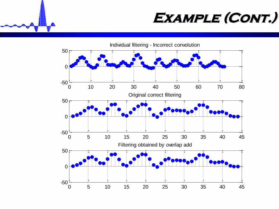
Example (Cont.)

0 10 20 30 40 50 60 70 80-50

0

50Individual filtering - Incorrect convolution

0 5 10 15 20 25 30 35 40 45-50

0

50Original correct filtering

0 5 10 15 20 25 30 35 40 45-50

0

50Filtering obtained by overlap add



Exercise

Something to ponder about:

Considering that DFT and IDFT equations are so similar to each other, one may

wonder whether IDFT can be calculated by using the DFT formulation itself. The

answer is a not-so-surprising, YES!

The original signal x[n] can be reconstructed from its DFT coefficients X[k],

simply by taking the DFT of X[k] again(!), with some minor modifications.

Find out how this can be done. This will be a bonus question in the future.



discrete fourier transform - kasetsart universityjan/dsp/note/lecture-08-2-r05.pdf · discrete...

Documents