discrete-time system analysis using the z...
TRANSCRIPT

Discrete-Time System Analysis Using the z-Transform
S Wongsa
11
S Wongsa
Dept. of Control Systems and Instrumentation Engineering,
KMUTT
Overview
� z-Transform
� Definition
� Some properties
� The Inverse z-Transform
� Partial fraction expansion
22
� Applications of z-Transform
� Solution of Linear Difference Equations
� Characterisation of Discrete-Time LTI Systems
- Transfer function, zero-pole-gain
- Causality, Stability

z-Transform
Given a DT signal x[n], its z-transform is defined as
∑∞
−∞=
−=n
nznxzX ][)(
where z is a complex variable , called the z-transform variable.
∑∞
=
−=0
][)(n
nznxzX
One-sided / Unilateral z-TransformTwo-sided / Bilateral z-Transform
ωjrez =
33
� The notation
)(][ zXnx ⇔
� If
))...()((
))...()(()(
21
21
p
z
n
n
pzpzpz
zzzzzzzX
−−−
−−−=
- zi, i=1,…,nz, are called the zeros of X(z).
- pi, i=1,…,np, are called the poles of X(z).
The Region of Convergence
• The set of values of z for which the sum converges and X(z) exists is called
the region of convergence or ROC.
EXAMPLE :
,][z
nuan ⇔ |||| az >
Causal exponential
44
,][az
znuan
−⇔ |||| az >
|||| az <
Left-sided exponential
,]1[az
znuan
−⇔−−−

Some Common z-Transform Pairs
55
The Inverse z-Transform
∫ −=C
n dzzzXj
nx 1)(2
1][
π
where C is a closed contour that includes all poles of X(z).
Definition
66
� If X(z) is in the rational form, i.e. X(z)=B(z)/A(z), we can compute the inverse
z-transform using the partial fraction expansion.
� But doing it requires integration in the complex plane and it is rarely used in engineering
practice.

The Inverse z-Transform
• Partial Fraction Expansion
Given
))...()((
))...()(()(
21
21
p
z
n
n
pzpzpz
zzzzzzzX
−−−
−−−=
• It is assumed that nz ≤≤≤≤ np (proper form) before carrying out the next step.
If this is not the case, carry out the long division until it is.
77
i) If the poles are distinct and are all nonzero:
expand X(z) into a sum of terms
p
p
n
n
pz
zc
pz
zcczX
−++
−+= ...)(
1
10
where
00 |)( == zzXc
ipzi
i zXz
pzc =
−= |)(
)(for pni ≤≤1
The Inverse z-Transform
• Partial Fraction Expansion
EXAMPLE : Distinct poles
2
102)(
2
2
−−+
=zz
zzX
345)( ++−=zz
zX ][)2(3][)1(4][5][ nununnx nn +−+−= δ
88
23
145)(
−+
++−=
z
z
z
zzX ][)2(3][)1(4][5][ nununnx nn +−+−= δ
...20]3[,16]2[,2]1[,2]0[ ==== xxxx

The Inverse z-Transform
• Partial Fraction Expansion
EXAMPLE : Complex poles
)2)(1(
1
2
1)(
2
3
23
3
−+++
=−−−
+=
zzz
z
zzz
zzX
• The poles of X(z) are . 2,866.05.0 j±−
99
• Expanding X(z) gives
2
643.0
866.05.0
)0825.0429.0(
866.05.0
)0825.0429.0(5.0)(
−+
−+−
+++
++−=
z
z
jz
zj
jz
zjzX
• The inverse z-transform of X(z) is
][)2(643.0][89.103
4cos874.0][5.0][ nununnnx n+
++−= oπδ
The Inverse z-Transform
• Partial Fraction Expansion
ii) Repeated poles:
If the pole p1 is repeated r times and the other np-r poles are distinct,
pnr
r
r
pz
zc
pz
zc
pz
zc
pz
zc
pz
zcczX
−++
−+
−++
−+
−+= + ...
)(...
)()( 1
2
210
1010
pnr
r pzpzpzpzpzczX
−++
−+
−++
−+
−+=
+
...)(
...)(
)(11
2
11
0
where
1
)()(
!
11
pz
r
i
i
irz
zXpz
dz
d
ic
=
−
−= for 1,...,0 −= ri
• The constants are computed in the same way as
in the distinct pole case.pnrr cccc ,..., and 2,10 ++

The Inverse z-Transform
• Partial Fraction Expansion
EXAMPLE : Repeated poles
)1()1(
26
1
26)(
2
23
23
23
+−−+
=+−−−+
=zz
zzz
zzz
zzzzX
75.05.325.5 zzz
1111
1
75.0
)1(
5.3
1
25.5)(
2 ++
−+
−=
z
z
z
z
z
zzX
][)1(75.0][5.3][25.5][ nunnununx n−++=
Some properties of the z-Transform
Properties Sequence1 z-transform
Linearity
Time shifting
)()( zbYzaX +][][ nbynax +
][ knx −
][ knx + ∑−
=
−−1
0
][)(k
i
ikk zixzXz
∑=
−− −+k
i
kik zixzXz1
][)(
1212
Scaling
Differentiation
Convolution
Initial value
Final value
theorem
1All sequences are causal.
][nxan )/( azX
∑∞
−∞=
−l
lnylx ][][ )()( zYzX
][nnx )(zXz &−
exists.limit theif ),(lim]0[ zXx z ∞→=
circle.unit theinside are )()1( of poles theif
),()1(limor )()1(lim][lim 1
11
zXz
zXzzXznx zzn
−
−−= −→→∞→
The Inverse z-Transform
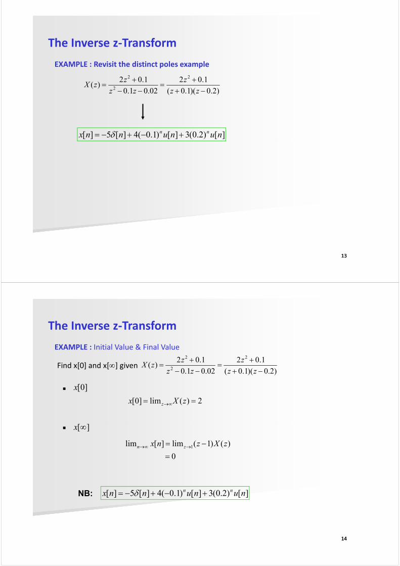
EXAMPLE : Revisit the distinct poles example
)2.0)(1.0(
1.02
02.01.0
1.02)(
2
2
2
−++
=−−
+=
zz
z
zz
zzX
][)2.0(3][)1.0(4][5][ nununnx nn +−+−= δ
1313
The Inverse z-Transform
EXAMPLE : Initial Value & Final Value
Find x[0] and x[∞] given
� ][∞x
�
2)(lim]0[ == ∞→ zXx z
]0[x
)2.0)(1.0(
1.02
02.01.0
1.02)(
2
2
2
−++
=−−
+=
zz
z
zz
zzX
1414
�
0
)()1(lim][lim 1
=
−= →∞→ zXznx zn
][∞x
][)2.0(3][)1.0(4][5][ nununnx nn +−+−= δNB:

The Inverse z-Transform
� Z-transform Partial Fraction Expansion Using MATLAB
Z-transform partial-fraction expansion can be computed using the MATLAB
command ‘residuez’ (X(z) in ascending powers of z-1)
02.01.0
1.02)(
2
2
−−+
=zz
zzX
21
2
02.01.01
1.02)( −−
−
−−+
=zz
zzX
1515
>> num=[2 0 0.1];
>> den=[1 -0.1 -0.02];
>> [r,p,k]=residuez(num,den)
r = 3
4
p = 0.2000
-0.1000
k = -5
11 2.01
13
1.01
145)( −− −
++
+−=zz
zX
2.03
1.045)(
−+
++−=
z
z
z
zzX
By calculation:
The Inverse z-Transform
• The Inverse z-Transform Using MATLAB
x =iztrans(X) is the inverse Z-transform of the scalar sym X with default
independent variable z.
02.01.0
1.02)(
2
2
−−+
=zz
zzX ][)2.0(3][)1.0(4][5][ nununnx nn +−+−= δ
1616
>> syms X x z
>> X=(2*z^2+0.1)/(z^2-0.1*z-0.02);
>> x=iztrans(X)
x =
3*(1/5)^n + 4*((-1/10))^n - 5*kroneckerDelta(n, 0)

Overview
� z-Transform
� Definition
� Some properties
� The Inverse z-Transform
� Partial fraction expansion
1717
� Applications of z-Transform
� Solution of Linear Difference Equations
� Characterisation of Discrete-Time LTI Systems
- Transfer function, zero-pole-gain
- Causality, Stability
Applications of z-Transform
Given the following difference equation
where y and x are the output and the input variables, respectively.
• Solution of linear difference equations
Mnxbn-xbnxb
Nnyanyanyany
M
N
][...]1[][
...][...]2[]1[][
10
21
−+++
+−−−−−−−=
1818
i) Taking z-transform to both sides and rearranging gives
)()(
)()(
...1
...)(
1
1
1
10 zXzA
zBzX
zaza
zbzbbzY
N
N
M
M =++++++
= −−
−−
ii) The solution of the difference equation is
y[n] = Z-1{Y(z)}
(If all initial conditions are zero)

Applications of z-Transform
EXAMPLE : Non-zero initial conditions
]1[][]2[1.0]1[7.0][ −−=−+−− nununynyny
If u[n] is the unit step and suppose that y[-2]=0,y[-1]=1, compute the output
response y[n].
( ) ( ) ( )]1[)()(]2[]1[)(1.0]1[)(7.0)( 1121 −+−=−+−++−+− −−−− uzUzzUyzyzYzyzYzzY
1919NB: ][ knx − ∑
=
−− −+k
i
kik zixzXz1
][)(
( ) 111
11.07.0)()1.07.01(
1
1
1
121 =−
−−
=+−++−−
−
−−−−
z
z
zzzYzz
121 1.07.1)()1.07.01( −−− −=+− zzYzz
Applications of z-Transform
EXAMPLE : Non-zero initial conditions
−=
−= 8.05.2
)1.07.1()(
zzzzzY
121 1.07.1)()1.07.01( −−− −=+− zzYzz
2020
−
−−
=+−
=2.0
8.05.0
5.21.07.0
)(2 zzzz
zY
][))2.0(8.0)5.0(5.2(][ nuny nn −=

Applications of z-Transform
• Solution of linear difference equations by MATLAB
For N ≥ M, the output of the system described by
can be found using the MATLAB command ‘filter’.
y=filter(b,a,x,zi) .
Mnxbn-xbnxb
Nnyanyanyany
M
N
][...]1[][
...][...]2[]1[][
10
21
−+++
+−−−−−−−=
2121
y=filter(b,a,x,zi) .
b = [b0 b1 … bM]
a = [1 a1 a2 … aN ]
x is the input vector.
zi is the initial condition vector = [zi(1) zi(2) … zi(N)] and
where
)1()(
)1(...)2()1()2(
)(...)2()1()1(
32
21
−−=
+−−−−−−−=
−−−−−−−=
yaNzi
Nyayayazi
Nyayayazi
N
N
N
M
Applications of z-Transform
• NB
The initial condition vector can be formulated by using the command ‘filtic’
zi=filtic(b,a,y,x) .
b = [b0 b1 … bM]
a = [1 a a … aN ]
where
2222
a = [1 a1 a2 … aN ]
The vectors x and y contain the most recent input or output first, and oldest input
or output last.
]][],...,2[],1[[
][],...,2[],1[[
Nyyyy
Mxxxx
−−−=
−−−=
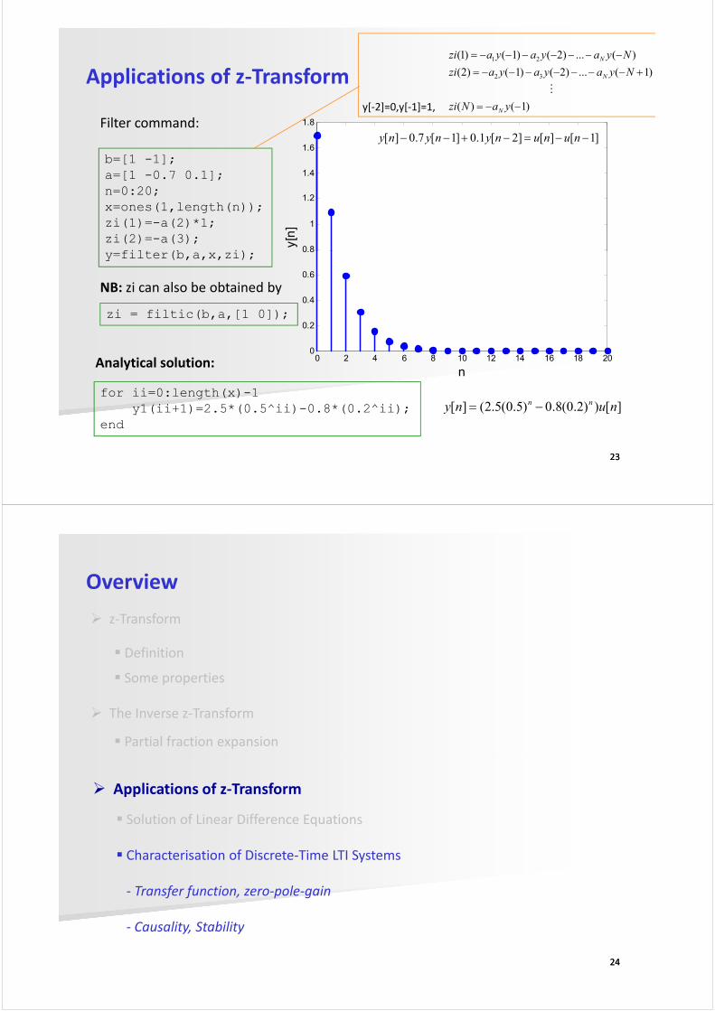
Applications of z-Transform
b=[1 -1];
a=[1 -0.7 0.1];
n=0:20;
x=ones(1,length(n));
zi(1)=-a(2)*1;
zi(2)=-a(3);
y=filter(b,a,x,zi);
Filter command:
0.8
1
1.2
1.4
1.6
1.8
y[n]
y[-2]=0,y[-1]=1, )1()(
)1(...)2()1()2(
)(...)2()1()1(
32
21
−−=
+−−−−−−−=
−−−−−−−=
yaNzi
Nyayayazi
Nyayayazi
N
N
N
M
]1[][]2[1.0]1[7.0][ −−=−+−− nununynyny
2323
y=filter(b,a,x,zi);
Analytical solution:
for ii=0:length(x)-1
y1(ii+1)=2.5*(0.5^ii)-0.8*(0.2^ii);
end
0 2 4 6 8 10 12 14 16 18 200
0.2
0.4
0.6
0.8
n
zi = filtic(b,a,[1 0]);
NB: zi can also be obtained by
][))2.0(8.0)5.0(5.2(][ nuny nn −=
Overview
� z-Transform
� Definition
� Some properties
� The Inverse z-Transform
� Partial fraction expansion
2424
� Applications of z-Transform
� Solution of Linear Difference Equations
� Characterisation of Discrete-Time LTI Systems
- Transfer function, zero-pole-gain
- Causality, Stability

Discrete-Time LTI (Linear-Time Invariant) Systems
� Linearity : defined by the principle of superposition
LTI x1[n] y1[n] LTI x2[n] y2[n]
2525
LTI ax1[n]+bx2[n] ay1[n]+by2[n]
Scaling & additivity
properties
Discrete-Time LTI (Linear-Time Invariant) Systems
� Time Invariant
LTI x[n] y[n] LTI x[n-k] y[n-k]
2626

Discrete-Time LTI Systems
2727
h[n] is the impulse response function. The z-transform of h[n] is referred to as the
transfer function.
)(
)()(
zX
zYzH =
EXAMPLE For the unit impulse response
( ) ][])5.0(5.0[][ nunh nn ⋅−+=
, find the transfer function H(z).
( ) ]}[)5.0(][5.0{)( nunuZzH nn ⋅−+⋅=
Solution
2828
( ) ]}[)5.0(][5.0{)( nunuZzH ⋅−+⋅=
25.0
2
5.05.0)(
2
2
−=
++
−=
z
z
z
z
z
zzH

Difference Equation to Transfer Function
• Given a difference equation
Mnxbn-xbnxb
Nnyanyanyany
M
N
][...]1[][
...][...]2[]1[][
10
21
−+++
+−−−−−−−=
2929
If all initial conditions are zero, we find the transfer function to be
)(
)(
...1
...)(
1
1
1
10
zA
zB
zaza
zbzbbzH
N
N
M
M =++++++
= −−
−−
Applications of z-Transform
EXAMPLE :
]1[][]2[1.0]1[7.0][ −−=−+−− nununynyny
Find the transfer function of the difference equation above.
1.07.0
)1(
1.07.01
1
)(
)()(
)()()(1.0)(7.0)(
221
1
121
+−−
=+−
−==
−=+−
−−
−
−−−
zz
zz
zz
z
zU
zYzH
zUzzUzYzzYzzY
3030
1.07.01.07.01)( 221 +−+− −− zzzzzU

Gain, Poles & Zeros
))...()((
))...()(()(
21
21
p
z
n
n
pzpzpz
zzzzzzKzH
−−−
−−−=
A transfer function can be factored into
• K is called the system gain.
• zi, i=1,…,nz is called the system zeros.
3131
• zi, i=1,…,nz is called the system zeros.
• pi, i=1,…,np is called the system poles.
x
5.0)(
+=z
zzH
Characterisation of Discrete-Time LTI Systems
� Causality
� A system is causal if output at time n depends only on present and past inputs but
not on future.
� For real-time processing the system needs to be causal.
EXAMPLE
3232
]1[][][ −+= nxnxny
]1[][][ ++= nxnxny
Causal system
Noncausal system

Characterisation of Discrete-Time LTI Systems
� Causality condition
For a causal discrete-time LTI system, we have
0,0][ <= nnh
3333Pictures from Steven W. Smith, The Scientist and Engineer's Guide to Digital Signal Processing.
Characterisation of Discrete-Time LTI Systems
� Stability
� A system is stable in the bounded-input, bounded-output (BIBO) sense if and
only if every bounded input sequence produces a bounded output sequence.
When |x[n]| < B , if |y[n]|<∞, the system is stable.
� It can be shown that a discrete-time LTI system is BIB0 stable if its
3434
� It can be shown that a discrete-time LTI system is BIB0 stable if its
impulse response is absolutely summable, that is,
∞<∑∞
−∞=n
nh ][

Proof: Stability
We get
2121 zzzz +≤+
zzzz =
3535
using property that
If the impulse response is absolutely summable, i.e.
Then , i.e. y[n] is bounded.∞<][ny
2121 zzzz =
� Stability
A discrete-time system is BIBO stable, if and only if
pi nip ,...,1for 1|| =<
� Stability condition
Characterisation of Discrete-Time LTI Systems
3636
pnppp ,...,, 21where are the poles of H(z).

� Marginal Stability
A discrete-time system is marginally stable if and only if
and poles dnonrepeate allfor 1|| ≤ip
� Marginal Stability Condition
Characterisation of Discrete-Time LTI Systems
3737
poles. repeated allfor 1|| <i
i
p
Given a first-order system with a pole at z = a,
az
zzH
−=)( nanh =][
EXAMPLE
Characterisation of Discrete-Time LTI Systems
3838
0 5 100
0.2
0.4
0.6
0.8
1
n
a=1.0
X
Stable Marginally Stable Unstable