AQUACULTURE ENVIRONMENT INTERACTIONSAquacult Environ Interact

Vol. 8: 463–480, 2016doi: 10.3354/aei00192

Published August 23

INTRODUCTION

Increased environmental concerns about therelease of effluents from open-water finfish culturehave prompted monitoring and modelling to assessthe potential negative impacts (Holmer et al. 2008)and approaches to utilize waste nutrients, such asIntegrated Multi-Trophic Aquaculture (IMTA; Chopinet al. 2012). In most major fish-producing jurisdic-tions, cage-based aquaculture is primarily monitoredthrough benthic environmental conditions (Wilson et

al. 2009), with a few exceptions such as Malta (Hol -mer et al. 2008) and the Canadian Great Lakes (Boydet al. 2001). Likewise, the majority of aquacultureenvironmental impact studies focus on the depositionof organic aquaculture wastes and the associatedeffects to benthic faunal and sediment biochemicalprocesses (e.g. Karakassis et al. 2000, Kutti et al.2007, Holmer et al. 2008, Borja et al. 2009, Chopin etal. 2012, Valdemarsen et al. 2012). Pelagic (horizon-tal) dispersion of organic particles and inorganicnutrients at fish culture operations is less well under-

© The authors 2016. Open Access under Creative Commons byAttribution Licence. Use, distribution and reproduction areunrestricted. Authors and original publication must be credited.

Publisher: Inter-Research · www.int-res.com

*Corresponding author: henrice.jansen@wur.nl

AS WE SEE IT

Discrete water quality sampling at open-wateraquaculture sites: limitations and strategies

H. M. Jansen1,2,*, G. K. Reid3,4, R. J. Bannister1, V. Husa1, S. M. C. Robinson4, J. A. Cooper4, C. Quinton5, Ø. Strand1

1Institute of Marine Research, Nordnesgaten 50, 5817 Bergen, Norway2Wageningen Marine Research, Korringaweg 7, 4401 NT, Yerseke, The Netherlands

3Canadian Integrated Multi-Trophic Aquaculture Network, University of New Brunswick, New Brunswick, E2L 4L5, Canada 4St. Andrews Biological Station, Fisheries and Oceans Canada, St. Andrews, New Brunswick, E5B 2L9, Canada

5Animal Biosciences, University of Guelph, Guelph, Ontario, N1G 2W1, Canada

ABSTRACT: While environmental performance of cage-based aquaculture is most often moni-tored through benthic conditions, there may also be requirements that necessitate discrete,pelagic sampling. In the pelagic realm, adequately capturing the spatial and temporal dynamicsof interest and attributing causality to aquaculture processes can be extremely challenging. Con-ditions are seldom ideal, and data adequacy concerns of discrete samples collected at open-wateraquaculture sites are not uncommon. Further exploration of these challenges is needed. Herein,we aim to explore considerations for study design, analysis, and data interpretation of discretepelagic sampling. As examples, we present 2 case studies where limited sampling occurred underconditions of complex pelagic dynamics. A Norwegian case study quantified particle abundancearound salmon farms, and aimed to highlight the effects of spatial−temporal variation on samplingdesign, the need for inclusion of companion parameters, and the benefits of a priori and a posteri-ori data interpretation strategies. A Canadian case study collected discrete samples to measureammonium concentrations with continuous current measurements at an Integrated Multi-TrophicAquaculture (IMTA) farm, to explore issues of complex hydrodynamics, reference site suitability,sampling resolution, data pooling, and post hoc power tests. We further discuss lessons learnedand the implications of study design, ambient conditions, physical processes, farm management,statistical analysis, companion parameters, and the potential for confounding effects. Pragmaticconsideration of these aspects will ultimately serve to better frame the costs and benefits of discrete pelagic sampling at open-water aquaculture sites.

KEY WORDS: Sampling design · Pelagic · IMTA · Nutrients · Cage aquaculture · Farm-scale

OPENPEN ACCESSCCESS

Aquacult Environ Interact 8: 463–480, 2016

stood and studied (Sará 2007a, Handå et al. 2012a,Husa et al. 2014). Nevertheless, there can be variousrequirements that necessitate pelagic sampling ofnutrients at fish cages. Farmers may require detailson nutrient plumes for species placement in IMTA,regulators may want to know the potential for hori-zontal dispersion, and models require data validation.

Soluble metabolic by-products of fish culture thatcan be measured in the water column include ammo-nium (NH4

+) and orthophosphate (PO43−) (Sará 2007b).

Respired carbon dioxide (CO2) is not normally meas-ured at fish cages, but trends are sometimes inferredthrough other water-quality proxies (Reid et al. 2006).Typically, nitrogen is the limiting nutrient in marinesystems (Howarth & Marino 2006), as is phosphorusin freshwater (Dillon & Rigler 1974). These limitingnutrients are still commonly measured through dis-crete water sample collection followed by wet chem-istry techniques, notwithstanding recent encourag-ing developments of in situ nutrient analysers (Araiet al. 2011, Wild-Allen & Rayner 2014). Though solu-ble nitrogen forms and phosphate are measurablewith in situ analysers, total phosphorus (TP) is not atpresent, and this is the recommended nutrient formfor aquaculture monitoring in freshwater due to thepotential for rapid cycling of soluble phosphorus(Hudson et al. 1999, Boyd et al. 2001). There are sev-eral practical and logistical issues involved in meas-uring pelagic nutrients at open-water aquaculturesites (Brooks et al. 2003, Macleod et al. 2004, Gao etal. 2005). The process of collecting a discrete pelagicwater sample is intuitively simple. However, collect-ing an appropriate amount of discrete samples intime and space to adequately capture the spatial andtemporal scale of interest, or to attribute cause andeffect relationships to aquaculture, evidently setslimits to such investigations. Ecosystem, farm type,hydrodynamics, site characteristics, and husbandrypractices represent complex sources of variation inthe quantification of aquaculture influences on water-column properties (Sará 2007b). Consequently, thesampling regimen necessary to acquire meaning -ful results may need to be intensive, prolonged, orimpractical.

It is common for the discrete data collected in thiscomplex environment to be influenced by confound-ing effects and undersampling, leading to difficultiesin applying inferential statistics and drawing conclu-sions. With this paper, we aim to emphasize some ofthe challenges encountered in pelagic data collectionby exploring the sampling requirements necessary toachieve meaningful results and by discussing severalapproaches to maximize information from limited

data sets. Several of the issues addressed here havebeen debated previously in the international litera-ture, but typically not in the context of open-wateraquaculture. We suggest that a practical discussionon the challenges of discrete pelagic sampling istherefore warranted to infer the cause and effect re -lationships of aquaculture. In this paper we first pres-ent Norwegian and Canadian case studies as exam-ples of the complex dynamics of pelagic samplingand possible strategies for analysing and interpretingless-than-ideal data sets. In the second part of thepaper we explore lessons learned, through a reviewof sampling design, sampling strategies, data analy-sis, and data interpretation. We thereby aim to guidefarm operators and researchers in the appropriateuse of discrete sampling methods to assess waterquality at open-water aquaculture sites based onpractical considerations.

TWO FARM-SCALE CASE STUDIES

Challenges related to sampling of fine particulatesat salmon farms in Norwegian stratified fjord

systems

Study objectives

It is relevant to quantify and understand the dy -namics of fine particulates at open-water fish farmsin the context of IMTA development when bivalvefilter-feeders are integrated with finfish (Brager et al.2016). This case study presents a short-term sam-pling program that defines the abundance of fineparticles in the water column. We thereby aim tohighlight considerations of spatial-temporal variationon sampling design, the need for inclusion of com-panion parameters, and the benefits of a priori and aposteriori strategies for data interpretation.

Sampling design and data analysis

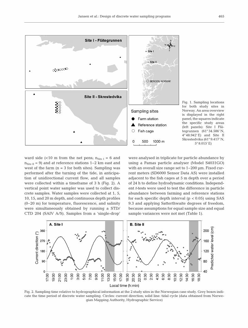
Field measurements were conducted at 2 large-scale Atlantic salmon farms in central Norway. Thestudy was carried out in September 2012, 2 mo afterthe farms were stocked with juvenile Atlantic salmonSalmo salar of ~100 g. Site I (Flåtegrunnen), con-sisted of 7 circular net pens situated in a row parallelto the dominant current direction, and at Site II(Skrestedvika) 2 rows of 5 cages were situated per-pendicular to the major current (Fig. 1). Sampleswere collected close to the fish net pens on the lee-

464

Jansen et al.: Design of discrete water sampling programs

ward side (<10 m from the net pens; nSite I = 6 andnSite II = 9) and at reference stations 1−2 km east andwest of the farm (n = 3 for both sites). Sampling wasperformed after the turning of the tide, in anticipa-tion of unidirectional current flow, and all sampleswere collected within a timeframe of 3 h (Fig. 2). Avertical point water sampler was used to collect dis-crete samples. Water samples were collected at 1, 5,10, 15, and 20 m depth, and continuous depth profiles(0−20 m) for temperature, fluorescence, and salinitywere simultaneously obtained by running a STD/CTD 204 (SAIV A/S). Samples from a ‘single-drop’

were analysed in triplicate for particle abundance byusing a Pamas particle analyser (Model S4031GO)with an overall size range set to 1−200 µm. Fixed cur-rent meters (SD6000 Sensor Data AS) were in stalledadjacent to the fish cages at 5 m depth over a periodof 24 h to define hydro dynamic conditions. Independ-ent t-tests were used to test the difference in particleabundance between farming and reference stationsfor each specific depth interval (p < 0.05) using SAS9.3 and applying Satterthwaite degrees of freedom,because assumptions for equal sample size and equalsample variances were not met (Table 1).

465

Fig. 1. Sampling locationsfor both study sites in Norway. An area overviewis displayed in the rightpanel; the squares indicatethe specific study areas(left panels): Site I Flå -tegrunnen (61° 34.586’ N,4° 48.942’ E) and Site IISkrestedvika (61° 9.417’ N,

5° 8.015’ E)

Fig. 2. Sampling time relative to hydrographical information at the 2 study sites in the Norwegian case study. Grey boxes indi-cate the time period of discrete water sampling. Circles: current direction; solid line: tidal cycle (data obtained from Norwe-

gian Mapping Authority, Hydrographic Service)

Aquacult Environ Interact 8: 463–480, 2016

Sampling execution and data interpretation

Even with the low fish biomass (0.72 kg m−3) presentat the start of the production cycle, enhanced particleabundance was observed close to the salmon seacages (Fig. 3A,D). At Site I differences in particle con-

centrations between the farm and ref-erence stations were most profound at5 m depth (Fig. 3A), and at Site II en-hancement of particle concentrationsat the farm stations was significant forall depth intervals except the surface(Fig. 3D). Furthermore, distinct stra -tification of the water column was observed in the upper 10−15 m(Fig. 3B,C,E,F), which is common inNorwegian fjord systems during sum-mer and early autumn (Sætre 2007). AtSite I, vertical profiles of companionparameters, such as temperature andsalinity, showed similarity betweenthe farming and reference stations(Fig. 3B,C). This suggests that the water body close to the farm was rep-resentative of the surrounding envi-ronment, and differences in particleabundance can be attributed to wasterelease from the farms. At Site II, how-ever, dissimilar profiles were observed(Fig. 3E,F) with the stratification occur-ring at 10 m depth at the reference sta-tion, while at the farming stationsstratification was observed at 15 m.This suggests that enhanced particle

abundance may also be related to factors other thanwaste release from the farm only. Explanations for thismight relate to (1) local hydrodynamic conditionsaround fish cages (spatial), (2) tidal influences duringthe sampling execution (temporal), or (3) the appro-priateness of reference sites.

466

Depth Sample Particle conc. t-test assumption df t p(m) (mean ± SD) for sample variance

Site I: Flategrunnen1 Farm 11501 ± 2401 Satterthwaite* 6.71 1.94 0.0950

Ref 9700 ± 704 Pooled 7 1.44 0.19245 Farm 9435 ±1913 Satterthwaite* 6.07 4.61 0.0036

Ref 5623 ± 473 Pooled 7 3.30 0.013210 Farm 4871 ± 1476 Satterthwaite* 6.62 2.41 0.0486

Ref 3279 ± 483 Pooled 7 1.78 0.118615 Farm 3247 ± 1800 Satterthwaite 5.44 1.13 0.3056

Ref 2397 ± 274 Pooled* 7 0.79 0.457520 Farm 3167 ± 922 Satterthwaite* 5.51 2.96 0.0280

Ref 2024 ± 150 Pooled 7 2.06 0.0778

Site II: Skrestedvika1 Farm 7675 ± 341 Satterthwaite* 2.42 0.18 0.8717

Ref 7609 ± 614 Pooled 10 0.24 0.81235 Farm 7721 ± 659 Satterthwaite* 8.78 3.73 0.0049

Ref 6706 ± 279 Pooled 10 2.53 0.030110 Farm 7585 ±1593 Satterthwaite* 8.78 6.24 0.0002

Ref 3418 ±621 Pooled 9 4.29 0.00215 Farm 5110 ± 1220 Satterthwaite* 9.47 6.85 <0.0001

Ref 2162 ± 242 Pooled 10 4.03 0.002420 Farm 2918 ± 546 Satterthwaite* 6.57 4.28 0.0042

Ref 1828 ± 308 Pooled 10 3.22 0.0091

Table 1. Paired comparisons (t-test) of particle concentrations between farmand reference (Ref) sites for the Norwegian case study. Statistical outputincludes both results for assumptions of unequal variances (Satterthwaitedegrees of freedom) and equal variances (pooled degrees of freedom).

*Equality of variances according to folded F-statistics

0

5

10

15

20

10 12 14

Temp (ºC)

B.

0

5

10

15

20

25

0 5 10 15

Dep

th (m

)

Particles (x1000)

A.

*

*

*

0

5

10

15

20

20 25 30 35

Salinity (PSU)

F.

0

5

10

15

20

25

0 5 10 15

Particles (x1000)

D.

*

*

*

*

10 12 14

Temp (ºC)

E.

Site I Site II

20 25 30 35

Salinity (PSU)

C.

Fig. 3. Depth profiles of particle concentrations (counts between 1 and 200 µm ml−1), temperature (°C), and salinity (PSU) ob-tained by discrete water sampling at Site I (A, B, C) and Site II (D, E, F) in Norway, respectively. Open circles: reference sta-tions (1−2 km east and west of the farm; n = 3); solid circles: farming stations (<10 m from the net pens ; nSite I = 6 and nSite II = 9).Particle data are presented as means (±SE), and significant differences for a specific depth interval are indicated by asterisks

under the assumption of unequal samples variances (see also Table 1)

Jansen et al.: Design of discrete water sampling programs

Stocked fish cages can change adjacent current pat-terns (Harendza et al. 2008, Gansel et al. 2011, 2012),which may have affected the local vertical water col-umn profiles at the Site II farm stations. Swimming fishcan create vortices (Gansel et al. 2011), where watercan be drawn upwards or downwards, exiting at thedepth of maximum fish biomass. The vertical distribu-tion of fish biomass at the time of sampling was un-known, but 15 m could possibly be the depth of maxi-mum biomass according to the farm manager. Werethis the case, cooler, less saline, particle-rich surfacewater might be drawn down through the cage, exitingat lower depths. Higher farm particle abundances at10 and 15 m might thus either originate from fish wasteor from shallower waters drawn down by the vortex.These 2 potential sources could not be differentiatedwithin the present study design. Resuspension was nota likely factor of influence, as both sites were situatedin deep waters (100−200 m).

The duration of sample collection might also haveinfluenced the outcomes of the study. Although thesampling plan was based on a priori knowledge ofhydrodynamic conditions, which were known to bedriven by tidal exchanges (hence, sampling started2 h after tidal shift), a change in current direction wasobserved at Site II during sampling (Fig. 2B). As reference stations were sampled prior to farming stations (non-randomized sampling program), ‘tim-ing’ as a consequence of different tidally inducedbaro trophic forces may have interfered with the com-parison between stations. Effects of such confound-ing factors highlight the importance of minimizingsampling time, and suggest the option of multiple-vessel sampling to reduce collection time.

Finally, there is a possibility that the reference siteswere not appropriate, particularly for Site II. This canbe ruled out as a priori information from a baselinestudy demonstrated that environmental conditionswere similar for reference and farming stations atboth sites prior to stocking based on CTD data (au-thors’ unpubl. data). Furthermore, results among the 3spatially separated reference stations were consistentfor both sites, indicating a homogeneous water mass inthe study area. This suggests that the ob served differ-ences are a result of spatial/temporal hydrodynamiceffects rather than induced by geographical variancesbetween reference and farming stations.

Conclusions and lessons learned

Results of this case study demonstrated that detec-tion of enhanced particle abundance around fish

cages may not be solely a function of salmon farmwaste, but potentially also of local influences (e.g. theeffect of stocked cages on hydrodynamic patterns)and sampling effects (e.g. the effect of tidal cycles).Besides careful planning and execution of samplingprograms we thereby stress the need for appropriatedocumentation of hydrodynamic conditions and theimportance of collection of companion water-qualityparameters (e.g. high resolution depth profiles oftemperature and salinity) simultaneously with thetarget variables, such as particle concentrations, toensure valid conclusions. With the current samplingdesign we were not able to differentiate betweenfarm- and non-farm-related factors, but a priori (e.g.historical data and baseline studies) and a posteriori(e.g. analysis of companion parameters) data inter-pretation strategies helped to place the right level ofconfidence in the obtained results.

It should be noted that the results included herewere above all a tool to highlight challenges in thedesign of sampling programs and data interpretation,and should not be used to form conclusions on the(absolute) effect of particle enhancement by salmonfarming, as temporal coverage was limited (see alsothe section ‘Align sampling regimen with studyobjectives’ below). Furthermore, aspects highlightedhere are not only relevant for quantification of parti-cle abundances but do apply for most pelagic vari-ables, including organic and inorganic nutrients inthe water column.

Challenges related to sampling ammonium along atransect at an IMTA site in Canada

Study objectives

This study aimed to identify an ammonium ‘signal’or concentration gradient, along a multi-depth tran-sect, leading away from a mussel circle located at anIMTA farm in southwestern New Brunswick, Canada(Fig. 4).

Sampling design and data analysis

Specific species production data were unavailable,but the site consisted of eight 100 m circumference,12 m depth, stocked Atlantic salmon Salmo salar polarcircles, and one mussel circle. The mussel circle wasconstructed from a 70 m polar circle enclosing 4 con-centric polar circles, each of decreasing circumfer-ence, where continuous socks of blue mussels Mytilus

467

Aquacult Environ Interact 8: 463–480, 2016

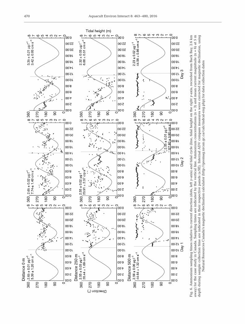
edulis were hung to a depth of 7 m. Mussels were ap-proximately 40−50 mm at the time of sampling andwere hung from the 4 inner circles. The mussel circlewas located on the southeast side of a small salmonfarm, and samples were collected along a linear tran-sect at distances of 0, 250, and 500 m, with a referencelocation at 1500 m (Fig. 4). Sampling was in part op-portunistic, based on vessel availability, weather, andthe availability of analytical personnel. Sub-sampleswere collected for quality assurance of analyticalanalysis. An observation replicate was defined as themean of 2 sub-samples drawn from 1 sampler ‘drop’.Each station and depth (2, 5, and 10 m) was observed3 times, replicated on 3 different days within the sameweek (11, 12, and 15 August 2011), with some excep-tions due to technical difficulties. On Day 1 at the ref-erence site, only 5 m depth samples were collected,and only 2 samples were collected at 5 and 10 m depthfor the 250 m location on Day 2. Total sampling timeon a spe cific day, took approximately 1 h, aiming tocol lect samples during the same tidal cycle, ebb orflood (see Fig. 6). Ammonium concentrations wereanalysed manually using a spectrophotometric tech-nique by Holmes et al. (1999). Current was measuredcontinuously during the 5 d deployment with AcousticDoppler Velocimeters (ADV, Sontek Argonaut) at 5 mdepths at the 0, 250, and 500 m locations, with speedand direction recorded as 5 min averages.

Ammonium results were statistically analysed by1-way ANOVAs to determine differences between locations for each specific depth, and were followed

by 1-tailed t-tests for comparisons of interest (Pal-isade 2014). Where F-tests identified unequal vari-ances, t-tests for unequal variances were applied tocompare means. To determine location means overthe range of conditions during the sampling period,location con centrations were averaged across days(see Fig. 5). Post hoc statistical power tests for 1-wayANOVA and 1-tailed t-tests for independent meanswere estimated with G*power software (Faul et al.2014). The best theoretical distribution was fitted tovelocity data distributions using a parameter estima-tion approach, with best fits ranked by Akaike’sinformation criterion using @RISK software (Palisade2014). Current velocity data were non-normal, andnormality was not achieved after transformation, sonon-parametric Mann-Whitney tests were used toidentify significant differences (p < 0.05) betweenlocations.

Data interpretation

For sampling results on individual days, significantdifferences in ammonium concentrations were iden-tified at each depth, except at 10 m on Days 1 and 2,for which there was insufficient statistical powerfor a credible test (Fig. 5). The largest concentration differences were observed on Day 3 at 5 m depth,when the concentration at the mussel circle was overa third higher than at other locations. Significant concentration differences at locations averaged over

468

Fig. 4. Sampling locations at an integrated multi-trophic aquaculture farm in Canada. An area overview is displayed in the leftpanel; the square indicates the specific study area at high tide (right panel). Dark circle: a blue mussel ‘polar circle’ (70 m circumference); rectangles: kelp rafts; grey circles: Atlantic salmon cages. Sampling locations are denoted with an ‘X’,

with liner distances indicated from 0 m. Latitude and longitude at 0 m are 66.865829°N and 45.029544°E, respectively

Jansen et al.: Design of discrete water sampling programs

the study period (Fig. 5) were identified at 2 and 5 mdepth, but not at 10 m (Table 2). However, only theANOVA at 5 m depth achieved sufficient statisticalpower. The power of the 2 m depth ANOVA was0.75. Upon closer examination, a t-test at 2 m depthbetween the farm concentration and that at 500 m(the location with the smallest concentration dif -ference from the farm) was also significant andachieved sufficient power (0.84) as a 1-tailed test(Table 2), but insufficient power (0.71) as a 2-tailedtest. This suggests slightly different outcomes depend-ing on the test, in which data are partitioned foranalysis, and greater power is achieved if a 1-tailedtest can be used.

Ammonium concentrations at the reference sitewere variable, and reference site measures did not always have the lowest ammonium concentrations ei-ther. On Day 2, for example, reference site concentra-tions were significantly higher than those at the 500and 250 m locations (p < 0.001). If it is assumed thatthe elevated ammonium was from the mussels andthis was generally consistent during and be tweensampling days, the observed concentration differenceswould largely be a function of current flow and tidalcycle during sampling. Current direction at themussel circle (0 m) and at 250 m locations were highlyvariable throughout the entire deployment (Fig. 6).However, samples collected during periods associated

469

Fig. 5. Ammonium depth profiles measured various distances from a mussel circle at an IMTA site in Canada. Samples werecollected on 3 different days over a 5 d summer period (11, 12, and 15 August). Lower right panel: location means averagedover the study period. Error bars are confidence intervals (α = 0.05). Results of 1-way ANOVAs across depths and post hoc sta-tistical power achieved (F-test family) are detailed within respective panels. Statistical insignificance (p > 0.05) and insufficientstatistical power (β – 1 < 0.80) are indicated in bold. Where the ANOVA assumption of homogeneous variances was violated (a,b), t-tests for unequal variances were used to compare the mean farm (0 m) concentration. a: the difference between the farmand the closest concentration value, the reference site, was insignificant (p = 0.90), with insufficient test power (1-tailed = 0.63,2-tailed = 0.45); the difference between the farm and 250 m, the largest concentration difference, was significant (p = 0.03)with sufficient power as a 1-tailed test (1-tailed = 0.90, 2-tailed 0.74); b: the difference between the farm concentration and

250 m, the closed concentration value, was significant (p = 0.019) with sufficient power (1-tailed = 0.99, 2-tailed = 0.95)

Aquacult Environ Interact 8: 463–480, 2016470

Fig

. 6. A

mm

oniu

m s

amp

lin

g t

imes

rel

ativ

e to

cu

rren

t d

irec

tion

(d

ots,

lef

t y-

axis

) an

d t

idal

cyc

le (

lin

e, t

idal

hei

gh

t on

th

e ri

gh

t y-

axis

; rec

ord

ed f

rom

Bac

k B

ay, 2

.6 k

maw

ay)

for

the

case

stu

dy

in C

anad

a. S

amp

lin

g t

imes

are

in

dic

ated

by

the

vert

ical

lin

e. A

mm

oniu

m c

once

ntr

atio

ns

(n =

3)

and

mea

n c

urr

ent

mag

nit

ud

e (n

= 6

) at

5 m

dep

th d

uri

ng

sam

ple

col

lect

ion

tim

e ar

e in

dic

ated

in

th

eir

resp

ecti

ve p

anel

s (±

SE

). I

nte

rnal

AD

V c

omp

ass

mea

sure

s w

ere

corr

ecte

d f

or m

agn

etic

dec

lin

atio

n,

usi

ng

N

atu

ral R

esou

rces

Can

ada’

s m

agn

etic

dec

lin

atio

n c

alcu

lato

r (h

ttp

://g

eom

ag.n

rcan

.gc.

ca/c

alc/

md

cal-

eng

.ph

p)

for

dat

a co

llec

tion

dat

es

Jansen et al.: Design of discrete water sampling programs

with directional change, such as Days 2 and 3, couldbe subject to influence from other farm sources suchas salmon. The high variability of flow direction, evenwithin a particular stage of the tidal cycle, suggestsan absence of a stable near-field ‘nutrient plume’,making it difficult to draw conclusions from samplingprograms based on single sample mean. The samedistribution shapes of current velocity for the 0 and250 m stations (Fig. 7) suggest similar hydrodynamicinfluences at both locations; this seems consistentwith similarities of near-shore locations and the closeproximity to farm structures. The current velocity, di-rection (Fig. 6), and distribution shape (Fig. 7) of the500 m sample suggest an entirely different exposureand current regimen which was more consistent dur-ing stages of the tidal cycles. This is not surprisinggiven the bathymetry of the area, but demonstratesthe difficulty of selecting appropriate reference sitesfor this location.

The slowest average current speed measured overthe 5 d sampling period occurred at the mussel circle,along with the highest mean ammonium concentra-tion in the study (Day 3, 5 m depth). This particularoutcome is consistent with expectations of volumetricloading, dilution, and advection with distance, whereminimal flushing manifests increased nutrient con-centrations; however, this was not always the case.Day 1 and 2 concentrations for this station were simi-lar, despite faster current flow on Day 2. Single con-centration means measured at the mussel circle couldnot consistently be explained by changes in currentflow. This aspect, in combination with the apparent

unreliability of reference con-centrations, make it difficult todetermine the proportionate contribution of ammonium fromaquaculture sources to individualmeasures. Averaged current ve-locities, however, do show a progressive increase (p < 0.05)in mean velocity, moving awayfrom the potential influence offarm structures (Fig. 7).

Conclusions and lessonslearned

A logistically practical sam-pling design of samples collectedon 3 separate days, at 4 differentlocations, and at 3 depths wascapable of identifying a defini-

tive ammonium signal at an IMTA site. Elevated con-centrations at the farm could, in part, be explained byproximity to a mussel circle and current flow dynam-ics. This supports the use of companion parameters,such as current speed and direction in this study, tohelp interpret results of discrete water-quality sam-ples. While higher concentrations were measured atthe farm site, a well-defined gradient measuredacross sampling locations was not readily identifi-ably. This suggests sampling transects should occurcloser to the farm (<250 m), to improve chances ofquantifying a nutrient gradient. Ammonium concen-trations, in general, were variable but relatively mod-est, with the maximum farm concentration approxi-mately a third that of other locations. Variation ofnatural sources is not surprising in light of historicalAugust variation in the embayment—presumably afunction of tidal cycle, other anthropogenic loadingsources, and marine life. All ammonium concentra-tions measured in this study were well within therange of historical values (Martin et al. 2006), sug-gesting that, under the study conditions, ammoniumwas not accumulating in any substantial quantitiesand near-field pelagic impact from the farm was limited.

In the absence of good information on natural vari-ation (a priori data) to guide sampling design, posthoc power tests were a useful tool to determine if suf-ficient statistical power was achieved. Insufficientstatistical power occurred when differences betweenmeans were small or the coefficient of variation (CV;standard deviation/mean) increased, which is consis-

471

Paired n Ammonium SD CV Difference t-test, Power comparison (mean; µmol l−1) (%) from farm p-value achieved

Depth 2 m0 m (farm) 9 2.72 0.32 12.0500 m 9 2.36 0.23 9.9 13.1% 0.030 0.84

Depth 5 m0 m (farm) 9 2.89 0.40 13.7250 m 9 2.46 0.13 5.3 14.6% 0.007 0.90

Depth 10 m0 m (farm) 9 2.70 0.08 2.9Reference 6 2.59 0.12 4.5 3.9% 0.028 0.62

Table 2. Paired comparisons between averaged farm concentrations and the locationwith the smallest difference for the Canadian case study. One-way ANOVAs appliedacross days at each depth, excluding farm means (250 m, 500 m, and the referencesite), showed no significant differences between other location means (2 m depth,p = 0.99; 5 m depth, p = 0.72; 10 m depth, p = 0.87) during the sampling period.t-tests were therefore used to confirm differences only between the farm mean andthe closest concentration value at depth, as listed in the table. The t-tests and posthoc power tests are 1-tailed. Insufficient power in bold. Coefficient of variation

(CV; SD/mean)

Aquacult Environ Interact 8: 463–480, 2016

tent with statistical principles of power analysis(Berndtson 1991). From a scientific perspective,in sufficient power due to small differencesbetween means was less problematic, sincethese concentration differences were ≤0.15 µmoll−1, and arguably negligible, in a biologicalsense. Away from the farm influence, the CV wassmall for individual samples means (i.e. collectedin 1 d), suggesting that sampling duration (timeto collect 3 samples at depth) occurred wellwithin the timeframe for changes of naturalcycles (e.g. tidal). These outcomes may provide acost−benefit rational for reducing sample require -ments at locations where less variation is antici-pated (e.g. reference sites), assuming due con-sideration is given to statistical comparisons withunbalanced data.

CONSIDERATIONS FOR SAMPLING DESIGN,EXECUTION, AND DATA INTERPRETATION

The case studies emphasized several uniquechallenges related to quantification of pelagicinfluences from open-water aquaculture farms.In the following section we further explore sam-pling requirements that should be considered toachieve robust results and to discuss methods toimprove the cost−benefit of sampling regimens.We thereby aim to provide an integral overview(Table 3), including lessons learned from thecase studies, as well as additional informationdrawn from the literature.

Align sampling regimen with study objectives

Defining study objectives is the first step indesigning a sampling scheme. While this seemsrudimentary, different objectives may manifestvery different approaches with regard to theparameters measured, sampling frequency, andspatial or temporal scaling. If for example, theobjective is to quantify the maximal nutrient orparticle signal at a northern temperate water fishfarm, sampling should occur at peak tempera-tures (usually early fall) during second-year pro-duction (Atlantic salmon have an 18−24 mo pro-duction cycle) to ensure biomass, growth rates,feed intake, and, consequently, nutrient loadingare at a maximum (Reid et al. 2013). If the studyobjective is to accurately quantify the effect ofannual nutrient loads, sampling must occur across

472

Fig. 7. Current velocity data distributions at 5 m depths, measuredover 4 d. (a) Mussel circles: (a) 0 m, (b) 250 m, and (c) 500 m. All dis-tributions are non-normal, and significantly different from eachother (p < 0.001). Best theoretical distribution fits for 0 and 250 mlocations are the Pearson 6 distribution, and a general beta distri-

bution, for 500 m location

Jansen et al.: Design of discrete water sampling programs

the range of seasons and biomass values present overa full pro duction cycle. Additional parameters wouldbe re quired if the objective were to identify the bestplacement for co-cultured IMTA species to intercepttransient nutrients. Not only are nutrient concen -trations, current direction, and frequency of changere quired, speed data would also be required, as therate at which organic particles are delivered is just asimportant as the amount (Cranford et al. 2014). Theachievement of ideal study objectives, however, isoften tempered by logistic and analytical realities. Toachieve meaningful results, it should be consideredwhether the maximum practical sampling effort issufficient to achieve the minimally acceptable studyobjectives.

Ambient environmental conditions

Evaluation of the variability of the ambient back-ground conditions is an important consideration forassessing aquaculture effects (Fernandes et al. 2001).Prior (a priori) historical knowledge of abiotic andbiotic conditions at the study site is highly beneficialfor defining sampling requirements. Coastal environ-ments are usually characterized by large natural spa-tial variability. The natural variability of ammoniumconcentrations in the Canadian case study made itdifficult to infer the contribution of farm nutrients tosample means. ‘Baseline analysis’ is also a usefulstrategy to identify starting points for evaluation. Forfish farming this would be represented by the condi-tions prior to farm establishment or when no fish arepresent in pens. This method is sometimes describedas the BACI (Before-After-Control-Impact) design(Stewart-Oaten et al. 1986, Underwood 1991) andhas been used in some studies of ecology and aqua-culture (Rodrí guez-Gallego et al. 2008). Baselinedata can also be used to validate reference stations,as in the Norwegian case study. Reference site(s)provide insight into ambient conditions and variabil-ity, if selected appropriately. Selection of referencesites is non-trivial. Ideally they should be closeenough to the farm to reflect local conditions, but dis-tant enough so as not to be influenced by the farmitself. This is not just an aquaculture research prob-lem; choosing reference sites is an ongoing challengefor all ecological studies (Stewart-Oaten et al. 1986,Smith et al. 1993).

An additional concern with the assessment ofpelagic aquaculture nutrients is that most coastal sys-tems are affected by multiple anthropogenic sources,with the potential to be superimposed over natural

473

Sampling design• Ensure sampling design can meet study objectives, with

due consideration for statistical sample requirements,analytical capacity, and logistical practicalities

• Obtain a priori knowledge of abiotic and biotic condi-tions, if available, to help quantify hydrodynamics and‘patchiness’ of ambient water-quality parameters toguide sampling design

• Exploit high-resolution autonomous or automatedsampling of companion water-quality parameters toassist interpretation of discrete water samples

• Sample in a horizontal transect, orthogonal transect, orgrid surveys where possible, to identify a gradient ofeffects if reference sites are inadequate

• Selection of multiple reference sites will help identifyother sources of spatial variation that could confounddata interpretation

• Define vertical sampling to account for seasonalstratification and depth-dependent data

• Consider requirements for minimal detectable differ-ence between sample means as this will largely dictatethe sample numbers required to achieve acceptablestatistical power—the smaller the difference to bedetected, the larger the sample size required

Sampling execution• Ideally, obtain (planned) information on production,

farm management, and husbandry (i.e. feeding regi-mens, disease treatment, feed delivery, or biofoulingremoval) during the timeframe of sampling to assistwith determining causality of potential effects

• Be aware of vertical water sampler drift to ensuresampling occurs at the intended location

• Consider short-duration sample collection (use ofmultiple vessels could be considered) to reduce con-founding effects of fluctuating tides and currents

• A single ‘drop’ of deployment and sample retrieval froma vertical point sampler should be considered a sample.Multiple water draws from a container should beconsidered sub-samples and not replicate samples

Data analysis & interpretation• Skewed data distributions of water quality at aquacul-

ture sites are not uncommon. Given enough samples,parametric and non-parametric data metrics are apt topresent similar information on data spread (e.g.variation, range). Non-parametric analysis is unlikely toreduce the number of samples required for validstatistical comparison

• Averaging location means across a timeframe of interest(e.g. days, weeks) will help to capture additionalsources of variation

• Irrespective of careful study design and sample collec-tion, conditions at small scales may still vary due toinherent patchiness. A posteriori interpretation oftarget-variable data from discrete sampling, togetherwith companion parameter data, will facilitate datainterpretation to improve robustness of conclusionsdrawn from limited datasets

Table 3. Overview of considerations for sampling design,sampling execution, and data interpretation of discrete

water-quality sampling around aquaculture facilities

Aquacult Environ Interact 8: 463–480, 2016

variability (Fernandes et al. 2001). For cage aquacul-ture studies in developed coastal regions, it may beextremely difficult to find reference sites, remoteenough from other aquaculture operations or otheranthropogenic sources, while still reflective of farm-exposed hydrodynamics (Troell et al. 2003). Wherebaseline data are unavailable, sampling of multiplereference sites can be a powerful assessment tool tohelp ensure ambient spatial variability is captured(Fernandes et al. 2001, Merceron et al. 2002, Reid etal. 2006, Yucel-Gier et al. 2007, Rodríguez-Gallego etal. 2008). However, many studies have only a singlereference location, presumably due to practical con-straints. Sampling along transects may circumventsome of the issues concerning single reference sites,as such sampling can potentially identify concen -tration gradients as a means of inferring causality(discussed in the next section).

The amplitude of ambient nutrient concentrationsmay require special procedural considerations. Typi-cally, the limiting nutrient is of most interest in eval-uating farm-induced effects, i.e. nitrogen in marinesystems (Howarth & Marino 2006) and phosphorus infreshwater (Dillon & Rigler 1974). Both require dif -ferent sampling considerations. Collection of largersample volumes is, for example, advised for ammo-nium measurements in low concentrations (Holmeset al. 1999). Most total phosphorus (TP) techniquesinvolve acid digestion of non-filtered samples (Reidet al. 2006), which means that the presence of par -ticulates may result in higher sample variability or‘spikes’. Sub-samples may then be necessary to identify sources of variation.

Physical processes

Both case studies indicated that hydrographic con-ditions and water exchange mechanisms are keys tounderstanding the distribution of aquaculture dis-charges. The speed at which current passes throughfish cages dictates the volumetric exchange (flushing)and thereby dilution potential (Merceron et al. 2002,Reid & Moccia 2007, Middleton & Doubell 2014).Sampling regimens are often based on site hydrody-namics, and benefit from previous knowledge of cur-rent flows. As shallows or islands can influence localcurrent patterns, impacting current speed and nutri-ent concentrations (Sanderson et al. 2008, Groeskamp& Maas 2012), it is also important to consider the ba-thymetry and hydrography along the chosen transect.

For discrete sampling regimens in coastal eco -systems a horizontal transect is often adopted, with

stations established at a certain distance (e.g. up to1000 m from the cages) down-current from the aqua-culture site (Mantzavrakos et al. 2007, Navarro etal. 2008, Neofitou & Klaoudatos 2008, the presentCanadian case study). Identification of a horizontalgradient—with the appropriate resolution—helps tominimize the confounding effects of variable hydro-dynamics and multiple anthropogenic sources. Otherspatial study designs, for application to complex flowconditions, include orthogonal transects or a grid sur-vey (Fernandes et al. 2001, Sanderson et al. 2008).Spatial gradients obviously provide a greater abilityto assess spatial resolution of nutrient spread thansimple comparisons between farm and referencesites. Furthermore, Sanderson et al. (2008) and Petrellet al. (1993) have reported that inorganic nitrogentransit from fish cages is commonly non-linear; thismay be reflected in the occasionally higher concen-trations measured further from the farm compared tomeasurements directly beside net pens. The authorssuggest this relates to complex near-field hydrody-namics in the proximity of fish cages. As detailed inthe Canadian case study, a range of factors may affectflow patterns, resulting in variable and fluctuatingcurrent directions (Petrell et al. 1993, Huang et al.2008, Reid et al. 2010), consequently leading to com-plex nutrient plume dynamics in the near-fieldor close to structures (Reid & Moccia 2006, 2007).In addition to hydrodynamic influences from cages(Løland 1993, Helsley & Kim 2005, Lader et al. 2007,Le Bris et al. 2007), near-cage currents can be affectedby the swimming behavior of fish (Gansel et al. 2011,2014) as postulated in the Norwegian case study. Thepotential influence to currents and depth of fish ex-cretion and egestion may be important considerations,not only for horizontal vectors, but also for vertical.Waste release is expected to occur at the depth ofmaximum fish biomass, which, in turn, is a function ofenvironmental influences such as temperature andoxygen, as well as feed location and perceived threats(Oppedal et al. 2011), which may vary hourly, diur-nally, and seasonally. Sampling programs that aim toquantify morphology of a ‘nutrient plume’ need to tar-get both vertical and horizontal profiles. At sites withwell-mixed water columns, background values willbe similar across depths (e.g. Fig. 5, Canadian casestudy), whereas in areas with stratified water columns,depth profiles may vary for several variables (e.g.Fig. 2, Norwegian case study). As the latter waterbodies can be partitioned by sharp halo-, thermo-, orpycnoclines, values may change within just a few meters depth. Under such conditions, sampling depthmay strongly affect environmental parameters.

474

Jansen et al.: Design of discrete water sampling programs

Sample collection mechanics (sampling execu-tion) should therefore be considered, especially inrelation to the effects of flow velocity and depth. Current and drag forces can induce swing ofthe deployment line holding the water sampler,with swing magnitude potentially increasing withdepth. This may result in sampling bias, with thegreatest potential for deviation along the horizontalaxis. The authors have routinely observed draginducing a swing of between 5° and 15°. If forexample, a sample is collected at a 10 m depthwith a drag-induced swing of 15° on the deploy-ment line, the Pythagorean theorem indicates ahorizontal displacement of 2.6 m and a verticaldeviation of 0.35 m. While this may not seemmuch, some near-field data requirements such asthe placement of co-cultured species in IMTA maynecessitate spatial data on the scale of severalmeters. Displacement becomes more problematic ifsuch accuracy is re quired at greater depths. If thedepth is increased to 30 m, the same angle ofswing causes a horizontal displacement of 7.8 mand a vertical deviation of 1 m.

Apart from the effects of physical processes onhorizontal and vertical spatial variability, temporalaspects should not be neglected given that, intidally driven areas, water column properties canchange within hours. If a study aims to quantifywater-quality data under relatively consistent envi-ronmental conditions, sampling should occur withinthe duration of a specific tidal phase, to improve thechances of capturing such conditions. This presentsa very short sampling window. However, samplingwithin a specific tidal phase is no guarantee of con-sistent predictable flow either (see Norwegian casestudy), and unpredictable and unstable flow direc-tions might be observed near and around farmstructures (see Canadian case study). Appropriatedata integration across time, at each location, willhelp to quantify temporal variation and should ulti-mately reveal the magnitude of effects spatially (seeCanadian case study). The resultant location meanwill be a combined function of the effect magni-tude and occurrence frequency. When comparingbetween seasons, or sampling during a stormy sea-son, one should be aware of the resuspension ofbottom material or breaking down of pycnoclines.Resuspension of material requires a certain thresh-old level of energy; once such thresholds arereached by extreme events, nutrient conditions canchange and affect water-column properties sig -nificantly, especially for shallow sites (Wallin &Håkanson 1991, Jones et al. 2012).

Farm management and husbandry

Waste released from commercial farms is not a con-tinuous process but varies on temporal scales and, inaddition to environmental factors, can be influencedby farm husbandry practices. Short-term (diurnal anddaily) variation in waste release may be influenced byfeeding regimens (Lander et al. 2013) and variableammonia release with post-prandial excretion peaks(Brett & Zala 1975), while phosphorus can leach im-mediately from aquafeeds upon submersion in water(Reid & Moccia 2006). Occasional disease and treat-ment may result in a reduction or cessation of feeding(Ashley 2007). Furthermore, the cleaning of nets to remove biofouling adds a recurring waste flux fromfarms. Sampling should be avoided during such epi -sodic events. Long-term variation in nutrient loadingis also a function of the farm production cycle. Fishbiomass increases until harvest, and, in the case of Atlantic salmon in temperate waters, almost 4 timesmore nutrients will be released in the second yearof production (Reid et al. 2013). The stage of the production cycle therefore strongly influences theamount of feed entering the water, consumption,and nutrient loading accordingly. Variation in farm husbandry practices, such as changes in feeding regi-men, fish harvesting, off-feed events (e.g. veterinarytreatment), and site fallowing may influence pelagicsampling strategies and the interpretation of results. Itis therefore beneficial to obtain knowledge about thefarm site, husbandry practices, and production details,if available, before devising an appropriate samplingstrategy.

Statistical considerations

The data analysis approach is primarily a functionof study objectives, and there are many good re -sources detailing experimental design and analysis(e.g. Quinn & Keough 2002). We therefore only high-light some of the most relevant considerations to thestatistical analysis of discrete water samples.

The ‘patchiness’ and variability of nutrient concen-trations around fish cages may result in skewed datadistributions. This is often a result of a few elevatedmeasures in combination with a fixed minimumvalue, such as the background concentration, whichmay result in a non-normal distribution (Reid et al.2006). As there will be no measures below the back-ground concentration, the lower end of the data distri-bution may be abrupt, and the asymptotic tail whichoccurs in a normal distribution, absent. It may there-

475

Aquacult Environ Interact 8: 463–480, 2016

fore be tempting to consider non-parametric statisticalapproaches in these circumstances. However, non-parametric statistics are not as good at detecting dif-ferences among means (Steel et al. 1997) and maytherefore require more samples in order to achievesufficient power for detecting differences comparedto parametric approaches. This suggests that the useof non-parametric statistical tests does not resolve issues of large sample requirements. As the numberof sample ‘replicates’ increases, error measures ofmeans (parametric) and medians (non-parametric)from the same samples will eventually overlap andcommunicate similar information (Reid et al. 2006).

The collection of true replicates for discrete watersampling is an important consideration. Multiplewater draws from a single sampler ‘drop’ are, inessence, sub-samples and are likely to reflect theanalytical technique rather than the variation in timeand space at the sampling location. Treating these astrue replicates is apt to underestimate the actual vari-ation. This means that collection of statistical repli-cates necessitates multiple sampler ‘drops’. How-ever, as a result of dynamic water movement aroundaquaculture facilities, deploying multiple ‘drops’actually leads to sampling of different pockets ofwater. Therefore, this approach does not necessarily

result in the collection of true sample replicateseither, but samples can be considered spatial repli-cates during the time of collection.

The number of sample replicates required toachieve the desired statistical power is an importantconsideration for experimental design or the post hocassessment of the power achieved. For discrete con-centrations in the Canadian case study, it was theprobability of correctly rejecting a null hypothesis ofammonium concentrations being equal, when theyare not. Table 4 shows the replicates per treatmentgroup for a priori power testing, for the 2-tailed tests(p < 0.05) needed to achieve a power of 80%, whichis the minimum statistical power recommended forpara metric tests (Berndtson 1991). As the percent dif-ference that is detected between samples decreasesor the treatment coefficient of variation (CV) in -creases, the replicates needed increase expo -nentially. Therefore, careful consideration of studyobjectives, such as the minimum effect size requiringdetection, is needed, as this could substantially affectthe number of replicates required. In the absence ofdetailed a priori variation data, post hoc power testsare a useful tool in determining whether sufficientstatistical power has been achieved. Results from theCanadian case study suggest how increasing spatialand temporal sample coverage can affect samplenumbers. Under a similar CV and detectable differ-ence be tween means (>0.15 µmol l−1), a sample size(n) of 9 was just sufficient to achieve acceptable sta-tistical power for 1-tailed tests of independent means(see also Table 2 and Fig. 5). Under similar conditionsof 9 replicates per location, a modest sampling regi-men of 4 loca tions at 3 different depths necessitates108 samples. This suggests that a thorough spatialcoverage of aquaculture sites with discrete samplecollection, necessitating wet chemistry techniques,can quickly become logistically and analyticallyexpensive. Large sample numbers will also requirelonger collection times, increasing the chance thatenvironmental conditions may change during collec-tion. In the Norwegian case study, current directionchanged from 60° to 160° within 30 min, emphasizingthe need for rapid sampling to document instanta-neous conditions (i.e. ‘snap-shot’).

Companion parameters

Given the limitations to discrete sampling and,therefore, the limited number of samples, companionparameter data can help to interpret discrete sampleresults or can help to design a robust sampling pro-

476

CV Difference from reference to be detected (%)(%) 5 10 15 20 25 30 35 40 45 50

1 3 22 4 3 23 7 3 3 24 12 4 3 3 25 17 6 4 3 3 26 24 7 4 3 3 3 27 32 9 5 4 3 3 3 28 42 12 6 4 3 3 3 3 29 52 14 7 5 4 3 3 3 3 210 63 17 9 6 4 4 3 3 3 312 91 24 12 7 5 4 4 3 3 314 124 32 15 9 7 5 4 4 3 316 161 42 19 12 8 6 5 4 4 318 204 52 24 14 10 7 6 5 4 420 252 63 29 17 12 9 7 6 5 425 393 99 45 26 17 12 10 8 6 630 566 142 63 37 24 17 13 10 9 735 770 193 86 50 32 23 17 14 11 940 1005 252 112 63 42 29 22 17 14 1245 1272 318 142 80 52 37 27 21 17 1450 1571 393 175 99 63 45 34 26 21 17

Table 4. Replicates needed per treatment group for studiesof 80% power at p < 0.05, for 2-tailed tests with 2-treatmentexperiments (modified from Berndtson 1991). For experi-ments with a 1-tailed test, the replication shown would provide an experiment of 90% power at p < 0.025. Coeffi-

cient of variation (CV; SD/mean)

Jansen et al.: Design of discrete water sampling programs

gram. Ideally, good current flow data obtained dur-ing the sampling campaign can indicate whetherwater flowing from cages is being directed to near-field sampling locations. Fine-scale hydrodynamicmodelling of plume dynamics can provide the con-text for fieldwork site selection and sampling design.But there are also valuable alternative approaches.One option is the application of discrete sampling incombination with other continuously measured indi-cators, such as dissolved oxygen, temperature, pH,salinity, and turbidity. Continuous sampling using insitu sensors enables greater sampling frequency and,therefore, better measures of variation. ContinuousCTD measures in the Norwegian case study (Fig. 2)showed that water column characteristics were dif-ferent between farming and reference stations, sug-gesting that higher particle abundance was not nec-essarily a function of the farm and that results fromdiscrete samples should be interpreted with care.Reid et al. (2006) demonstrated that a strong inverserelationship between total phosphorus and dissolvedoxygen occurred directly in trout cages, a lesser rela-tionship down-current, and no relationship up-cur-rent from the cages. The magnitude of the variationand the strength of the relationship (r2) reflected cur-rent direction and dilution with distance, relative tofish location. The oxygen−phosphorus relationshipsuggests that continuously measured companionpara meters collected in situ at fish cages could beused as proxies for nutrient concentration trends.

The development of in situ sensors in aquatic sci-ences is in its infancy but is evolving rapidly, for com-panion parameters as well as for variables of interest(Bende-Michl & Hairsine 2010, Mukhopadhyay &Mason 2013, Wild-Allen & Rayner 2014). At present,in situ electronic monitoring technology can enableeither sufficient temporal coverage or good spatialcoverage, but often not both simultaneously. Multi-probes or CTDs (i.e. conductivity, temperature, anddissolved oxygen) work well for temporal assess-ment, but when deployed autonomously they aretypically left in 1 location over days or weeks. Con -tinuously monitoring submersible instruments thatare boat towed (Brager et al. 2015) or autonomousremote operating vehicles, can enable good spatialcoverage, but these are typically limited to collectiondurations on the order of hours. Ironically, there mayalso be challenges with large amounts of data. Evenshort sampling episodes using sensors can producelarge amounts of data compared to discrete sampleresults. Such large data volumes may require varioustools for post-processing, and issues like auto-corre-lation may become relevant.

Another useful proxy for nutrient dispersal is theuse of bioindicators. In aquaculture studies, biomark-ers such as stable isotopes, fatty acid profiles, andpigments are progressively being used to trace fishwastes in seaweeds (Garcia-Sanz et al. 2010) andshellfish (Mazzola & Sara 2001, Both et al. 2012,Graydon et al. 2012, Handå et al. 2012b, Jiang et al.2013). In order to identify a signal from biomarkers,the needed timeframe of applicability may be onthe order of months to years. An alternative time-integrated approach suited to shorter timeframes,such as days to months, is the use of biocollectors orsediment traps. Biocollectors are substrates that canbe used to sample commonly occurring fouling or -ganisms and are similar in design to those used formonitoring aquatic invasive species (Sephton et al.2011). With the rationale being that, with the provi-sion of appropriate habitat and all things being ofequal density, fouling would increase as a functionof nutrient availability. The merits of this approachare under investigation in an aquaculture context(Cooper 2013). Sediment traps can also be deployedto collect settling material (Findlay & Watling 1997),although this is typically done to assess benthic im -pacts. Slow-settling particulate wastes are oftendiluted to an extent that limits detection in discretewater samples; sedimentation over a timeframe ofdays to weeks may provide greater discriminativepower when comparing locations (authors’ unpubl.data).

Considerations of biological activity, far-field, andcumulative effects

Upon consideration of pelagic sampling design, itshould be acknowledged that dispersion of farmwastes is not solely a function of hydrodynamics, asconcentrations of dissolved particulate and inorganicnutrients are also a function of fish nutrient load,background concentrations, as well as ambient bio-logical activity. The uptake and transformation offarm waste products can be very rapid, especially innutrient-limited systems, and may become manifestas reduced farm nutrient concentrations in the watercolumn. Overall environmental impact should there-fore be evaluated according to both the living andnon-living suspended fractions in the water column(Sará 2007c).

Discrete sampling programs often target the local-ized footprint of a farm, usually as a function of studyobjectives, but intensive fish farming may also affectregional impacts on marine ecosystems. Hence, envi-

477

Aquacult Environ Interact 8: 463–480, 2016

ronmentally sustainable fin-fish farming necessitatesan understanding of the farming impact potentialbeyond the immediate production area (Husa et al.2014). There is, however, a knowledge gap on wastespread and persistence over large areas, as well as onthe cumulative effects of multiple farms in a region(Price et al. 2015). Far-field or regional effects gener-ally require different tools, such as biomarkers (seealso ‘Companion parameters’ above) or modelling(Skogen et al. 2009). Near-field nutrient plumes canbe modelled assuming an appropriate distance fromcages, choosing a reasonable timeframe for sampleintegration (e.g. a daily average), and making theappropriate simplifying assumptions (Reid & Moccia2007, Middleton & Doubell 2014). As an extension ofthis approach, models with volumetric loading andspatial components can subsequently be scaled up todetermine the assimilative capacity of a region(Strain & Hargrave 2005, Skogen et al. 2009; see alsoECASA toolbox at http://www.ecasatoolbox. org. uk/the-toolbox/informative/matrix-files/fin-fish-farming-environmental-impact-assessment). In regions wherethere are multiple potential loading sources withinthe same body of water, the possibility of synergisticeffects could also be considered through modelling(Fernandes et al. 2001). Models do not negate theneed for data collection, but require data for modeldevelopment and validation, and, consequently,appropriately designed sample regimens.

CONCLUSIONS

With this paper we demonstrated that discretepelagic sample collection within a dynamic systemlike commercial-scale aquaculture sites presents aunique set of challenges. Adequately capturing thespatial and temporal dynamics often requires largesample numbers, which may lead to practical andlogistical limitations in discrete sampling regimens.Consideration of the balance between the informa-tion needed and the effort expended to acquire itis, therefore, non-trivial. Assuming study limitationshave been properly identified and applying thestrategies discussed in this paper (summarized inTable 3), the amount of information from discretesample data sets can be maximized. When the needdoes arise for discrete sample collection of pelagicnutrients, farm operators and researchers need notbe discouraged once armed with the appropriate tools.

Acknowledgements. This work was supported by grant no.216201 (EXPLOIT) awarded by the Norwegian Research

Council, and the Natural Sciences and EngineeringResearch Council of Canada (NSERC) strategic CanadianIntegrated Multi-Trophic Aquaculture Network (CIMTAN).The Institute of Marine Research facilitated sample collec-tion for the Norwegian case study by proving research ves-sel time, and we thank the crew of R/V ‘Brattstrøm’ for theirassistance and Marine Harvest A/S for providing access tothe farming locations. Data collection for the Canadian casestudy would not have been possible without Fisheries andOceans Canada, the Canadian Coast Guard crew of the SARvessel ‘Viola M. Davidson’ and our industry partner, CookeAquaculture Inc. We thank Peter Cranford and anonymousreviewers for constructive remarks on earlier versions of themanuscript, and thanks to Bill Brendtson for granting per-mission to publish Table 4 which is based on Brendtson(1991).

LITERATURE CITED

Arai R, Akita K, Nishiyama T, Nakatani N, Otsuka K,Nishiyama T (2011) Measuring instrument for dissolvedinorganic nitrogen and phosphate ions. Int J OffshorePolar Eng 21: 44−49

Ashley PJ (2007) Fish welfare: current issues in aquaculture.Appl Anim Behav Sci 104: 199−235

Bende-Michl U, Hairsine PB (2010) A systematic approachto choosing an automated nutrient analyser for rivermonitoring. J Environ Monit 12: 127−134

Berndtson WE (1991) A simple, rapid and reliable methodfor selecting or assessing the number of replicates foranimal experiments. J Anim Sci 69: 67−76

Borja Á, Rodríguez JG, Black K, Bodoy A and others (2009)Assessing the suitability of a range of benthic indices inthe evaluation of environmental impact of fin and shell-fish aquaculture located in sites across Europe. Aqua -culture 293: 231−240

Both A, Parrish CC, Penney RW (2012) Growth and bio-chemical composition of Mytilus edulis when reared oneffluent from a cod, Gadus morhua, aquaculture facility.J Shellfish Res 31: 79−85

Boyd D, Wilson M, Howell T (2001) Recommendations foroperational water quality monitoring at cage aqua cultureoperations. Environmental monitoring and reportingbranch, Ontario Ministry of the Environment, Toronto

Brager LM, Cranford PJ, Grant J, Robinson SMC (2015) Spa-tial distribution of suspended particulate wastes at open-water Atlantic salmon and sablefish aquaculture farmsin Canada. Aquacult Environ Interact 6: 135−149

Brager LM, Cranford PJ, Jansen H, Strand Ø (2016) Tempo-ral variations in suspended particulate waste concentra-tions at open-water fish farms in Canada and Norway.Aquacult Environ Interact 8:437–452

Brett JR, Zala CA (1975) Daily pattern of nitrogen excretionand oxygen consumption of sockeye salmon (Onco -rhynchus nerka) under controlled conditions. J Fish ResBoard Can 32: 2479−2486

Brooks KM, Stierns AR, Mahnken CVW, Blackburn DB(2003) Chemical and biological remediation of the benthos near Atlantic salmon farms. Aquaculture 219: 355−377

Chopin T, Cooper JA, Reid G, Cross S, Moore C (2012)Open-water integrated multi-trophic aquaculture: envi-ronmental biomitigation and economic diversification offed aquaculture by extractive aquaculture. Rev Aquacult4: 209−220

Cooper JA (2013) Quantifying energy and nutrient dispersal

478

Jansen et al.: Design of discrete water sampling programs

and scales of influence on wild species from open-waterIMTA sites. In: Martell DJ, Duhaime J, Parsons GJ (eds)Canadian aquaculture R&D review 2013. AquacultureAssociation of Canada, Ottawa, p 55

Cranford PJ, Duarte P, Robinson SMC, Fernández-ReirizMJ, Labarta U (2014) Suspended particulate matterdepletion and flow modification inside mussel (Mytilusgalloprovincialis) culture rafts in the Ría de Betanzos,Spain. J Exp Mar Biol Ecol 452: 70−81

Dillon PJ, Rigler FH (1974) The phosphorus−chlorophyllrelationship in lakes. Limnol Oceanogr 19: 767−773

Faul F, Buchner A, Erdfelder E, Lang AG (2014) G*Power.University of Düsseldorf, Düsseldorf

Fernandes TF, Eleftheriou A, Ackefors H, Eleftheriou M andothers (2001) The scientific principles underlying themonitoring of the environmental impacts of aquaculture.J Appl Ichthyol 17: 181−193

Findlay RH, Watling L (1997) Prediction of benthic impactfor salmon net-pens based on the balance of benthic oxy-gen supply and demand. Mar Ecol Prog Ser 155: 147−157

Gansel LC, Rackebrandt S, Oppedal F, McClimans TA(2011) Flow fields inside stocked fish cages and the nearenvironment. Proc Int Conf Ocean Offshore Arctic Eng30:201−209

Gansel LC, McClimans TA, Myrhaug D (2012) Flow aroundthe free bottom of fish cages in a uniform flow with andwithout fouling. J Offshore Mech Arctic Eng 134:011501

Gansel L, Rackebrandt S, Oppedal F, McClimans TA (2014)Flow fields inside stocked fish cages and the near envi-ronment. J Offshore Mech Arctic Eng 136: 201−209

Gao QF, Cheung KL, Cheung SG, Shin PKS (2005) Effects ofnutrient enrichment derived from fish farming activitieson macroinvertebrate assemblages in a subtropicalregion of Hong Kong. Mar Pollut Bull 51: 994−1002

Garcia-Sanz T, Ruiz-Fernandez JM, Ruiz M, Garcia R, Gon-zalez MN, Perez M (2010) An evaluation of a macroalgalbioassay tool for assessing the spatial extent of nutrientrelease from offshore fish farms. Mar Environ Res 70: 189−200

Graydon CM, Robinson SMC, Scheibling RE, Cooper JA(2012) Canthaxanthin as a potential tracer of salmon feedin mussels (Mytilus spp.) and sea urchins (Strongylo -centrotus droebachiensis). Aquaculture 366−367: 90−97

Groeskamp S, Maas LRM (2012) Ship-borne contour inte-gration for flux determination. J Sea Res 74: 26−34

Handå A, Min H, Wang X, Broch OJ, Reitan KI, ReinertsenH, Olsen Y (2012a) Incorporation of fish feed and growthof blue mussels (Mytilus edulis) in close proximity tosalmon (Salmo salar) aquaculture: implications for inte-grated multi-trophic aquaculture in Norwegian coastalwaters. Aquaculture 356−357: 328−341

Handå A, Ranheim A, Olsen AJ, Altin D, Reitan KI, Olsen Y,Reinertsen H (2012b) Incorporation of salmon fish feedand feces components in mussels (Mytilus edulis): impli-cations for integrated multi-trophic aquaculture in cool-temperate North Atlantic waters. Aquaculture 370−371: 40−53

Harendza A, Visscher J, Gansel L, Pettersen B (2008) PIV oninclined cylinder shaped fish cages in a current and theresulting flow field. American Society of MechanicalEngineers, New York, NY, p 555−563

Helsley CE, Kim JW (2005) Mixing downstream of a sub-merged fish cage: a numerical study. IEEE J Oceanic Eng30: 12−19

Holmer M, Hansen PK, Karakassis I, Borg JA, Schembri PJ(2008) Monitoring of environmental impacts of marineaquaculture. In: Holmer M, Black K, Duarte CM, Marbà

N, Karakassis I (eds) Aquaculture in the ecosystem.Springer, Heidelberg, p 47–85

Holmes RM, Aminot A, Kerouel R, Hooker BA, Peterson BJ(1999) A simple and precise method for measuringammonium in marine and freshwater ecosystems. Can JFish Aquat Sci 56: 1801−1808

Howarth RW, Marino R (2006) Nitrogen as the limiting nutri-ent for eutrophication in coastal marine ecosystems: evolving views over three decades. Limnol Oceanogr 51: 364−376

Huang CC, Tang HJ, Liu JY (2008) Effects of waves and cur-rents on gravity-type cages in the open sea. AquacultEng 38: 105−116

Hudson JJ, Taylor WD, Schindler DW (1999) Planktonicnutrient regeneration and cycling efficiency in temper-ate lakes. Nature 400: 659−661

Husa V, Kutti T, Ervik A, Sjøtun K, Hansen PK, Aure J (2014)Regional impact from fin-fish farming in an intensiveproduction area (Hardangerfjord, Norway). Mar Biol Res10: 241−252

Jiang ZJ, Wang GH, Fang JG, Mao YZ (2013) Growth andfood sources of Pacific oyster Crassostrea gigas inte-grated culture with sea bass Lateolabrax japonicus inAilian Bay, China. Aquacult Int 21: 45−52

Jones EM, Kämpf J, Fernandes M (2012) Characterisation ofthe wave field and associated risk of sediment resuspen-sion in a coastal aquaculture zone. Ocean Coast Manage69: 16−26

Karakassis I, Tsapakis M, Hatziyanni E, Papadopoulou KN,Plaiti W (2000) Impact of cage farming of fish on theseabed in three Mediterranean coastal areas. ICES J MarSci 57: 1462−1471

Kutti T, Ervik A, Hansen PK (2007) Effects of organic efflu-ents from a salmon farm on a fjord system. I. Verticalexport and dispersal processes. Aquaculture 262: 367−381

Lader PF, Olsen A, Jensen A, Sveen JK, Fredheim A, Ener-haug B (2007) Experimental investigation of the interac-tion between waves and net structures—damping mech-anism. Aquacult Eng 37: 100−114

Lander TR, Robinson SMC, MacDonald BA, Martin JD(2013) Characterization of the suspended organic parti-cles released from salmon farms and their potential as afood supply for the suspension feeder, Mytilus edulis inintegrated multi-trophic aquaculture (IMTA) systems.Aquaculture 406–407: 160−171

Le Bris H, Dhaouadi R, Naviner M, Giraud E and others(2007) Experimental approach on the selection and per-sistence of anti-microbial-resistant aeromonads in faecalmatter of rainbow trout during and after an oxolinic acidtreatment. Aquaculture 273: 416−422

Løland G (1993) Water-flow through and around net pens.In: Reinertsen H, Dahle LA, Jørgensen L, Tvinnereim K(eds) Fish farming technology. Proc 1st Int Conf Fish FarTech. Balkema, Rotterdam, p 177−183

Macleod CK, Crawford CM, Moltschaniwskyj NA (2004)Assessment of long term change in sediment conditionafter organic enrichment: defining recovery. Mar PollutBull 49: 79−88

Mantzavrakos E, Kornaros M, Lyberatos G, Kaspiris P (2007)Impacts of a marine fish farm in Argolikos Gulf (Greece)on the water column and the sediment. Proc Environ SciTech Symp 9:110−124

Martin JL, LeGresley MM, Strain PM (2006) Plankton moni-toring in the Western Isle Region of the Bay of Fundyduring 1999−2000. Can Tech Rep Fish Aquat Sci 2629

Mazzola A, Sara G (2001) The effect of fish farming organicwaste on food availability for bivalve molluscs (Gaeta

479

Aquacult Environ Interact 8: 463–480, 2016

Gulf, Central Tyrrhenian, MED): stable carbon isotopicanalysis. Aquaculture 192: 361−379

Merceron M, Kempf M, Bentley D, Gaffet JD, Le Grand J,Lamort-Datin L (2002) Environmental impact of asalmonid farm on a well flushed marine site. I. Currentand water quality. J Appl Ichthyol 18: 40−50

Middleton JF, Doubell M (2014) Carrying capacity for finfishaquaculture. Part I—Near-field semi-analytic solutions.Aquacult Eng 62: 54−65

Mukhopadhyay SC, Mason A (2013) Smart sensors for real-time water quality monitoring. Springer, Heidelberg

Navarro N, Leakey RJG, Black KD (2008) Effect of salmoncage aquaculture on the pelagic environment of temper-ate coastal waters: seasonal changes in nutrients andmicrobial community. Mar Ecol Prog Ser 361: 47−58

Neofitou N, Klaoudatos S (2008) Effect of fish farming on thewater column nutrient concentration in a semi-enclosedgulf of the eastern Mediterranean. Aquacult Res 39: 482−490

Oppedal F, Dempster T, Stien LH (2011) Environmentaldrivers of Atlantic salmon behaviour in sea-cages. RevAquacult 311: 1−18

Palisade (2014) @RISK for Excel. Palisade Corporation,Ithaca, NY

Petrell R, Tabrizi K, Harrison P, Druehl L (1993) Mathemati-cal model of Laminaria production near a BritishColumbian salmon sea cage farm. J Appl Phycol 5: 1−14

Price C, Black KD, Hargrave BT, Morris JA Jr (2015) Marinecage culture and the environment: effects on water qual-ity and primary production. Aquacult Environ Interact 6: 151−174

Quinn GP, Keough MJ (2002) Experimental design anddata analysis for biologists. Cambridge University Press,Cambridge

Reid GK, Moccia RD (2006) Diel fluctuation of soluble phos-phorus in the tank water of rainbow trout, Oncorhynchusmykiss (Walbaum), and relationships with feed inputsand dissolved oxygen. Aquac Res 15: 1606−1610

Reid GK, Moccia RD (2007) Estimating aquatic phosphorusconcentrations 30 metres down-current from a rainbowtrout cage array. J Environ Monit 9: 814−821

Reid GK, McMillan I, Moccia RD (2006) Near-field loadingdynamics of total phosphorus and short-term water quality variations at a rainbow trout cage farm in LakeHuron. J Environ Monit 8: 947−954

Reid GK, Liutkus M, Bennett A, Robinson SMC, MacDonaldB, Page F (2010) Absorption efficiency of blue mussels(Mytilus edulis and M. trossulus) feeding on Atlanticsalmon (Salmo salar) feed and fecal particulates: implica-tions for integrated multi-trophic aquaculture. Aqua -culture 299: 165−169

Reid GK, Chopin T, Robinson SMC, Azevedo P, Quinton M,Belyea E (2013) Weight ratios of the kelps, Alaria escu-lenta and Saccharina latissima, required to sequester dissolved inorganic nutrients and supply oxygen forAtlantic salmon, Salmo salar, in Integrated Multi-TrophicAquaculture systems. Aquaculture 408/409: 34−46

Rodríguez-Gallego L, Meerhoff E, Poersch L, Aubriot L,Fagetti C, Vitancurt J, Conde D (2008) Establishing limitsto aquaculture in a protected coastal lagoon: impact ofFarfantepenaeus paulensis pens on water quality, sedi-ment and benthic biota. Aquaculture 277: 30−38

Sætre R (2007) The Norwegian coastal current—oceano -graphy and climate. Tapir Academic Press, Trondheim

Sanderson JC, Cromey CJ, Dring MJ, Kelly MS (2008) Dis-tribution of nutrients for seaweed cultivation aroundsalmon cages at farm sites in north-west Scotland. Aqua-culture 278: 60−68

Sará G (2007a) Aquaculture effects on some physical andchemical properties of the water column: a meta-analysis.Chem Ecol 23: 251−262

Sará G (2007b) Ecological effects of aquaculture on livingand non-living suspended fractions of the water column: a meta-analysis. Water Res 41: 3187−3200

Sará G (2007c) A meta-analysis on the ecological effects ofaquaculture on the water column: dissolved nutrients.Mar Environ Res 63: 390−408

Sephton D, Vercaemer B, Nicolas JM, Keays J (2011) Moni-toring for invasive tunicates in Nova Scotia, Canada(2006−2009). Aquat Invasions 6: 391−403

Skogen MD, Eknes M, Asplin LC, Sandvik AD (2009) Mod-elling the environmental effects of fish farming in a Nor-wegian fjord. Aquaculture 298: 70−75

Smith EP, Orvos DR, Cairns J Jr (1993) Impact assessmentusing the Before-After-Control-Impact (BACI) model: concerns and comments. Can J Fish Aquat Sci 50: 627−637

Steel RGD, Torrie JH, Dickey DA (1997) Principles and pro-cedures of statistics: a biometrical approach. McGraw-Hill, New York, NY

Stewart-Oaten A, Murdoch WW, Parker KR (1986) Environ-mental impact assessment: ‘Pseudoreplication’ in time?Ecology 67: 929−940

Strain PM, Hargrave BT (2005) Salmon aquaculture, nutri-ent fluxes and ecosystem processes in southwestern NewBrunswick. In: Hargrave BT (ed) Environmental effectsof marine finfish aquaculture. Springer, Heidelberg,p 29−57

Troell M, Halling C, Neori A, Chopin T, Buschmann AH,Kautsky N, Yarish C (2003) Integrated mariculture: ask-ing the right questions. Aquaculture 226: 69−90

Underwood A (1991) Beyond BACI: experimental designsfor detecting human environmental impacts on temporalvariations in natural populations. Mar Freshw Res 42: 569−587

Valdemarsen T, Bannister RJ, Hansen PK, Holmer M, ErvikA (2012) Biogeochemical malfunctioning in sedimentsbeneath a deep-water fish farm. Environ Pollut 170: 15−25

Wallin M, Håkanson L (1991) Nutrient loading modelsfor estimating the environmental effects of marine fishfarms. In: Mäkinen T (ed) Marine aquaculture and envi-ronment. Nordic Council of Ministers, Copenhagen

Wild-Allen K, Rayner M (2014) Continuous nutrient obser-vations capture fine-scale estuarine variability simulatedby a 3D biogeochemical model. Mar Chem 167: 135−149

Wilson A, Magill S, Black K (2009) Review of environmentalimpact assessment and monitoring in salmon aquacul-ture In: Environmental impact assessment and monitor-ing in aquaculture. Fish Aquacult Tech Pap 527, FAO,Rome, p 455−535

Yucel-Gier G, Kucuksezgin F, Kocak F (2007) Effects of fishfarming on nutrients and benthic community structure inthe eastern Aegean (Turkey). Aquacult Res 38: 256−267

480

Editorial responsibility: Adam Hughes, Oban, UK

Submitted: February 10, 2016; Accepted: July 6, 2016Proofs received from author(s): August 11, 2016

➤

➤

➤

➤

➤

➤

➤

➤

➤

➤

➤

➤

➤

➤

➤

➤

➤

➤

➤

➤

➤

➤

➤

➤

➤