Eurographics Symposium on Geometry Processing (2005)M. Desbrun, H. Pottmann (Editors)

Discrete Willmore Flow

Alexander I. Bobenko1 and Peter Schröder2

1TU Berlin 2Caltech

AbstractThe Willmore energy of a surface,

∫(H2 −K)dA, as a function of mean and Gaussian curvature, captures the

deviation of a surface from (local) sphericity. As such this energy and its associated gradient flow play an impor-tant role in digital geometry processing, geometric modeling, and physical simulation. In this paper we considera discrete Willmore energy and its flow. In contrast to traditional approaches it is not based on a finite ele-ment discretization, but rather on an ab initio discrete formulation which preserves the Möbius symmetries ofthe underlying continuous theory in the discrete setting. We derive the relevant gradient expressions including alinearization (approximation of the Hessian), which are required for non-linear numerical solvers. As exampleswe demonstrate the utility of our approach for surface restoration, n-sided hole filling, and non-shrinking surfacesmoothing.

Categories and Subject Descriptors (according to ACM CCS): G.1.8 [Numerical Analysis]: Partial Differential Equa-tions; I.3.5 [Computer Graphics]: Computational Geometry and Object Modeling; I.6.8 [Simulation and Model-ing]: Types of Simulation.

Keywords: Geometric Flow; Discrete Differential Geometry; Willmore Energy; Variational Surface Modeling;Digital Geometry Processing.

1. Introduction

The Willmore energy of a surface S ⊂ R3 is given as

EW (S) =∫

S(H2−K)dA = 1/4

∫S(κ1−κ2)2 dA,

where κ1 and κ2 denote the principal curvatures, H =1/2(κ1 + κ2) and K = κ1κ2 the mean and Gaussian curva-ture respectively, and dA the surface area element. Immer-sions of surfaces which minimize this energy are of greatinterest in several areas:

• Theory of surfaces: the Willmore energy of a surfaceis conformally invariant [Bla29] making it an importantfunctional in the study of conformal geometry [Wil00];

• Geometric modeling: for compact surfaces with fixedboundary a minimizer of EW (S) is also a minimizerof total curvature

∫S κ1

2 + κ22 dA which is a stan-

dard functional in variationally optimal surface model-ing [LP88, WW94, Gre94];

• Physical modeling: thin flexible structures are governed

by a surface energy of the form

E(S) =∫

Sα +β (H−H0)2− γK dA,

the so-called Canham-Helfrich model [Can70, Hel73](H0 denotes the “spontaneous” curvaturewhich plays an important role in thin-shells [GKS02, BMF03, GHDS03]). For α = H0 = 0,β = γ the Canham-Helfrich model reduces to theWillmore energy.

In all of these application areas one typically deals with theassociated geometric flow

S =−∇E(S),

(time derivatives are denoted by an overdot) which drivesthe surface to a minimum of the potential energy given byE(S). In the theory of surfaces as well as in geometric mod-eling one is interested in critical points of E(S). In physicalmodeling the solution shape is characterized by a balance ofexternal and internal forces. In this setting the internal forcesare a function of the Willmore gradient.

c© The Eurographics Association 2005.

A.I. Bobenko & P. Schröder / Discrete Willmore Flow

Contributions In this paper we explore a novel, discreteWillmore energy [Bob05] and introduce the associated geo-metric flow for piecewise linear, simplicial, 2-manifoldmeshes. In contrast to earlier approaches the discrete flowis not defined through assemblies of lower level discrete op-erators, nor does the numerical treatment employ operatorsplitting approaches. Instead the discrete Willmore energy,defined as a function of the vertices of a triangle mesh, isused directly in a non-linear numerical solver to affect theassociated flow as well as solve the static problem. Since thediscrete formulation has the same symmetries as the continu-ous problem, i.e., it is Möbius invariant, the associated prop-erties, such as invariance under scaling, carry over exactlyto the discrete setting of meshes. To deal effectively withboundaries we introduce appropriate boundary conditions.These include position and tangency constraints as well asa free boundary condition. We demonstrate the method withsome examples from digital geometry processing and geo-metric modeling.

1.1. Related Work

We distinguish here between discrete geometric flows, i.e.,flows based on discrete analogues of continuous differentialgeometry quantities, and those based on discretizations ofcontinuous systems. The guiding principle in the construc-tion of the former is the preservation of symmetries of theoriginal continuous system, while the latter is based on tra-ditional finite element or finite difference approaches whichin general do not preserve the underlying symmetries. Thereis also a broad body of literature which uses linearized ver-sions of the typically non-linear geometric functionals. Suchapproaches are not based on intrinsic geometric properties(e.g., replacing curvatures with second derivatives) but ratherdepend on the particular parameterization chosen. For thisreason we will not further consider them here.

Discrete Flows In the context of mesh based geometricmodeling a number of discrete flows have been consid-ered. For example, Desbrun et al. [DMSB99] used meancurvature flow (α = 1, β = γ = H0 = 0) to achieve de-noising of geometry. Pinkall and Polthier [PP93] used arelated approach, area minimizing flow, to construct dis-crete minimal surfaces. Critical points of the area functionalalso play an important role in the construction of discreteharmonic functions [DCDS97], their use in parameteriza-tions [EDD∗95, DMA02], and the construction of confor-mal structures for discrete surfaces [Mer01, GY03]. Sincethe underlying “membrane” energy is second order only, itcannot accomodate G1 continuity conditions at the bound-ary of the domain. These are important in geometric mod-eling for the construction of tangent plane continuous sur-faces. Fourth order flows on the other hand can accomo-date position and tangency conditions at the boundary. Per-haps the simplest fourth order flow is surface diffusion, i.e.,flow by the Laplace-Beltrami operator of mean curvature,S = −∆SH. Such discrete flows were studied by Schneider

and Kobbelt [SK01], Xu et al. [XPB05], and Yoshizawa andBelyaev [YB02]. In each case the approach was based ontaking the square of a discrete Laplace-Beltrami operatorcombined with additional simplifications to ease implemen-tation. Unfortunately surface diffusion flow can lead to sin-gularities in finite time [MS00] leading to “pinching off” ofsurfaces which are too thin. Yoshizawa and Belyaev [YB02]demonstrate this behavior and show the comparison withWillmore flow, which leads to much better results in this re-gard. This difference in behavior between surface diffusionand Willmore flows is due to the additional terms appearingin the Euler-Lagrange (EL) equation of the Willmore flow

∆SH +2H(H2−K) = 0.

Yoshizawa and Belyaev took the EL equation as their start-ing point and defined a discrete Willmore flow by assem-blying the components from individual, well known discreteoperators. Unfortunately in that discrete setting propertiessuch as H2−K ≥ 0 can no longer be guaranteed. In contrastwe define our discrete Willmore energy directly using theMöbius invariance of the integrand (H2−K)dA as the fun-damental principle. Among other properties one achieves theH2−K ≥ 0 always, as expected (see Section 2).

Discretized Flows Both surface diffusion and Willmoreflows have been treated numerically through a variety of dis-cretizations. For example, Tasdizen et al. [TWBO03] andChopp and Sethian [CS99] use a level set formulation forsurface diffusion flow, while Mayer [May01] uses finite dif-ferences, and Deckelnick et al. [DDE03] use finite elements.For Willmore flow finite element approaches were pursuedby Hari et al. [HGR01] and Clarenz et al. [CDD∗04]. A levelset formulation was given by Droske and Rumpf [DR04]. Inthese approaches no attempt is made to preserve the Möbiussymmetries. On the other hand they do have the advantagethat a rich body of literature applies when it comes to er-ror and convergence analysis. Our approach as of now lacksa complete analysis of this type. Partial results on the con-vergence of the discrete Willmore energy to the continuousWillmore energy are discussed at the end of Section 2.

2. Discrete Willmore Energy

In this section we recall the definition of the discrete Will-more energy and some of its relevant properties.

The derivation of the discrete Willmore energy is based onthe observation that the integrand

(H2−K)dA

is invariant under Möbius transformations [Bla29], i.e.,translations, rotations, uniform scale, and inversion. The firsttwo are obvious and the latter two follow from the changeof variable formula [Che73]. This immediately implies thatEW (S) itself is a conformal invariant of the surface. Note thatfor compact closed surfaces we also have EH(S) =

∫S H2 dA

as a conformal invariant [Whi73]. However the integrand of

c© The Eurographics Association 2005.

A.I. Bobenko & P. Schröder / Discrete Willmore Flow

EH(S) is not Möbius invariant. It is for this reason that weprefer EW over EH (the latter is used by some authors as thedefinition of the Willmore energy).

The Möbius invariance is a natural mathematical discretiza-tion principle. The importance of this property depends onthe particular application one is interested in. For the nu-merical construction of Willmore surfaces, which are criti-cal points (in particular minima) of the Willmore energy, itis essential. For applications such as smoothing and denois-ing of meshes (see Section 4) a concrete benefit is the scaleinvariance of the Willmore energy.

We are interested in evaluating this energy for discrete sur-faces, i.e., surfaces given as topological 2-manifold config-urations of simplicies. Such a “mesh” consists of verticesvi = (xi,yi,zi)T (i = 1, . . . ,N) and the topological complex isgiven as a set of edges ei j connecting vi with v j and trian-gles ti jl bounded by vertices vi, v j and vl and edges ei j, e jl ,and eli (see Figure 1). For notational simplicity we assumethat the surface is closed (i.e., each edge ei j is bounded byexactly two triangles, ti jl and t jik) and that triangles incidenton a given edge are consistently oriented (note however thatwe do not assume global orientability). Boundaries will bediscussed in Section 3.3.

vkt jik

ti jl

a

d

e

b

c

vl

vi

v j

Figure 1: Notation for vertices, edges and triangles in thevicinity of a given edge e = (vi,v j) = ei j; a = ek j, b = e jl ,c = eli, d = eik.

The discrete Willmore energy on a mesh is defined at eachvertex vi as

Wi = ∑ei j

βij −2π,

i.e., a sum over the edges incident to vi of certain angles β ij,

which measure the angle between the circumcircles definedby the two triangles ti jl and t jik incident to the given edgeei j (see Figure 2). Obviously Wi is Möbius invariant since itsdefinition is based on angles between circles. The Willmoreenergy of the entire mesh is then simply the sum, W = ∑i Wi.For later use we also recall the definition of discrete Gausscurvature at a vertex vi

Ki = 2π−∑tik j

αik j.

Here α ik j denotes the Euclidean angle at i inside the triangle

tik j.

β ij

vk

v j

vl

vi

Figure 2: Geometry of β ij.

The geometric picture is as follows. A given edge has two in-cident triangles. Each triangle has a circumcircle. Since thefour vertices forming the two triangles are (generically) on acommon sphere (possibly at infinity) the two circumcirclesare also on this sphere. The two circles meet in the verticesvi and v j where they intersect. Consider a tangent vector toeach circle at vi. These two tangent vectors make the angleβ i

j which lies in the tangent plane to the sphere at that point.

Note that this geometric setup implies that β ij = β

ji . Suppose

now vi and all its neighbors v j (i.e., corresponding to edgesei j) lie on a common sphere and that the (embedded) 1-ringof vi is convex. In that case it is easy to see that the β i

j neatlyadd up to exactly 2π in the tangent plane at vi and henceWi = 0 (see Figure 3) as expected. Now suppose that vi andits neighboring vertices do not share a common sphere. Inthat case Wi > 0. To see this use the Möbius invariance of theenergy and map the central point vi to infinity by a Möbiustransformation. All circles passing through vi are mappedto straight lines and the energy becomes the sum ∑ j β i

j ofthe external angles of a non-planar closed polygon in threespace. In that interpretation the inequality ∑ j β i

j ≥ 2π fol-lows easily [Bob05] (this inequality is a polygonal version ofFenchel’s theorem [Fen29, Spi75]). With the same argumentone also concludes that Wi +Ki ≥ 0, i.e., ∑ j β i

j−∑k j α ik j ≥ 0,

reflecting the fact that H2 dA is always non-negative.

Finally we observe that Wi ≥ 0 and that it vanishes iff vi andall its edge neighbors v j lie on a common sphere and the ver-tex vi is convex. These two conditions are equivalent to thecondition that the triangles meeting at vi build a Delaunaytriangulation on a sphere.

Smooth Limit The discrete Willmore energy W is not onlyan analogue of the continuous one. It approximates the con-tinuous Willmore energy W in a “natural” limit. Let (u,v) 7→f (u,v) be a curvature line parameterization of a surface.Without loss of generality consider the vicinity of the ori-gin (u,v) = (0,0) in the tangent plane where we have

(u,v) 7→ (u,v,12(κ1u2 +κ2v2)+o(u2 + v2)),

with κ1,κ2 denoting the principal curvatures of the sur-face at the point (0,0). Now consider a triangular latticeLε = {ε(la + mb + nc) : l,m,n ∈ Z} in the parameter planegenerated by three vectors a,b,c with a+b+c = 0. Here ε isa small parameter. Consider the hexagon Dε in the parameter

c© The Eurographics Association 2005.

A.I. Bobenko & P. Schröder / Discrete Willmore Flow

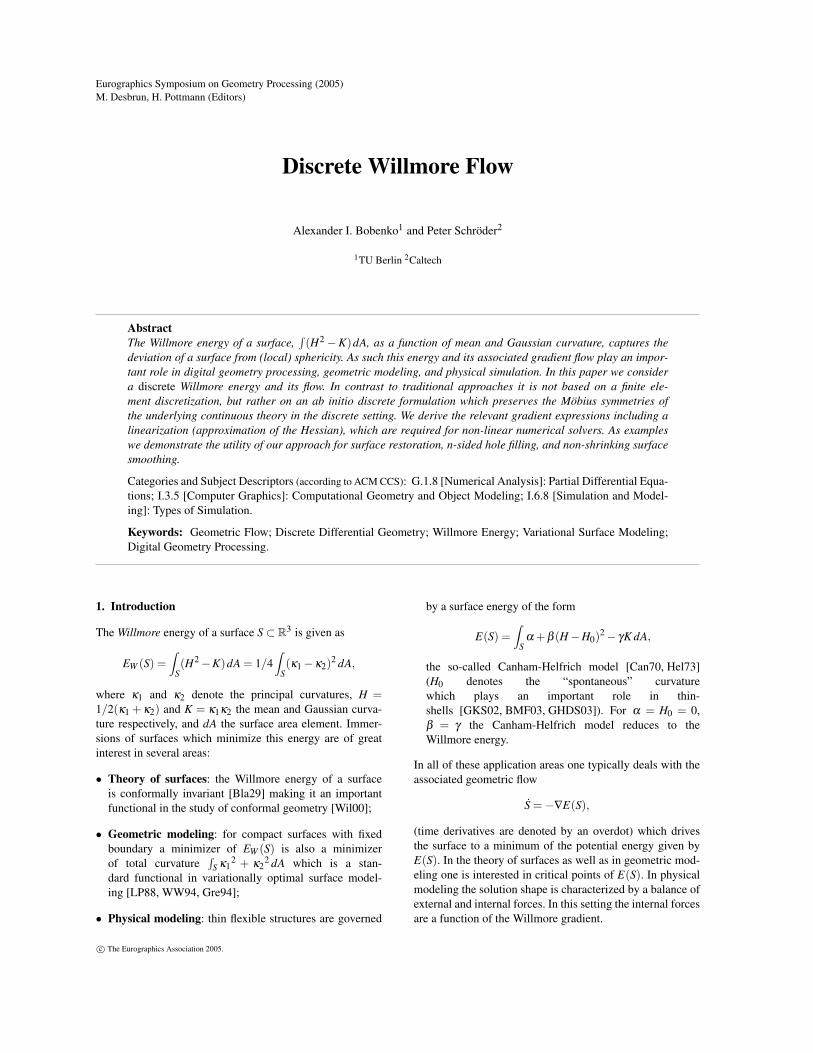
Figure 3: Geometry of ∑ei jβ i

j around a vertex. The an-gles between subsequent circumcircles—appropriate tan-gent vectors are indicated with colors corresponding to thecircumcircles of each triangle—neatly add up to 2π if allvertices are co-spherical.plane with vertices p1 = εa, p2 =−εc, p3 = εb, p4 =−εa,p5 = εc, p6 = −εb and its image f (Dε ) on the surface.Let W (Dε ) be the smooth Willmore energy of f (Dε ). Onthe other hand, the vertices f (pi), i = 1, . . . ,6 together withf (0) build a simplicial surface with six triangles. Denote byW (Dε ) the discrete Willmore energy of this surface and con-sider the quotient of the discrete and smooth Willmore ener-gies of such an infinitesimal hexagon

R = limε→0

W (Dε )W (Dε )

.

A direct but rather complicated computation leads to the fol-lowing conclusions:

1. R is independent of the curvatures κ1,κ2,

2. R≥ 1, and R = 1 iff the lattice Lε has two of its directionsaligned with the curvature lines of the surface (two of thevectors a,b,c are curvature line directions).

Thus, after sufficiently many 1 → 4 refinements of thesmooth surface the discrete Willmore energy approximatesthe smooth one if the curvature line net is triangulated, oth-erwise the discrete energy is larger.

The question whether the discrete Willmore energy can beused as a variational method for computation of curvatureline nets is currently under investigation (see also Figures 8and 9).

3. Evaluation

For the numerical treatment of discrete Willmore flow andthe solution of energy minimization problems we need ef-fective evaluation procedures for the Willmore energy andits derivatives. To simplify the implementation of these func-tions we begin with a discussion of the definition of the an-gles β i

j and some of the consequent symmetries in the ex-pressions.

3.1. Definition of Intersection Angles

Consider edge ei j and its two incident triangles t jik and ti jlwith associated vertices vk, v j, vl , and vi (see Figure 1).Defining the four directed edge vectors

A = a|a| = v j−vk

|v j−vk | B = b|b| = vl−v j

|vl−v j |

C = c|c| = vi−vl

|vi−vl | D = d|d| = vk−vi

|vk−vi|

the angles follow as

cosβij = −R(Q) =−R(AB−1CD−1)

= 〈A,C〉〈B,D〉−〈A,B〉〈C,D〉−〈B,C〉〈D,A〉,

where 〈., .〉 denotes the usual Euclidean dot product andR(Q) the real part of the normalized cross ratio of the fouredges bounding the “diamond” formed by the two trian-gles incident on edge ei j. This cross ratio is defined interms of quaternion algebra with the standard identifica-tion of 3-vectors with imaginary quaternions, R3 ≡ I(H),v 7→ (0, ix, jy,kz)T (i2 = j2 = k2 =−1, i j = k, jk = i, ki = j).The subsequent expression of this quaternion cross ratio interms of Euclidean inner products follows from the rules ofquaternion multiplication and Lagrange’s identity for the in-ner product between two cross products. More details can befound in [Bob05].

Properties of β ij and its Derivatives A number of surpris-

ing facts—which we exploit to significantly simplify the ex-pressions needed by the numerical solver—are immediatelyobvious from the above definition. To clarify these we makeall arguments explicit, β i

j = β (k, j, l, i) going around the di-amond in counter clockwise order. We already noted earlierthat β (k, j, l, i) = β (l, i,k, j). In fact from the formula forcosβ (k, j, l, i) it terms of scalar products it is immediatelyclear that β (k, j, l, i) is invariant under all cyclic permuta-tions and reflections of its arguments. In particular if we flipthe edge ei j 7→ ekl the cosine of the angle remains the same.

From the invariance under cyclic and reflection permutationsof its arguments it also follows that all first derivatives canbe written as a single function f1(., ., ., .) with suitably per-muted arguments

β,k = f1(k, j, l, i) β, j = f1( j, l, i,k)

β,l = f1(l, i,k, j) β,i = f1(i,k, j, l).

(Here and in what follows we use comma notation to denotepartial derivatives with respect to the corresponding argu-ment and write β := β i

j to reduce clutter.)

3.2. Energy Gradient

For gradient flow numerical computations we require thegradient of the discrete Willmore energy. A direct calcula-

c© The Eurographics Association 2005.

A.I. Bobenko & P. Schröder / Discrete Willmore Flow

tion readily yields

−sin(β )β,k = (− 1|a|

PA(C)〈B,D〉+ 〈A,C〉 1|d|

PD(B)

+1|a|

PA(B)〈C,D〉−〈A,B〉 1|d|

PD(C)

−〈B,C〉( 1|d|

PD(A)− 1|a|

PA(D))).

Here we used PX = I−X⊗X as shorthand for the projectionoperator into the orthogonal complement of (the unit vector)X .

Remarkably, if we separate out the linear dependence of thisexpression on a, b, c, and d we arrive at a scalar linear com-bination

− sin(β )β,k = (cosβ

|a|2− 〈B,C〉|a||d|

)a

+(〈A,C〉|b||d|

+〈C,D〉|b||a|

)b

−(〈A,B〉|c||d|

+〈B,D〉|c||a|

)c

−(cosβ

|d|2− 〈B,C〉|a||d|

)d. (1)

In a semi-implicit time stepping algorithm this amounts torequiring only the solution of a sparse linear system of sizen×n rather than (3n)× (3n) for n vertices, a very attractivefeature. In fact Equation 1 can serve as a linearized versionof the Hessian of the energy. See Section 4 for further com-ments on this fact.

For the free boundary treatment we also need expressionsfor the gradient of the angle between two edges. Desbrunand co-workers [DMA02] (Appendix B) derive these and wewill not repeat them here.

Gradient Singularity If vk, v j, vl , and vi are co-circular thenβ = 0 and β,k is not defined. For vertices in general posi-tions this does not occur. However, in practice the case thatthe four vertices of a diamond are nearly co-circular, whilerare, does occur. For some inputs it can in fact be a frequentoccurance (see for example Figure 12). Consider a quadran-gulation of a smooth surface which is turned into a trianglemesh through insertion of diagonals in each quad. In thissetting the diagonal edges very often have β nearly equal tozero.

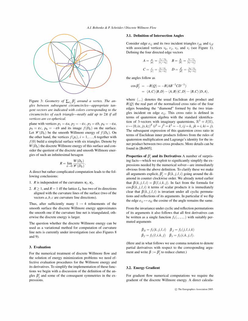
Keeping in mind that in the end we care about the directionof negative gradient, i.e., steepest descent, of the discreteWillmore energy we make the following geometric obser-vation. In case β = 0 there is one direction of varying vk inwhich the angle does not change (infinitesimally). This is thetangential direction to the circle C passing through the pointsvi,v j,vk and vl . For (infinitesimal) unit motions in all or-thogonal directions the angle β increases at equal rate. Thisproperty of the gradient is conformal and thus preserved un-der Möbius transformations. It can be seen more easily in a

Möbius transformed picture. Send the point vi to infinity bythe inversion in a sphere centered at vi. Both circles in Fig-ure 4 become straight lines. Let v j, vk, vl be the images of thevertices v j,vk,vl under this Möbius transformation. For thecase of β = 0 both circles in Figure 4 are coincident—callthis common circle C—and the points v j, vk and vl becomecollinear: they lie on the straight line L which is the Möbiusimage of the circle C. The only direction of varying vk inwhich the angle does not change is along the straight line L.Variations in all orthogonal directions increase the angle atequal rate.

vk

v j

vl

vi

vk

v j

vlβ

Figure 4: After sending vi to infinity, the two circles havebeen mapped to two lines which intersect with angle β .

Consider now a given vertex vi and assume for the momentthat only one β contributing to the gradient computationat vi vanishes. Let C 3 vi be the corresponding circle withfour vertices lying on it. Let all other, well defined, negativegradient directions sum to g. Decompose a variation direc-tion G = Go + Gp of vi into the parts orthogonal Go ⊥ Cand parallel Gp ‖C to the tangent of the circle in vi and letg = go + gp be the same decomposition of g. The contribu-tion to the gradient from all “regular” (non-vanishing) β ’s is−〈g,G〉 and the contribution of the vanishing β is R | Go |with some R > 0. For the whole gradient this implies

−Gpgp +(| Go | R−〈Go,go〉).

Thus the total negative gradient direction, i.e. the directionin which the energy decreases the most is gp (parallel to C)if R >| go | and gp +go(1−R/ | go |) if R <| go |.

The case of multiple β ’s in the support of the gradient of Wiwith respect to the given vertex vi vanishing, is more com-plicated. One can get the negative gradient direction (if it ex-ists) in this case from the following non-linear minimizationprocess. To each of the edges en with vanishing β (en) = 0there corresponds a circle Cn through vi. For the variationG the contribution to the gradient of this edge is | Rn ×G |where Rn is a vector tangent to Cn. We define

δ = min|G|=1,〈G,g〉≥0

∑n|Rn×G|− 〈G,g〉

where the sum is taken over all vanishing β from the 1-ringwith flaps of vi. The first term measures the length of the pro-jection of G into the orthogonal complement of Rn, i.e., theamount of (infinitesimal) increase of energy while the sec-ond term measures the decrease in energy for the directionG. If δ > 0 no motion exists which decreases the energy and

c© The Eurographics Association 2005.

A.I. Bobenko & P. Schröder / Discrete Willmore Flow

the direction of steepest descent is the zero vector. If δ < 0the direction G which achieves the minimum is our soughtafter steepest descent direction with magnitude |δ |.

The case that all β in the support of the gradient of vi vanishsimultaneously, corresponds to a configuration which putsall vertices in the 1-ring with flaps of vi including vi itselfonto a common circle. In this case no direction decreasingthe Willmore energy at vi exists.

In our implementation we have experimented with the non-linear minimization to find a valid direction of energy de-crease (or zero if none exists) but found it to give the sameresults (numerically) as a far simpler heuristic: if |sinβ |< ε

set the corresponding gradient to zero. We found ε = 10−6

to give reliable results in double precision for all our experi-ments.

3.3. Boundary Conditions

So far we have implemented two types of boundary condi-tions.

G1-boundary The variational problem we are dealing withis a fourth order system. To be well posed it requires twoindependent boundary conditions. The most natural choicehere is to fix positions and normals at a boundary. We spec-ify this kind of boundary data on a mesh by fixing posi-tions of the boundary vertices and those vertices within oneedge distance from the boundary. The normals of the tri-angles of this boundary strip can be treated as normals onthe boundary. This boundary condition fits perfectly for G1-gluing of surfaces. Typical applications are surface restora-tion and smooth filling of a hole (see Figures 10 and 11).Note that the method requires no conditions on the topol-ogy of the mesh. In particular one can fix some “islands” ofinternal vertices (or faces) of the required surface.

Free Boundary Alternatively we have experimented withclosing boundary curves by adding a vertex at infinity toeach boundary loop. This is an unusual treatment since it ac-tually removes the boundary and adds a Dirichlet conditionat infinity. The idea comes from Möbius geometry where theinfinity point is not distinguished.

e

β2(e)

vb

β3(vb)

e

Figure 5: Free boundary conditions. Boundary edges e ande, and a boundary vertex vb with the angles β2 and β3.

For simplicity consider a surface with one boundary curve.

By adding the infinity point and connecting it to each bound-ary vertex we obtain a closed surface. We distinguish threetypes of edges of this surface E = Ei ∪ Eb ∪ E∞: internaledges Ei, boundary edges Eb of the original surface and newedges E∞ incident to the infinity point. The circumcirclespassing through the infinity point are straight lines. The dis-crete Willmore energy of the closed surface consists of threeterms

∑e∈E

β (e) = ∑e∈Ei

β1(e)+ ∑e∈Eb

β2(e)+ ∑e∈E∞

β3(e).

The first term is just the discrete Willmore energy of the orig-inal surface. The angles β2(e) are associated to the bound-ary edges e ∈ Eb and are the intersection angles of theseedges with the circumcircles of the corresponding bound-ary triangles. Another interpretation for β2(e) is that this isπ minus the angle of the boundary triangle opposite to theedge e ∈ Eb. Finally the angle β3(e) is associated to the ad-ditional edge e ∈ E∞ connecting ∞ to a boundary vertex vb.Equivalently it can be associated to the boundary vertex vb.This is the intersection angle of two circumcircles (which arestraight lines in this case) passing through vb and ∞, i.e., theintersection angle of two boundary edges meeting at vb (seeFigure 5).

The resulting behavior is that of a free boundary (see Fig-ure 7; right column).

4. Numerical ExperimentsWe have implemented the discrete Willmore gradient flowusing linear and non-linear solvers from the excellentPETSc [BBE∗04] and TAO [BMMS04] libraries, allowingus to experiment with a wide variety of pre-canned solvers,while needing to supply only the gradient, respectively theapproximation of the Hessian (Equation 1). For the timediscretization we experimented with both the forward andbackward Euler method. For the forward Euler method thetime step limitation imposed by the Courant condition forfourth order problems—time increments must be of the or-der of the fourth power of the shortest edge in the mesh—is too severe to be practical except for very simple meshes.The backward Euler method leads to a non-linear problemat each step. These can be solved with a full Newton methodrequiring evaluation of the Hessian of the energy at each iter-ation step. We did derive the expressions for the Hessian, butfound that the effort was not justified as a function of eval-uation cost and numerical behavior. The latter was no betterin our experiments than a much simpler approach based ona semi-implicit time discretization using the linearized ver-sion of the gradient (Equation 1). In that setup only a linearsystem must be solved at each time step to find the positionincrement ∆x(t)

(1dt

I+K(t))∆x(t) =−∇E(t).

Here dt is the time step and a super script (t) denotes quan-tities evaluated at time t. The matrix K is n× n where n is

c© The Eurographics Association 2005.

A.I. Bobenko & P. Schröder / Discrete Willmore Flow

the number of (free) vertices and collects the terms of Equa-tion 1. Assuming an average valence of six, each row of thematrix contains (on average) thirteen non-zero entries (1-ring with flaps plus the center vertex). The full Hessian hasnon-trivial 3×3 blocks instead and results in a linear systemof size (3n)× (3n).

The use of such approximations is well established andworks well in practice though the usual convergence guar-antees of Newton methods are missing. Desbrun and co-workers [DMSB99] used a similar approach when they per-formed implicit mean curvature flow with a constant ma-trix per time step. Recall that the coefficients of the “cotanformula” change throughout the time step. Keeping themconstant corresponds to a similar linearization of the gra-dient as we employed. For the particular case of problemsinvolving squared curvature bending energies Hauth andco-workers [HES03], similarly found that inexact Newtonmethods using even fairly aggressive linearizations of gradi-ents work very well.

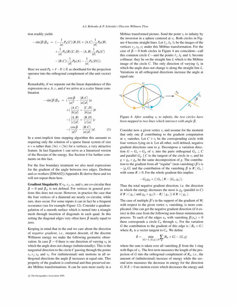
Figures 6 and 7 show some simple examples. The icosahe-dron is subdivided linearly four times and becomes essen-tially a perfect sphere within a few minimization steps (Fig-ure 6). After 24 steps convergence was achieved with a finalenergy of 10−7 (a perfect sphere would be zero). The dif-ference between fixed and free boundary conditions is illus-trated with the cathead example (Figure 7). First the resultof flow with fixed boundaries then the result of keeping theboundaries free (both intermediate and final state shown).The latter evolves to a planar polygon with convex bound-aries. In the latter example we show the circumcircles for alltriangles.

Figure 8 shows the evolution of a torus. The initial meshis a coarse torus linearly subdivided twice. Almost immedi-ately the vertices flow to the surface of a geometric torus.Subsequent evolution aligns edges with the principal curva-ture directions (and “fattens” the torus). The edge alignmentalso becomes apparent in the flat-shaded highlights. Figure 9shows a pipe with two boundary loops which are circular (inessence half the torus example with fixed boundaries). Thesame evolution as with the torus can be observed with thelong term behavior evolving towards a “fat” pipe.

Figure 10 shows a standard benchmark example from k-sided (six in this case) hole filling. An initial triangulationwith boundaries coming from a Loop subdivision surface isrelaxed under the Willmore flow. With the two outermost“rows” of vertices fixed tangent continuity across the bound-ary is assured. Note that this example starts in a configura-tion with many edges having β = 0. Our simple strategy ofsetting these gradients to zero works quite well in this exam-ple. After a few steps all β angles have become sufficientlynon-zero (above our threshold of ε = 10−6) that the flowproceeds as expected.

Figure 11 shows an example of mesh restoration. A set oftriangles is marked as free while all others are held fixed.

Figure 6: Subdivided icosahedron rapidly evolves to asphere.

Figure 7: Cathead evolved with fixed boundaries (left col-umn) and free boundaries (right column). In each case theoriginal mesh is followed by an intermediate state of the evo-lution and the final state.

The free vertices flow to “repair” the scar with a surface sec-tion which smoothly (G1) interpolates the surrounding fixedsurface (compare to the example in [CDD∗04]).

Finally Figure 12 shows an example of geometry denois-ing. The mesh smoothed in this case is the raw result of alight field scanner with typically small amplitude noise dueto measurement error. In particular for examples of this typethe non-shrinking nature of the Willmore flow (the energy isscale invariant) favors it over standard approaches based onmean curvature flow. The mesh contains over 37k vertices(and 88 boundary loops). This mesh is particularly chal-lenging since it contains many edges with β near zero: theoriginal mesh is a triangulated quadrangulation. It also hasmany triangles with very high aspect ratio right next to small,round triangles. Figure 12 shows the original mesh followedby the results of 10 respectively 100 smoothing steps.

c© The Eurographics Association 2005.

A.I. Bobenko & P. Schröder / Discrete Willmore Flow

Figure 8: A twice linearly subdivided torus mesh evolvesquickly towards a geometric torus with long term flowchanging the shapes of triangles so as to align edges withprincipal curvature directions.

Figure 9: Time evolution of a pipe with circular boundaryconditions. Compare with Figure 8.

5. Conclusion

In this paper we have considered a discrete Willmore flow.The discrete energy is expressed in terms of circles and theangles they make with one another and therefore Möbiusinvariant, reproducing the symmetries of the continous en-ergy. The discrete energy approaches the continuous energyin the infinitesimal limit for regular triangulations with twoedges aligned with principal curvature directions. We haveexperimented with a number of different linear and non-linear solvers and found a simple linear approximation ofthe Hessian to be sufficient in our experiments.

Ongoing investigations are geared towards more powerfulnumerical methods. Especially for large meshes a multi-grid solver for the linear systems arising in the semi-implicittime stepping method may well provide significant speedupsover our current (unoptimized) implementation. Possible fu-ture directions include the use of Willmore gradient flow forthe construction of variational subdivision schemes whichwould optimize functionals such as

∫κ1

2 +κ22 dA in a fully

non-linear fashion. Another interesting avenue is the useof the Willmore functional to construct curvature line nets.We have observed that the discrete Willmore flow leads to

Figure 10: Smooth filling of a six sided hole. On the upperleft the original configuration showing the underlying mesh.The boundary triangles follow a smooth outline and fix po-sition and tangency constraints (all other vertices are un-constrained). Evolution to the energy minimum is illustratedthrough a number of intermediate steps with the final holefill in the lower right. All shaded images use triangle nor-mals for shading without interpolation.

Figure 11: Surface restoration for the Egea model. A regionto be restored is outlined (top). All vertices in the blue trian-gles are unconstrained with the surrounding vertices provid-ing position and tangency constraints. Results of the energyminimization (before and after; bottom).

c© The Eurographics Association 2005.

A.I. Bobenko & P. Schröder / Discrete Willmore Flow

Figure 12: Denoising of scanned geometry. On the left theoriginal mesh with noise due to an active light stripe basedscanner. Followed by the results of 10 and 100 smoothingsteps (37k vertices; 88 boundary loops).meshes aligned with the curvature lines of the surface. Thisphenomenon, theoretically partially explained in Section 2,is quite natural since the curvature lines are also a subject ofMöbius geometry. A closely related problem, currently un-der investigation, is the definition of the discrete Willmoreenergy for quadrilateral meshes, which in a sense would bemore natural for curvature line nets.

Acknowledgments This work was supported in part by NSF(DMS-0220905, DMS-0138458, ACI-0219979), DFG (Re-search Group “Polyhedral Surfaces” and Research CenterMATHEON “Mathematics for Key Technologies” Berlin),DOE (W-7405-ENG-48/B341492), nVidia, the Center forIntegrated Multiscale Modeling and Simulation, Alias, andPixar. Special thanks to Kevin Bauer, Oscar Bruno, MathieuDesbrun, Ilja Friedel, Cici Koenig, Nathan Litke, and FabioRossi.

References

[BBE∗04] BALAY S., BUSCHELMAN K., EIJKHOUT

V., GROPP W. D., KAUSHIK D., KNEPLEY M. G.,MCINNES L. C., SMITH B. F., ZHANG H.: PETScUsers Manual. Tech. Rep. ANL-95/11 - Revision 2.1.5,Mathematics and Computer Science Division, ArgonneNational Laboratory, 2004. Available at http://www-unix.mcs.anl.gov/petsc/petsc-2/. 6

[Bla29] BLASCHKE W.: Vorlesungen über Differentialge-ometrie III. Springer, 1929. 1, 2

[BMF03] BRIDSON R., MARINO S., FEDKIW R.: Sim-ulation of clothing with folds and wrinkles. In Proceed-ings of the 2003 ACM SIGGRAPH/Eurographics Sympo-sium on Computer animation (2003), Eurographics Asso-ciation, pp. 28–36. 1

[BMMS04] BENSON S. J., MCINNES L. C., MORÉ J.,SARICH J.: TAO User Manual (Revision 1.7). Tech. Rep.ANL/MCS-TM-242, Mathematics and Computer Science

Division, Argonne National Laboratory, 2004. Availableat http://www-unix.mcs.anl.gov/tao. 6

[Bob05] BOBENKO A. I.: A Conformal Energy for Sim-plicial Surfaces. In Combinatorial and ComputationalGeometry, Goodman J. E., Pach J.„ Welzl E., (Eds.),MSRI Publications. Cambridge University Press, 2005,pp. 133–143. 2, 3, 4

[Can70] CANHAM P. B.: The Minimum Energy of Bend-ing as a Possible Explanation of the Biconcave Shape ofthe Human Red Blood Cell. Journal of Theoretical Biol-ogy 26 (1970), 61–81. 1

[CDD∗04] CLARENZ U., DIEWALD U., DZIUK G.,RUMPF M., RUSU R.: A Finite Element Method forSurface Restoration with Smooth Boundary Conditions.Computer Aided Geometric Design 21, 5 (2004), 427–445. 2, 7

[Che73] CHEN B.-Y.: An Invariant of Conformal Map-pings. Proceedings of the American Mathematical Society40, 2 (1973), 563–564. 2

[CS99] CHOPP D. L., SETHIAN J. A.: Motion by Intrin-sic Laplacian of Curvature. Interfaces and Free Bound-aries 1, 1 (1999), 107–123. 2

[DCDS97] DUCHAMP T., CERTAIN A., DEROSE T.,STUETZLE W.: Hierarchical Computation of PL Har-monic Embeddings. Tech. rep., University of Washington,1997. 2

[DDE03] DECKELNICK K., DZUIK G., ELLIOTT C. M.:Fully Discrete Semi-Implicit Second order Splitting forAnisotropic Surface Diffusion of Graphs. SIAM J. Numer.Anal. (2003). To appear. 2

[DMA02] DESBRUN M., MEYER M., ALLIEZ P.: In-trinsic Parameterizations of Surface Meshes. ComputerGraphics Forum (Proceedings of Eurographics 2002) 21,3 (2002), 209–218. 2, 5

[DMSB99] DESBRUN M., MEYER M., SCHRÖDER P.,BARR A.: Implicit Fairing of Irregular Meshes using Dif-fusion and Curvature Flow. In Computer Graphics (Pro-ceedings of SIGGRAPH) (1999), pp. 317–324. 2, 7

[DR04] DROSKE M., RUMPF M.: A Level Set Formula-tion for Willmore Flow. Interfaces and Free Boundaries6, 3 (2004), 361–378. 2

[EDD∗95] ECK M., DEROSE T. D., DUCHAMP T.,HOPPE H., LOUNSBERY M., STUETZLE W.: Multires-olution Analysis of Arbitrary Meshes. In Proceedings ofSIGGRAPH (1995), pp. 173–182. 2

[Fen29] FENCHEL W.: Über die Krümmung und Windunggeschlossener Raumkurven. Math. Ann. 101 (1929), 238–252. 3

[GHDS03] GRINSPUN E., HIRANI A., DESBRUN M.,SCHRÖDER P.: Discrete Shells. In Symposium on Com-puter Animation (2003), pp. 62–67. 1

c© The Eurographics Association 2005.

A.I. Bobenko & P. Schröder / Discrete Willmore Flow

[GKS02] GRINSPUN E., KRYSL P., SCHRÖDER P.:CHARMS: A Simple Framework for Adaptive Simula-tion. ACM Transactions on Graphics 21, 3 (2002), 281–290. 1

[Gre94] GREINER G.: Variational Design and Fairing ofSpline Surfaces. In Proceedings of EUROGRAPHICS(1994), vol. 13, pp. 143–154. 1

[GY03] GU X., YAU S.-T.: Global Conformal Sur-face Parameterization. In Eurographics/ACM SIGGRAPHSymposium on Geometry Processing (2003), pp. 127–137.2

[Hel73] HELFRICH W.: Elastic Properties of Lipid Bi-layers: Theory and Possible Experiments. Zeitschrift fürNaturforschung Teil C 28 (1973), 693–703. 1

[HES03] HAUTH M., ETZMUSS O., STRASSER W.:Analysis of numerical methods for the simulation of de-formable models. The Visual Computer 19, 7–8 (2003),581–600. 7

[HGR01] HARI L. P., GIVOLI D., RUBINSTEIN J.: Com-putation of Open Willmore-Type Surfaces. Applied Nu-merical Mathematics 37 (2001), 257–269. 2

[LP88] LOTT N. J., PULLIN D. I.: Method for Fairing B-Spline Surfaces. Computer-Aided Design 20, 10 (1988),597–600. 1

[May01] MAYER U. F.: Numerical Solution for the Sur-face Diffusion Flow in Three Space Dimensions. Compu-tational and Applied Mathematics 20, 3 (2001), 361–379.2

[Mer01] MERCAT C.: Discrete Riemann Surfaces and theIsing Model. Communications in Mathematical Physics218, 1 (2001), 177–216. 2

[MS00] MAYER U. F., SIMONETT G.: Self-Intersectionsfor the Surface Diffusion and the Volume PreservingMean Curvature Flow. Differential and Integral Equa-tions 13 (2000), 1189–1199. 2

[PP93] PINKALL U., POLTHIER K.: Computing DiscreteMinimal Surfaces and Their Conjugates. ExperimentalMathematics 2, 1 (1993), 15–36. 2

[SK01] SCHNEIDER R., KOBBELT L.: Geometric Fairingof Irregular Meshes for Free-From Surface Design. Com-puter Aided Geometric Design 18, 4 (2001), 359–379. 2

[Spi75] SPIVAK M.: A Comprehensive Introduction toDifferential Geometry, 3 ed. Publish or Perish, 1975. 3

[TWBO03] TASDIZEN T., WHITAKER R., BURCHARD

P., OSHER S.: Geometric Surface Processing via Nor-mal Maps. ACM Transactions on Graphics 22, 4 (2003),1012–1033. 2

[Whi73] WHITE J. H.: A global invariant of conformalmappings in space. Proceedings of the American Mathe-matical Society 38, 1 (1973), 162–164. 2

[Wil00] WILLMORE T. J.: Surfaces in Conformal Geom-etry. Annals of Global Analysis and Geometry 18, 3-4(2000), 255–264. 1

[WW94] WELCH W., WITKIN A.: Free-Form Shape De-sign Using Triangulated Surfaces. Computer Graphics(Proceedings of SIGGRAPH) 28 (1994), 247–256. 1

[XPB05] XU G., PAN Q., BAJAJ C. L.: Discrete SurfaceModeling using Geometric Flows. Computer Aided Geo-metric Design (2005). To appear. 2

[YB02] YOSHIZAWA S., BELYAEV A. G.: Fair TriangleMesh Generation with Discrete Elastica. In GeometricModeling and Processing (2002), IEEE Computer Soci-ety, pp. 119–123. 2

c© The Eurographics Association 2005.