Discretization of Bayesian inverse problems, part II

Samuli Siltanen Department of Mathematics and Statistics University of Helsinki MCMC Seminar, October 20, 2009.

Nuutti Hyvönen Seppo Järvenpää Jari Kaipio Martti Kalke Petri Koistinen Ville Kolehmainen Matti Lassas Jan Moberg Kati Niinimäki Juha Pirttilä Maaria Rantala Eero Saksman Erkki Somersalo Antti Vanne Simopekka Vänskä

This is a joint work with

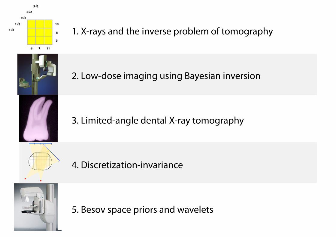
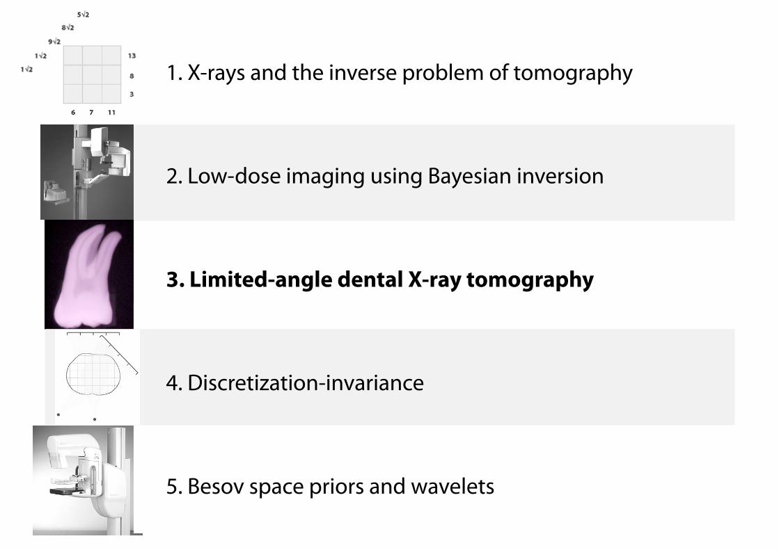
1. X-rays and the inverse problem of tomography

2. Low-dose imaging using Bayesian inversion

3. Limited-angle dental X-ray tomography

5. Besov space priors and wavelets

4. Discretization-invariance

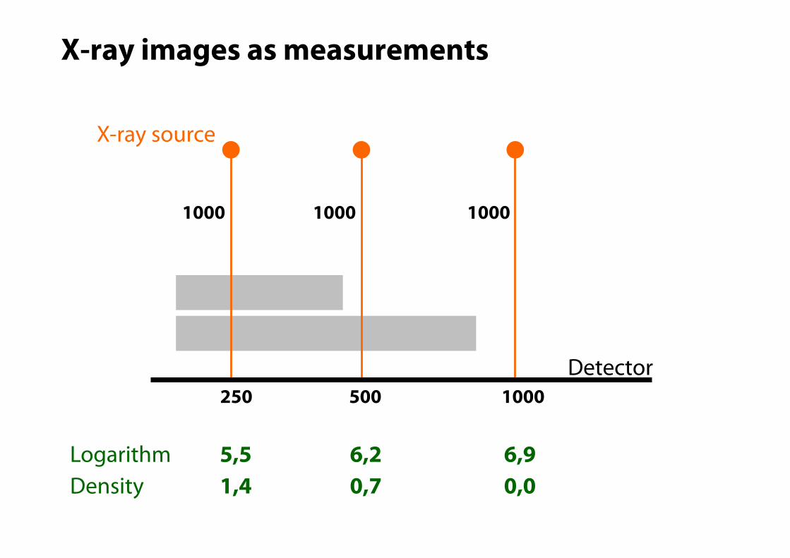
X-ray images as measurements

Detector

1000

1000

1000 1000

500 250

X-ray source

Logarithm 5,5 6,2 6,9 Density 1,4 0,7 0,0

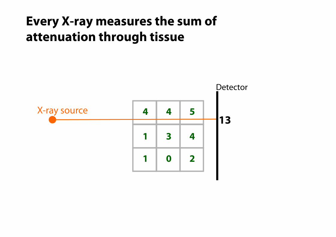
4 4 5

1 3 4

1 0 2

13 X-ray source

Detector

Every X-ray measures the sum of attenuation through tissue

4 4 5

1 3 4

1 0 2

11 7 6

13

8

3

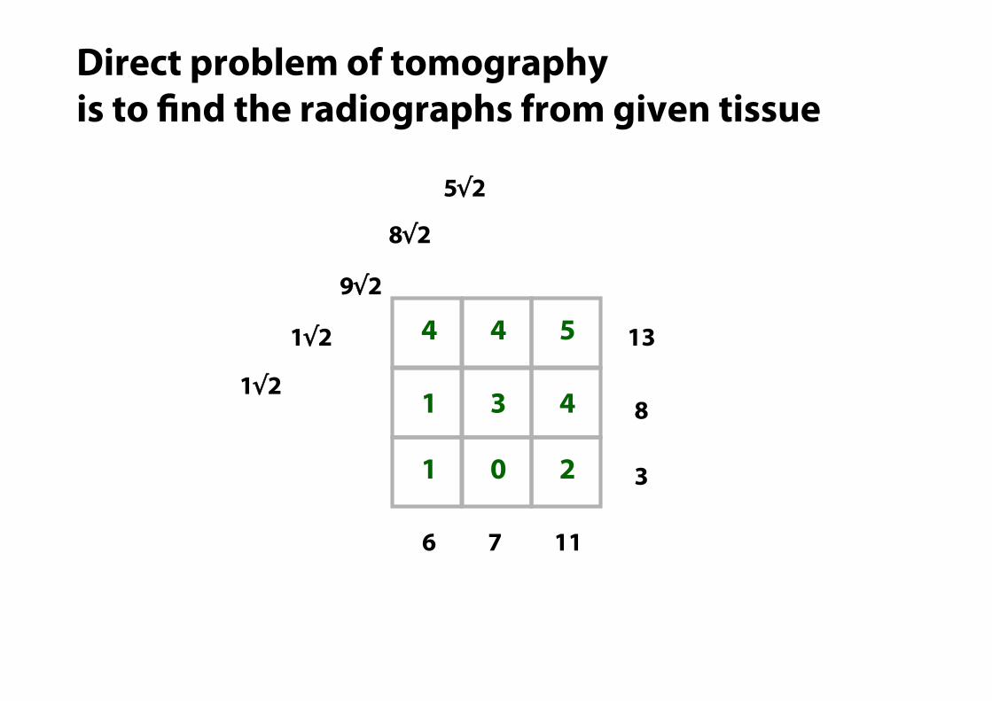
9√2

8√2

1√2

1√2

5√2

Direct problem of tomography is to !nd the radiographs from given tissue

11 7 6

13

8

3

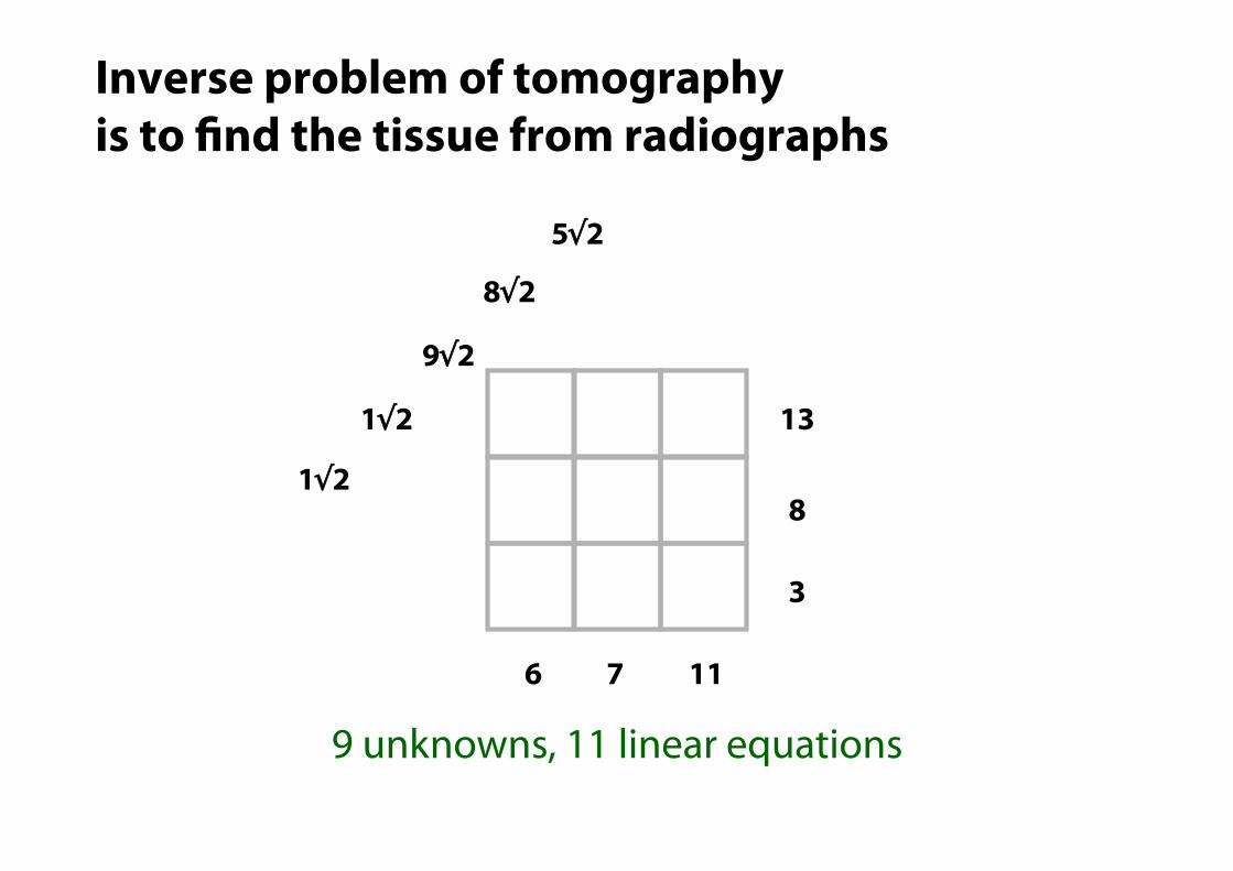
Inverse problem of tomography is to !nd the tissue from radiographs

9 unknowns, 11 linear equations

9√2

8√2

1√2

1√2

5√2

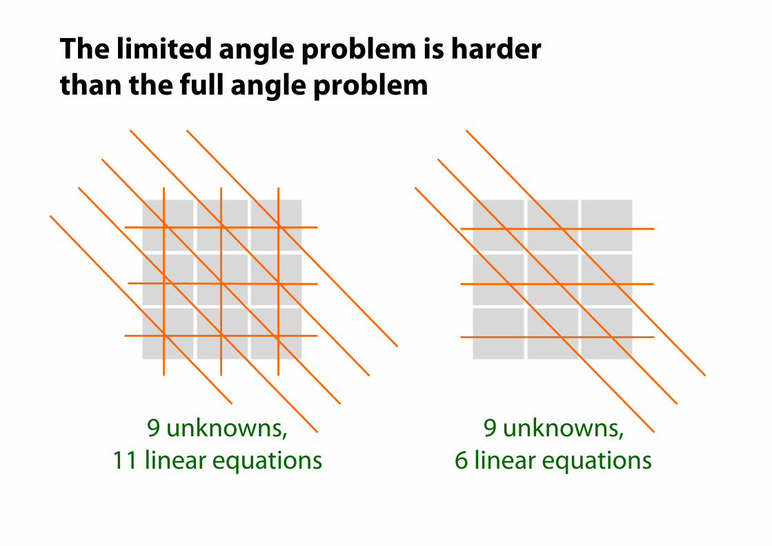
9 unknowns, 11 linear equations

9 unknowns, 6 linear equations

The limited angle problem is harder than the full angle problem

13

8

3

9√2

8√2

1√2 4 4 5

1 3 4

1 0 2

5 6 2

1 5 2

4 0 -1

9 1 3

1 0 7

3 0 0

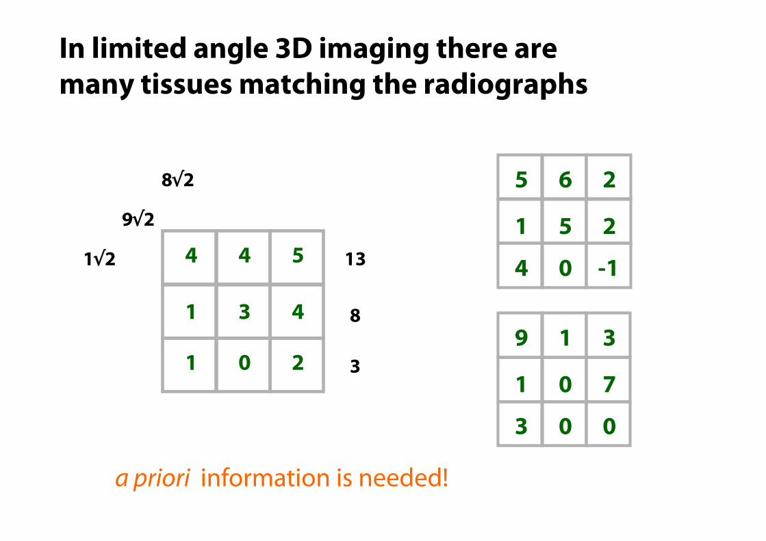
a priori information is needed!

In limited angle 3D imaging there are many tissues matching the radiographs

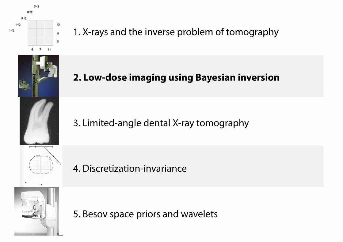
1. X-rays and the inverse problem of tomography

2. Low-dose imaging using Bayesian inversion

3. Limited-angle dental X-ray tomography

5. Besov space priors and wavelets

4. Discretization-invariance

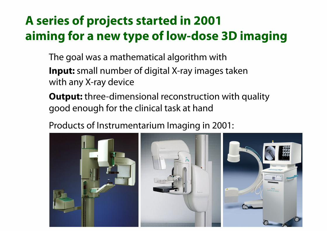
A series of projects started in 2001 aiming for a new type of low-dose 3D imaging

The goal was a mathematical algorithm with Input: small number of digital X-ray images taken with any X-ray device Output: three-dimensional reconstruction with quality good enough for the clinical task at hand

Products of Instrumentarium Imaging in 2001:

Academic members: Inverse problems research groups in University of Helsinki, University of Kuopio, Helsinki University of Technology and Tampere University of Technology

Industrial members: 2001-2002 Instrumentarium Imaging and Invers Ltd 2003-2004 GE Healthcare Finland 2005-2007 PaloDEx Group

Funding by TEKES and the companies.

Outcome: 12 peer-reviewed articles, 3 patents, algorithms for 3 commercial products

Essential history of the three projects:

~

m4

m5

m6

m2

m3

m1 x1 x4 x7

x2 x5 x8

x3 x6 x9

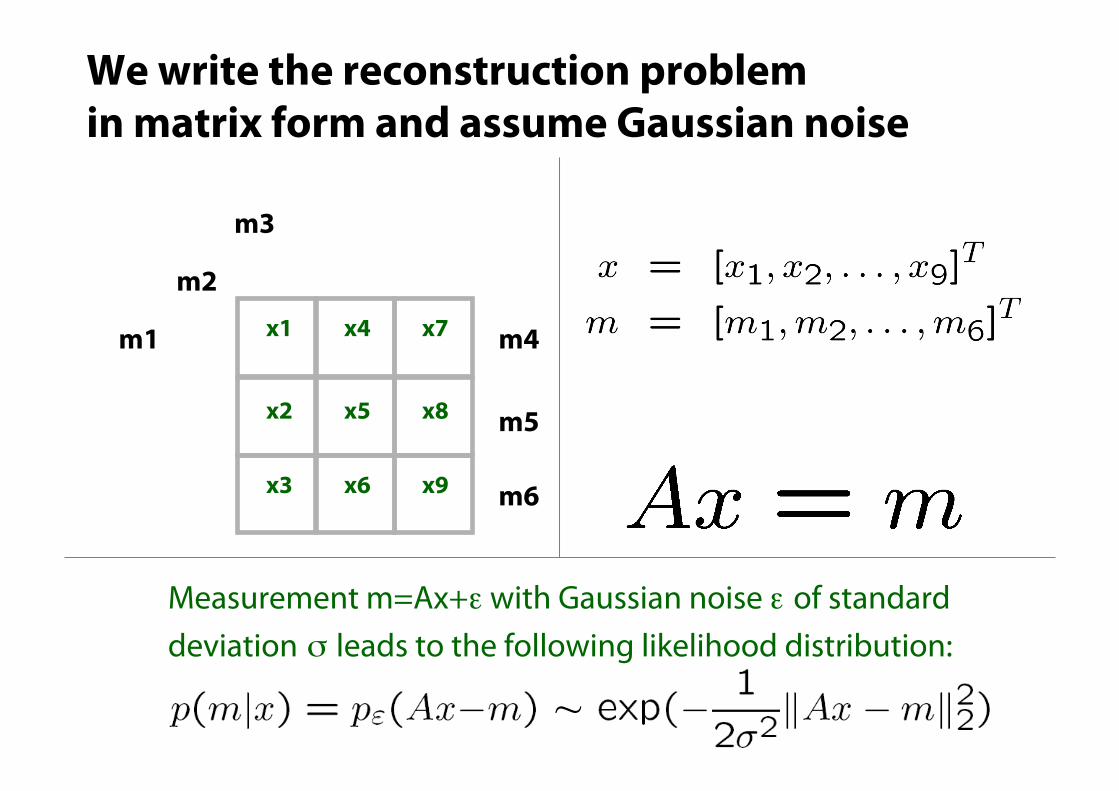
We write the reconstruction problem in matrix form and assume Gaussian noise

Measurement m=Ax+ε with Gaussian noise ε of standard deviation σ leads to the following likelihood distribution:

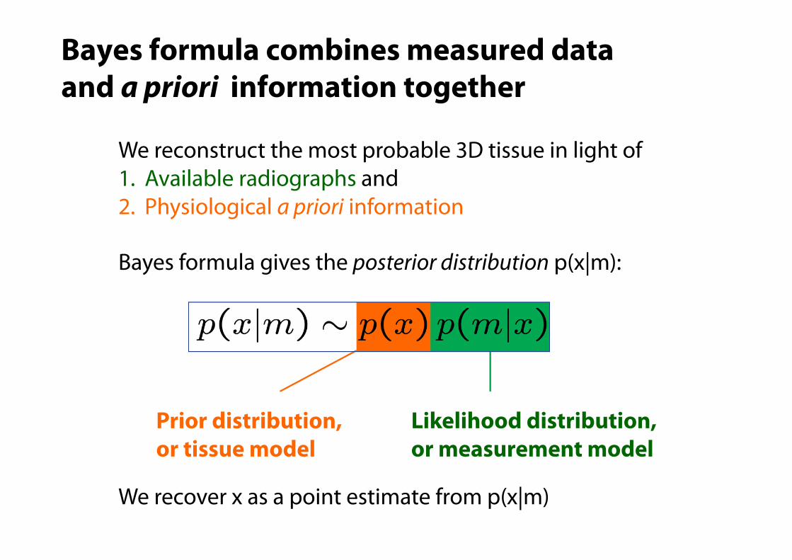
Bayes formula combines measured data and a priori information together

We reconstruct the most probable 3D tissue in light of 1.  Available radiographs and 2.  Physiological a priori information

Bayes formula gives the posterior distribution p(x|m):

We recover x as a point estimate from p(x|m)

Prior distribution, or tissue model

Likelihood distribution, or measurement model

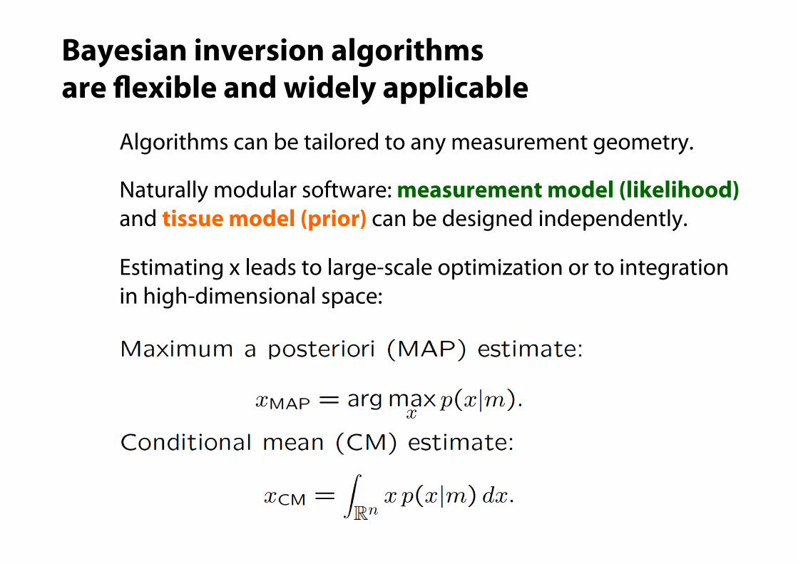
Algorithms can be tailored to any measurement geometry.

Naturally modular software: measurement model (likelihood) and tissue model (prior) can be designed independently.

Estimating x leads to large-scale optimization or to integration in high-dimensional space:

Bayesian inversion algorithms are "exible and widely applicable

1. X-rays and the inverse problem of tomography

2. Low-dose imaging using Bayesian inversion

3. Limited-angle dental X-ray tomography

5. Besov space priors and wavelets

4. Discretization-invariance

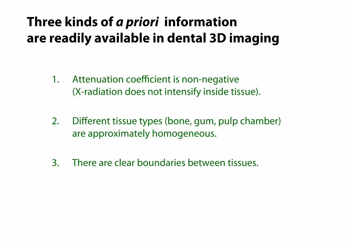
1.  Attenuation coefficient is non-negative (X-radiation does not intensify inside tissue).

2.  Different tissue types (bone, gum, pulp chamber) are approximately homogeneous.

3.  There are clear boundaries between tissues.

Three kinds of a priori information are readily available in dental 3D imaging

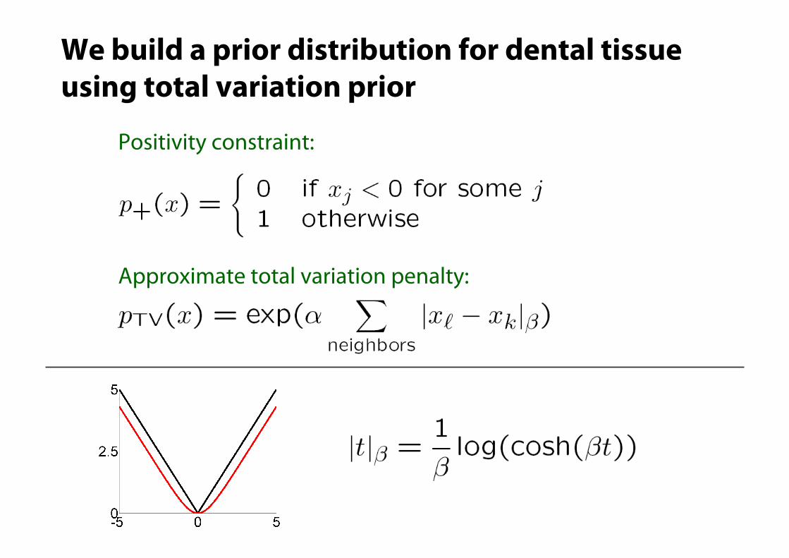
We build a prior distribution for dental tissue using total variation prior

Positivity constraint:

Approximate total variation penalty:

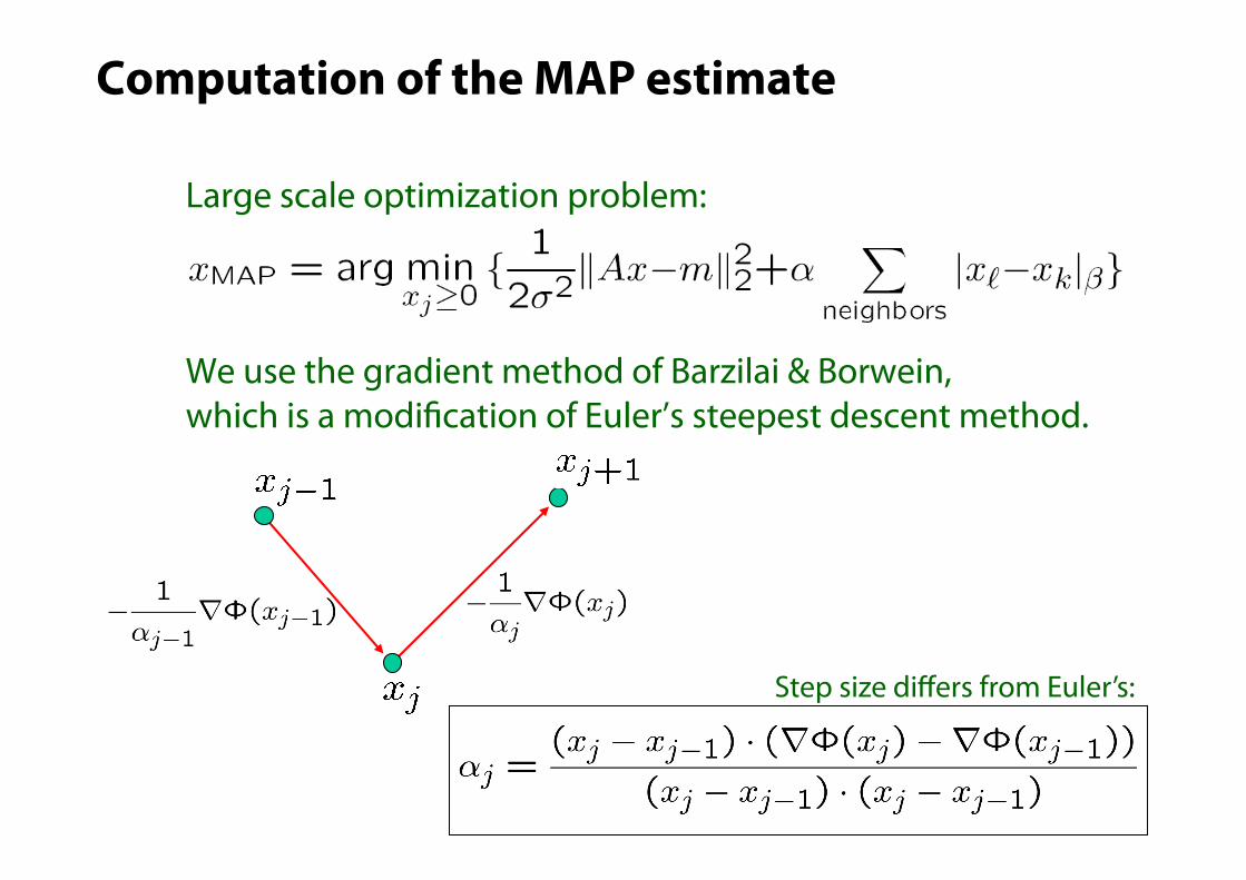
Computation of the MAP estimate

Large scale optimization problem:

We use the gradient method of Barzilai & Borwein, which is a modi#cation of Euler’s steepest descent method.

Step size differs from Euler’s:

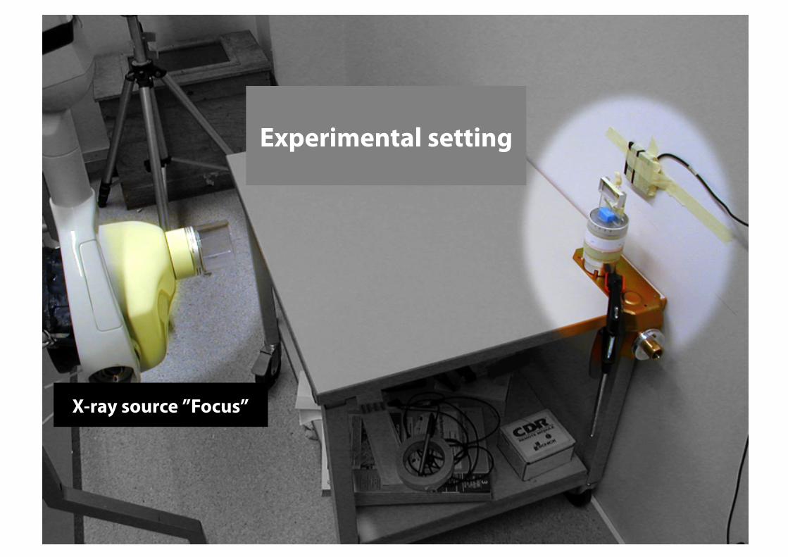
Experimental setting

X-ray source ”Focus”

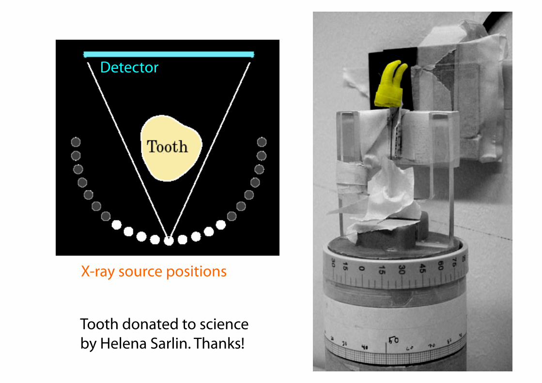
Detector

X-ray source positions

Tooth donated to science by Helena Sarlin. Thanks!

The projection images look like this

0 30 60 90

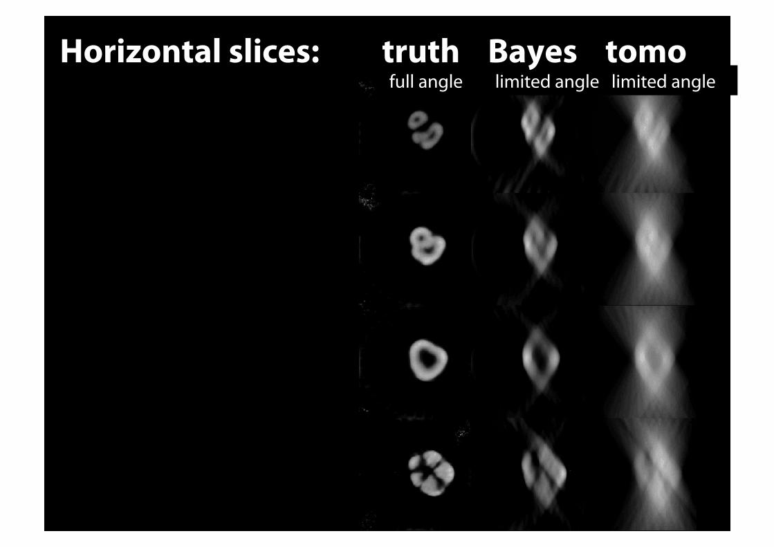
full angle limited angle limited angle Horizontal slices: truth Bayes tomo

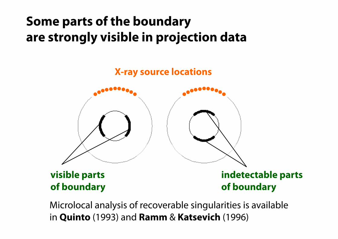
Some parts of the boundary are strongly visible in projection data

visible parts of boundary

indetectable parts of boundary

X-ray source locations

Microlocal analysis of recoverable singularities is available in Quinto (1993) and Ramm & Katsevich (1996)

full angle limited angle limited angle Vertical slices: truth Bayes tomo

Kolehmainen, S, Järvenpää, Kaipio, Koistinen, Lassas, Pirttilä, Somersalo (2003)

MAP Conditional mean (MCMC)

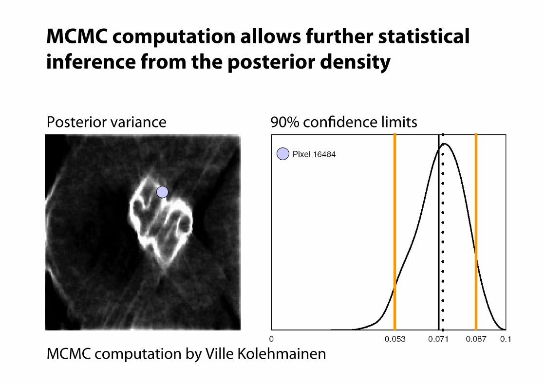
MCMC computation allows further statistical inference from the posterior density

Posterior variance 90% con#dence limits

MCMC computation by Ville Kolehmainen

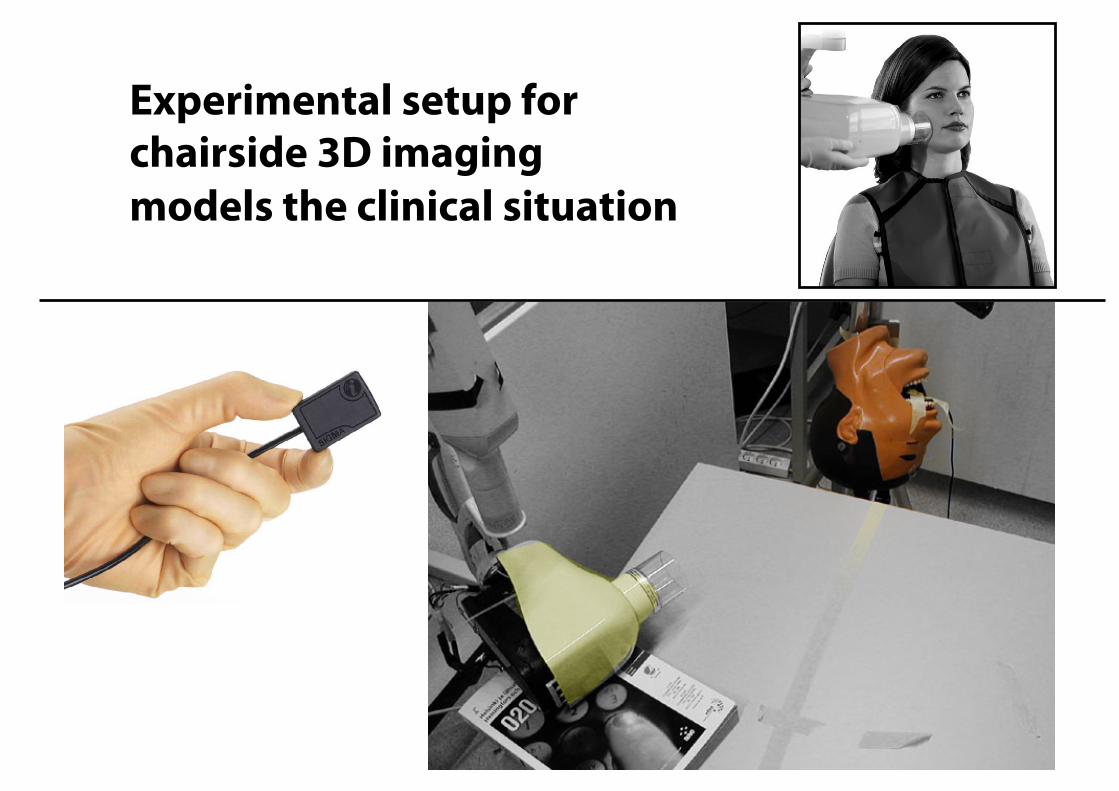
Experimental setup for chairside 3D imaging models the clinical situation

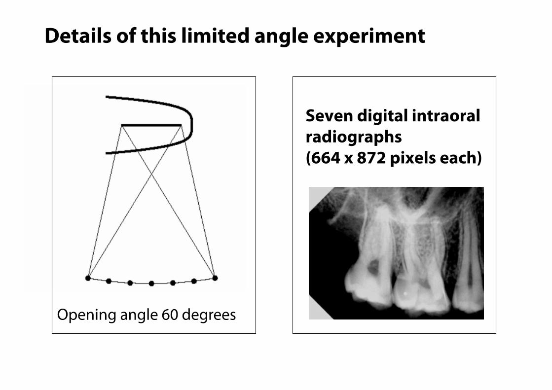
Details of this limited angle experiment

Seven digital intraoral radiographs (664 x 872 pixels each)

Opening angle 60 degrees

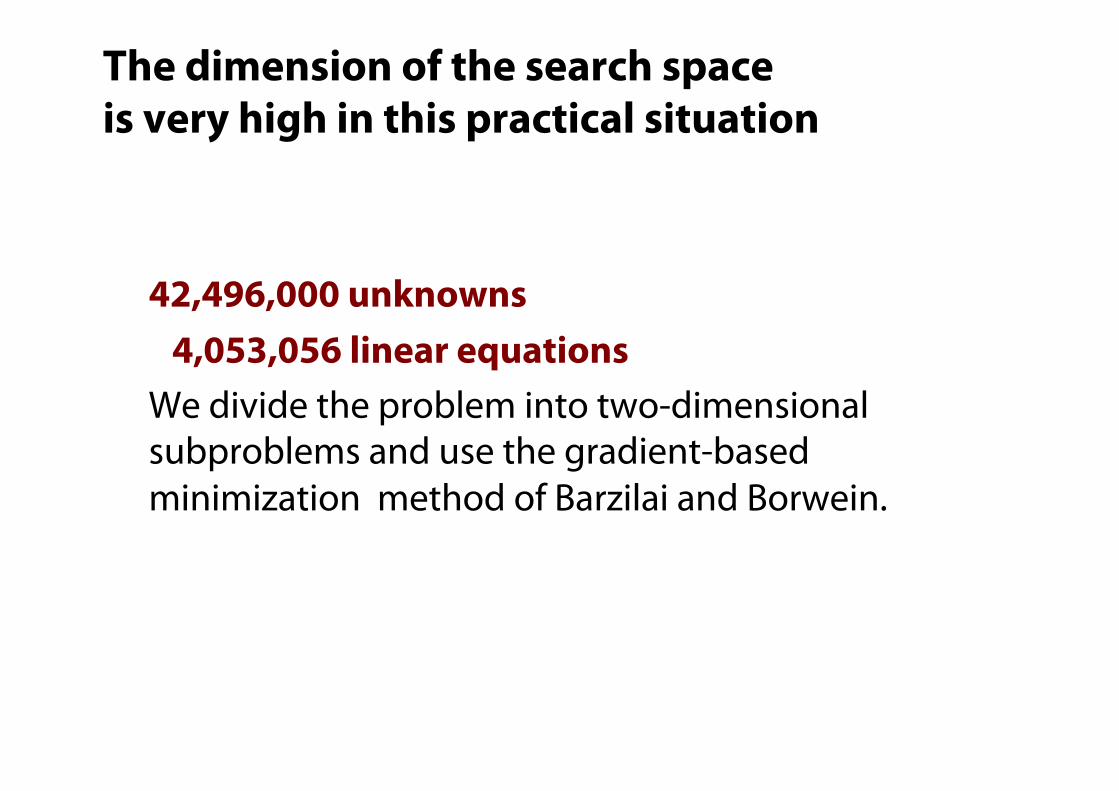
The dimension of the search space is very high in this practical situation

42,496,000 unknowns 4,053,056 linear equations We divide the problem into two-dimensional subproblems and use the gradient-based minimization method of Barzilai and Borwein.

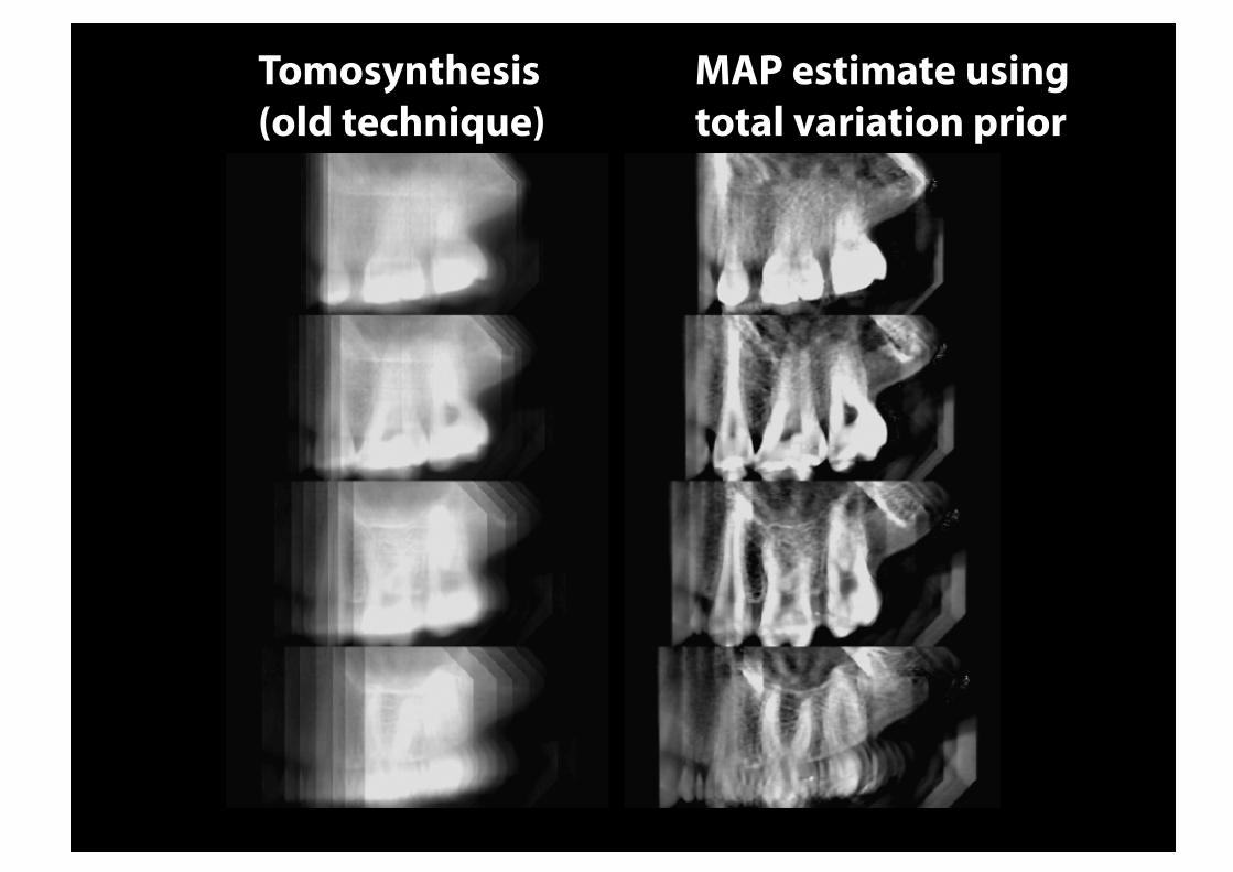
Tomosynthesis MAP estimate using (old technique) total variation prior

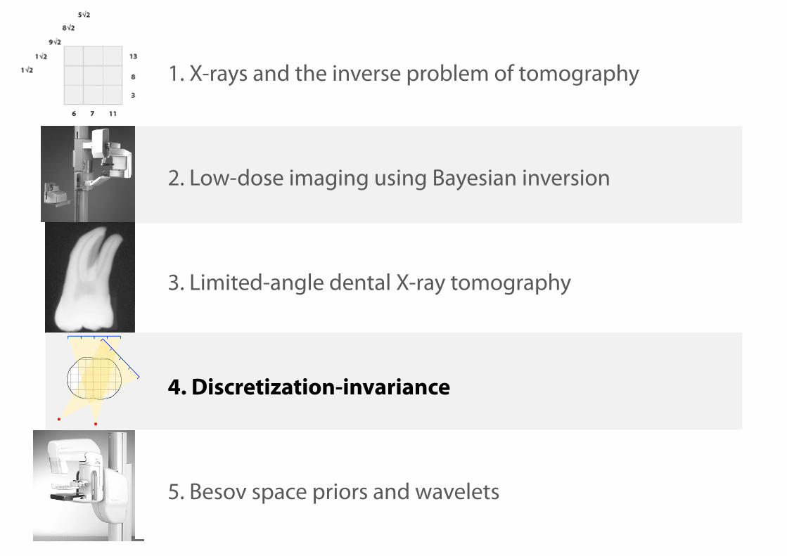
1. X-rays and the inverse problem of tomography

2. Low-dose imaging using Bayesian inversion

3. Limited-angle dental X-ray tomography

5. Besov space priors and wavelets

4. Discretization-invariance

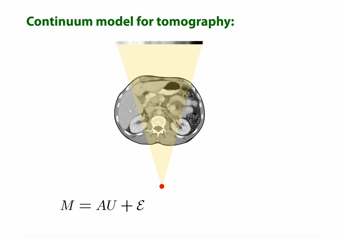
Continuum model for tomography:

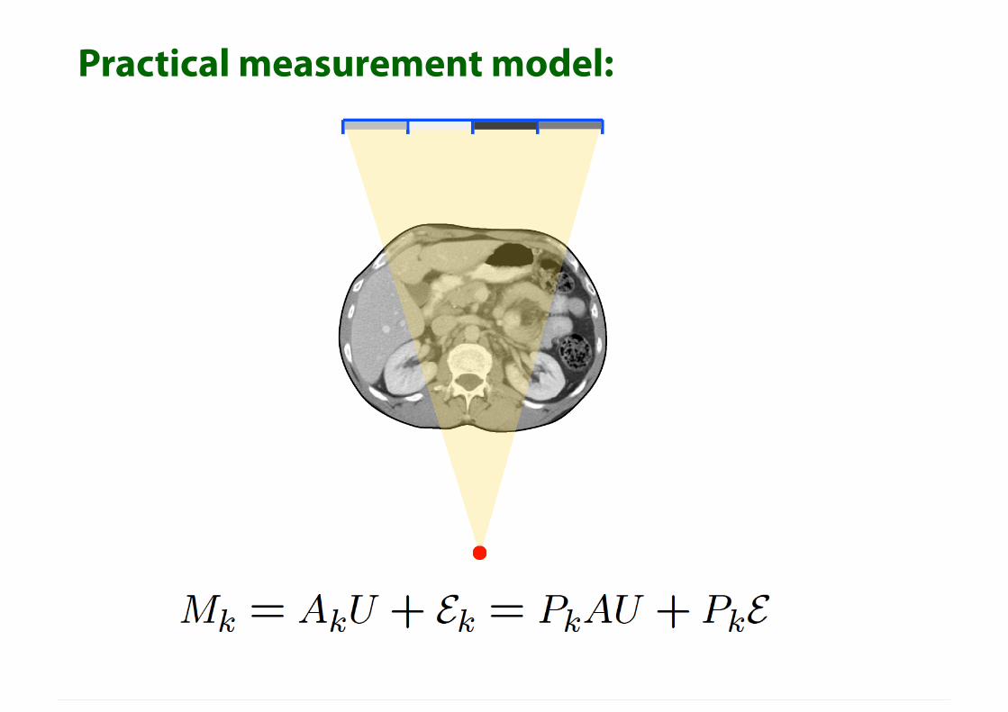
Practical measurement model:

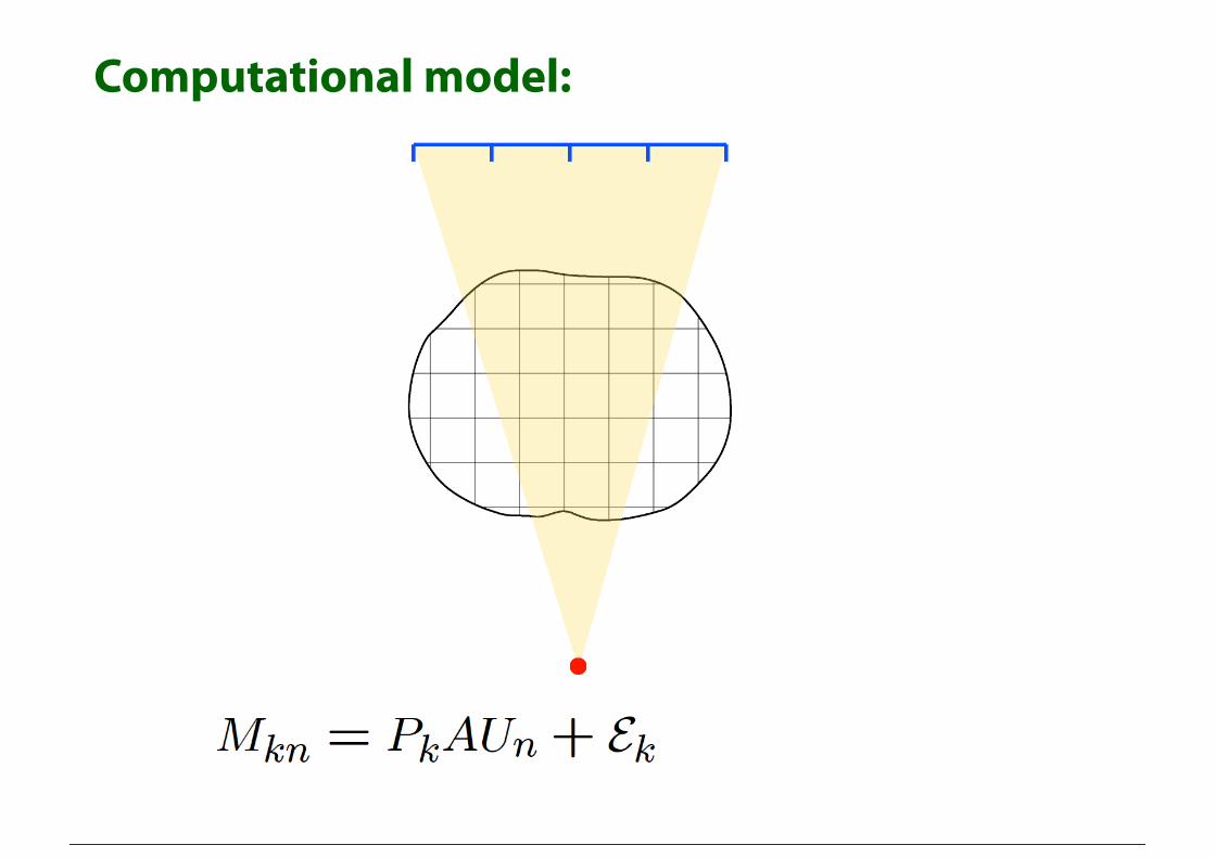
Computational model:

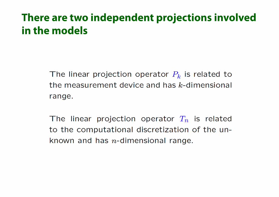
There are two independent projections involved in the models

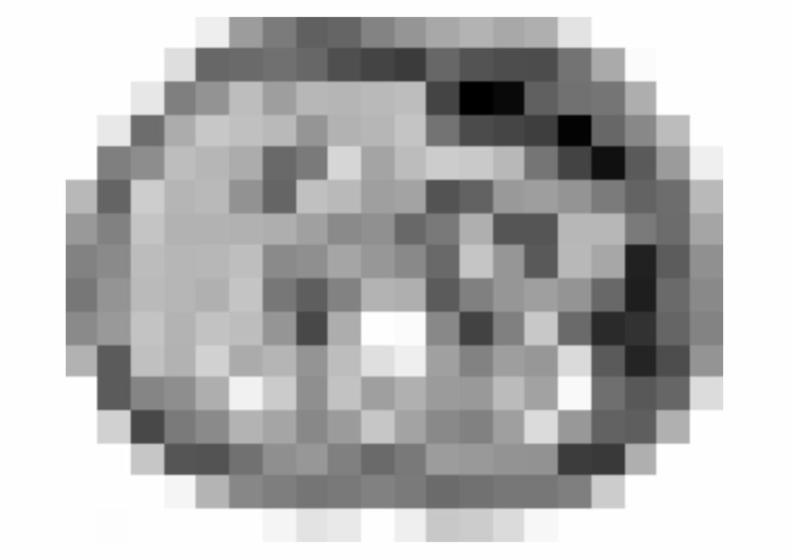
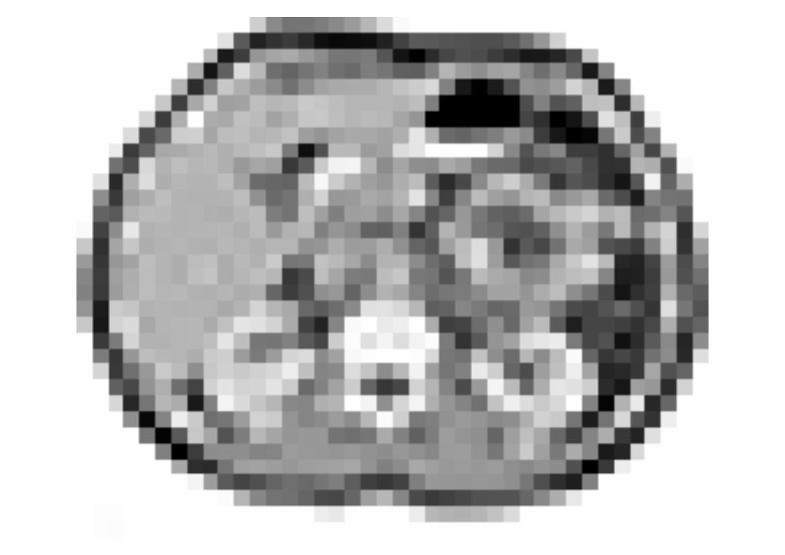
k=8

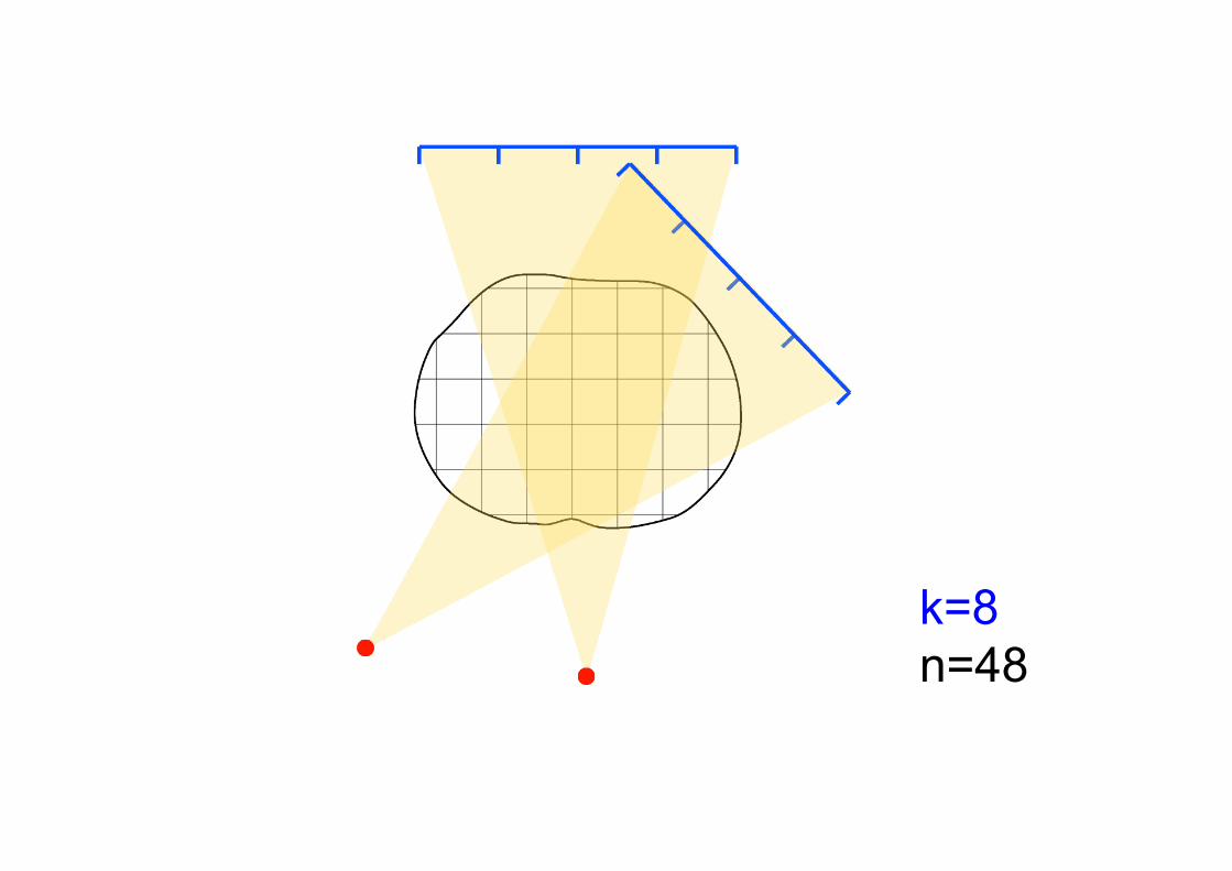
k=8 n=48

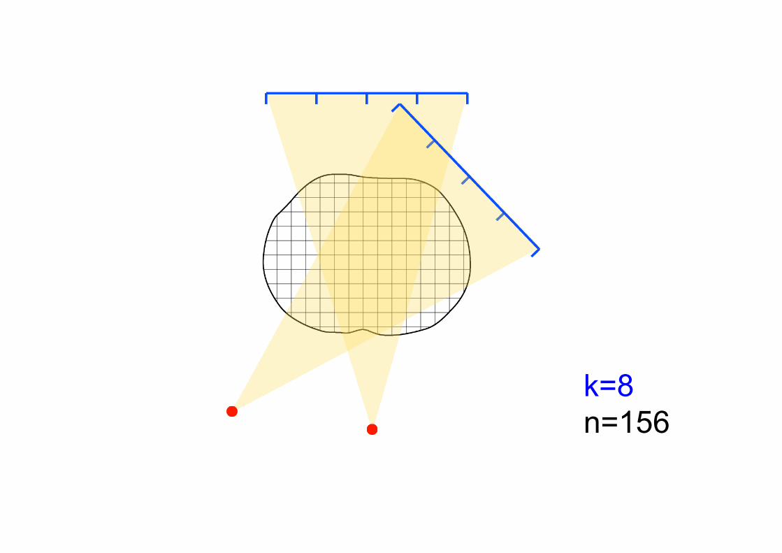
k=8 n=156

k=8 n=440

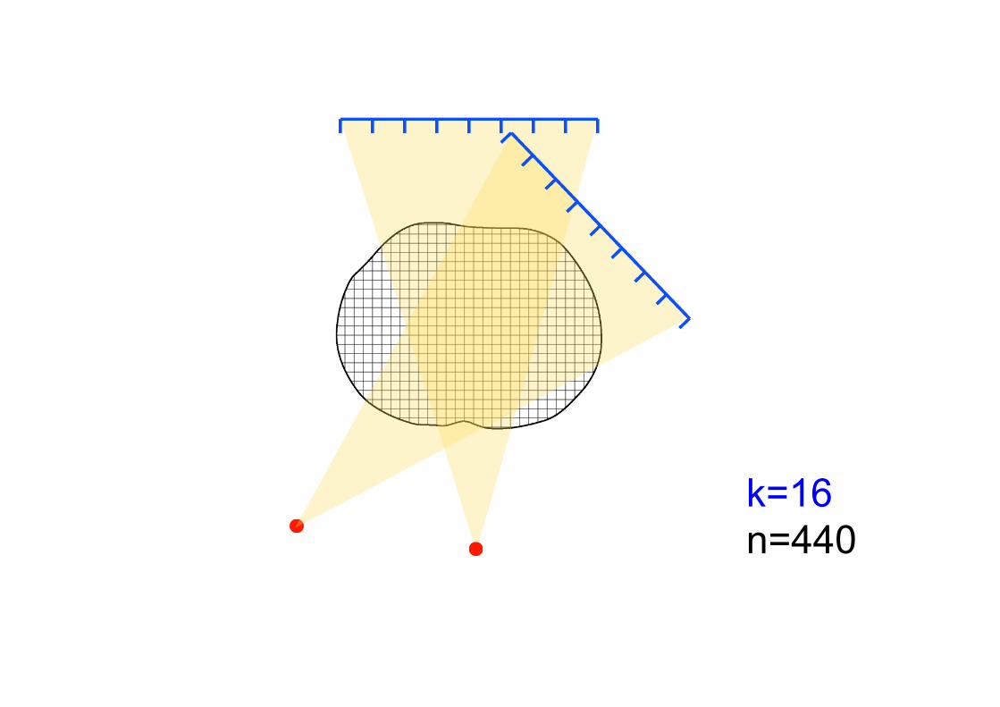
k=16 n=440

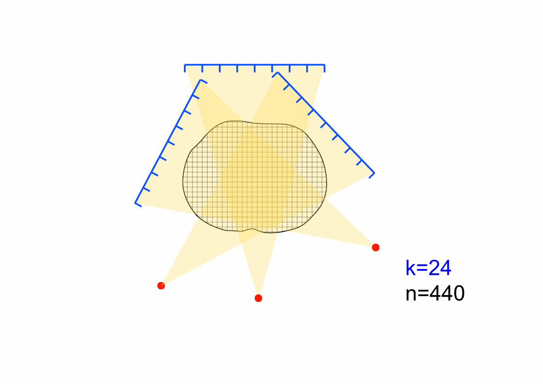
k=24 n=440

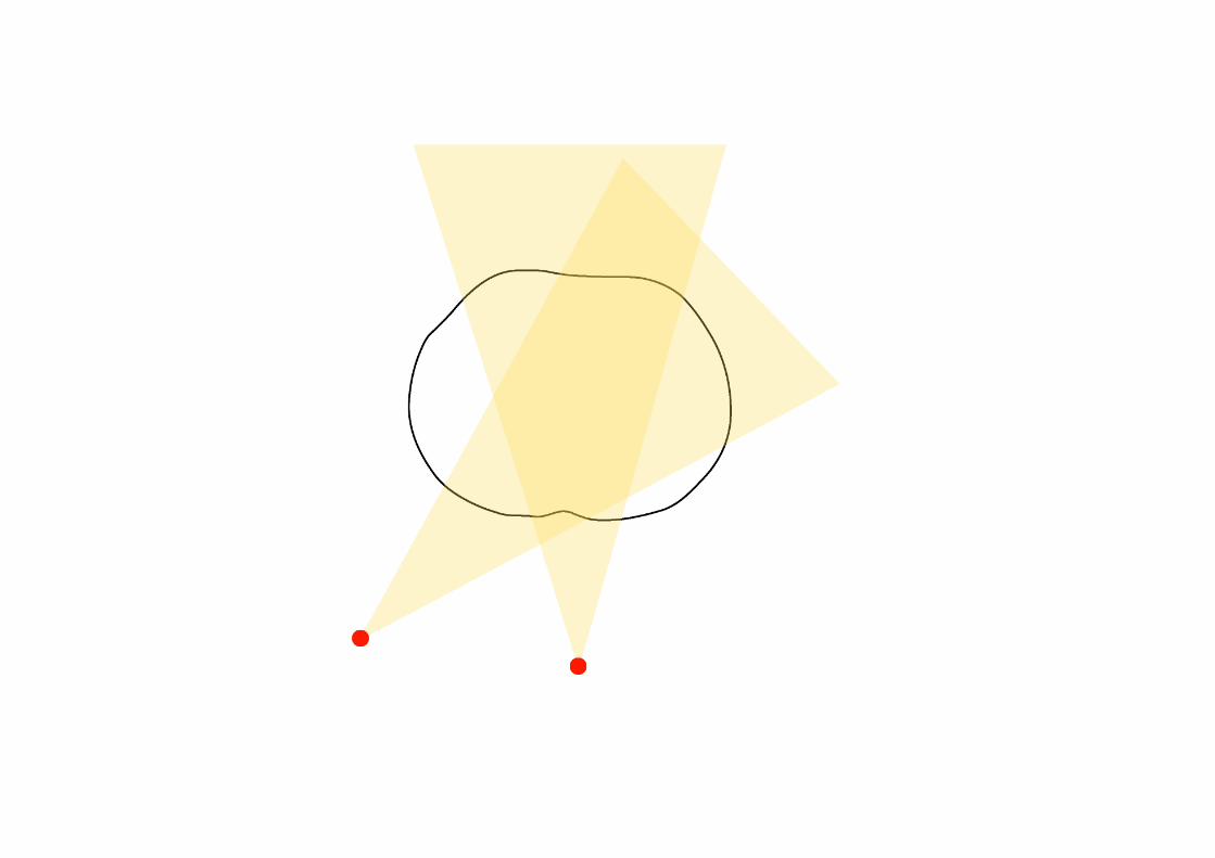
This is the central idea of studying discretization-invariance:

The numbers n and k are independent.

For the Bayesian inversion strategy to work, posterior estimates must converge as n or k or both tend to in!nity.

We arrived at these results suggesting that Besov space priors are the way to go

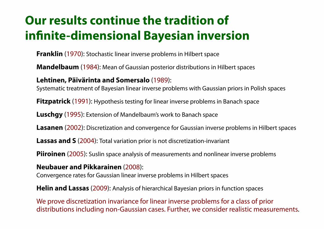
Our results continue the tradition of in!nite-dimensional Bayesian inversion

Franklin (1970): Stochastic linear inverse problems in Hilbert space

Mandelbaum (1984): Mean of Gaussian posterior distributions in Hilbert spaces

Lehtinen, Päivärinta and Somersalo (1989): Systematic treatment of Bayesian linear inverse problems with Gaussian priors in Polish spaces

Fitzpatrick (1991): Hypothesis testing for linear inverse problems in Banach space

Luschgy (1995): Extension of Mandelbaum’s work to Banach space

Lasanen (2002): Discretization and convergence for Gaussian inverse problems in Hilbert spaces

Lassas and S (2004): Total variation prior is not discretization-invariant

Piiroinen (2005): Suslin space analysis of measurements and nonlinear inverse problems

Neubauer and Pikkarainen (2008): Convergence rates for Gaussian linear inverse problems in Hilbert spaces

Helin and Lassas (2009): Analysis of hierarchical Bayesian priors in function spaces

We prove discretization invariance for linear inverse problems for a class of prior distributions including non-Gaussian cases. Further, we consider realistic measurements.

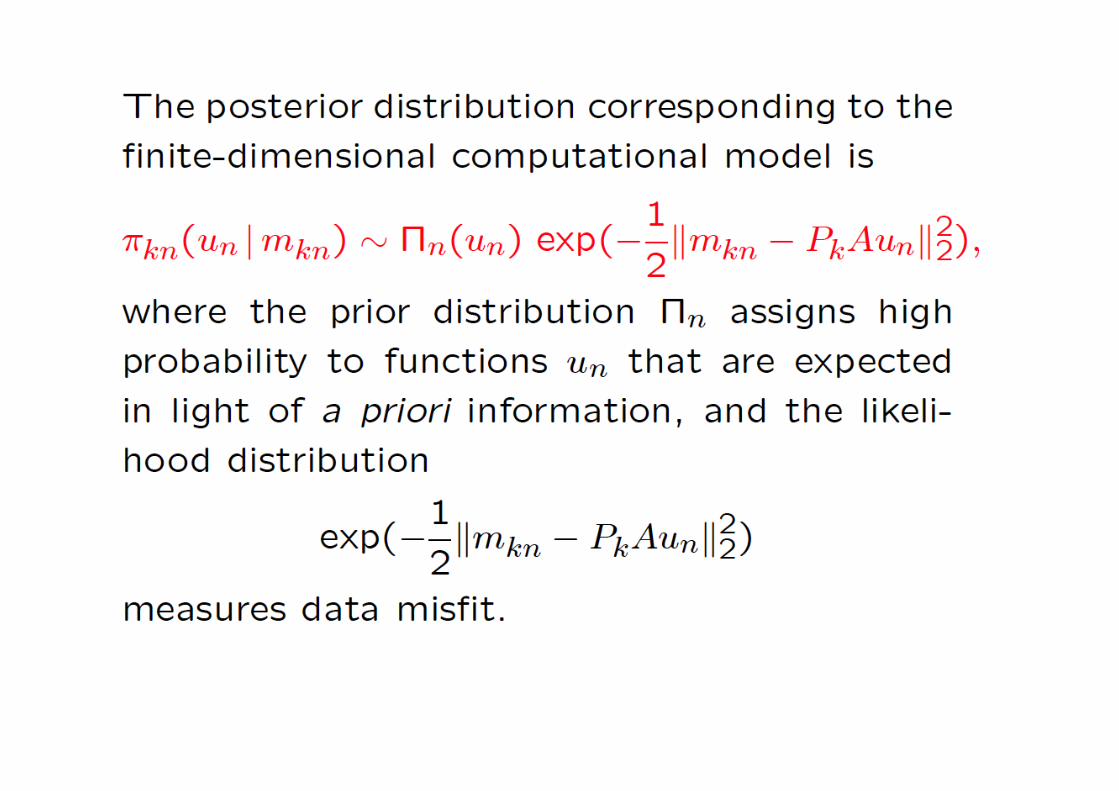
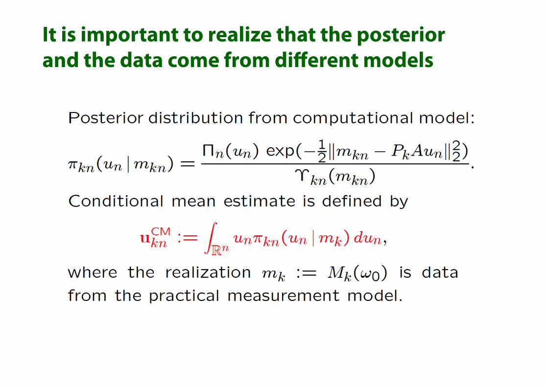
It is important to realize that the posterior and the data come from different models

1. X-rays and the inverse problem of tomography

2. Low-dose imaging using Bayesian inversion

3. Limited-angle dental X-ray tomography

5. Besov space priors and wavelets

4. Discretization-invariance

Wavelet transform divides a function into details at different scales

We introduce a convenient renumbering of the basis functions

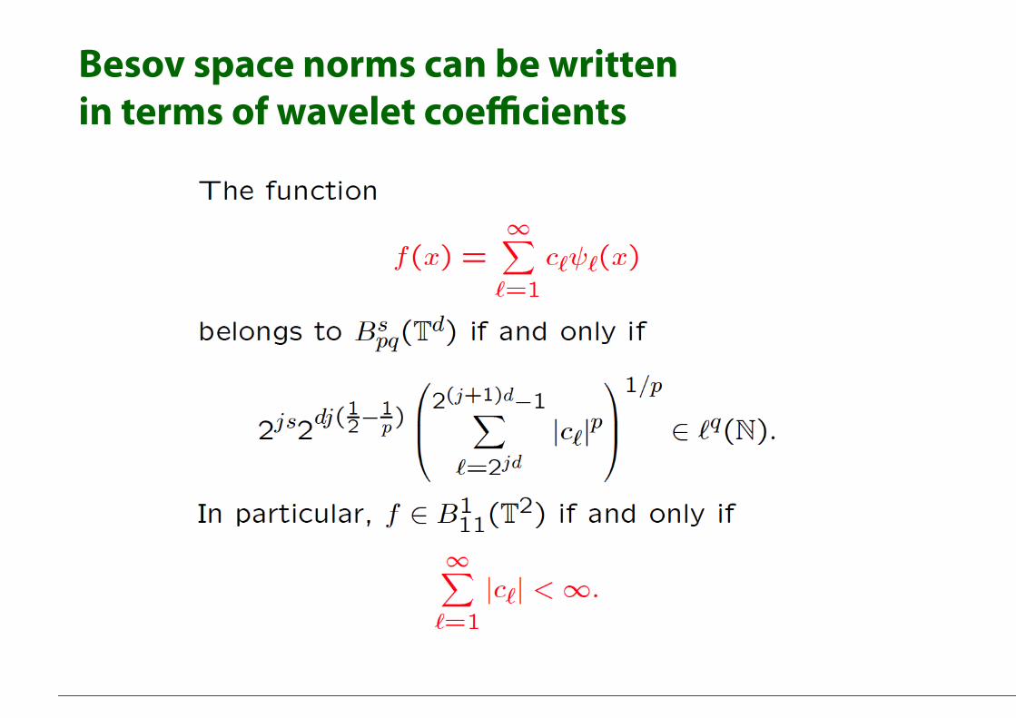
Besov space norms can be written in terms of wavelet coefficients

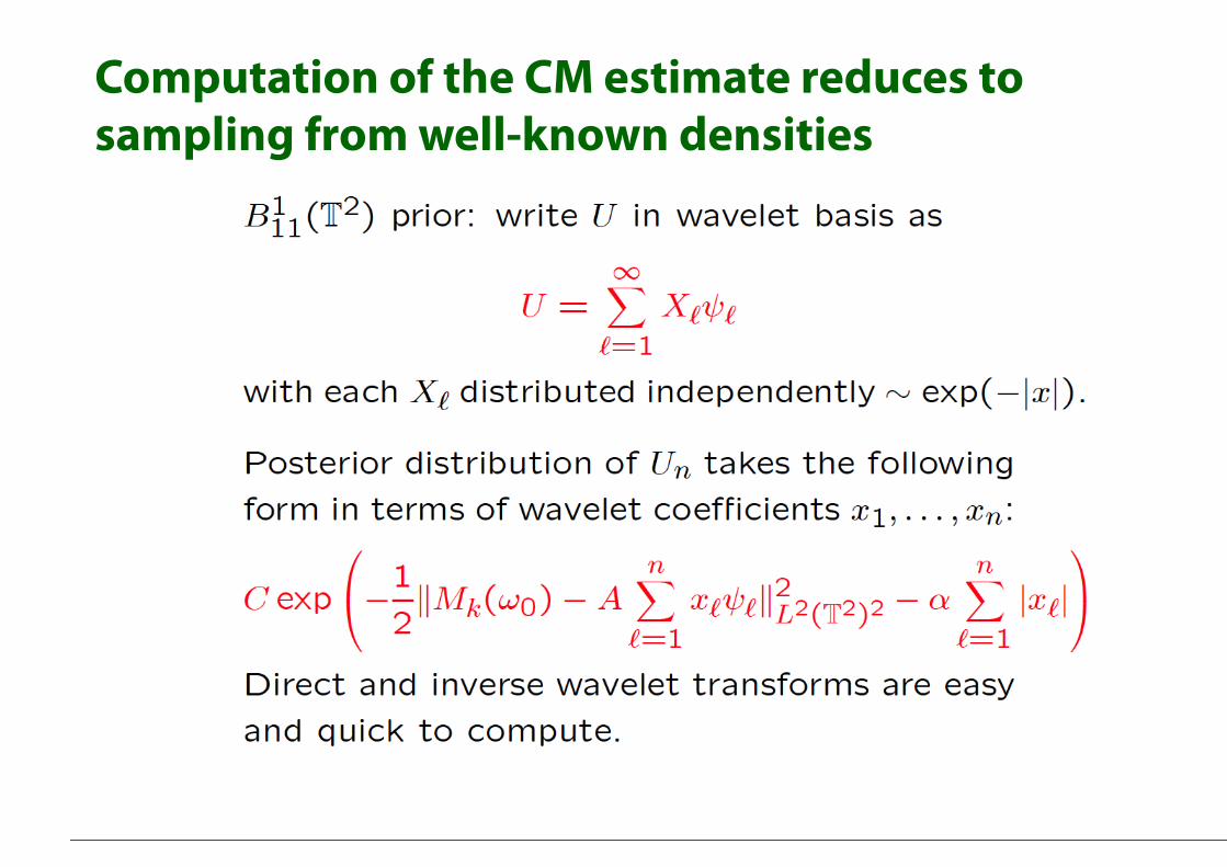
Computation of the CM estimate reduces to sampling from well-known densities

Limited angle tomography results for X-ray mammography

[Rantala et al. 2006] Thanks to GE Healthcare

Tomosynthesis

MAP estimate, Besov prior, p=1.5=q and s=0.5

Local tomography results for dental X-ray imaging; data measured from specimen

Niinimäki, S and Kolehmainen (2007) Thanks to Palodex Group

Lambda-tomography MAP using Besov prior with p=q=1.5 and s=0.5

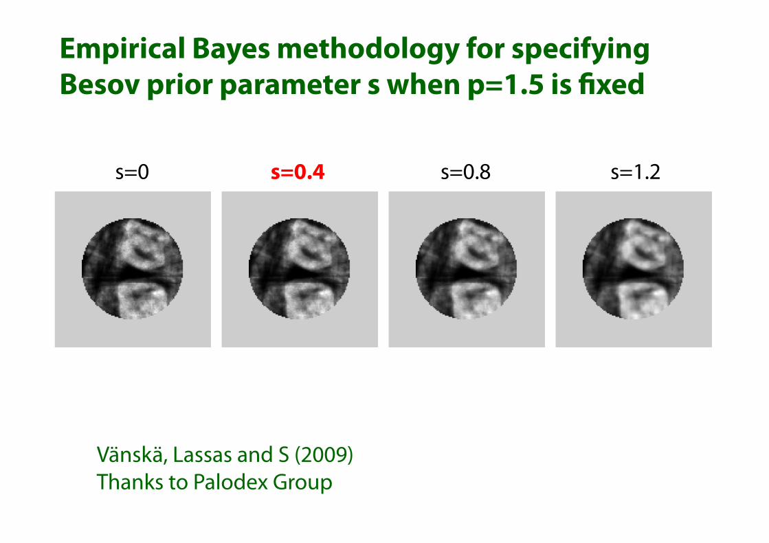
Empirical Bayes methodology for specifying Besov prior parameter s when p=1.5 is !xed

Vänskä, Lassas and S (2009) Thanks to Palodex Group

s=0 s=0.4 s=0.8 s=1.2

The success of total variation regularization makes the choice of Besov parameters s=1 and p=q=1 especially interesting.

However, computations become more involved as the objective function is nonsmooth.

First attempt: Daubechies 7 mother wavelet

We chose a simple one-dimensional deconvolution problem for testing TV and Besov priors. Left: Total variation regularization (equivalent to MAP) Right: MAP with Besov prior when s=1 and p=q=1. We use Daubechies 7 mother wavelet since it is smooth enough to belong to the Besov space. This is joint work with V Kolehmainen, M Lassas and K Niinimäki.

Here s=1 and p=q=1. Dimension n=64

Next we decided to use Haar wavelet to preserve edges.

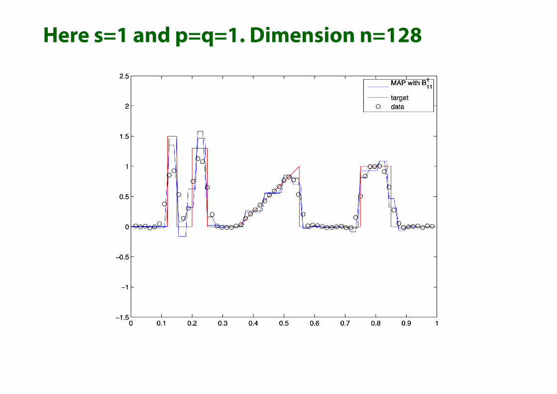
Here s=1 and p=q=1. Dimension n=128

Here s=1 and p=q=1. Dimension n=256

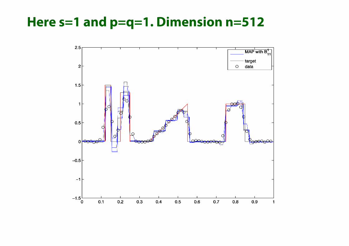
Here s=1 and p=q=1. Dimension n=512

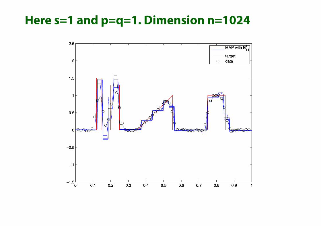
Here s=1 and p=q=1. Dimension n=1024

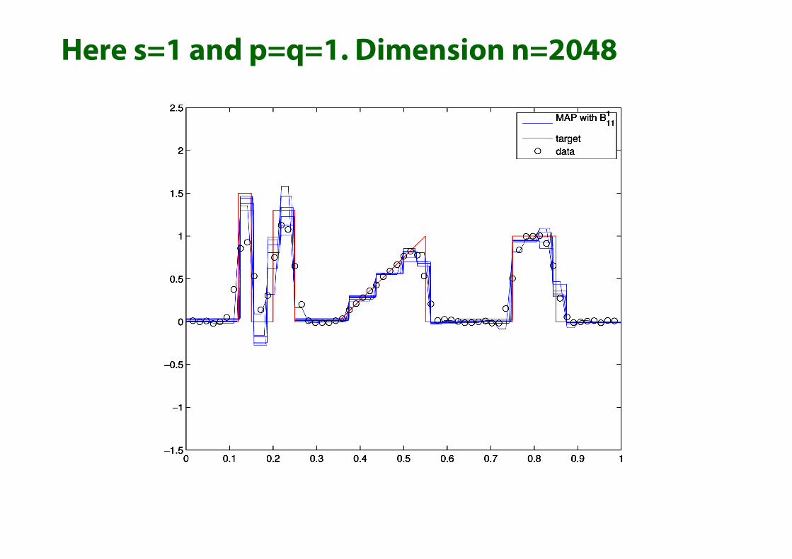
Here s=1 and p=q=1. Dimension n=2048

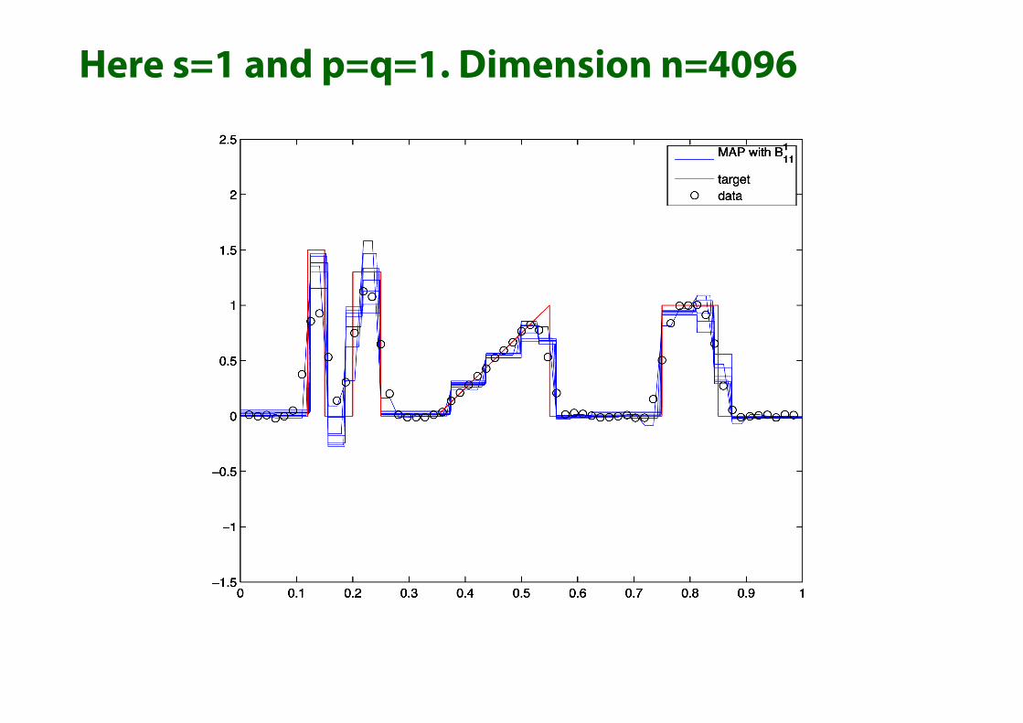
Here s=1 and p=q=1. Dimension n=4096

Our plan is to continue the study of Besov priors.

Next steps include MCMC computation and moving from one-dimensional examples to two-dimensional problems.