Chapter 4

Optimising landscape configuration to enhance

habitat suitability for species with contrasting

habitat requirements

An edited version of Holzkämper et al. 2006. Ecological Modelling, published.

Abstract

Heterogeneity of agricultural landscapes is supposed to be of significant importance for species

diversity in agroecosystems. However, land-use-pattern changes may lead to an increase in

suitable habitat for some species, but to habitat deterioration for other species with opposing

habitat requirements. To investigate the effects of land-use changes on different species’ habitat

suitabilities and to allow a trade-off between management objectives, we applied a spatial

optimisation model. In this paper we present a new approach that integrates a neighbourhood

dependent multi-species evaluation of land-use patterns into an optimisation framework for

generating goal-driven scenarios. It is implemented using a genetic algorithm approach that aims

at maximising habitat suitability of three selected bird species (Middle-Spotted Woodpecker,

Wood Lark, Red-Backed Shrike) by identifying optimum agricultural land-use patterns. The

evaluation of habitat suitability is based on landscape metrics calculated within the species’ home

ranges to incorporate the effects of species responses to landscape pattern on a coarser scale. The

main focus of this study is to explore the potential of this approach for conservation management

on the basis of a case study. We investigate where habitat requirements oppose, where they

coincide and how a landscape optimised simultaneously for all target species should be

characterised. We found that all species would benefit from an increase of deciduous and

coniferous forest, a decrease of cropland and grassland in the study area and more heterogeneous

land-use patterns (smaller patches, more diversity of land-use types). Habitat requirements of

Chapter 4 19

Red-Backed Shrike contrast most to those of the other two species with respect to landscape

composition and configuration.

4.1 Introduction

Landscape structure is thought to have important influences on various ecosystem functions (e.g.

biodiversity (Weber et al. 2001, Weibull et al. 2003), nutrient cycles (Seppelt & Voinov 2002,

Lenhart et al. 2003), and water balance (Bormann et al. 1999, Bellot et al. 2001)). In this paper,

we focus on the impacts of landscape structure on habitat suitability for different bird species. As

species habitat requirements differ, changes may have positive effects on some species and

negative effects on other species. For example, some species like the Middle-Spotted Woodpecker

prefer core habitats, while other species such as the Red-Backed Shrike depend on boundary

structures like forest edges or hedges (Latus et al. 2004). Furthermore, some species may use

different habitat types for different activities such as breeding and foraging. Land-use changes

may therefore lead to an increase in suitable habitat for one species, but to habitat loss and

fragmentation for another species with opposing habitat requirements. As bird species are known

to respond to habitat factors at coarser spatial scales, land-use patterns within a certain radius need

to be considered for evaluating habitat suitability (Freemark & Merriam 1986, Graf et al. 2005).

Scenario analysis can be applied to analyse the effects of land-use changes on habitats for

different species. However, to methodically approximate an optimum landscape pattern with

respect to a certain goal, a spatially explicit optimisation approach must be employed. This

technique allows one to incorporate trade-offs between different management objectives. Spatial

optimisation methods have mostly been used in the field of timber and wildlife management

(Thompson et al. 1973, Nevo & Garcia 1996, Bevers et al. 1997, Church et al. 2000, Loehle 2000,

Hof et al. 2002), for selecting wildlife reserves (Pressey et al. 1995, Polansky et al. 2000, Cabeza

& Moilanen 2003, Strange et al. 2006) or for optimising crop yields given ecological constraints

(Seppelt 2000, Seppelt & Voinov 2002). Many applications of optimisation approaches are

spatially explicit, but only a few of them take into account neighbourhood dependencies. Bevers

& Hof (1999) optimise habitat configuration resulting from forest management with respect to

wildlife edge effects. A similar approach was used by Moore et al. (2000), where population

viability was optimised over ten decision periods based on a very simple landscape. Likewise,

Loehle (2000) minimises the impact of timber harvest on edge-sensitive bird species while

maximising timber harvest. This study is also based on a very simple grid landscape. Venema et

al. (2005) optimise forest structures with respect to certain landscape metrics.

In this paper, we present a new approach that integrates a neighbourhood dependent multi-species

evaluation of land-use patterns into an optimisation framework for generating goal-driven

Chapter 4 20

scenarios. We need to incorporate neighbourhood effects due to the dependencies of species’

habitat quality on the characteristics of surrounding habitat. Thus, we chose to implement our

model using a genetic algorithm, which is known to be capable of handling very complex

optimisation problems. Our optimisation model aims to maximise habitat suitability for three

selected bird species by identifying optimum agricultural land-use patterns. Bird species with

contrasting habitat requirements and preferences in habitat structure were chosen as target species

to investigate the different effects of land-use changes. In contrast to the approach of Venema et

al. (2005), where landscape-level metrics define the optimisation goal, our model uses cumulative

habitat suitabilities estimated for the study area to determine the optimisation goal. The evaluation

of these habitat suitabilities is based on static variables like soil types or climate factors and land-

use patterns quantified by landscape metrics (McGarigal et al. 2002). These metrics are estimated

within the species’ home ranges. Thus land-use patterns are optimised for the three species on a

territorial scale. The optimisation model approach allows us to analyse how weighting for selected

species affects the composition and configuration of optimised landscapes. The main focus of this

paper is to explore the potential of this approach for conservation management on the basis of a

case study. To do this, we investigate where species habitat requirements oppose and where they

coincide, and how a landscape optimised for all target species should be characterised.

4.2 Methodological concept

Our optimisation model is designed to implement trade-offs between different management

objectives, taking into account spatial configurations of landscape elements. It was used to detect

optimum landscape patterns for several species with contrasting habitat requirements. With this

approach, we want to analyse how an improvement of habitat suitability for one species affects

other species’ habitat suitability. Thus the optimisation task is to maximise the weighted sum of

habitat suitabilities of all species in the study area by identifying optimum spatial configurations

of agricultural land-use patterns. As this is quite a complex combinatorial problem, we apply a

genetic algorithm approach, which is known to be a robust method for gradient-free optimisation

(Goldberg 1989). We utilised the C++ genetic algorithm library GALib 2.4.6 by Wall (1996). The

results of logistic regression habitat suitability modelling are fed into the optimisation model to

evaluate the optimisation goal. To minimise the computational effort and avoid unrealistic land-

use patterns we defined model units as contiguous cells of identical land use. These model units

correspond to patches of agricultural fields, grassland and forest that are assumed to be managed

as entire units. Within the model units all grid cell values are changed en bloc.

Chapter 4 21

Habitat suitability modelling procedure

Statistical habitat suitability models were developed using logistic regression based on grid data

of the study area with 40 m resolution. As only presence point data was available for the target

species, random sets of pseudo-absence data were generated that were of equivalent size to those

in the actual presence data set. This method was chosen as it results in coefficients for all

variables that can be used for predicting habitat suitability under changed conditions in the

optimisation model. To avoid bias through spatial autocorrelation we excluded all presence points

where the home ranges overlapped. The selection of pseudo-absence data had to be done several

times because different samples could result in different models. To prevent pseudo-absence

points from overlapping with presence points, the selection was restricted by a mask layer, where

species’ occurrences buffered with the home range radius were excluded. For all data points

(presence and pseudo-absence), the local values of static habitat variables (e.g. elevation, slope,

proportion of soil texture, precipitation, sunshine duration, temperature) were stored. To test the

effects of structural landscape aspects on habitat suitability, landscape metrics (McGarigal et al.

2002) were calculated for each of these points within a radius that corresponds to the species’

home ranges. We incorporated the metrics largest patch index on the landscape level as well as

class area and edge density on class level in the habitat suitability modelling. We chose these

rather simple metrics as they have relatively high explanatory power and interpretability

(Tischendorf 2001). The largest patch index quantifies landscape homogeneity. Edge density is

given by the class length of edge segments (m) per hectare, while class area is simply the area of a

certain class per hectare. Furthermore, we used the patch cohesion metric at the class level, as this

metric incorporates class area and class fragmentation (Schumaker 1996). Patch cohesion

approaches zero as class area decreases and becomes increasingly subdivided and it increases

monotonically as class area increases until an asymptote is reached near the percolation threshold

(McGarigal et al. 2002). We also introduced an edge sum metric, which is the sum of edge cells of

one land-use type bordering a certain other land-use type, to include the effects of edges between

two specific land-use classes.

In the analysis, a set of uncorrelated potential habitat variables was chosen for each species. As

class area and patch cohesion of one land-use class are necessarily highly correlated, we tested the

relevance of each in separate analyses. One thousand pseudo-absence samples were drawn and

based on the presence data and multiple pseudo-absence data sets, 1000 logistic regression models

were calculated for each species by using a stepwise variable selection procedure (forward and

backward variable selection; Harrell 2001; Reineking & Schröder 2006). The step-function selects

a model according to the AIC (Akaike’s Information Criterion), which corresponds to a

penalisation term, of 2 which is equivalent to an α-level of 0.157 (Reineking & Schröder 2006).

Chapter 4 22

To allow a direct interpretation of model coefficients, all independent variables were scaled. The

coefficients of the most frequently occurring model were chosen and averaged to result in the

model used for predicting habitat suitabilities in the optimisation. Standard deviations for the

coefficients are standard errors of averaged estimates. To evaluate the averaged model, AUC (area

under the ROC-curve) was evaluated based on the 1000 samples. For model predictions, the

variable values were scaled with the averaged mean and the averaged standard deviation derived

from the data sets of the source models.

Model formulation of optimisation problem

As genetic algorithms (GA) are based on the principles of evolution, we need to perform the

following steps for coding an optimisation procedure with a GA:

a) Definition of ‘genome’: The subject of the optimisation needs a representation of

a certain data structure within the genetic algorithm. This representation is called

a ‘genome’ or ‘individual’ in this context. Evolution acts on a ‘population’ of

‘genomes’, where each ‘genome’ has slightly different characteristics. These

characteristics are equivalent to the ‘genes’ in a ‘genome’. The ‘allele’ set

describes the possible states of ‘genes’.

b) Definition of ‘genetic operators’ (crossover, mutation): To allow changes in the

‘population’ and thus make ‘evolution’ possible, operators for ‘crossover’ and

‘mutation’ need to be defined. The ‘crossover’ operator specifies the procedure of

generating new ‘genomes’ by recombining ‘genes’ of selected ‘parent genomes’.

‘Mutation’ is applied to each ‘child genome’ after ‘crossover’ and randomly alters

each ‘gene’ with a low probability. Thus, ‘mutation’ provides a small amount of

random search and helps insure that no point in the search space has a zero

probability of being examined (Beasley et al. 1993). For example, if only part of

the ‘allele’ set is represented in the current ‘population’, other ‘alleles’ could still

be introduced through ‘mutation’.

c) Definition of objective function: Within the objective function we specify our

optimisation goal. It returns ‘fitness’ scores for each ‘genome’ that are used to

select ‘genomes’ for ‘crossover’ and for resizing the ‘population’ after

‘crossover’. The term ‘objective function’ is synonymous to the terms ‘goal

function’ and ‘performance criterion’. ‘Fitness’ scores are also called objective

values.

Chapter 4 23

In this paper, we use the terms ‘population’, ‘individual’, ‘genome’, ‘gene’, ‘crossover’,

‘mutation’ and ‘generation’ only in the context of genetic algorithms. Figure 4.1 illustrates the

procedure of our optimisation model.

Figure 4.1: Diagram illustrating the optimisation routine; for more detailed illustrations of the processes of genome initialisation, genome to map transformation and objective function evaluation see also Figures 4.2 and 4.3.

The optimisation model is based on a discrete grid G. This grid represents the study area and it is

denoted by

( ){ }IN,,,,,;,, maxminmaxminmaxminmaxmin ∈<<<<= yyyxxxyyyxxxyxG .

Each grid cell has several attributes that are derived from different raster maps such as the land-

use category l and site conditions (height above see level he, proportion of sand psa, mean annual

sunshine duration ssd, mean annual temperature tm and mean annual precipitation pr).

l : G � M = {1, …, 20}, ssd : G � SSD ∈ [1384, 1487] (h),

he : G � HE ∈ [127, 312] (m), tm : G � TM ∈ [8.1, 9.9] (C°),

psa : G � PSA ∈ [0, 100] (%), pr : G � PR ∈ [502, 763] (mm)

Chapter 4 24

Further attributes are landscape metrics like edge density edl, patch cohesion cohl, number of edge

cells between two classes esl,m and largest patch index lpi on the landscape level, which are

calculated for each grid cell within the radius that corresponds to the species’ home range. The

values derived from this moving window analysis serve as neighbourhood-dependent habitat

variables. For the calculation of these metrics (equation 4.1-4.4) we introduce indices to describe

the radius (r) that corresponds to the species’ home range as well as the affiliation to patches (p)

and land-use types (l, m).

lpi: G � LPI ∈ [0, 100] (%), cohl: G � COHl ∈ [0, 100] (%),

edl: G � EDl ≥ 0 (m/ha), esl,m: G � ESl,m ≥ 0 (-)

The metrics are calculated as follows:

( ) 100*max1

,.

lplp

r

aA

lpi = (4.1)

10000*1

1,∑

=

=n

plp

r

l eA

ed (4.2)

100*1

11

1

1,,

1,

−

=

=

−

−=

∑

∑

r

n

plplp

n

plp

lCcp

p

coh (4.3)

∑=

=n

pmlpml eces

1,,, (4.4)

where

ap,l = area (m²) of patch p with land use l

Ar = total area within radius r (m²)

ep,l = total length (m) of edge of patch p with land use l

pp,l = perimeter of patch p with land use l in terms of number of cell surfaces

cp,l = area of patch p with land use l in terms of number of cells

Cr = total number of cells in the radius r

ecp,l,m = number of edge cells of patch p with land use l bordering land use m

For the definition of edge cells in all metrics we used the von Neumann neighbourhood (4 nearest

cells). We summarised all n attributes (l, he, psa, ssd, tm, pr, lpi, edl, cohl, esl,m) by parameters vk

Chapter 4 25

and the corresponding grids by R: vk : G � R; k = 1,…, n

While the attribute land use l is subject to changes in the genetic algorithm, all other attributes are

used as static habitat variables to quantify habitat suitability. To decrease the computational effort

and obtain realistic results with the genetic algorithm, we switch from a land-use grid to a patch

topology. All cells that have an equal land cover type l and have at least one common edge define

a model unit u and are identified by a unique identifier id (Fig. 4.2). The variable m denotes the

number of modifiable model units.

u : G � id=1,2,3… , ( ) midyxu ...,3,2,1, == ,

with its inverse function providing a connecting set of cells in G

( ) ( ){ } Gset connecting,const.,,)(* ⊂== yxlyxidu

In our model, the initial ‘population’ consists of ‘genomes’ derived from the initial landscape. The

two-dimensional grid representation of the landscape is transformed into a one-dimensional array

of all model units with land-use categories of the ‘allele’ set Lg (Fig. 4.2). The ‘allele’ set consists

of the choice variables ‘grassland’, ‘cropland’, ‘deciduous forest’ and ‘coniferous forest’ and is

denoted by Lg = {grassland, deciduous forest, coniferous forest, cropland}∈ M. It is possible to

exclude certain land-use patches from changes by not assigning them to model units (Fig. 4.2).

Some stochasticity was introduced to obtain an initial ‘population’ of slightly different

‘individuals’. For this purpose, each ‘gene’ – representing a land-use patch – is randomly changed

with a low probability of pinit to any of the possible ‘genes’ defined in the ‘allele’ set (Fig. 4.2).

Figure 4.2: ‘Genome’ initialisation: grid landscape is transformed into 1D-array-representation based on the land-use map and ID map (black grid cells represent roads that separate patches, patch with land-use type 8 is excluded from changes by not assigning an ID); initial mutation introduces variability into the 1D-genome.

Chapter 4 26

Thus, pinit can be understood as an initial ‘mutation’ rate. A ‘genome’ g represents a modified

landscape and is defined as a one-dimensional array of model units: g = (li)i=1,…m with li∈ Lg .

We chose the ‘one-point crossover operator’ (Wall 1996) to accomplish ‘crossover’. In this case,

with a probability pcross, the ‘parent genome’ strings are cut at some random position to produce

two ‘head’ and two ‘tail’ segments. The ‘tail’ segments are swapped to produce two new

‘genomes’. For ‘parent’ selection the roulette wheel selection method is used (Goldberg 1989),

where the likelihood of selection is proportionate to the ‘fitness’ score given by the performance

criterion (Equation 4.6). The size of the section in the roulette wheel is proportional to the value

of the ‘fitness’ function of every ‘individual’. The ‘mutation’ operator that is applied to the new

‘genomes’ changes each ‘gene’ to any of the possible ‘allele’ values with a probability of pmut.

After ‘crossover’ and ‘mutation’, the ‘individuals’ with the lowest ‘fitness’ scores are removed to

resize the ‘population’. In our study, we apply a ‘steady-state genetic algorithm’. This algorithm

uses overlapping ‘populations’, where only a user-specified proportion of the ‘population’ prepl is

replaced each ‘generation’.

The optimisation task is to maximise the weighted sum of the cumulative habitat suitability values

for the three target species by finding an optimum configuration of land-use classes li∈Lg for the

units that are modifiable. Thus, for a given triplet of species weightings (w1,w2,w3), g* should be

identified such that J(M(g*)) > J(M(g)) for all admissible g (Equation 4.6).

The objective function is evaluated based on map M which was derived from genome g (Fig. 4.3).

( ) ( ){ }miiii lgmilidgM

,...,1;,...,2,1)(

==== , where i is the patch ID. (4.5)

It is then defined by

( ) ( )∑=

=3

1sss MHSIwMJ with 1

3

1

=∑=s

sw (4.6)

where HSIs is the cumulative habitat suitability of species s summed over the entire study area:

( ) ( )( )∑∑=max max

,x

x

y

yss yxMhsiMHSI (4.7)

Logistic regression habitat suitability models of species s use model estimates b (b0 = intercept; bk

= coefficients) and n parameters vk (habitat variables) at location (x,y) to derive values of local

habitat suitability hsi: G�(0,1):

( ) ( ) ( )1

1,0,

1,0, ,exp1,exp,

−

==

++

+= ∑∑

n

kkkss

n

kkksss yxvbbyxvbbyxhsi (4.8)

Chapter 4 27

with vk specific site conditions of the study area (e.g. height) or landscape metrics (e.g. largest

patch index, class area, edge density) within the species’ home ranges around location (x,y). As vk

are spatially referenced and depend on a given land-use map M, the spatial dependency can be

identified through ( ) ( )( )yxMhsiyxhsi ss ,, = .

Figure 4.3: ‘Genome’ to map transformation and objective function evaluation: weighted sum of cumulative habitat suitabilities is evaluated based on the land-use map derived from the ‘genome’ and the static variable maps.

4.3 Model application

Study area and data base

The study was carried out in the administrative district of Leipzig in Northwest Saxony, Germany

(Fig. 4.4). It covers an area of ~ 441.000 ha. The main land use in this region is agriculture.

During the period 1949-89, an industrialisation of agriculture was promoted. Fields were merged

to increase the efficiency of cultivation. Fields sizes in our study area range up to 30 ha. The

elevation in the study area increases from about 100 m a.s.l. in the North to 250-300 m a.s.l. in the

South East. In the South Eastern area, where the relief is increasingly hilly, the landscape is more

fragmented and agricultural fields are smaller.

Land-use data including 13 categories was available for this region at a resolution of 10 m for

three time steps (1965, 1984 and 1994; Fig. 4.4). The study was mainly based on land-use data

from 1994. Land-use data from the other two time steps was only used for modelling habitat

suitability where species data from one time step was not sufficient. The land-use categorisation is

Chapter 4 28

the result of a visual interpretation of data from different sources (satellite imagery, aerial

photographs, topographic maps and land-use mappings). A digital elevation model with a

resolution of 20 m was available from the Landesvermessungsamt Sachsen (2002). The digital

soil type map generated at the Department of Computational Landscape Ecology, UFZ Leipzig-

Halle GmbH by intersecting the MMK 25 (Medium-scaled Agricultural Site Mapping) and the

WBK 25 (Forest Soil Map) of the Saxonian Federal Bureau of Environment and Geology was

used. Information on the proportion of soil texture was derived from the mapped soil types based

on AG Boden (1994). Climate data including mean annual sunshine duration, mean annual

temperature and mean annual precipitation (between 1961 and 1990) were available from the

German National Meteorological Service (DWD) with a resolution of 1000 m. Point data on the

model species’ breeding occurrences between 1963 and 1996 were provided by the local

environmental administration (National Bureau of Environment) and digitised at the UFZ. We

chose the Middle-Spotted Woodpecker (Dendrocopos medius), the Woodlark (Lullula arborea)

and the Red-Backed Shrike (Lanius collurio) as target species. The Middle-Spotted Woodpecker

and the Wood Lark are protected as red-list species (Flade 1994). The Red-Backed Shrike was

chosen due to its association to edge habitats. All species are representatives for different habitat

types, thus their conservation serves to protect species with similar habitat requirements. The

Middle-Spotted Woodpecker utilises large core areas of deciduous forests. The Woodlark can be

found in coniferous heath forests with dry and sandy soils. The Red-Backed Shrike prefers open

and half open areas with boundary structures. For all three species, we assumed home range sizes

of ~ 10 ha, which correspond to rounded radiuses of 200 m (Flade 1994).

Figure 4.4: Land-use map of the study area from 1994; whole area (~441.000 ha) used as input for habitat suitability modelling, subset (6.256 ha) used as input for optimisation (source: Küster 2003).

Chapter 4 29

Habitat suitability models

For the Red-Backed Shrike and the Wood Lark presence data between 1993 and 1995 were

correlated to the land-use structures from 1994. The data sets included 61 occurrence points of the

Wood Lark and 730 occurrence points of the Red-Backed Shrike. For the Middle-Spotted

Woodpecker presence data were very limited and thus presence data from three periods (1963-65,

1979-80, 1993-95) were used and correlated to the land-use structure of 1965, 1984 and 1994,

respectively. There were 28 occurrence points between 1963 and 1965, 11 between 1979 and 1980

and 28 between 1993 and 1995. The datasets of these three time periods were then combined into

one dataset for calculating the habitat suitability models.

For the Middle-Spotted Woodpecker, the Wood Lark and the Red-Backed Shrike the predictive

models were averaged based on 394, 207 and 292 models, respectively. The best model fit is

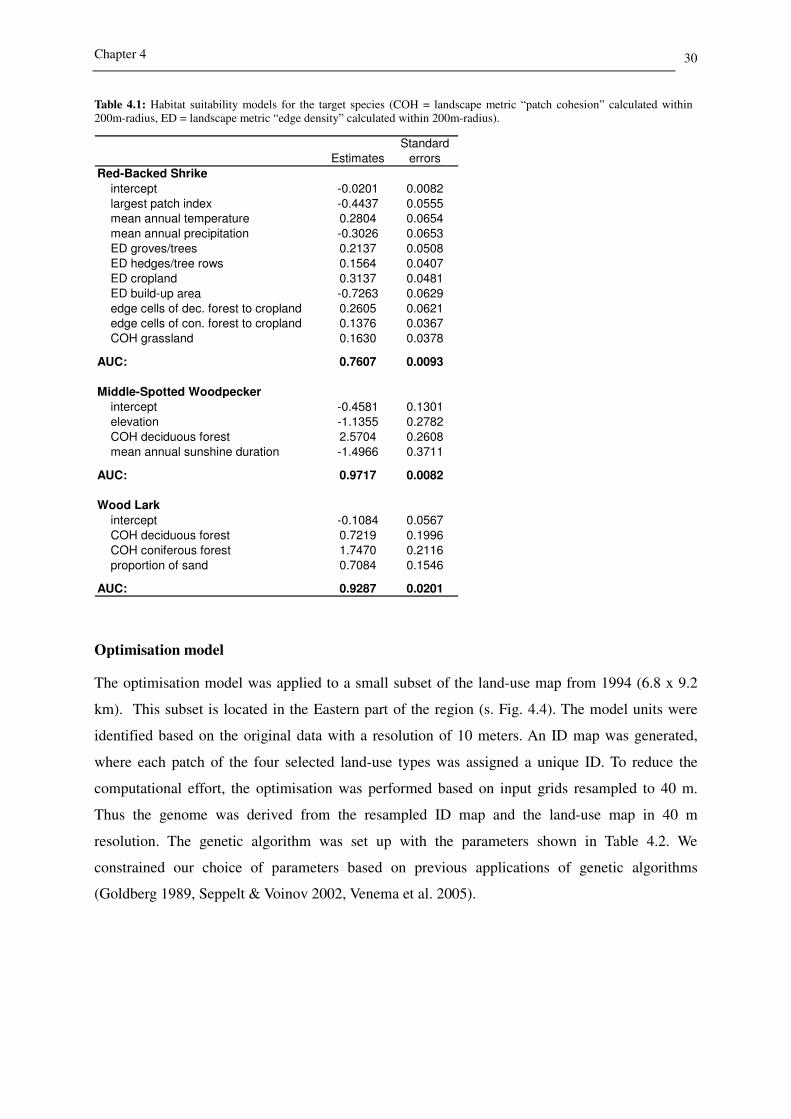
achieved for the Middle-Spotted Woodpecker (AUC: 0.97) (s. Table 4.1). This model includes the

independent variables elevation, mean annual sunshine duration and the patch cohesion of

deciduous forest within the species’ home range. The most important factor is patch cohesion of

deciduous forest. The model fit of the Wood Lark model is also very good (AUC: 0.93). This

model identifies a positive impact of the patch cohesion of coniferous forest and also deciduous

forest within a 200 m radius, but the influence of coniferous forest is much stronger. Furthermore,

the proportion of sand at the specific location has a significant positive effect on habitat suitability

for the Wood Lark. With an AUC of 0.76 the Red-Backed Shrike model is acceptable. It includes

negative effects of the habitat variables largest patch index, mean annual precipitation and edge

density of build-up area. The most important positive factor in this model is the edge density of

cropland, followed by mean annual temperature, number of edge cells of deciduous forest to

cropland, edge density of groves and single trees, patch cohesion of grassland, edge density of

hedges and tree rows and number of edge cells of coniferous forest to cropland. In summary, it

can be ascertained that the Red-Backed Shrike prefers warm and dry conditions in heterogeneous

agricultural landscapes with a high edge density of forest, groves and hedges.

Chapter 4 30

Table 4.1: Habitat suitability models for the target species (COH = landscape metric “patch cohesion” calculated within 200m-radius, ED = landscape metric “edge density” calculated within 200m-radius).

Estimates

Standard

errors

Red-Backed Shrike

intercept -0.0201 0.0082

largest patch index -0.4437 0.0555

mean annual temperature 0.2804 0.0654

mean annual precipitation -0.3026 0.0653

ED groves/trees 0.2137 0.0508

ED hedges/tree rows 0.1564 0.0407

ED cropland 0.3137 0.0481

ED build-up area -0.7263 0.0629

edge cells of dec. forest to cropland 0.2605 0.0621

edge cells of con. forest to cropland 0.1376 0.0367

COH grassland 0.1630 0.0378

AUC: 0.7607 0.0093

Middle-Spotted Woodpecker

intercept -0.4581 0.1301

elevation -1.1355 0.2782

COH deciduous forest 2.5704 0.2608

mean annual sunshine duration -1.4966 0.3711

AUC: 0.9717 0.0082

Wood Lark

intercept -0.1084 0.0567

COH deciduous forest 0.7219 0.1996

COH coniferous forest 1.7470 0.2116

proportion of sand 0.7084 0.1546

AUC: 0.9287 0.0201

Optimisation model

The optimisation model was applied to a small subset of the land-use map from 1994 (6.8 x 9.2

km). This subset is located in the Eastern part of the region (s. Fig. 4.4). The model units were

identified based on the original data with a resolution of 10 meters. An ID map was generated,

where each patch of the four selected land-use types was assigned a unique ID. To reduce the

computational effort, the optimisation was performed based on input grids resampled to 40 m.

Thus the genome was derived from the resampled ID map and the land-use map in 40 m

resolution. The genetic algorithm was set up with the parameters shown in Table 4.2. We

constrained our choice of parameters based on previous applications of genetic algorithms

(Goldberg 1989, Seppelt & Voinov 2002, Venema et al. 2005).

Chapter 4 31

Table 4.2: Parameters of genetic algorithm application (pinit = probability of random disturbance in initial population, pcross = probability of crossover, pmut = probability of mutation, prepl = proportion of population overlap).

population size 10

p init 0.03

p cross 0.6

p mut 0.01

number of generations 1500

p repl [%] 0.25

To analyse how composition and configuration vary with the weightings for the selected species

for which habitat suitability is maximised, we carried out a sensitivity analysis with variable

species’ weightings. The optimisation was performed for all possible combinations of weightings

with increments of 0.1 (66 combinations = possible number of weighting combinations where

weightings add up to one). The resulting optimal landscapes were analysed using a set of

landscape metrics to describe various aspects of land-use pattern and habitat suitability for the

target species. In detail, we used the metrics number of patches (NP), edge density (ED), largest

patch index (LPI), Shannon’s diversity index (SHDI) and contagion index (CONTAG) on

landscape level, and class area (CA) and patch cohesion (COH) of the four changeable land-use

types. In contrast to the metrics used in the habitat suitability models, these metrics were not

calculated by using a moving window analysis. Landscape metrics at landscape level describe

fragmentation (NP and ED), landscape homogeneity (LPI), diversity of land-use types (SHDI) and

aggregation of land-use classes (CONTAG). Class areas of the changeable land-use types show

changes in landscape composition, while patch cohesion also quantifies the connectedness of

these land-use types. For the comparison of the optimisation results with the initial landscape, the

same metrics were used as for the comparisons among the optimisation results. As the species

weights add up to one, the optimisation results can be presented in ternary plots, where the three

axes represent the ratios of species weightings. The plots are read considering the intersections of

the parallels to each of the three axes.

To investigate the effects of landscape configuration separately, constraints were introduced into

the performance criterion to keep landscape composition relatively constant (Equation 4.9). As

model units are of different sizes, it would be difficult to realise changes in configuration while

keeping the initial landscape composition. Thus we allowed a deviation of up to 1 % for each

changeable land-use class (Equation 4.10). With these constraints incorporated, the evolutions of

habitat suitability values were recorded for the three optimisation runs for the three discrete

species and compared to the unconstrained runs.

( )( ) concon fMJJ ⋅= (4.9)

Chapter 4 32

where

M0 = initial state of land-use map

C = total number of cells

cl = number of cells of class l

l = land-use type∈ Lg

If all species were equally weighted, the improvement would be towards the optimum for the

species with the highest sensitivity to changes in the genetic algorithm, and genes that could

improve habitat suitability for other species might get lost. To enhance habitat suitability for all

three target species in equal measure, we need to weight the species according to their sensitivity

to land-use changes. Thus, habitat suitability values derived from the optimised landscapes were

normalised for each species by division through the maximum habitat suitability. The maximum

sum of normalised habitat suitabilities for the three species was determined and the species’

weightings were derived accordingly.

4.4 Results

Do species habitat requirements contrast or coincide?

Habitat suitabilities (HSI) for all three target species improved during almost all optimisation

runs, except for the runs optimising habitat suitability for the Wood Lark and the Middle-Spotted

Woodpecker, where Red-Backed Shrike habitat suitability decreased. We also observed a slight

decrease of habitat suitability for Wood Lark in the runs optimising habitat suitability for Middle-

Spotted Woodpecker and Red-Backed Shrike (Fig. 4.5). The highest mean habitat suitability

values were reached for the Middle-Spotted Woodpecker (mean HSI between 0.52 and 0.95). In

almost all optimisation runs, mean HSI for the Middle-Spotted Woodpecker exceeded those of the

other species. The optimisation was least successful for the Red-Backed Shrike (mean HSI

between 0.30 and 0.54). For the Wood Lark, the mean habitat suitability varies between 0.28 and

0.74. As the initial mean habitat suitability index was 0.40 for the Middle-Spotted Woodpecker,

0.30 for the Wood Lark and 0.32 for the Red-Backed Shrike, the improvement was best for the

Middle-Spotted Woodpecker and worst for the Red-Backed Shrike. The minimum values of

habitat suitability of the Middle-Spotted Woodpecker and the Wood Lark are reached when the

weight for Red-Backed Shrike is high (0.9). Before that habitat suitabilities for the Middle-

1 if ( ) ( )( )gMcMcC

ll −0

1 < 0.01 for l = 1,2,3,4

=conf

0 else

(4.10)

Chapter 4 33

Figure 4.5: Mean habitat suitability indices (HSI) of the target species (MSW = Middle-Spotted Woodpecker, WL = Wood Lark, RBS = Red-Backed Shrike) depending on species’ weightings (w_MSW = weight for Middle-Spotted Woodpecker, w_WL = weight for Wood Lark, w_RBS = weight for Red-Backed Shrike); white dots indicate maximum values; black dots indicate minimum values; lines indicate mean HSI values derived from the initial landscape; for MSW the initial value is below the values in the plot.

Spotted Woodpecker and the Wood Lark decrease more slightly when the weight for Red-Backed

Shrike is increased. The lowest values of the Red-Backed Shrike habitat suitability are found

when the weight for the Wood Lark is highest.

How do landscape composition and configuration differ in landscapes optimised for each of

the three target species?

Figure 4.6 shows the effects of species weightings on landscape configuration at the landscape

level. Landscapes optimised for the Middle-Spotted Woodpecker show the most homogenous and

least diverse pattern. The Red-Backed Shrike prefers the most diverse and fragmented landscapes,

while landscapes optimised for the Wood Lark are intermediate. Landscape homogeneity was

much higher in the initial landscape than in those optimised for the Red-Backed Shrike and the

Wood Lark, but lower than in the landscape optimised for the Middle-Spotted Woodpecker. The

contagion index is lower in the initial landscape than in those optimised for the Middle-Spotted

Woodpecker and the Wood Lark, but it is slightly higher than in the landscape optimised for the

Red-Backed Shrike. Likewise, landscape diversity is higher in the landscape optimised for the

Red-Backed Shrike than in the initial landscape and much lower in the landscapes optimised for

Wood Lark and Middle-Spotted Woodpecker.

Chapter 4 34

Figure 4.6: Landscape metrics largest patch index (LPI), contagion index (CONTAG) and Shannon diversity index (SHDI) on landscape level depending on species’ weightings (w_MSW = weight for Middle-Spotted Woodpecker, w_WL = weight for Wood Lark, w_RBS = weight for Red-Backed Shrike); white dots indicate maximum values; black dots indicate minimum values; lines indicate values of initial landscape. The metric largest patch index (LPI) equals the percent of the landscape that the largest patch comprises. The contagion index (CONTAG) shows the aggregation of land-use classes in the landscape and the Shannon diversity index (SHDI) indicates the diversity of patch types in the landscape.

Results of the analysis of landscape composition depending on the combination of species’

weightings correspond to the habitat suitability models, but they also show the effects of

contrasting habitat requirements. The Middle-Spotted Woodpecker prefers deciduous forest, the

Wood Lark prefers coniferous forest and the Red-Backed Shrike favours cropland and grassland

(Fig. 4.7). The proportion of cropland is lowest in the runs optimised for the Wood Lark. This

indicates that the Wood Lark avoids cropland more than the Middle-Spotted Woodpecker does,

which explains why the habitat requirements of the Red-Backed Shrike contrast more sharply

with those of the Wood Lark than those of the Middle-Spotted Woodpecker (see Figure 4.5). The

contrast in habitat requirements of Middle-Spotted Woodpecker can be explained by the

proportion of deciduous forest. To a certain extent, the Red-Backed Shrike is more tolerant to the

proportion of deciduous forest than the Wood Lark, but when the weight for the Red-Backed

Shrike exceeds 0.6, deciduous forest is increasingly avoided.

The Wood Lark avoids grass- and cropland and to a certain extent also deciduous forest, but

habitat suitability for the Wood Lark is not well-characterised by the proportion of coniferous

forest alone. Deciduous forest also has a positive effect, but the positive effect of coniferous forest

is higher (Table 4.1).

When we compare the initial landscape composition to those of the optimisation results, we see

that the proportion of cropland has decreased during all optimisation runs. Also, the proportion of

grassland decreased compared to the initial landscape, except for the optimisation with respect to

the Red-Backed Shrike, where an increase occurred. Compared to the initial landscape, the

proportion of deciduous forest is higher in all optimisation runs. The proportion of coniferous

forest has increased in the optimisations for the Wood Lark and decreased in those for the Middle-

Spotted Woodpecker and the Red-Backed Shrike.

Chapter 4 35

Figure 4.7: Area of the four changeable classes depending on species’ weightings (w_MSW = weight for Middle-Spotted Woodpecker, w_WL = weight for Wood Lark, w_RBS = weight for Red-Backed Shrike); white dots indicate maximum values; black dots indicate minimum values; lines indicate values of initial landscape.

How do landscape composition and configuration contribute to an improvement of habitat

suitability?

Figure 4.8 shows the dependence of the evolution of the mean habitat suitability on the

optimisation criterion for all three target species. By maximising habitat suitability for the Middle-

Spotted Woodpecker, the habitat suitabilities for the Wood Lark and the Red-Backed Shrike are

also slightly increased initially, but after about 800 evaluations they decrease and, in the end,

habitat suitability for the Red-Backed Shrike falls below the initial value. The increase in habitat

suitability for the Wood Lark within the first 800 evaluations is due to an increase in deciduous

forest. Thereafter, habitat suitability for the Wood Lark decreases as the proportion of coniferous

forest decreases in favour of the proportion of deciduous forest.

Chapter 4 36

Figure 4.8: Dependence of the evolution of mean habitat suitability for target species and the proportions of changeable land-use types on the optimisation criterion (MSW_opt = maximise habitat suitability for MSW, WL_opt = maximise habitat suitability for WL, RBS_opt = maximise habitat suitability for RBS).

Maximising habitat suitability for the Wood Lark slightly decreases habitat suitability for the Red-

Backed Shrike after the first 250 evaluations and leads to an unsteady increase in habitat

suitability for the Middle-Spotted Woodpecker.

Optimising for the Red-Backed Shrike also increases habitat suitability for the Middle-Spotted

Woodpecker, which achieves even higher mean habitat suitability values by the end of the

Chapter 4 37

optimisation. Mean habitat suitability for the Wood Lark increases within the first 200

evaluations, but slightly decreases afterwards until it finally reaches its initial value.

When we compare the evolution of habitat suitabilities to the proportions of changeable land-use

types, we see that changes in habitat suitability for the Middle-Spotted Woodpecker are essentially

driven by the proportion of deciduous forest. Changes in habitat suitability for the Wood Lark are

mainly driven by the proportion of coniferous forest and, to a certain extent, by changes in the

proportion of deciduous forest. The changes in habitat suitability for the Red-Backed Shrike are

not driven by single land-use types. The Red-Backed Shrike benefits from a decrease of cropland

to about 40% in favour of an increase of deciduous forest (Fig. 4.8). It is striking that within the

first evaluations habitat suitabilities are increased in all optimisation runs.

To investigate the effects of landscape configuration, the optimisation was performed for all three

species while keeping landscape composition constant. The results of the constrained

optimisation, shown in Figure 4.9 and Table 4.3, indicate that the possibilities for an improvement

of habitat suitability are limited when only changes in landscape configuration are allowed. The

best improvement is achieved for the Red-Backed Shrike, the worst for the Wood Lark. However,

there seem to be no considerable contrasts between the species’ habitat requirements with respect

to landscape configuration (Figure 4.9). The optimisations for the Middle-Spotted Woodpecker

and the Wood Lark increase habitat suitabilities for all three species, but changes in habitat

suitability for the Red-Backed Shrike have hardly any effect on habitat suitabilities for the other

two species. Habitat configuration requirements of the Red-Backed Shrike differ from those of the

other two species. For this species, the improvement of habitat suitability through changes in

landscape configuration was almost as good as through changes in landscape composition and

configuration. The landscape configuration optimised for the Red-Backed Shrike is the most

heterogeneous (highest number of patches and edge density, lowest largest patch index value on

the landscape level) as connectivities (patch cohesion) of cropland, deciduous forest and

coniferous forest are the lowest (Table 4.3). The optimisation for the Middle-Spotted Woodpecker

led to the most homogeneous land-use pattern (highest largest patch index and number of patches,

lowest edge density on landscape level). In this run, patch cohesion of deciduous forest is higher

than in the runs optimised for the Wood Lark and the Red-Backed Shrike. Likewise, patch

cohesion of coniferous forest is highest in the run optimised for the Wood Lark. However, in the

initial landscape, values of both patch cohesion of deciduous and coniferous forest are higher.

This can be explained by the fact that the habitat variables “patch cohesion of

deciduous/coniferous forest” are calculated within the species’ home ranges, whereas for the

comparison of optimisation results the same metrics were calculated for the whole landscape

subset.

Chapter 4 38

Figure 4.9: Dependence of the evolution of mean habitat suitabilities for target species with constant landscape composition depending on the optimisation criterion (MSW_opt = maximise habitat suitability for MSW, WL_opt = maximise habitat suitability for WL, RBS_opt = maximise habitat suitability for RBS).

What characterises a landscape optimised for all three target species?

The sums of the normalised mean habitat suitabilities for all species are shown in Figure 4.10. The

white dot indicates the maximum of the normalised mean habitat suitabilities, which is reached

with species’ weightings of 0.23 (Middle-Spotted Woodpecker), 0.32 (Wood Lark) and 0.45 (Red-

Backed Shrike).

Chapter 4 39

Figure 4.10: Sums of normalised mean habitat suitabilities (HSI) of target species depending on species’ weightings; white dot shows maximum sum.

Figure 4.11 shows the landscape pattern optimised for all three species according to the species’

weightings derived from Figure 4.10. Compared to the initial landscape, the optimisation result is

characterised by a lower proportion of grassland and cropland and a higher proportion of

deciduous and coniferous forest (Fig. 4.11, Table 4.3). Landscape configuration is less compact

and aggregated and the pattern is slightly more diverse in the optimised landscape (Fig. 4.11,

Table 4.3). Cropland is concentrated in the South-Western part of the landscape subset, where

model units are small. Larger model units are occupied by deciduous or coniferous forest. Mean

habitat suitability for the Middle-Spotted Woodpecker and the Wood Lark increased by 0.36. The

increase in mean habitat suitability for the Red-Backed Shrike was only 0.12.

Figure 4.11: Initial landscape (a) and result (b) of optimisation for all three target species according to species’ weightings 0.23 (MSW), 0.32 (WL) and 0.45 (RBS).

Chapter 4 40

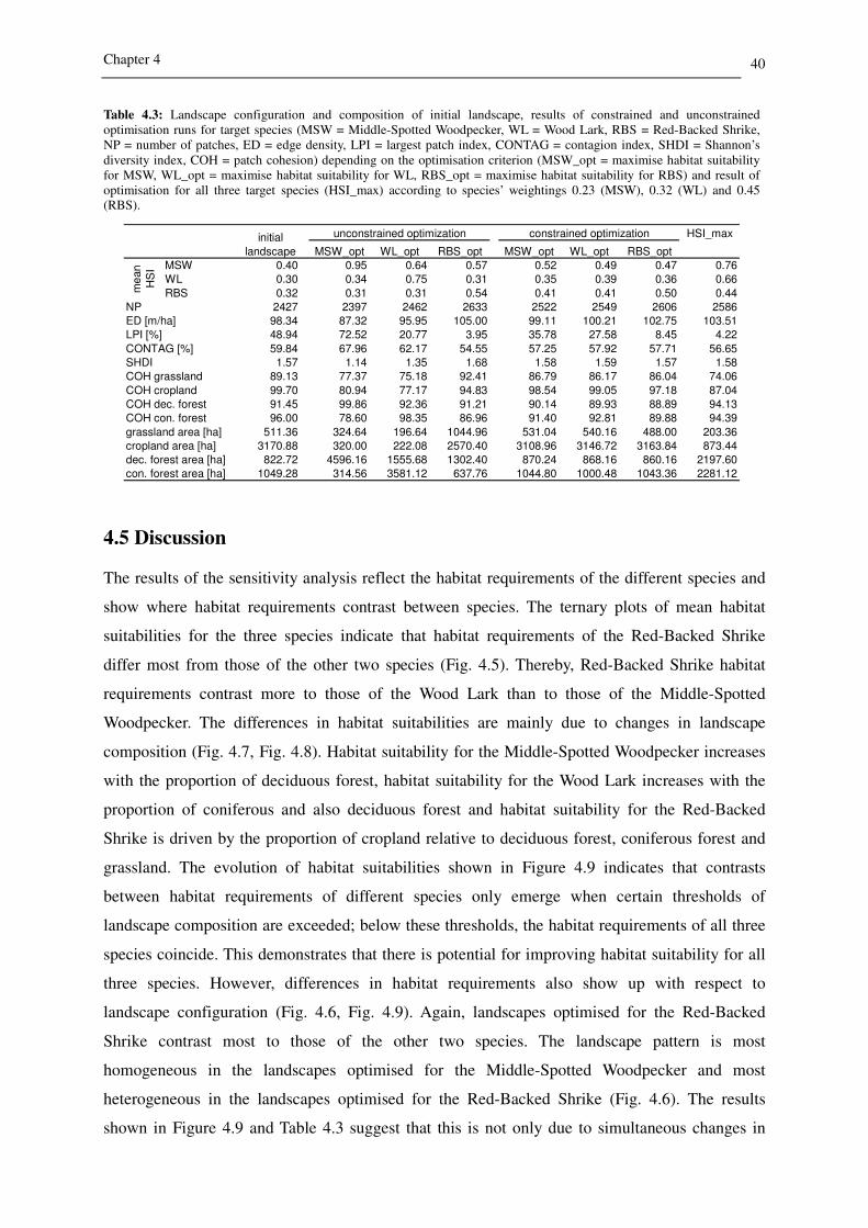
Table 4.3: Landscape configuration and composition of initial landscape, results of constrained and unconstrained optimisation runs for target species (MSW = Middle-Spotted Woodpecker, WL = Wood Lark, RBS = Red-Backed Shrike, NP = number of patches, ED = edge density, LPI = largest patch index, CONTAG = contagion index, SHDI = Shannon’s diversity index, COH = patch cohesion) depending on the optimisation criterion (MSW_opt = maximise habitat suitability for MSW, WL_opt = maximise habitat suitability for WL, RBS_opt = maximise habitat suitability for RBS) and result of optimisation for all three target species (HSI_max) according to species’ weightings 0.23 (MSW), 0.32 (WL) and 0.45 (RBS).

HSI_max

MSW_opt WL_opt RBS_opt MSW_opt WL_opt RBS_opt

MSW 0.40 0.95 0.64 0.57 0.52 0.49 0.47 0.76

WL 0.30 0.34 0.75 0.31 0.35 0.39 0.36 0.66

RBS 0.32 0.31 0.31 0.54 0.41 0.41 0.50 0.44

2427 2397 2462 2633 2522 2549 2606 2586

98.34 87.32 95.95 105.00 99.11 100.21 102.75 103.51

48.94 72.52 20.77 3.95 35.78 27.58 8.45 4.22

59.84 67.96 62.17 54.55 57.25 57.92 57.71 56.65

1.57 1.14 1.35 1.68 1.58 1.59 1.57 1.58

89.13 77.37 75.18 92.41 86.79 86.17 86.04 74.06

99.70 80.94 77.17 94.83 98.54 99.05 97.18 87.04

91.45 99.86 92.36 91.21 90.14 89.93 88.89 94.13

96.00 78.60 98.35 86.96 91.40 92.81 89.88 94.39

511.36 324.64 196.64 1044.96 531.04 540.16 488.00 203.36

3170.88 320.00 222.08 2570.40 3108.96 3146.72 3163.84 873.44

822.72 4596.16 1555.68 1302.40 870.24 868.16 860.16 2197.60

1049.28 314.56 3581.12 637.76 1044.80 1000.48 1043.36 2281.12

NP

ED [m/ha]

LPI [%]

CONTAG [%]

SHDI

grassland area [ha]

cropland area [ha]

dec. forest area [ha]

con. forest area [ha]

COH grassland

COH cropland

COH dec. forest

COH con. forest

initial

landscape

unconstrained optimization constrained optimization

me

an

HS

I

4.5 Discussion

The results of the sensitivity analysis reflect the habitat requirements of the different species and

show where habitat requirements contrast between species. The ternary plots of mean habitat

suitabilities for the three species indicate that habitat requirements of the Red-Backed Shrike

differ most from those of the other two species (Fig. 4.5). Thereby, Red-Backed Shrike habitat

requirements contrast more to those of the Wood Lark than to those of the Middle-Spotted

Woodpecker. The differences in habitat suitabilities are mainly due to changes in landscape

composition (Fig. 4.7, Fig. 4.8). Habitat suitability for the Middle-Spotted Woodpecker increases

with the proportion of deciduous forest, habitat suitability for the Wood Lark increases with the

proportion of coniferous and also deciduous forest and habitat suitability for the Red-Backed

Shrike is driven by the proportion of cropland relative to deciduous forest, coniferous forest and

grassland. The evolution of habitat suitabilities shown in Figure 4.9 indicates that contrasts

between habitat requirements of different species only emerge when certain thresholds of

landscape composition are exceeded; below these thresholds, the habitat requirements of all three

species coincide. This demonstrates that there is potential for improving habitat suitability for all

three species. However, differences in habitat requirements also show up with respect to

landscape configuration (Fig. 4.6, Fig. 4.9). Again, landscapes optimised for the Red-Backed

Shrike contrast most to those of the other two species. The landscape pattern is most

homogeneous in the landscapes optimised for the Middle-Spotted Woodpecker and most

heterogeneous in the landscapes optimised for the Red-Backed Shrike (Fig. 4.6). The results

shown in Figure 4.9 and Table 4.3 suggest that this is not only due to simultaneous changes in

Chapter 4 41

landscape composition, where landscape homogeneity is increased with the proportion of a certain

land-use type, but also to changes in landscape configuration. The improvement of habitat

suitability for the Middle-Spotted Woodpecker and the Wood Lark is low when landscape

composition is kept constant. Habitat requirements of the Wood Lark and the Middle-Spotted

Woodpecker coincide with respect to landscape configuration. This might be due to the fact that

the configuration of deciduous forest is important for both species. For the Red-Backed Shrike,

changes in landscape configuration alone can improve habitat suitability almost as much as

changes in landscape composition and configuration. This reflects Red-Backed Shrike’s strong

dependence on complex habitat structures. The fact that the habitat suitability for the Middle-

Spotted Woodpecker is highest in all runs with a non-zero weighting for the Middle-Spotted

Woodpecker can be explained by the high sensitivity of this habitat model towards alternations in

the genetic algorithm. The most important reason for the high sensitivity towards the genetic

algorithm is the simplicity of the habitat model. Patch cohesion of deciduous forest is the only

habitat variable that can be influenced and has the highest model coefficient. Thus, changes in the

genetic algorithm cause great changes in habitat suitability and therefore habitat suitability can be

improved to a greater extent. The Wood Lark model contains two variables that can be influenced.

As in the Middle-Spotted Woodpecker model, these variables are the ones with the highest

coefficients, but still the sensitivity of the Wood Lark habitat model is lower. This can be

explained by the fact that an increase in two land-use types is needed instead of just one in the

Middle-Spotted Woodpecker model. The model with the most variables is the Red-Backed Shrike

model, thus it shows the lowest sensitivity towards changes in the genetic algorithm. Additionally,

the most important factor is the edge density of build-up area within the species’ home range,

which is not a modifiable variable. The influences of the changeable variables (edge density of

cropland, edge cells of deciduous and coniferous forest to cropland and patch cohesion of

grassland) are comparatively low and, thus, the algorithm converges at a much lower level. These

findings need to be taken into account when optimising landscape configuration with respect to all

three target species. If all species were equally weighted, the optimisation would favour the

Middle-Spotted Woodpecker more than the other two species because Middle-Spotted

Woodpecker is most sensitive to the modelled changes and, therefore, genes that could improve

habitat suitability for other species could get lost. Therefore, the mean habitat suitabilities of all

runs were normalised and summed up to find the weighting combination where the best trade-off

between all species can be achieved (Fig. 4.10). At this ideal trade-off point, the highest weight is

given to the Red-Backed Shrike – the species with the lowest sensitivity towards changes in the

genetic algorithm – and the lowest to Middle-Spotted Woodpecker, which is most sensitive. The

comparison of the initial landscape to the landscape optimised for all three species showed that an

increase in deciduous and coniferous forest and a decrease of crop- and grassland could improve

Chapter 4 42

habitat suitability for all three species. Furthermore, all species benefit from an increase in

landscape heterogeneity, landscape diversity and a disaggregation of land-use classes (Fig. 4.11,

Table 4.3). Still, the increase in habitat suitability for the Red-Backed Shrike is smaller than for

the two other species. This indicates that other management actions need to be taken into

consideration to improve habitat suitability for this species.

4.6 Conclusions

The approach outlined in this paper shows promise as a tool for analysing the effects of land-use

changes on different species and for detecting conflicts between species.

We investigated the effects of different land-use changes on habitat suitability for three target

species. An increase of deciduous and coniferous forest and a decrease of cropland and grassland

in the landscape subset have positive effects on all target species. Middle-Spotted Woodpecker

habitat suitability depends mainly on the proportion of deciduous forest. An increase of coniferous

forest has a positive effect on habitat suitability for the Wood Lark, whereas for the Red-Backed

Shrike juxtaposing patches of cropland, groves and deciduous forest is optimal. This species is

highly depended on landscape configuration and its habitat requirements contrast most with those

of the other two target species. However, land-use changes between cropland, grassland,

deciduous and coniferous forest do not allow an improvement of habitat suitabilities for all three

model species in equal measure.

The methodology presented and applied in this study could be a useful tool to support

conservation management decisions, even though there are some clear improvement

opportunities. The optimisation approach is very flexible and could easily incorporate other

spatially-referenced conservation objectives. It can detect trade-offs between different

management objectives and identify the solution space where all objectives are improved. In a

conservation application, species’ weightings could be assigned according to conservation status.

Using patch topology within the optimisation produced reasonable land-use patterns, as the units

of change correspond to the land-use parcels on which decisions are made. However, at this point

the approach could be improved by incorporating linear land-use changes like the introduction of

hedges along field edges. This could be interesting when considering functions or processes that

are affected by linear landscape elements (e.g. Red-Backed Shrike habitat suitability, erosion). As

the model results of this case study are not realistic, further constraints need to be considered to

enhance usability for conservation planning. Thus, we plan to include economic considerations

into the performance criterion to take into account cost effectiveness of land-use changes in a

future study.

Chapter 4 43

Acknowledgements

We would like to thank Dr. Carsten Dormann for support in statistical modelling and comments

on the manuscript and we thank Michael Müller for his technical support, his C++ routine for

deriving ID maps from a categorical map and the possibility to use the computer cluster of the

Department of Ecological Modelling, UFZ Leipzig-Halle. The software package R (R

Development Core Team 2005) was used for model calculations.