DISTANCE AND SPEED MEASUREMENT TECHNIQUES

P.Abdul Nazer “Simulation of overtaking manoeuvres in mixed traffic environment”, Department of Civil Engineering,Regional Engineering CollegeCalicut , University of Calicut, 2002

CHAPTER - 3 DISTANCE AND SPEED MEASUREMENT TECHNIQUES

Today, with the advent of modern computers and the development in the

instrumentation industry, sophisticated equipments are readily available in the market

to collect any type of traffic data from the road. It has the power to observe, store

and analyse or even to print the results of the field observations. Certain studies like

the study of overtaking behaviour, needs spatial data like the speed, the acceleration,

the lateral and the longitudinal positions of vehicles on the entire stretch of overtaking

zone. The spatial observation systems are very costly. Those are not affordable for

studies which are of academic interest. Two simple and least expensive techniques

for traffic data collection have been developed and briefly presented in this chapter.

Many of the Traffic Engineering studies specifically related to hypotheses

formulation and testing of theories of traffic flow, vehicular overtaking behavioural

studies and development of safe passing sight distance, etc, need spatial data. The

first part of this chapter describes, a procedure developed for vehicular detection and

computerised data retrieval for traction of vehicles in mid blocks using moving camera

method.

An accurate and automatic speed recording system is presented in the second

l part. It is a direct reading mechanism using a computer, based on the signals received

from the two probes placed at a fixed distance apart on the highway section. l

3.2 TRACING THE PATH FOLLOWED BY VEHICLES IN MIDBLOCKS

i USING MOVING CAMERA METHOD

l 3.2.1 INTRODUCTION

l Many instrumental methods have been developed for the collection of

data like the speeds of vehicles, the traffic volumes, the head ways, etc., all at chosen

locations. Since all those measurements are location specific, they can hardly be used

to study the vehicle acceleration and deceleration characteristics, like the linear and

the lateral positioning of vehicles. There is a need for development of simple methods

for tracing the path followed by vehicles in relation to time over a space or stretch

of roadway. A simple technique has been developed for achieving this objective.

However, it is felt that the fuller utility of the proposed technique could be realised

only when the image processing techniques are possible to be coupled with the method

developed in this study.

3.2.2 PRINCIPLE USED IN THE CALCULATION OF

DISTANCE USING IMAGE SIZE

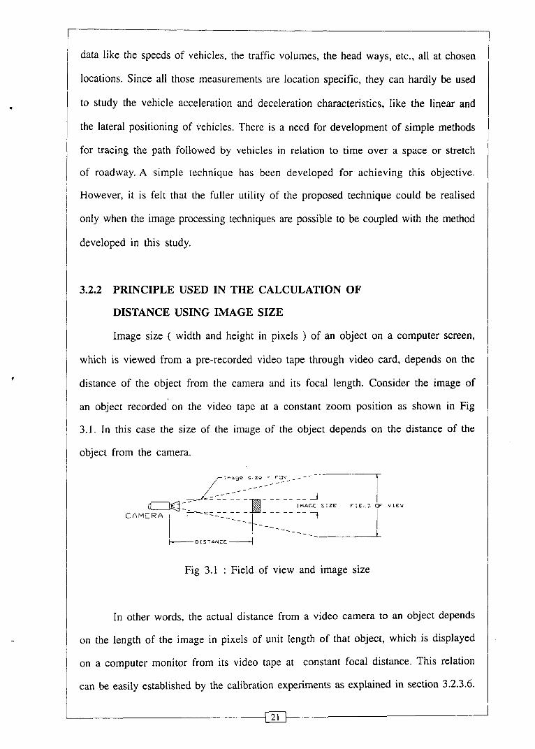
Image size ( width and height in pixels ) of an object on a computer screen,

which is viewed from a pre-recorded video tape through video card, depends on the

distance of the object from the camera and its focal length. Consider the image of

an object recorded'on the video tape at a constant zoom position as shown in Fig

3.1. In this case the size of the image of the object depends on the distance of the

object from the camera.

d C A M E R A

I n a g e s , z e = T K I V - - , - -

_ C / - - - _----- -7 I M A G E S I Z E F I E L O O F

- ---- - - --I------- - - -

1- D I STANCE -1

Fig 3.1 : Field of view and image size

In other words, the actual distance from a video camera to an object depends

on the length of the image in pixels of unit length of that object, which is displayed

on a computer monitor from its video tape at constant focal distance. This relation

can be easily established by the calibration experiments as explained in section 3.2.3.6.

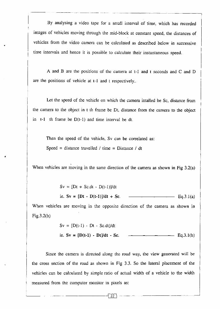
By analysing a video tape for a small interval of time, which has recorded

images of vehicles moving through the mid-block at constant speed, the distances of

vehicles from the video camera can be calculated as described below in successive

time intervals and hence it is possible to calculate their instantaneous speed.

A and B are the positions of the camera at t-l and t seconds and C and D

are the positions of vehicle at t-l and t respectively..

Let the speed of the vehicle on which the camera intalled be Sc, distance from I the camera to the object in t th frame be Dt, distance from the camera to the object

in t-l th frame be D(t-l) and time interval be dt.

Then the speed of the vehicle, Sv can be correlated as:

Speed = distance travelled I time = Distance / dt

When vehicles are moving in the same direction of the camera as shown in Fig 3.2(a)

SV = [Dt + Sc.dt - D(t-l)]/dt

ie. Sv = [Dt - D(t-l)]/dt + Sc. Eq.3. l (a)

When vehicles are moving in the opposite direction of the camera as shown in

Fig.3.2(b)

SV = [D((-l) - Dt - Sc.dt]/dt

ie. Sv = [D(t-l) - Dt]/dt - Sc. Eq.3.l(b)

l Since the camera is directed along the road way, the view generated will be

the cross section of the road as shown in Fig 3.3. So the lateral placement of the

/ vehicles can be calculated by simple ratio of actual width of a vehicle to the width I

measured from the computer monitor in pixels as:

Distance

l !

1- <Sc.dt> D I

Fig.3.2(b)Positions of vehicle and camera at t and t-l seconds moving in the opposite

directions.

Fig.3.2(a):Positions of vehicle and camera at t and t-l seconds moving in the same

L / I = W / w = R / r Eq. 3.2.

direction - D( [ - I )

- - -- - j A K - - - - - r ~ l<- -- - 4 4 - ~

J

<Sc.dr> D I

Where :

L - actual left clearance , I

1 - measured left clearance

R - actual right clearance

r - measured right clearance

W - actual width of vehicle

W - measured width of vehicle

l Fig 3.3 : Cross sectional view of the road

- D ~ s t a n c e

-

- l- - - <

1- - -J c F--

l 1 Therefore : i

R = ( W / w ) x r Eq.3.4

But ( W / W ) is the width factor (K).

i e . L = K x l Eq.3.5

R = K x r Eq.3.6

Width factor K varies with the distance from the camera.

3.2.3 CALIBRATION OF VIDEO CAMERA

The calibration of a video camera is performed to find out the relation

1 between the distance from the camera to an object and the width factor. Width factor

/ (K) is defined as the ratio of actual size ( in any direction ) of an object in metres ! i and its corresponding size measured from the computer monitor in pixels. 1

3.2.3.1 IDENTIFICATION OF THE VIDEO CAMERA AND ZOOM

In this study, calibration experiments were conducted on Panasonic M 900

camera in which the different zooms are shown in the display as 1, 2, 3, etc.

i

camera.

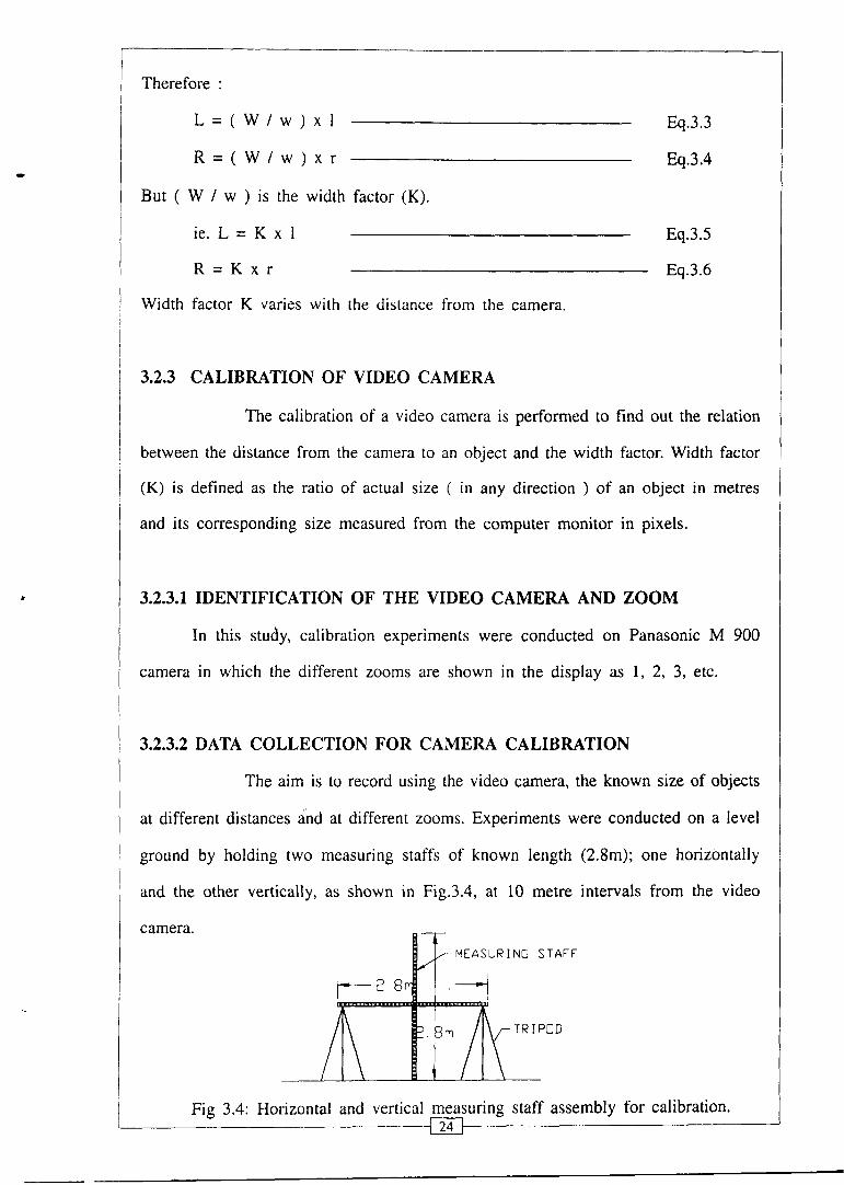
' 3.2.3.2 DATA COLLECTION FOR CAMERA CALIBRATION

The aim is to record using the video camera, the known size of objects l / at different distances and at different zooms. Experiments were conducted on a level

l I ground by holding two measuring staffs of known length (2.8m); one horizontally

and the other vertically, as shown in Fig.3.4, at 10 metre intervals from the video

STAFF

!

I POD

-

1 Fig 3.4: Horizontal and vertical measuring staff assembly for calibration. - p r J

r- V E R T I C A L S T A F F

r C A M E R A

l Fig 3.5: Camera and measuring staff setup.

I I

The view of the staff set up was recorded for about 2 seconds by setting the

zoom to 1 and this was repeated for various distances of 20m, 30m, etc,. up to 80m,

as shown in Fig.3.5. These experiments were repeated for all other possible zooms

of 2, 3 and 4 for the video camera selected. Here in this study 4 zooms were selected

for Panasonic M900 video camera.

-HORIZONTAL S T A F F

TRIPOD I

3.2.3.3 DATA RETRIEVAL SYSTEM

OM I

10 I

2 0 I

30 I

4 0 5 0 6 0 70 8 0

For the retrieval of the recorded data a powerful PC with frame grabber

or a video card is necessary. V.C.R or a video camera can be connected directly to

this card. Required software to display the video tape and to record the current screen

are to be installed in the PC ( Imagescan and HyperCam are used in this study ).

The data retrieval system is shown schematically in Fig.3.6.

r C P U WITH FRAME G R A B B E R

r V I D E O CAMERA

Fig 3.6: Data retrieval system

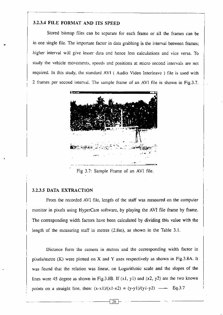
3.2.3.4 FILE FORMAT AND ITS SPEED l Stored bitmap files can be separate for each frame or all the frames can be

in one single file. The important factor in data grabbing is the interval between frames;

higher interval will give lesser data and hence less calculations and vice versa. To

study the vehicle movements, speeds and positions at micro second intervals are not

required. In this study, the standard AV1 ( Audio Video Interleave ) file is used with

2 frames per second interval. The sample frame of an AV1 file is shown in Fig.3.7.

.. .&. - - -- - -. - - - .- -. --- - --

Fig 3.7: Sample Frame of an AV1 file.

3.2.3.5 DATA EXTRACTION

From the recorded AV1 file, length of the staff was measured on the computer

monitor in pixels using HyperCam software, by playing the AV1 file frame by frame.

The corresponding width factors have been calculated by dividing this value with the

length of the measuring staff in metres (2.8m), as shown in the Table 3.1.

Distance form the camera in metres and the corresponding width factor in

pixeldmetre (K) were plotted on X and Y axes respectively as shown in Fig.3.8A. It

was found that the relation was linear, on Logarithmic scale and the slopes of the I lines were 45 degree as shown in Fig.3.8B. If (xl , y l ) and (x2, y2) are the two known

points on a straight line, then: (X-xl)/(xl-x2) = (y-yl)/(yl-y2) - Eq.3.7

Table 3.1: Width factors at different distances for different zooms.

Let the y-intercept at X = 10 be equal to C. Then (10,C) and (C,10) are the

two known points on the line. Therefore:

(Io~(x)-log 1 O)/(log 10-10g(C)) = (l~g(y)-l~g(C))/(l~g(C)-log 10) Eq.3.8

log(x)-log l 0 '= log(C)-log(y) Eq.3.9

log(x) + log(y) = log(C) + log10 Eq.3.10

Camera : Panasonic M900. Length of staff ( 2.8 m )

x.y = 1OC Eq.3.11

X = 1OC/y Eq.3.12

ie. D = 1OCIK Eq.3.13

Distance from

the camera(m)

10

20

3 0

40

50

60

70

80

0 W 20 00 4000 60 00 $0 00

Distance lrom the camera (D) in m

A) Linear scale

Zoom=l

10 00 l00 W 1000 00

Distance lrom the camera (D) In m

Pixel

219

107.5

73

54

43

36

30

27

l00000 --.

E . V) aso- . - m X .- n E .- - 110-

10000- L

0 - 1 0 0 m - 5 P 3

10 00

B) Logarithmic scale

Pixellm

78.21

38.39

26.07

19.28

15.36

12.86

10.71

9.64

Zoom=:!

a - ' .

_i\ zoom =4 ZOO^=^ zoom = 2 zoom = l

T' I I

Fig 3.8. Relation between the distance from the camera and the width factor m

Pixel

327.5

165

110

83

65

54

46

40

Pixellm

116.96

58.93

39.29

29.64

23.2 1

19.29

16.43

14.29

Zoom=3

Pixel

530

273

182

134.5

108

87

77

67 ---

Z O O ~ = ~

PixeUn-

189.29

97.5

65

47.86

38.57

31.07

27.5

23.93

Pixel

-

375.5

251.5

189

147

122

104

-

PixeUm

34.11

89.82

67.5

52.5

43.57

37.14

-

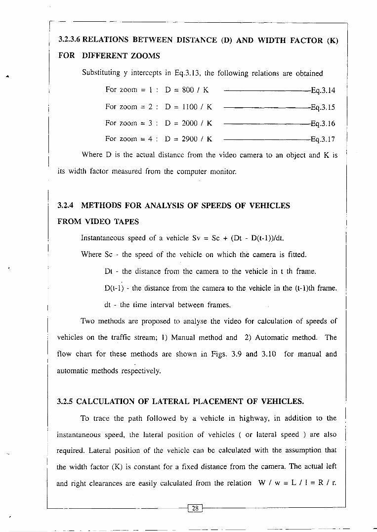
3.2.3.6 RELATIONS BETWEEN DISTANCE (D) AND WIDTH FACTOR (K)

1 FOR DIFFERENT ZOOMS l

Substituting y intercepts in Eq.3.13, the following relations are obtained

For zoom = 1 : D = 800 / K Eq.3.14

For zoom = 2 : D = 11001 K Eq.3.15

For zoom = 3 : D = 2000 / K Eq.3.16

For zoom = 4 : D = 2900 1 K Eq.3.17

Where D is the actual distance froin the video camera to an object and K is

its width factor measured from the computer monitor.

3.2.4 METHODS FOR ANALYSIS OF SPEEDS OF VEHICLES

FROM VIDEO TAPES

Instantaneous speed of a vehicle Sv = Sc + (Dt - D(t-l))/dt.

Where Sc - the speed of the vehicle on which the camera is fitted.

Dt - the distance from the camera to the vehicle in t th frame.

~ ( t - l j - the distance from the camera to the vehicle in the (t-1)th frame.

dt - the time interval between frames.

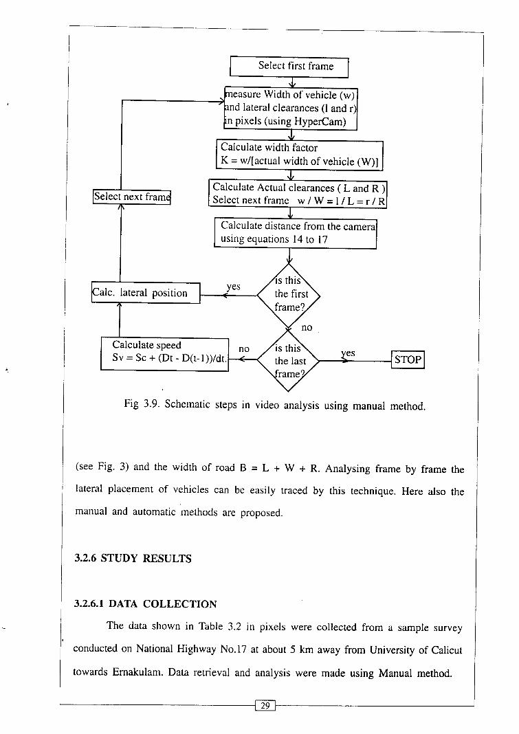
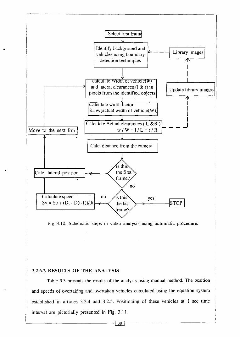
Two methods are proposed to analyse the video for calculation of speeds of

vehicles on the traffic stream; 1) Manual method and 2) Automatic method. The

flow chart for these methods are shown in Figs. 3.9 and 3.10 for manual and

automatic methods respectively. I

3.2.5 CALCULATION OF LATERAL PLACEMENT OF VEHICLES.

To trace the path followed by a vehicle in highway, in addition to the

instantaneous speed, the lateral position of vehicles ( or lateral speed ) are also

required. Lateral position of the vehicle can be calculated with the assumption that

the width factor (K) is constant for a fixed distance from the camera. The actual left

and right clearances are easily calculated from the relation W / W = L / 1 = R 1 r.

Select first frame

, $easure Width of v e h i c l e 1

I 'Fnd lateral clearances (1 and r)(

Select next fram L 5

In pixels (using Hypeream) 1 I

\L I Calculate Actual clearances ( L and R )I I Select next frame W I W = l I L = r / RI

I

Calculate distance from the camera using equations 14 to 17 I Yes .

Calculate speed no SV = Sc + (Dt - D(t-1))ldt. : STOP

Fig 3.9. Schematic steps in video analysis using manual method.

(see Fig. 3) and the width of road B = L + W + R. Analysing frame by frame the

lateral placement of vehicles can be easily traced by this technique. Here also the

manual and automatic methods are proposed.

3.2.6 STUDY RESULTS

3.2.6.1 DATA COLLECTION

The data shown in Table 3.2 in pixels were collected from a sample survey

conducted on National Highway No.17 at about 5 km away from University of Calicut

towards Ernakulam. Data retrieval and analysis were made using Manual method.

I Select first framl)

Identify background and vehicles using boundary

detection techniques

calculate Width ot vehicle(w) and lateral clearances (1 & r) in Update library images

pixels from the identified objects I .L l Calculate width tactor I I

K=w/[actual width of vehicle(W) I I I

J Calculate Actual clearances ( L &R )

I I

w / W = l / L = r / R I

I I Calc. distance from the camera I I

Calculate speed SV = SC + (Dt - D(t-1))ldt. 4 STOP

Fig 3.10. Schematic steps in video analysis using automatic procedure.

1 3.2.6.2 RESULTS OF THE ANALYSIS

Table 3.3 presents the results of the analysis using manual method. The position

and speeds of overtaking and overtaken vehicles calculated using the equation system

established in articles 3.2.4 and 3.2.5. Positioning of these vehicles at 1 sec time

interval are pictorially presented in Fig. 3.1 1.

Table 3.2: Values of left and right clearances and width of vehicle in pixels. (See

fig.3.3)

Time(sec) 0.0 0.5 1 .O 1.5 2.0 2.5 3.0 3.5 4.0 4.5 5 .O 5.5 6.0 6.5 7.0 7.5 8.0 8.5 9.0 9.5 10.0 10.5 11.0 11.5 12.0 12.5 13.0 13.5 14.0 14.5 15.0 15.5 16.0

L 3 7 3 6 33 3 0 2 8 3 0 3 1 38 5 0 52 60 68 74 78 7 8 79 378 76 74 7 2 60 58 57 57 55 51 41 35 32 25 23 21

22

Overtaken

L 0 0 0 0 0 0 0 0 15 13 14 13 14 13 14 14 14 13 13 14 13 12 13 13 12 12 12 13 13 15 16 16 19

Overtaking

W 42 40 38 3 9 3 9 38 3 9 38 3 6 34 3 2 3 3 3 2 3 2 32 3 2 3 1 30 29 28 26 25 24 24 23 22 2 1 2 1 20 20 2 1 2 1

2 1

Vehicle

R 5 6 5 7 5 7 60 60 62 55 48 38 33 25 24 20 19 19 18 18 17 16 16 17 16 15 16 16 19 23 24 22 22 22 22 22

Vehicle

W 0 0 0 0 0 0 0 0 27 26 25 25 26 27 26 26 26 26 26 27 26 26 25 25 25 25 25 25 24 25 25 25 25

R 0 0 0 0 0 0 0 0 43 49 5 3 5 1 52 50 5 2 5 1 5 1 5 1 54 60 62 62 60 58 57 58 62 6 1 5 6 5 5 5 1 50 48

Table 3.3: Results of analysis.

( speeds in kmlh and lateral position in metres +ve to

the left of centre line and -ve to the right of centre line)

Time

0.0 0.5 1.5 2.0 2.5 3 .O

3.5

4.0

4.5 6.5 7.0 7.5 8.0 8.5 10.0 11.5 12.0 12.5

3.2.7 VERIFICATION

Experiments were also conducted to validate the equations developed ( Eq.

nos. 3.14 to 3.17). It was observed that the maximum error in the distance calculated

was approximately 5 percent. Even though the error is quite high, we are interested

only in the difference in distances of the camera and the vehicle in successive frames,

therefore that error will only be very marginal.

Overtaking

Speed

60.40 60.85 58.40 56.05 55.20 58.25

62.20

63.24

64.00 61.60 59.20 58.35 58.80 59.8 1

62.12 63.57

65.36 66.77

vehicle

L.position

0.84 0.9 1

1.03 1.05 0.90 0.67

0.28

0.14

-0.2 1 -0.70 -0.74 -0.76 -0.78 -0.80 -0.59 -0.60 -0.45 -0.06

Overtaken

Speed

-

- 63.15

62.56 60.95 57.75 53.35 50.95 50.55 51.15 5 1.56 51.16 50.76

vehicle

L.positior -

-

- - 1.47

1.59 1.52 1.50 1.50 1.52 1.60 1.85 1.76 1.79 1.90

l

6 6 m 4 sec. --------------------------------------------------------, m

0 m 50 m 100 m 150 m

After l sec.

L( 2 sec.

L( 3 sec.

- Overtaking vehicle , - Overtaken vehicle

I I

- -R- - - - - - - - - - - - - - - - - - - - - - - - - - - -- -- --- - - - - - - - - - - - - --- ----

- - - - - - m =-------------------------------------------------

-- - - - - - - - - - - m------------------------------------------ ~a

Fig. 3.11. Instantaneous positioning of two vehicles under overtaking i

I I

l by the proposed method

'I 5 sec.

'I 6 sec.

1 3.2.8 CONCLUSION

[P3 .......................................................... m

[P) .......................................................... m

With the help of digital computers and softwares, the proposed moving camera

I method of data collection shows a promise, in traffic engineering to transport the real I

m 7sec. I - - - - M---------------------

1 traffic system from the site to the laboratory. Experiments conducted using Panasonic 1

" g sec.

1 M900 camera have shown that the manual method developed in this study could turn i

[P3 - - - - - - - - - - - - - - - - - - - - - - - - - - - - - - - - - - - - - - - - - - - - - - - - - - - - - - - - - - m

out to be a cost effective method for analysing traffic engineering data collected using ,

[H] L 9 sec. - - - - - - - - - - - - - - - - - - - - - - - - - - - - - - - - - - - - - - - - m - - - - - - - -

l -------------------------------------------------e--m--- " 10 sec.

video-graphy.

/ 3.2.9 LIMITATION

I Manual method of analysing data from video film is very much time 1 1 consuming and laborious. Only when high level automatic image processing analysing I

techniques are developed, the time involved in data extraction from video films for

I traffic engineering could be reduced.

3.3 ACCURATE SPEED MEASUREMENTS USING DIRECT READ METHOD

3.3.1 INTRODUCTION

Police men generally use Infra red speed measuring equipments to check the

overspeeding of vehicles. The speed recording equipment has to be fixed inside the

l vehicle, to get the instantaneous speeds of a vehicle during an interval of time. To

get the speeds of all vehicles at a section of road during a time interval, the above

two methods cannot be used. The simplest method of speed calculation in such a

case is by dividing the length of a fixed stretch by the time required to travel through

the stretch. The time required to travel is calculated by subtracting the entry time to

the stretch from the exit time from the stretch. The entry time and the exit time can

be observed either manually with a stop watch by eye judgement or with some vehicle

detection instruments. This article presents a simplest, an easiest and a cheapest method

of vehicle detection at the entry and exit sections to calculate the speeds of vehicle

on a road during an interval of time.

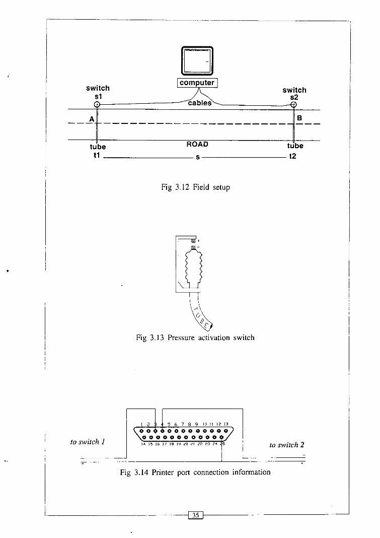
3.3.2 PRINCIPLE

Two active probes are fixed at the entry and exit sections at s distance apart.

Whenever a vehicle crosses at the entry section, the switch, which is connected at

the end of the probe will be activated. The computer will detect its current system

time t l at the time of activation of the switch, which is connected through the printer

port of the computer. When the vehicle crosses the exit section the same process will

repeat and the exit time t2 will be recorded.

Therefore the speed of the vehicle can be calculated as:

v - - distance travelled / time required

i.e. v - - s I ( t 2 - t l )

switch switch sl 9

s2

A B ----.----------------------- ---

1

tube ROAD tube

to switch 1

Fig 3.12 Field setup

Fig 3.13 Pressure activation switch

to switch 2

+

Fig 3.14 Printer port connection information

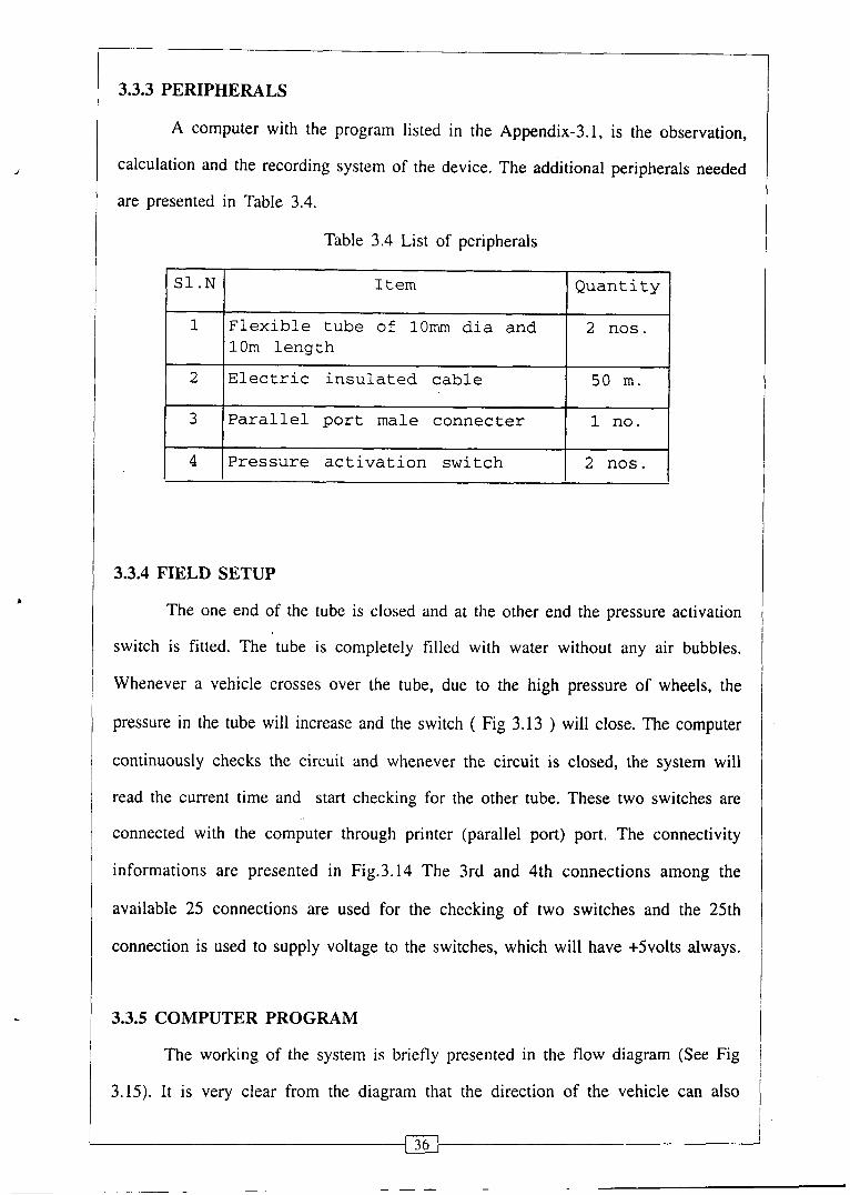
3.3.3 PERIPHERALS

A computer with the program listed in the Appendix-3.1, is the observation,

calculation and the recording system of the device. The additional peripherals needed

S1 .N Item Quantity

1 Flexible tube of 10mm dia and 2 nos. 10m length

2 Electric insulated cable 50 m.

3 Parallel port male connecter 1 no.

4 Pressure activation switch 2 nos.

3.3.4 FIELD SETUP

The one end of the tube is closed and at the other end the pressure activation

switch is fitted. The tube is completely filled with water without any air bubbles.

Whenever a vehicle crosses over the tube, due to the high pressure of wheels, the

pressure in the tube will increase and the switch ( Fig 3.13 ) will close. The computer

continuously checks the circuit and whenever the circuit is closed, the system will

read the current time and start checking for the other tube. These two switches are

connected with the computer through printer (parallel port) port. The connectivity

informations are presented in Fig.3.14 The 3rd and 4th connections among the

available 25 connections are used for the checking of two switches and the 25th

connection is used to supply voltage to the switches, which will have +5volts always.

/ 3.3.5 COMPUTER PROGRAM 1 l I The working of the system is briefly presented in the flow diagram (See Fig i

1 3.15). It is very clear from the diagram that the direction of the vehicle can also 1

1 automatically recorded by the program. The computer program is encoded in C I language and the program listing is presented in APPENDIX-3.1.

start 9 Read Total time

t2 = current tim

.I-,

is on 4

\I/

speed = S / (t2 - t l )

I

direction is 0 t 1 =current time

write speed & direction 5=

Fig 3.15 Flow chart for detecting entry and exit time of vehicles

s2 is on

V

direction is 1 t l =current time

I

The proposed methodology has no way to find the type of vehicle

automatically, which is coming to the test stretch. In order to incorporate the type of

vehicle also, the C program has been written to get a key from the user ( C for Car,

B for Bus, etc., ) so as to identify the type of the next vehicle coming to the test

section.

3.4 SUMMARY AND CONCLUSION

By the use of simple instrumentation set up proposed in this study, it is

possible to measure the distances of the moving vehicles from a chosen reference,

the speeds of the moving vehicles and the lateral placement of the vehicles. While,

the instrumentation set up is quite cheap and cost-effective, the potential of a laptop

computer is fully exploited for vehicle detection and study of lateral placements using

the number of pixels the vehicle images occupy on the computer monitor. This

procedure for vehicle detection and placement study avoids costly requirement of

pavement markings and uses the potential of modern computer thereby reducing the

manpower needed f i r conduct of survey.

APPENDIX - 3.1

VEHICLE DETECTION PROGRAM

This program listing (PORT.CPP) is to read the impact of vehicle wheels from the probes on the road so as to calculate the speed of the vehicle automatically on a PC connected to the probes through the printer port.

/

#include cstdio.h> #include cctype.h> #include cconio.h> #include cprocess.h> #include cstdlib.h> #include cstring.h #include cdos.h> #define Port Ox3bd

FILE *fpout;

main()

[ int i,count,inl=55,in2'=247,vtype,byte l ,byte2; int test,dir,vno[l2],total-no; char file~name[12],key,vehicle[l2],temp~str[25],direction[10]; struct time time-in,time-out; float timel,time2,time,distance,speed,temp~float; char temp-string[100]; clrscr();

print("\nEnter Distance between stations:"); scanf("%f ',&distance);

printf("\nEnter output file name:"); scanf("%s",&file-name);

clrscr(); if((fp~ut=fopen(file~name,"w"))==NULL)

(printf("\n\aError writing file"); exit(0);

1 outportb(Ox3bc, l);

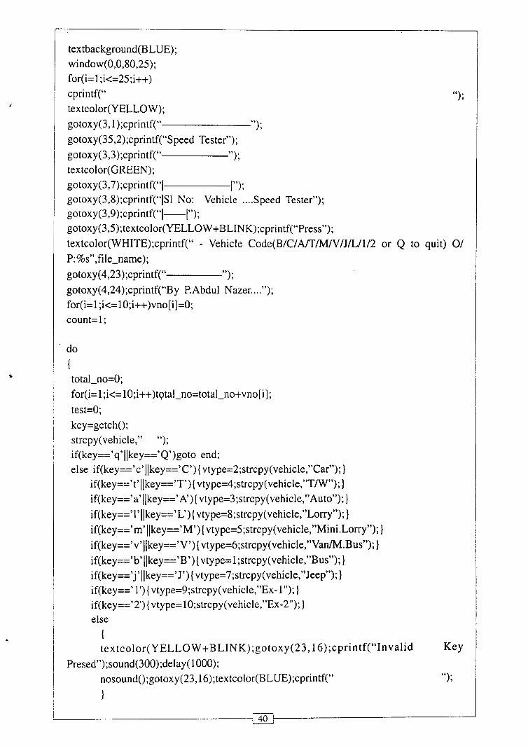
textbackground(BLUE); window(0,0,80,25); for(i= l ;i<=25;i++) cprintf(" "1; textcolor(Y ELL0 W); gotoxy(3,l);cprintf(" "1; gotoxy(35,2);cprintf("Speed Tester"); gotoxy(3,3);cprintf(" ");

textcolor(GREEN); gotoxy(3,7);cprintf("~ 1"); gotoxy(3,8);cprintf("~Sl No: Vehicle .... Speed Tester"); gotoxy(3,9);cprintf("I-I"); gotoxy(3,5);textcolor(YELLOW+BLINK);cprintf(b'Press"); textcolor(WHITE);cprintf(" - Vehicle Code(B/C/A/T/M/V/J/L/1/2 or Q to quit) 01 P: %sW,file-name); gotoxy(4,23);cprintf(" ">;

gotoxy(4,24);cprintf(By P.Abdu1 Nazer ...."); for(i=l ;i<= l O;i++)vno[i]=O;

test=O; key=getch(); strcpy(vehicle," ");

if(key=='q'llkey=='Q')goto end; else if(key=='c'llkey=='C') {vtype=2;strcpy(vehicle,"Car"); }

if(key=='t'Ilkey=='T') { vtype=4;strcpy(vehicle,"T/W"); } if(key=='a'Ilkey==' A') { vtype=3;strcpy(vehicle,"Auto"); }

if(key=='l'Ilkey=='L') {vtype=8;strcpy(vehicle,"Lorry"); ) if(key=='m' Ilkey=='M') {vtype=5;strcpy(vehicle,"Mini.L0rry"); } if(key=='v'/Ikey=='V') {vtype=6;strcpy(vehicle,"Van/M.Bus");} if(key=='b'Ilkey=='B') { vtype=l ;strcpy(vehicle,"Bus"); } if(key=='j'Ilkey=='J') {vtype=7;strcpy(vehicle,"Jeep");} if(key==' 1') {vtype=9;strcpy(vehicle,"Ex- 1 ");l if(key=='2') { vtype= lO;strcpy(vehicle,"Ex-2"); } else

{ textcolor(YELLOW+BLINK);gotoxy(23,16);cprintf(bbInvalid Key

Presed");sound(300);delay( 1000); nosound();gotoxy(23,16);textcolor(BLUE);~printf(~~ "1;

1

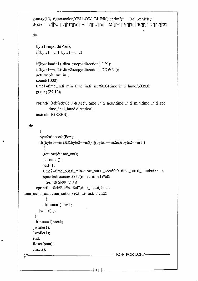
do

{ byte l =inportb(Port); if(byte l ==in l ((byte l==in2)

I if(bytel==inl){dir=l;srcpy(direction,"UP"); if(byte 1 ==in2) (dir=2;srcpy(direction,"DOWN"); gettime(&time-in); sound(1000); time 1 =time-in.ti-min+time-in. ti~sec/60.0+time~in.ti~hund/6000.0; gotoxy(24,16);

time~out.ti~min,time~out.~ti~sec,time~in,ti~hund);

1 if(test== 1)break;

} while(1);

1 if(test== 1)break;

} while(1); } while(1); end: flose(fpout); clrscr();

1 11 EOF PORT.CPP