Distributed Facility Location Algorithms for FlexibleConfiguration of Wireless Sensor Networks

Christian Frank and Kay Romer

Department of Computer ScienceETH Zurich, Switzerland

{chfrank,roemer}@inf.ethz.ch

Abstract. Many self-configuration problems that occur in sensor networks, suchas clustering or operator placement for in-network data aggregation, can be mod-eled as facility location problems. Unfortunately, existing distributed facility lo-cation algorithms are hardly applicable to multi-hop sensor networks. Based onan existing centralized algorithm, we therefore devise equivalent distributed ver-sions which, to our knowledge, represent the first distributed approximationsof the facility location problem that can be practicably implemented in multi-hop sensor networks with local communication. Through simulation studies, wedemonstrate that, for typical instances derived from sensor-network configurationproblems, the algorithms terminate in only few communication rounds, the run-time does not increase with the network size, and, finally, that our implementationrequires only local communication confined to small network neighborhoods. Inaddition, we propose simple extensions to our algorithms to support dynamicnetworks with varying link qualities and node additions and deletions. Using linkquality traces collected from a real sensor network deployment, we demonstratethe effectiveness of our algorithms in realistic multi-hop sensor networks.

1 Introduction

An important problem in wireless sensor networks [1] is self-configuration [2], wherenetwork nodes take on different functions to achieve a given application goal. One ex-ample is clustering [3], where some nodes are elected as cluster leaders, serving ascommunication hubs for nearby nodes. A similar problem is aggregator placement [4],where some nodes are elected as aggregators that collect and aggregate sensor datafrom nearby sensor nodes. Recently, tiered sensor networks [5] have been proposed,consisting of resource-poor sensor nodes in the first tier and powerful hub nodes in thesecond tier. In these networks, every sensor node is assigned to and controlled by ahub node. Note that in all of the above examples, self-configuration consists in electingsome nodes as servers while the remaining client nodes are assigned to a server.

While many proposals exist for finding such network configurations, they often donot pay attention to optimizing the overall cost of these configurations, which consistsof two components: on the one hand, the costs of operating the servers (e.g., represent-ing the servers’ increased communication load as these forward traffic for many clients),and, on the other hand, the costs of communication between clients and their server. Inwireless networks, the latter cost can be dependent on the physical distance between a

client and its server (as a longer wireless link requires higher transmit power and thusincreased energy consumption), on the number of hops in a multi-hop network graph,or on interference and network congestion. In all cases, lowering communication costsby means of additional hub nodes may prove beneficial.

Our goal is to provide a generic and practical mechanism for finding cost-optimizedsolutions to the above self-configuration problems. Our approach is based on the obser-vation that the above optimization problem can be modeled as an (uncapacitated) facil-ity location problem. There, we are given a set F of facilities, a set C of clients (alsoknown as cities or customers), a cost fi for opening a facility i ∈ F and connectioncosts cij for connecting client j to facility i. The objective is to open a subset of facil-ities in F and connect each client to an open facility such that the sum of connectionand opening costs is minimized.

Although the facility location problem has been studied extensively in the past, nopractical solutions exist that would be suitable for multi-hop sensor networks. Whiledistributed algorithms for facility location exist, they are either not generally applicable[6], require a certain (albeit small) amount of global knowledge [7], require impracticalcommunication models [7,8], or (based on the provided approximation factor [8]) mightnot improve over existing configuration heuristics for sensor networks.

We therefore contribute a local facility location algorithm that lends itself well forimplementation in multi-hop sensor networks and provides an approximation factorof 1.61 for metric instances. By means of an experimental study, we show that thealgorithm terminates after few communication rounds for typical problem instancesderived from sensor network configuration problems.

While the above view adopts a static graph model of sensor networks, practicalsensor networks are rather dynamic: nodes may fail and the quality of wireless linksfluctuates over time. To make our algorithm applicable to such realistic settings, wepropose a set of rules to repair a sensor network configuration in case of node failures,additions, and link quality changes. Also, we study the optimality of our algorithm usinglink quality traces collected from a real sensor network deployment.

2 Preliminaries

We model the multi-hop network subject to configuration as a graph G = (V,E). Inour application of the facility location problem, a network node takes on the role ofa client and that of a potential facility at the same time, that is, F = C = V . Insome cases, only a subset nodes have the necessary capabilities (e.g., remaining energy,available sensors, communication bandwidth, or processing power) to execute a service.In such cases, the nodes eligible as facilities can be selected beforehand based on theircapabilities [9], which results in F ⊆ C = V . When clients are connected to facilities,we will use σ(j) to refer to the facility that connects a client j.

Based on the problem at hand, one may choose a particular setting of opening costsfi and connection costs cij . In most settings, for a network link (i, j) ∈ E, the respec-tive communication cost cij will be set to some link metric that can be determined lo-cally at the nodes, e.g., based on dissipated energy or latency. Some approximation algo-rithms require that the costs cij constitute a metric instance. A metric instance requiresthat, for any three nodes i, j, k, the direct path is shorter than a detour (cij ≤ cik + ckj).

However, if connection costs cij should represent the transmit power used for sending,these are often proportional to the square of the geographic distance between i and j,which results in non-metric instances, for example:

i j

k4

8

1

If the input to a facility location algorithm is non-metric, the problem is particularlyhard to solve (see Section 3 below). However, one may obtain a metric instance byignoring non-metric links and setting cij to the cost of a shortest path between twonodes i and j. In multi-hop networks, the required shortest-paths computation can beachieved using a local flood around the current node.

When addressing settings in which facilities and clients can be an arbitrary num-ber of network hops apart, we will always compute cij via shortest-paths. We refer tothis metric problem setting as multi-hop. Alternatively, we will consider a second (con-strained) version of the problem, in which we require that every client is connectedto a facility which is its direct network neighbor. We denote this constrained problemdefinition as one-hop. One-hop instances are inherently non-metric, as missing links(i, j) /∈ E, modeled by cij = ∞, violate the metric property.

3 Related Work

An ample amount of literature exists on (centralized) approximation algorithms for theNP-hard facility location problem [10]. Such centralized algorithms are not applicableas these would require a prohibitive communication overhead associated with collectingthe whole network topology at a single point (e.g., at the network basestation).

For non-metric instances of the facility location problem, even approximations arehard to come by: As the set cover problem can be reduced to (non-metric) facility lo-cation, the best achievable approximation ratio (even with a centralized algorithm) islogarithmic1 in the number of nodes [11]. A classic and simple algorithm [12] alreadycomes close to this lower bound. Distributed approximations are rare: [7] solve non-metric facility location even in a constant number of communication rounds. However,the algorithm requires that a coefficient ρ, which is computed from a global view ofthe problem instance, is distributed to all nodes before algorithm execution – whichprevents it from being used “as-is” in practice. Moreover, the algorithm requires globalcommunication among all relevant clients and facilities and therefore can only effi-ciently be used in the one-hop setting where such communication can be implementedefficiently by wireless broadcast. Finally, the best approximation factor it can obtain,which is independent of the problem instance, is on the order of O(log(m+n) log(mn))where m and n denote the number of facilities and clients, respectively.

For metric instances of the facility location problem, much better approximationfactors ∈ O(1) can be achieved. While it has been shown [13] that a polynomial-timealgorithm cannot obtain an approximation ratio better than 1.463, a centralized algo-rithm [14] already provides a solution that is at most a factor of 1.52 away from theoptimum. For the metric case, to our knowledge only one distributed algorithm has

1 This holds unless every problem in NP can be solved in O(nO(log log n)) time.

been mentioned [8] which solves only a constrained version of the problem in whichfacilities and clients may be at most 3 hops away. It provides a 3+ ε approximation fac-tor derived from a parallelized execution of a respective centralized algorithm [15] andis formulated in terms of a synchronous message passing model. The same paper [8]includes additional versions, which restrict the facility location problem in one wayor another. Only recently, a highly-constrained version of the facility location problemhas been addressed in a distributed manner [6]. Finally, a distributed algorithm basedon hill-climbing [16] addresses a version of the problem in which exactly k facilitiesare opened. However, the worst-case time complexity and the obtained approximationfactor are not discussed explicitly.

In this paper, we develop a distributed version of a centralized algorithm [17] whichprovides an 1.61 approximation factor with metric instances. Compared to related work,our work improves on the approximation factor achievable in a distributed manner.Moreover, we provide the adaptations required to execute this algorithm in multi-hopnetworks for which, to our knowledge, no efficient algorithm with guaranteed worst-case approximation factor exists. Finally, compared to [7,8], our algorithms do not re-quire a synchronous message passing model. Instead, they perform synchronizationamong network neighbors implicitly as nodes wait for incoming messages.

In the remainder of the paper, we briefly summarize the centralized approximationalgorithms [17] our work is based on in Section 4. We then describe their distributedre-formulation in two steps. The first variant, in Section 5, still requires global commu-nication, namely that all clients communicate with all relevant facilities in each step,and is therefore only applicable to the one-hop setting, where this can be efficientlyimplemented as a wireless broadcast. In the second step, we use this algorithm as asubroutine in the algorithms of Section 6, which distribute messages only to a localneighborhood around the sending node and may therefore be used in multi-hop net-works. Finally, we provide experimental results in Section 7 and an outlook to futurework in Section 8.

4 Centralized Algorithms

Jain et al. [17] devised two centralized approximation algorithms for the facility locationproblem. Both use the notion of a star (i, B) consisting of a facility i and an arbitrarychoice of clients B ⊆ C (in clustering terminology, a star corresponds to a clusterleader and a set of associated slave nodes). The first is shown in Algorithm 1. In its corestep (line1.3), the algorithm selects the star (i, B) with best (lowest) cost efficiency. Thecost efficiency of a star is defined as

c(i, B) =(fi +

∑cij

)/|B| (1)

and represents the average cost per client which this star adds to the total cost.Therefore, in each step, the algorithm selects the most cost-efficient star (i, B),

opens the respective facility i, connects all clients j ∈ B to i (sets σ(j) = i), and fromthis point on disregards all (now connected) clients in B. The algorithm terminates onceall clients are connected.

Algorithm 1: Centralized 1.861-approximation algorithm [17]set U = C1.1while U 6= ∅ do1.2

find most cost-efficient star (i, B) with B ⊆ U1.3open facility i (if not already open)1.4set σ(j) = i for all j ∈ B1.5set U = U \B1.6set fi = 01.7

Note that in spite of there being exponentially many sets B ⊆ U , the most efficientstar can be found in polynomial time: For each facility i, clients j can be sorted byascending connection cost to i. Any most cost-efficient star spanning some k = |B|clients will consist of the first k clients with lowest connection costs – all other subsetsof k clients can be disregarded as these cannot be more efficient. Hence, at most |C|different sets must be considered.

When a facility i is opened, its opening cost fi is set to zero. This allows facilityi to be chosen again to connect additional clients in later iterations, based on a cost-efficiency that disregards i’s opening costs fi – as the facility i has already been openedbefore in order to serve other clients. For metric instances, Algorithm 1 provides a1.861 approximation factor. Note that line 1.7 constitutes the only difference to a classicalgorithm [12], whose approximation factor for metric instances is much worse. Aneven better approximation factor of 1.61 can be obtained when changing the abovealgorithm to additionally take into account the benefit of opening a facility i for clientsthat are already connected to some other facility. This involves two changes.

First, this requires that a revised cost-efficiency definition is used in line 1.3. We letB(i) denote the set of clients j which are already connected to some facility σ(j) andwould benefit if i would be opened as their connection cost to i would be lower thantheir current connection cost cσ(j)j , i.e.,

B(i) ={j ∈ C with σ(j) 6= none and cij < cσ(j)j

}. (2)

The cost efficiency of a star (i, B) can now be restated as

c(i, B) =

fi +∑j∈B

cij −∑

j∈B(i)

(cσ(j)j − cij)

/|B|. (3)

A second analogous change is made to line 1.5. In addition to the clients which are partof the most-efficient star (i, B), all already-connected clients B(i) which benefit fromswitching are connected to i. For this, line 1.5 becomes

set σ(j) = i for all j ∈ B ∪B(i).

The authors prove [17] that this change improves the approximation factor to 1.61 formetric instances. In the following, we will present a distributed version of this 1.61-algorithm. In the discussed distributed adaptations, we will always use the revised cost-efficiency definition of Eq. (3).

5 One-hop Approximation

Consider the distributed algorithms given in Algorithm 2 (for facilities) and 3 (forclients). We will show below that they perform the exact same steps as the centralizedAlgorithm 1. While these algorithms require that each client communicates with eachfacility and vice versa, the algorithms can be also applied “locally” such that each nodecommunicates only with its network neighbors. This way, they can be used to com-pute a solution to the one-hop version of the facility location problem, for example, tocompute an energy-efficient clustering that takes costs of individual links into account.Unfortunately, this constrained problem version results in a non-metric instance (seeSection 2) and thus the approximation guarantee of 1.61 cannot be preserved. However,in the next section, we will use these algorithms as a subroutine to obtain an algorithmthat maintains the approximation factor of 1.61 for multi-hop sensor networks. More-over, we will show that it computes good solutions, nevertheless, in our experimentalresults of Section 7.

We assume that after an initial neighbor discovery phase, each client j knows theset of neighboring facilities, which it stores in the local variable Fj , and the connectioncosts cij to facilities i ∈ Fj . Vice versa, each facility i knows the set of neighboringclients Ci and cij of all i ∈ Ci. In the following we will simply write C and F , as therespective indices i and j can be deduced from the context.

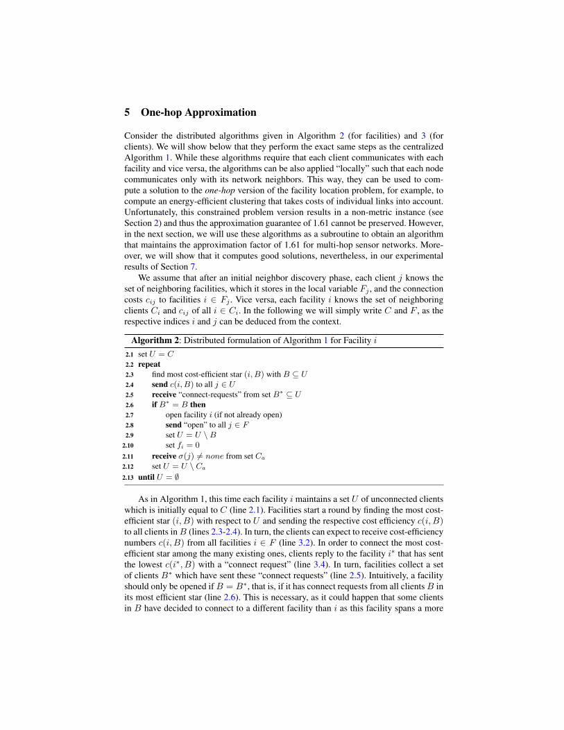
Algorithm 2: Distributed formulation of Algorithm 1 for Facility i

set U = C2.1repeat2.2

find most cost-efficient star (i, B) with B ⊆ U2.3send c(i, B) to all j ∈ U2.4receive “connect-requests” from set B∗ ⊆ U2.5if B∗ = B then2.6

open facility i (if not already open)2.7send “open” to all j ∈ F2.8set U = U \B2.9set fi = 02.10

receive σ(j) 6= none from set Ca2.11set U = U \ Ca2.12

until U = ∅2.13

As in Algorithm 1, this time each facility i maintains a set U of unconnected clientswhich is initially equal to C (line 2.1). Facilities start a round by finding the most cost-efficient star (i, B) with respect to U and sending the respective cost efficiency c(i, B)to all clients in B (lines 2.3-2.4). In turn, the clients can expect to receive cost-efficiencynumbers c(i, B) from all facilities i ∈ F (line 3.2). In order to connect the most cost-efficient star among the many existing ones, clients reply to the facility i∗ that has sentthe lowest c(i∗, B) with a “connect request” (line 3.4). In turn, facilities collect a setof clients B∗ which have sent these “connect requests” (line 2.5). Intuitively, a facilityshould only be opened if B = B∗, that is, if it has connect requests from all clients B inits most efficient star (line 2.6). This is necessary, as it could happen that some clientsin B have decided to connect to a different facility than i as this facility spans a more

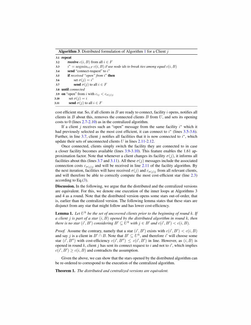
Algorithm 3: Distributed formulation of Algorithm 1 for a Client j

repeat3.1receive c(i, B) from all i ∈ F3.2i∗ = argmini∈F c(i, B) // use node ids to break ties among equal c(i, B)3.3send “connect-request” to i∗3.4if received “open” from i∗ then3.5

set σ(j) = i∗3.6send σ(j) to all i ∈ F3.7

until connected3.8on “open” from i with cij < cσ(j)j3.9

set σ(j) = i3.10send σ(j) to all i ∈ F3.11

cost efficient star. So, if all clients in B are ready to connect, facility i opens, notifies allclients in B about this, removes the connected clients B from U , and sets its openingcosts to 0 (lines 2.7-2.10) as in the centralized algorithm.

If a client j receives such an “open” message from the same facility i∗ which ithad previously selected as the most cost efficient, it can connect to i∗ (lines 3.5-3.6).Further, in line 3.7, client j notifies all facilities that it is now connected to i∗, whichupdate their sets of unconnected clients U in lines 2.11-2.12.

Once connected, clients simply switch the facility they are connected to in casea closer facility becomes available (lines 3.9-3.10). This feature enables the 1.61 ap-proximation factor. Note that whenever a client changes its facility σ(j), it informs allfacilities about this (lines 3.7 and 3.11). All these σ(j) messages include the associatedconnection costs cσ(j)j and will be received in line 2.11 of the facility algorithm. Bythe next iteration, facilities will have received σ(j) and cσ(j)j from all relevant clients,and will therefore be able to correctly compute the most cost-efficient star (line 2.3)according to Eq.(3).Discussion. In the following, we argue that the distributed and the centralized versionsare equivalent. For this, we denote one execution of the inner loops at Algorithms 3and 4 as a round. Note that the distributed version opens some stars out-of-order, thatis, earlier than the centralized version. The following lemma states that these stars aredisjunct from any star that might follow and has lower cost-efficiency.

Lemma 1. Let Uk be the set of uncovered clients prior to the beginning of round k. Ifa client j is part of a star (i, B) opened by the distributed algorithm in round k, thenthere is no star (i′, B′) considering B′ ⊆ Uk with j ∈ B′ and c(i′, B′) < c(i, B).

Proof. Assume the contrary, namely that a star (i′, B′) exists with c(i′, B′) < c(i, B)and say j is a client in B′ ∩ B. Note that B′ ⊆ Uk, and therefore i′ will choose somestar (i′, B′′) with cost-efficiency c(i′, B′′) ≤ c(i′, B′) in line. However, as (i, B) isopened in round k, client j has sent its connect request to i and not to i′, which impliesc(i′, B′) ≥ c(i, B) and contradicts the assumption.

Given the above, we can show that the stars opened by the distributed algorithm canbe re-ordered to correspond to the execution of the centralized algorithm.

Theorem 1. The distributed and centralized versions are equivalent.

Proof. We sequentialize the distributed algorithm as follows: In the sequentialized ver-sion we open only one star (the globally most cost-efficient star) per round. Further,we postpone opening a star (i, B) which has been opened in parallel by the distributedalgorithm to a later round prior to which all stars (i′, B′) with c(i′, B′) < c(i, B) havebeen processed. Let (i′, B′) denote one such star. Because of Lemma 1, B′ ∩ B = ∅,and therefore opening (i′, B′) ahead of time does not remove any client in B from Uand therefore does not interfere with opening (i, B). Similarly, postponing any (i, B)will not allow that a more cost-efficient star including elements of B is formed earlier– again by Lemma 1. Postponing (i, B) can further influence (raise) the cost-efficiencyof the stars (i′, B′) as it changes the set B(i) for these facilities and thus may changethe order in which these are processed. However, as by Lemma 1 all these stars are mu-tually disjunct, the order in which they are opened does not affect total costs. Finally,all stars opened in parallel are disjunct and re-ordering them does not change algorithmexecution.

Therefore, the sequentialized version opens the same stars as the distributed algo-rithm. Moreover, as the sequentialized version opens the most cost-efficient star in everyround, it implements the execution of the centralized algorithm.

Nevertheless, the worst-case number of rounds required by Algorithms 2 and 3 re-mains linear in the number of nodes, because there can be a unique point of activityaround the globally most cost-efficient facility i∗ in each round: Consider for instance achain of m facilities located on a line, where each pair of facilities is interconnected byat least one client, and assume that facilities in the chain have monotonously decreas-ing cost efficiencies. Each client situated between two facilities will send a “connect-request” to only one of them (the more cost efficient), thus the second cannot open.In this example, only the facility at the end of the chain can be opened in one round.Similarly, once at least one facility is open, it could happen that in each round only oneclient connects to this facility. The worst-case runtime is therefore O(n), in which n isthe number of network nodes.

The linear number of rounds required in the worst-case would constitute a veryhigh overhead in large-scale sensor networks. However, a worst-case configuration ona larger scale is highly improbable (as we will show in Section 7), and the approxima-tion factor inherited from the centralized version is intriguing, particularly because thealgorithm performs even much better than 1.61 on average instances. We will evaluatethe average number of rounds required for typical instances in sensor networks and theoptimality gap when the algorithm is executed with such instances in Section 7.

As we mentioned, however, the above algorithm only retains its approximation fac-tor with metric instances, and as any metric instance is essentially a complete graph, itrequires global communication between all clients and facilities. This is only efficientin few settings, for example when all nodes hear each other over the wireless broadcastmedium. In the next section we use the algorithms of this section as subroutines in anadapted “local” version that functions properly in multi-hop networks.

6 Multi-hop Approximation

The described algorithm can be changed to work in multi-hop settings using only aslight adaptation. As it turns out, if connection costs represent shortest paths between

Algorithm 4: Multi-Hop Adaptation of Algorithm 3 for a Client j

set s = 1, set σ(j) = none4.1repeat4.2

set s = s× a4.3send “start(s)” to all i ∈ Fs4.4if no “begin(s)” received then continue4.5repeat4.6

receive c(i, B) from all facilities Fs4.7set Fa = {i ∈ Fs with c(i, B) ≤ s}4.8if Fa 6= ∅ then4.9

i∗ = argmini∈Fa c(i, B) // use node ids to break ties4.10send “connect-request” to i∗4.11if received “open(s)” from i∗ then4.12

set σ(j) = i∗4.13send σ(j) to all i ∈ Fs4.14

until connected or Fa = ∅4.15

until connected4.16on “open(s∗)” from i with cij < cσ(j)j4.17

set σ(j) = i4.18send σ(j) to all i ∈ Fs∗4.19

network nodes, the communication performed by the algorithms can be restricted tosmall network neighborhoods. Specifically, if one is interested in determining whethera facility i has a cost-efficiency of less than a certain threshold s, it is sufficient toconsider only clients j that are reachable by i over a path with costs of at most s, i.e.,clients j with cij ≤ s. To see this, consider the definition of a facility’s cost-efficiencyand assume that some star’s cost efficiency c(i, B) ≤ s. One can always obtain an evensmaller cost-efficiency once one removes the clients j ∈ B′ which have cij > s, thatis, c(i, B \B′) < c(i, B). Similarly, given a facility i, the clients with cσ(j)j > cij willnot occur in the set B(i) of Eq. (3). Therefore, it is sufficient that clients j which arenewly connected to σ(j) distribute σ(j) only to facilities i with cost cij < cσ(j)j .

In an outer loop added around Algorithms 2 and 3, we therefore exponentially in-crease the communication scope s, that is, the maximum distance over which messagesare forwarded. Specifically, given a certain scope s, a message is only flooded withina localized neighborhood Ns(i) around the sending node i, where Ns(i) := {j ∈V with cij ≤ s}. Note that if the direct link (i, j) is not present in the network graph,cij representing the shortest path from j to i can be determined on the fly while floodinga message within Ns(j). Nodes simply stop forwarding a message if it has covered adistance of larger than s or if it has already been received over a shorter path.

The updated versions are given in Algorithm 4 (clients) and Algorithm 5 (facilities).In the following, we will respectively use Cs and Fs to refer to client and facility nodeswithin scope s of the current node.

In the outer loop, the considered scope s is raised exponentially (lines 4.3 and 5.3).To initialize an outer round, clients, which have not yet been connected, send a “start”message containing their current scope s to all facilities in scope (line 4.4). In turn,facilities wait for at least one such “start” message for a certain time (line 4.5) uponwhich they reply “begin(s)”. The waiting period must be long enough to allow relevant

Algorithm 5: Multi-Hop Adaptation of Algorithm 2 for Facility i

set s = 15.1repeat5.2

set s = s× a5.3if “start(s)” received then send “begin(s)” to all j ∈ Cs else continue5.4query σ(j) from all j ∈ Cs5.5set Us = {j ∈ Cs with σ(j) = none}5.6repeat5.7

find most cost-efficient star (i, B) with B ⊆ Us5.8send c(i, B) to all j ∈ Us5.9if c(i, B) ≤ s then5.10

receive “connect-requests” from set B∗ ⊆ Us.5.11if B∗ = B then5.12

open facility i (if not already open)5.13send “open(s)” to all j ∈ C5.14set Us = Us \B, set fi = 05.15

receive σ(j) 6= none from some clients B′ ⊆ Us5.16set Us = Us \B′5.17

until Us = ∅ or c(i, B) > s5.18

until s > smax5.19

clients to send the respective start messages and finish earlier rounds. If no “start” mes-sages were received, facilities simply advance to the next outer round (line 5.4) to waitfor “start” messages from a larger scope. Clients, analogously, wait and then skip thecurrent round if no neighboring facility has sent “begin”.

A start message sent by a client j thus triggers execution of one outer round at allthe facilities in scope Fs. Facilities then query all clients in scope for their status σ(j)in line 5.5 and compute the set of yet unconnected clients Us. This query-reply cycle al-lows the facility to wait for all relevant clients to catch up to the current scope s. Clientsreply to this query once they have reached scope s – note that we have omitted therespective code in the client algorithm. Similarly clients can wait for facilities laggingbehind in line 4.7 where they expect to receive a message from all facilities in scope.

After this initialization, facilities execute Algorithm 2 in an inner loop (lines 5.7-5.18) and clients react accordingly (lines 4.6-4.15) implementing Algorithm 3. Com-pared to Algorithms 2 and 3 the termination conditions of the inner loops must bechanged to allow clients and facilities to proceed to a larger scope in a properly synchro-nized manner. As with the 1-hop version, clients terminate their inner loop once they areconnected (line 4.15) and facilities once no active clients remain in scope (line 5.18).In addition, within an inner-loop with scope s, the algorithm should only consider stars(i, B) with cost-efficiency c(i, B) < s. Therefore, facilities only proceed with the cur-rent inner loop as long as they are efficient enough for this scope (lines 5.10 and 5.18)while in turn clients only proceed with their inner loop as long as there is a facility inscope that is efficient enough to connect them (lines 4.8,4.9 and 4.15).

Finally, once a client has been connected (4.17-4.19), it acts analogously to Al-gorithm 3: It simply changes its facility if this is beneficial and notifies all relevantfacilities about it. Here the client can synchronize to the scope s∗ of the sending facilityas it is included in the received “open” message to ensure that all relevant facilities are

informed. Note that the messages sent in line 4.19 are also received by facilities stillperforming their inner loop in line 5.16.Discussion. The algorithms presented in this section enhance Algorithms 3 and 4 bymaking them “local”, meaning that they do not need to communicate with all relevantfacilities but only to the ones within a confined neighborhood. This allows to performshortest-paths computations in these confined neighborhoods which, in turn, give riseto metric instances and preserve the approximation factor of Algorithm 1.

An additional outer loop provides for both, an adequate expansion of the involvedcommunication scope and for sufficient synchronization of the nodes in scope with-out depending on a synchronized communication model. Because clients and facilitiesmay repeatedly have to wait in lines 4.5 and 5.4, respectively, the worst-case runtimebecomes O(n loga smax) where smax denotes the cost efficiency of the least efficientstar which occurs in the network and n denotes the total number of participating nodes.However, the maximum number of rounds involving actual communication is smaller.If no unconnected clients or eligible facilities are present, the involved nodes do notcommunicate in their inner loop at all. Instead, they simply skip the inner loop. In turn,in rounds involving communication, a client or facility can be a single point of activityonly once during algorithm execution. Therefore, the number of required communica-tion rounds is still in O(n).Dynamic Re-configuration. In real-world deployments of sensor networks, link qual-ities change over time and nodes may fail. To accommodate for major changes in thenetwork topology, the algorithms are re-executed at regular intervals. As such re-startsinvolve relatively high overhead, these are performed only infrequently (e.g., once aday). In between such re-starts, a client j combines periodic re-evaluations of link costscij (within a local scope of size cσ(j)j) with a liveness check on the facility σ(j). In bothcases, if σ(j) has failed or a closer open facility has been found, client j re-connectsto the closest open facility. In Section 7, we will show that such adaptations suffice tomaintain a close-to-optimal configuration over longer periods of time.

7 Experimental Results

In the following, we show results from two distinct sets of experiments. The first, de-tailed in Section 7.1, is based on simulations which test the scalability of the proposedalgorithms. The second, detailed in Section 7.2 tests the applicability of the proposedalgorithms to operational networks with dynamic links.

7.1 Scalability

In the experiments based on simulations, we uniformly deployed a variable number ofnodes (x-axis) onto a 300m by 300m area. The network graph has an edge (i, j) ∈ E ifthe nodes i and j are less than 30m apart (this number stems from a model that is basedon the characteristics of the CC1000 transceiver used on BTnodes [18] and BerkeleyMotes). Assuming that nodes can control their transmit power, for (i, j) ∈ E, we setconnection costs cij ∼ g(i, j)2 where g(i, j) denotes the distance in meters between iand j and normalize them such that cij ∈ [0, 1].

Scenarios. To test our algorithms with a range of applications, we examined three dif-ferent parameterizations of the facility location problem, of which qualitative results areshown in Figure 1. In the first, we set opening costs fi = 1 and additionally require thatclients and facilities must be neighbors. We show a solution obtained by the one-hopAlgorithms 2 and 3 on such an instance in Figure 1(a).

Further, we tested the multi-hop Algorithms 4 and 5 in two different settings. In thefirst, we set fi = 5 to denote that a high effort is required to operate a cluster leader,of which an example result is shown in Figure 1(b). In the second scenario, shownin Figure 1(c), we assumed that cluster leaders must send much data to the networkbasestation and therefore their operation costs increase with their network distance tothe sink (yielding smaller stars close to the sink and larger ones further away).

(a) fi = 1 (b) fi = 5 (c) fi = 2×D(sink, i)

Fig. 1. Effects of varying opening costs (D(sink, i) denotes the shortest-path distanceto the sink, which is located in the upper left corner of the simulated area)

One-Hop Clusters. In the one-hop setting (Figure 1(a)), we evaluated the costs ofconfigurations produced by different algorithms while varying the number of nodes inthe simulation area (that is, the node density). The results are given in Figure 2(a) whichshows the costs obtained with the following five methods.

One-hop denotes the simple one-hop algorithms of Section 5. Respectively, one-hopIP refers to the optimal configuration of the constrained case which requires clients toconnect to facilities which are direct network neighbors. Further, multi-hop denotes themulti-hop algorithm described in Section 6, which has a 1.61 approximation guarantee.Here, clients may connect to facilities which are an arbitrary number of hops away. Re-spectively, multi-hop-IP computes the optimal solution to the facility location problem,in which facilities and clients may be multiple hops apart and the instance is made met-ric by a centralized shortest-paths computation. Finally, MDS-IP denotes the optimalsolution to the minimum dominating set problem, in which dominator nodes representopen facilities and slave nodes are clients that connect to the closest dominator node.The costs are computed using the original (non-metric) instance.

The costs of a minimum dominating set (MDS-IP) which suffer from expensivelong links mark one end of the optimization spectrum. Here we argued that facility lo-cation can provide a more energy efficient configuration. On the other hand, the optimalfacility-location based configuration (multihop-IP) marks the other end as it representsa lower bound for the employed approximation algorithms.

80

100

120

140

160

180

200

220

240

260

200 250 300 350 400 450 500

Cos

ts

Number of nodes

one-hopone-hop IP

multi-hopmulti-hop IP

MDS IP

(a) One-hop

180

200

220

240

260

280

300

320

340

200 250 300 350 400 450 500

Cos

ts

Number of nodes

distdist IPsimple

simple IP

(b) Multi-hop

Fig. 2. Performance of one-hop and multi-hop algorithms

The one-hop algorithm performs well and is even close to the respective optimalconfiguration one-hop IP, although it operates on a non-metric instance and thus with-out a guaranteed approximation factor.

Note that in this particular setting, the constrained versions, which require facilitiesand clients to be direct neighbors (one-hop and the optimal one-hop IP), are not far awayfrom the multi-hop results and the optimum of the unconstrained case (multi-hop IP).This is due to the low opening costs we used, which are set to fi = 1 for all facilities.With larger opening costs, multi-hop solutions would benefit more from larger stars.

Multi-Hop Clusters. In the experiments shown in Figure 2(b), we additionally evaluatethe quality of the solutions obtained by the multi-hop algorithm with the two differentopening cost settings shown in Figures 1(b) and 1(c). In the first (denoted as simple) weset opening costs to a constant fi = 5 which corresponds to configurations as shown inFigure 1(b). In the second, denoted as dist, we apply the heuristic shown in Figure 1(c),where the opening costs correspond to twice the costs of the shortest path to the sink. Inboth cases, the results of the distributed implementation are very close to the achievableoptimum computed by CPLEX on the same instance.

Runtime and Overhead. In the experiments shown in Figure 2(b), the scope s startedout with 0.2 and a was set to 2, thus doubling the scope in each outer round. Note,however, that these two parameters do not influence the quality of the obtained solution.Rather, they determine the trade-off achieved between the runtime of the algorithms andthe scope within which messages are sent. On the one hand, the smaller a is set, the moreone may be sure that scopes are not increased too far (in vain). On the other hand, therequired number of outer rounds until termination increases with lower a-values.

Figure 3 demonstrates this trade-off as observed in the simulation run correspondingto Figure 2(b). In Figure 3(a) we show the average scope with which messages were sentduring algorithm execution, given different settings of a (the scope s always starts at0.2). The lower we set a, the better the results as the scope is increased by smalleramounts. Note that in general, the effort involved in the execution of our algorithmis proportional to the “locality” implied by the problem instance: On the one hand, ifopening costs are high (here fi = 5), a facility will generally connect clients in a larger

neighborhood (as seen in Figure 1(b)). On the other hand, the experienced scopes areeven much lower with small opening costs (e.g., for fi = 1, not shown).

0.5

1

1.5

2

2.5

3

200 250 300 350 400 450 500

Ave

rage

sco

pe s

ize

Number of nodes

a=2.0a=1.5a=1.2a=1.1

(a) Scope

10

15

20

25

30

35

40

45

50

55

200 250 300 350 400 450 500

Run

time

(in r

ound

s)

Number of nodes

a=2.0a=1.5a=1.2a=1.1

(b) Rounds

Fig. 3. Average scope size vs. total runtime (in rounds). In Figure 3(b) the error barsdenote the maximum and the minimum that occurred.

In contrast, in Figure 3(b), we show the runtime in rounds (one round correspondsto one execution of the inner loop) of the multi-hop algorithm on the same instances.Note that, while previously the error bars indicated confidence intervals of 95%, we usethem in Figure 3(b) to mark the maximum and minimum values that occurred in 10random instances (as we are particularly interested in the maximum value). The resultsshow that – while in theory the worst case runtime can be large – in typical instancesbased on multi-hop networks the runtime is sufficiently small and does not even growwith the number of nodes. Moreover, based on the trade-off between runtime and scopesize, the runtime improves with higher a values. Finally, the scope size decreases withincreasing network density. This is due to the fact that, given certain opening costs,the algorithms will connect stars of around the same size (namely, facilities are openedonce enough clients are connected to pay for opening them). Therefore, smaller starsare opened in denser networks and the cumulated communication overhead stays thesame.

7.2 Network Dynamics

One open question is whether such, albeit close-to-optimal solutions, can provide abenefit for real-world deployments in which the network topology changes over time.To obtain realistic link qualities, we extended a testbed of 13 TMote Sky modulesthat gather temperature, humidity, and light measurements from our office premisesto record network topology information as well. Next to its sensor measurements, every5 seconds, a node reports the set of nodes from which an application-layer message hasbeen received since the last update.

Such topology information received from each node i allows to compute a (packet-level) link quality estimate eij(t) for each network link directed from j to i [19]. Theestimate eij(t) is based on the packet success rate rij = packets received in T

packets expected in T whichis smoothened using an exponentially weighted moving average such that eij(t) =

αrij(t) + (1 − α)eij(t − 1). In our experiments, we set α=0.6 according to [19] andT to 300 s. We transform the quality estimates eij ∈ [0, 1] into link cost estimates bysetting cij = 1 + 10(1 − eij) if eij > 0.5 and cij = ∞, otherwise. Further, we setopening costs to constant fi = 2.

To give the reader an impression of

8

1

53

9

20

15

0

23

7

4

17

12

Fig. 4. Deployment plan (left); networktopology at 9:28 a.m. showing cij × 100and computed configuration (right)

the examined networks, Figure 4 showsour mote deployment, the resulting net-work topology, and a configuration com-puted by the multi-hop algorithms.

Given the link costs {cij(t0)} ob-served at a certain time of the experi-ment t0, we let the presented multi-hopalgorithms compute a configuration (a setof open facilities and assigned clients),whose costs C(t0, t) vary with t as linkqualities change over time. Once a con-figuration has been computed, only smalldynamic adaptations (detailed in Sec-tion 6) are performed.

In Figure 5(a), we show the ratio be-tween C(t0, t) and the costs of an optimalconfiguration Copt computed by CPLEX– for configurations computed at three ar-bitrarily chosen instants of time t0. Ob-serve how at t = t0, e.g. at 7:46 or at 11:42, the respective optimality gap is closeto 1. As expected, however, this is not always the case. For example the configurationobtained at t0=9:28 is not optimal even at this time.

1

1.05

1.1

1.15

1.2

1.25

1.3

07

:00

07

:30

08

:00

08

:30

09

:00

09

:30

10

:00

10

:30

11

:00

11

:30

12

:00

Op

tim

alit

y g

ap

t

7:46

9:28

11:42

(a) C(t0, t)/Copt for dif-ferent t0 during 5 hours

1

1.2

1.4

1.6

1.8

2

18

:00

20

:00

22

:00

00

:00

02

:00

04

:00

06

:00

08

:00

10

:00

12

:00

14

:00

16

:00

18

:00

Op

tim

alit

y g

ap

t

CMDS / Copt

Average C(t0,t) / Copt

Confidence intervals (95%)

(b) Average C(t0, t)/Copt

vs. MDS during 24 hours

Fig. 5. Solutions’ optimality over time

In Figure 5(a), one can observe how the time t0 at which the initial configuration iscomputed influences the respective outcome of C(t0, t). To obtain more general results,t0 is randomly drawn from the total 24 hour interval corresponding to available topol-ogy data and used to compute the respective curve C(t0, t) in 20 repeated simulation

runs. The ratio of the average C(t0, t) to the costs of the optimal configuration is shownFigure 5(b). In addition, Figure 5(b) shows the costs CMDS of a minimum dominatingset computed by CPLEX for each instant of experiment time. The latter costs can beused as an assessment of whether a much faster MDS approximation, which can bere-executed frequently, could out-perform a facility location algorithm executed morerarely. As said earlier, however, MDS-based configurations require slaves to use expen-sive links (with poor link quality estimates) to communicate with their cluster leader.Such “bad” links are often the most volatile and cause the costs of an MDS-basedconfiguration to diverge significantly from an optimal configuration. While this is notalways the case (Figure 5(b) has portions in which MDS is close-to-optimal), one canobserve that facility-location based configurations, which focus on high-quality links,are robust with respect to varying link qualities. The observed gap to an optimal config-uration remains small – in the observed 24 hours it stayed below 10% at all times.

8 Conclusion and Outlook

In this paper, we motivated the use of facility location algorithms to address configura-tion tasks in multi-hop networks as they can flexibly implement many sensor-networkconfiguration problems, such as an energy-efficient clustering, a clustering in whichcluster leaders can connect nodes through multiple hops, or a configuration in whichcluster leaders are chosen based on their distance to the sink. We claim that many moresuch applications of the problem can be found.

Further, we have shown that algorithms which are very good in theory (with an ap-proximation factor of 1.61 whilst the theoretically best polynomial algorithm cannot bebetter than 1.463) can be feasibly transformed for distributed execution. The transfor-mations we described resulted in (to our knowledge) the first facility location algorithmwhich can be efficiently executed in multi-hop networks.

In the experimental evaluation, we were able to show that although our algorithmexhibits a linear worst-case runtime, in typical sensor-network instances it terminatesin only few communication rounds. Moreover, by analyzing the scopes within whichmessages were forwarded during algorithm execution, we showed that the devised al-gorithm, although equivalent to its centralized ancestor, requires only very local com-munication. Further, we showed that the distributed algorithm always performs close tothe optimal solution, a quality which it inherits from the centralized version [17].

Finally, there is much left to do. The algorithms we described could be made faster,possibly employing a technique inspired by [7], in which stars are connected “frac-tionally” in small parallel steps and the obtained fractional solution is rounded later.Moreover, in wireless multi-hop networks two “harder” versions of the facility loca-tion problem have particular applicability, for which, to our knowledge, no distributedalgorithms exist at all: The capacitated version, in which a facility can only serve alimited number of clients and the robust version, in which every client is connected byk facilities.

Acknowledgments. We would like to thank Thomas Moscibroda for many valuablediscussions, in particular on [7,8,17]. This work was supported by NCCR-MICS, acenter funded by the Swiss National Science Foundation.

References

1. Karl, H., Willig, A.: Protocols and Architectures for Wireless Sensor Networks. Wiley (May2005)

2. Cerpa, A., Estrin, D.: ASCENT: Adaptive Self-Configuring Sensor Networks Topologies.In: Proceedings of the 21st Annual Joint Conference of the IEEE Computer and Communi-cations Societies (INFOCOM’02), New York, NY, USA (June 2002)

3. Basagni, S., Mastrogiovanni, M., Petrioli, C.: A performance comparison of protocols forclustering and backbone formation in large scale ad hoc networks. In: Proceedings of the 1stIEEE International Conference on Mobile Ad-hoc and Sensor Systems (MASS’04). (2004)

4. Madden, S., Franklin, M.J., Hellerstein, J.M., Hong, W.: TAG: a Tiny AGgregation Servicefor Ad-Hoc Sensor Networks. In: Proceedings of the 5th Symposium on Operating SystemsDesign and Implementation (OSDI’02), Boston, MA, USA (December 2002)

5. Gnawali, O., Greenstein, B., Jang, K.Y., Joki, A., Paek, J., Vieira, M., Estrin, D., Govindan,R., Kohler, E.: The TENET architecture for tiered sensor networks. In: Proceedings ofthe 4th International Conference on Embedded Networked Sensor Systems (SENSYS’06),Boulder, CO, USA (November 2006)

6. Gehweiler, J., Lammersen, C., Sohler, C.: A distributed O(1)-approximation algorithm forthe uniform facility location problem. In: Proceedings of the 18th Annual ACM Symposiumon Parallel Algorithms and Architectures (SPAA’06), Cambridge, MA, USA (2006)

7. Moscibroda, T., Wattenhofer, R.: Facility location: Distributed approximation. In: Pro-ceedings of the 24th ACM Symposium on Principles of Distributed Computing (PODC’05).(2005) 108–117

8. Chudak, F., Erlebach, T., Panconesi, A., Sozio, M.: Primal-dual distributed algorithms forcovering and facility location problems. Unpublished Manuscript (2005)

9. Frank, C., Romer, K.: Algorithms for generic role assignment in wireless sensor networks.In: Proceedings of the 3rd International Conference on Embedded Networked Sensor Sys-tems (SENSYS’05), San Diego, CA, USA (November 2005)

10. Vygen, J.: Approximation algorithms for facility location problems. Technical Report05950-OR, Research Institute for Discrete Mathematics, University of Bonn (2005)

11. Feige, U.: A threshold of ln n for approximating set cover. Journal of the ACM 45(4) (1998)12. Hochbaum, D.S.: Heuristics for the fixed cost median problem. Mathematical Programming

22(1) (1982) 148–16213. Guha, S., Khuller, S.: Greedy strikes back: Improved facility location algorithms. Journal of

Algorithms 31 (1999) 228–24814. Mahdian, M., Ye, Y., Zhang, J.: Improved approximation algorithms for metric facility loca-

tion problems. In: Proceedings of the 5th International Workshop on Approximation Algo-rithms for Combinatorial Optimization (APPROX’02), Rome, Italy (September 2002)

15. Jain, K., Vazirani, V.V.: Primal-dual approximation algorithms for metric facility locationand k-median problems. In: Proceedings of the 40th Annual IEEE Symposium on Founda-tions of Computer Science (FOCS’99). (October 1999) 2–13

16. Krivitski, D., Schuster, A., Wolff, R.: A local facility location algorithm for sensor networks.In: Proceedings of the International Conference on Distributed Computing in Sensor Systems(DCOSS’05), Marina del Rey, CA, USA (June 2005)

17. Jain, K., Mahdian, M., Markakis, E., Saberi, A., Vazirani, V.V.: Greedy facility locationalgorithms analyzed using dual fitting with factor-revealing LP. Journal of the ACM 50(November 2003) 795–824

18. BTnodes. www.btnode.ethz.ch (2006)19. Woo, A., Tong, T., Culler, D.: Taming the underlying challenges of reliable multihop rout-

ing in sensor networks. In: Proceedings of the 1st International Conference on EmbeddedNetworked Sensor Systems (SENSYS’03), Los Angeles, CA, USA (November 2003)