distributed machine learning - microsoft.com · machine learning algorithms into distributed...

Distributed Machine Learning

R. Bekkerman, J. Langford, M. Bilenko, eds.

Contents

List of illustrations page v

List of tables vii

List of contributors viii

PART ONE 1

1 Large-scale Learning to Rank using Boosted Decision

Trees 3

1.1 Introduction 4

1.2 Related Work 5

1.3 LambdaMART 7

1.4 Approaches to Distributing LambdaMART 10

1.4.1 A Synchronous Approach based on Feature

Distribution 10

1.4.2 A Synchronous Approach based on Data Distri-

bution 11

1.4.3 Adding Randomization 14

1.5 Experiments 16

1.5.1 Data 16

1.5.2 Evaluation Measure 17

1.5.3 Time Complexity Comparison 17

1.5.4 Accuracy Comparison 22

1.5.5 Additional Remarks on Data-distributed Lamb-

daMART 26

1.6 Conclusions and Future Work 28

1.7 Acknowledgements 29

iv Contents

Notes 31

References 32

Author index 35

Subject index 36

Illustrations

1.1 Number of Workers K versus Total Training Time in secondsfor centralized (dotted) and feature-distributed (solid) Lamb-daMART, for 500–4000 features and two cluster types. Central-ized was trained on the full dataset for all K. Each experimentalsetting was run three times; times are shown by the bars aroundeach point. Invisible bars indicate times are roughly equivalent. 19

1.2 Number of Workers K: total data used = 3500K queries ver-sus Training Time in seconds for centralized (dotted), full data-distributed (solid), and sample data-distributed (dashed) Lamb-daMART with L = 20 leaves. Each experimental setting was runthree times; times are shown by the bars around each point. In-visible bars indicate times are roughly equivalent. 20

1.3 Number of Workers K versus Training Time in seconds for cen-tralized (dotted), full data-distributed (solid), and sample data-distributed (dashed) LambdaMART on fourteen million sam-ples (query-URL pairs). Each experimental setting was run threetimes; times are shown by the bars around each point. 21

1.4 Number of Workers K versus NDCG@1, 3, 10 for full (solid) andsample (dashed) data-distributed LambdaMART. Each workertrains on 3500 queries. Figure (d) includes centralized Lamb-daMART (dotted) trained on 3500K queries at each x-axis point.Signficant differences are stated in the text. 23

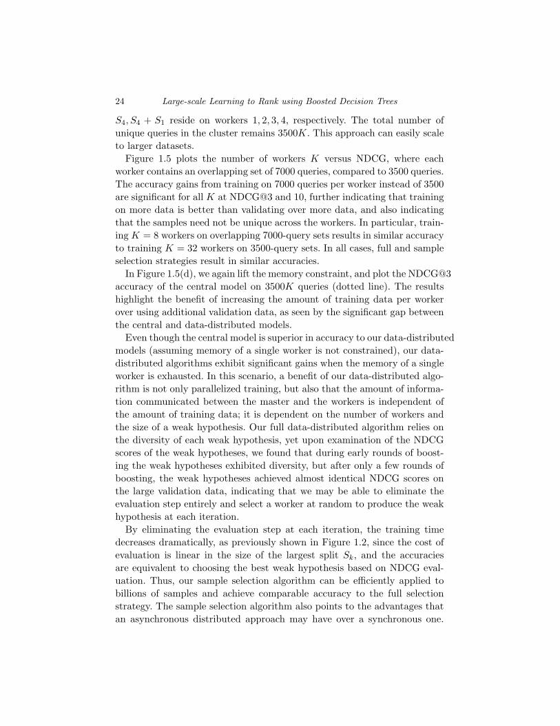
1.5 Number of Workers K versus NDCG@1, 3, 10 for full (solid) andsample (dashed) data-distributed LambdaMART. Each workertrains on 7000 overlapping queries (stars). Results from trainingon 3500 queries per worker (circles) are plotted for comparison.Figure (d) includes centralized LambdaMART (dotted) trainedon 3500K queries at each x-axis point. Signficant differences arestated in the text. 25

1.6 Number of Workers K vs. NDCG@1, 3, 10 for centralized (dot-

vi Illustrations

ted) and full (solid) and sample (dashed) data-distributed Lamb-

daMART. Each worker trains on |S|K

queries. The central model

was trained on |S|K

queries on a single worker. Significant differ-ences are stated in the text. 27

Tables

1.1 The learning rate η and the number of leaves L for central-ized LambdaMART, and full and sample data-distributed Lamb-daMART, respectively. The first set of columns are the param-eters when training on 3500 queries per worker; in the centralcase, a single worker trains on 3500K queries. The second set ofcolumns are the parameters when training on 7000 overlappingqueries per worker; in the central case, a single worker trains on7000K queries. The final columns contain the parameters when

training on |S|K

queries per worker; in the central case, a single

worker trains on |S|K

queries. 28

Contributors

Krysta M. Svore Microsoft Research, 1 Microsoft Way, Redmond, WA98052

Christopher J.C. Burges Microsoft Research, 1 Microsoft Way, Redmond,WA 98052

PART ONE

1

Large-scale Learning to Rank using BoostedDecision Trees

Krysta M. Svore and Christopher J.C. Burges

Abstract

The Web search ranking task has become increasingly important due to the

rapid growth of the internet. With the growth of the Web and the number

of Web search users, the amount of available training data for learning Web

ranking models has also increased. We investigate the problem of learning

to rank on a cluster using Web search data composed of 140,000 queries and

approximately fourteen million URLs. For datasets much larger than this,

distributed computing will become essential, due to both speed and memory

constraints. We compare to a baseline algorithm that has been carefully

engineered to allow training on the full dataset using a single machine, in

order to evaluate the loss or gain incurred by the distributed algorithms

we consider. The underlying algorithm we use is a boosted tree ranking

algorithm called LambdaMART, where a split at a given vertex in each

decision tree is determined by the split criterion for a particular feature. Our

contributions are two-fold. First, we implement a method for improving the

speed of training when the training data fits in main memory on a single

machine by distributing the vertex split computations of the decision trees.

The model produced is equivalent to the model produced from centralized

training, but achieves faster training times. Second, we develop a training

method for the case where the training data size exceeds the main memory

of a single machine. Our second approach easily scales to far larger datasets,

i.e., billions of examples, and is based on data distribution. Results of our

methods on a real-world Web dataset indicate significant improvements in

training speed.

4 Large-scale Learning to Rank using Boosted Decision Trees

1.1 Introduction

With the growth of the Web, large datasets are becoming increasingly com-

mon — a typical commercial search engine may gather several terabytes per

day of queries and Web search interaction information. This opens a wide

range of new opportunities, both because the best algorithm for a given

problem may change dramatically as more data becomes available (Banko

and Brill, 2001), and because such a wealth of data promises solutions to

problems that could not be previously approached. In addition, powerful

clusters of computers are becoming increasingly affordable. In light of these

developments, the research area of understanding how to most effectively

use both of these kinds of resources is rapidly developing. An example of a

goal in this area might be to train a Web search ranker on billions of doc-

uments, using user-clicks as labels, in a few minutes. Here, we concentrate

on training a Web search ranker on approximately fourteen million labeled

URLs, and our methods can scale to billions of URLs.

In this chapter, we investigate two synchronous approaches for learning to

rank on a distributed computer which target different computational scenar-

ios. In both cases, the base algorithm we use is LambdaMART (Wu et al.,

2009; Burges, 2010), which we describe in more detail below. LambdaMART

is a linear combination of regression trees, and as such lends itself to par-

allelization in various ways. Our first method applies when the full training

dataset fits in main memory on a single machine. In this case, our approach

distributes the tree split computations, but not the data. Note that while

this approach gives a speedup due to parallelizing the computation, it is

limited in the amount of data that can be used since all of the training data

must be stored in main memory on every node.

This limitation is removed in our second approach, which applies when

the full training dataset is too large to fit in main memory on a single

machine. In this case, our approach distributes the training data samples and

corresponding training computations and is scalable to very large amounts

of training data. We develop two methods of choosing the next regression

tree in the ensemble for our second approach, and compare and contrast

the resulting evaluation accuracy and training speed. In order to accurately

investigate the benefits and challenges of our techniques, we compare to a

standalone, centralized version that can train on the full training dataset

on a single node. To this end, the standalone version has been carefully

engineered (for example, memory usage is aggressively trimmed by using

different numbers of bits to encode different features).

Our primary contributions are:

1.2 Related Work 5

• A boosted decision tree ranking algorithm with the computations for de-

termining the best feature and value to split on at a given vertex in the

tree distributed across cluster nodes, designed to increase the speed of

training when the full training dataset fits in main memory. The model

produced is equivalent to the centralized counterpart, but the speed is

dramatically faster.

• A ranking algorithm with the training data and training computations

distributed, designed to exploit the full training dataset, and to yield

accuracy gains over training on the subset of training data that can be

stored in main memory on a single machine. The model produced is not

equivalent to the centralized counterpart. We assume in this case that a

single machine can only store a small subset of the entire training dataset,

and correspondingly assume that the centralized model cannot be trained

on all of the training data.

• An investigation of two techniques for selecting the next regression tree

in the ensemble.

• An investigation of using disjoint versus overlapping training datasets.

• A comprehensive study of the tradeoffs in speed and accuracy of our

distribution methods.

1.2 Related Work

There have been several approaches to distributed learning ranging from

data sampling to software parallelization. A survey of approaches is given

by Provost and Fayyad (1999). Many distributed learning techniques have

been motivated by the increasing size of datasets and their inability to fit

into main memory on a single machine. A distributed learning algorithm

produces a model that is either equivalent to the model produced by training

on the complete dataset on a single node, or comparable but not equivalent.

We first review previous work on algorithms where the output model is

equivalent. Caragea et al. (2004) present a general strategy for transforming

machine learning algorithms into distributed learning algorithms. They de-

termine conditions for which a distributed approach is better than a central-

ized approach in training time and communication time. In (van Uyen and

Chung, 2007), a synchronous, distributed version of AdaBoost is presented

where subsets of the data are distributed to nodes. Exact equivalence is ob-

tained by passing complete statistics about each sample to all other nodes.

In (Panda et al., 2009), a scalable approach to learning tree ensembles is

presented. The approach uses the MapReduce model (Dean and Ghemawat,


2004) and can run on commodity hardware. The split computations are dis-

tributed, rather than the data samples, and are converted into Map and

Reduce jobs. A challenge with the approach is that the communication cost

is linear in the number of training samples, which may lead to prohibitively

expensive communication costs for extremely large datasets.

The following distributed algorithms produce a model that is not equiv-

alent to the model produced from training on a centralized dataset. In

(Domingos and Hulten, 2000, 2001), learning algorithms, in particular K-

means clustering, are scaled to arbitrarily large datasets by minimizing the

number of data samples used at each step of the algorithm and by guaran-

teeing that the model is not significantly different from one obtained with

infinite data. The training speed improvements come from sampling the

training data; explicit distribution methods detailing communication costs

are not presented. Fan et al. (1999) present a distributed version of Ad-

aBoost, where each node contains a subset of the training data. During each

iteration, a classifier is built on a selected sample of training data. Two

sampling methods are examined: r -sampling, where a set of samples are

randomly chosen from the weighted training set, and d -sampling, where the

weighted training set is partitioned into disjoint subsets, and a given sub-

set is taken as a d -sample. After each round of boosting, the weights of all

training samples are updated according to a global weight vector. The speed

improvements are obtained through data sampling, while the communica-

tion cost scales with the number of training samples. The results indicate

that their approach is comparable to boosting over the complete data set

in only some cases. An extension of the work was developed in (Lazarevic,

2001; Lazarevic and Obradovic, 2002). Rather than add a classifier into the

ensemble built from a single disjoint d -sample or r -sample, classifiers built

from all distributed sites are combined into the ensemble. Several combi-

nation methods, including weighted voting and confidence-based weighting,

are considered. Experimental results indicate that accuracy is the same or

slightly better than boosting on centralized data. However, the large number

of classifiers combined to form the ensemble and the communication of the

global weight vector may be prohibitively expensive for practical use.

We present two methods of distributing LambdaMART. Our feature-

distributed method is similar to the approach in (Panda et al., 2009), except

that our method has a communication cost that is constant in the number

of training samples. Our data-distributed method differs from the previous

methods in that (1) we aim to produce a comparable, but not equivalent,

model, (2) we engineer our methods for a ranking task with billions of train-

ing samples, and (3) we use minimal communication cost that is constant

1.3 LambdaMART 7

in the number of training samples. Previous methods have required commu-

nication of global statistics to achieve both exact and approximate models,

and in each case the communication requirements scale with the number of

training samples. Since our second approach distributes by data sample, the

amount of training data (rather than the number of features) can scale with

cluster size, which is usually more desirable than scaling with the number of

features since the number of training samples tends to far exceed the number

of features. Each tree in the ensemble is trained using a small subset of the

data, and the best tree at a given iteration is chosen using the complement

of its training data as a validation set, so the model is well-regularized. In

the remainder of this chapter, we describe our experiences with developing a

distributed version of LambdaMART. We detail the benefits and challenges

of our two approaches, including the communication costs, training times,

and scalability to terabyte-size datasets.

1.3 LambdaMART

We use the LambdaMART algorithm for our boosted tree ranker (Wu et al.,

2009; Burges, 2010). LambdaMART combines MART (Friedman, 2001) and

LambdaRank (Burges et al., 2006; Burges, 2010). LambdaMART and Lamb-

daRank were the primary components of the winning ranking system in the

recent Yahoo! Learning to Rank Challenge for Web search (Yahoo! Learn-

ing to Rank Challenge, 2010; Burges et al., 2011). We briefly describe these

algorithms here.

LambdaRank is a general method for learning to rank given an arbitrary

cost function, and it circumvents the problem that most information retrieval

measures have ill-posed gradients. It has been shown empirically that Lamb-

daRank can optimize general IR measures (Donmez et al., 2009). A key idea

in LambdaRank is to define the derivatives (of the cost with respect to the

model scores) after the documents have been sorted by the current model

scores, which circumvents the problem of defining a derivative of a mea-

sure whose value depends on the sorted order of a set of documents. These

derivatives are called λ-gradients. A second key observation in LambdaRank

is to note that many training algorithms (for example, neural network train-

ing and MART) do not need to know the cost directly; they only need the

derivatives of the cost with respect to the model scores.

For example, the λ-gradient for NDCG (Jarvelin and Kekalainen, 2000)

for a pair of documents Di and Dj , where Di is more relevant to query q

than Dj , can be defined as the product of the derivative of a convex cost


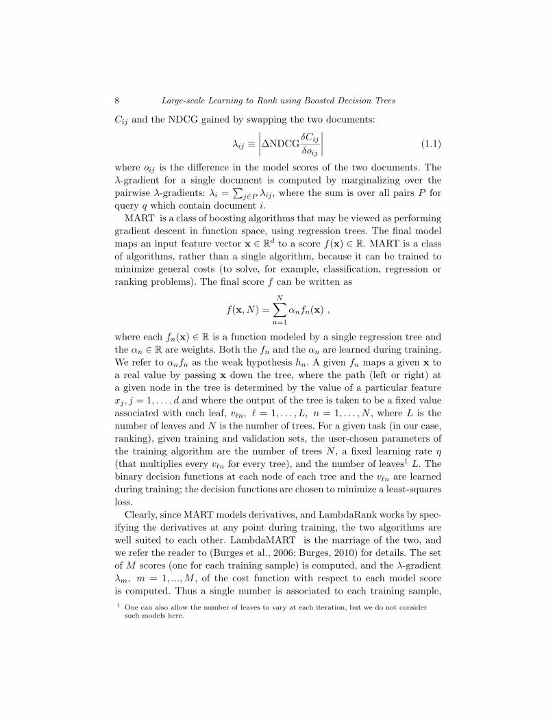
Cij and the NDCG gained by swapping the two documents:

λij ≡

∣

∣

∣

∣

∆NDCGδCij

δoij

∣

∣

∣

∣

(1.1)

where oij is the difference in the model scores of the two documents. The

λ-gradient for a single document is computed by marginalizing over the

pairwise λ-gradients: λi =∑

j∈P λij , where the sum is over all pairs P for

query q which contain document i.

MART is a class of boosting algorithms that may be viewed as performing

gradient descent in function space, using regression trees. The final model

maps an input feature vector x ∈ Rd to a score f(x) ∈ R. MART is a class

of algorithms, rather than a single algorithm, because it can be trained to

minimize general costs (to solve, for example, classification, regression or

ranking problems). The final score f can be written as

f(x, N) =N

∑

n=1

αnfn(x) ,

where each fn(x) ∈ R is a function modeled by a single regression tree and

the αn ∈ R are weights. Both the fn and the αn are learned during training.

We refer to αnfn as the weak hypothesis hn. A given fn maps a given x to

a real value by passing x down the tree, where the path (left or right) at

a given node in the tree is determined by the value of a particular feature

xj , j = 1, . . . , d and where the output of the tree is taken to be a fixed value

associated with each leaf, vℓn, ℓ = 1, . . . , L, n = 1, . . . , N , where L is the

number of leaves and N is the number of trees. For a given task (in our case,

ranking), given training and validation sets, the user-chosen parameters of

the training algorithm are the number of trees N , a fixed learning rate η

(that multiplies every vℓn for every tree), and the number of leaves1 L. The

binary decision functions at each node of each tree and the vℓn are learned

during training; the decision functions are chosen to minimize a least-squares

loss.

Clearly, since MART models derivatives, and LambdaRank works by spec-

ifying the derivatives at any point during training, the two algorithms are

well suited to each other. LambdaMART is the marriage of the two, and

we refer the reader to (Burges et al., 2006; Burges, 2010) for details. The set

of M scores (one for each training sample) is computed, and the λ-gradient

λm, m = 1, ..., M , of the cost function with respect to each model score

is computed. Thus a single number is associated to each training sample,

1 One can also allow the number of leaves to vary at each iteration, but we do not considersuch models here.

1.3 LambdaMART 9

namely, the gradient of the cost with respect to the score which the model

assigns to that sample. Tree fn is then just a least-squares regression tree

that models this set of gradients (so each leaf models a single value of the

gradient). The overall cost is then reduced by taking a step along the gra-

dient. This is often done by computing a Newton step vℓn for each leaf,

where the vℓn can be computed exactly for some costs. Every leaf value is

then multiplied by a learning rate η. Taking a step that is smaller than the

optimal step size (i.e., the step size that is estimated to maximally reduce

the cost) acts as a form of regularization for the model that can significantly

improve test accuracy. The LambdaMART algorithm is outlined in Algo-

rithm 1, where we have added the notion that the first model trained can be

any previously trained model (Step 3), which is useful for model adaptation

tasks.

Algorithm 1 LambdaMART.

1: Input: Training Data: {xm, ym}, m = 1, . . . , M ;

Number of Trees: N ;

Number of Leaves: L;

Learning Rate: η;

2: Output: Model: f(x, N);

3: f(x, 0) = BaseModel(x) {BaseModel may be empty.}

4: for n = 1 to N do

5: for m = 1 to M do

6: λm = G(q,x, y, m) {Calculate λ-gradient for sample m as a function

of the query q and the documents and labels x, y associated with

q.}

7: wm = ∂λm

∂f(xm) {Calculate derivative of λ-gradient for sample m.}

8: end for

9: {Rℓn}Lℓ=1 {Create L-leaf regression tree on {xm, λm}M

m=1.}

10: for ℓ = 1 to L do

11: vℓn =

P

xm∈Rℓnλm

P

xm∈Rℓnwm

{Find the leaf values based on approximate New-

ton step.}

12: end for

13: f(xm, n) = f(xm, n−1)+η∑

ℓ vℓn1(xm ∈ Rℓn) {Update model based

on approximate Newton step and learning rate.}

14: end for


1.4 Approaches to Distributing LambdaMART

As previously noted, we focus on the task of ranking, in particular Web

search ranking, by learning boosted tree ensembles produced using Lamb-

daMART. This means that the final model f is an ensemble defined as the

sum f(x, N) =∑N

n=1 hn(x), where each hn is a weak hypothesis. Moreover,

f is constructed incrementally as weak hypotheses are added one by one.

In this section, we present two approaches for distributed learning using

LambdaMART:

1. Our first approach attempts to decrease training time by distributing

the vertex split computations across the nodes and results in a solution

which is equivalent to the solution resulting from training on all of the

data on a single node (called the centralized model). We call this approach

feature-distributed LambdaMART.

2. Our second approach distributes the training data across the nodes and

does not produce a model equivalent to the centralized model. Rather,

it attempts to dramatically reduce communication requirements without

sacrificing accuracy and yields the possibility of training on billions of

samples. We call this approach data-distributed LambdaMART. Within

our second approach, we consider two weak hypothesis selection methods:

• the master picks the weak hypothesis that maximizes the evaluation

score (referred to as full selection)

• the master picks a weak hypothesis at random, in order to decrease

communication costs (referred to as sample selection)

Throughout the chapter, we assume that our distributed computer (clus-

ter) has K + 1 nodes, one of which may be designated as master, while the

others are workers. We denote the workers by W1, . . . , WK and use [K] to

denote the set {1, . . . , K}.

1.4.1 A Synchronous Approach based on Feature Distribution

In this section, we present feature-distributed LambdaMART, a synchronous

distributed algorithm similar to the approach in (Panda et al., 2009) that

distributes the vertex split computations in the boosted decision trees. Our

method differs from that in (Panda et al., 2009) since the communication

cost of our method is constant in the number of training samples (as opposed

to linear). In addition, our method is based on MPI communication and does

not use the Map-Reduce framework.

Recall that this approach targets the scenario where each node can store


the full training dataset in main memory. Due to extensive engineering and

optimization, we have been able to store a dataset with several thousand

features and over fourteen million samples in main memory on a single ma-

chine. Our goal is to train on such a large dataset on a cluster more quickly

than on a single machine, while outputting the same model as the centralized

counterpart.

Our algorithm, detailed in Algorithm 2, proceeds as follows. Let there be

K workers and no master. We are given a training set S of M instance-label

pairs. Each node stores the full training set S in memory. Let A be the set of

features. The features are partitioned into K subsets, A1, . . . , AK , such that

each subset is assigned to one of the K workers. Every worker maintains a

copy of the ensemble f(x, n) and updates it after each boosting iteration n.

During each boosting iteration, a regression tree {Rℓn}Lℓ=1 is constructed.

Each vertex in the tree is described by an optimal feature, corresponding

split threshold, and change in loss, collectively denoted by ϕ. Each worker k

computes the optimal feature and corresponding split threshold among its

set of features Ak and sends the optimal feature, threshold, and change in

loss, denoted by ϕk, to all other workers.

Every worker, after it has received all of the ϕk’s, determines the ϕk with

the smallest loss, denoted by ϕ∗, creates the two new children for the model,

and then computes which samples go left and which go right. Note that ϕ∗

is the same for all workers, resulting in equivalent ensembles f(x, n) across

all workers. The algorithm is synchronized as follows: each worker must wait

until it receives all ϕk, k = 1, . . . , K, before determining ϕ∗. Some workers

will be idle while others are still computing their ϕk’s.

The challenge of this approach is that it requires that every worker contain

a copy of the full training dataset. A benefit is the corresponding reduction

in communication: each worker only sends a limited amount of information

about a single feature for each vertex split computation. The total commu-

nication cost depends on the number of leaves L in a tree and the number

of workers K in the cluster, but does not depend on the number of training

samples or on the number of features.

1.4.2 A Synchronous Approach based on Data Distribution

Previous techniques of distributed boosted tree learning have focused on

producing an ensemble that is equivalent to the ensemble produced by cen-

tralized training (Caragea et al., 2004; van Uyen and Chung, 2007; Panda

et al., 2009). These approaches require that sufficient global statistics of the

data be communicated among the master and the workers. Let there be


Algorithm 2 Feature-distributed LambdaMART.

1: Input: Training Data: {xm, ym}, m = 1, · · · , M ;



Learning Rate: η;

Number of Workers: K;


3: for k = 1 to K do



6: for m = 1 to M do

7: λm = G(q,x, y, m) {Calculate λ-gradient for sample m as a func-

tion of the query q and the documents and labels x, y associated

with q.}

8: wm = ∂λm


9: end for

10: for ℓ = 1 to L − 1 do

11: ϕk {Compute the optimal feature and split, ϕk, over features Ak

on worker k.}

12: Broadcast(ϕk) {Broadcast ϕk to all other workers.}

13: ϕ∗ = {arg maxk(ϕk)}Kk=1 {Find optimal ϕ∗ across all ϕk’s.}

14: Rℓn {Create regression tree on ϕ∗ and {xm, λm}Mm=1.}

15: end for


17: vℓn =

P

xm∈Rℓnλm

P

xm∈Rℓnwℓ

{Find the leaf values based on approximate

Newton step.}

18: end for

19: f(xm, n) = f(xm, n − 1) + η∑

ℓ vℓn1(xm ∈ Rℓn) {Update model

based on approximate Newton step and learning rate.}

20: end for

21: end for

a single master and K workers. The training set S is partitioned into K

subsets, S1, . . . , SK , and each subset resides on one of the workers of our

distributed computer. For simplicity, assume that the subsets are equal in

size, although this is not required in our derivation. However, we make no

assumptions on how S is split, and specifically we do not require the subsets

to be statistically equivalent.

Let data subset Sk reside on node k. To achieve a model equivalent to


the centralized model, we could, for each vertex in the tree, send from each

worker k to the master the split information for each feature, which includes

which samples in Sk go left or right when split on that feature. The master

then determines the best feature and split values based on S. In this case,

the communication cost per regression tree is dependent on the number of

vertices in the tree, the range of split values considered, the number of fea-

tures, and the number of data samples. The communication resources per

vertex have a linear dependence on the number of training samples, preclud-

ing the use of the approach when the number of samples is in the billions. We

would like to devise an algorithm that achieves comparable accuracy, but

requires far less communication resources, namely, a communication cost

that is independent of the number of training samples. We now describe our

approach.

Assume that we have already performed N −1 iterations of our algorithm

and therefore the master already has an ensemble f(x, N − 1) composed of

N − 1 weak hypotheses. The task is now to choose a new weak hypothesis

to add to the ensemble. Each worker has a copy of f(x, N − 1) and uses its

portion of the data to train a candidate weak hypothesis. Namely, worker k

uses ensemble f(x, N − 1) and dataset Sk to generate the weak hypothesis

hN,k(x) and sends it to all other workers.

Each worker now evaluates all of the candidates constructed by the other

workers. Namely, worker k evaluates the set {hN,k(x)}[K]\{k}, where fk(x, N) =

f(x, N −1)+hN,k(x), and calculates the set of values {Ck(fk(x, N))}[K]\{k}

and returns these values to the master, where C is the evaluation measure.

The master then chooses the candidate with the largest evaluation score

C on the entire training set S. This step of cross-validation adds a further

regularization component to the training. We call this method the full selec-

tion method. Letting V denote the set of indices of candidates, the master

calculates

C(fk(x, N)) =∑

i∈V

Ci(fk(x, N)) ,

for each candidate k. Finally, the master chooses the candidate with the

largest average score, and sets

f(x, N) = argmaxfk(x,N)

C(fk(x, N)) .

The master sends the index k of the selected weak hypothesis to all workers.

Each worker then updates the model: f(x, N) = f(x, N − 1) + hN,k(x). On

the next iteration, all of the workers attempt to add another weak learner

to f(x, N).


The intuition behind our approach is that if the hypotheses are sufficiently

diverse, then the hypotheses will exhibit dramatically different evaluation

scores. The cross-validation ideally results in an ensemble of weak hypotheses

that is highly regularized; we test this hypothesis through experiments in

Section 1.5.

The communication cost of our approach is dependent on the size of the

weak hypothesis and the number of workers, but is not dependent on the

size of the training data. In addition, communication only occurs once per

boosting iteration, removing the need to communicate once per vertex split

computation. Each weak hypothesis must be communicated to all other

workers, and the resulting evaluation scores must be communicated from

each worker to the master. Essentially, the scores are an array of doubles,

where the length of the array is the number of weak hypotheses evaluated.

Once the master has determined the best weak hypothesis to add to the

ensemble, the master need only communicate the index of the best model

back to the workers. Each worker updates its model accordingly.

1.4.3 Adding Randomization

The straightforward data-distributed approach presented in Section 1.4.2

has the workers performing two different types of tasks: constructing can-

didate weak hypotheses and evaluating candidate ensembles that were con-

structed by others. If the training data size is fixed, and as the number of

workers K increases, each worker trains on a smaller portion of the training

data, namely |S|K

, then the task of constructing candidates can be completed

faster. On the other hand, assuming that evaluation time is linear in the

number of samples, the total time spent evaluating other candidates stays

roughly constant. To see this, note that each worker has to evaluate K − 1

candidates on |S|K

samples, for a total evaluation time on the order of |S|K−1K

.

To resolve this problem, we need to reduce the number of evaluations; we

accomplish this using the power of sampling. We call this method the sample

selection method.

The algorithm proceeds as before: all of the workers are given the same

ensemble f(x, N −1) and use their datasets to construct candidates. Worker

k constructs fk(x, N). Rather than the master receiving K candidate weak

hypotheses, it chooses a random worker k among the set and the chosen

worker communicates hN,k(x) to all other workers (replacing Steps 15–17 in

Algorithm 3 with random selection of a hypothesis). The randomized selec-

tion of a candidate removes the need for extensive evaluation and requires

only communicating the chosen candidate weak hypothesis from the master


Algorithm 3 Data-distributed LambdaMART.

1: Input: Training Data: {xm, ym}, m = 1, . . . , M ;



Learning Rate: η;

Number of Workers: K;


3: for k = 1 to K do



6: for all m ∈ Sk do

7: λm = G(q,x, y, m) {Calculate λ-gradient for sample m as a func-

tion of the query q and the documents and labels x, y associated

with q, where m is in the fraction of training data Sk on worker

k.}

8: wm = ∂λm


9: end for

10: {Rℓn}Lℓ=1 {Create L-leaf regression tree {Rℓnk}

Lℓ=1 on

{xm, λm}, m ∈ Sk.}


12: vℓn =

P

xm∈Rℓnλm

P

xm∈Rℓnwm

{Find the leaf values based on approximate

Newton step.}

13: end for

14: fk(xm, n) = f(xm, n − 1) + η∑

ℓ vℓn1(xm ∈ Rℓnk) {Update model

based on approximate Newton step and learning rate.}

15: {Ck(fk(x, n))}[K]\{k} {Compute candidate weak hypotheses cost

values.}

16: C(fk(x, n)) =∑

i∈V Ci(fk(x, n)) {Evaluate candidate weak hy-

potheses from all other workers.}

17: f(x, n) = argmaxfk(x,n)

C(fk(x, n)) {Choose best weak hypothesis and

update model.}

18: end for

19: end for

to the workers. This rough estimate may be enough to offer additional regu-

larization over always choosing the same data sample to construct the weak

hypothesis. It eliminates the expensive evaluation step previously required


for each candidate at each boosting iteration in the full selection method

and will work well if the hypotheses in fact exhibit very little diversity.

1.5 Experiments

In this section, we evaluate our proposed methods on a real-world Web

dataset. We ran all of our experiments on a 40-node MPI cluster, running

Microsoft HPC Server 2008. One node serves as the cluster scheduler, and the

remaining 39 are compute nodes. Each node has two 4-core Intel Xeon 5550

processors running at 2.67GHz and 48 GB of RAM. Each node is connected

to two 1Gb Ethernet networks: a private network dedicated to MPI traffic

and a public network. Each network is provided by a Cisco 3750e Ethernet

switch. The communication layer between nodes on our cluster was written

using MPI.NET.

Total train time was measured as the time in seconds between the com-

pletion of the loading of the data on the cluster nodes and the completion

of the final round of boosting. The time does not include loading data or

testing the final model. To mitigate effects of varying cluster conditions, we

ran each experimental setting three times and plot all three values.

We swept a range of parameter values for each experiment: we varied the

learning rate η from 0.05 to 0.5 and the number of leaves L from 20 to

220, and trained for N = 1000 boosting iterations. We determined the best

iteration and set of parameter values based on the evaluation accuracy of

the model on a validation set.

1.5.1 Data

Our real-world Web data collection contains queries sampled from query

log files of a commercial search engine and corresponding URLs. All queries

are English queries and contain up to 10 query terms. We perform some

stemming on queries. Each query is associated with on average 150–200

documents (URLs), each with a vector of several thousand feature values

extracted for the query-URL pair and a human-generated relevance label

l ∈ {0, 1, 2, 3, 4}, with 0 meaning document d is not relevant to query q and

4 meaning d is highly relevant to q. The dataset contains 140,000 queries and

corresponding URLs (14,533,212 query-URL pairs). We refer to the dataset

size in terms of the number queries, where an n-query dataset means a

dataset consisting of all query-URL pairs for those n queries.

We divide the dataset into train, valid, and test sets by selecting a random

80% of samples for training, a random 10% for validation, and a random 10%

1.5 Experiments 17

for test. We require that for a given query, all corresponding URLs (samples)

reside in the same data split. In some experiments, we reduce the amount

of training data by 1k, k = {2, 4, 8, 16, 32}. The resulting change in accuracy

will indicate the sensitivity of the algorithms to the training data size.

1.5.2 Evaluation Measure

We evaluate using NDCG, Normalized Discounted Cumulative Gain (NDCG)

(Jarvelin and Kekalainen, 2000), a widely used measure for search metrics.

It operates on multilevel relevance labels; in our work, relevance is measured

on a 5-level scale. NDCG for a given query q is defined as follows:

NDCG@T (q) =100

Z

T∑

r=1

2l(r) − 1

log(1 + r)(1.2)

where l(r) ∈ {0, . . . , 4} is the relevance label of the document at rank posi-

tion r and T is the truncation level to which NDCG is computed. Z is cho-

sen such that the perfect ranking would result in NDCG@T (q) = 100. Mean

NDCG@T is the normalized sum over all queries: 1Q

∑Qq=1 NDCG@T (q).

NDCG is particularly well-suited for Web search applications since it ac-

counts for multilevel relevance labels and the truncation level can be set

to model user behavior. In our studies, we evaluate our results using mean

NDCG@1, 3, 10. For brevity, we write NDCG@1, 3, 10. We also perform a

signficance t-test with a significance level of 0.05. A significant difference

should be read as significant at the 95% confidence level. All accuracy re-

sults are reported on the same 14K-query test set.

1.5.3 Time Complexity Comparison

We first examine the speed improvements and communication requirements

of our distributed LambdaMART algorithms compared to the centralized

LambdaMART algorithm. A major advantage of training a distributed learn-

ing algorithm over a centralized learning algorithm, in addition to being able

to take advantage of more data, is the decrease in training time.

The total training time complexities of centralized LambdaMART, feature-

distributed LambdaMART, and data-distributed LambdaMART are O(|S||A|),

O(|S||Ak|), and O(|Sk||A|), respectively, where |S| is the size of the train-

ing data, |A| is the number of features, and k indexes the node. Sample

data-distributed LambdaMART requires only a constant additional com-

munication cost and no evaluation cost. When the number of features is


large, the feature-distributed algorithm is significantly more efficient than

the centralized algorithm. When |A| ≪ |S|, which is commonly the case, the

sample data-distributed algorithm is significantly more efficient than both

the centralized and feature-distributed algorithms.

Figures 1.1(a)–(d) show the difference in total training time between cen-

tralized LambdaMART and feature-distributed LambdaMART. We vary the

number of workers K from 1–32, and the number of features |A| from 500–

4000. For feature-distributed LambdaMART, |A|K

features are assigned to

each node. We employ the same set of parameters for each algorithm to

provide fair training time comparisons; the parameters are set to η = 0.1,

N = 500, and L = 200. We evaluated the total train time of feature-

distributed LambdaMART on two types of clusters. The first cluster is as

previously described, and we denote it as Type I. Each node in the second

cluster, denoted as Type II, has 32.0 GB RAM and two quad-core Intel Xeon

5430 processors running at 2.67 GHz.

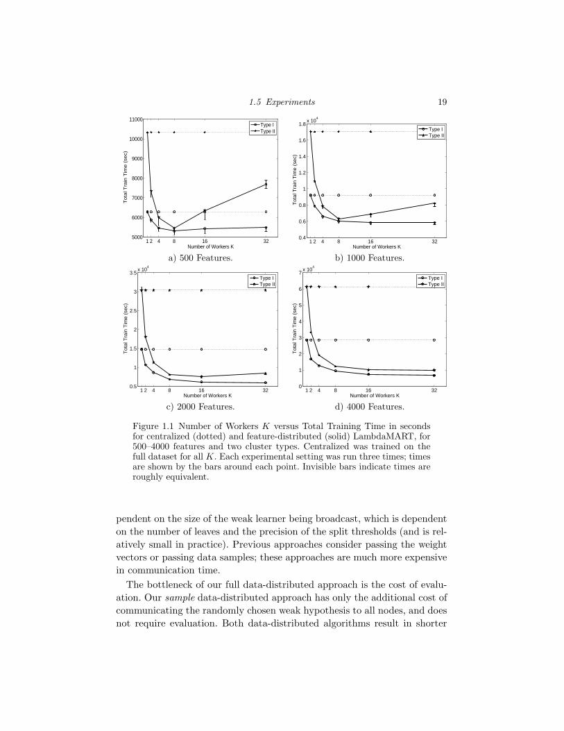
As shown in Figure 1.1, feature-distributed LambdaMART (solid lines)

achieves significantly faster training times than centralized LambdaMART

(dotted lines) on both clusters. When trained on Type II with 500 fea-

tures, feature-distributed LambdaMART with 8 workers achieves almost a

two-fold speed-up over centralized LambdaMART (Fig. 1.1(a)). When the

number of features is small, as the number of workers increases, the cost

of communication among the workers outweighs the speed-ups due to fea-

ture distribution, as seen by the increase in time when K ≥ 8 for Type II

(Fig. 1.1(a)–(b)). However, as the number of features increases, communica-

tion occupies a smaller percentage of the training time, resulting in decreas-

ing training times. For example, feature-distributed LambdaMART on Type

II with 4000 features (Fig. 1.1(d)) exhibits decreasing training times as the

number of workers increases and achieves a factor of 6 speed-up over cen-

tralized LambdaMART when trained on 32 workers. When trained on Type

I, feature-distributed LambdaMART exhibits decreasing training times as

the number of workers grows; with 32 workers training on 4000 features,

roughly a 3-fold speed-up is obtained.

Our full data-distributed algorithm incurs an additional cost for the eval-

uation of weak hypotheses and the communication of the evaluation results

and the chosen weak hypothesis. The evaluation cost is linear in the number

of training samples |S|, but unlike previous methods, the communication

cost is independent of the number of training samples, therefore network

communication is not a bottleneck as |S| increases to billions of samples.

The communication cost scales linearly with the number of nodes and is de-

1.5 Experiments 19

1 2 4 8 16 325000

6000

7000

8000

9000

10000

11000

Number of Workers K

Tota

l Tra

in T

ime (

sec)

Type IType II

1 2 4 8 16 320.4

0.6

0.8

1

1.2

1.4

1.6

1.8x 10

4

Number of Workers K

Tot

al T

rain

Tim

e (s

ec)

Type IType II

a) 500 Features. b) 1000 Features.

1 2 4 8 16 320.5

1

1.5

2

2.5

3

3.5x 10

4

Number of Workers K

Tot

al T

rain

Tim

e (s

ec)

Type IType II

1 2 4 8 16 320

1

2

3

4

5

6

7x 10

4

Number of Workers K

Tot

al T

rain

Tim

e (s

ec)

Type IType II

c) 2000 Features. d) 4000 Features.

Figure 1.1 Number of Workers K versus Total Training Time in secondsfor centralized (dotted) and feature-distributed (solid) LambdaMART, for500–4000 features and two cluster types. Centralized was trained on thefull dataset for all K. Each experimental setting was run three times; timesare shown by the bars around each point. Invisible bars indicate times areroughly equivalent.

pendent on the size of the weak learner being broadcast, which is dependent

on the number of leaves and the precision of the split thresholds (and is rel-

atively small in practice). Previous approaches consider passing the weight

vectors or passing data samples; these approaches are much more expensive

in communication time.

The bottleneck of our full data-distributed approach is the cost of evalu-

ation. Our sample data-distributed approach has only the additional cost of

communicating the randomly chosen weak hypothesis to all nodes, and does

not require evaluation. Both data-distributed algorithms result in shorter


training times than the centralized algorithm since the training data per

worker k is smaller, |S|k

.

Figure 1.2 shows the number of workers versus the total training time in

seconds, for weak hypotheses with varying numbers of leaves, for centralized,

and full and sample data-distributed LambdaMART. The same parameter

settings are used for the three approaches: L = 20, N = 1000, and η = 0.1.

The x-axis indicates the number of workers K, where each worker trains

on |S|32 ≈ 3500 queries; with respect to centralized LambdaMART, the x-

axis indicates the number of training queries residing on the single worker,|S|32 K. The point at K = 1 represents training centralized LambdaMART

1 2 4 8 16 320

2500

5000

7500

10000

12500

15000

Number of Workers K

Tota

l Tra

in T

ime (

sec)

Figure 1.2 Number of Workers K: total data used = 3500K queries ver-sus Training Time in seconds for centralized (dotted), full data-distributed(solid), and sample data-distributed (dashed) LambdaMART with L = 20leaves. Each experimental setting was run three times; times are shownby the bars around each point. Invisible bars indicate times are roughlyequivalent.

on |S|32 ≈ 3500 queries. As K increases, the total train time increases since

the communication costs grow with the number of workers K. Since the

evaluation and communication costs are almost negligible in sample data-

distributed LambdaMART, the total train time is roughly equivalent to

training on a single node, even though the amount of training data across

the cluster increases with K.

We next evaluate the time required to train on |S| queries, where the

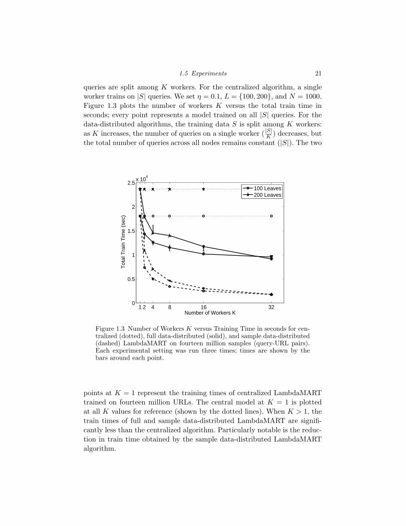
1.5 Experiments 21

queries are split among K workers. For the centralized algorithm, a single

worker trains on |S| queries. We set η = 0.1, L = {100, 200}, and N = 1000.

Figure 1.3 plots the number of workers K versus the total train time in

seconds; every point represents a model trained on all |S| queries. For the

data-distributed algorithms, the training data S is split among K workers:

as K increases, the number of queries on a single worker ( |S|K

) decreases, but

the total number of queries across all nodes remains constant (|S|). The two

1 2 4 8 16 320

0.5

1

1.5

2

2.5x 10

4

Number of Workers K

Tot

al T

rain

Tim

e (s

ec)

100 Leaves200 Leaves

Figure 1.3 Number of Workers K versus Training Time in seconds for cen-tralized (dotted), full data-distributed (solid), and sample data-distributed(dashed) LambdaMART on fourteen million samples (query-URL pairs).Each experimental setting was run three times; times are shown by thebars around each point.

points at K = 1 represent the training times of centralized LambdaMART

trained on fourteen million URLs. The central model at K = 1 is plotted

at all K values for reference (shown by the dotted lines). When K > 1, the

train times of full and sample data-distributed LambdaMART are signifi-

cantly less than the centralized algorithm. Particularly notable is the reduc-

tion in train time obtained by the sample data-distributed LambdaMART

algorithm.


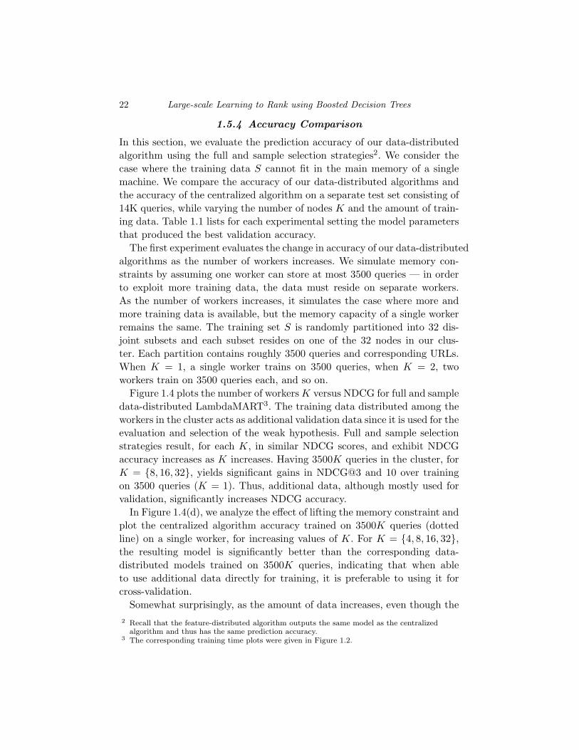
1.5.4 Accuracy Comparison

In this section, we evaluate the prediction accuracy of our data-distributed

algorithm using the full and sample selection strategies2. We consider the

case where the training data S cannot fit in the main memory of a single

machine. We compare the accuracy of our data-distributed algorithms and

the accuracy of the centralized algorithm on a separate test set consisting of

14K queries, while varying the number of nodes K and the amount of train-

ing data. Table 1.1 lists for each experimental setting the model parameters

that produced the best validation accuracy.

The first experiment evaluates the change in accuracy of our data-distributed

algorithms as the number of workers increases. We simulate memory con-

straints by assuming one worker can store at most 3500 queries — in order

to exploit more training data, the data must reside on separate workers.

As the number of workers increases, it simulates the case where more and

more training data is available, but the memory capacity of a single worker

remains the same. The training set S is randomly partitioned into 32 dis-

joint subsets and each subset resides on one of the 32 nodes in our clus-

ter. Each partition contains roughly 3500 queries and corresponding URLs.

When K = 1, a single worker trains on 3500 queries, when K = 2, two

workers train on 3500 queries each, and so on.

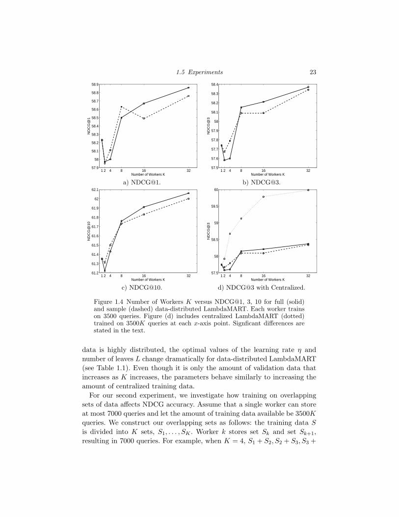
Figure 1.4 plots the number of workers K versus NDCG for full and sample

data-distributed LambdaMART3. The training data distributed among the

workers in the cluster acts as additional validation data since it is used for the

evaluation and selection of the weak hypothesis. Full and sample selection

strategies result, for each K, in similar NDCG scores, and exhibit NDCG

accuracy increases as K increases. Having 3500K queries in the cluster, for

K = {8, 16, 32}, yields significant gains in NDCG@3 and 10 over training

on 3500 queries (K = 1). Thus, additional data, although mostly used for

validation, significantly increases NDCG accuracy.

In Figure 1.4(d), we analyze the effect of lifting the memory constraint and

plot the centralized algorithm accuracy trained on 3500K queries (dotted

line) on a single worker, for increasing values of K. For K = {4, 8, 16, 32},

the resulting model is significantly better than the corresponding data-

distributed models trained on 3500K queries, indicating that when able

to use additional data directly for training, it is preferable to using it for

cross-validation.

Somewhat surprisingly, as the amount of data increases, even though the

2 Recall that the feature-distributed algorithm outputs the same model as the centralizedalgorithm and thus has the same prediction accuracy.

3 The corresponding training time plots were given in Figure 1.2.

1.5 Experiments 23

1 2 4 8 16 3257.9

58

58.1

58.2

58.3

58.4

58.5

58.6

58.7

58.8

58.9N

DC

G@

1

Number of Workers K1 2 4 8 16 32

57.5

57.6

57.7

57.8

57.9

58

58.1

58.2

58.3

58.4

ND

CG

@3

Number of Workers K

a) NDCG@1. b) NDCG@3.

1 2 4 8 16 3261.2

61.3

61.4

61.5

61.6

61.7

61.8

61.9

62

62.1

ND

CG

@10


57.5

58

58.5

59

59.5

60

ND

CG

@3

Number of Workers K

c) NDCG@10. d) NDCG@3 with Centralized.

Figure 1.4 Number of Workers K versus NDCG@1, 3, 10 for full (solid)and sample (dashed) data-distributed LambdaMART. Each worker trainson 3500 queries. Figure (d) includes centralized LambdaMART (dotted)trained on 3500K queries at each x-axis point. Signficant differences arestated in the text.

data is highly distributed, the optimal values of the learning rate η and

number of leaves L change dramatically for data-distributed LambdaMART

(see Table 1.1). Even though it is only the amount of validation data that

increases as K increases, the parameters behave similarly to increasing the

amount of centralized training data.

For our second experiment, we investigate how training on overlapping

sets of data affects NDCG accuracy. Assume that a single worker can store

at most 7000 queries and let the amount of training data available be 3500K

queries. We construct our overlapping sets as follows: the training data S

is divided into K sets, S1, . . . , SK . Worker k stores set Sk and set Sk+1,

resulting in 7000 queries. For example, when K = 4, S1 + S2, S2 + S3, S3 +


S4, S4 + S1 reside on workers 1, 2, 3, 4, respectively. The total number of

unique queries in the cluster remains 3500K. This approach can easily scale

to larger datasets.

Figure 1.5 plots the number of workers K versus NDCG, where each

worker contains an overlapping set of 7000 queries, compared to 3500 queries.

The accuracy gains from training on 7000 queries per worker instead of 3500

are significant for all K at NDCG@3 and 10, further indicating that training

on more data is better than validating over more data, and also indicating

that the samples need not be unique across the workers. In particular, train-

ing K = 8 workers on overlapping 7000-query sets results in similar accuracy

to training K = 32 workers on 3500-query sets. In all cases, full and sample

selection strategies result in similar accuracies.

In Figure 1.5(d), we again lift the memory constraint, and plot the NDCG@3

accuracy of the central model on 3500K queries (dotted line). The results

highlight the benefit of increasing the amount of training data per worker

over using additional validation data, as seen by the significant gap between

the central and data-distributed models.

Even though the central model is superior in accuracy to our data-distributed

models (assuming memory of a single worker is not constrained), our data-

distributed algorithms exhibit significant gains when the memory of a single

worker is exhausted. In this scenario, a benefit of our data-distributed algo-

rithm is not only parallelized training, but also that the amount of informa-

tion communicated between the master and the workers is independent of

the amount of training data; it is dependent on the number of workers and

the size of a weak hypothesis. Our full data-distributed algorithm relies on

the diversity of each weak hypothesis, yet upon examination of the NDCG

scores of the weak hypotheses, we found that during early rounds of boost-

ing the weak hypotheses exhibited diversity, but after only a few rounds of

boosting, the weak hypotheses achieved almost identical NDCG scores on

the large validation data, indicating that we may be able to eliminate the

evaluation step entirely and select a worker at random to produce the weak

hypothesis at each iteration.

By eliminating the evaluation step at each iteration, the training time

decreases dramatically, as previously shown in Figure 1.2, since the cost of

evaluation is linear in the size of the largest split Sk, and the accuracies

are equivalent to choosing the best weak hypothesis based on NDCG eval-

uation. Thus, our sample selection algorithm can be efficiently applied to

billions of samples and achieve comparable accuracy to the full selection

strategy. The sample selection algorithm also points to the advantages that

an asynchronous distributed approach may have over a synchronous one.

1.5 Experiments 25

1 2 4 8 16 3258

58.2

58.4

58.6

58.8

59

59.2

59.4N

DC

G@

1


57.6

57.8

58

58.2

58.4

58.6

58.8

59

ND

CG

@3

Number of Workers K


1 2 4 8 16 3261.4

61.5

61.6

61.7

61.8

61.9

62

62.1

62.2

62.3

62.4

ND

CG

@10


57.5

58

58.5

59

59.5

60

ND

CG

@3

Number of Workers K

c) NDCG@10. d) NDCG@3 with Centralized.

Figure 1.5 Number of Workers K versus NDCG@1, 3, 10 for full (solid) andsample (dashed) data-distributed LambdaMART. Each worker trains on7000 overlapping queries (stars). Results from training on 3500 queries perworker (circles) are plotted for comparison. Figure (d) includes centralizedLambdaMART (dotted) trained on 3500K queries at each x-axis point.Signficant differences are stated in the text.

Since each worker k trains on a random subset Sk of the training data, then

an asynchronous algorithm could assign idle workers different tasks, such

as evaluating or training a regression tree for a future iteration. Such an

approach could possibly yield improvements in speed or accuracy by taking

advantage of the large number of workers available at any given time.

Our sample approach can also be applied to centralized training: at each

round of boosting, sample the training data and train a weak hypothesis

on that sample. If the complete training dataset fits in memory on a single

machine, then the training time will decrease by training on a sample of

the data during each boosting iteration. However, if the training data must


reside on separate machines, then to train on a single machine, at each

round of boosting, the sample must be sent to the machine and then loaded

into memory on the machine. The sample must be sampled across all of the

machines. The process of communicating the data samples from the many

nodes that store the data will be costly and prohibit the use of the algorithm

on very large datasets.

1.5.5 Additional Remarks on Data-distributed LambdaMART

We have shown that our data-distributed approach is a viable method for ex-

ploiting additional training data when the main memory of a single machine

is exceeded. In this section, we consider the case where the main memory

of the workers is not exhausted and we have a fixed amount of training

data. One goal of a distributed learning algorithm is to achieve comparable

or better accuracy compared to the centralized algorithm, but with much

shorter training times. We conduct a series of experiments to determine if

our data-distributed approach achieves comparable accuracy with shorter

training times compared to the centralized algorithm.

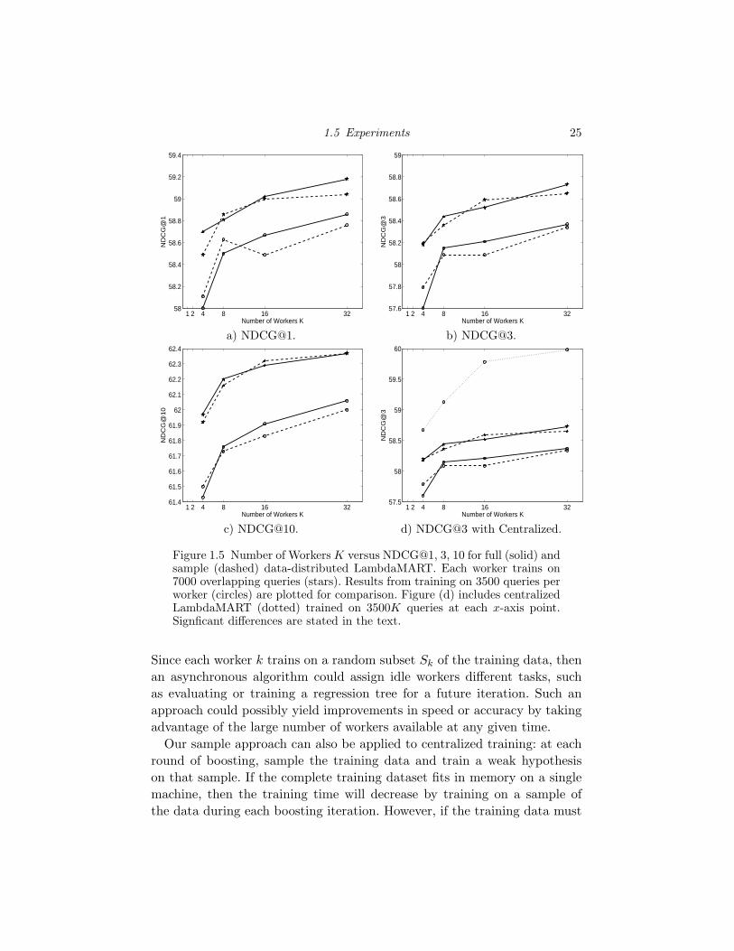
We first determine the effect of decreasing the training data size on the

centralized algorithm’s accuracy. Let the size of the training set residing on

the central machine decrease as |S|K

, with increasing values of K. Figure 1.6

plots the training set size versus NDCG for the centralized model (dotted

line). When training on 50% of the training data, the NDCG@1, 3, 10 accu-

racy compared to training on 100% of the data is statistically similar. It is

also noteworthy that as the training set size decreases, the optimal number

of leaves decreases, while the optimal learning rate stays constant across the

training data sizes (Table 1.1).

We next determine the accuracy of full and sample data-distributed Lamb-

daMART, where the training data S is split across K workers and each

worker contains |S|K

queries4. Figure 1.6 contains the centralized and full and

sample data-distributed accuracy results. In the central case, the x-axis indi-

cates the size of the training set on the single node. In the data-distributed

cases, the x-axis indicates the number of workers K and correspondingly

the amount of training data |S|K

on a given worker. The results indicate that

choosing a weak hypothesis among the K nodes, either by full or sample

selection, is better than choosing the same weak hypothesis from the same

node at each iteration. This is seen by looking at a given value of K: the

data-distributed NDCG scores are consistently higher than the centralized

4 The corresponding training time plot was given in Figure 1.3.

1.5 Experiments 27

1 2 4 8 16 3258

58.5

59

59.5

60

60.5N

DC

G@

1

Fraction of Training Data 1/K (Number of Workers K)1 2 4 8 16 32

57.5

58

58.5

59

59.5

60

ND

CG

@3

Fraction of Training Data 1/K (Number of Workers K)


1 2 4 8 16 3261

61.5

62

62.5

63

63.5

64

ND

CG

@10

Fraction of Training Data 1/K (Number of Workers K)

c) NDCG@10.

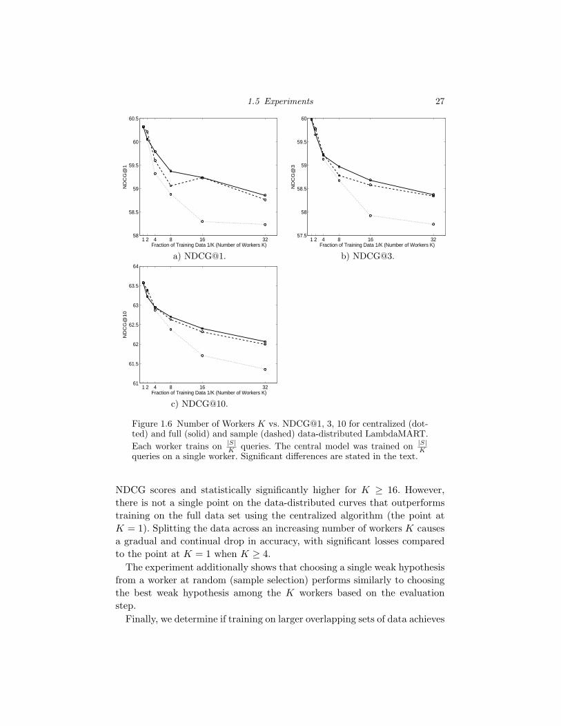
Figure 1.6 Number of Workers K vs. NDCG@1, 3, 10 for centralized (dot-ted) and full (solid) and sample (dashed) data-distributed LambdaMART.

Each worker trains on |S|K

queries. The central model was trained on |S|K

queries on a single worker. Significant differences are stated in the text.

NDCG scores and statistically significantly higher for K ≥ 16. However,

there is not a single point on the data-distributed curves that outperforms

training on the full data set using the centralized algorithm (the point at

K = 1). Splitting the data across an increasing number of workers K causes

a gradual and continual drop in accuracy, with significant losses compared

to the point at K = 1 when K ≥ 4.

The experiment additionally shows that choosing a single weak hypothesis

from a worker at random (sample selection) performs similarly to choosing

the best weak hypothesis among the K workers based on the evaluation

step.

Finally, we determine if training on larger overlapping sets of data achieves


comparable accuracy to the central model, but with less training time.

We consider K = 4 workers and divide the training data S into 4 sets

S1, S2, S3, S4. Each set contains 25% of the full training set. Worker k is

assigned sets Sk + Sk+1 + Sk+2, and thus produces a weak hypothesis based

on 75% of the full training set. At each iteration, we use sample selection to

produce the next weak hypothesis in the ensemble. We find that training on

75% of the training queries per node yields equivalent NDCG scores to the

central model trained on 100% of the training data, but trains in less than

half of the time.

Table 1.1 The learning rate η and the number of leaves L for centralized

LambdaMART, and full and sample data-distributed LambdaMART,

respectively. The first set of columns are the parameters when training on

3500 queries per worker; in the central case, a single worker trains on

3500K queries. The second set of columns are the parameters when

training on 7000 overlapping queries per worker; in the central case, a

single worker trains on 7000K queries. The final columns contain the

parameters when training on |S|K

queries per worker; in the central case, a

single worker trains on |S|K

queries.

3500 7000 All

K η L η L η L

1 0.1, 0.1, 0.1 20, 20, 20 0.1, 0.1, 0.1 80, 80, 80 0.1, 0.1, 0.1 20, 20, 20

2 0.1, 0.05, 0.05 80, 80, 80 0.1, 0.1, 0.1 180, 180, 180 0.1, 0.1, 0.1 80, 190, 200

4 0.1, 0.1, 0.05 180, 80, 80 0.1, 0.05, 0.05 200, 200, 200 0.1, 0.05, 0.05 180, 170, 200

8 0.1, 0.05, 0.05 200, 120, 120 0.1, 0.05, 0.05 200, 200, 200 0.05, 0.05, 0.05 200, 180, 200

16 0.1, 0.05, 0.05 200, 140, 140 0.1, 0.05, 0.05 200, 200, 200 0.1, 0.05, 0.05 200, 170, 160

32 0.1, 0.05, 0.05 200, 140, 140 0.1, 0.05, 0.05 200, 140, 140 0.1, 0.05, 0.05 200, 100, 140

1.6 Conclusions and Future Work

In summary, we have presented two approaches for distributing LambdaMART.

The first distributes by feature by distributing the vertex split computations

and requires that the full training set fit in main memory on each node in

the cluster. Our feature-distributed approach achieves up to 6-fold signif-

icant speed-ups over centralized LambdaMART while producing the same

model and accuracy. Our second approach distributes the data across the

nodes in the compute cluster and employs one of two strategies for selec-

1.7 Acknowledgements 29

tion of the next weak hypothesis: (1) select the next weak hypothesis based

on evaluation scores on the training data residing on other nodes (full) (2)

select the next weak hypothesis at random (sample). We have shown that

both selection strategies offer significant training time speed-ups resulting

in training up to 2–4 times faster than centralized LambdaMART. In par-

ticular, sample data-distributed LambdaMART demonstrates no significant

accuracy loss compared to full data-distributed LambdaMART, and achieves

even more significant training time speed-ups. Unlike the feature-distributed

approach, our data-distributed approaches can scale to billions of training

samples.

Our data-distributed algorithms, however, do not match the centralized

algorithm in accuracy. The accuracy results were disappointing and indicate

that using data for massive cross-validation results in significant accuracy

loss. In the future, it is worth determining a distributed method that can

scale to billions of examples, but with accuracy that is equivalent or superior

to training on centralized data, and with a communication cost that does not

scale with the number of samples. Future work needs to be done to determine

the bottlenecks of our data-distributed approaches, and to determine how

best to take advantage of distributed data without sacrificing the speed-ups

obtained by our methods. We have developed a first step toward achieving

this goal in that we have presented a method where the communication is

independent of the number of samples.

1.7 Acknowledgements

We thank Ofer Dekel for his insightful ideas, his invaluable contributions to

code and cluster development, and his assistance in running experiments.

References

Banko, M., and Brill, E. 2001. Scaling to Very Very Large Corpora for NaturalLanguage Disambiguation. Pages 26–33 of: Association for ComputationalLinguistics (ACL).

Burges, Christopher J., Svore, Krysta M., Benett, Paul N., Pastusiak, A., and Wu,Q. 2011. Learning to Rank Using an Ensemble of Lambda-Gradient Models.to appear in Special Edition of JMLR: Proceedings of the Yahoo! Learning toRank Challenge, 14, 25–35.

Burges, C.J.C. 2010. From RankNet to LambdaRank to LambdaMART: AnOverview. Tech. rept. MSR-TR-2010-82. Microsoft Research.

Burges, C.J.C., Ragno, R., and Le, Q.V. 2006. Learning to Rank with Non-Smooth Cost Functions. In: Advances in Neural Information Processing Sys-tems (NIPS).

Caragea, D., Silvescu, A., and Honavar, V. 2004. A framework for learning from dis-tributed data using sufficient statistics and it application to learning decisiontrees. International Journal of Hybrid Intelligent Systems, 1(1–2), 80–89.

Dean, J., and Ghemawat, S. 2004. MapReduce: Simplified data processing on largeclusters. In: Symposium on Operating System Design and Implementation(OSDI).

Domingos, P., and Hulten, G. 2000. Mining high-speed data streams. Pages 71–80of: SIGKDD Conference on Knowledge and Data Mining (KDD).

Domingos, P., and Hulten, G. 2001. A General Method for Scaling Up MachineLearning Algorithms and its Application to Clustering. In: International Con-ference on Machine Learning (ICML).

Donmez, P., Svore, K., and Burges, C.J.C. 2009. On the local optimality of Lamb-daRank. In: ACM SIGIR Conference on Research and Development in Infor-mation Retrieval (SIGIR).

Fan, W., Stolfo, S., and Zhang, J. 1999. The application of AdaBoost for dis-tributed, scalable and online learning. Pages 362–366 of: SIGKDD Conferenceon Knowledge and Data Mining (KDD).

Friedman, J. 2001. Greedy function approximation: a gradient boosting machine.Annals of Statistics, 25(5), 1189–1232.

Jarvelin, K., and Kekalainen, J. 2000. IR evaluation methods for retrieving highlyrelevant documents. Pages 41–48 of: ACM SIGIR Conference on Research andDevelopment in Information Retrieval (SIGIR).

References 33

Lazarevic, A. 2001. The distributed boosting algorithm. Pages 311–316 of: SIGKDDConference on Knowledge Discovery and Data Mining (KDD).

Lazarevic, A., and Obradovic, Z. 2002. Boosting Algorithms for Parallel and Dis-tributed Learning. Distributed and Parallel Databases, 11, 203–229.

Panda, B., Herbach, J. S., Basu, S., and Bayardo, R. J. 2009. PLANET: Mas-sively Parallel Learning of Tree Ensembles with MapReduce. In: InternationalConference on Very Large Databases (VLDB).

Provost, F., and Fayyad, U. 1999. A survey of methods for scaling up inductionalgorithms. Data Mining and Knowledge Discovery, 3, 131–169.

van Uyen, N. T., and Chung, T. 2007. A New Framework for Distributed BoostingAlgorithm. Pages 420–423 of: Future Generation Communication and Net-working (FGCN).

Wu, Q., Burges, C.J.C., Svore, K.M., and Gao, J. 2009. Adapting Boosting forInformation Retrieval Measures. Journal of Information Retrieval.

Yahoo! Learning to Rank Challenge. 2010. http://learningtorankchallenge.yahoo.com/.

Author index

λ-gradient, 7

boosted regression trees, 8, 9, 24data-distributed, 11, 14, 15feature-distributed, 10, 12

gradient boosted trees, 9, 24data-distributed, 11, 14, 15feature-distributed, 10, 12

lambda-gradient, 7LambdaMART, 7–9, 24

data-distributed, 11, 14, 15distributed, 10feature-distributed, 10, 12

LambdaRank, 7

MART, 8

NDCG, 7, 17Normalized Discounted Cumulative Gain, 7,

17

regression trees, 8

Subject index

λ-gradient, 7

boosted regression trees, 8, 9, 24data-distributed, 11, 14, 15feature-distributed, 10, 12

gradient boosted trees, 9, 24data-distributed, 11, 14, 15feature-distributed, 10, 12

lambda-gradient, 7LambdaMART, 7–9, 24

data-distributed, 11, 14, 15distributed, 10feature-distributed, 10, 12

LambdaRank, 7

MART, 8

NDCG, 7, 17Normalized Discounted Cumulative Gain, 7,

17

regression trees, 8

distributed machine learning - microsoft.com · machine learning algorithms into distributed...

Documents